15th meeting of the EURO Working Group on Transportation
Testing the validity of the MIP approach for locating carsharing stations in one-way systems
Diana Jorgea,*, Gonçalo Correiab, Cynthia Barnhartc aDepartment of Civil Engineering, University of Coimbra, Rua Luis Reis Santos, 3030-788 Coimbra, Portugal bDepartment of Civil Engineering, University of Coimbra, Rua Luis Reis Santos, 3030-788 Coimbra, Portugal
cDepartment of Civil and Environmental Engineering, Massachusetts Institute of Technology, 77 Massachusetts Avenue, Cambridge, MA,02139, USA
In the last decades there have been some changes in how the use of urban transportation is seen. Despite the advantages of the use of private transport, this has introduced serious negative externalities, such as pollution, and excessive consumption of energy and persons’ time due to congestion problems (Texas Transport Institute, 2010). Moreover, it presents very low utilization rates of each vehicle. A good alternative could be public transportation,
139 Diana Jorge et al. / Procedia - Social and Behavioral Sciences 54 ( 2012 ) 138 – 148
although it also has several problems, for instance, poor service coverage, and schedule inflexibility. So, there is now a general agreement on the need to find strategies that aim at minimizing these impacts and at the same time allowing persons to participate in the same activities as before. Carsharing is one of those strategies; it is a system that involves a small to medium fleet of vehicles available at several stations to be used by a relatively large group of members (Shaheen et al., 1999).
These systems have a positive impact on urban mobility mainly through a more efficient use of automobiles (Litman, 2000; Schuster et al., 2005). Shared vehicles can have much higher utilization rates than private vehicles. Typically the use of carsharing systems corresponds to a decrease on car ownership rates and as a consequence a reduction on car use as it was concluded by Celsor and Millard-Ball (2007). More recently, Schure et al. (2012) based on a survey conducted in 2010 in 13 buildings in downtown San Francisco concluded that the average vehicle ownership for households that use carsharing systems is 0.47 vehicles per household compared to 1.22 vehicles per household for households that do not use carsharing systems. This illustrates the potential of carsharing systems as a strong transport demand management measure.
The origins of shared-use vehicles can be traced back to 1948 in Europe (Shaheen et al., 1999). In the United States, these systems appeared much later, in 1983, within the Mobility Enterprise program. US first adopters were motivated more by convenience than by affordability, possibly due to the lower costs of driving in the US (Lane, 2005).
Carsharing systems can be classified with respect to several parameters (Correia and Antunes, 2012), being the most common the trip configuration, which includes one-way systems and round-trip (or two-way) systems (Shaheen et al., 2006). Traditional carsharing systems operators require users to return cars to the same station where they were picked up. These are round-trip carsharing systems, which simplify the task of the operators because they may plan stocks based on the demand for each station, however this is often inconvenient for the users. More convenient systems for the users are one-way carsharing systems. In this kind of systems, users can pick up a car in one station and return it to a different one. Thus, in theory, one-way carsharing systems allow capturing a higher number of trips when compared to the round-trip alternative which can only be used by a small share of the market, such as leisure, shopping and sporadic trips (Barth and Shaheen, 2002). However, since demand for vehicles and parking spaces fluctuates, there is always a tendency for the system to become unbalanced. This is probably the main reason why there have been very few attempts to provide one-way carsharing systems. One example was in Singapore, but with poor success (Mitchell et al., 2010), since as the membership grew, the operator could not keep up the initial service quality, so dissatisfaction and complaints from members increased (The Straits Times, 2008), which caused the end of the service.
Several approaches have been proposed to solve the imbalance problem. Kek et al. (2006) and Kek et al. (2009) proposed the operator-based approach that corresponds to the periodic relocation of vehicles among stations by staff members. Fan et al. (2008) studied the trip allocation approach, where the manager has full operational control of which trips to accept or refuse in order to achieve a more favorable balance of vehicle stocks. Correia and Antunes (2012) developed the station location approach, which corresponds to plan the carsharing stations’ location to try capturing a better trip pattern that leads to a more convenient distribution of vehicles in the network and studied it simultaneously with the trip allocation approach. The techniques that were predominantly used were simulation and mathematical programming. Despite the positive results of demonstrating that there are operating principles that can improve these systems’ viability, these modeling tools have limitations: while simulation implies an impractical number of runs to test all the combinations of the different operational parameters (Kek et al., 2006), optimization implies a large number of variables to integrate several decisions in the same problem in a real case study context (Correia and Antunes, 2012), which implies the simplification of the formulations to a level where they may be unrealistic and the efficiency improvements extracted from them may be hard to transfer to real carsharing systems. Moreover, even with these simplifications many times is not possible to include several decisions in the same formulation. Taking into consideration these findings, in this paper we decided to build an agent-based simulation model based on the mixed-integer programming (MIP) model developed by Correia and Antunes (2012) for the
140 Diana Jorge et al. / Procedia - Social and Behavioral Sciences 54 ( 2012 ) 138 – 148
problem of choosing carsharing stations location when all the trips between existing stations must be accepted, and test the solutions obtained by them in the hypothesis of having relocation operations between stations. In addition, mathematical programming models have difficulties including uncertainty, thus, we also test different scenarios regarding the demand pattern in order to assess its impact on the solutions.
The structure of the paper is the following. In the next section we present the MIP model developed by Correia and Antunes (2012). Afterward, the agent-based simulation model is presented. The Lisbon case study is presented in the fourth section. This is followed by the results of testing trip variability and relocation operations. The paper finishes with the main conclusions obtained in this work.
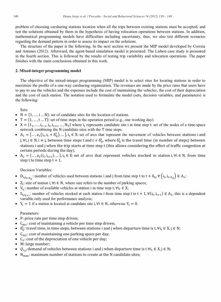
2. Mixed-integer programming model
The objective of the mixed-integer programming (MIP) model is to select sites for locating stations in order to maximize the profits of a one-way carsharing organization. The revenues are made by the price rates that users have to pay to use the vehicles and the expenses include the cost of maintaining the vehicles, the cost of their depreciation and the cost of each station. The notation used to formulate the model (sets, decision variables, and parameters) is the following:
Sets: set of candidate sites for the location of stations. set of time steps in the operation period (e.g., one working day). where represents candidate site at time step set of the nodes of a time-space
network combining the candidate sites with the time steps. set of arcs that represent the movement of vehicles between
Decision Variables:
number of vehicles used between stations and from time step to ;
size of station , where size refers to the number of parking spaces; number of available vehicles at station in time step ; : number of vehicles stocked at each station from time step to , this is a dependent
variable only used for performance analysis; if a station is located at candidate site , otherwise .
Parameters:
141 Diana Jorge et al. / Procedia - Social and Behavioral Sciences 54 ( 2012 ) 138 – 148
Using the notation above, the MIP model can be formulated as follows:
(1)
subject to,
(2)
(3)
(4)
(5)
(6)
(7)
(8)
(9)
(10)
(11)
(12)
(13)
(14)
(15)
The objective function (1) of the MIP model maximizes the total daily profit of the one-way carsharing
organization, taking into consideration the revenues obtained through the trips paid by clients, the vehicle
142 Diana Jorge et al. / Procedia - Social and Behavioral Sciences 54 ( 2012 ) 138 – 148
maintenance costs, the stations maintenance costs, and the vehicle depreciation costs. Constraints (2) ensure the conservation of vehicle flows at each node of the time-space network and update the number of vehicles available at each station at time step taking into consideration the number of vehicles at time step . Constraints (3) compute the vehicle stocks available at each station from to . Constraints (4) guarantee that the size of the station of site is greater than the number of vehicles present there at each time step . In practice, size will not be greater than the highest value of for the operation period because this would penalize the objective function. Constraints (5) prevent vehicles to be stocked at sites where there are no stations and constraints (6) specify that the size of any station is at least one parking space. Constraints (7) ensure that the number of performed trips between stations and at time step will not exceed demand. Constraint (8) is optional and it defines the maximum number of stations (if then it is possible to locate a station in each candidate site). Constraint (9) is also optional and it guarantees that the satisfied demand is above the minimum limit . Constraints (10) ensure that all the demand between existing stations is satisfied, since constraints (7) obligate . All the demand between existing stations has to be satisfied does not mean to have all locations with a station, it is possible to have a lower number of stations, where all the specific trips between those stations are performed. Only if , all the trips in the model have to be satisfied, in that case all stations must be located and the decision is immediate. The difference is: all the demand in the city or all the demand specific to the existing stations. Expressions (11)-(15) set the domain for the decision variables.
3. Agent-based simulation model
Agent-based simulation models contain agents who interact between them within a given environment. Besides the interactions agent-agent, there are other type of interactions, namely agent-environment and environment-environment. Each agent has the possibility of choosing one or more actions from a set of possible actions and has an internal state that contains information from the past. He will act according to this and some rules of behavior. On the one hand, these actions will produce consequences in the environment, and on the other hand, the environment influences the rules of behavior of the agents.
In the case of our agent-based simulation model, agents are the travelers and the environment is the case study city. This is a very simple model, since it has to reproduce exactly what happens in the MIP model. The model was built using AnyLgoc (xj technology) and has as its main experimental factor the location of carsharing stations. Each trip will only be performed if there are simultaneously the station where it starts and the station where it ends. The road network (environment) influences the system through congestion levels affecting travel time, since we considered different times of the day: morning peak, the afternoon peak, and the rest of the day.
In each time step (a time step of 10 minutes was used in the MIP model), the trips are triggered and the model updates: the number of completed time steps driven, the vehicles’ availability in each station, the total vehicle fleet needed, and the maximum stocks of vehicles in each station (the maximum number of vehicles that were parked for all the time steps until the current one) which is used to compute the stations dimension. Considering that in this model, all the demand between the existing stations must be satisfied, each time a vehicle is needed in a given station for a given trip and there are no vehicles available in that station, the model creates a vehicle, increasing the fleet. In the end of the simulation, period between 6 a.m. and mid-night, the model computes several indicators, namely the total profit, the total number of parking spaces, the vehicle use, the profit per vehicle, the profit per station, the percentage of demand satisfied, and the number of vehicles per 100 trips.
3.1. Demand variability
To introduce demand variability in the model, we consider that each of the trips used as input in the MIP model (Correia and Antunes, 2012) has a probability of being performed. This probability corresponds to a parameter, which can be varied in order to test different scenarios. The process works as following: through the Monte Carlo
143 Diana Jorge et al. / Procedia - Social and Behavioral Sciences 54 ( 2012 ) 138 – 148
method, a random number is generated and associated to each trip, if this number is smaller than the probability, the trip is performed, otherwise the trip is not performed.
3.2. Relocation policy
We develop a simple relocation policy where for each time step and station we decide whether that station can offer vehicles to other stations (supply) or that station needs vehicles (demand) taking into consideration what happens two time steps after in terms of historical balance of trips (Entries-Exits). If that number is positive, that station is a potential supplier of vehicles and the potential maximum supply is equal to the availability in the current time step (number of vehicles that are available in that station after the exits in the current time step). If that number is negative, that station has a need for vehicles, which is equal to that number. When the station is in equilibrium, this number is equal to zero. This means that a station can only be in one of these states in each time step. In this relocation policy, there are two possible parameters to vary: one is the relocation percentage, which is the percentage of current vehicle availability of each supplier station that can be relocated to the stations that need vehicles; and the other is the frequency with which the relocations are triggered (every time step, every two time steps, etc).
To decide how many vehicles should be relocated between existing stations, we solve a typical transportation problem in Operational Research where we must meet the demand with the available supply with a minimum cost. This is usually solved by the stepping stone or multipliers methods however we solve it using the minimum cost flow algorithm in a network because this algorithm was already programmed in Java (Anylogic works on Java) (Lau, 2007). In the network we have the supply nodes (stations that can offer vehicles), the demand nodes (stations that need vehicles), and an artificial supply node as well as an artificial demand node, where all total supply and demand are concentrated. The artificial supply node is connected to the supply nodes, these are linked to the demand nodes, and finally the demand nodes are linked to the artificial demand node. This is shown in Fig. 1. For each arc we define three different parameters: the cost of the arc (travel time), the lower bound (minimum number of vehicles), and the upper bound (maximum number of vehicles). In the arcs between the artificial supply node and the supply nodes the lower and upper bounds are equal and correspond to the supply in each supply node. For the arcs between supply nodes and demand nodes, the lower bound is zero and the upper bound is the minimum of the number of vehicles that the supply node can offer and the number of vehicles that the demand node can receive. In the arcs between the demand nodes and the artificial demand node, the lower and upper bounds are the same, corresponding to the demand in each demand node.
Fig. 1. Minimum cost flow algorithm scheme
After the optimization model is run the time needed to relocate the vehicles between supply and demand stations
is summed to the objective function as an extra cost of 2€ per time step (equation (1)).
144 Diana Jorge et al. / Procedia - Social and Behavioral Sciences 54 ( 2012 ) 138 – 148
4. Lisbon case study
The case study is the municipality of Lisbon, the capital city of Portugal, the same that was used in the optimization approach (Correia and Antunes, 2012). The types of data that are needed to apply the model are: the potential trip matrix, the candidate station locations, the driving travel times, and the costs of running the system. The trip matrix was obtained through a survey which was filtered in order to consider only the trips that can be captured by this system, resulting in 1776 trips. The candidate station locations were defined by considering a grid of squared cells with 1000m side over Lisbon and associating one location with the center of each cell resulting in a total of 75 station locations (Fig. 2). Travel times were computed using the transportation modeling software VISUM (PTV), and were expressed in time steps of 10 minutes. Since the carsharing system is available18 hours per day (between 6:00 a.m. and 12:00 p.m.), 108 time steps were considered. The costs of running the system were:
(cost of maintaining a vehicle): 0.07 euros per 10 min; (cost of relocating a vehicle): 2 euros per 10 min, since the average hourly wage in Portugal is 12 euros per
hour; (cost of maintaining a parking space): 5 euros per day, the parking fee in a low price area in London; (cost of the depreciation of one vehicle): 17 euros per day, calculated for a city car.
The price rate, , was considered to be 4 euros per 10 min. Correia and Antunes (2012) chose this value, which is
unrealistic comparing for example with the price rates of Car2Go (Car2Go, 2011), a one-way carsharing company that operates in Europe, since with lower values it was not possible to find a solution with a positive profit that satisfied all trips between stations.
Fig. 2. Simulation visualization of the municipality of Lisbon with the 75 possible stations location
145 Diana Jorge et al. / Procedia - Social and Behavioral Sciences 54 ( 2012 ) 138 – 148
5. Results
In the MIP approach by Correia and Antunes (2012), three different scenarios were considered: the first scenario, with all stations located (75 stations); the second scenario, which is the optimum scenario, with 34 stations located; and a third scenario, limiting the maximum number of stations to 10.
5.1. Demand variability results
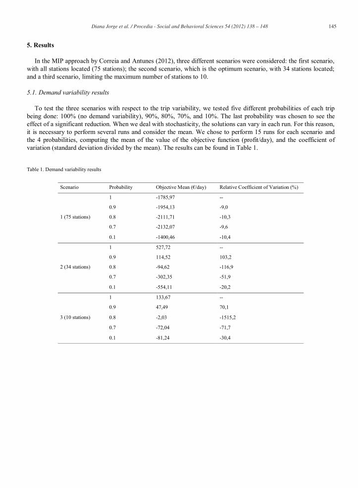
To test the three scenarios with respect to the trip variability, we tested five different probabilities of each trip being done: 100% (no demand variability), 90%, 80%, 70%, and 10%. The last probability was chosen to see the effect of a significant reduction. When we deal with stochasticity, the solutions can vary in each run. For this reason, it is necessary to perform several runs and consider the mean. We chose to perform 15 runs for each scenario and the 4 probabilities, computing the mean of the value of the objective function (profit/day), and the coefficient of variation (standard deviation divided by the mean). The results can be found in Table 1.
Table 1. Demand variability results
Scenario Probability Objective Mean (€/day) Relative Coefficient of Variation (%)
1 (75 stations)
1 -1785,97 --
0.9 -1954,13 -9,0
0.8 -2111,71 -10,3
0.7 -2132,07 -9,6
0.1 -1400,46 -10,4
2 (34 stations)
1 527,72 --
0.9 114,52 103,2
0.8 -94,62 -116,9
0.7 -302,35 -51,9
0.1 -554,11 -20,2
3 (10 stations)
1 133,67 --
0.9 47,49 70,1
0.8 -2,03 -1515,2
0.7 -72,04 -71,7
0.1 -81,24 -30,4
146 Diana Jorge et al. / Procedia - Social and Behavioral Sciences 54 ( 2012 ) 138 – 148
As we can see in Table 1, for scenario 1, as we decrease the probability, the mean value of the objective function will also decrease, until we decrease the demand to a level where some stations disappear, since they have no parking spaces. This can be seen with the 10% probability. The relative coefficients of variation are about 10%, which means that the deviations with respect to the mean reach about 10% of its value. For scenarios 2 and 3, as we decrease the probability, the mean value of the objective function will also decrease for all the probabilities, since decreasing the trips is not enough to decrease the number of vehicles and parking spaces that are necessary for profit maximization. The relative coefficients of variation vary between 20.2% and 1515.2%, which is a high value. These results show that demand variability has a significant impact on the profit. Therefore, using a deterministic demand to optimize the location of the stations as happens in the MIP approach is a limitation because trips are never the same.
5.2. Relocation operations results
Considering all the demand between existing stations, for each scenario we introduce the relocations firstly by changing only the relocation percentage between 0% (no relocations) and 100% (all available vehicles in supply stations can be relocated), and in 10% increments. The relocations are triggered every time step. The results related to the number of vehicles, the number of parking spaces and the value of the objective function (profit) are shown in Table 2.
For scenario 1 (75 stations located), it is possible to decrease the losses introducing this relocation policy for all
the relocation percentages, except for the 100%. The best relocation percentage is 50%, which allows a reduction in losses from -1785.97€/day to -76.97€/day. This is achieved because due to relocations the number of vehicles and the number of parking spaces needed has decreased significantly.
With respect to scenarios 2 (optimum) and 3 (optimum with 10 stations limitation), the introduction of the relocation policy does not allow increasing the profit for any of the percentages considered. The best profit is
147 Diana Jorge et al. / Procedia - Social and Behavioral Sciences 54 ( 2012 ) 138 – 148
obtained when no vehicles are relocated. This may happen because the stations’ location was tailored to the demand in these two scenarios; it is already very efficient when compared to the 75 stations scenario that covers the entire city and has to satisfy all demand.
Considering the best relocation percentages for each scenario: 50%, 10%, and 50%, respectively, we varied the frequency with which the relocations are triggered between 20 and 60 minutes in increments of 10 minutes. Analyzing the results, we verified that only for scenario 2 it is possible to increase the profit. With a relocation frequency of 40 minutes, the profit has a slight increase above the reference obtained with no relocations, from 527.72€/day to 554.52€/day.
5.3. Demand variability and relocation operations results
We also want to see what happens if we introduce simultaneously demand variability and the relocation policy, so for each scenario and probability with respect to the demand variability, excluding 100%, we varied the relocation percentage between 10% and 100% in 10% steps. We concluded that when demand variability and relocation operations are simultaneously introduced, there are improvements in the profit for some relocation percentages even for scenarios 2 and 3 related to the solution with no relocations, which does not happen with relocations operations only, since the stations’ location was tailored to all the demand in these two scenarios.
6. Conclusions
The most convenient carsharing systems for users are the one-way systems; however they present some management problems to the operators. Several approaches have been proposed to try solving these problems, such as the operator-based approach (Kek et al., 2009) and the station location approach (Correia and Antunes, 2012) which use optimization as their main modeling tool. In this article we have picked up the model by Correia and Antunes (2012) and have used simulation in order to introduce demand variability and test the effect that vehicle relocations may have in the deterministic solutions obtained by these authors. We were able to conclude that both demand variability and the relocation operations have a significant impact on the solutions. With respect to demand variability we concluded that in general the reduction in the demand has a negative impact on the solutions, decreasing the profit, even if it is possible to save money on vehicles and parking spaces. The opposite only occurs when the demand is decreased to a level in which some stations disappear. This happens for the scenario where all possible locations have stations and with a probability of only 10% of each sampled trip being performed. Introducing the relocation policy with no demand variability, we conclude that it allows significant reductions in the losses when 75 stations are located (the whole city covered), but does not allow improving the profit for 34 and 10 stations located which have been tailored to maximize the profit confirming the influence of the stations’ location in the operation of these systems. According to the results, the main conclusion that we can withdraw from this work is that demand variability should be included in the planning models for one-way carsharing and that several operational options, such as relocation operations, should be studied in an integrated way, since both of these factors cause significant impacts on the solutions. The next step will be comparing the results obtained through simulation for this relocation policy with the optimum relocations in order to propose the best policies.
Acknowledgements
The research in which this article is based was carried out within the framework of a PhD thesis of the MIT Portugal Program. The authors wish to thank Fundação para a Ciência e a Tecnologia for financing this PhD project through a scholarship.
148 Diana Jorge et al. / Procedia - Social and Behavioral Sciences 54 ( 2012 ) 138 – 148
References
Barth, M., & Shaheen, S. (2002). Shared-Use Vehicle Systems: Framework for Classifying Carsharing, Station Cars, and Combined Approaches. Transportation Research Record: Journal of the Transportation Research Board, 1791, 105-112. Car2Go (2011). <http://www.car2go.com/> (accessed 04.07.11). Celsor, C., & Millard-Ball, A. (2007). Where Does Carsharing Work?: Using Geographic Information Systems to Assess Market Potential. Transportation Research Record: Journal of the Transportation Research Board, 1992, 61-69. Correia, G., & Antunes, A.P. (2012). Optimization approach to depot location and trip selection in one-way carsharing systems. Transportation Research Part E: Logistics and Transportation Review, 48, 233-247. Fan, W., Machemehl, R., & Lownes, N. (2008). Carsharing: Dynamic Decision-Making Problem for Vehicle Allocation. Transportation Research Record: Journal of the Transportation Research Board, 2063, 97-104. Kek, A., Cheu, R., & Chor, M. (2006). Relocation Simulation Model for Multiple-Station Shared-Use Vehicle Systems. Transportation Research Record: Journal of the Transportation Research Board, 1986, 81-88. Kek, A., Cheu, R., Meng, Q., & Fung, C. (2009). A decision support system for vehicle relocation operations in carsharing systems. Transportation Research Part E: Logistics and Transportation Review, 45, 149-158. Lane, C. (2005). PhillyCarShare - First-year social and mobility impacts of carsharing in Philadelphia, Pennsylvania. Transportation Research Record: Journal of the Transportation Research Board, 1927, 158-166. Lau, H. (2007). A Java Library of Graph Algorithms and Optimization. Chapman & Hall/CRC, (Chapter 8). Litman, T. (2000). Evaluating Carsharing Benefits. Transportation Research Record: Journal of the Transportation Research Board, 1702, 31-35. Mitchell, W., Borroni-Bird, C., & Burns, L. (2010). Reinventing the Automobile: personal urban mobility for the 21st century. Cambridge, Massachusetts: MIT Press, (Chapter 8). Schure, J.t., Napolitan, F., Hutchinson, R. (2012) Cumulative Impacts of Carsharing and Unbundled Parking on Vehicle Ownership & Mode Choice. In: 91st Annual Meeting of Transportation Research Board, Washington DC, USA, January 22-26, 2012. Schuster, T.D., Byrne, J., Corbett, J., & Schreuder, Y. (2005). Assessing the potential extent of carsharing - A new method and its applications. Transportation Research Record: Journal of the Transportation Research Board, 1927, 174-181. Shaheen, S., Cohen, A., & Roberts, J. (2006). Carsharing in North America: Market Growth, Current Developments, and Future Potential. Transportation Research Record: Journal of the Transportation Research Board, 1986, 116-124. Shaheen, S., Sperling, D., & Wagner, C. (1999). A Short History of Carsharing in the 90's. Journal of World Transport Policy and Practice, 5, 16-37. Texas Transport Institute (2010). The 2010 Urban Mobility Report. The Straits Times (2008) End of the Road for Honda Car Sharing Scheme. 29 February, 2008