Testing theoryP.J.G. Teunissen

Series on Mathematical Geodesy and Positioning

an introduction

Testing theoryan introduction

Testing theoryan introduction

P.J.G. Teunissen

Delft University of Technology

Department of Mathematical Geodesy and Positioning

VSSD

Series on Mathematical Geodesy and Positioninghttp://www.vssd.nl/hlf/a030.htm

Adjustment TheoryP.J.G. Teunissen2003 / 201 p. / ISBN 90-407-1974-8

Dynamic Data ProcessingP.J.G. Teunissen2001 / 241 + x p. / ISBN 90-407-1976-4

Testing TheoryP.J.G. Teunissen2000 / 147+viii p. / ISBN 90-407-1975-6

HydrographyC.D. de Jong, G. Lachapelle, S. Skone, I.A. Elema2003 / x+351 pp. / ISBN 90-407-2359-1 / hardback

© VSSD

First edition 2000-2006

Published by:VSSDLeeghwaterstraat 42, 2628 CA Delft, The Netherlandstel. +31 15 278 2124, telefax +31 15 278 7585, e-mail: hlf@vssd.nlinternet: http://www.vssd.nl/hlfURL about this book: http://www.vssd.nl/hlf/a030.htm

A collection of digital pictures and an elctronic version can be made availablefor lecturers who adopt this book. Please send a request by e-mail tohlf@vssd.nl

All rights reserved. No part of this publication may be reproduced, stored in aretrieval system, or transmitted, in any form or by any means, electronic,mechanical, photocopying, recording, or otherwise, without the prior writtenpermission of the publisher.

Printed version: ISBN 978-90-407-1975-2 Ebook: ISBN 978-90-6562-216-7NUR 930

Keywords: testing theory, geodesy

Foreword

This book is based on the lecture notes of the course ’Testing theory’ (Inleiding Toetsingstheorie)as it has been offered since 1989 by the Department of Mathematical Geodesy and Positioning(MGP) of the Delft University of Technology. This course is a standard requirement and is givenin the second year. The prerequisites are a solid knowledge of adjustment theory together withlinear algebra, statistics and calculus at the undergraduate level. The theory and application ofleast-squares adjustments are treated in the lecture notes Adjustment theory (Delft UniversityPress, 2000). The material of the present course is a follow up on this course on adjustmenttheory. Its main goal is to convey the knowledge necessary to be able to judge and validate theoutcome of an adjustment. As in other physical sciences, measurements and models are used inGeodesy to describe (parts of) physical reality. It may happen however, that some of themeasurements or some parts of the model are biased or in error. The measurements, for instance,may be corrupted by blunders, or the chosen model may fail to give an adequate enoughdescription of physical reality. These mistakes can and will occasionally happen, despite the factthat every geodesist will try his or her best to avoid making such mistakes. It is therefore ofimportance to have ways of detecting and identifying such mistakes. It is the material of thepresent lecture notes that provides the necessary statistical theory and testing procedures forresolving situations like these.

Following the Introduction, the basic concepts of statistical testing are presented in Chapter 1.In Chapter 2 the necessary theory is developed for testing simple hypotheses. As opposed to itscomposite counterpart, a simple hypothesis is one which is completely specified, both in itsfunctional form as well as in the values of its parameters. Although simple hypotheses rarelyoccur in geodetic practice, the material of this chapter serves as an introduction to the chaptersfollowing. In Chapter 3, the generalized likelihood ratio principle is used to develop the theoryfor testing composite hypotheses. This theory is then worked out in detail in Chapter 4, for theimportant case of linear(ized) models. Both the parametric form (observation equations) and theimplicit form (condition equations) of linear models are treated. Five different expressions aregiven for the uniformly, most powerful, invariant teststatistic. As an additional aid inunderstanding the basic principles involved, a geometric interpretation is given throughout. Thischapter also introduces the important concept of reliability. The internal and external reliabilitymeasures given, enable a user to determine in advance (i.e. at the designing stage, before theactual measurements are collected) the size of the minimal detectable biases and the size of theirpotential impact on the estimated parameters of interest.

Many colleagues of the Department of Mathematical Geodesy and Positioning whose assistancemade the completion of this book possible are greatly acknowledged. C.C.J.M. Tiberius took careof the editing, while the typing was done by Mrs. J. van der Bijl and Mrs. M.P.M. Scholtes. Thedrawings were made by Mr. A.B Smits and the statistical tables were generated by Mrs. M.Roselaar. Various lecturers have taught the book’s material over the past years. In particular thefeedback and valuable recommendations of G.J. Husti, F. Kenselaar and N.F. Jonkman areacknowledged.

P.J.G. TeunissenJune, 2000

Contents

Introduction . . . . . . . . . . . . . . . . . . . . . . . . . . . . . . . . . . . . . . . . . . . . . . . . . . . . . . . 1

1 Basic concepts of hypothesis testing . . . . . . . . . . . . . . . . . . . . . . . . . . . . . . . . . 5

1.1 Statistical hypotheses . . . . . . . . . . . . . . . . . . . . . . . . . . . . . . . . . . . . . 51.2 Test of statistical hypotheses . . . . . . . . . . . . . . . . . . . . . . . . . . . . . . . . 81.3 Two types of errors . . . . . . . . . . . . . . . . . . . . . . . . . . . . . . . . . . . . . 101.4 A testing principle . . . . . . . . . . . . . . . . . . . . . . . . . . . . . . . . . . . . . . 161.5 General steps in testing hypotheses . . . . . . . . . . . . . . . . . . . . . . . . . . . 19

2 Testing of simple hypotheses . . . . . . . . . . . . . . . . . . . . . . . . . . . . . . . . . . . . . 21

2.1 The simple likelihood ratio test . . . . . . . . . . . . . . . . . . . . . . . . . . . . . 212.2 Most powerful tests . . . . . . . . . . . . . . . . . . . . . . . . . . . . . . . . . . . . . 292.3 The -teststatistic . . . . . . . . . . . . . . . . . . . . . . . . . . . . . . . . . . . . . . 35w2.4 The -teststatistic . . . . . . . . . . . . . . . . . . . . . . . . . . . . . . . . . . . . . . . 48v

3 Testing of composite hypotheses . . . . . . . . . . . . . . . . . . . . . . . . . . . . . . . . . . . 53

3.1 The generalized likelihood ratio test . . . . . . . . . . . . . . . . . . . . . . . . . . 533.2 Uniformly most powerful tests . . . . . . . . . . . . . . . . . . . . . . . . . . . . . 62

4 Hypothesis testing in linear models . . . . . . . . . . . . . . . . . . . . . . . . . . . . . . . . . 71

4.1 The models of condition and observation equations . . . . . . . . . . . . . . . 714.2 A geometric interpretation of . . . . . . . . . . . . . . . . . . . . . . . . . . . . 79T

q4.3 The case q = 1: the -teststatistic . . . . . . . . . . . . . . . . . . . . . . . . . . . 86w4.4 The case q = m−n: the -teststatistic . . . . . . . . . . . . . . . . . . . . . . . . . 90σ̂2

4.5 Internal reliability . . . . . . . . . . . . . . . . . . . . . . . . . . . . . . . . . . . . . . . 944.6 External reliability . . . . . . . . . . . . . . . . . . . . . . . . . . . . . . . . . . . . . 1104.7 Reliability: an example . . . . . . . . . . . . . . . . . . . . . . . . . . . . . . . . . . 118

Appendices . . . . . . . . . . . . . . . . . . . . . . . . . . . . . . . . . . . . . . . . . . . . . . . . . . . . . . 124

A Some standard distributions . . . . . . . . . . . . . . . . . . . . . . . . . . . . . . . 124B Statistical tables . . . . . . . . . . . . . . . . . . . . . . . . . . . . . . . . . . . . . . . 126C Detection, identification and adaptation . . . . . . . . . . . . . . . . . . . . . . . 132D Early history of adjusting geodetic and astronomical observations . . . . 137

Literature . . . . . . . . . . . . . . . . . . . . . . . . . . . . . . . . . . . . . . . . . . . . . . . . . . . . . . . 145Index . . . . . . . . . . . . . . . . . . . . . . . . . . . . . . . . . . . . . . . . . . . . . . . . . . . . . . . . . . 147

Introduction

The present lecture notes are a follow up on the book Adjustment theory (Delft University Press,2000). Adjustment theory deals with the optimal combination of redundant measurementstogether with the estimation of unknown parameters. There are two main reasons for performingredundant measurements. First, the wish to increase the accuracy of the results computed.Second, the requirement to be able to check for mistakes or errors. The present book addressesthis second topic.

In order to be able to adjust redundant observations, one first needs to choose a mathematicalmodel. This model consists of two parts, the functional model and the stochastic model. Thefunctional model contains the set of functional relations the observables are assumed to obey.For instance, when the three angles of a triangle are observed and when it is assumed that thelaws of planar Euclidean geometry apply, the three angles should add up to π. However, sincemeasurements are intrinsically uncertain (perfect measurements do not exist), one should alsotake the unavoidable variability of the measurements into account. This is done by means of astochastic model in which the measurement uncertainty is captured through the use of stochastic(or random) variables. In most geodetic applications it is assumed that the results ofmeasurement, the observations, are independent samples drawn from a normal (or Gaussian)distribution.

Once the mathematical model is specified, one can proceed with the adjustment. Althoughdifferent methods of adjustment exist, one of the leading principles is the principle ofleast-squares (for a brief account on the early history of adjustment, see Appendix D). Apartfrom the fact that (linear) least-squares estimators are relatively easy to compute, they alsopossess two important properties, namely the property of unbiasedness and the property ofminimum variance. In layman terms one could say that least-squares solutions coincide with theirtarget value on the average (property of unbiasedness), while the sum of squares of theirunavoidable, individual variations about this target value will be the smallest possible on theaverage (property of minimum variance). These two properties only hold true, however, underthe assumption that the mathematical model is correct. They fail to hold in case the mathematicalmodel is misspecified. Errors or misspecifications in the functional model generally result inleast-squares estimators that are biased (off target). Similarly, misspecifications in the stochasticmodel will generally result in least-squares estimators that are less precise (larger variations).

Although one always will try one’s best to avoid making mistakes, they can and will occasionallyhappen. It is therefore of importance to have ways of detecting and identifying such mistakes.In this book we will restrict ourselves and concentrate only on developing methods for detectingand identifying errors in the functional model. Hence, throughout this book the stochastic modelis assumed to be specified correctly. This restriction is a legitimate one for many geodeticapplications. From past experience we know that if modelling errors occur, they usually occurin the functional model and not so much in the stochastic model. Putting the exceptions aside,one is usually quite capable of making a justifiable choice for the stochastic model. Moreover,mistakes made in the functional model usually have more serious consequences for the resultscomputed than errors made in the stochastic modelling.

2 Testing theory

Mistakes or errors in the functional model can come in many different guises. At this point itis of importance to realize, since every model is a caricature of reality, that every model has itsshortcomings. Hence, strictly speaking, every model is already in error to begin with. This showsthat the notion of a modelling error or a model misspecification has to be considered with somecare. In order to understand this notion, it helps if one accepts that the presence of modellingerrors can only be felt in the confrontation between data and model. We therefore speak of amodelling error when the discrepancies between the observations and the model are such thatthey can not be explained by, or attributed to, the unavoidable measurement uncertainty. Suchdiscrepancies can have many different causes. They could be caused by mistakes made by theobserver, or by the fact that defective instruments are used, or by wrong assumptions about thefunctional relations between the observables. For instance, in case of levelling, it could happenthat the observer made a mistake when reading off the leveling rod, or in case of directionmeasurements, it could happen that the observer accidentally aimed the theodolite at the wrongpoint. These types of mistakes affect individual observations and are usually referred to asblunders or gross errors. Instead of a few individual observations, whole sets of observations maybecome affected by errors as well. This happens in case defective instruments are used, or whenmistakes are made in formulating the functional relations between the observables. Errors witha common cause that affect whole sets of observations are sometimes referred to as systematicerrors.

The goal of this book is to convey the necessary knowledge for judging the validity of the modelused. Typical questions that will be addressed are: ’How to check the validity of a model? Howto search for certain mistakes or errors? How well can errors be traced? How do undetectederrors affect the final results?’ As to the detection and identification of errors, the general stepsinvolved are as follows:(i) One starts with a model which is believed to give an adequate enough description of

reality. It is usually the simplest model possible which on the basis of past experience hasproven itself in similar situations. Since one will ordinarily assume that the measurementsand the modelling are done with the utmost care, one is generally not willing, at thisstage, to already make allowances for possible mistakes or errors. This is of course anassumption or an hypothesis. This first model is therefore referred to as the nullhypothesis.

(ii) Since one can never be sure about the absence of mistakes or errors, it is always wise tocheck the validity of the null hypothesis once it has been selected. Hence, one would liketo be able to detect an untrustworthy null hypothesis. This is possible in principle, whenredundant measurements are available. From the adjustment of the redundantmeasurements, (least-squares) residuals can be computed. These residuals are a measureof how well the measurements fit the model of the null hypothesis. Large residuals areoften indicative for a poor fit, while smaller residuals tend to correspond with a better fit.These residuals are therefore used as input for deciding whether or not one is willing toaccept the null hypothesis.

(iii) Would one decide to reject the null hypothesis, one implicitly states that themeasurements do not seem to support the assumption that the model under the nullhypothesis gives an adequate enough description of reality. One will therefore have tolook for an alternative model or an alternative hypothesis. It very seldom happens

Introduction 3

however, that one knows beforehand which alternative to consider. After all, manydifferent errors could have led to the rejection of the null hypothesis. This implies thatin practice, instead of considering a single alternative, usually various alternatives willhave to be considered. And since different types of errors may occur in differentsituations, the choice of these alternatives very much depends on the particular situationat hand.

(iv) Once it has been decided which alternatives to consider, one can commence with theprocess of identifying the most likely alternative. This in fact boils down to a search ofthe alternative hypothesis which best fits the measurements. Since each alternativehypothesis describes a particular mistake or modelling error, the most likely mistakecorresponds with the most likely hypothesis. Once one is confident that the modellingerrors have been identified, the last step consists of an adaptation of the data and/ormodel. This implies either a re-measurement of the erroneous data or the inclusion ofadditional parameters in the model such that the modelling errors are accounted for.

It will be intuitively clear that not all errors can be traced equally well. Some errors are bettertraceable than others. Apart from being able of executing the above steps for the detection andidentification of modelling errors, one would therefore also like to know how well these errorscan be traced. This depends on the following factors. It depends on the model used (the nullhypothesis), on the type and size of the error (the alternative hypothesis), and on the decisionprocedure used for accepting or rejecting the null hypothesis. Since these decisions are based onuncertain measurements, their outcomes will be to some degree uncertain as well. As aconsequence, two kinds of wrong decisions can be made. One can decide to reject the nullhypothesis, while in fact it is true (wrong decision of the 1st kind), or one can decide to acceptthe null hypothesis, although it is false (wrong decision of the 2nd kind). In the first case, onewrongly believes that a mistake or modelling error has been made. This might then lead to anunnecessary re-measurement of the data. In the second case, one wrongly believes that mistakesor modelling errors are absent. As a consequence, one would then obtain biased adjustmentresults. These issues and how to cope with them, will also be discussed in this book. Oncemastered, they will enable one to formulate guidelines for the reliable design of measurementset-ups.

1 Basic concepts of hypothesis testing

1.1 Statistical hypotheses

Many social, technical and scientific problems result in the question whether a particular theoryor hypothesis is true or false. In order to answer this question one can try to design anexperiment such that its outcome can also be predicted by the postulated theory. After performingthe experiment one can then confront the experimental outcome with the theoretically predictedvalue and on the basis of this comparison try to conclude whether the postulated theory orhypothesis should be rejected. That is, if the outcome of the experiment disagrees with thetheoretically predicted value, one could conclude that the postulated theory or hypothesis shouldbe rejected. On the other hand, if the experimental outcome is in agreement with the theoreticallypredicted value, one could conclude that as yet no evidence is available to reject the postulatedtheory or hypothesis.

Example 1

According to the postulated theory or hypothesis the three points 1, 2 and 3 of Figure 1.1 lie onone straight line. In order to test or verify this hypothesis we need to design an experiment suchthat its outcome can be compared with the theoretically predicted value.

Figure 1.1: Three points on a straight line.

If the postulated hypothesis is correct, the three distances l12, l23 and l13 should satisfy therelation:

Thus, under the assumption that the hypothesis is correct we have:

(1) .

To denote a hypothesis, we will use a capital H followed by a colon that in turn is followed bythe assertion that specifies the hypothesis. As an experiment we can now measure the threedistances l12, l23 and l13, compute l12 + l23 − l13 and verify whether this computed value agrees ordisagrees with the theoretically predicted value of H. If it agrees, we are inclined to accept thehypothesis that the three points lie on one straight line. In case of disagreement we are inclinedto reject hypothesis H.

6 Testing theory

It will be clear that in practice the testing of hypotheses is complicated by the fact thatexperiments (in particular experiments where measurements are involved) in general do not giveoutcomes that are exact. That is, experimental outcomes are usually affected by an amount ofuncertainty, due for instance to measurement errors. In order to take care of this uncertainty, wewill, in analogy with our derivation of estimation theory in "Adjustment theory", model theuncertainty by making use of the results from the theory of random variables. The verificationor testing of postulated hypotheses will therefore be based on the testing of hypotheses ofrandom variables of which the probability distribution depends on the theory or hypothesispostulated. From now on we will therefore consider statistical hypotheses.

A statistical hypothesis is an assertion or conjecture about the probability distribution of one ormore random variables, for which it is assumed that a random sample (mostly throughmeasurements) is available.

The structure of a statistical hypothesis H is in general the following:

This statistical hypothesis should be read as follows: According to H the scalar or vector

(2)

observable random variable has a probability density function given by . The scalar,vector or matrix parameter used in the notation of indicates that the probability densityfunction of is known except for the unknown parameter . Thus, by specifying (either fullyor partially) the parameter , an assertion or conjecture about the density function of is made.In order to see how a statistical hypothesis for a particular problem can be formulated, let uscontinue with our Example 1.

Example 1 (continued)

We know from experience that in many cases the uncertainty in geodetic measurements can beadequately modelled by the normal distribution. We therefore model the three distances betweenthe three points 1, 2 and 3 as normally distributed random variables 1. If we also assume thatthe three distances are uncorrelated and all have the same known variance , the simultaneousprobability density function of the three distance observables becomes:

1 Note that strictly speaking distances can never be normally distributed. A distance isalways nonnegative, whereas the normal distribution, due to its infinite tails, admitsnegative sample values.

Basic concepts of hypothesis testing 7

Statement (3) could already be considered a statistical hypothesis, since it has the same structure

(3)

as (2). Statement (3) asserts that the three distance observables are indeed normally distributedwith unknown mean, but with known variancematrix . Statement (3) is however not yet theQstatistical hypothesis we are looking for. What we are looking for is a statistical hypothesis ofwhich the probability density function depends on the theory or hypothesis postulated. For ourcase this means that we have to incorporate in some way the hypothesis that the three points lieon one straight line. We know mathematically that this assertion implies that:

However, we cannot make this relation hold for the random variables . This is

(4)

l12

, l23

and l13

simply because of the fact that random variables cannot be equal to a constant. Thus, a statementlike: is nonsensical. What we can do is assume that relation (4) holds for thel

12l23

l13

0expected values of the random variables :l

12, l

23and l

13

For the hypothesis considered this relation makes sense. It can namely be interpreted as stating

(5)

that if the measurement experiment were to be repeated a great number of times, then on theaverage the measurements will satisfy (5). With (3) and (5) we can now state our statisticalhypothesis as:

(6)

This hypothesis has the same structure of (2) with the three means playing the role of theparameter .x

In many hypothesis-testing problems two hypotheses are discussed: The first, the hypothesisbeing tested, is called the null hypothesis and is denoted by . The second is called theH0

alternative hypothesis and is denoted by . The thinking is that if the null hypothesis isHA H0

false, then the alternative hypothesis is true, and vice versa. We often say that is testedHA H0

against, or versus, . In studying hypotheses it is also convenient to classify them into one ofHA

two types by means of the following definition: if a hypothesis completely specifies thedistribution, that is, if it specifies its functional form as well as the values of its parameters, it

8 Testing theory

is called a simple hypothesis (enkelvoudige hypothese); otherwise it is called a compositehypothesis (samengestelde hypothese).

Example 1 (continued)

In our example (6) is the hypothesis to be tested. Thus, the null hypothesis reads in our case:

(7)

Since we want to find out whether or not, we could take as alternativeE l12

E l23

E l13

0the inequality . However, we know from the geometry of our problemE l

12E l

23E l

13≠ 0

that the left hand side of the inequality can never be negative. The alternative should thereforeread: . Our alternative hypothesis takes therefore the form:E l

12E l

23E l

13> 0

(8)

When comparing (7) and (8) we see that the type of the distribution of the observables and theirvariance matrix are not in question. They are assumed to be known and identical under bothH0

and . Both of the above hypotheses, and , are examples of composite hypotheses. TheHA H0 HA

above null hypothesis would become a simple hypothesis if the individual expectations ofH0

the observables were assumed known.

1.2 Test of statistical hypotheses

After the statistical hypotheses and have been formulated, one would like to test themH0 HA

in order to find out whether should be rejected or not.H0

A test of a statistical hypothesis:

is a rule or procedure, in which a random sample of is used for deciding whether to reject orynot reject . A test of a statistical hypothesis is completely specified by the so-called criticalH0

region (kritiek gebied), which will be denoted by .K

Basic concepts of hypothesis testing 9

The critical region K of a test is the set of sample values of for which is to be rejected.y H0

Thus, is rejected if .H0 y ∈ K

It will be obvious that we would like to choose a critical region so as to obtain a test withdesirable properties, that is, a test that is "best" in a certain sense. Criteria for comparing testsand the theory for obtaining "best" tests will be developed in the next and following sections.But let us first have a look at a simple testing problem for which, on more or less intuitivegrounds, an acceptable critical region can be found.

Example 2

Let us assume that a geodesist measures a scalar variable, and that this measurement can bemodelled as a random variable with density function:y

Thus, it is assumed that has a normal distribution with unit variance. Although this assumption

(9)

yconstitutes a statistical hypothesis, it will not be tested here because the geodesist is quite certainof the validity of this assumption. The geodesist is however not certain about the value of theexpectation of . His assumption is that the value of is . This assumption is the statisticaly E y x0

hypothesis to be tested. Denote this hypothesis by . Then:H0

Let denote the alternative hypothesis that . Then:

(10)

HA E y ≠ x0

Thus the problem is one of testing the simple hypothesis against the composite hypothesis

(11)

H0

. To test , a single observation on the random variable is made. In real-life problems oneHA H0 yusually takes several observations, but to avoid complicating the discussion at this stage only oneobservation is taken here. On the basis of the value of obtained, denoted by , a decision willy ybe made either to accept or reject it. The latter decision, of course, is equivalent to acceptingH0

. The problem then is to determine what values of should be selected for accepting andHA y H0

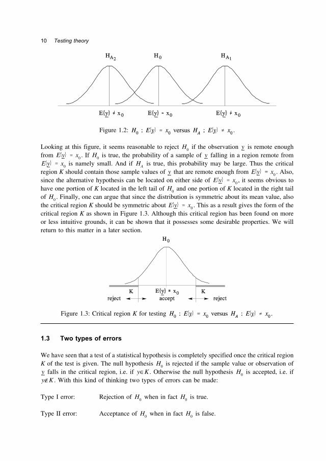
what values for rejecting . If a choice has been made of the values of that will correspondH0 yto rejection, then the remaining values of will necessarily correspond to acceptance. As definedyabove, the rejection values of constitute the critical region K of the test. Figure 1.2 shows theydistribution of under and under two possible alternatives and .y H0 HA1

HA2

10 Testing theory

Figure 1.2: .

Looking at this figure, it seems reasonable to reject if the observation is remote enoughH0 yfrom . If is true, the probability of a sample of falling in a region remote fromE y x0 H0 y

is namely small. And if is true, this probability may be large. Thus the criticalE y x0 HA

region K should contain those sample values of that are remote enough from . Also,y E y x0

since the alternative hypothesis can be located on either side of , it seems obvious toE y x0

have one portion of K located in the left tail of and one portion of K located in the right tailH0

of . Finally, one can argue that since the distribution is symmetric about its mean value, alsoH0

the critical region K should be symmetric about . This as a result gives the form of theE y x0

critical region K as shown in Figure 1.3. Although this critical region has been found on moreor less intuitive grounds, it can be shown that it possesses some desirable properties. We willreturn to this matter in a later section.

Figure 1.3: Critical region K for testing

1.3 Two types of errors

We have seen that a test of a statistical hypothesis is completely specified once the critical regionK of the test is given. The null hypothesis is rejected if the sample value or observation ofH0

falls in the critical region, i.e. if . Otherwise the null hypothesis is accepted, i.e. ify y∈K H0

. With this kind of thinking two types of errors can be made:y∉K

Type I error: Rejection of when in fact is true.H0 H0

Type II error: Acceptance of when in fact is false.H0 H0

Basic concepts of hypothesis testing 11

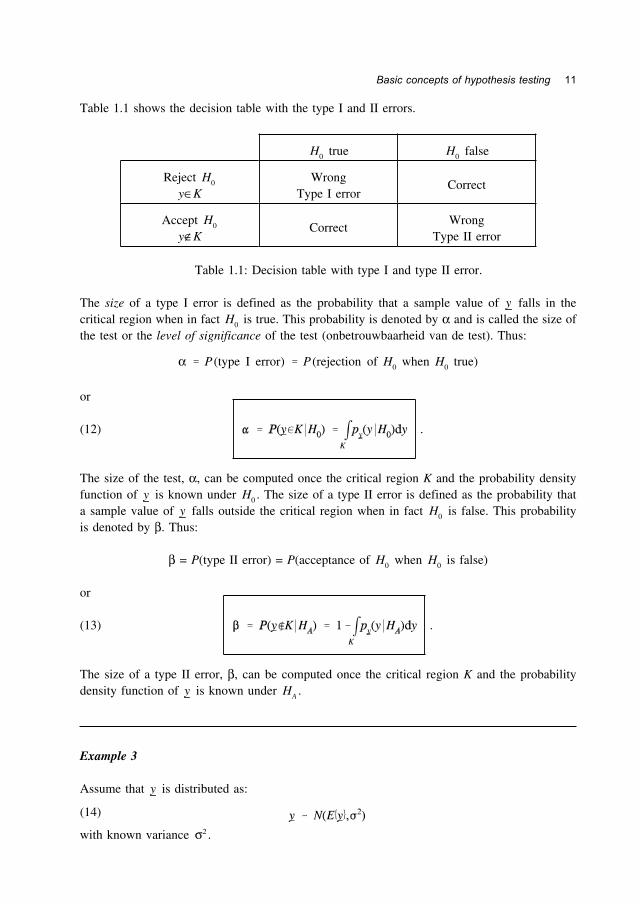
Table 1.1 shows the decision table with the type I and II errors.

trueH0 falseH0

Reject H0

y∈KWrong

Type I errorCorrect

Accept H0

y∉KCorrect

WrongType II error

Table 1.1: Decision table with type I and type II error.

The size of a type I error is defined as the probability that a sample value of falls in theycritical region when in fact is true. This probability is denoted by α and is called the size ofH0

the test or the level of significance of the test (onbetrouwbaarheid van de test). Thus:

or

α P (type I error) P (rejection of H0 when H0 true)

(12) .

The size of the test, α, can be computed once the critical region K and the probability densityfunction of is known under . The size of a type II error is defined as the probability thaty H0

a sample value of falls outside the critical region when in fact is false. This probabilityy H0

is denoted by β. Thus:

β = P(type II error) = P(acceptance of when is false)H0 H0

or

(13) .

The size of a type II error, β, can be computed once the critical region K and the probabilitydensity function of is known under .y HA

Example 3

Assume that is distributed as:y

with known variance .

(14)

σ2

12 Testing theory

The following two simple hypotheses are considered:

and

(15)

The situation is sketched in Figure 1.4.

(16)

Figure 1.4: The two simple hypotheses:

Since the alternative hypothesis is located on the right of the null hypothesis , it seemsHA H0

intuitively appealing to choose the critical region K right-sided. Figure 1.5a and 1.5b show twopossible right-sided critical regions K.

Figure 1.5: Critical region K and size of test, α.

They also show the size of the test, α, which corresponds to the area under the graph of thedistribution of under for the interval of the critical region K.y H0

Basic concepts of hypothesis testing 13

The size of the test, α, can be computed once the probability density function of under isy H0

known and the form and location of the critical region K is known. In the present example theform of the critical region has been chosen right-sided. Its location is determined by the valueof , the so-called critical value (kritieke waarde) of the test. Thus, for the present example thekαsize of the test can be computed as:

or, since:

as:

When one is dealing with one-dimensional normally distributed random variables, one can

(17)

usually compute the size of the test, α, from tables given for the standard normal distribution(see appendix B). In order to compute (17) with the help of such a table, we first have to applya transformation of variables. Since is normally distributed under with mean andy H0 x0

variance , it follows that the random variable , defined as:σ2 z

is standard normally distributed under . And since:

(18)

H0

we can use the last expression of (19) for computing α. Application of the change of variables

(19)

(18) to (17) gives:

We can now make use of the table of the standard normal distribution. Table 1.2 shows some

(20)

typical values of the α and for the case that .kα x0 1 and σ 2

14 Testing theory

αkα x0

σkα

0.10.050.010.001

1.281.652.333.09

3.564.295.657.18

Table 1.2: Test size α, critical value for and .kα x0 1 σ 2

As we have seen the location of the critical region K is determined by the value chosen for ,kαthe critical value of the test. But what value should we choose for ? Here the geodesist shouldkαbase his judgement on his experience. Usually one first makes a choice for the size of the test,α, and then by using (20) or Table 1.2 determines the corresponding critical value . Forkαinstance, if one fixes α at α = 0.01, the corresponding critical value (for the present examplekαwith ) reads The choice of α is based on the probability of a typex0 1 and σ 2 kα 5.65.I error one is willing to accept. For instance, if one chooses α as α = 0.01, one is willing toaccept that 1 out of a 100 experiments leads to rejection of when in fact is true.H0 H0

Let us now consider the size of a type II error, β. Figure 1.6 shows for the present example thesize of a type II error, β. It corresponds to the area under the graph of the distribution of yunder for the interval complementary to the critical region K.HA

Figure 1.6: The sizes of type I and type II error, α and β, for testing.H0: E y x0 versus HA: E y xA >x0

The size of a type II error, β, can be computed once the probability density function of undery HA

is known and the critical region K is known. Thus, for the present example the size of the typeII error can be computed as:

or since:

Basic concepts of hypothesis testing 15

as:

(21)

Also this value can be computed with the help of the table of the standard normal distribution.But first some transformations are needed. It will be clear that the probability that a sample orobservation of falls in the critical region K when is true, is identical to 1 minus they HA

probability that the sample does not fall in the critical region when is true. Thus:HA

(22)

Since for the present example:

substitution into (22) gives:

(23)

This formula has the same structure as (17). The value 1−β can therefore be computed in exactlythe same manner as the size of the test, α, was computed. And from 1−β it is trivial to computeβ, the size of the type II error.

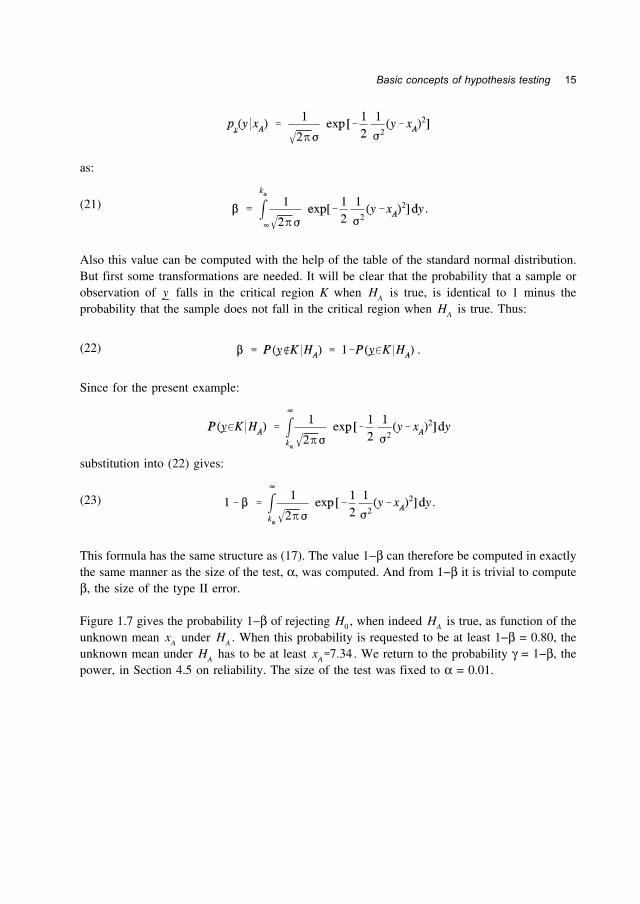
Figure 1.7 gives the probability 1−β of rejecting , when indeed is true, as function of theH0 HA

unknown mean under . When this probability is requested to be at least 1−β = 0.80, thexA HA

unknown mean under has to be at least . We return to the probability γ = 1−β, theHA xA 7.34power, in Section 4.5 on reliability. The size of the test was fixed to α = 0.01.

16 Testing theory

1 2 3 4 5 6 7 8 9 100

0.1

0.2

0.3

0.4

0.5

0.6

0.7

0.8

0.9

1

xA

pow

erγ=

1−β

Fig. 1.7: Probability γ = 1−β as function of , for testingxA

, with and .H0: E y x0 versus HA: E y xA >x0 x0 1 σ 2

1.4 A testing principle

We have seen that two types of errors are involved when testing a null hypothesis againstH0

an alternative hypothesis : (1) The rejection of when in fact is true (type I error); (2)HA H0 H0

the acceptance of when in fact is false (type II error). One might reasonably use the sizesH0 H0

of the two types of errors, α and β, to set up criteria for defining a best test. If this is possible,it would automatically give us a method of choosing a critical region K. A good test should bea test for which α is small (ideally 0) and β is small (ideally 0). It would therefore be nice if wecould define a test, i.e. define a critical region K, that simultaneously minimizes both α and β.Unfortunately this is not possible. As we decrease α, we tend to increase β, and vice versa. TheNeyman-Pearson principle provides a workable solution to this situation. This principle says thatwe should fix the size of the type I error, α, and minimize the size of the type II error, β. Thus:

A testing principle (Neyman et al., 1933): Among all tests or critical regions possessing the samesize type I error, α, choose one for which the size of the type II error, β, is as small as possible.

The justification for fixing the size of the type I error to be α, (usually small and often taken as0.05 or 0.01) seems to arise from those testing situations where the two hypotheses, ,H0 and HA

are formulated in such a way that one type of error is more serious than the other. Thehypotheses are stated so that the type I error is the more serious, and hence one wants to becertain that it is small. Testing principles other than the above given one can of course easily besuggested: for example, minimizing the sum of sizes of the two types of error, α + β. However,the Neyman-Pearson principle has proved to be very useful in practice. In this book we willtherefore base our method of finding tests on this principle. Now let us consider a testingproblem from the point of view of the Neyman-Pearson principle.

Basic concepts of hypothesis testing 17

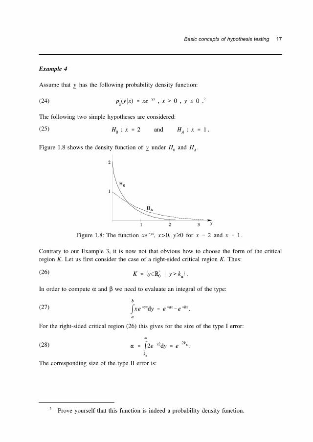
Example 4

Assume that has the following probability density function:y

(24) .2

The following two simple hypotheses are considered:

(25)

Figure 1.8 shows the density function of under .y H0 and HA

Figure 1.8: The function .xe yx, x>0, y≥0 for x 2 and x 1

Contrary to our Example 3, it is now not that obvious how to choose the form of the criticalregion K. Let us first consider the case of a right-sided critical region K. Thus:

In order to compute α and β we need to evaluate an integral of the type:

(26)

For the right-sided critical region (26) this gives for the size of the type I error:

(27)

The corresponding size of the type II error is:

(28)

2 Prove yourself that this function is indeed a probability density function.

18 Testing theory

Now let us consider a left-sided critical region as alternative. Thus:

(29)

K

For this critical region the size of the type I error becomes:

(30)

And the corresponding size of the type II error is given by:

(31)

Let us now compare the two tests, that is, the one with the right-sided critical region K with the

(32)

one with the left-sided critical region . We will base this comparison on the Neyman-PearsonKprinciple. According to this principle, both tests have the same size of type I error. Thus:

(33)

With (28) and (31) this gives or:

Using (29) and (32) this equation can be expressed in terms of and β as:

(34)

β

Hence:

Figure 1.9 shows the graph of this function. It clearly shows that:

(35)

(36)

The conclusion reads therefore that of the two tests the one having the right-sided critical regionK is the best in the sense of the Neyman-Pearson principle.

Basic concepts of hypothesis testing 19

Figure 1.9: The function .β (2β β2)1

2

1.5 General steps in testing hypotheses

Thus far we have discussed the basic concepts underlying most of the hypothesis-testingproblems. The same concept and guidelines will provide the basis for solving more complicatedhypothesis-testing problems as treated in the next chapters. Here we summarize the main stepson testing hypotheses about a general probability model.

(a) From the nature of the experimental data and the consideration of the assertions that areto be examined, identify the appropriate null hypothesis and alternative hypothesis:

(b) Choose the form of the critical region K that is likely to give the best test. Use theNeyman-Pearson principle to make this choice.

(c) Specify the size of the type I error, α, that one wishes to assign to the testing process.Use tables to determine the location of the critical region K from:

(d) Compute the size of the type II error:

to ensure that there exists a reasonable protection against type II errors.

(e) After the test has been explicitly formulated, determine whether the sample or observationy of falls in the critical region K or not. Reject if , and accept if .y H0 y∈K H0 y∉KNever claim however that the hypotheses have been proved false or true by the testing.