Texture-Based Visualization of Uncertainty in Flow Fields

Ralf P. Botchen1 Daniel Weiskopf1,2 Thomas Ertl1

1University of Stuttgart∗ 2Simon Fraser University

Figure 1: Three different advection schemes applied to a PIV measurement of a fluid flow data set. Left image: Gaussian error diffusionapproach. Center image: Cross advection method. Right image: Semi-Lagrangian advection using multi-frequency noise.

ABSTRACT

In this paper, we present two novel texture-based techniques to vi-sualize uncertainty in time-dependent 2D flow fields. Both meth-ods use semi-Lagrangian texture advection to show flow directionby streaklines and convey uncertainty by blurring these streaklines.The first approach applies a cross advection perpendicular to theflow direction. The second method employs isotropic diffusion thatcan be implemented by Gaussian filtering. Both methods are de-rived from a generic filtering process that is incorporated into thetraditional texture advection pipeline. Our visualization methodsallow for a continuous change of the density of flow representa-tion by adapting the density of particle injection. All methods canbe mapped to efficient GPU implementations. Therefore, the usercan interactively control all important characteristics of the sys-tem like particle density, error influence, or dye injection to cre-ate meaningful illustrations of the underlying uncertainty. Eventhough there are many sources of uncertainties, we focus on un-certainty that occurs during data acquisition. We demonstrate theusefulness of our methods for the example of real-world fluid flowdata measured with the particle image velocimetry (PIV) technique.Furthermore, we compare these techniques with an adapted multi-frequency noise approach.

CR Categories: I.3.3 [Computer Graphics]: Picture / Image Gen-eration I.3.6 [Computer Graphics]: Methodology and TechniquesI.3.8 [Computer Graphics]: Applications

Keywords: Uncertainty visualization, unsteady flow visualization,texture advection, GPU programming.

1 INTRODUCTION

Exposing uncertainties of real-world flow data becomes a more andmore important topic in the field of vector field visualization. Engi-neers and scientists are increasingly interested in which region andextent uncertainties occur in measured data. The absence of thisinformation can lead to wrong conclusions and therefore affect theanalysis process in a negative way. Several types of uncertainties orerrors can appear on the way from data acquisition to the final step

∗{botchen|weiskopf|ertl}@vis.uni-stuttgart.de

of visualization [11, 14, 24]. In this work, we focus on errors thatarise during the measurement step by inaccuracies of the measuringdevice or technique. Although scientists and engineers are aware ofthe fact that almost every data set has intrinsic uncertainties, mostvisualization techniques neglect or completely ignore them. Onereason for this is the difficulty to find a good uncertainty represen-tation that can be combined with the visualization of the originaldata. By including the error measure into the process of visualiza-tion we need to add one more variate. For one-dimensional data,uncertainty can be displayed by a traditional plot that shows the av-erage, minimum, and maximum value of a data point mapped to thesecond dimension. For multivariate data, this mapping becomes achallenging problem, since several dimensions have to be mappedto 2D screen space.

The goal of this paper is to provide new texture-based visual-ization schemes that do not only represent particle positions alongstreaklines but also bring out measuring errors and their influenceon particles in the form of smeared-out visual structures perpendic-ular to the flow direction. We adopt traditional semi-Lagrangiantexture advection [8, 19, 22], as briefly described in Section 4, andextend it by an error-dependent additional filter process that revealsuncertainty by essentially changing the spatial distribution of visualpatterns perpendicular to the flow. This generic error visualizationstrategy is introduced in Section 5. We have developed two spe-cific visualization methods that are derived from this generic strat-egy: First, the cross advection method, which uses a line-orientedfilter perpendicular to the flow direction (Section 6); second, anartificial error-guided diffusion filter (Section 7). Our visualiza-tion methods lend themselves to efficient GPU (graphics process-ing units) implementations, which is demonstrated by providing de-tails of the implementation along with performance measurements.Moreover, we compare our new methods with an adaptation of themulti-frequency noise method [9] and show results of uncertaintyvisualization applied to real-world fluid flow data from PIV mea-surements (see Section 9).

2 PREVIOUS WORK

Previous work on uncertainty visualization has focused on repre-senting uncertainty in simulation or analytical data. For example,Lodha et al. [12] evaluate and compare the quality of surface inter-polants and introduced geometric uncertainty as a measure of inter-polation error. Furthermore, they propose UFLOW [11], a systemto visualize uncertainties in streamlines of fluid flow with glyphs,

envelopes, or animation. Wittenbrink et al. [24] present several dif-ferent glyphs like uncertainty glyphs and arrow glyphs to visual-ize wind and ocean currents. They map uncertainty direction andmagnitude to various types of glyphs and glyph attributes. Pang etal. [14] give a classification of possibilities for visualizing uncer-tainties for a wide field of applications. Two techniques for uncer-tainty visualization in isosurface rendering are proposed by Rhodeset al. [16]. The first one changes one of the vertex color parametershue, saturation, or brightness. The second technique maps an ad-ditional texture on top of the surface and varies the opacity of thetexture according to the error measure. Finally, Brown [1] intro-duces a method of visual vibrations to indicate the amount of error.

Measurement of real-world data is a typical source of error oruncertainty. A widely used technique to acquire the velocity fieldof a fluid flow is based on particle image velocimetry (PIV) [6, 15].Since the quality and field of application of PIV measurements hasimproved in recent years, the analysis of PIV data is becoming in-creasingly interesting. For example, the recent work by Ebling etal. [3] applies image-processing methods to analyze PIV measure-ments.

Research in the field of texture-based flow visualization has beenstrongly advanced lately, not only because of the rapidly increas-ing performance and functionality of GPUs. The availability ofdense noise-based and sparse dye-based representations, as well asthe possibility for the user to interact and manipulate all impor-tant parameters on-the-fly also play an important role. The state-of-the-art in texture-based flow visualization is surveyed by Larameeet al. [10]. Early work on texture-based methods comprises spotnoise [18], line integral convolution (LIC) [2], and texture advec-tion [13]. More recent 2D techniques rely on semi-Lagrangian tex-ture advection: Image Based Flow Visualization (IBFV) by VanWijk [19] and Lagrangian-Eulerian Advection (LEA) by Jobard etal. [8]. Since dense texture representations need a large number ofcomputations, graphics hardware can improve the performance of2D texture-based flow visualization [5, 7, 23]. An example for asparse representation is the metaphor of dye advection [21, 22].

3 PARTICLE IMAGE VELOCIMETRY

Real-world fluid flow can be measured by particle image velocime-try (PIV) [6, 15]. The basic principle of PIV is to inject particlesinto the flow and to measure the movement of these particles be-tween two light pulses. Usually, a planar laser light sheet techniqueis used. In very short intervals the target area is illuminated twiceby a double-pulsed laser and recorded onto the CCD array of a dig-ital camera (see Figure 2). Since the CCD chip must be able tocapture each light pulse in separate image frames, the resolution intime is bound to the image frequency of the camera. Afterwards,appropriate algorithms evaluate consecutive images and determinethe displacement of particles in the flow. The most common wayof measuring displacement is to divide the image plane into smallinterrogation areas (IA) and cross correlate the images from the twotime exposures. With this method, even unsteady or non-periodicflow fields can be measured.

One possible cross correlation algorithm works as follows: Eachimage is divided into l small IAs with edge length K (in pixels);the IAs are then shifted and compared with other parts of the im-age. For each translation ∆x of one IA A with K2 pixels to anotherdomain B of the same size, the cross correlation

C(∆x) =K

∑i=1

K

∑j=1

Bi j ·Ai j(∆x) (1)

can be computed. If the coefficient C is a maximum and/or mini-mum for a translation ∆x (depending on the matrix function), then

CCD

array

lens

lens

light

sheet

target

area

flow with

particles

∆t

∆AI

image

frame timage

frame t+∆t

X

correlation

vector field

double-

pulsed

laser

Figure 2: Configuration of a particle image velocimetry system.

the largest match between A and B and thus the shift of the parti-cles has been found for IA A. Solving Eq. (1) for all IAs ∆xl ofthe image results in a collection of displacement vectors that can beconverted to velocity vectors by using the time difference betweenboth evaluated images:

vl(xl) =dxl

dt≈

∆xl

t2 − t1.

On the way from data acquisition to the stage of visualization, sev-eral different uncertainties or errors can be introduced to the data[11, 14]. Figure 3 shows the three stage pipeline that data has to

data acquisition transformation visualization

simulation

database

sensors

sampling

quantization

interpolation

volume

flow

animation

analysis

data

uncertainty

derived

uncertainty

visualization

uncertainty

Figure 3: Possible sources for uncertainties (adopted from [14]).

go through until it can be analyzed. In the visualization step, al-gorithmic uncertainties can occur, e.g., by approximating factorsfor global illumination or by interpolating data values on slices involume rendering. Transformation uncertainties are introduced byconverting from one unit to another or by scaling, resampling, orquantization. In our work, we focus on uncertainties that appearin the first stage—during data acquisition. We think that this stageis most interesting for uncertainty visualization because the errorsfrom data acquisition typically cannot be influenced or reduced bysubsequent processes. In contrast, algorithmic or numerical errorsfrom the other two stages of the pipeline can be neglected if algo-rithms of appropriate quality are applied. Nevertheless, error fromany source could be used as input to, and thus shown by, our uncer-tainty visualization methods.

During data acquisition, errors can be introduced into PIV datasets from several sources [15]:

• Random error due to noise in the recorded images.• Bias error arising from the process of computing the signal

peak location to sub-pixel accuracy.• Calibration inaccuracy of the CCD camera.

• Acceleration error caused by approximating the local Eulerianvelocity from the Lagrangian motion of tracer particles.

• Gradient error resulting from rotation and deformation of theflow within an interrogation area leading to a loss of correla-tion.

• Dimension of the cross-correlated interrogation areas.• Tracking error resulting from the inability of a particle to fol-

low the flow without slip.

Some of these errors can be minimized by carefully choosing theexperimental conditions, but others cannot be eliminated and thusthe final data inherits uncertainties by the nature of the measuringsystem. Since engineers are fully aware of the existence of thoseuncertainties it can be of great advantage to have an interactive vi-sual feedback during analysis.

In our system, the PIV method yields N measurements for thevector field at each spatial location and time step. The raw datameasurements are denoted vi with i = 1 . . .N. The average vectorv serves as basis for traditional vector field visualization. Then, theroot mean square

rrms =

√

√

√

√

1N

N

∑i=1

||vi −v||2 ,

can be used as the measure of uncertainty.Our test data set was acquired in a laminar water channel with

a 3D S-PIV method and a resolution of 81 × 45 in each of nineseparated layers. Each layer was measured N = 25 times. Since ourcomputation takes place in the 2D domain, we slice the 3D vectorfield into nine separated 2D layers.

4 SEMI-LAGRANGIAN TEXTURE ADVECTION

Texture advection is a well-established and versatile method forvisualizing unsteady flow [8, 13, 19]. Semi-Lagrangian transport[8, 17], which is the basis for our implementation of texture advec-tion, is briefly described in this section.

Particles or injected dye are represented on a regularly sampledgrid or texture. This property field is denoted by ρ(x). The pointsx are from the domain of the nD vector field, R

n. For the Eulerianapproach, particles lose their individuality and their position is im-plicitly given by the location of the corresponding texel in the prop-erty field. Particles are transported along streamlines for steady, oralong pathlines for unsteady vector fields v(x, t), where t denotestime. The Lagrangian formulation of the underlying equation ofmotion,

dx(t)dt

= v(x(t), t) ,

can be integrated to compute the pathline of an advected masslessparticle,

x(t1) = x(t0)+∫ t1

t0v(x(t), t)dt . (2)

The evolution of the property field ρ(x, t) is governed by

∂ρ(x, t)∂ t

+v(x, t) ·∇ρ(x, t) = 0 .

This partial differential equation can be solved by semi-Lagrangiantransport [8, 17], which leads to a stable evolution even for largestep sizes. A backward texture lookup is often employed:

ρ(x(t0), t0) = ρ(x(t0 −∆t), t0 −∆t) . (3)

Starting from the current time step t0, an integration backwards intime according to Eq. (2) provides the position at the previous time

step, x(t0 −∆t). Texture-based methods often produce only shortstreamlines or streaklines and, therefore, first-order Euler integra-tion typically provides sufficient accuracy:

x(t0 −∆t) = x(t0)−∆tv(x(t0), t0) .

The property field is evaluated at this previous position to access theparticle that is transported to the current position. Tensor-productlinear interpolation (bilinear in 2D or trilinear in 3D) is applied toreconstruct the property field at locations different from grid points.

Texture advection can be used to visualize larger structures in theflow, like streamlines in steady flow or streaklines in time-varyingflow. These structures can be generated by injecting smooth dyepatterns or noise-based particles into the property field ρ after eachadvection step, following the IBFV approach [19]. Newly injectedmaterial is combined with the advected property field by means ofalpha blending, which represents the discretized version of an ex-ponential filter kernel [4] in the context of LIC [2]. We use textureadvection as basis for uncertainty visualization because it offers im-portant benefits. First, the injection scheme is flexible in allowingthe user to gradually change the density of new particles from a fewrandomly injected particles up to a densely filled property field rep-resented by white noise. Second, texture advection lends itself to adirect and efficient mapping to GPUs, which leads to an interactivevisualization of large data sets.

5 STRATEGY FOR UNCERTAINTY VISUALIZATION

The goal of this paper is to enrich texture advection by a visual-ization of flow uncertainty, without losing the benefits of textureadvection, i.e., its flexibility and efficiency. Uncertainty visualiza-tion essentially requires to represent one additional single-valuedattribute: a measure for uncertainty or error.

From an abstract point of view, uncertainty visualization can bestructured into a three-stage process (see Figure 4). Raw data is

original error

measurederived error

measure

visual

representationraw data

combination

e.g. rms

functional

mapping

visual

mapping

Figure 4: Uncertainty pipeline.

the basis to compute an error value. As detailed in Section 3, theerror value for PIV data is typically based on the root mean square.However, any other error computation could be used for this partof the visualization process. In the second stage, this original errorvalue is mapped to a derived error measure, e.g., by a linear or anon-linear function, in order to obtain values in a useful range. Wedenote this, possibly space-variant and time-dependent, uncertaintymeasure by u(x, t). The third step comprises the actual mappingto visual primitives. This step is the main objective of uncertaintyvisualization.

Various means of a visual mapping of multi-variate data could beemployed to represent the error attribute. A simple and well-knownmethod is to map the derived error value to color and to overlay thiscolor on top of the underlying flow visualization. However, thiskind of visualization method only shows uncertainty at a respectivepoint, i.e., it results in a localized representation. In contrast, uncer-tainty in a flow leads to an uncertainty of particle transport, whichshould also be represented by means of “uncertain” particle traces.It is reasonable to mark a particle that has been advected throughoutan error-affected area and to emphasize this in the further process ofthe flow. Furthermore, an uncertainty-affected region can influence

texture advection

particle and

dye injection

error advection

load flow and

error data

display

initialize

property field

next tim

e s

tep

Figure 5: Flowchart of the algorithm.

its neighborhood and this should be taken into account in the visu-alization step. Therefore, our goal is to incorporate the uncertaintyrepresentation within the concept of texture-based particle trans-port. Another advantage of this approach is that the error attributeis encoded in the same perceptual channel as the original flow—inthe form of a texture—and, thus, other perceptual channels (e.g.,color) could be used to encode additional attributes.

We propose the following basic visualization process that com-bines uncertainty visualization with traditional texture advection.As laid out in Figure 5, the first steps of the visualization cycle(”load flow data”, ”texture advection”, and ”particle and dye in-jection”) are identical to traditional texture advection. Uncertaintyvisualization is exclusively based on an additional error filteringstage, that is completely decoupled from the texture advection com-putation. Error filtering aims at manipulating the spatial frequencyperpendicular to particle traces to show uncertainty u(x, t), i.e., wedo not only change the spatial frequency along the flow as in LIC [2]or basic texture advection [10].

Error filtering modifies the property field and, in its generic form,can be formulated as

ρfiltered(x) =∫

V (x,v)

f (u, x,v)ρ(x+ x)dnx . (4)

The compact nD filter domain V (x,v) may be space-variant andflow-dependent, and so is the filter f . The integral is evaluated ata fixed time t. In this paper, we restrict ourselves to 2D visualiza-tion with n = 2 and we use two special cases for Eq. (4), whichare detailed in Sections 6 and 7. Different “flavors” of uncertaintyvisualization are achieved by choosing specific parameters for thefilter kernel and integration domain.

6 CROSS ADVECTION

Cross advection is the first specific example for error filtering. Here,the filter domain is reduced to a line perpendicular to the currentflow direction. The fundamental idea is to transport a particle lat-erally to the flow direction and thus smear out the streakline of theparticle. This essentially leads to a 1D convolution similar to thatof traditional texture advection. The only difference is that a sym-metric filter (in both directions) is applied.

Discretization of the filter leads to

ρfiltered = ∑i∈{−1,0,1}

fiρi , (5)

where fi is the discrete filter kernel and ρi are samples of the prop-

advection

time step t-∆t time step t

error region

error region

transp

ort

ρc

ρ-γ

ργ

transp

ort

Figure 6: Semi-Lagrangian transport of a particle along flow directioninto an error region from time step t−∆t to time step t. The crossadvection is applied in time step t.

erty field along the perpendicular line,

ρi = ρ(x+ iµ∆tMrotv(x, t)) . (6)

Here, µ denotes the error-depending relative step size, ∆t is the stepsize of traditional texture advection, and Mrot is a 2D matrix for arotation by 90 degrees. The integration width and, thus, the lengthscale for smearing is controlled by the error value via µ . Equa-tion (5) implements the analog of line integral convolution basedon texture advection, with the following differences: First, a con-volution perpendicular to the flow direction is performed; second, asymmetric convolution filter in both directions is applied. This fil-tering maintains a constant overall brightness if a normalized kernelis used (i.e., ∑ fi = 1). A typical choice is fi = 0.25,0.5,0.25.

Figure 6 illustrates the two steps performed for the completecross advection approach. In the first step, a particle (grey dot)is transported by traditional semi-Lagrangian advection along theflow direction into an uncertainty region. Black grid points lie in-side the error region, white grid points outside. In the next stepshown on the right side of Figure 6, we compute the intensity val-ues of the current point (grey dot) and the two cross directionalpoints (white and black dots) by combining the values according toEq. (5).

The filtering process can be slightly modified by replacing theweighted sum in Eq. (5) by a maximum function according to

ρfiltered = max{ρi|i = 1,2,3} . (7)

The max() function guarantees that (sparsely seeded) streaklinesare not reduced to very small intensities in regions of large error,and therefore smeared-out streaklines are maintained. In general,the max() function does not provide a constant overall brightnessbut tends to increase the image brightness. Therefore, this variantis primarily designed for sparse representations with a few, clearlyseparated streaklines.

Cross advection can be considered an image-processing opera-tion that can be directly mapped to GPU fragment operations. Theupdate equations (5) or (7) work independently on 2D grid cells ofthe property field. By identifying this 2D grid with a texture, theupdate of cells (i.e., texels) is reduced to updating the underlyingtexture through a fragment program. In fact, ping-pong renderingis employed to update textures: Two copies of the property fieldare held in texture memory; one serves as render target, the otherone serves as input texture. After each update, the role of the twotextures is exchanged. This cross advection process is one examplefor an ”error advection module” in Figure 5.

Figure 7: Left image: Cross advection with a single dye pattern ina laminar flow field and with piecewise constant uncertainty. Rightimage: Sparsely injected particles into the same flow with increasinguncertainty from top to bottom.

A HLSL fragment program of the basic transport mechanism forEq. (7) is given in Figure 8. The mapping from the input uncertaintymeasure to the relative step size µ is implemented by a dependent-texture lookup. The space-variant input uncertainty is held in a 2Ddomain-filling texture. We need to perform three texture lookups inthe property texture to evaluate Eq. (6). In the 2D case, the rotationmatrix Mrot can be realized by a component swizzle followed bya simple multiplication. Finally, the texel with maximum intensityis written to the output. In a variant of this fragment program, themax() function is replaced by a weighted sum to implement Eq. (5).

The left image of Figure 7 shows an example of a single dyepattern injected into a uniform flow field. The underlying uncer-tainty begins a few steps away from the injection point and thenstays constant. The exact shape of the streakline is visible in theerror-free part of the flow that changes to a symmetric expansionof both sides. The right image illustrates a sparse injection of ran-dom particles, while the uncertainty increases from top to bottom.Since uncertainty magnitude effects the step size of cross transport,streaklines in regions with large errors (bottom) spread more thanthose in unaffected regions (top).

// lookup in all textures at current TexCoord position

float4 direction = tex2D( VectorField, TexCoord );

// result from previous traditional texture advection

float4 thistxl = tex2D( AdvectedTex, TexCoord );

// uncertainty measure u(x,t)

float error = tex2D( ErrorField, TexCoord );

// cross advection step size: mu * Delta t

float stepSize = tex2D( ErrorStepSize, error );

float4 maxintens;

// perform cross advection in both directions

direction.yx = direction.xy * stepSize.xx;

direction.x *= -1.0f; // rotate -90

newpos.xy = TexCoords - direction.xy;

float4 lefttxl = tex2D( AdvectedTex, newpos.xy );

newpos.xy = TexCoord + direction.xy; // rotate 180

float4 righttxl = tex2D( AdvectedTex, newpos.xy );

// find texel with maximum intensity

maxintens.x = max( lefttxl.x, righttxl.x );

maxintens.x = max( thistxl.x, maxintens.x );

// final output

Output.RGBA = maxintens.xxxx;

return Output;

Figure 8: Main part of the HLSL fragment program for the crossadvection approach.

Figure 9: Left image: Gaussian error diffusion with a single dye pat-tern in a laminar flow with piecewise constant uncertainty. Rightimage: Sparsely injected particles into the same flow, with uncer-tainty magnitude increasing from top to bottom.

7 ERROR DIFFUSION

Error diffusion is our second technique based on the generic fil-tering process from Eq. (4). In contrast to cross advection, errordiffusion applies an isotropic 2D filter kernel, independent of thedirection of the flow. Filtering is space-variant: The uncertaintyvalue determines the strength of smearing out. While cross advec-tion blurs the streakline sideways to the flow direction, the diffusionfilter affects texels not only in direction of the flow but in all direc-tions. Since an error-affected data point exerts influence to all itsadjacent points in real data measurements, this filtering process im-itates natural diffusion. A typical filter kernel is a 2D Gaussianfunction, normalized in order to maintain a constant brightness.We do not recommend to employ a max() function here becausethis would lead to an overly fast increase in brightness—due to thelarger support of the filter, there is a higher probability of collectingbright contributions than in the cross advection approach.

The diffusion computation is completely detached from the ad-vection step and can be computed separately as shown in Figure 5.In this second step, we apply a discretized 2D filter kernel to thepreviously advected particles. For a GPU implementation, it isinefficient to use a large filter kernel because this would increasethe computation costs dramatically. Therefore, we implementedonly a discrete, separated 3× 3 Gaussian filter. A larger filter ker-nel is achieved by successive application of this 3× 3 filter, wherethe number of filtering steps is determined by the extent of uncer-tainty. A fine-grained control of filter strength through the uncer-tainty value is achieved by modifying the entries in the filter mask.The actual filter is constructed from a linear interpolation betweenan identity mapping and a full Gaussian kernel, where the inter-polation weight is determined by the uncertainty value. Linear in-terpolation guarantees that the integral over the interpolated filterremains constant and normalized. In this way, we are able to obtainare range of filtering results, all the way from an identity mappingin regions with no uncertainty (which results in exact streaklines)up to a standard Gauss filter in regions with maximum uncertainty(which strongly blurs the streakline in all directions). For the GPUimplementation, both the identity mapping and the Gaussian func-tion are held in a floating-point texture. During runtime we performa bilinear lookup in this texture and compute the linear interpolationto obtain a modified filter kernel.

The left image of Figure 9 illustrates dye injected into a lam-inar flow field with constant uncertainty, beginning a few stepsaway from the injection point. Well recognizable is the one-to-onemapping of the streakline in areas without error influence, whichchanges to a constant blurring in all directions in the error-affectedregion. The right image shows the Gaussian error diffusion ap-proach applied to sparsely injected particles into the same flow with

Figure 10: Comparison of cross advection and Gaussian error dif-fusion with two dye patterns injected into a flow with increasinguncertainty from left to right.

increasing uncertainty from top to bottom. This picture illustratesthat the size and weight of the filter kernel depend on the uncer-tainty magnitude; hence streaklines in the lower part of the flow areheavily blurred while streaklines in the upper part are mapped toidentity. Figure 10 shows both approaches with two injected dyepatterns into a laminar flow field with increasing uncertainty fromleft to right. Considering the lower dye in the left image, one cansee how uncertainty magnitude affects the step size of the crossadvection and how the streakline widens due to an increasing stepsize. Depending on the 2D convolution kernel, the wavefront of astreakline computed with the error diffusion approach, runs fasterthan traditional texture advection or the cross advection approach.

8 MULTI-FREQUENCY NOISE

We adopt the generic multi-frequency noise approach [9] as thirdtechnique for a dense vector field representation. Here, uncertaintyis used to control the spatial frequency of noise injection. Thistechnique can be directly incorporated into semi-Lagrangian ad-vection by slightly modifying the injected noise. The original 2Dnoise is replaced by a 3D noise texture whose layers are filled withnoise patterns of varying maximum spatial frequency. The first slicecontains original white noise; all successive slices contain filteredversions of this white noise with decreasing maximum frequency.Filtering is based on the fast Fourier transform: First, the originalwhite noise is transformed to frequency space, then a low pass fil-ter is applied in frequency space and finally we perform the inverseFourier transformation back to image space. Since low-pass filteredimages lose contrast, we apply histogram equalization to match thecontrast of the original image and sharpen the low-frequency struc-tures. To access the different layers, the noise lookup is extendedby a third dimension that is controlled by the error value. Figure 11gives an example of four different noise patterns and their applica-tion to the visualization of a uniform flow field.

9 DISCUSSION AND RESULTS

In Sections 6–8, we have discussed three different techniques tovisualize uncertainties in vector fields. All methods are suitablefor a dense representation and manipulate the spatial frequency ac-cording to the uncertainty value. Multi-frequency noise is a pre-filtering method—all necessary spatial frequencies have to be pre-computed and stored in a 3D texture. Our novel approaches applypost-processed filtering to the streaklines, and therefore, comparedto the multi-frequency approach, the results are similar for densenoise injection but differ drastically for a sparse injection. An im-portant advantage of both new methods is that they permit a contin-uous transition from a dense to a sparse representation, whereas the

Figure 11: Left image: Four layers of multi-frequency noise. Thefrequency depends on the uncertainty value. Right image: Advectionof multi-frequency noise in a laminar flow.

multi-frequency approach only works for a dense representation. Asparse noise injection or the injection of a smooth dye pattern al-lows the analyst to focus on single streaklines and their behavioraccording to the underlying flow field.

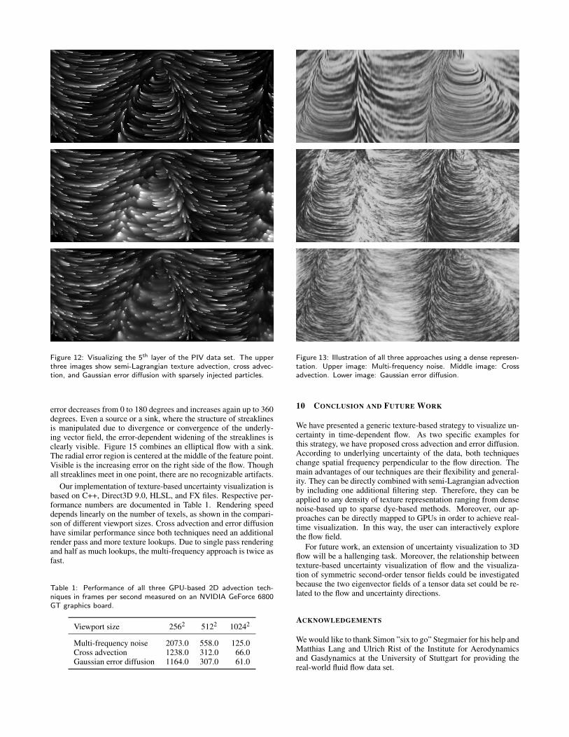
We illustrate all techniques on our test data set, which was mea-sured in a laminar water channel with the PIV method. This data setcontains one time step of water streaming through the test channel,producing vortices in the flow. The upper image of Figure 12 showsthe fifth layer of the data set. Clear streaklines are generated withtraditional semi-Lagrangian texture advection using alpha blendingas exponential filter along flow direction. Streaklines only widenin divergent parts of the vector field and due to numerical diffu-sion. The second image shows the same flow visualized with thecross advection approach. In regions with marginal uncertainty, thestreaklines remain clear but in uncertainty-affected regions they be-come blurred perpendicular to the flow by an extent that dependson the uncertainty value. The same applies to the third image, gen-erated by Gaussian error diffusion. With both techniques, the usercan still see structures of the flow in error regions, though the spa-tial frequency has been reduced. Furthermore, even the orientationof the flow is distinguishable due to the OLIC-like [20] structure ofthe streaklines.

For a sparse particle injection, the multi-frequency approach isnot suitable. We have not included a picture in Figure 12 for com-parison because low-pass filtering of sparse injected particles wouldlead to artifacts as known from heavy JPEG compressed images.Further, one would recognize single, isolated and large streaks, buttheir width would not change depending on uncertainty. Therefore,this approach is not intuitive enough for uncertainty visualization.Figure 13 directly compares our three uncertainty approaches by us-ing dense particle injection represented by a white noise pattern. Asanticipated, the spatial frequencies strongly decrease in regions oflarge error, irrespectively of the method being pre-filtered or post-filtered. All techniques produce similar results and eliminate struc-tures of the streaklines in error regions. Our new approaches canbe applied for dye patterns in the same way as for dense particletextures, which enables the engineer to interactively release dye ininteresting regions to explore features of the flow. Accompanyingvideo material can be found on the project web page1.

In Figures 14 and 15, we use two synthetically generated datasets to demonstrate the behavior of the uncertainty advection ap-proaches in regions of typical vector field features. Figure 14 showsthree different topological structures such as source, sink, and twovortices, visualized with the cross advection method. Each featurepoint has an artificial error applied. The value of the error region isindependent of the radius, but depends on the rotation angle. The

1 http://www.vis.uni-stuttgart.de/texflowvis/

uncertainties

Figure 12: Visualizing the 5th layer of the PIV data set. The upperthree images show semi-Lagrangian texture advection, cross advec-tion, and Gaussian error diffusion with sparsely injected particles.

error decreases from 0 to 180 degrees and increases again up to 360degrees. Even a source or a sink, where the structure of streaklinesis manipulated due to divergence or convergence of the underly-ing vector field, the error-dependent widening of the streaklines isclearly visible. Figure 15 combines an elliptical flow with a sink.The radial error region is centered at the middle of the feature point.Visible is the increasing error on the right side of the flow. Thoughall streaklines meet in one point, there are no recognizable artifacts.

Our implementation of texture-based uncertainty visualization isbased on C++, Direct3D 9.0, HLSL, and FX files. Respective per-formance numbers are documented in Table 1. Rendering speeddepends linearly on the number of texels, as shown in the compari-son of different viewport sizes. Cross advection and error diffusionhave similar performance since both techniques need an additionalrender pass and more texture lookups. Due to single pass renderingand half as much lookups, the multi-frequency approach is twice asfast.

Table 1: Performance of all three GPU-based 2D advection tech-niques in frames per second measured on an NVIDIA GeForce 6800GT graphics board.

Viewport size 2562 5122 10242

Multi-frequency noise 2073.0 558.0 125.0Cross advection 1238.0 312.0 66.0Gaussian error diffusion 1164.0 307.0 61.0

Figure 13: Illustration of all three approaches using a dense represen-tation. Upper image: Multi-frequency noise. Middle image: Crossadvection. Lower image: Gaussian error diffusion.

10 CONCLUSION AND FUTURE WORK

We have presented a generic texture-based strategy to visualize un-certainty in time-dependent flow. As two specific examples forthis strategy, we have proposed cross advection and error diffusion.According to underlying uncertainty of the data, both techniqueschange spatial frequency perpendicular to the flow direction. Themain advantages of our techniques are their flexibility and general-ity. They can be directly combined with semi-Lagrangian advectionby including one additional filtering step. Therefore, they can beapplied to any density of texture representation ranging from densenoise-based up to sparse dye-based methods. Moreover, our ap-proaches can be directly mapped to GPUs in order to achieve real-time visualization. In this way, the user can interactively explorethe flow field.

For future work, an extension of uncertainty visualization to 3Dflow will be a hallenging task. Moreover, the relationship betweentexture-based uncertainty visualization of flow and the visualiza-tion of symmetric second-order tensor fields could be investigatedbecause the two eigenvector fields of a tensor data set could be re-lated to the flow and uncertainty directions.

ACKNOWLEDGEMENTS

We would like to thank Simon ”six to go” Stegmaier for his help andMatthias Lang and Ulrich Rist of the Institute for Aerodynamicsand Gasdynamics at the University of Stuttgart for providing thereal-world fluid flow data set.

Figure 14: This synthetic data set combines different flow featureslike source, sink, and vortices to clarify the behavior of the crossadvection approach in critical regions.

REFERENCES

[1] R. Brown. Animated visual vibrations as an uncertainty visualisationtechnique. In Proc. GRAPHITE 2004, pages 84–89, 2004.

[2] B. Cabral and L. C. Leedom. Imaging vector fields using line integralconvolution. In Proc. ACM SIGGRAPH, pages 263–270, 1993.

[3] J. Ebling, G. Scheuermann, and B. G. van der Wall. Analysis and vi-sualization of 3-C PIV images from HART II using image processingmethods. In Eurovis 2005 (Eurographics / IEEE VGTC Symposiumon Visualization), pages 161–168, 2005.

[4] G. Erlebacher, B. Jobard, and D. Weiskopf. Flow textures: High-resolution flow visualization. In C. D. Hansen and C. R. Johnson,editors, The Visualization Handbook, pages 279–293. Elsevier, Ams-terdam, 2005.

[5] W. Heidrich, R. Westermann, H.-P. Seidel, and T. Ertl. Applications ofpixel textures in visualization and realistic image synthesis. In ACMSymposium on Interactive 3D Graphics, pages 127–134, 1999.

[6] K. D. Hinsch. Particle image velocimetry. In R. S. Sirohi, editor,Speckle Metrology, pages 235–324. Marcel Dekker, New York, 1993.

[7] B. Jobard, G. Erlebacher, and M. Y. Hussaini. Hardware-acceleratedtexture advection for unsteady flow visualization. In IEEE Visualiza-tion 2000, pages 155–162, 2000.

[8] B. Jobard, G. Erlebacher, and M. Y. Hussaini. Lagrangian-Eulerianadvection of noise and dye textures for unsteady flow visualiza-tion. IEEE Transactions on Visualization and Computer Graphics,8(3):211–222, 2002.

[9] M. Kiu and D. C. Banks. Multi-frequency noise for LIC. In IEEEVisualization ’96, pages 121–126, 1996.

[10] R. S. Laramee, H. Hauser, H. Doleisch, B. Vrolijk, F. H. Post, andD. Weiskopf. The state of the art in flow visualization: Dense andtexture-based techniques. Computer Graphics Forum, 23(2):143–161,2004.

[11] S. K. Lodha, A. Pang, R. E. Sheehan, and C. M. Wittenbrink.UFLOW: Visualizing uncertainty in fluid flow. In IEEE Visualization’96, pages 249–254, 1996.

[12] S. K. Lodha, B. Sheehan, A. T. Pang, and C. M. Wittenbrink. Vi-sualizing geometric uncertainty of surface interpolants. In GraphicsInterface ’96, pages 238–245, 1996.

Figure 15: Cross advection approach for the example of a syntheticdata set that combines a circular flow with a sink in the middle ofthe domain.

[13] N. Max and B. Becker. Flow visualization using moving textures.In Proc. ICASW/LaRC Symposium on Visualizing Time-Varying Data,pages 77–87, 1995.

[14] A. T. Pang, C. M. Wittenbrink, and S. K. Lodha. Approaches to un-certainty visualization. The Visual Computer, 13(8):370–390, 1997.

[15] A. Prasad. Particle image velocimetry. Current Science, 79(1):101–110, 2000.

[16] P. J. Rhodes, R. S. Laramee, R. D. Bergeron, and T. M. Sparr. Uncer-tainty visualization methods in isosurface rendering. In Eurographics2003 Short Papers, pages 83–88, 2003.

[17] J. Stam. Stable fluids. In Proc. ACM SIGGRAPH, pages 121–128,1999.

[18] J. J. van Wijk. Spot noise – texture synthesis for data visualization.Computer Graphics (Proc. ACM SIGGRAPH 91), 25:309–318, 1991.

[19] J. J. van Wijk. Image based flow visualization. ACM Transactions onGraphics, 21(3):745–754, 2002.

[20] R. Wegenkittl, E. Groller, and W. Purgathofer. Animating flow fields:Rendering of oriented line integral convolution. In Computer Anima-tion ’97, pages 15–21, 1997.

[21] D. Weiskopf. Dye advection without the blur: A level-set approachfor texture-based visualization of unsteady flow. Computer GraphicsForum (Proc. Eurographics 2004), 23(3):479–488, 2004.

[22] D. Weiskopf, R. P. Botchen, and T. Ertl. Interactive visualization of di-vergence in unsteady flow by level-set dye advection. In Proc. SimVis2005, pages 221–232, 2005.

[23] D. Weiskopf, M. Hopf, and T. Ertl. Hardware-accelerated visualiza-tion of time-varying 2D and 3D vector fields by texture advection viaprogrammable per-pixel operations. In Proc. VMV 2001, pages 439–446, 2001.

[24] C. M. Wittenbrink, A. T. Pang, and S. K. Lodha. Glyphs for visual-izing uncertainty in vector fields. IEEE Transactions on Visualizationand Computer Graphics, 2(3):266–279, 1996.