Page 1
International Journal of Combined Research & Development (IJCRD)
eISSN:2321-225X;pISSN:2321-2241 Volume: 4; Issue: 3; March -2015
www.ijcrd.com Page 6
Texture feature based Medicinal plant Recognition
Varuna Shree 1 N , Punitha.P
2
1,2 PES UNIVERSITY, 100-Ft. Ring Road,
BSK III Stage, Bangalore - 560085. [email protected] ,
[email protected]
ABSTRACT. In this paper we propose a methodology for the recognition of medicinal plant
images based on edge direction histogram and scale invariant feature transform. Manual
identification of medicinal plants requires lot of prior knowledge. Therefore it is necessary for
an automated system for recognizing plant species based on leaf images. The data set for
experimentation consists of 600 images divided into training and testing sets. We have used
optimal edge detection algorithm for detection of edges in leaves and the edge direction
histogram (EDH) features are extracted. For the extraction of the salient features in leaves, we
have used a Scale invariant feature transform (SIFT) algorithm. Finally these features are used
in retrieval of medicinal plant images. Matching between the extracted features is achieved
using Euclidean distance for EDH features and Distance ratio method for SIFT features.
Result shows which algorithm is efficient in retrieving each category of medicinal plant.
Keywords: Edge direction histogram, scale invariant feature transform.
1. INTRODUCTION
The forests in India are the principle resources of large number of medicinal plants which are widely
used in the preparation of ayurvedic medicine. Medicinal plants consist of components of therapeutic
values and have been used in medication of human diseases since long. Medicinal plants form the
backbone of system of medicine called Ayurveda and are useful in the treatment of certain chronic
diseases such as cancer, diabetes, blood pressure and skin problems. In rural and remote areas, more
than 70% of population depends on traditional system of medicines obtained from the medicinal plants.
The Indian system of medicine use around 8,000 species of plants which include trees (33%), herbs
(32%), shrubs (20%), climbers (12%) and epiphytes, grasses, lichens, ferns and algae put together (3%).
Among 2,000 drugs being used in curing human ailments in India, only 200 are of animal origin, 300 of
mineral origin and the rest 1500 drugs are extracted from various medicinal plants. Due to the
pathogenic resistance against the available antibiotics and the recognition of traditional medicine as an
alternative form of heath care has reopened the research domain for the biological activities of medicinal
plants.
A plant exists everywhere we live, around us. The lack of knowledge about medicinal plants and
modernization is posing serious threats to medicinal plants it has become very difficult to save plants
which serves as natural health boosters. There are many evidences where experts go in search of the
availability of these medicinal plants in forests which is a tedious and challenging task for any human
being. But in recent times, there has been an increasing awareness about the significance of medicinal
plants as people are returning to the ancient and traditional system of phyto-medicines.
We believe that the first step is to teach a computer how to recognize medicinal plants based on leaf
images of plants. One can easily transfer the image to a computer and computer can extract features
automatically using image processing techniques. Therefore, it is necessary to develop an automatic
Page 2
International Journal of Combined Research & Development (IJCRD)
eISSN:2321-225X;pISSN:2321-2241 Volume: 4; Issue: 3; March -2015
www.ijcrd.com Page 7
method that identifies the medicinal plants from their images using image processing techniques by
extracting features for identification, such as shape, color, texture. This automated recognition system
will prove extremely useful in quick and efficient way to correctly recognize medicinal plants of
different species.
The paper is organized into six sections. Section two gives image acquisition and details of the proposed
methodology. Section three describes the partition of image, feature extraction and feature matching.
Section four describes performance evaluation. The result and discussion are given in section five.
Section six gives conclusion of the work.
2. PROPOSED METHODOLOGY
2.1 Image Acquisition
The image samples of different plant species used in this research are collected from different websites
http://webecoist.momtastic.com, http://organichealthadviser.com, http://www.allpics4u.com,
http://www.gardeningclan.com containing detailed information of medicinal plants belonging to
different herbarium and farms. We have collected a total of 600 image samples that represents each of
50 different medicinal plant species belonging to different classes and families. Each category of the
medicinal plants has 12 sample images with different directions such as horizontal, vertical, 45 degree, -
45 degree and different sizes 198 × 198 or 256 × 384.
2.2 Image Samples
The images of different medicinal plants are considered in this work. The sample images of medicinal
plants are shown in figure 1. In a total of 600 medicinal plant images, 500 medicinal plants species of
each 50 category of images are used for training named as known samples and 100 medicinal plants
species of each 50 category of images are used for testing named as unknown samples.
(s1) (s2) (s3) (s4) (s5) (s6) (s7) (s8) (s9) (s10)
(s11) (s12) (s13) (s14) (s15) (s16) (s17) (s18) (s19) (s20)
(s21) (s22) (s23) (s24) (s25) (s26) (s27) (s28) (s29) (s30)
Page 3
International Journal of Combined Research & Development (IJCRD)
eISSN:2321-225X;pISSN:2321-2241 Volume: 4; Issue: 3; March -2015
www.ijcrd.com Page 8
(s31) (s32) (s33) (s34) (s35) (s36) (s37) (s38) (s39) (s40)
(s41) (s42) (s43) (s44) (s45) (s46) (s47) (s48) (s49) (s50)
Figure 1: Images of 50 medicinal plants:
(s1)Aloe vera (s2) Artemisia (s3) Ashwaganda (s4) Azadirachita Indica (s5) Barberry (s6) Beetle leaf (s7) Bitter gourd (s8) Black
Cohosh (s9) Bland Sweet Cicely (s10) Calotropis Gigantea (s11) Canadian Burnet (s12) Cannabis Sativa (s13) Capsicum Annuum
(s14) Carcica Papaya (s15) Cascara Sagrada (s16) Catharanthus Roseus (s17) Cinchona (s18) Comfrey (s19) Cow Parsnip (s20)
Cucumber Magnolia (s21) Curcuma Longa (s22) Digitalis (s23) Dioscorea Bulbifera (s24) Eucalyptus (s25) Gingko (s26) Guduchi
(s27) Hemigraphics Colorata (s28) Ivy (s29) Kava Kava (s30) Lactuca Sativa (s31) Lemon (s32) Leucas Aspera (s33) Lobelia Inflata
(s34) Lotus (s35) Lovage (s36) Mint (s37) Ocimum Sanctum (s38) Oregano (s39) Olive (s40) Rauwolfia Serpentina (s41) Ruta
Graveolens (s42) Sage (s43) Sandal Wood (s44) Spikenard (s45) Spinach (s46) Stevia Rebaudina (s47)Stinging Nettle (s48) Tea (s49)
Thankuni (s50) Valerian.
2.3 Methodology
The medicinal plant images are subjected to preprocessing for noise removal. The edge, edge direction histogram
and salient features are extracted from preprocessed image. The feature extraction includes extraction of Edge
information using optimal edge detection algorithm (Canny edge detection algorithm) to obtain an Edge Direction
Histogram. The salient features are extracted using Scale Invariant Feature Transform (SIFT). The database is
created with these extracted features. The image to be recognized is matched with the features present in the
database created. If the features of an image match with the features present in the database then is identified as
medicinal plant. Various steps that have been carried out are shown in figure 2. The retrieval efficiency is calculated
using performance measures such as Recall, Precision and F measure based on Edge Direction Histogram and SIFT
algorithms.
Testing phase
Training phase
Figure 2: Image Retrieval system.
Image acquisition
Image preprocessing
Matching
Retrieved images
Unknown
images
Feature Extraction
Image Database
Edge direction
histogram
features
Sift features
Feature database creation
Image
Preprocessing
Page 4
International Journal of Combined Research & Development (IJCRD)
eISSN:2321-225X;pISSN:2321-2241 Volume: 4; Issue: 3; March -2015
www.ijcrd.com Page 9
3. FEATURE EXTRACTION
Feature extraction is extracting significant piece of information from an image which provides more
detailed understanding of the image. In the feature extraction, the features of medicinal plants images
namely, Edge direction histogram are extracted using Sobel operator and Salient features are extracted
using Scale-invariant feature transform (SIFT) algorithm.
3.1 Partition of image for edge identification
To localise edge distribution to a certain area of the image we divide the image space into 5 sub regions. Then for
each sub region we generate edge direction histogram to represent edge distribution in the sub region. The figure
3a represents actual image size. The image is partitioned into five regions Region1 (R1), Region2 (R2), Region3
(R3), Region4 (R4), and Region5 (R5) as shown in figure 3b. The image is first divided into two parts by taking
the mid-point of the height and width of the image horizontally. Then the image is divided into 4 regions by taking
the mid-point of the height and width of the image vertically. The fifth region is obtained by taking the mid-points
of all the 4 regions obtained, midpoints represented as P1, P2, P3 and P4 where P1 represents the midpoint of R1,
P2 represents the midpoint of R2, P3 represents the midpoint of R3 and P4 represents the midpoint of R4. Image
was divided into two halves in horizontal direction, by using equation as shown in 1.
Region1 & Region2 = (1)
Image was divided into two halves in to vertical direction, by using equation as shown in 2.
Region3 & Region4 = (2)
To obtain the Region5, we have used equations as shown in 3, 4, 5 and 6.
Region5 = [P1, P2, P3, P4] Where,
P1 = (3)
P2 = (4)
P3 = (5)
P4 = (6)
y
Block size
Block size
(a) (b)
Image
(P4)
R4
(P3)
R3
R1
(P1)
R2
(P2)
R5
Page 5
International Journal of Combined Research & Development (IJCRD)
eISSN:2321-225X;pISSN:2321-2241 Volume: 4; Issue: 3; March -2015
www.ijcrd.com Page 10
Figure 3: (a) Image representing block size in horizontal and vertical direction. (b) Partition of image into
Five Regions R1, R2, R3, R4 and R5 [P1, P2, P3, P4].
3.2 Edge direction histogram
The edge direction histogram descriptor captures the spatial distribution of edges. The distribution of
edges is good texture signature that is useful for image to image matching even when the underlying
texture is homogenous. A given image is first divided into 5 sub regions, and edge direction histograms
for each of these sub regions are computed. Edges are broadly grouped into six categories: vertical,
horizontal, 45° diagonal, -45° diagonal, 135° diagonal, and isotropic (non-orientation specific) figure 4.
Thus, each histogram has five bins corresponding to the above six categories. The image partitioned into
5 sub regions results in 30 bins. For each image region, we compute edge strengths, one for each of the
six filters from figure 4. We use canny edge detection algorithm to detect edges. If the maximum of
these edge strengths exceed a certain preset threshold, then the corresponding image block is considered
to be an edge. These edges contribute to the edge direction histogram bins.
(a) (b) (c) (d) (e) (f)
Figure 4: Filters for edge detection (a) vertical edge (b) Horizontal edge (c) 45degree diagonal
(d) -45 degree edge (e) 135 degree edge (f) non-directional edge
We set the region value TH = [ , , ].The edge direction histogram
(EDH) uses sobel operator to capture the spatial distribution of edges in the six directions with filter
mask. While it belongs to 0 degree direction; it belongs to 45
degree direction; it belongs to -45 degree direction; 3 it belongs
to 90 degree direction. We work out the elementary number of each direction and compute histogram.
3.3 Scale invariant feature transform (SIFT) [B.Sathya Bama et al. May 2011]
Features are extracted by the use of the Scale Invariant Feature Transform (SIFT) as proposed by David
G Lowe. SIFT features are used rather than using shape based techniques as the features are robust, in
the sense that they are invariant to translation, rotation, scale and affine transforms.
Detection of Scale-Space Extrema
This is the stage where the interesting point, which are called keypoints in the SIFT framework, are
detected. For this, the image is convolved with Gaussian filters at different scales, and then the
differences of successive Gaussian- blurred images are taken.
Keypoints is then taken as maxima / minima of the Difference of Gaussian (DoG) that occur at multiple
scales [13] [15]. Specially, a DoG image D(x, y, σ) given by
(7)
Page 6
International Journal of Combined Research & Development (IJCRD)
eISSN:2321-225X;pISSN:2321-2241 Volume: 4; Issue: 3; March -2015
www.ijcrd.com Page 11
Where L(x, y, kσ) is the convolution of the original image I(x, y) with the Gaussian blur G(x, y, kσ) at
scale kσ i.e the scale space of an image is defined as function, L(x, y, σ) which is derived from the
convolution of a variable-scale Gaussian [13] [15], G(x, y, σ) with an input image, I(x, y).
(8)
Figure 5: The blurred images at different scale, Figure 6: Neighbourhood for extrema detection.
the computation of the DOG (courtesy [15]).
Local extrema detection
The next step is to detect the locations of all local maxima and minima of D(x, y, σ) the difference-of-
Gaussian function convolved with the image in scale space. This can be done most efficiently by first
building a scale space representation that samples the function at a regular grid of locations and scales.
We check each sample point with the eight closest neighbours in image location and nine neighbours in
the scale above and below, as shown in figure 6. The defined neighbourhood size ensures high
probability of detecting all local extrema.
Orientation Assignment
The next step is to assign an orientation value for each of the image samples, L(x,y), the gradient
magnitude, m(x,y) and orientation, θ(x,y), is computed using the pixel differences as shown in equation
9 and equation 10.
(9)
(10)
An orientation histogram is formed from the gradient orientations of sample points within a region
around the keypoint. The highest peak in the histogram is detected, and then any other local peak that is
within 80% of the highest peak is used to also create a keypoint with that orientation.
Keypoint Descriptor
Page 7
International Journal of Combined Research & Development (IJCRD)
eISSN:2321-225X;pISSN:2321-2241 Volume: 4; Issue: 3; March -2015
www.ijcrd.com Page 12
A keypoint descriptor is created by first computing the gradient magnitude and orientation at each image
sample point in a region of 16*16 around the keypoint location such that each histogram contains
samples from 4 * 4 subregions of the original neighbourhood region. The magnitudes were further
weighted by a Gaussian function with σ equal to one half of the width of the descriptor window. The
descriptor then becomes a vector of all the values of this histogram. Since there were 4 * 4 = 16
histograms each with 8 bins the vector will have128 elements.
3.4 Feature Matching
Feature matching determines a measure of similarity between the two images. Instead of exact
matching, the image retrieval calculates similarities between a query image and images in a database.
Accordingly, the retrieval result is not a single image but a list of image ranked by their similarities with
the query image. Many similarity measures have been developed for image retrieval based on empirical
estimates of the distribution of features in recent. Different similarity/distance measures will affect
retrieval performances of image retrieval system significantly.
3.4.1 Histogram Euclidean (HE) distance
Let H1 and H2 represent two histograms. The Euclidean distance between the histograms H1 and H2 can
be computed as
( =
(11)
3.4.2 Keypoints Matching
The best candidate match for each keypoint is found by identifying its nearest neighbour in the database
of keypoints from training images. The nearest neighbour is defined as keypoint with minimum
Euclidean distance for the invariant descriptor vector. Many features from an image will not have any
correct match in the randomly selected images so it is necessary to discard the features that do not have
any good match to the database. A more effective measure was obtained by comparing the distance of
the closest neighbour to that of the second-closest neighbour. The probability of correct match was
determined by taking the ratio of distance from the closest neighbour to the distance of the second
closest.
Feature matching comprises of Descriptor Ratio matching method of SIFT features extracted. It rejects
all the matches in which the Distance Ratio that was greater than 0.75, which eliminates 90% of the
false matches while discarding less than 5% of the correct matches.
4. PERFORMANCE EVALUATION
The performance of a retrieval system can be measured in terms of its recall (or sensitivity) and
precision (or specificity) and F measure.
Recall measures the ability of the system to retrieve all images that are relevant.
Page 8
International Journal of Combined Research & Development (IJCRD)
eISSN:2321-225X;pISSN:2321-2241 Volume: 4; Issue: 3; March -2015
www.ijcrd.com Page 13
Recall = (12)
Precision measures the ability of the system to retrieve only the images that are relevant.
Precision = (13)
F measure is the harmonic mean of Precision and Recall.
F measure = (14)
5. RESULT AND DISCUSSION
We have tested our retrieval algorithm on a general purpose image database. A database of medicinal
plant images is created from the images along with their names according to an alphabetical order
(refers to figure 1). We have used 500 medicinal plants of 50 category species with 10 images in each
category. To qualitatively evaluate the retrieval effectiveness of algorithms over the 500 image database,
we collected 2 image samples which are not considered for training, a total of 100 medicinal plant
images are used for testing named as Test1 Unknown samples. From each of the 50 category of image
samples we randomly selected 2 image samples from database of 500 images for testing named as Test2
Known samples. For each of the query image, we examine the recall, precision@5 and F measure of the
query results based on the relevance of the image semantics. A retrieval image is considered as a correct
match if and only if it is in the same category as the query image.
5.1 Performance evaluation based on Edge Direction Histogram
The recall, precision@5 and F measure based on the retrieval of images of query1 and query2 is
calculated for both Unknown Test 1 images and Known Test2 images based on edge direction histogram
algorithm. Then the average recall, average precision@5 and average F measure of query1 and query2 is
calculated. The performance evaluation results obtained based on Edge Direction Histogram using
Histogram Euclidean distance matching are tabulated in table 1.
5.2 Performance evaluation based on SIFT
The recall, precision@5 and F measure based on the retrieval of images of query1 and query2 is
calculated for both Unknown Test1 images and Known Test2 images based on SIFT algorithm. Then the
average recall, average precision@5 and average F measure of query1 and query2 is calculated. The
performance evaluation results obtained based on Scale invariant feature transform using Descriptor
ratio matching method are tabulated in table 2.
5.3 Discussion
Page 9
International Journal of Combined Research & Development (IJCRD)
eISSN:2321-225X;pISSN:2321-2241 Volume: 4; Issue: 3; March -2015
www.ijcrd.com Page 14
Performance evaluation based on different category of the medicinal plants image features is used to
evaluate the retrieval performance of each category having different similar features. We mainly
compare whether edge direction histogram using Euclidean distance is efficient or Scale invariant
feature transform using Descriptor ratio method is efficient in retrieval of both Unknown and Known
medicinal plant images. Considering the values obtained in table 1 and table 2 by Euclidean distance
using EDH and Descriptor ratio method using SIFT, we compare the values of average recall, average
precision@5 and average F measure of both Unknown and Known medicinal plants.
The values of Unknown medicinal plants obtained by Euclidean distance using EDH is compared with
values of Unknown medicinal plants obtained by Descriptor ratio using SIFT. The values of Known
medicinal plants obtained by Euclidean distance using EDH is compared with values of Known
medicinal plants obtained by Descriptor ratio using SIFT.
From the comparison of average recall%, average precision@5% and average F measure%, we consider
precision@5% to be retrieval efficiency since it retrieves the images that are only relevant from both
Unknown and Known medicinal plants. If the retrieval efficiency obtained by Euclidean distance using
EDH is greater than the retrieval efficiency obtained by Descriptor ratio using SIFT, EDH algorithm is
efficient. If the retrieval efficiency obtained by Euclidean distance using EDH is lesser than the retrieval
efficiency obtained by Descriptor ration using SIFT, SIFT algorithm is efficient. If the retrieval
efficiency obtained by Euclidean distance using EDH is equal to the retrieval efficiency obtained by
descriptor ratio using SIFT, we say both the algorithms are efficient. This implies both for Unknown and
Known medicinal plants. We represent the medicinal plants that are efficiently retrieved by EDH, SIFT
and both EDH and SIFT in table for both Unknown and Known medicinal plants. The table 3and table 4
represents the Unknown medicinal plants and Known medicinal plants respectively that are efficiently
retrieved by EDH, SIFT and both EDH and SIFT.
Page 10
International Journal of Combined Research & Development (IJCRD)
eISSN:2321-225X;pISSN:2321-2241 Volume: 4; Issue: 3; March -2015
www.ijcrd.com Page 15
Table 1: Performance evaluation based on Table 2: Performance evaluation based on SIFT
Edge Direction histogram algorithm. algorithm.
Test 1 (unknown) Test 2 (known)
Spec
ies
Avg
recall
Av
g
p@
5
Avg
F me
Avg
recall
Av
g
p@
5
Avg
F me
s1 0.7 0.5 0.58 0.8 0.9 0.84
s2 0.6 0.4 0.48 0.85 0.6 0.70
s3 0.7 0.6 0.64 0.85 0.7 0.76
s4 0.7 0.8 0.74 0.9 0.8 0.84
s5 0.5 0.3 0.37 0.7 0.6 0.64
s6 0.8 0.7 0.74 0.9 0.7 0.78
s7 0.6 0.5 0.42 0.7 0.6 0.64
s8 0.65 0.5 0.56 0.7 0.5 0.58
s9 0.65 0.5 0.56 0.65 0.7 0.67
s10 0.8 0.6 0.68 0.75 0.7 0.62
s11 0.6 0.2 0.3 0.65 0.6 0.62
s12 0.5 0.7 0.58 0.75 0.8 0.77
s13 0.7 0.4 0.50 0.8 0.7 0.74
s14 0.6 0.5 0.54 0.75 0.7 0.72
s15 0.85 0.3 0.44 0.7 0.6 0.64
s16 0.9 0.7 0.84 0.9 0.9 0.9
s17 0.5 0.5 0.5 0.65 0.7 0.67
s18 0.55 0.4 0.46 0.65 0.6 0.62
s19 0.75 0.7 0.72 0.85 0.8 0.82
s20 0.8 0.6 0.68 0.9 0.8 0.84
s21 0.55 0.4 0.46 0.65 0.7 0.67
s22 0.8 0.7 0.74 0.8 0.7 0.74
s23 0.85 0.8 0.82 0.9 0.8 0.84
s24 0.3 0.6 0.4 0.6 0.7 0.64
s25 0.8 0.7 0.84 0.9 0.8 0.84
s26 0.75 0.5 0.6 0.7 0.5 0.58
s27 0.65 0.6 0.62 0.75 0.7 0.6
s28 0.6 0.3 0.4 0.8 0.6 0.68
s29 0.6 0.5 0.54 0.7 0.7 0.7
s30 0.7 0.6 0.64 0.75 0.7 0.72
s31 0.65 0.5 0.56 0.7 0.6 0.64
s32 0.35 0.2 0.25 0.55 0.5 0.52
s33 0.35 0.5 0.63 0.65 0.6 0.62
s34 0.7 0.7 0.7 0.8 0.7 0.74
s35 0.6 0.7 0.64 0.75 0.7 0.72
s36 0.75 0.6 0.66 0.85 0.7 0.76
s37 0.85 0.7 0.76 0.95 0.8 0.86
s38 0.55 0.5 0.52 0.65 0.7 0.67
s39 0.25 0.2 0.22 0.55 0.5 0.52
s40 0.45 0.3 0.36 0.6 0.7 0.64
s41 0.6 0.4 0.45 0.75 0.6 0.66
s42 0.85 0.8 0.82 0.95 0.9 0.92
s43 0.65 0.5 0.56 0.75 0.7 0.72
s44 0.6 0.6 0.6 0.75 0.7 0.72
s45 0.75 0.6 0.66 0.8 0.7 0.74
s46 0.4 0.4 0.4 0.65 0.6 0.62
s47 0.75 0.8 0.77 0.8 0.8 0.8
s48 0.7 0.6 0.64 0.8 0.7 0.74
s49 0.3 0.3 0.3 0.6 0.6 0.6
s50 0.65 0.5 0.56 0.75 0.7 0.72
Test 1 (unknown) Test 2 (known)
Speci
es
Avg
recall
Avg
P@5
Avg
F me
Avg
recall
Avg
P@5
Avg
F me
s1 0.6 0.7 0.64 0.9 0.8 0.84
s2 0.65 0.7 0.67 0.75 0.8 0.77
s3 0.4 0.5 0.44 0.55 0.7 0.61
s4 0.65 0.6 0.62 0.75 0.7 0.72
s5 0.5 0.4 0.44 0.65 0.6 0.62
s6 0.7 0.6 0.64 0.8 0.9 0.84
s7 0.8 0.8 0.8 0.9 0.8 0.84
s8 0.65 0.7 0.67 0.75 0.8 0.77
s9 0.55 0.6 0.42 0.65 0.7 0.67
s10 0.6 0.4 0.48 0.65 0.6 0.62
s11 0.55 0.6 0.57 0.7 0.8 0.74
s12 0.4 0.6 0.48 0.5 0.5 0.5
s13 0.6 0.7 0.64 0.75 0.6 0.66
s14 0.65 0.8 0.77 0.7 0.8 0.74
s15 0.7 0.8 0.74 0.75 0.8 0.77
s16 0.75 0.6 0.66 0.8 0.9 0.84
s17 0.4 0.5 0.44 0.6 0.8 0.68
s18 0.55 0.2 0.29 0.6 0.7 0.76
s19 0.6 0.7 0.64 0.6 0.7 0.76
s20 0.75 0.8 0.77 0.85 0.8 0.82
s21 0.55 0.7 0.61 0.65 0.7 0.67
s22 0.7 0.6 0.64 0.75 0.7 0.72
s23 0.7 0.6 0.64 0.75 0.7 0.72
s24 0.3 0.5 0.37 0.6 0.6 0.6
s25 0.75 0.8 0.77 0.85 0.8 0.82
s26 0.6 0.7 0.64 0.8 0.7 0.74
s27 0.5 0.4 0.44 0.6 0.8 0.68
s28 0.55 0.5 0.52 0.65 0.6 0.62
s29 0.55 0.5 0.52 0.7 0.6 0.64
s30 0.6 0.2 0.3 0.65 0.7 0.67
s31 0.6 0.3 0.4 0.6 0.7 0.64
s32 0.3 0.5 0.37 0.5 0.6 0.54
s33 0.25 0.4 0.3 0.5 0.6 0.54
s34 0.6 0.7 0.64 0.75 0.8 0.77
s35 0.5 0.6 0.54 0.7 0.7 0.7
s36 0.6 0.8 0.68 0.8 0.8 0.8
s37 0.7 0.6 0.64 0.85 0.7 0.76
s38 0.5 0.4 0.44 0.65 0.5 0.56
s39 0.2 0.3 0.25 0.35 0.6 0.44
s40 0.4 0.3 0.34 0.5 0.4 0.44
s41 0.6 0.5 0.54 0.65 0.6 0.62
s42 0.7 0.3 0.42 0.75 0.6 0.66
s43 0.55 0.4 0.46 0.65 0.7 0.67
s44 0.65 0.7 0.86 0.65 0.6 0.62
s45 0.7 0.5 0.58 0.75 0.7 0.72
s46 0.3 0.4 0.34 0.55 0.7 0.61
s47 0.65 0.5 0.56 0.7 0.6 0.64
s48 0.6 0.7 0.64 0.75 0.8 0.77
s49 0.3 0.2 0.24 0.5 0.6 0.54
s50 0.6 0.7 0.64 0.7 0.8 0.74
Algorithms Medicinal plants
Edge
Direction
Histogram
Aloe vera, Ashwaganda, Azadirachita Indica, Beetle leaf, Bland Sweet Cicely, Calotropis Gigantea,
Cannabis Sativa, Catharanthus Roseus, Cinchona, Comfrey, Cow Parsnip, Digitalis, Eucalyptus,
Ginkgo, Hemigraphics Colorata, Kava Kava, Lactuca Sativa, Lemon, Lobelia Inflata, Lotus, Lovage,
Ocimum Sanctum, Oregano, Rauwolfia Serpentina, Sage, Spinach, Stevia Rebaudina, Stinging
Nettle, Thankuni.
Page 11
International Journal of Combined Research & Development (IJCRD)
eISSN:2321-225X;pISSN:2321-2241 Volume: 4; Issue: 3; March -2015
www.ijcrd.com Page 16
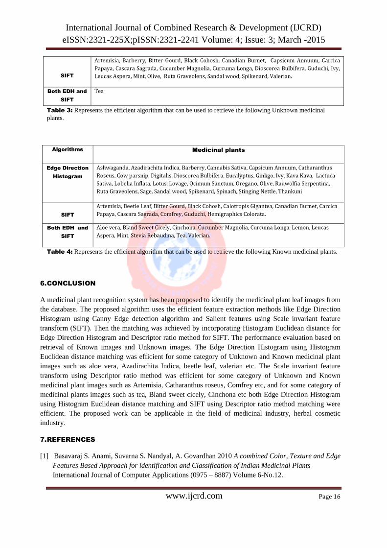
Table 3: Represents the efficient algorithm that can be used to retrieve the following Unknown medicinal
plants.
Algorithms Medicinal plants
Edge Direction
Histogram
Ashwaganda, Azadirachita Indica, Barberry, Cannabis Sativa, Capsicum Annuum, Catharanthus
Roseus, Cow parsnip, Digitalis, Dioscorea Bulbifera, Eucalyptus, Ginkgo, Ivy, Kava Kava, Lactuca
Sativa, Lobelia Inflata, Lotus, Lovage, Ocimum Sanctum, Oregano, Olive, Rauwolfia Serpentina,
Ruta Graveolens, Sage, Sandal wood, Spikenard, Spinach, Stinging Nettle, Thankuni
SIFT
Artemisia, Beetle Leaf, Bitter Gourd, Black Cohosh, Calotropis Gigantea, Canadian Burnet, Carcica
Papaya, Cascara Sagrada, Comfrey, Guduchi, Hemigraphics Colorata.
Both EDH and
SIFT
Aloe vera, Bland Sweet Cicely, Cinchona, Cucumber Magnolia, Curcuma Longa, Lemon, Leucas
Aspera, Mint, Stevia Rebaudina, Tea, Valerian.
Table 4: Represents the efficient algorithm that can be used to retrieve the following Known medicinal plants.
6. CONCLUSION
A medicinal plant recognition system has been proposed to identify the medicinal plant leaf images from
the database. The proposed algorithm uses the efficient feature extraction methods like Edge Direction
Histogram using Canny Edge detection algorithm and Salient features using Scale invariant feature
transform (SIFT). Then the matching was achieved by incorporating Histogram Euclidean distance for
Edge Direction Histogram and Descriptor ratio method for SIFT. The performance evaluation based on
retrieval of Known images and Unknown images. The Edge Direction Histogram using Histogram
Euclidean distance matching was efficient for some category of Unknown and Known medicinal plant
images such as aloe vera, Azadirachita Indica, beetle leaf, valerian etc. The Scale invariant feature
transform using Descriptor ratio method was efficient for some category of Unknown and Known
medicinal plant images such as Artemisia, Catharanthus roseus, Comfrey etc, and for some category of
medicinal plants images such as tea, Bland sweet cicely, Cinchona etc both Edge Direction Histogram
using Histogram Euclidean distance matching and SIFT using Descriptor ratio method matching were
efficient. The proposed work can be applicable in the field of medicinal industry, herbal cosmetic
industry.
7. REFERENCES
[1] Basavaraj S. Anami, Suvarna S. Nandyal, A. Govardhan 2010 A combined Color, Texture and Edge
Features Based Approach for identification and Classification of Indian Medicinal Plants
International Journal of Computer Applications (0975 – 8887) Volume 6-No.12.
SIFT
Artemisia, Barberry, Bitter Gourd, Black Cohosh, Canadian Burnet, Capsicum Annuum, Carcica
Papaya, Cascara Sagrada, Cucumber Magnolia, Curcuma Longa, Dioscorea Bulbifera, Guduchi, Ivy,
Leucas Aspera, Mint, Olive, Ruta Graveolens, Sandal wood, Spikenard, Valerian.
Both EDH and
SIFT
Tea
Page 12
International Journal of Combined Research & Development (IJCRD)
eISSN:2321-225X;pISSN:2321-2241 Volume: 4; Issue: 3; March -2015
www.ijcrd.com Page 17
[2] Basavaraj S. Anami, Suvarna S Nandyal, A. Govardhan 2012 Color and Edge Histogram based
Medicinal Plants’ Image Retrieval I.J. Image, Graphics and Signal Processing, 8, 24-35.
Basavaraj S. Anami, Suvarna Nandyal and A.Govardhan 2008 A Text based Approach to content
based information retrieval for Indian Medicinal plants International Journal of Physical Sciences,
ISSN 1992-1950, Vol.3 (11).
[3] Cinque.L, Ciocca.G, S. Levialdi, A. Pellicano, R. Schettini 2001 Color-based image Retrieval
using spatial-chromatic histograms Image and Vision Computing.
[4] Cholhong Im, Hirobumi Nishida, Kunii 1998 A hierarchical Method of Recognizing Plant Species
by Leaf Shape MVA’ 98 IAPR Workshops on Machine Vision Application.
[5] Dong Kwon Park, Yoon Seok Jeon, Chee Sun Won 2000 Efficient Use of Local Edge Histogram
Descriptor Proceedings of the 2000 ACM workshops on Multimedia Pages 51-54ACM.
[6] Faraj Alhwarin, Chao Wang, Danijela Ristic – Durrant 2008 Improved SIFT-Features matching for
object Recognition BCS International Academic Conference.
[7] Hanife Kebapci, Berrin Yanikoglu and Gozde Unal 2010 Plant Image Retrieval Using Color, Shape
and Texture the Computer Journal Advance Access published.
[8] Jyotismita Chaki and Ranjan Parekh 2012 Designing an Automated System for Plant Leaf
Recognition International Journal of Advances in Engineering and Technology, ISSN: 2231- 1963
Vol.2, Issue 1, pp.149-158.
[9] Ji-Xiang Du, De- Shuang Huang, Xiao- Feng Wang and Xiao GU 2006 Computer-aided Plant
species identification (CAPSI) based of leaf shape matching technique Transactions of the Institute
of Measurement and Control 28, 3, pp. 275-284.
[10] Kashif Iqbal, Michael O. Odetayo, Anne James 2012 Content-based image Retrieval Approach for
biometric security using color, texture and shape Features controlled by fuzzy heuristics Journal
of Computer and System Sciences 78, 1258-1277.
[11] Lowe D.G 2004 Distinctive image features from scale –invariant keypoints International Journal
of Computer vision 60(2), 91-110.
[12] Marius Tico, Taneli Haverinen, Pauli Kuosmanen 2000 A method of Color Histogram Creation
For Image Retrieval pp157-160.
[13] Padmavathi.G, Subhashini.P, Lavanya.P.K 2009 Performance evaluation of the various edge
Detectors and filters for the noise IR images ISSN: 1790 – 5117, ISBN: 978-960-474-135.
[14] Sathaya Bama. B, S.Mohana Valli, S.Raju, V.Abhai Kumar 2011 Content based Leaf Image
Retrieval (CBLIR) Using Shape, Color and Texture Features Indian Journal of Computer Science
and Engineering ISSN: 0976-5166, Vol.2.No2.
[15] Shitala Prasad, Krishna Mohan Kudri, and R.C. 2011 Relative Sub-Image based features for leaf
recognition using Support Vector Machine ICCCS’11.
[16] Shi Dong-cheng, XU LAN, Han Ling-yan 2007 Image retrieval using both Color and Texture
Features the Journal of China Universities of Posts and Telecommunications, Vol.14.
[17] Sandeep Kumar.E 2012 Leaf Color, Area and Edge features based Approach for Identification of
Indian Medicinal Plants Indian Journal of Computer Science and Engineering (IJCSE), ISSN:
0976-5166, Vol. 3 No.3.
[18] Yan Ke, Rahul Sukthankar 2003 PCA SIFT: A more distinctive representation for Local Image
Descriptor IRP-TR-03-15.