The Accuracy of Predicted Wages of the Non-Employed … Accuracy of Predicted Wages of the...

* Robert Breunig thanks the Australian Treasury forhospitality and support. We benefitted from commentsby Deborah Cobb-Clark, Jennifer Foster, Paul Frijters,Xiaodong Gong, Guyonne Kalb, Anthony King, PaulMiller and Marty Robinson. We are grateful to them.This paper uses confidentialised unit record data fromthe Household, Income and Labour Dynamics in Aus-tralia (HILDA) survey. The HILDA Project was initi-ated and is funded by the Commonwealth Departmentof Families, Community Services and IndigenousAffairs (FaCSIA) and is managed by the MelbourneInstitute of Applied Economic and Social Research(MIAESR). The findings and views reported in thispaper, however, are those of the authors and there is anon-countable set of people and organisations to whomthe findings and views should not be attributed includ-ing FaCSIA, MIAESR and the Australian Treasury.

JEL Classifications: C52, J22, J30, J64Correspondence: Robert Breunig, Economics Pro-

gram, Research School of Social Sciences, Building 9,Australian National University, Canberra, ACT 0200,

THE ECONOMIC RECORD, 2010

Australia. Email: [email protected]

The Accuracy of Predicted Wages of theNon-Employed and Implications for Policy

Simulations from Structural Labour Supply Models*

ROBERT BREUNIG

Economics Program, Research School of SocialSciences, Australian National University,

Canberra, Australia

1

� 2010 Australian TreasuryJournal compilation � 2010 The Economic Society of Austradoi: 10.1111/j.1475-4932.2009.00619.x

JOSEPH MERCANTE

Tax Analysis Division,Australian Treasury

We examine the accuracy of predicted wages for the non-employed. We argue that unemployment, marginal attachment,and not in the labour force are three distinct states. Using paneldata from Australia, we test the accuracy of predicted wages forthese three groups of non-employed using sample selection mod-els. Focusing on those individuals who subsequently enter employ-ment, we find that predictions which incorporate the estimatedsample selection correction perform poorly, particularly for themarginally attached and the not in the labour force. These resultshave important implications for policy simulations from structurallabour supply models.

l

I IntroductionLabour supply models are often used to pre-

dict responses of individuals to changes in gov-ernment tax and transfer systems. Of particularinterest in many developed countries is theeffect of such changes on individuals who arenot currently working. Many government pro-grammes around the world, such as earnedincome tax–credits and increased tax-freeincome thresholds for low earners, are specifi-cally designed to attract new workers into thework force and into employment.

An important aspect of the predictions fromthese labour supply models is the predictedwages which are generated for non-employedindividuals. These predicted wages directlydetermine the additional (predicted) utility thatnon-employed individuals will get from workingand therefore the predicted changes in employ-ment which will ensue from a policy change.For example, labour supply models will over-state (or understate) the employment benefits

ia

2 ECONOMIC RECORD MARCH

from tax cuts if wages of the non-workingare systematically over-predicted (or under-predicted).

Australian examples of the use of predictedwages in structural labour supply modellinginclude Duncan and Harris (2002), Kalb (2002),Kalb and Lee (2008) and Breunig et al. (2008).Predicted wages, corrected for sample selection,are used in a wide variety of other applicationsbeyond structural labour supply modelling. Forexample, Rammohan and Whelan (2005) generatepredicted wages for modelling the choice of child-care usage for working and non-working women.

The focus of this paper will be on two specificaspects of wage modelling for the non-working.First, we examine whether the unemployed, themarginally attached and those not in the labourforce should be treated identically or separatelyin modelling the probability of employment. Wepropose a new test for determining whether thenon-employed should be categorised as one,two or three groups. We find evidence that theunemployed, the marginally attached and the notin the labour force should be treated as threedistinct groups for modelling purposes.

In the second part of the paper, we examinethe wage predictions resulting from regressionswhich correct for selectivity bias using binomialand multinomial models of employment status.Specifically, we evaluate both conditional andunconditional wage predictions from these mod-els. Using a panel of data from Australia, wecompare predicted wages for the non-working tothe wages they actually receive when they sub-sequently enter the labour market.

Overall, we find that wage predictions fromwage equations which control for selection andwhich use information from the selection cor-rection perform poorly. Selection correctionterms are often poorly estimated and in smallsamples can be highly variable. For somegroups that we consider, this results in verypoor predictive performance. Including the esti-mated selection parameter in the wage equationleads to under-prediction of wages for the notin the labour force and marginally attachedgroups. For the unemployed, the results aremore mixed, but it is clear that using theconditional (on selection) predictor sometimesproduces very poor predictions. The main con-clusion from the paper is that researchers shouldexercise caution in the use of conditional pre-dictors for wages of the non-working, particu-larly in small samples.

Journal c

The paper is organised as follows. In SectionII, we discuss wage models which control forselection into employment. In Section III wediscuss our data. In Section IV, we discuss ourstrategy for testing whether the non-employedshould be pooled or considered separately. InSection V, we examine the wage predictionsfrom our models and compare them with rea-lised wages for those who transit from not work-ing to employment. We test which modelsgenerate the most accurate wage predictions. InSection VI we discuss our results and conclude.

II Wage Models with SelectionThe standard approach in the literature is that

proposed by Heckman (1979) whereby wages w�ifor all workers and non-workers depend upon avector of observable human capital characteris-tics, xi and some unobservable variables cap-tured by ui

lnðw�i Þ ¼ x0ibþ ui: ð1Þ

The actual wage, wi, is only observed if a latentvariable s�i > 0 where

s�i ¼ z0icþ vi ð2Þ

b and c are vectors of parameters and Equa-tion (2) provides a model for the probability ofemployment. This latter equation captures thebenefits of employment and therefore zi mustcontain all of the variables in xi. If we think ofthis model as arising in the context of the Heck-man (1974) reservation wage model, it shouldalso contain variables which affect the reserva-tion wage, which is (at least partially) determinedby the costs of employment. Importantly, ui andvi are assumed to be jointly, normally distributed.

The two-step empirical approach is to esti-mate c in Equation (2) and use those to estimate

lnðwiÞ ¼ x0ibþ qkðz0icÞ þ ui ð3Þ

on the sample with observed wages. The inclu-sion of the inverse Mills ratio, k, corrects forthe fact that E½vijs�i > 0� 6¼ 0. In a reservationwage model, q captures two effects. The firsteffect is that unobservable characteristics whichresult in a higher wage will also result in ahigher probability of employment. q will alsocapture the difference between the variance ofwage offers and the covariance between wageoffers and reservation wages. The first effectwill be positive. The second effect will be

� 2010 Australian Treasuryompilation � 2010 The Economic Society of Australia

2010 PREDICTED WAGES FOR THE NON-EMPLOYED 3

negative if the covariance between reservationwages and wage offers, which one would expectto be positive, is greater than the variance ofwage offers (see Ermisch & Wright, 1994).Empirically, it is not rare for the latter effect todominate and produce negative estimates of q.1

To predict wages from Equation (3), one hasseveral options. The unconditional predictor

E½lnðwiÞ� ¼ lnðwiÞ ¼ x0i b ð4Þ

gives the best estimate of the wage for the casewhere we do not know whether or not the indi-vidual is working. If we know that the individualis working, we can condition on this informationand use our model estimates to generate a condi-tional predicted wage for working individuals

E½lnðwiÞjs ¼ 1� ¼ lnðwei Þ ¼ x0i bþ q

/ðz0icÞUðz0icÞ

: ð5Þ

For those who are not employed, the conditionalprediction of wages will be

E½lnðwiÞjs ¼ 0� ¼ lnðwnei Þ ¼ x0i bþ q

�/ðz0icÞ1� Uðz0icÞ

:

ð6Þ

Note that in using Equations (5) and (6) we areconditioning on unobservable human capital char-acteristics and on the relationship between the dis-tributions of wage offers and reservation wages.2

If the model is correctly specified, the condi-tional predictor contains more information thanthe unconditional and Vella (1988) suggests itsuse in generating predicted wage gaps forblack–white or Man–Woman differences whichcondition on the work decision variables and theestimate of the parameter q. Use of the uncondi-tional predictor provides only an estimate of thewage gap experienced by those who work.Schaffner (1998) points out that using theunconditional predictor is only valid under veryrestrictive conditions. In particular, if there areunobserved traits that matter for one group andnot for the other, then wage gap estimates will

1 Dolton and Makepeace (1987) also discuss thedifficulty of interpreting sample selection effects andpoint out that it is erroneous to argue that participantshave lower earnings potential than non-participantswhen q is negative.

2 Hoffmann and Kassouf (2005) derive the marginaleffects in a log earnings equation using the condi-tional predictor.

� 2010 Australian TreasuryJournal compilation 2010 The Economic Society of Austral

be biased. Our focus will be on prediction forindividuals rather than groups and the keyassumption in using the conditional predictor isthat the distribution of unobservables, in partic-ular, the variances and covariances captured byq, are reasonably constant over time.

Puhani (2000) reviews some of the main cri-tiques of the Heckman selection approach. It hasbeen criticised on the grounds of not providingan improvement in predictive power (for work-er’s wages) relative to ordinary least squaresregression on the selected sample. It also suffersfrom potential collinearity problems when thevariables in z0i do not differ much from those inx0i. Lastly, the Heckman approach makes strongdistributional assumptions which, when violated,may lead to poor model performance as has beenvalidated in a number of Monte Carlo studies.These specification problems and the sensitivityof results to the strong model assumptions aregenerally found to be worse in small samples.3

In practice, one can estimate this model bypooling the unemployed, the marginally attachedand the not in the labour force to form the cate-gory of non-workers or one can exclude one ormore of these categories.4 Flinn and Heckman(1983) find that, for young men, the unemployedand the not in the labour force are distinct groupsand that the unemployment state facilitates jobsearch in line with standard search theory mod-els. Similar results are found by Tano (1991)for young people compared with older people,and Gonal (1992) for young women comparedwith young men. We will test whether theunemployed, the marginally attached and the notin the labour force are distinct groups and wewill also check whether the distinction makesany difference in accurately predicting wages.These tests are described below.

If non-employment can best be described as aset of distinct categories, there may be predic-tive gains in modelling them as such. In thatcase, several methods have been suggested.5

We begin with a multinomial model with J

3 Stolzenberg and Relles (1997) provide some intuitionabout specific mechanisms which can cause poor perfor-mance when using the Heckman selection approach.

4 Most Australian studies treat the unemployed andthe not in the labour force (including the marginallyattached) as a combined group of non-workers. Anexception is Ross (1986).

5 In this paper, we do not consider nested models,where a sequence of choices are made.

ia


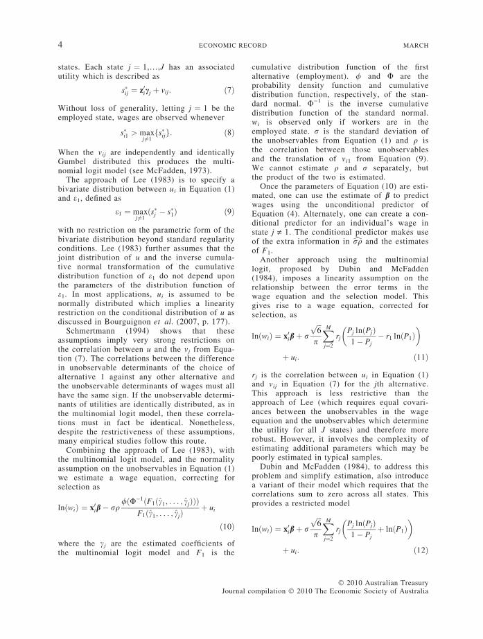
states. Each state j ¼ 1,…,J has an associatedutility which is described as

s�ij ¼ z0icj þ vij: ð7Þ

Without loss of generality, letting j ¼ 1 be theemployed state, wages are observed whenever

s�i1 > maxj6¼1fs�ijg: ð8Þ

When the vij are independently and identicallyGumbel distributed this produces the multi-nomial logit model (see McFadden, 1973).

The approach of Lee (1983) is to specify abivariate distribution between ui in Equation (1)and e1, defined as

e1 ¼ maxj6¼1ðs�j � s�1Þ ð9Þ

with no restriction on the parametric form of thebivariate distribution beyond standard regularityconditions. Lee (1983) further assumes that thejoint distribution of u and the inverse cumula-tive normal transformation of the cumulativedistribution function of e1 do not depend uponthe parameters of the distribution function ofe1. In most applications, ui is assumed to benormally distributed which implies a linearityrestriction on the conditional distribution of u asdiscussed in Bourguignon et al. (2007, p. 177).

Schmertmann (1994) shows that theseassumptions imply very strong restrictions onthe correlation between u and the vj from Equa-tion (7). The correlations between the differencein unobservable determinants of the choice ofalternative 1 against any other alternative andthe unobservable determinants of wages must allhave the same sign. If the unobservable determi-nants of utilities are identically distributed, as inthe multinomial logit model, then these correla-tions must in fact be identical. Nonetheless,despite the restrictiveness of these assumptions,many empirical studies follow this route.

Combining the approach of Lee (1983), withthe multinomial logit model, and the normalityassumption on the unobservables in Equation (1)we estimate a wage equation, correcting forselection as

lnðwiÞ ¼ x0ib� rq/ðU�1ðF1ðc1; . . . ; cjÞÞÞ

F1ðc1; . . . ; cjÞþ ui

ð10Þ

where the cj are the estimated coefficients ofthe multinomial logit model and F1 is the

Journal c

cumulative distribution function of the firstalternative (employment). / and U are theprobability density function and cumulativedistribution function, respectively, of the stan-dard normal. U)1 is the inverse cumulativedistribution function of the standard normal.wi is observed only if workers are in theemployed state. r is the standard deviation ofthe unobservables from Equation (1) and q isthe correlation between those unobservablesand the translation of vi1 from Equation (9).We cannot estimate q and r separately, butthe product of the two is estimated.

Once the parameters of Equation (10) are esti-mated, one can use the estimate of b to predictwages using the unconditional predictor ofEquation (4). Alternately, one can create a con-ditional predictor for an individual’s wage instate j „ 1. The conditional predictor makes useof the extra information in crq and the estimatesof F1.

Another approach using the multinomiallogit, proposed by Dubin and McFadden(1984), imposes a linearity assumption on therelationship between the error terms in thewage equation and the selection model. Thisgives rise to a wage equation, corrected forselection, as

lnðwiÞ ¼ x0ibþ r

ffiffiffi6p

p

XMj¼2

rjPj lnðPjÞ1� Pj

� r1 lnðP1Þ� �

þ ui: ð11Þ

rj is the correlation between ui in Equation (1)and vij in Equation (7) for the jth alternative.This approach is less restrictive than theapproach of Lee (which requires equal covari-ances between the unobservables in the wageequation and the unobservables which determinethe utility for all J states) and therefore morerobust. However, it involves the complexity ofestimating additional parameters which may bepoorly estimated in typical samples.

Dubin and McFadden (1984), to address thisproblem and simplify estimation, also introducea variant of their model which requires that thecorrelations sum to zero across all states. Thisprovides a restricted model

lnðwiÞ ¼ x0ibþ r

ffiffiffi6p

p

XMj¼2

rjPj lnðPjÞ1� Pj

þ lnðP1Þ� �

þ ui: ð12Þ



The linearity assumption proposed by Dubin andMcFadden (1984) restricts the class of allowabledistributions for u and imposes a specific formof linearity between u and Gumbel distributions(see Bourguignon et al., 2007, p. 179). Thisrestriction does not allow for u to be normallydistributed. Relative to Lee (1983), this providesa different set of assumptions which are not nec-essarily weaker or stronger.

Bourguignon et al. (2007) propose an alterna-tive restriction which allows normality of u.This restriction requires that the expected valueof u conditional on v1 to vj be a linear functionof the correlations between u and each v. Thishas the drawback of not providing a closed formsolution for the conditional expectations of thev1 to vj, but the numerical computation is notparticularly difficult.6

The wage, conditional on choosing to work, is

lnðwiÞ ¼ x0ibþr r�1mðP1Þ þXMj¼2

r�j mðPjÞPj

1�Pj

" #þui ð13Þ

where the m(P) are defined as

mðPjÞ ¼Z

U�1ðz� lnðPjÞÞ gðzÞ dz ð14Þ

and the g are the probability density function ofthe v which are assumed to be identically dis-tributed. r�j is the correlation between u andU)1(vj).

For the predicted wages of individuals whoare not working, we can again use an uncondi-tional or a conditional predictor.

We will use the four methods discussed aboveto predict wages for those who are not workingand compare them with the actual observedwages that those same individuals earn oncethey enter the labour force.7 We do this using

6 In implementing this method in Section V below,we use the STATA code of Bourguignon et al. (2007)available at the link provided in their paper.

7 Bourguignon et al. (2007) also discuss the semi-parametric estimator of Dahl (2002). We do not con-sider this estimator here because we are interested incomparing the parametric multinomial models withthe standard parametric Heckman model. An interest-ing project, beyond the scope of this paper, would beto compare wage predictions using the semi-paramet-ric variants of the Heckman model with those basedupon the model of Dahl.


panel data, which we describe in the nextsection.

III DataThe data are derived from the Household,

Income and Labour Dynamics in Australia Sur-vey (HILDA).8 The HILDA Survey is a nation-ally representative annual panel survey ofAustralian households and we use the first fivewaves from 2001 to 2005. There are around7500 households and around 13,000 respondingindividuals in each wave. After removingmulti-family households, same-sex couplehouseholds and couple households where part-ner information is unavailable, there are, inwave five, 3954 married women and men, 695lone parents, 1108 single women and 989single men.

We further restrict our sample to personsbetween 25 and 59 years of age, to excludethose facing decisions about full-time study orretirement. We drop the self-employed, workersin family businesses, full-time students andthe retired. Also dropped are those receivingdisability support pension, Department of Vet-eran’s Affairs disability pension or sicknessallowance. Finally, persons who report workingpositive hours but state a zero wage areremoved.9 For couples, we drop the observationif either member satisfies one of these condi-tions. The analysis sample contains 1492 mar-ried women and married men. In the finalsample of 484 lone parents, the majority (88 percent) are women. Also there are 315 singlewomen and 380 single men. The numbers arefairly similar for the earlier waves.

We discuss the definition of our key variables.Hours of labour supplied is defined as usualweekly hours of work in all jobs. The wage rateis defined as the person’s gross weekly salaryand wage income for all jobs divided by hours.For those not working, a wage of zero isassigned. Non-labour income is defined as thedifference between gross income and salary andwage income over the financial year. Welfareincome is income from pensions and benefits,

8 For more details, see Watson and Wooden(2002).

9 Less than 1 per cent of the working samplereported zero wage.

ia

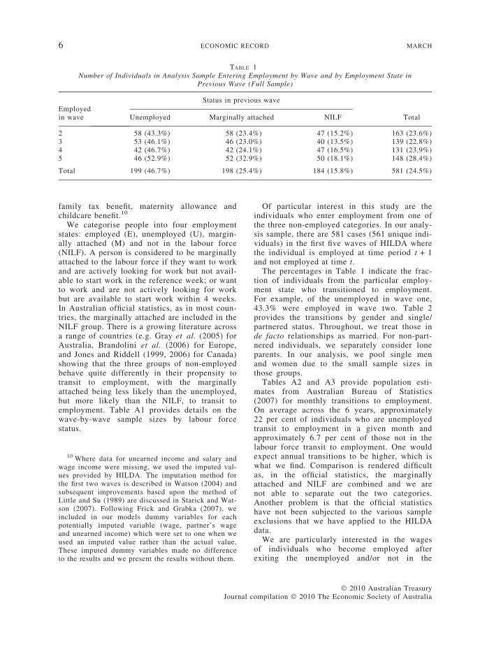
TABLE 1Number of Individuals in Analysis Sample Entering Employment by Wave and by Employment State in

Previous Wave (Full Sample)

Employedin wave

Status in previous wave

TotalUnemployed Marginally attached NILF

2 58 (43.3%) 58 (23.4%) 47 (15.2%) 163 (23.6%)3 53 (46.1%) 46 (23.0%) 40 (13.5%) 139 (22.8%)4 42 (46.7%) 42 (24.1%) 47 (16.5%) 131 (23.9%)5 46 (52.9%) 52 (32.9%) 50 (18.1%) 148 (28.4%)

Total 199 (46.7%) 198 (25.4%) 184 (15.8%) 581 (24.5%)


family tax benefit, maternity allowance andchildcare benefit.10

We categorise people into four employmentstates: employed (E), unemployed (U), margin-ally attached (M) and not in the labour force(NILF). A person is considered to be marginallyattached to the labour force if they want to workand are actively looking for work but not avail-able to start work in the reference week; or wantto work and are not actively looking for workbut are available to start work within 4 weeks.In Australian official statistics, as in most coun-tries, the marginally attached are included in theNILF group. There is a growing literature acrossa range of countries (e.g. Gray et al. (2005) forAustralia, Brandolini et al. (2006) for Europe,and Jones and Riddell (1999, 2006) for Canada)showing that the three groups of non-employedbehave quite differently in their propensity totransit to employment, with the marginallyattached being less likely than the unemployed,but more likely than the NILF, to transit toemployment. Table A1 provides details on thewave-by-wave sample sizes by labour forcestatus.

10 Where data for unearned income and salary andwage income were missing, we used the imputed val-ues provided by HILDA. The imputation method forthe first two waves is described in Watson (2004) andsubsequent improvements based upon the method ofLittle and Su (1989) are discussed in Starick and Wat-son (2007). Following Frick and Grabka (2007), weincluded in our models dummy variables for eachpotentially imputed variable (wage, partner’s wageand unearned income) which were set to one when weused an imputed value rather than the actual value.These imputed dummy variables made no differenceto the results and we present the results without them.

Journal c

Of particular interest in this study are theindividuals who enter employment from one ofthe three non-employed categories. In our analy-sis sample, there are 581 cases (561 unique indi-viduals) in the first five waves of HILDA wherethe individual is employed at time period t + 1and not employed at time t.

The percentages in Table 1 indicate the frac-tion of individuals from the particular employ-ment state who transitioned to employment.For example, of the unemployed in wave one,43.3% were employed in wave two. Table 2provides the transitions by gender and single/partnered status. Throughout, we treat those inde facto relationships as married. For non-part-nered individuals, we separately consider loneparents. In our analysis, we pool single menand women due to the small sample sizes inthose groups.

Tables A2 and A3 provide population esti-mates from Australian Bureau of Statistics(2007) for monthly transitions to employment.On average across the 6 years, approximately22 per cent of individuals who are unemployedtransit to employment in a given month andapproximately 6.7 per cent of those not in thelabour force transit to employment. One wouldexpect annual transitions to be higher, which iswhat we find. Comparison is rendered difficultas, in the official statistics, the marginallyattached and NILF are combined and we arenot able to separate out the two categories.Another problem is that the official statisticshave not been subjected to the various sampleexclusions that we have applied to the HILDAdata.

We are particularly interested in the wagesof individuals who become employed afterexiting the unemployed and/or not in the


TABLE 2Number of Individuals in Analysis Sample Entering Employment from Non-Employed State by Household Type

Subgroup

Status in previous wave

TotalUnemployed Marginally attached NILF

Married men 67 (60.9%) 21 (32.8%) 10 (19.2%) 98 (43.4%)Married women 49 (48.0%) 112 (26.7%) 145 (17.0%) 306 (22.3%)Single men 35 (39.8%) 12 (27.9%) 3 (17.7%) 50 (33.8%)Single women 17 (41.5%) 7 (31.8%) 5 (22.7%) 29 (34.1%)Lone parents 31 (36.5%) 46 (19.9%) 21 (9.3%) 98 (18.1%)

Total 199 (46.7%) 198 (25.4%) 184 (15.8%) 581 (24.5%)

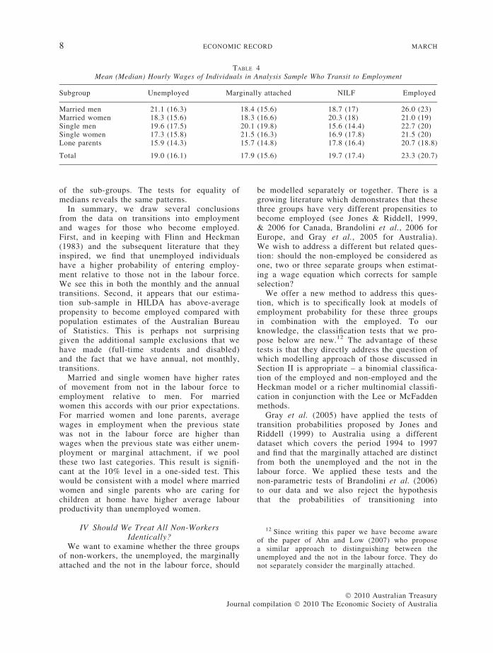
TABLE 3Mean (Median) Hourly Wages of Individuals in Analysis Sample Who Transit to Employment

From wave To wave Unemployed Marginally attached NILF Employed

1 2 19.6 (17.2) 17.2 (15.2) 18.6 (17) 21.8 (19.6)2 3 16.4 (15) 15.3 (14.6) 17.8 (15.6) 22.7 (20.2)3 4 20.3 (16.3) 18.9 (16.7) 21.8 (20) 23.6 (21)4 5 20.1 (17.4) 20.3 (16.7) 20.4 (18.3) 25.2 (22.2)

Total 19.0 (16.1) 17.9 (15.6) 19.7 (17.4) 23.3 (20.7)

11 If we conduct a non-parametric test of the equal-ity of the medians, we find similar results. The med-ian wages of the previously employed are significantlygreater than those of the previously not employed forall three sub-groups.


labour force categories. Predicted wages are ofinterest for those who are not working andtheir transition to employment will provide anopportunity to compare their wages with thoseof the continually employed and their actualwages when employed to predictions prior toemployment. Average hourly wages for oursample are given in Table 3 by wave andTable 4 by gender/partnered/lone parent split.The wages in Tables 3 and 4 are not correctedfor inflation.

We can test, using t-tests, whether meanwages in Table 3 are statistically differentdepending upon previous labour force status,without consideration of any individual charac-teristics. For those working, wages for the indi-viduals who were employed in the immediatelypreceding wave (the last column of Table 3) arestatistically larger (at the 10% level in all cases,at much lower levels for most cases) than wagesfor those who transition to employment fromany of the other labour force states. For themost part, wage differences between those whowere previously not in employment are not sta-tistically different from one another. The excep-tion is that for waves 2 and 3 and the pooleddata, we find that the employed who were previ-


ously NILF have statistically larger wages thanthe employed who were previously marginallyattached.11

Turning to the outcomes classified by sex andmarital status of Table 4, current mean wagesfor the previously employed are statisticallygreater than wages for the previously unem-ployed at the 6 per cent level or lower for allgroups. For married men, married women andlone parents, wages for the previously employedare statistically greater than wages for the previ-ously marginally attached. The sample sizes forsingle men and women are very small and it isdifficult to make any statistical statement aboutthese two groups of marginally attached. Wagesfor the previously employed are statisticallygreater than wages for the previously NILF forall groups except married women. Wages for thethree groups of previously non-employed are notstatistically different from one another for any

ia

TABLE 4Mean (Median) Hourly Wages of Individuals in Analysis Sample Who Transit to Employment

Subgroup Unemployed Marginally attached NILF Employed

Married men 21.1 (16.3) 18.4 (15.6) 18.7 (17) 26.0 (23)Married women 18.3 (15.6) 18.3 (16.6) 20.3 (18) 21.0 (19)Single men 19.6 (17.5) 20.1 (19.8) 15.6 (14.4) 22.7 (20)Single women 17.3 (15.8) 21.5 (16.3) 16.9 (17.8) 21.5 (20)Lone parents 15.9 (14.3) 15.7 (14.8) 17.8 (16.4) 20.7 (18.8)

Total 19.0 (16.1) 17.9 (15.6) 19.7 (17.4) 23.3 (20.7)

12 Since writing this paper we have become awareof the paper of Ahn and Low (2007) who proposea similar approach to distinguishing between theunemployed and the not in the labour force. They donot separately consider the marginally attached.


of the sub-groups. The tests for equality ofmedians reveals the same patterns.

In summary, we draw several conclusionsfrom the data on transitions into employmentand wages for those who become employed.First, and in keeping with Flinn and Heckman(1983) and the subsequent literature that theyinspired, we find that unemployed individualshave a higher probability of entering employ-ment relative to those not in the labour force.We see this in both the monthly and the annualtransitions. Second, it appears that our estima-tion sub-sample in HILDA has above-averagepropensity to become employed compared withpopulation estimates of the Australian Bureauof Statistics. This is perhaps not surprisinggiven the additional sample exclusions that wehave made (full-time students and disabled)and the fact that we have annual, not monthly,transitions.

Married and single women have higher ratesof movement from not in the labour force toemployment relative to men. For marriedwomen this accords with our prior expectations.For married women and lone parents, averagewages in employment when the previous statewas not in the labour force are higher thanwages when the previous state was either unem-ployment or marginal attachment, if we poolthese two last categories. This result is signifi-cant at the 10% level in a one-sided test. Thiswould be consistent with a model where marriedwomen and single parents who are caring forchildren at home have higher average labourproductivity than unemployed women.

IV Should We Treat All Non-WorkersIdentically?

We want to examine whether the three groupsof non-workers, the unemployed, the marginallyattached and the not in the labour force, should

Journal c

be modelled separately or together. There is agrowing literature which demonstrates that thesethree groups have very different propensities tobecome employed (see Jones & Riddell, 1999,& 2006 for Canada, Brandolini et al., 2006 forEurope, and Gray et al., 2005 for Australia).We wish to address a different but related ques-tion: should the non-employed be considered asone, two or three separate groups when estimat-ing a wage equation which corrects for sampleselection?

We offer a new method to address this ques-tion, which is to specifically look at models ofemployment probability for these three groupsin combination with the employed. To ourknowledge, the classification tests that we pro-pose below are new.12 The advantage of thesetests is that they directly address the question ofwhich modelling approach of those discussed inSection II is appropriate – a binomial classifica-tion of the employed and non-employed and theHeckman model or a richer multinomial classifi-cation in conjunction with the Lee or McFaddenmethods.

Gray et al. (2005) have applied the tests oftransition probabilities proposed by Jones andRiddell (1999) to Australia using a differentdataset which covers the period 1994 to 1997and find that the marginally attached are distinctfrom both the unemployed and the not in thelabour force. We applied these tests and thenon-parametric tests of Brandolini et al. (2006)to our data and we also reject the hypothesisthat the probabilities of transitioning into


FIGURE 1Probability of Employment at Subsequent Waves

Conditional on Initial Employment Status

13 Note that this is akin to the approach taken inHausman and McFadden (1984)

14 Another alternative would be the LR test of Cra-mer and Ridder (1991). In practice, this gives resultsvery similar to test T5 and we do not report thoseresults here.


employment are identical for any of the groupsof non-employed. We therefore confirm that theconclusions of Gray et al. (2005) are also foundfor the 2001–2006 period using the HILDAdata. Figure 1 shows the transitions to employ-ment by wave for all individuals in our analysissample who are non-employed at wave 1.

Turning to our proposed classification tests,we examine three different possibilities: that theunemployed (U) and the marginally attached(M) can be pooled; that the unemployed and thenot in the labour force (NILF) can be pooled,and that the marginally attached and the not inthe labour force can be pooled. If we find thattwo of these groups can be pooled, we can sub-sequently test whether that pooled group can bepooled with the third remaining category.

For each of the three pairings which we test,we propose five different classification tests. Weoutline these below using the test for poolingthe unemployed and the marginally attached asan example. Our testing approaches are basedupon estimation of binomial and multinomialchoice models. We estimate three probit models:

P1 Estimate probability of being employedusing E, U and M.

P2 Estimate probability of being employedusing E and M.

P3 Estimate probability of being employedusing E and U.

If the model which determines non-employ-ment is the same for the unemployed and themarginally attached, then P1, P2 and P3 shouldall (asymptotically) give similar answers. How-ever, P2 and P3 should be inefficient relative to


P1, as they only use a portion of the data. Thebasic principle underlying the Hausman (1978)test (comparison of two sets of coefficients, oneof which is consistently estimated under the nulland the other which is efficiently estimatedunder the null) therefore applies.13

Hence, our first two tests are:

T1 Hausman test comparing coefficients fromP1 to those of P2.

T2 Hausman test comparing coefficients fromP1 to those of P3.

We can also compare estimates from a multi-nomial choice model with those from a binarychoice model. For this comparison, we estimatetwo logistic models:

L1 Binary logit for probability of beingemployed using E, U and M.

L2 Multinomial logit allowing U and M to betwo distinct states.

Again, the Hausman principle applies and wehave two Hausman-type tests that can be pro-duced from these estimates:

T3 Hausman test comparing coefficients forunemployed from L1 and L2.

T4 Hausman test comparing coefficients formarginally attached from L1 and L2.

We can also use the multinomial logit esti-mates to conduct a Wald test to see if the coeffi-cients for the unemployed and marginallyattached states are equal.14

T5 F-test of equality of the coefficients for Uand M from L2.

The probit and logit models are estimatedusing age, age squared, a dummy for poorEnglish-speaking ability (self-assessed), a dummyvariable for being in New South Wales, adummy for living in a capital city, dummiesfor educational attainment, experience, experi-ence squared, partner’s wage, total unearnedhousehold income, number of resident childrenless than age 5, resident children aged 5–14,resident children aged >14, and non-residentchildren, a dummy variable if the individual

ia


owns their own home, a dummy if the individ-ual is a public tenant, and dummies forimputed household income and imputed part-ner’s wage.

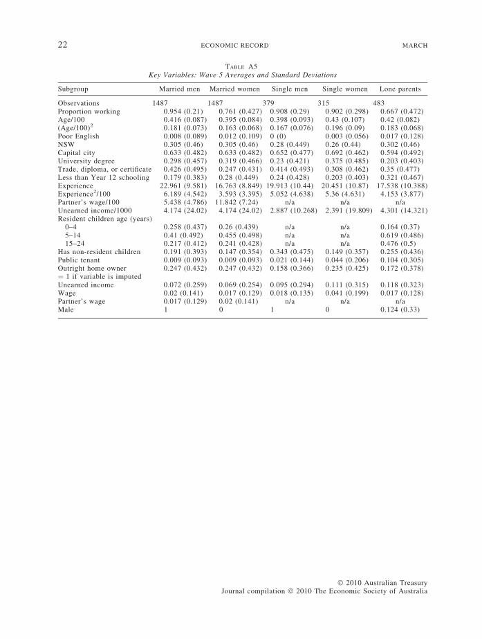
Table A5 contains a list of all the variablesused in these regressions and their means andstandard deviations from the fifth wave of thedata.15 We exclude any variables which do notvary for the sub-sample of interest (e.g. weexclude male from the sub-sample of marriedmen). We estimated all models with indicatorvariables if any of the wage or unearned incomedata were imputed (see footnote 10).

For each of our four sub-samples (marriedwomen, married men, lone parents and singles16)we conduct tests T1–T5 on each wave of data.We also conduct the tests on the data pooledacross all five waves. For the pooled models, weconduct the Hausman tests in two different ways.We use the standard variance matrix of para-meters uncorrected for the clustering which iscreated by the presence of multiple observationson the same individual in the pooled sample. Wealso conduct the Hausman tests using a variancematrix which is corrected for clustering using astandard outer-product correction. Neither arestrictly correct, as the former does not accountfor the clustering and the latter is not strictlytheoretically consistent with the Hausman test.Conclusions from the tests are consistent acrossboth methods, however.17

The test results for married women are sum-marised in Table 5.18 We focus on this groupbecause as they are a majority of the non-employed and a majority of those who transit toemployment. Second, they are a frequent focusof government policy. Given current highemployment in Australia, recent reforms to thetax and transfer system have been designed,at least in part, to induce married women who

15 Detailed descriptive statistics for other waves areavailable from the authors.

16 As noted previously, we pool single men andwomen due to small sample sizes.

17 We only report the results using the variance–covariance matrix which is not corrected for cluster-ing.

18 Results for lone parents, married men and singlesare available from the authors. Because of the smallsample sizes, we generally find no differences for theindividual waves. However, we find that the threestates are distinct in the pooled tests for all threegroups.

Journal c

are not in employment to enter the labourforce and to enter employment (see Centrelink,2008).

For married women, we find consistent evi-dence across all waves that the unemployed, thenot in the labour force and the marginallyattached are three distinct categories. Over 80per cent of the wave-by-wave tests show signifi-cant differences and we find significant differ-ences for all of the tests where we pool the dataacross waves.

In the last panel of Table 5, we combine themarginally attached and the NILF as is done inthe official statistics and test whether this com-bined group can be pooled with the unemployed.We can conclude from those tests that this com-bined group is also statistically significantly dif-ferent from the unemployed. As the wagepredictions which we discuss in Section V areoften estimated from models using ABS datawhich combine these two groups, we providethis test.

The conclusion we draw from these results isthat it is a mistake to pool the unemployed, themarginally attached and the not in the labourforce and to treat them identically in modellingthe probability of employment. This conclusionpoints the way to two possible modelling strate-gies for wage equations which correct for selec-tion into employment. The first is to model theemployed with each of the non-employed groupsseparately. This would suggest separate estima-tion of three Heckman selection models for thethree different groups. The problem with thisstrategy is that it is not clear which set of esti-mates one should use for understanding and pre-dicting wages for the employed. A secondmodelling strategy which follows from thesetests is to control for sample selection usingthe multinomial choice models discussed inSection II.19

In this paper, our main focus is on thosewho are not in employment. We examine in thenext section whether the results we have pre-sented have any implications for predictedwages for non-workers. For all three groups of

19 Instead of generating predicted wages from aselection model which are then plugged back into thelabour supply model, another alternative is to jointlymodel labour supply and the wage equation, with fourpossible labour market states, and simultaneously esti-mate wages and labour supply. For a three-stateexample, see Breunig et al. (2008)


TABLE 5Married Women: Can We Pool the Unemployed, the Marginally Attached and Not in the Labour Force?

Testa

Wave

Pooled1 2 3 4 5

Can we pool the not in the labour force and the unemployed?T1 0.00** 0.05* 0.21 0.01** 0.00** 0.00**T2 0.00** 0.00** 0.00** 0.00** 0.00** 0.00**T3 0.04** 0.05** 0.24 0.00* 0.00** 0.00**T4 0.00** 0.00** 0.00** 0.00** 0.00** 0.00**T5 0.00** 0.00** 0.00** 0.00** 0.00** 0.00**Can we pool the marginally attached and the unemployed?T1 0.01** 0.08** 0.66 0.00** 0.00** 0.00**T2 0.00** 0.00** 0.00** 0.00** 0.00** 0.00**T3 0.03** 0.10* 0.61 0.00* 0.00** 0.00**T4 0.00** 0.06* 0.19 0.01** 0.00** 0.00**T5 0.00** 0.05* 0.37 0.01** 0.00** 0.00**Can we pool the marginally attached and the not in the labour force?T1 0.00** 0.00** 0.00** 0.00** 0.00** 0.00**T2 0.00** 0.02** 0.00** 0.12 0.16 0.00**T3 0.00** 0.01** 0.00** 0.00** 0.03** 0.00**T4 0.00** 0.20 0.01** 0.17 0.02** 0.00**T5 0.00** 0.04** 0.00** 0.03** 0.02** 0.00**Can we pool the unemployed and a combined group of the not in the labour force and the marginally attached?T1 0.01** 0.07* 0.36 0.02** 0.00** 0.00**T2 0.00** 0.00** 0.00** 0.00** 0.00** 0.00**T3 0.12 0.15 0.41 0.15 0.09* 0.00**T4 0.00** 0.00** 0.01** 0.00** 0.00** 0.00**T5 0.00** 0.00** 0.03** 0.00** 0.00** 0.00**

Notes: Null hypothesis is that the two labour force states can be pooled. P-values for test of equality of labour force states arepresented. ** and * indicate significance at the 5 and 10 per cent levels, respectively. aThe five hypothesis tests, T1–T5, aredescribed in detail in the text.

20 Full results for lone parents, married men andsingles are available from the authors.


non-workers, we will examine the predictedwages from the different estimation strategies.We will then use the individuals who transitfrom non-work to employment to test which ofthese different estimation strategies provides themost accurate wage predictions for those non-workers who subsequently take up employment.

V The Accuracy of Predicted Wages UsingVarious Modelling Approaches

In the previous section, we concluded that theunemployed, the marginally attached and the notin the labour force appeared to be distinctgroups when modelling the probability ofemployment. In this section, we considerwhether these results have any relevance to theaccuracy of predicted wages for these threegroups.

Our basic approach will be as follows. Wewill estimate a model for wages in a particularcross-sectional wave, say wave t. We will then


use the estimated model to predict a wage, wit

for a non-employed individual. We then use anadjustment factor (at) to account for wage infla-tion between waves t and t + 1 to generate apredicted wage for individual i at time t + 1 as

wi;tþ1 ¼ witð1þ atÞ: ð15Þ

In the results presented below, we used theaverage increase in wages in our sample databetween wave t and t + 1 for the adjustment fac-tor. We also experimented with using the infla-tion rate of average weekly earnings from theAustralian Bureau of Statistics, but this did notaffect our conclusions.

We examine 11 separate models for predictingthe wages for married women.20 For eachmodel, we include all of the variables from

ia


Table A5. We exclude from the wage equationthe variables relating to unearned income, part-ner’s wage, resident and non-resident children,and home ownership status.

M1 Linear regression using only the em-ployed.

M2 Heckman selection model using wholesample and conditional predictor of Equa-tion (6).

M3 Heckman selection model using wholesample and unconditional predictor ofEquation (4).

M4 Heckman selection model using only non-working population of interest (unem-ployed, marginally attached or not in thelabour force) and conditional predictor ofEquation (6).

M5 Heckman selection model using only non-working population of interest and uncon-ditional predictor of Equation (4).21

M6 Lee selection model of Equation (10) andthe conditional predictor of wages.

M7 Lee selection model of Equation (10) andthe unconditional predictor of wages.

M8 The original multinomial model of Dubinand McFadden, Equation (12) and the con-ditional predictor of wages.

M9 The original multinomial model of Dubinand McFadden, Equation (12) and theunconditional predictor of wages.

M10 The restricted multinomial model of Bour-guignon, Fournier and Gurgand, Equation(13), and the conditional predictor ofwages.

M11 The restricted multinomial model of Bour-guignon, Fournier and Gurgand, Equation(13), and the unconditional predictor ofwages.

For each of these, we test whether the averagepredicted wage (wi;tþ1 above) is equal to theaverage realised wage for the three groupswhich transition into employment out of unem-ployment, marginal attachment or not in thelabour force.

21 Note that M4 and M5 would only be sensible ifthe other non-working groups could be theoreticallyexcluded from the model. M2 and M3 assume that thedistribution of unobservables is the same for all thenon-working groups. If the distribution of unobserv-ables is different for the non-working groups, but themodel applies to all of them, then the multinomialmodels are appropriate.

Journal c

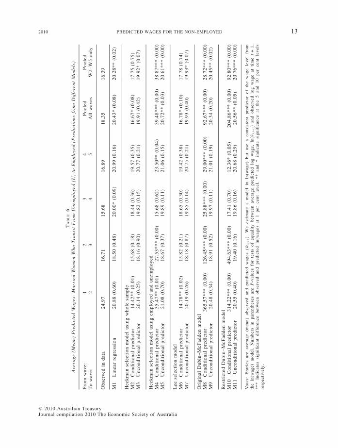
The results are summarised in Tables 6–8. Therows of the table present the average predictedwages for the group in question. The p-value ofthe test of equality between the predicted logwage and the actual, observed log wage for thosethat transition into employment are given justbelow the average predicted wages.22 We alsopool our predictions across all waves in column6. Column 7 presents the pooled results, droppingwave 1. For married women, we find oddly largewages for those in wave 2 who were unemployedin wave 1 (see Table 6). There appears to besome variability in responses to wage and incomequestions which settles down in subsequentwaves as respondents become more adept ataccurately completing the questionnaire. Wedropped the wave 1 to wave 2 changes to see ifour results were sensitive to any potential prob-lem. In our discussion, we will focus primarily onthe pooled results rather than the wave-by-waveresults. For the latter, sample sizes are sometimesfairly small and this introduces variability intothe results.

(i) Discussion of ResultsWe draw several conclusions from the results.

The first conclusion is that the unconditionalwage prediction from all of the models acrossall of the sub-groups is never statistically differ-ent from the wage prediction that one wouldmake based upon a linear regression model esti-mated only on the sub-population of workingindividuals.

The second unambiguous conclusion from theresults is that the conditional predictor whichuses the estimated sample selection parameter inthe prediction is highly variable. This is particu-larly true for the multinomial models where someof the conditional wage predictions are ludicrous.It is also true for the Heckman correction model.Looking at the pooled results in the row labelledM4 in Table 6, for example, we see that averagepredicted wages are nearly twice the average

22 For ease of reading, we present the wages inlevels. We have used a consistent predictor of thewage level based upon the estimates of the log wagemodel without imposing any parametric assumptions.As the model is estimated in log wage, we present theP-values of the test which compares predicted withactual log wage. We do this so that our tests are notinfluenced by the noise generated in estimating thescaling factor which we use to inflate exp[ln(wage)]to wage level.


TA

BL

E6

Ave

rag

e(M

ean

)P

red

icte

dW

ag

es:

Ma

rrie

dW

om

enW

ho

Tra

nsi

tF

rom

Un

emp

loye

d(U

)to

Em

plo

yed

(Pre

dic

tio

ns

fro

mD

iffe

ren

tM

od

els)

Fro

mw

av

e:

12

34

Po

ole

dP

oo

led

To

wav

e:

23

45

All

wav

es

W2

–W

5o

nly

Ob

serv

ed

ind

ata

24

.97

16

.71

15

.68

16

.89

18

.35

16

.39

M1

Lin

ear

reg

ress

ion

20

.88

(0.6

0)

18

.50

(0.4

8)

20

.00

*(0

.09

)2

0.9

9(0

.16

)2

0.4

3*

(0.0

8)

20

.28

**

(0.0

2)

Heck

man

sele

cti

on

mo

del

usi

ng

wh

ole

sam

ple

M2

Co

nd

itio

nal

pre

dic

tor

14

.42

**

(0.0

1)

15

.68

(0.1

8)

18

.44

(0.3

6)

19

.57

(0.3

5)

16

.67

*(0

.08

)1

7.7

5(0

.75

)M

3U

nco

nd

itio

nal

pre

dic

tor

20

.14

(0.2

5)

18

.16

(0.9

0)

19

.82

(0.1

5)

20

.77

(0.2

1)

19

.91

(0.4

2)

19

.92

*(0

.07

)

Heck

man

sele

cti

on

mo

del

usi

ng

em

plo

yed

an

du

nem

plo

yed

M4

Co

nd

itio

nal

pre

dic

tor

35

.47

**

(0.0

1)

27

.53

**

*(0

.00

)1

5.6

8(0

.62

)2

3.5

0*

*(0

.04

)3

9.4

8*

**

(0.0

0)

38

.87

**

*(0

.00

)M

5U

nco

nd

itio

nal

pre

dic

tor

21

.08

(0.7

0)

18

.67

(0.3

7)

19

.89

(0.1

1)

21

.06

(0.1

5)

20

.72

**

(0.0

3)

20

.61

**

*(0

.00

)

Lee

sele

cti

on

mo

del

M6

Co

nd

itio

nal

pre

dic

tor

14

.78

**

(0.0

2)

15

.82

(0.2

1)

18

.65

(0.3

0)

19

.42

(0.3

8)

16

.78

*(0

.10

)1

7.7

8(0

.74

)M

7U

nco

nd

itio

nal

pre

dic

tor

20

.19

(0.2

6)

18

.18

(0.8

7)

19

.85

(0.1

4)

20

.75

(0.2

1)

19

.93

(0.4

0)

19

.93

*(0

.07

)

Ori

gin

al

Du

bin

–M

cF

ad

den

mo

del

M8

Co

nd

itio

nal

pre

dic

tor

36

5.5

7*

**

(0.0

0)

12

6.4

5*

**

(0.0

0)

25

.88

**

*(0

.00

)2

9.0

0*

**

(0.0

0)

92

.67

**

*(0

.00

)2

8.7

2*

**

(0.0

0)

M9

Un

co

nd

itio

nal

pre

dic

tor

20

.48

(0.3

4)

18

.91

(0.5

2)

19

.97

(0.1

1)

21

.01

(0.1

9)

20

.34

(0.2

0)

20

.45

**

(0.0

2)

Rest

ricte

dD

ub

in–

McF

ad

den

mo

del

M1

0C

on

dit

ion

al

pre

dic

tor

31

4.2

2*

**

(0.0

0)

49

4.6

3*

**

(0.0

0)

17

.41

(0.7

0)

12

.36

*(0

.05

)2

04

.86

**

*(0

.00

)9

2.8

0*

**

(0.0

0)

M1

1U

nco

nd

itio

nal

pre

dic

tor

20

.55

(0.4

0)

19

.40

(0.1

6)

19

.86

(0.1

6)

20

.68

(0.2

9)

20

.56

**

(0.0

5)

20

.76

**

*(0

.00

)

No

tes:

En

trie

sare

av

era

ge

(mean

)o

bse

rved

an

dp

red

icte

dw

ag

es

(wi;

tþ1).

We

est

imate

am

od

el

inln

(wag

e)

bu

tu

sea

co

nsi

sten

tp

red

icto

ro

fth

ew

ag

ele

vel

fro

mth

eln

(wag

e)

mo

del.

Nu

mb

ers

inp

are

nth

ese

sare

P-v

alu

es

for

test

so

feq

uali

tyb

etw

een

av

era

ge

pre

dic

ted

log

wag

e,

lnðw

i;tþ

1Þ

an

do

bse

rved

log

wag

eat

tim

et

+1

.*

**

Ind

icate

ssi

gn

ifican

td

iffe

ren

ce

betw

een

ob

serv

ed

an

dp

red

icte

dln

(wag

e)

at

1p

er

cen

tle

vel.

**

an

d*

ind

icate

sig

nifi

can

ce

at

the

5an

d1

0p

er

cen

tle

vels

resp

ecti

vely

.


� 2010 Australian TreasuryJournal compilation 2010 The Economic Society of Australia

TA

BL

E7

Ave

rag

e(M

ean

)P

red

icte

dW

ag

es:

Ma

rrie

dW

om

enW

ho

Tra

nsi

tfr

om

No

tin

the

La

bo

ur

Fo

rce

(N)

toE

mp

loye

d(P

red

icti

on

sfr

om

Dif

fere

nt

Mo

del

s)

Fro

mw

av

e:

12

34

Po

ole

dP

oo

led

To

wav

e:

23

45

All

wav

es

W2

–W

5o

nly

Ob

serv

ed

ind

ata

18

.79

17

.89

22

.80

20

.77

20

.14

20

.63

M1

Lin

ear

reg

ress

ion

18

.46

(0.6

4)

18

.70

(0.3

5)

19

.64

(0.1

8)

21

.67

(0.2

4)

19

.80

(0.7

4)

20

.31

(0.5

6)

Heck

man

sele

cti

on

mo

del

usi

ng

wh

ole

sam

ple

M2

Co

nd

itio

nal

pre

dic

tor

14

.13

**

*(0

.00

)1

6.1

9(0

.15

)1

8.4

3*

*(0

.02

)2

0.4

3(0

.64

)1

6.7

9*

**

(0.0

0)

18

.16

**

(0.0

2)

M3

Un

co

nd

itio

nal

pre

dic

tor

17

.77

**

(0.0

4)

18

.37

(0.8

7)

19

.44

*(0

.09

)2

1.5

2(0

.33

)1

9.3

6(0

.20

)2

0.0

1(0

.77

)

Heck

man

sele

cti

on

mo

del

usi

ng

em

plo

yed

an

dn

ot

inth

ela

bo

ur

forc

eM

4C

on

dit

ion

al

pre

dic

tor

13

.57

**

*(0

.00

)1

5.4

0*

(0.0

5)

18

.42

**

(0.0

2)

19

.35

(0.9

0)

15

.88

**

*(0

.00

)1

7.1

6*

**

(0.0

0)

M5

Un

co

nd

itio

nal

pre

dic

tor

17

.96

(0.1

2)

18

.38

(0.8

0)

19

.50

(0.1

1)

21

.43

(0.3

7)

19

.38

(0.2

7)

19

.98

(0.7

5)

Lee

sele

cti

on

mo

del

M6

Co

nd

itio

nal

pre

dic

tor

14

.27

**

*(0

.00

)1

6.3

6(0

.21

)1

8.5

7*

*(0

.02

)2

0.2

9(0

.70

)1

6.8

7*

**

(0.0

0)

18

.18

**

(0.0

3)

M7

Un

co

nd

itio

nal

pre

dic

tor

17

.81

**

(0.0

5)

18

.39

(0.8

3)

19

.47

*(0

.09

)2

1.5

1(0

.34

)1

9.3

7(0

.22

)2

0.0

1(0

.77

)

Ori

gin

al

Du

bin

–M

cF

ad

den

mo

del

M8

Co

nd

itio

nal

pre

dic

tor

15

.96

**

*(0

.00

)8

.22

**

*(0

.00

)1

6.7

7*

**

(0.0

0)

10

.70

**

*(0

.00

)1

0.2

7*

**

(0.0

0)

8.7

4*

**

(0.0

0)

M9

Un

co

nd

itio

nal

pre

dic

tor

17

.85

*(0

.07

)1

8.7

3(0

.54

)1

9.5

4(0

.12

)2

1.4

9(0

.35

)1

9.6

2(0

.49

)2

0.3

1(0

.84

)

Rest

ricte

dD

ub

in–

McF

ad

den

mo

del

M1

0C

on

dit

ion

al

pre

dic

tor

16

.37

**

*(0

.00

)9

.35

**

*(0

.00

)1

7.5

4*

**

(0.0

0)

10

.57

**

*(0

.00

)1

1.9

6*

**

(0.0

0)

10

.40

**

*(0

.00

)M

11

Un

co

nd

itio

nal

pre

dic

tor

17

.92

(0.1

4)

19

.03

(0.1

0)

19

.46

*(0

.07

)2

1.3

1(0

.56

)1

9.8

0(0

.58

)2

0.5

6(0

.15

)

No

te:

See

no

tes

toT

ab

le6

.


� 2010 Australian TreasuryJournal compilation � 2010 The Economic Society of Australia

TA

BL

E8

Ave

rag

e(M

ean

)P

red

icte

dW

ag

es:

Ma

rrie

dW

om

enw

ho

Tra

nsi

tfr

om

Ma

rgin

all

yA

tta

ched

(M)

toE

mp

loye

d(P

red

icti

on

sfr

om

Dif

fere

nt

Mo

del

s)

Fro

mw

av

e:

12

34

Po

ole

dP

oo

led

To

wav

e:

23

45

All

wav

es

W2

–W

5o

nly

Ob

serv

ed

ind

ata

18

.71

16

.48

19

.58

18

.48

18

.40

18

.25

M1

Lin

ear

reg

ress

ion

18

.51

(0.8

2)

18

.82

*(0

.09

)1

8.5

7(0

.55

)2

1.5

9*

(0.0

9)

19

.52

(0.1

6)

20

.13

*(0

.06

)

Heck

man

sele

cti

on

mo

del

usi

ng

wh

ole

sam

ple

M2

Co

nd

itio

nal

pre

dic

tor

14

.10

**

*(0

.00

)1

6.2

1(0

.49

)1

7.3

0*

(0.0

8)

20

.30

(0.7

9)

16

.45

**

*(0

.00

)1

7.9

1(0

.23

)M

3U

nco

nd

itio

nal

pre

dic

tor

17

.68

*(0

.06

)1

8.4

6(0

.31

)1

8.3

8(0

.34

)2

1.4

9(0

.14

)1

9.0

8(0

.79

)1

9.8

5(0

.32

)

Heck

man

sele

cti

on

mo

del

usi

ng

em

plo

yed

an

dm

arg

inall

yatt

ach

ed

M4

Co

nd

itio

nal

pre

dic

tor

10

.90

**

*(0

.00

)1

4.8

5(0

.13

)1

5.8

4*

**

(0.0

1)

25

.54

**

*(0

.00

)1

4.1

9*

**

(0.0

0)

17

.56

(0.2

1)

M5

Un

co

nd

itio

nal

pre

dic

tor

17

.64

*(0

.08

)1

8.5

8(0

.19

)1

8.3

4(0

.35

)2

1.7

0*

(0.0

6)

19

.15

(0.8

3)

19

.99

(0.1

3)

Lee

sele

cti

on

mo

del

M6

Co

nd

itio

nal

pre

dic

tor

14

.28

**

*(0

.00

)1

6.3

5(0

.59

)1

7.4

5(0

.11

)2

0.1

6(0

.44

)1

6.5

3*

**

(0.0

0)

17

.92

(0.2

4)

M7

Un

co

nd

itio

nal

pre

dic

tor

17

.74

*(0

.07

)1

8.4

9(0

.28

)1

8.4

0(0

.36

)2

1.4

8(0

.14

)1

9.1

0(0

.83

)1

9.8

6(0

.31

)

Ori

gin

al

Du

bin

–M

cF

ad

den

mo

del

M8

Co

nd

itio

nal

pre

dic

tor

4.5

1*

**

(0.0

0)

45

.46

**

*(0

.00

)2

0.9

8(0

.36

)1

13

.75

**

*(0

.00

)3

0.1

9*

**

(0.0

0)

12

1.8

0*

**

(0.0

0)

M9

Un

co

nd

itio

nal

pre

dic

tor

17

.83

(0.1

1)

18

.88

(0.1

6)

18

.52

(0.4

5)

21

.73

(0.1

0)

19

.39

(0.6

7)

20

.24

(0.1

1)

Rest

ricte

dD

ub

in–

McF

ad

den

mo

del

M1

0C

on

dit

ion

al

pre

dic

tor

7.6

2*

**

(0.0

0)

53

.25

**

*(0

.00

)1

7.5

0*

(0.0

9)

91

.96

**

*(0

.00

)3

0.8

7*

**

(0.0

0)

99

.00

**

*(0

.00

)M

11

Un

co

nd

itio

nal

pre

dic

tor

17

.92

(0.2

0)

19

.23

**

(0.0

3)

18

.40

(0.2

9)

21

.62

(0.2

2)

19

.57

*(0

.09

)2

0.4

6*

**

(0.0

0)

No

te:

See

no

tes

toT

ab

le6

.


� 2010 Australian TreasuryJournal compilation 2010 The Economic Society of Australia

24 We are grateful to an anonymous referee whosuggested the additional tests and comparisons of thissection.


actual wage. This problem arises in part becausethe sample selection term is often estimated withvery low precision, at least in part due to smallsample sizes. The estimates of the sample selec-tion term are also unstable – switching betweennegative and positive for different waves of datausing the same population.23

The third conclusion is that there is no obvi-ous gain from using a multinomial model rela-tive to a simple Heckman correction model. Theconditional predictors from those models, as dis-cussed above, are highly unstable. The uncon-ditional predictors do not vary much from theunconditional predictor from the Heckmanmodel nor from the linear predictor from anOLS regression on the selected sample.

Our fourth conclusion is that a simple linearpredictor from a regression on the selected sam-ple or the unconditional predictor from the sam-ple selection model very often outperforms theconditional predictor which uses informationfrom the sample selection correction. This iscertainly the case for married women who movefrom not in the labour force to employment(M1, M3 and M5 in Table 7) and who movefrom marginal attachment to employment (M3and M5 in Table 8).

For married women who move from unemploy-ment to employment, the results are more mixed.The unconditional predictor works better (M3 ofTable 6) across all waves, but if we consideronly the last four waves, then the conditional pre-dictor works better. Given the extreme observa-tion for average wages for those who move fromunemployment in wave 1 to employment in wave2, we might prefer the conditional predictor forthis group. However, if we estimate the modelonly on the employed and unemployed (droppingthe not in the labour force and the marginallyattached), then the conditional predictor performsvery poorly. This is probably due to the smallsample size, but it is somewhat disturbing thatthe conditional predictor performs so differentlyin rows M2 and M4 of Table 6.

(ii) Comparing the Distributions of Predictedand Actual Wages

In Section V(i), we considered the differencesin the mean of actual and predicted wages.

23 For the Heckman selection models, Table A4provides a summary of the sign and significance ofthe estimated sample selection correction parameter.

Journal c

These comparisons may be sensitive to influen-tial observations. To check this, we testedwhether the medians of the predicted and actualwages were different for all of the models ofTables 6–8.24 If we consider the tests on thepooled data from the last two columns ofTables 6–8, the test of median equality and thatof mean equality agree (in terms of whether thedifferences are significant) for every single caseexcept for the unconditional predictor from theoriginal Dubin–McFadden model for unem-ployed, married women. We find that the meanwage from this model is not significantly differ-ent from the mean actual wage (P-value of 0.2,see row M9, column 6 of Table 6), whereas wefind that the medians are significantly different(P-value of 0.03). Given the over-whelming sim-ilarity between the results for medians and thosefor means, our main conclusions from SectionV(i) also appear to apply to the medians.25

We also conducted Kolmogorov–Smirnovtests on the equality of the distributions of pre-dicted and actual wages for the pooled models.For unemployed married women, the Kolmogo-rov–Smirnov test always agrees (in terms of sta-tistical significance/insignificance) with the testsof means shown in Table 6. For the not in thelabour force and the marginally attached, wealways reject that the distributions are identical,even when we find that the means of the distri-bution and medians of the distribution are notstatistically different.

To shed light on this latter result, Figures 2–4provide non-parametric density estimates ofthe actual ln(wage) and the predicted ln(wage)from the Heckman selection model estimatedusing the whole sample and pooling waves 2–5.Figure 2 corresponds to models M2 and M3 ofTable 6, Figure 3 corresponds to those modelsfrom Table 7, and Figure 4 corresponds tothose models from Table 8. Typically, predic-tions from wage models provide much moreconcentrated distributions than that of actualwages. We can clearly see this in all three fig-ures. It is this large peak and failure to capture

25 The vast majority of tests on the wave-by-wavecomparisons were also very similar for means andmedians. Versions of Tables 6–8 with median wagesand the results of the tests are available from theauthors.


FIGURE 2Actual and Predicted ln(wage) Distributions: Unemployed Married Women Who Become Employed

FIGURE 3Actual and Predicted ln(wage) Distributions: Not in the Labour Force Married Women Who Become Employed


the tails of the actual wage distribution that liesbehind the rejection of distribution equality wefind in the Kolmogorov–Smirnov test. The factthat we do not reject this equality for the unem-ployed is, we belief, primarily driven by thesmaller sample sizes for that sub-group. In bothFigures 3 and 4, we can see that the predictedwages which use the conditional predictor liewell to the left of the actual distribution ofwages and that the peak of the predicted andactual wage distributions are quite far apart.The peak of the distribution of wages using theunconditional predictor lies quite close to thepeak of the actual wage distribution; hence, ourfailure to reject the null that the average predic-tions are equal to the average wages.


Recall that for the unemployed, we preferredthe conditional predictor for this model on thebasis of the test of means and medians. How-ever, looking at Figure 2, the peak of theunconditional predictor actually appears closerto the peak of the actual wage distribution.The conditional predictor performs better onthe tests of means and medians because of therelatively thicker left-hand tail in the wagedistribution.

(iii) Selection Amongst the Newly EmployedOne might worry that those non-employed

individuals at period t who become employedat period t + 1 are not a random sample fromthe group of non-employed but are themselves

ia

FIGURE 4Actual and Predicted ln(wage) Distributions: Marginally Attached Married Women Who Become Employed


a selected sample with unobservable character-istics better than the average non-employedperson. In that case, our tests may be inter-preted as a test for the best predictor of wagesconditional on actually taking up employmentin subsequent periods. For some types of pol-icy simulations, this may be the relevant pre-dicted wage.

It is very difficult to get a good estimate ofthe unobservable characteristics for those whonever take up employment. For those who movefrom non-employment to employment, we canestimate the unobservable effects on wagesthrough the residual from the wage regression attime t + 1.26 If we take the residuals from awage regression estimated on the entire pooledsample of individuals who are employed andthen run a regression on a set of dummy vari-ables which indicate the previous employmentstatus (one wave prior), we find significantlynegative effects of having been either unem-ployed or marginally attached in the previousperiod.27 The unobservables for the previouslynot in the labour force are less than those of thepreviously employed, on average, but the differ-ence is not significant.

We find this result reassuring in regard to theamount of selection that might be present in oursample which moves from non-employment to

26 This will be independent of the estimate of thecorrelation between utility of employment and wagesestimated at time t.

27 We control for the clustering induced by thepooling of individuals over time.

Journal c

employment. We expect, a priori, that theunemployed and the marginally attached mighthave poorer unobservable labour market charac-teristics than the employed and this is in factwhat we find.

VI Discussion and ConclusionsIn a model of the probability of employment,

we find that the unemployed, the marginallyattached and the not in the labour force appearto be three distinct groups. This result is consis-tent across several different types of models anddifferent specification tests. The implication isthat these three groups should not be pooledtogether into one ‘non-employed’ group in ajoint model of wages and employment. Our con-clusion is based on specification tests of cross-sectional models which classify individuals intoone or another category. Looking at transitionsto employment, Gray et al. (2005) are led tosimilar conclusions for Australia using data cov-ering the period 1994–1997. Applying similartests to the transitions in our data, we come tothe same conclusion for the 2001–2005 period.

Building upon these results, we examine thewage predictions from a variety of modelsbeginning with a simple linear regression modelwhich has no controls for selection into employ-ment to more complicated models which allowfor multiple non-employment states. We findthat the linear predictor from a regression on theselected sample of workers almost always out-performs more complicated prediction strate-gies. Interestingly, this is the same conclusionthat is reached by Duan et al. (1983) for the



problem of predicting the dependent variable forthe selected sample. Our paper is the first toexamine the question of predictive power forthe non-selected sample.

The linear predictor does not always provideunbiased estimates of future wages, but it is lessprone to very large errors than conditional pre-diction based upon a sample selection model.This is primarily driven by the instability andimprecision of the estimated coefficient on thesample selection term in the second stage of thetwo-step modelling procedure. More compli-cated multinomial models appear to suffer fromthese problems to a greater degree than the bin-ary Heckman selection model.

For married women in the not in the labourforce and marginally attached categories, theselection model does not seem to provide infor-mation about the average effect of unobserv-ables on wages through the correlation with theselection equation. One possible explanation isthat the decision to move from one of thesenon-employed states to employment is accompa-nied by a change in the relationship between thereservation wage and the distribution of wageoffers as discussed in Section II above.

For unemployed, married women, however,there does seem to be information in the selec-tion model regarding unobservables, althoughthis result is somewhat sensitive to sample per-iod and size. The result is consistent with amodel that views unemployment as the state inwhich individuals better understand their reser-vation wage and truly are ready to take upemployment if the right offer comes along.

One important caveat to our results is thatthey are based upon fairly small sample sizes.When pooling across all five waves, we havearound 6000 married women but only approxi-mately 200 each in the categories of unem-ployed, marginally attached and not in thelabour force. These sample sizes are not out ofline with uses of selection models in the Austra-lian and overseas literature. Papers such as Dun-can and Harris (2002), Rammohan and Whelan(2005) and Breunig et al. (2008) use smallersample sizes in their selection models. Grogger(1998) uses a sample from the USA withapproximately 1100 individuals of whom 5.2 percent are non-employed. Beblo et al. (2003) usesample sizes ranging from 963 to 3235 in esti-mating selectivity-corrected gender wage gapsfor a variety of European countries. Kalb (2002)pools across four waves of the Survey of


Income and Housing Costs to get sample sizesthat are approximately 50 per cent larger thanthose used here. The data we use, HILDA, is theonly dataset in Australia which allows us toobserve subsequent employment and wage out-comes for the previously non-working. It wouldbe desirable to implement these tests on a muchlarger dataset, but this is currently not possiblein Australia. Despite the small samples, theresults are of interest as the HILDA data arewidely used for research in labour economics inAustralia.

All selection models start by making func-tional form assumptions about the relationshipbetween the unobservables in the equationswhich determine wages and participation. Wecan think of sample selection correction termsas then being estimated upon the residuals fromthese equations. Two problems arise. The first isthat, as in many models where we are estimatingfunctions of inferred quantities, large samplesizes are required for the (desirable) asymptoticproperties of the estimates to hold. Second, ourprocedure is dependent upon non-testable distri-butional assumptions, the failure of which maylead to biased or highly variable estimates.A priori, therefore, one might be suspiciousabout the use of the conditional predictor. Ourresults, although based on small samples, add anadditional cautionary note to the use of wageprediction augmented with information fromsample selection terms.

Some labour supply models use predictedwages in policy simulations to consider thelikely employment outcomes from changes to thetax and transfer system. Our paper provides twolessons for individuals who are estimating suchmodels using survey data. The first is that a one-size-fits-all approach to predicting wages forthose who are not working may be inappropriateas the unemployed, the marginally attached andthe not in the labour force appear to behave quitedifferently. The second conclusion is that predic-tion using a simple linear regression on theselected sample may be desirable on the groundsthat it is less subject to assumptions about distri-butional assumptions and small sample sizes.

REFERENCES

Ahn, S.C and Low, S. (2007), ‘A Parametric Test forthe Distinction Between Unemployed and Out ofthe Labour Force Statuses’, Seoul Journal of Eco-nomics, 20, 59–87.

ia


Australian Bureau of Statistics (2007). Labour Force,Australia. Detailed Electronic Delivery, March2007–Gross Flows (ST GM1), Australian Bureau ofStatistics. Datacube 6291.0.55.001.

Beblo, M., Beninger, D., Heinze, A. and Laisney, F.(2003), ‘Measuring Selectivity-Corrected GenderWage Gaps in the EU’, Centre for European Eco-nomic Research (ZEW) Discussion Paper No. 03-74,ZEW, Mannheim, Germany.

Bourguignon, F., Fournier, M. and Gurgand, M.(2007), ‘Selection Bias Corrections Based on theMultinomial Logit Model: Monte Carlo Compari-sons’, Journal of Economic Surveys, 21, 174–205.

Brandolini, A., Cipollone, P. and Viviano, E. (2006), ‘Doesthe ILO Definition Capture all Unemployment?’ Journalof the European Economic Association, 4, 153–79.

Breunig, R., Cobb-Clark, D. and Gong, X. (2008),‘Improving the Modeling of Couples’ Labour Sup-ply’, Economic Record, 84, 466–85.

Centrelink, (2008). Welfare to work. Centrelink Publi-cation, Commonwealth of Australia 2008. [Cited 17July 2009.] Available from http://www.centrelink.gov.au/internet/internet.nsf/services/welfare_work.htm.

Cramer, J. and Ridder, G. (1991), ‘Pooling States inthe Multinomial Logit’, Journal of Econometrics, 47,267–72.

Dahl, G.B. (2002), ‘Mobility and the Returns toEducation: Testing a Roy Model with MultipleMarkets’, Econometrica, 70, 2367–420.

Dolton, P. J. and Makepeace, G. H. (1987), ‘InterpretingSample Selection Effects’, Economics Letters, 24, 373–9.

Duan, N., Manning, W.G., Morris, C.N. and New-house, J.P. (1983), ‘A Comparison of AlternativeModels for the Demand for Medical Care’, Journalof Business and Economic Statistics, 1, 115–26.

Dubin, J.A. and McFadden, D.L. (1984), ‘An Economet-ric Analysis of Residential Electric Appliance Hold-ings and Consumption’, Econometrica, 52, 345–62.

Duncan, A. and Harris, M. (2002), ‘Simulating theBehavioural Effects of Welfare Reforms Among SoleParents in Australia’, Economc Record, 78, 264–76.

Ermisch, J.F. and Wright, R.E. (1994), ‘Interpretationof Negative Sample Selection Effects in Wage OfferEquations’, Applied Economics Letters, 1, 187–9.

Flinn, C.J. and Heckman, J.J. (1983), ‘Are Unemploy-ment and Out of the Labour Force BehaviorallyDistinct Labor Force States?’ Journal of LaborEconomics, 1, 28–42.

Frick, J.R. and Grabka, M.M. (2007), ‘Item Non-Response and Imputation of Labor Income in PanelSurveys from a Cross-National Comparison’, IZADiscussion Paper Number 3043, Institute for theStudy of Labor, Bonn, Germany.

Gonal, F. (1992), ‘New Evidence on Whether Unemploy-ment and Out of the Labor Force are Distinct States’,Journal of Human Resources, 27, 329–61.

Gray, M., Heath, A. and Hunter, B. (2005), ‘TheLabour Force Dynamics of the MarginallyAttached’, Australian Economic Papers, 44, 1–14.

Journal c

Grogger, J. (1998), ‘Market Wages and Youth Crime’,Journal of Labor Economics, 16, 756–91.

Hausman, J. (1978), ‘Specification Tests in Economet-rics’, Econometrica, 46, 1251–71.

Hausman, J.A. and McFadden, D. (1984), ‘Specifica-tion Tests for the Multinomial Logit Model’, Econo-metrica, 52, 1219–31.

Heckman, J.J. (1974), ‘Shadow Prices, Market Wagesand Labor Supply’, Econometrica, 42, 679–94.

Heckman, J.J. (1979), ‘Sample Selection Bias as aSpecification Error’, Econometrica, 47, 153–61.

Hoffmann, R. and Kassouf, A.L. (2005), ‘DerivingConditional and Unconditional Marginal Effects inLog Earnings Equations Estimated by Heckman’sProcedure’, Applied Economics, 37, 1303–11.

Jones, S.R.G. and Riddell, W.C. (1999), ‘The Mea-surement of Unemployment: an EmpiricalApproach’, Econometrica, 67, 147–61.

Jones, S.R.G. and Riddell, W.C. (2006), ‘Unemploy-ment and Nonemployment: Heterogeneties in LaborMarket States’, The Review of Economics and Statis-tics, 88, 314–23.

Kalb, G.R. (2002), ‘Estimation of Labour SupplyModels for Four Separate Groups in the AustralianPopulation’, Melbourne Institute Working PaperNo. 24/02. [Cited 5 January 2010.] Availablefrom: http://melbourneinstitute.com/wp/wp2002n24.pdf.

Kalb, G.R. and Lee, W.-S. (2008), ‘Childcare Use andParents Labour Supply in Australia’, Australian Eco-nomic Papers, 47, 272–95.

Lee, L.-F. (1983), ‘Generalized Econometric Modelswith Selectivity’, Econometrica, 51, 507–12.

Little, R.J.A. and Su, H.L. (1989), ‘Item Non-response in Panel Surveys’, in Kasprzyk D., Dun-can G.J., Kalton G. and Singh M.P. (eds), PanelSurveys. Wiley, New York; 400–25.

McFadden, D.L. (1973), ‘Conditional Logit Analysisof Qualitative Choice Behavior’, in Zarembka P.(ed.), Frontiers in Econometrics. Academic Press,New York; 105–42.

Puhani, P.A. (2000), ‘The Heckman Correction forSample Selection and its Critique’, Journal of Eco-nomic Surveys, 14, 53–68.

Rammohan, A. and Whelan, S. (2005), ‘Child Careand Female Employment Decisions’, AustralianJournal of Labour Economics, 8, 203–25.

Ross, R.T. (1986), ‘Analysis of the 1980 Sydney Sur-vey of Work Patterns of Married Women: FurtherResults’, Economic Record, 62, 325–37.

Schaffner, J.A. (1998), ‘Generating ConditionalExpectations from Models with Selectivity Bias:Comment’, Economics Letters, 58, 255–61.

Schmertmann, C.P. (1994), ‘Selectivity Bias Correc-tion Methods in Polychotomous Sample SelectionModels’, Journal of Econometrics, 60, 101–32.

Starick, R. and Watson, N. (2007), ‘Evaluation ofAlternative Income Imputation Methods for theHILDA Survey’, Technical Report. HILDA Project



Discussion Paper Series No. 1/07, Melbourne Insti-tute of Applied Economic and Social Research,Melbourne.

Stolzenberg, R.M. and Relles, D.A. (1997), ‘Tools forIntution about Sample Selection Bias and its Cor-rections’, American Sociological Review, 62, 494–507.

Tano, D.K. (1991), ‘Are Unemployment and Out ofthe Labour Force Behaviorally Distinct Labor ForceStates? New Evidence from the Gross ChangeData’, Economics Letters, 36, 113–7.

Vella, F. (1988), ‘Generating Conditional Expecta-tions from Models with Selectivity Bias’, EconomicsLetters, 28, 97–103.

Watson, N. (2004), ‘Income and Wealth Imputationfor Waves 1 and 2’, Technical Report. HILDA Pro-ject Technical Paper Series No. 3/04, MelbourneInstitute of Applied Economic and Social Research,Melbourne.

Watson, N. and Wooden, M. (2002), ‘The Household,Income and Labour Dynamics in Australia(HILDA) Survey: Wave 1 Survey Methodology’,Technical Report. HILDA Project Technical PaperSeries No. 1/02, Melbourne Institute of AppliedEconomic and Social Research, Melbourne.

Appendix

TABLE A1Sample Sizes by Wave, Employment Status, Gender

and Marital/Parental Status

� 2010 AuJournal com

stralipilat

Wave

1

an Treasion 2010

2

uryThe Ec

3

onomic

4

Society

5

Marriedmen

E
1802 1519 1484 1385 1418 U 77 47 43 22 30 M 24 31 24 24 20 N 35 48 23 24 19
Marriedwomen

E
1365 1140 1114 1075 1131 U 44 40 40 31 39 M 205 148 133 92 86 N 324 317 287 257 231
Singlemen

E
350 327 331 350 344 U 40 32 24 25 17 M 15 20 19 17 12 N 10 19 5 8 6
Singlewomen

E
288 284 289 275 284 U 17 16 13 10 10 M 9 6 9 10 10 N 11 23 7 8 11
Loneparents

E
305 300 315 303 322 U 37 26 24 27 33 M 99 80 67 67 63 N 70 76 74 75 65
Notes: E, employed; M, marginally attached; N, not in thelabour force; U, unemployed.

of Austral

TABLE A2Number (per cent) of Individuals Entering

Employment by Year and Employment State inPrevious Month

Year

ia

Fromunemployed

FromNILF
Total
2001
59.7 (19.7) 111.1 (7.0) 170.8 (9.0) 2002 61.4 (20.6) 98.1 (6.2) 159.6 (8.4) 2003 60.2 (21.1) 105.5 (6.6) 165.7 (8.8) 2004 56.8 (22.4) 106.5 (6.6) 163.3 (8.8) 2005 56.6 (24.0) 106.7 (6.9) 163.3 (9.2) 2006 57 (24.3) 112.8 (7.4) 169.8 (9.7)
Notes: Average of monthly transitions over calendar year,individuals’ ages 25–59.Source: Australian Bureau of Statistics (2007) Labour ForceSurvey.

TABLE A3Number (per cent) of Individuals Entering

Employment by Employment State in PreviousMonth

Subgroup
From
unemployed
FromNILF Total
Men
32.2 (22.3) 34 (8.2) 66.2 (11.8) Women 26.4 (21.4) 72.8 (6.3) 99.1 (7.7)
Total
58.6 (21.8) 106.8 (6.8) 165.4 (9.0)
Notes: Average of monthly transitions from 2001–2006 bysex, individuals’ ages 25–59.Source: Australian Bureau of Statistics (2007) Labour ForceSurvey.

Table A4Sign and Significance of Heckman Correction Term

in Models of Tables 6–8 (Married Women)

Wave
Pooled
1–5
Pooled
2–5
1 2 3 4 5
Whole sample(E, U, M, N)(Tables 6–8)

+***
+** + + + +*** +***
Reducedsample (E, U)(Table 6)

)
) + ) ) )*** )**
Reducedsample (E, M)(Table 7)

+***
+ + ) + +*** +
Reducedsample (E, N)(Table 8)

+***
+*** + + +** +*** +***
Notes: *** indicates significance at the 1 per cent level. **and * indicate significance at the 5 and 10 per cent levelsrespectively.


TABLE A5Key Variables: Wave 5 Averages and Standard Deviations

Subgroup
Married men M arried women
Journal com

Single men

pilation � 2010 T

Single women

� 2010 Auhe Economic So

Lone parents

Observations 1
487 1 487 3 79 3 15 4 83 Proportion working 0.954 (0.21) 0.761 (0.427) 0.908 (0.29) 0.902 (0.298) 0.667 (0.472) Age/100
2
0.416 (0.087) 0.395 (0.084) 0.398 (0.093) 0.43 (0.107) 0.42 (0.082)
(Age/100)
0.181 (0.073) 0.163 (0.068) 0.167 (0.076) 0.196 (0.09) 0.183 (0.068) Poor English 0.008 (0.089) 0.012 (0.109) 0 (0) 0.003 (0.056) 0.017 (0.128) NSW 0.305 (0.46) 0.305 (0.46) 0.28 (0.449) 0.26 (0.44) 0.302 (0.46) Capital city 0.633 (0.482) 0.633 (0.482) 0.652 (0.477) 0.692 (0.462) 0.594 (0.492) University degree 0.298 (0.457) 0.319 (0.466) 0.23 (0.421) 0.375 (0.485) 0.203 (0.403) Trade, diploma, or certificate 0.426 (0.495) 0.247 (0.431) 0.414 (0.493) 0.308 (0.462) 0.35 (0.477) Less than Year 12 schooling 0.179 (0.383) 0.28 (0.449) 0.24 (0.428) 0.203 (0.403) 0.321 (0.467) Experience 22.961 (9.581) 16.763 (8.849) 19.913 (10.44) 20.451 (10.87) 17.538 (10.388) Experience2/100 6.189 (4.542) 3.593 (3.395) 5.052 (4.638) 5.36 (4.631) 4.153 (3.877) Partner’s wage/100 5.438 (4.786) 11.842 (7.24) n/a n/a n/a Unearned income/1000 4.174 (24.02) 4.174 (24.02) 2.887 (10.268) 2.391 (19.809) 4.301 (14.321) Resident children age (years)
0–4
0.258 (0.437) 0.26 (0.439) n/a n/a 0.164 (0.37) 5–14 0.41 (0.492) 0.455 (0.498) n/a n/a 0.619 (0.486) 15–24 0.217 (0.412) 0.241 (0.428) n/a n/a 0.476 (0.5)
Has non-resident children
0.191 (0.393) 0.147 (0.354) 0.343 (0.475) 0.149 (0.357) 0.255 (0.436) Public tenant 0.009 (0.093) 0.009 (0.093) 0.021 (0.144) 0.044 (0.206) 0.104 (0.305) Outright home owner 0.247 (0.432) 0.247 (0.432) 0.158 (0.366) 0.235 (0.425) 0.172 (0.378) ¼ 1 if variable is imputed Unearned income 0.072 (0.259) 0.069 (0.254) 0.095 (0.294) 0.111 (0.315) 0.118 (0.323) Wage 0.02 (0.141) 0.017 (0.129) 0.018 (0.135) 0.041 (0.199) 0.017 (0.128) Partner’s wage 0.017 (0.129) 0.02 (0.141) n/a n/a n/a Male 1 0 1 0 0.124 (0.33)
stralian Treasuryciety of Australia

Date post:	19-Apr-2018
Category:	Documents
Upload:	doantruc
View:	221 times
Download:	3 times

The Accuracy of Predicted Wages of the Non-Employed … Accuracy of Predicted Wages of the...

Documents