The Adaptive Order FEM approach for vibro-acoustic ...€¦ · examples demonstrating its superior...

Inter-noise 2014 Page 1 of 10

The Adaptive Order FEM approach for vibro-acoustic simulations:

a report on a newly implemented technology with application

examples demonstrating its superior performance to conventional

FEM methods

Koen VANSANT1; Raphael HALLEZ

2

1,2 Siemens PLM Software, Belgium

ABSTRACT

This paper will discuss a newly implemented Adaptive Order Finite Element Method (FEM AO) and intents

to illustrate its superior performance to conventional FEM methods. The power of the new FEM AO

technology lies in the adaptive model size, which is accomplished by element order increase (p refinement)

and varies with frequency. This allows to work with an as lean as possible model at each frequency while at

the same time guaranteeing the requested accuracy.

Three different application examples are provided in which the computational performance of the new FEM

AO approach is compared with that of a conventional FEM method. Occasionally the comparison may also

include results from advanced Boundary Element Method (BEM) approaches, like the Fast Multipole BEM.

In the context of automotive applications, a first case reports on the simulation of acoustic transfer functions

for a full vehicle model up to 4 kHz to be used in a transfer path analysis model for prediction of pass-by

noise. A second application example concerns the noise radiating from a fan of an aero-engine, including the

effects of flow. A third example will illustrate the performance of a computation of the transmission loss for

an industrial muffler. The examples show that FEM AO delivers equally accurate results 2 to 20 times faster

compared to a conventional FEM and with a more efficient use of in-core memory.

Keywords: Finite Element Models, adaptive order, pass-by noise, aero-engine fan noise, industrial mufflers.

I-INCE Classification of Subjects Number(s): 75.3, 34, 13.1.5, 13.2.1

1. INTRODUCTION

For many devices, vehicles and other products we experience every day, the design and engineering

that led to the end product also contained an acoustical aspect. Indeed, the user’s experience and

perception of quality in a product is colored to some extent also by its vibro-acoustic performance.

Think about the sound inside a car when driving at high speed on the motorway or the vibrations when

driving over cobble stones, the noise an aircraft makes when flying over at low altitude, the noise of an

electric power generating gas turbine installation, etc… The numerous ISO standards and legislation

concerning noise emission alone already make clear that the vibro-acoustic aspects of a product are

important. It also needs no further explanation that companies even seek to go beyond being compliant

with legislation and actively target a superior acoustic performance with respect to their competitors to

obtain market share in the premium segment of their business.

Simulation of a product’s vibro-acoustic performance allows for many design iterations, which are

relatively inexpensive, and which support on their turn the luxury of needing only a single (or few)

relatively expensive production prototype(s). Assuming the simulation can indeed capture all relevant

physical phenomena and can provide results in a reasonable amount of time, only a single prototype

1 [email protected]

2 [email protected]

Page 2 of 10 Inter-noise 2014


needs to be tested, to confirm the predicted vibro-acoustic behavior and also to test of course all other

product performance aspects. This represents a great cost saving in the design process. But, as

indicated, the simulation models need to live up to the conditions of being representative for the

behavior of interest and they should have acceptable computational performance (1).

When it comes to simulating the vibro-acoustic performance of a design, the acoustic engineer has

a multitude of methodologies, processes and technologies at his disposal. For most of these techniques,

there are constraints with respect to the types of problems they allow to tackle. A classification might

be based for instance on time versus frequency domain and weakly versus strongly coupled (fluid

structure interaction) methods. In this paper, the authors will take a focus on harmonic (to be solved

preferably in the frequency domain) and weakly coupled acoustic problems. This doesn’t mean that the

approaches discussed further can only tackle this kind of problems. It only means that for this paper the

authors limit the applications to only these of weakly coupled harmonic kind. Note that ‘weakly

coupled’ means that the surface vibrations can exist but are not influenced by the acoustic pressure

field they generate. Another classification for acoustic simulation methods for harmonic problems is

based on the frequency range for which they can be used. Here we can make distinction for instance

between deterministic methods, like the Boundary Element Method (BEM) and Finite Element

Method (FEM), which capture the physics well at all frequencies but which lead to problematic model

sizes for high frequencies, and statistical and geometrical methods like Statistical Energy Analysis and

Ray Tracing methods respectively, which make some assumptions which are only valid at high

frequencies but only need a limited model size to provide plausible results (2)(3).

In many industrial applications, the geometrical size combined with the frequency range of

interest results in large deterministic simulation models and therefore lengthy computation times. In a

typical simulation process, one single model is used to cover the full frequency range of interest. This

to not lose too much time in creating different meshes for different frequency ranges. As the mesh

discretization is determined by the highest frequency of interest, the model is

over-sampled/over-discretized for the lower frequency ranges. Clearly any extension which can

alleviate the computational burden this model size brings or which can solve the obtained set of

equations in a faster manner is a step in the good direction. In this paper, the authors will elaborate on

a new development in the deterministic FEM method which allows extending its use to higher

frequencies and larger models. Indeed, such an improvement will allow for more design iterations

which translates in a better guarantee for a prototype product that meets the vibro-acoustical

performance requirements.

In the first section following this introduction, this new approach for the FEM, namely Adaptive

Order FEM (FEM AO), is discussed. This new solver has been implemented in LMS Virtual.Lab

Acoustics (4). As will be shown by three application examples in the section after, the FEM AO

outperforms the conventional FEM approach by a factor 2 to 20 for solving time. The three examples

cover three application domains: automotive, aerospace and mechanical industries in general.

2. THE ADAPTIVE ORDER FEM APPROACH

When applied to wave propagation problems, the conventional FEM method is known to suffer

from the so-called pollution effect, which is linked to cumulative dispersion errors. Since the

dispersion error increases with frequency, the mesh resolution required to obtain a reasonable accuracy

also increases with frequency and the use of the conventional low-order FEM is restricted in practice

to low frequencies. It is a well-known fact that high-order FEM or p-FEM, which resorts to

higher-order approximations, allows diminishing the resolution requirements and therefore the total

number of degrees of freedom to solve for a particular Helmholtz problem with a targeted accuracy.

Beriot et al. (5) have therefore tried quantifying the real benefits of a p-FEM approach on a full

three-dimensional Helmholtz problem. They found that the solving time required to compute their test

case (a square duct section with a plane wave propagating through it) with a given required accuracy

was diminishing with increasing element order. In other words, for the duct example at hand, fewer

higher order elements seemed to be more efficient compared to more lower order elements to predict

accurately the pressure field response. The total number of degrees of freedom (DOF) being less in the



higher order element case. A key idea of the high-order methods is that, due to the quality of its

approximation space, one element can contain much more information. At 10=f

eP for instance, a

single element can span up to two wavelengths.

Next to this superior efficiency of higher order elements, the even more important idea behind FEM

AO is to adjust the order f

eP of each element automatically prior to the computation depending on the

frequency f , the local speed of sound )(Mc , itself depending on the mean flow speed, and the

element dimension h , in order to guarantee a predefined accuracy. A simple rule of thumb would for

instance state (in case of no mean flow) that

8

8

0 λ

h

c

fhP

f

e => (1)

Essentially, higher orders are used at high frequencies and/or for large elements and low orders will

be employed at low frequencies and/or for small elements. Figure 1 illustrates some higher order shape

functions on a hexagonal element and provides a 2d example of frequency dependency of the element

orders. It makes clear that FEM AO allows for a much coarser discretization compared to conventional

FEM methods which use only first or second order shape functions.

Figure 1 – top: higher order shape functions,

bottom: frequency dependency of the element order

A performance comparison between FEM and FEM AO is carried out on the rectangular duct

Helmholtz problem for a full frequency sweep. A full frequency range of Hzf ]4000,100[= is

considered which corresponds to a non-dimensional Helmholtz number range of ]74,84.1[ , with

md 1= . A thin uniform linear FEM mesh, valid up to Hzf 3500max = using a 8λ<h resolution

rate, is generated as shown in Figure 2, top-left. A uniform coarse FEM AO mesh is also generated

with the same upper frequency limit (the upper maxf of a FEM AO mesh is reached when adaptive

rule indicates that 10>f

eP ). The FEM AO mesh is obviously much coarser and the number of nodes

and elements is two orders of magnitude lower than for the FEM mesh. To test the ability of the FEM

AO solver to cope with strong local mesh refinements, two other meshes were generated as displayed

in Figure 2. These have the same upper frequency limit of Hzf 3500max = , but have one or all faces

with refined elements, to represent the situation in which such a refinement is required to accurately

capture the geometry of a more complex structure (a car for instance). In all models, the

Automatically Matched Layer (AML) (6) approach was used to mimic the fact that the duct only has 4

hard walls and continues infinitely.



Figure 2 – FEM cube mesh (upper left), FEM AO

cube mesh #1 (upper right), mesh #2 (lower left) and

mesh #3 (lower right). All meshes are valid up to

3500 Hz

Figure 3 - Comparison of the accuracy obtained

with FEM and FEM AO models as a function

of frequency

The numerical results obtained for the four meshes are compared with the analytical solution and

the numerical error is displayed along the full frequency range in Figure 2. The FEM model is very

accurate at low frequency, which is expected because the problem is clearly over resolved in this range.

However the FEM model yields larger errors at higher frequencies. On the other hand, the error for

FEM AO is stable and remains close to %1 on the full frequency range. This result is quite

remarkable for the FEM AO meshes #2 and #3 and indicates that the FEM AO solver can guarantee a

close to constant accuracy even in the case of highly non-uniform meshes.

In Figure 4, the time required per frequency is displayed for the four models. As expected, it is

constant for the FEM, while it increases with frequency for the FEM AO models. The local mesh

refinements in mesh #2 and mesh #3 come at the price of significant losses of performance but these

models remain much faster than the FEM. The total memory gains are also significant, as illustrated by

Figure 5. Again the FEM memory requirements are constant, whereas they start really low and

gradually increase with frequency for the FEM AO models. It should be noted that this memory

statement includes also the matrix storage, which in the case of FEM AO can become non negligible

(the high-order matrices are typically more densely populated).

Figure 4 - Comparison of the timings obtained

with linear FEM and the different FEM AO

models as a function of frequency.

Figure 5 - Comparison of the memory

required with linear FEM and the different

FEM AO models as a function of frequency.



3. APPLICATION CASES DEMONSTRATING FEM AO PERFORMANCE

In all examples shown, there is a need for a non-reflective FEM boundary, to mimic the fact that the

fluid surrounding the object at hand is surrounded by an unbounded fluid, or (in case of the muffler

examples shown in that section) to represent an endlessly continuing duct. This anechoic behavior is

inserted into the FEM or FEM AO model by means of the Automatically Matched Layer technology

(AML) (6). This AML allows the FEM models to remain relatively small and therefore fast to solve.

Next to that also a good solver for the acoustic matrix equations is needed. All models were solved

using a direct MUMPS solver (7).

3.1 Prediction of Acoustic Transfer Functions for Pass-By Noise (PBN)

Recently the debate on pass by noise has been revived as regulations are targeting lower sound

pressure levels for future cars (70 dBA Overall Level). Figure 6 schematically represents the setup for

an in-room pass by noise measurement. The car is put on a chassis-dyno and a speed as prescribed in

ISO 362 (for instance 50 km/h) is applied. The in-room tests have the benefit of providing perfect

‘weather conditions’ and guaranteeing repeatability. A set of near field FRFs measured between

indicator microphones ju and sources iQ (typically monopoles: 2 per tire, one for exhaust, intake, 6

monopoles for the engine) is measured as well as the far field target FRFs between target microphones

at positions ky and the same sources. The latter represent an equivalent set of FRFs as the one that

would be obtained by using only one microphone y left and one right and moving the car. Using TPA

techniques, explained in a more detailed manner in for instance (3), the PBN can then be constructed

based on an identification step of the noise sources followed by a computation of their noise

contributions and total pressure result and this for varying relative positions of the sources with respect

to the receiver.

Figure 6 - Pass by noise in-room test setup:

source-transfer-receiver concept

Figure 7 - FEM AO Model for computing

PBN FRFs

Using simulation models we can evaluate different sound proofing layouts, for instance in the

engine bay or around the muffler area, and see how these affect the noise transfer functions from the

vehicle sources to the receiver microphones 7.5 meters away from the car. As the results should

typically be available up to 4 or 5 kHz, the challenge in such simulations is the model size. Figure 7

shows the setup of a PBN model for a Chrysler Neon with field points (reciproque FRF computation)

for engine, tyres and exhaust and with sources (19 on each side) at 7.5 m from the centreline of the

vehicle ranging from -6 m (behind) to +12 m with respect to the back of the car. A FEM AO model was

used with larger elements to fill in void spaces and smaller elements to capture the scattering

boundaries of the full vehicle.

Table 1 reports the details on model sizes, in terms of mesh nodes and number of DOFs, for the

FEM AO and normal FEM models. Both use AML and a symmetry plane to model the floor. Note how

FEM AO needs less DOFs for the same accuracy when reaching higher frequencies. Three frequency



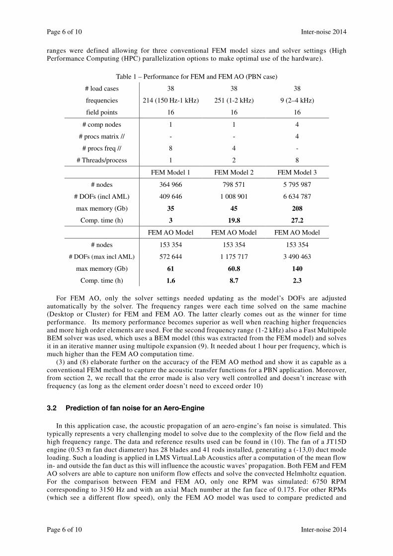
ranges were defined allowing for three conventional FEM model sizes and solver settings (High

Performance Computing (HPC) parallelization options to make optimal use of the hardware).

Table 1 – Performance for FEM and FEM AO (PBN case)

# load cases 38 38 38

frequencies 214 (150 Hz-1 kHz) 251 (1-2 kHz) 9 (2–4 kHz)

field points 16 16 16

# comp nodes 1 1 4

# procs matrix // - - 4

# procs freq // 8 4 -

# Threads/process 1 2 8

FEM Model 1 FEM Model 2 FEM Model 3

# nodes 364 966 798 571 5 795 987

# DOFs (incl AML) 409 646 1 008 901 6 634 787

max memory (Gb) 35 45 208

Comp. time (h) 3 19.8 27.2

FEM AO Model FEM AO Model FEM AO Model

# nodes 153 354 153 354 153 354

# DOFs (max incl AML) 572 644 1 175 717 3 490 463

max memory (Gb) 61 60.8 140

Comp. time (h) 1.6 8.7 2.3

For FEM AO, only the solver settings needed updating as the model’s DOFs are adjusted

automatically by the solver. The frequency ranges were each time solved on the same machine

(Desktop or Cluster) for FEM and FEM AO. The latter clearly comes out as the winner for time

performance. Its memory performance becomes superior as well when reaching higher frequencies

and more high order elements are used. For the second frequency range (1-2 kHz) also a Fast Multipole

BEM solver was used, which uses a BEM model (this was extracted from the FEM model) and solves

it in an iterative manner using multipole expansion (9). It needed about 1 hour per frequency, which is

much higher than the FEM AO computation time.

(3) and (8) elaborate further on the accuracy of the FEM AO method and show it as capable as a

conventional FEM method to capture the acoustic transfer functions for a PBN application. Moreover,

from section 2, we recall that the error made is also very well controlled and doesn’t increase with

frequency (as long as the element order doesn’t need to exceed order 10)

3.2 Prediction of fan noise for an Aero-Engine

In this application case, the acoustic propagation of an aero-engine’s fan noise is simulated. This

typically represents a very challenging model to solve due to the complexity of the flow field and the

high frequency range. The data and reference results used can be found in (10). The fan of a JT15D

engine (0.53 m fan duct diameter) has 28 blades and 41 rods installed, generating a (-13,0) duct mode

loading. Such a loading is applied in LMS Virtual.Lab Acoustics after a computation of the mean flow

in- and outside the fan duct as this will influence the acoustic waves’ propagation. Both FEM and FEM

AO solvers are able to capture non uniform flow effects and solve the convected Helmholtz equation.

For the comparison between FEM and FEM AO, only one RPM was simulated: 6750 RPM

corresponding to 3150 Hz and with an axial Mach number at the fan face of 0.175. For other RPMs

(which see a different flow speed), only the FEM AO model was used to compare predicted and



measured results. Figure 8 shows how the FEM models were constructed for this fan noise application.

The directivity of this axisymmetric model was examined from 25 deg from the centerline till 120 deg

from the centerline (i.e. behind the angle that can be seen from the center of the duct). The directivity

was obtained by computing the SPL at 25 m distance from the fan.

Figure 8 – Aero-engine acoustic model for simulation of fan noise

Figure 9 illustrates the directivity results and indicates a good match between FEM, FEM AO and

measurement for the 6750 RPM case. Also at 8450 RPM the FEM AO results correspond quite well

with experimental results.

Figure 9 – Comparison of FEM, FEM AO and experimental results for

6750 RPM (3150 Hz) (left) and 8450 RPM (3943 Hz) (right)

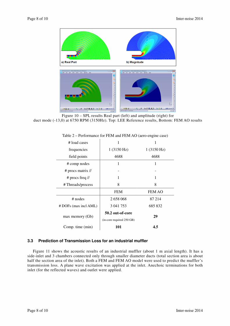
Figure 10 provides a plot of the acoustic SPL in the vicinity of the fan and shows a good match with

the reference method based on LEE (Linearized Euler Equations).

It should be noted that the maximum frequency for which the finite elements are valid depends on

the frequency rule (eg 8 els per wavelength) and on the local Mach number of the flow. As it is difficult

to only locally refine the mesh in a conventional FEM context based on the flow results, an acoustic

engineer will often refine the full mesh in order to make sure the majority of the elements are valid up

for the frequency range of interest. This means however that many elements are needlessly too small

and the model size therefore often too large. In the FEM AO approach, the solver increases the order

for each element individually, based on the frequency of the analysis and the element’s mean flow

speed. FEM AO therefore again ensures a more optimal model size, on element and full model level.

The consequences of the mesh requirements can be seen clearly also in Table 2, which lists the

performance of both FEM and FEM AO approach for the 6750 RPM case. The FEM AO model needed

only 700 000 DOFs for this frequency and therefore can deliver the results in 5 minutes with less than

30 GB of in-core memory, whilst the conventional FEM model needed to solve out-of-core and took

more than 20 times longer.



Figure 10 – SPL results Real part (left) and amplitude (right) for

duct mode (-13,0) at 6750 RPM (3150Hz). Top: LEE Reference results, Bottom: FEM AO results

Table 2 – Performance for FEM and FEM AO (aero-engine case)

# load cases 1 1

frequencies 1 (3150 Hz) 1 (3150 Hz)

field points 4688 4688

# comp nodes 1 1

# procs matrix // - -

# procs freq // 1 1

# Threads/process 8 8

FEM FEM AO

# nodes 2 658 068 87 214

# DOFs (max incl AML) 3 041 753 685 832

max memory (Gb) 50.2 out-of-core

(in-core required 250 GB) 29

Comp. time (min) 101 4.5

3.3 Prediction of Transmission Loss for an industrial muffler

Figure 11 shows the acoustic results of an industrial muffler (about 1 m axial length). It has a

side-inlet and 3 chambers connected only through smaller diameter ducts (total section area is about

half the section area of the inlet). Both a FEM and FEM AO model were used to predict the muffler’s

transmission loss. A plane wave excitation was applied at the inlet. Anechoic terminations for both

inlet (for the reflected waves) and outlet were applied.



Figure 11 – Muffler design and acoustic response for plane wave

excitation at 3 (left) and 5 kHz (right)

Figure 12 – Predicted muffler transmission loss using FEM and FEM AO

A good match between FEM and FEM AO results for the muffler’s transmission loss can be seen in

figure 12. Table 3 provides the performance numbers. Again, FEM AO is a lot faster compared to FEM.

This is mainly due to the lean model size it used in the lower frequency range. At the highest frequency,

still only about 200 000 DOFs are required, which is about half the amount needed by the conventional

FEM. This is due to the efficiency of the basis of shape functions used as explained earlier in this paper.

For the total simulation, FEM AO needed about half the memory used by FEM and it was more than 6

times faster.

Table 3 – Performance for FEM and FEM AO (industrial muffler case)

# load cases 1 1

frequencies 140 (50 Hz-7 kHz) 140 (50 Hz-7 kHz)

field points 2 121 2 121

# comp nodes 1 1

# procs matrix // - -

# procs freq // 4 4

# Threads/process 2 2



FEM FEM AO

# nodes 406 352 21 594

# DOFs (max incl AML) 406 352 205 301

max memory (Gb) 14.2 7.3

Comp. time (min) 30.8 4.8

4. CONCLUSIONS

In this paper the main concepts and characteristics of a new FEM solver with adaptive order, FEM

AO, were explained based on an academic duct acoustics problem with plane wave propagation. The

new technique was afterwards compared mainly to a conventional FEM approach and this for three

application cases: computation of acoustic transfer functions for a full vehicle model up to 4 kHz in

support of pass-by noise predictions, the simulation of aero-engine fan noise and prediction of

transmission loss for an industrial muffler. In all of these cases, FEM AO’s superiority in

computational performance over that of a conventional FEM method was shown. Factors between 2

and 20 times faster are typically observed. For the automotive case FEM AO also outperformed a Fast

Multipole BEM approach. Also with respect to memory, FEM AO often requires a smaller amount

compared to conventional FEM, as its more efficient basis of shape functions allows to use a smaller

amount of DOFs (compared to FEM) for the same accuracy. The latter is mostly valid for the higher

frequencies. Whereas the emphasis of this paper was to demonstrate the high speed and relatively low

memory consumption of FEM AO, its accuracy was also shown by comparison with either the

equivalent FEM model or with experimental results. This paper demonstrates therefore the power of

the new FEM AO approach for simulating deterministic acoustic problems.

REFERENCES

1. Van der Auweraer H, Leuridan J, The new paradigm of testing in today’s product development process,

Proceedings of the ISMA2004 Conference, 1151-1170, 2004

2. Vansant K, Hallez R, Bériot H, Tournour M et al., Simulating acoustic engine performance over a broad

frequency range, SAE Technical Paper 2011-26-0019, 2011, doi:10.4271/2011-26-019

3. Vansant K, Latest developments in solving large simulation models in view of pass-by noise,

AIA-DAGA, 2013

4. Virtual.Lab 13.1 User manual

5. Beriot H, Prinn A, Gabard G , On the performance of high-order FEM for solving large scale industrial

acoustic problems, ICSV 20, 2013

6. Bériot H, Tournour M, On the locally-conformal perfectly matched layer implementation for Helmholtz

equation, NOVEM Noise and Vibration: Emerging Methods, 20093.

7. Amestoy PR, Duff IS, L’Excellent J-Y, Multifrontal parallel distributed symmetric and unsymmetric

solvers, Computational Methods in Applied Mechanical Engineering, 184:501-520, 2000

8. Vansant K, Beriot H, Bertolini C, Miccoli G, An Update and Comparative Study of Acoustic Modeling

and Solver Technologies in View of Pass-By Noise Simulation, ISNVH8, Graz, 2014

9. Hallez R, De Langhe K, Solving large industrial acoustic models with the fast multipole method, The

Sixteenth International Congress on Sound and Vibration, Krakow, 2009

10. Lan JH, Guo Y, Breard C, Validation of acoustic propagation code with JT15D static and flight test data,

AIAA2004-2986

Date post:	13-Apr-2018
Category:	Documents
Upload:	tranhuong
View:	217 times
Download:	2 times

The Adaptive Order FEM approach for vibro-acoustic ...€¦ · examples demonstrating its superior...

Documents