22

The Adequacy of the Traditional Econometric Approach to
Nonlinear Cycles
by
Luís Francisco Aguiar**
University of Minho � Department of Economics
Campus de Gualtar, 4710-057 BRAGA � PORTUGAL
E-mail: [email protected]
Abstract
To show that the traditional econometric approach is not able to deal with determin-
istic chaos, we use an extension of Goodwin�s growth cycle model to generate arti�cial
data for output. An EGARCH model is estimated to describe the data generation
process. Although using some traditional econometric tests no evidence of misspeci�-
cation is found the estimated process is qualitatively wrong: it is dynamically stable
when the true process is unstable. We present a speci�c econometric procedure de-
veloped to deal with deterministic chaos: the BDS statistics. Also an explanation for
*I am grateful to Francisco Louçã for his incisive comments.*This paper was supported by NIPE (Economic Policies Research Unit)
1
the little evidence of deterministic chaos in aggregated macroeconomic time series is
suggested.
1 A Model of Growth and Cycles
In 1991 Goodwin extended his 1967 predator-prey model in order to accomplish
growth and cycles. The model generated a Kondratie¤ growth cycle, which also
incorporated Juglar cycles.
He incorporated the Schumpeterian swarm of innovations according to which, after
a weak beginning, the path-breaking innovation proves its importance and more and
more �rms will adopt the innovation. At the end, the rate of adoption will diminish
since the majority of the �rms have already adopted it.
For convenience Goodwin�s system of equations is reproduced here (u and L should
be understood as deviations from equilibrium):
8>>>>>><>>>>>>:
u0 = hL
L0 = ¡du+ fL¡ ez
z0 = b+ gz (L¡ c)
(1)
where u represents labour�s proportion of national income, L is the rate of employment
and z is a control parameter (e.g. government budget surplus). For su¢ciently high
values of g the system generates deterministic chaos.
To include growth in the above model we can consider the e¤ects of investment in
2

5
10
15
20
25
30
0 10 20 30 40 50
Figure 1: Capital Evolution for 50 years
labour productivity. We admit there is a cyclical component in labour productivity
(= °K0
K, where K stands for the stock of capital). For investment we admit an
historically given �fty years Schumpeterian swarm of innovations. Speci�cally we will
admit that1:
K 0 = men¡qt¡en¡qt
(2)
For example, if we calibrate this equation with the values m = 4:5; n = 3; q = 0:15
and K0 = 1 the capital accumulation would be as represented in �gure 1.
1This function is known as the Gompertz curve and it is a special case of the generalized logistic.
The advantage of this formulation relative to the usual simple logistic is that it is more �exible;
namely we are not restricted to a symmetrical curve. If we had used a simple logistic its main
implication would have been a greater variation of the series accumulated in early stages. Stone
(1990) also used this function to describe the population growth dynamics.
3
The dynamics of output will be determined by the evolution of employment
(= L¤ + L) and by the evolution of labour productivity (= °K0
K):
Y 0
Y=
L0
L¤ + L+ °
K 0
K(3)
This formulation has one problem. The investment function in�uences output,
but should also be in�uenced by. To answer, at least partially, to this criticism we
will admit that the employment level has its role in the dynamics of the investment,
so:
K 0 = men¡L¡qt¡en¡L¡qt
(4)
In this formulation the employment level enters directly in the investment function,
and it can be interpreted as an accelerator mechanism.
Joining equations 1, 3, and 4, the complete model becomes:8>>>>>>>>>>>>>><>>>>>>>>>>>>>>:
u0 = hL
L0 = ¡du+ fL¡ ez
z0 = b+ gz (L¡ c)
K 0 = men¡L¡qt¡en¡L¡qt
Y 0 =³¡du+fL¡ez
L¤+L+ °men¡L¡qt¡e
n¡L¡qt
K
´Y
(5)
To understand the kind of output dynamics generated by this model we calibrate
it with the following parameter values: b = 0:001; c = 0:048; d = 0:5; e = 0:8; f =
0:15; g = 85; L¤ = 0:9; n = 3; p = 35; q = 0:15; ° = 0:3. The data are generated for
4
0
2
4
6
8
00 10 20 30 40 50 60 70 80 90 00
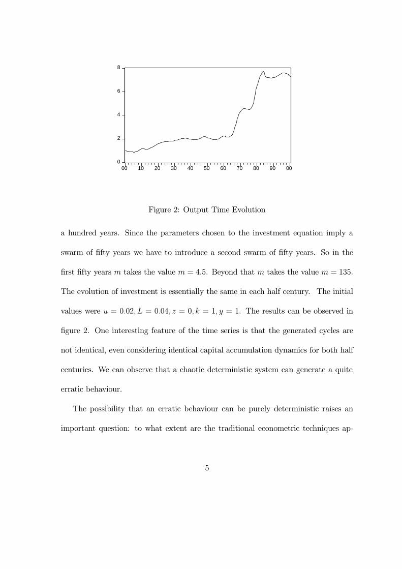
Figure 2: Output Time Evolution
a hundred years. Since the parameters chosen to the investment equation imply a
swarm of �fty years we have to introduce a second swarm of �fty years. So in the
�rst �fty years m takes the value m = 4:5. Beyond that m takes the value m = 135.
The evolution of investment is essentially the same in each half century. The initial
values were u = 0:02; L = 0:04; z = 0; k = 1; y = 1. The results can be observed in
�gure 2. One interesting feature of the time series is that the generated cycles are
not identical, even considering identical capital accumulation dynamics for both half
centuries. We can observe that a chaotic deterministic system can generate a quite
erratic behaviour.
The possibility that an erratic behaviour can be purely deterministic raises an
important question: to what extent are the traditional econometric techniques ap-
5
propriate to deal with this new issue? We will try to sketch the answer in the next
point.
2 An Econometric Application to Our Arti�cial Model
Blatt (1983) alerted to the dangerous consequences of an error in the identi�cation
of the stability properties of an economic system. He then asked if the traditional
econometric tools were a good instrument to analyze the stability of an economic
system. To answer this question he made a simple test.
He generated some economic time series with the help of a nonlinear, locally
unstable, macro-model Hicks proposed. With these arti�cial data he tried to estimate
the original model. The results are quite unpleasant: the estimated model did not
identify (not even close) the inherent instability of the original model. Basically, a
dynamically stable model was estimated and the endogenous cycles were attributed
to stochastic shocks, with no statistic evidence of misspeci�cation.
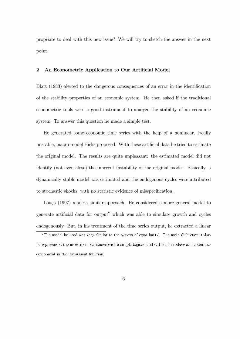
Louçã (1997) made a similar approach. He considered a more general model to
generate arti�cial data for output2 which was able to simulate growth and cycles
endogenously. But, in his treatment of the time series output, he extracted a linear
2The model he used was very similar to the system of equations 5. The main di¤erence is that
he represented the investment dynamics with a simple logistic and did not introduce an accelerator
component in the investment function.
6
trend3 and thenmodelled the residuals as a linear autoregressive process. The problem
with Louçã�s approach is that when one tries to apply usual econometric procedures to
time series data it is not possible to forget testing the stationarity of the series before
extracting a (linear) time trend. Depending on the results of that test extracting a
linear time trend may, or may not, be appropriate.
We tested the stationarity of time series represented in �gure 2 (the test used was
the ADF test and was applied after logarithmizing the series). According to the test
result, we could not reject the null hypothesis of nonstationarity for the log of the
output (LY ), while for the growth rate (DLY ) we reject the null hypothesis accepting
the growth rate4 to be stationary around a constant. So an applied econometrist
would not extract a linear trend to stationarize the series. He would rather consider
the growth rate of Y .
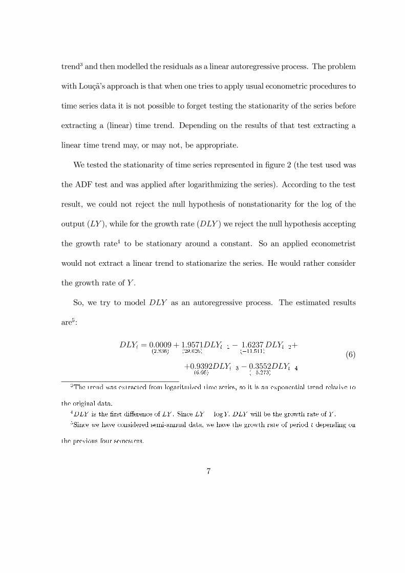
So, we try to model DLY as an autoregressive process. The estimated results
are5:
DLYt = 0:0009(2:836)
+ 1:9571(29:026)
DLYt¡1 ¡ 1:6237(¡11:511)
DLYt¡2+
+0:9392(6:66)
DLYt¡3 ¡ 0:3552(¡5:273)
DLYt¡4
(6)
3The trend was extracted from logaritmized time series, so it is an exponential trend relative to
the original data.
4DLY is the �rst di¤erence of LY . Since LY = logY; DLY will be the growth rate of Y .
5Since we have considered semi-annual data, we have the growth rate of period t depending on
the previous four semesters.
7

where the values in parenthesis are the t-statistics. The R-squared (and the adjusted
R-squared) is about 96%. The residuals show no evidence of serial correlation. The
number of lags chosen was based on the Akaike and Schwarz information criteria and
were strengthened by the fact that higher lags were not statistically signi�cant6.
It is interesting to note that equation 6 is a simple di¤erence equation with an
explicit analytic solution:
DLYt = 0:0104 + 0:6627t (A1 cos (1:4073t) +A2 sin (1:4073t))+
+0:8994t (A3 cos (0:2534t) +A4 sin (0:2534t))
(7)
where A1; A2; A3; and; A4 are arbitrary constants that can be determined with the
help of four initial conditions.
This estimated model �ts perfectly in Slutsky- Frisch�s paradigm: we have an
exogenous trend (determined by the constant 0.01042) and two di¤erent growth cycles
(one with 4: 5years and the other with 24: 8 years) aggregated additively. In �gure 3
we can see how this estimated model would work in the absence of stochastic shocks.
To explain the persistence of cycles in this model, Frisch would suggest the addition
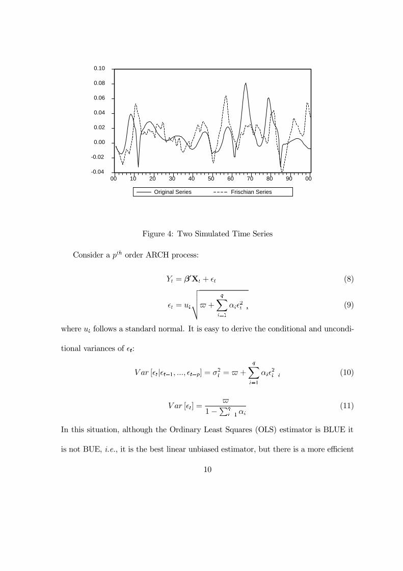
of a stream of exogenous shocks. This is what we do next. We add a stream of
exogenous shocks with mean zero and variance 0.0001444 to equation 6 with the help
of a normal random number generator7. In �gure 4 we compare the original arti�cial
6For example, if we introduced a �fth lag, its P-value would be 0.39.
7The variance was chosen in such a way that the original time series and this new time series
8

-0.015
-0.010
-0.005
0.000
0.005
0.010
0.015
0.020
00 10 20 30 40 50 60 70 80 90 00
Figure 3: The Estimated Model Dynamics
time series with the time series generated by the estimated model (augmented with
the stochastic shocks)8.
2.1 Problems with Heteroskedasticity
We have so far neglected the possibility of having heteroskedastic disturbances. In
traditional time series analysis it was usual to consider homoskedastic processes (as-
sociating heteroskedasticity to cross-sectional data). But, at least since Engle (1982),
one cannot put aside the possibility of having an Autoregressive Conditional Het-
eroskedasticity (ARCH) model or one of its extensions, as we shall see.
have the same variance.
8Although not reproduced here, we would have reached the same qualitative results if we had
applied the Hodrick-Prescott �lter instead and then �tted an autoregressive process to the residuals.
9
-0.04
-0.02
0.00
0.02
0.04
0.06
0.08
0.10
00 10 20 30 40 50 60 70 80 90 00
Original Series Frischian Series
Figure 4: Two Simulated Time Series
Consider a pth order ARCH process:
Yt = ¯0
Xt + ²t (8)
²t = ut
vuut$ +
qXi=1
®i²2
t¡i (9)
where ut follows a standard normal. It is easy to derive the conditional and uncondi-
tional variances of ²t:
V ar [²tj²t¡1; :::; ²t¡p] = ¾2t = $ +
qXi=1
®i²2
t¡i (10)
V ar [²t] =$
1¡Pq
i=1 ®i
(11)
In this situation, although the Ordinary Least Squares (OLS) estimator is BLUE it
is not BUE, i.e., it is the best linear unbiased estimator, but there is a more e¢cient
10
obs£R2 P-value
1st order 2.979 0.084
2nd order 15.199 0.001
3rd order 15.149 0.002
4th order 16.030 0.003
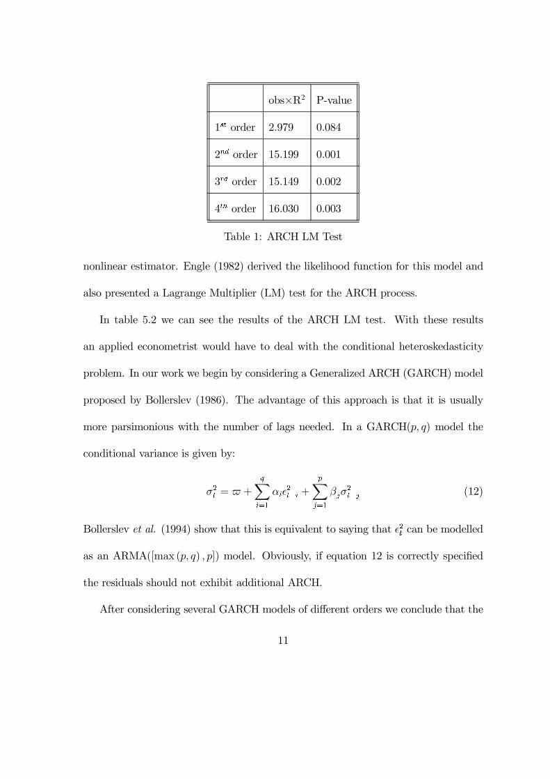
Table 1: ARCH LM Test
nonlinear estimator. Engle (1982) derived the likelihood function for this model and
also presented a Lagrange Multiplier (LM) test for the ARCH process.
In table 5.2 we can see the results of the ARCH LM test. With these results
an applied econometrist would have to deal with the conditional heteroskedasticity
problem. In our work we begin by considering a Generalized ARCH (GARCH) model
proposed by Bollerslev (1986). The advantage of this approach is that it is usually
more parsimonious with the number of lags needed. In a GARCH(p; q) model the
conditional variance is given by:
¾2t = $ +
qXi=1
®i²2
t¡i +
pXj=1
¯j¾2
t¡j (12)
Bollerslev et al. (1994) show that this is equivalent to saying that ²2t can be modelled
as an ARMA([max (p; q) ; p]) model. Obviously, if equation 12 is correctly speci�ed
the residuals should not exhibit additional ARCH.
After considering several GARCH models of di¤erent orders we conclude that the
11

standardized residuals continued to exhibit ARCH, indicating that equation 12 was
misspeci�ed.
Nelson (1991) proposed an Exponential GARCH (EGARCH) model. Equation 12
is replaced by:
ln¡¾2t
¢= $ +
qXi=1
µ®i
¯̄¯̄ ²t¡i
¾t¡i
¯̄¯̄+ °i
²t¡i
¾t¡i
¶+
pXj=1
¯j ln¡¾2t¡j
¢(13)
When we re-estimate equation 6, admitting that the conditional heteroskedasticity
follows an EGARCH(2; 4)9:
DLYt = 0:00003(19:830)
+ 3:0965(281:625)
DLYt¡1 ¡ 3:6082(¡135:434)
DLYt¡2
+1:8744(84:615)
DLYt¡3 ¡ 0:3679(¡55:842)
DLYt¡4
(14)
ln (¾2t ) = ¡ 7:2006
(¡14:975)+ 2:1347
(17:355)
¯̄̄²t¡1
¾t¡1
¯̄̄¡ 0:0650
(¡0:816)
²t¡1
¾t¡1
+1:8102(9:183)
¯̄¯ ²t¡2
¾t¡2
¯̄¯¡ 0:0242
(¡0:264)
²t¡2
¾t¡2
+0:0583(0:930)
ln¡¾2t¡1
¢+ 1:3331
(36:398)ln¡¾2t¡2
¢
¡0:1151(¡2:611)
ln¡¾2t¡3
¢¡ 0:5251
(¡16:551)ln¡¾2t¡4
¢
(15)
where the values in parenthesis are the z-statistics. As it can be seen, the results of
equation 14 do not di¤er substantially from the results obtained in equation 6. It
is easy to verify that the stability properties do not change. When the ARCH LM
test is applied to the standard residuals, the results are conclusive. As we can see in
9The order of the ARCH process was chosen, basically, with the help of the Akaike and Schwartz
information criterion, and with signi�cance tests.
12

obs£R2 P-value
1st order 0.009 0.924
2nd order 1.693 0.429
3rd order 1.936 0.586
4th order 2.096 0.718
Table 2: ARCH LM Test to EGARCH standard residuals
table 5.3, no economist would reject the null hypothesis of conditional homoskedastic
residuals. Even the Jarque-Bera normality test tends to accept the good speci�cation
of the model (the Jarque-Bera statistic has a value of 2.4 with a P -value of 0.3). So,
we would even accept the normality of the standard residuals.
Although we did not perform a battery of tests, so that we cannot be sure the
estimated model would pass in all speci�cation tests, we can see a tendency to accept
this wrong model. We say wrong because equation 14 represents a linear stable model,
when we know the true model is a nonlinear unstable one. Even equation 15 tells us
that, although the conditional variance of the residuals will vary with time, it will
stabilize, unless it is fed with exogenous shocks. The intrinsic instability of the model
is not captured by any of the components of the EGARCH estimates.
13

Figure 5: Dimension of Stochastic Processes vs Deterministic Processes
2.2 The BDS Statistic
2.2.1 Dimension of Stochastic Processes
Although nonlinear deterministic models can generate random processes, one impor-
tant di¤erence between deterministic and stochastic processes is that while determin-
istic processes have �nite dimension, stochastic processes have in�nite dimension.
We can see in �gure 5 the phase portrait of a chaotic deterministic series based on
the logistic equation (Yn+1 = 4Y
n(1¡ Y
n)) and of a stochastic series. It is easy to see
that while the deterministic process is one-dimensional, the stochastic series �lls out
the entire area. Thus the stochastic process is at least two dimensional. If we plot a
three-dimensional phase portrait we will conclude that the stochastic process �lls out
the entire cube and so on for higher dimensions. So a stochastic process approaches
an in�nite dimension.
14

2.2.2 The Correlation Dimension and the BDS Statistic
Based on the above notion of dimension Brock et al. (1987)10 propose a statistical
procedure to test departures from independently and identically distributed (i.i.d.)
observations.
Consider T observations of a time series (x1, x2, ..., xT ) after removing all non-
stationary components. De�ne them-histories of xt process as the vectors (x1; :::; xm),
(x2; :::; xm+1), ..., (xT¡m+1; :::; xT ). Now de�ne the correlation integral as the fraction
of the distinct pairs of m-histories lying within a distance " in the sup norm11:
C";m;T =1
(T ¡m+ 1) (T ¡m)
TXi=1
TXj=1
i 6=j
H¡"¡ supnorm
¡xi;xj
¢¢(16)
where xi = (xi; :::; xi+m¡1) and H (x) =
8>><>>:
0 if x � 0
1 if x > 0
.
Under some assumptions C";m;T converges to a limit C";m. The true correlation
dimension is given by d ln(C";m)d ln "
. It is possible to show that the correlation dimension
has the Hausdor¤ dimension as its upper bound. Ifd ln(C";m;T )
d ln "increases without bound
with m then one conclude that data is stochastic, ifd ln(C";m;T)
d ln "tends to a constant
10Brock, W. Dechert, W. and Sheinkman, J. (1987), �A Test for Independence Based on the
Correlation Dimension�, University of Winsconsin, Madison, University of Houston, and University
of Chicago, cit. in Brock et al. (1991).11Brock (1986) showed that the correlation dimension was independent of the choice of the norm,
so it is not restrictive to consider the sup norm.
15
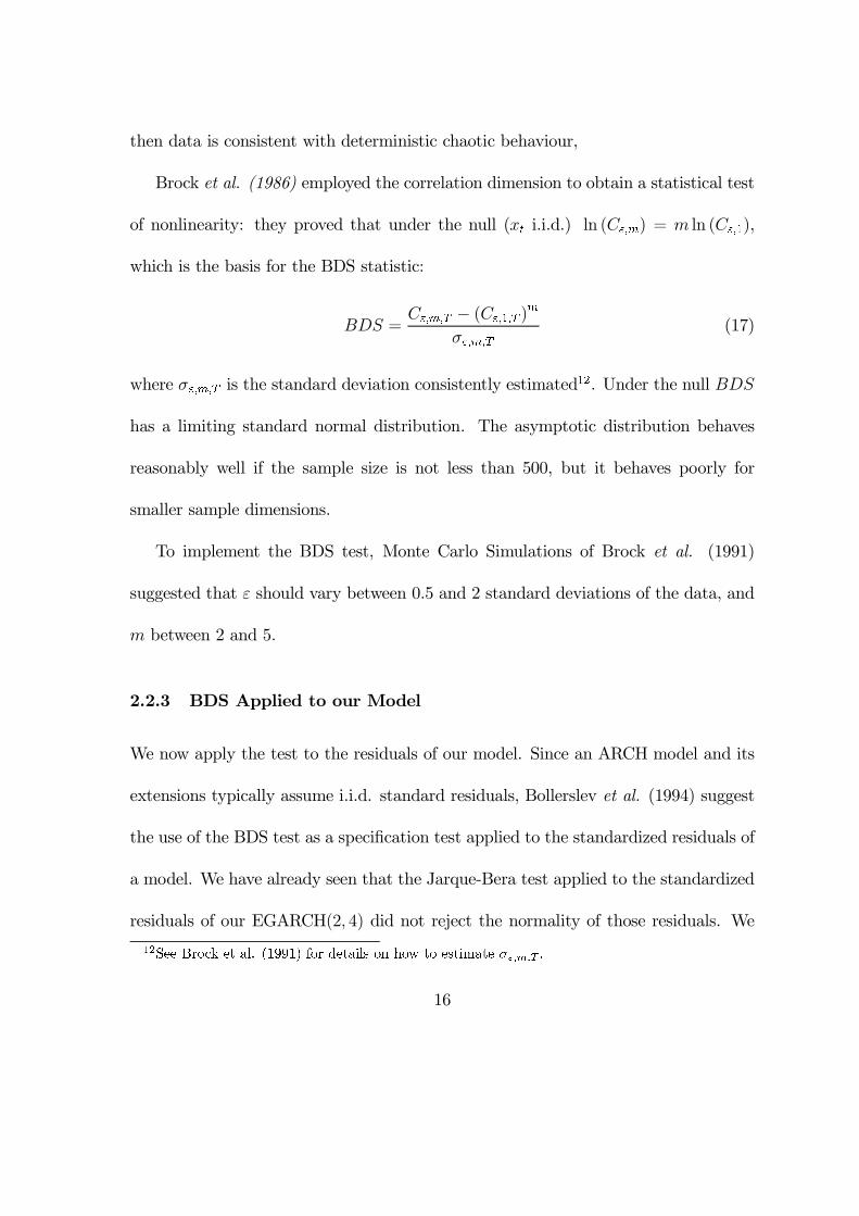
then data is consistent with deterministic chaotic behaviour,
Brock et al. (1986) employed the correlation dimension to obtain a statistical test
of nonlinearity: they proved that under the null (xt i.i.d.) ln (C";m) = m ln (C";1),
which is the basis for the BDS statistic:
BDS =C";m;T ¡ (C";1;T )
m
¾";m;T
(17)
where ¾";m;T is the standard deviation consistently estimated12. Under the null BDS
has a limiting standard normal distribution. The asymptotic distribution behaves
reasonably well if the sample size is not less than 500, but it behaves poorly for
smaller sample dimensions.
To implement the BDS test, Monte Carlo Simulations of Brock et al. (1991)
suggested that " should vary between 0.5 and 2 standard deviations of the data, and
m between 2 and 5.
2.2.3 BDS Applied to our Model
We now apply the test to the residuals of our model. Since an ARCH model and its
extensions typically assume i.i.d. standard residuals, Bollerslev et al. (1994) suggest
the use of the BDS test as a speci�cation test applied to the standardized residuals of
a model. We have already seen that the Jarque-Bera test applied to the standardized
residuals of our EGARCH(2; 4) did not reject the normality of those residuals. We
12See Brock et al. (1991) for details on how to estimate ¾";m;T :
16

m 2 3 4 5
" = 0:5¾ 13:85(0:00)
18:01(0:00)
25:44(0:00)
41:47(0:00)
" = ¾ 7:16(0:00)
7:14(0:00)
7:37(0:00)
7:80(0:00)
Table 3: BDS Test to the EGARCH(2,4) residuals
now apply the BDS test to the same residuals. Two di¢culties need to be faced with.
First, the small dimension of the sample. Second, the asymptotic distribution of the
test, which is strongly a¤ected by the �tting of the EGARCH model, and has uet
not been derived.To overcome both problems, we follow a procedure suggested by
Brock et al. (1991), also applied by Louçã (1997): after estimating the BDS statistic
we shue randomly the time series sample and then re-estimate the statistic. This
procedure is repeated 100 times. If the process is purely random the dimension of the
process will be unchanged and so will the estimated statistic. If the process is purely
deterministic, then shuing will destroy the correlation structure of the process. In
table 4.5 we can see the results achieved. In parenthesis we have the proportion of the
statistic values (obtained after reshuing) that are higher (in absolute value) than
the statistic applied to the original series. As we can see, the results of the statistic
point, correctly, to a misspeci�cation of the model.
17

2.2.4 Some Problems
The above results suggest that it is easy to determine whether a time series follows
a chaotic process or not. We must take this conclusion very carefully. First, the
rejection of the null hypothesis does not tell us anything about the alternative. For
example, the data generator process may be a stochastic nonlinear model and not a
chaotic deterministic model. Second, there is no practical distinction between a high
dimensional chaotic model and a pure stochastic model, so this test is only appropriate
to detect low dimensional chaos.
An interesting problem, particularly when we are analyzing macroeconomic time
series, is the problem with aggregate data. One of the �aws Schumpeter found in
Keynes� work was the use of aggregate functions (consumption, investment, etc.).
He argued aggregation could mask innovative processes which are speci�c to some
industries. Goodwin (1991) agreed to this idea and defended the use of large mul-
tidimensional systems even though, unfortunately, for simplicity sake, he presented
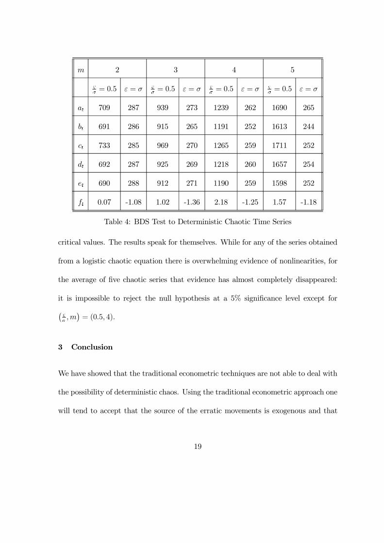
an aggregated model.To illustrate this problem we can see in table 6 the BDS test
applied to �ve di¤erent series13 and to their average (ft =at+bt+ct+dt+et
5). Since the
sample has 2000 observations, we can use the standard normal distribution to �nd the
13The series were generated according to the formula: xt = 4xt¡1 (1¡ xt¡1). The initial values
for series at; bt; ct; dt; and et were, respectively, 0.1, 0.2, 0.3, 0.4, and 0.49. 3000 observations were
generated, being the �rst 1000 thrown away.
18
m 2 3 4 5
"
¾= 0:5 " = ¾ "
¾= 0:5 " = ¾ "
¾= 0:5 " = ¾ "
¾= 0:5 " = ¾
at 709 287 939 273 1239 262 1690 265
bt 691 286 915 265 1191 252 1613 244
ct 733 285 969 270 1265 259 1711 252
dt 692 287 925 269 1218 260 1657 254
et 690 288 912 271 1190 259 1598 252
ft 0.07 -1.08 1.02 -1.36 2.18 -1.25 1.57 -1.18
Table 4: BDS Test to Deterministic Chaotic Time Series
critical values. The results speak for themselves. While for any of the series obtained
from a logistic chaotic equation there is overwhelming evidence of nonlinearities, for
the average of �ve chaotic series that evidence has almost completely disappeared:
it is impossible to reject the null hypothesis at a 5% signi�cance level except for
¡"
¾;m
¢= (0:5; 4).
3 Conclusion
We have showed that the traditional econometric techniques are not able to deal with
the possibility of deterministic chaos. Using the traditional econometric approach one
will tend to accept that the source of the erratic movements is exogenous and that
19

the system is dynamically stable, even though the model is known to be inherently
unstable.
Another problem is that speci�c econometric techniques, designed to deal with
the possibility of deterministic chaos, are not as powerful as one might wish: we saw
that aggregation can hide evidence of nonlinearities, a problem that can arise in many
macroeconomic time-series
References
Blatt, J.M. (1983), Dynamic Economic Systems � a Post-Keynesian Approach,
Armonk, New York.
Bollerslev, T. (1986), �Generalized Autoregressive Conditional Heteroskedastic-
ity�, Journal of Econometrics, vol.31, pp. 307-327.
Bollerslev, T., Engle, R. and Nelson, D. (1994), �ARCH Models�, in Handbook
of Econometrics � Volume IV, Engle, R. and McFadden, D. (editors), chapter
50, pp. 2959-3038, Elsevier.
Brock (1986), �Distinguishing Random and Deterministic Systems: Abridged
Version�, Journal of Economic Theory, vol. 40, pp. 168-195.
Brock, W., Hsieh, D. and Baron, B. (1991), Nonlinear Dynamics, Chaos, and
Instability: Statistical Theory and Economic Evidence, Cambridge: MIT Press.
20
Engle, R.F. (1982), �Autoregressive Conditional Heteroskedasticity with Esti-
mates of the Variance of U.K. In�ation�, Econometrica, vol. 50, pp. 987-1007
Goodwin. R. (1967), �A Growth Cycle�, in Socialism, Capitalism and Economic
Growth, C. H. Feinstein (editor), pp. 54-58, Cambridge University Press.
Goodwin, R. (1991), �Economic Evolution, Chaotic Dynamics and the Marx-
Keynes-Schumpeter System�, in Rethinking Economics: Markets, Technology
and Economic Evolution, chapter 9, Edward Elgar, pp. 138-152.
Nelson, D. (1991), �Conditional Heteroskedasticity in Asset Returns: A New
Approach�, Econometrica, vol. 59, 347-370
Stone, R. (1990), �A Model of Cyclical Growth�, in Nonlinear and Multisectoral
Macrodynamics: Essays in Honour of Richard Goodwin, Velupillai, K. (editor),
Chapter 6, pp. 64-89, Macmillan.
21


