Page 1
Imperial College London
Department of Theoretical Physics
The AdS/CFT correspondenceand condensed matter physics
Adam John Ready
17 September 2012
Supervised by Prof. Daniel Waldram
Submitted in partial fulfillment of the requirements for the degree of
Master of Science of Imperial College London
Page 2
Contents
1 Introduction 2
2 The AdS/CFT correspondence: a review 4
2.1 The Weinberg-Witten theorem . . . . . . . . . . . . . . . . . 4
2.2 The holographic principle . . . . . . . . . . . . . . . . . . . 9
2.3 The ’t Hooft limit . . . . . . . . . . . . . . . . . . . . . . . . 10
2.4 Extra dimensions and the renormalisation group . . . . . . . 14
2.5 Anti-deSitter space and conformal field theories . . . . . . . 17
2.6 CFT conditions for duality . . . . . . . . . . . . . . . . . . . 20
3 Condensed matter systems and holography 22
3.1 The Bose-Hubbard model . . . . . . . . . . . . . . . . . . . 22
3.2 The phases of the Bose-Hubbard model . . . . . . . . . . . . 23
3.3 Quantum phase transitions . . . . . . . . . . . . . . . . . . . 28
3.4 The coherent state path integral . . . . . . . . . . . . . . . . 30
3.5 Extracting the conformal field theory . . . . . . . . . . . . . 35
3.6 Motivation for holographic methods . . . . . . . . . . . . . . 38
3.7 Holographic analysis . . . . . . . . . . . . . . . . . . . . . . 40
4 Conclusion 47
1
Page 3
Chapter 1
Introduction
The AdS/CFT correspondence is one of the most influential conjectures that
has been discovered recently in theoretical physics. It was first stated by
Juan Maldacena [16] for a particular highly symmetric quantum field theory
called N = 4 super Yang-Mills in four space-time dimensions, and a string
theory called type IIB formulated on a particular space-time background.
At a basic level it states that a quantum theory of gravity, such as string
theory, is dual to a lower dimensional quantum field theory without gravity.
Just the statement alone opens up many speculative ideas and many
questions. For instance this could be a way of learning more about quantum
gravity, a field that it notoriously challenging with many candidate theories
[5]. Another possible use of the correspondence is to use it in the opposite
direction: to use developments in string theory to describe certain classes
of quantum field theories. This is the line of argument of this dissertation,
which will consider quantum field theories which describe condensed matter
systems under very specific physical conditions [26].
The condensed matter systems in question will be those that whose be-
havior can be described by the boson-Hubbard model, namely bosons whose
dynamics are confined to sites of a lattice [28, section9]. The reason that the
boson-Hubbard model is of interest is because at a certain quantum critical
point between quantum phases of matter the system can be described by a
quantum field theory with just the right symmetries to apply the AdS/CFT
2
Page 4
correspondence [29]. It is a remarkable duality between gravitational sys-
tems and ultra-cold atoms, which is only possible because of the loss of a
physical length scale in the condensed matter system. It is this that allows
the duality to be conjectured, and the reason that systems that naively
have completely different physical distance scales are actually identical by
the absence of scale.
The structure of this dissertation is to introduce the AdS/CFT corres-
pondence in section 1 in a way that makes it easier to apply to condensed
matter systems. Issues regarding the degrees of freedom, the Weinberg-
Witten theorem [37] which appears to forbid such a duality, and the descri-
bing the extra dimensions of the gravity theory will be discussed.
Section 2 will introduce the boson-Hubbard model and show that the low
energy limit of the model can be described by a particular type of quantum
field theory amenable to a gravity description via AdS/CFT. Finally the
duality will be used to predict physical properties of the system that other
theories have been unable to provide [29]. The dissertation will conclude
with additional developments that have been made, and scope for further
research in this field.
3
Page 5
Chapter 2
The AdS/CFT correspondence: a re-
view
This section will serve to motivate the AdS/CFT correspondence by asking
questions around the idea of a gauge-gravity duality. The first few sections
will introduce the Weinberg-Witten theorem and the holographic principle
which places restrictions on the form such a duality could take, such as
the gravity theory having more space-time dimensions than the field theory.
After introducing the ’t Hooft large N limit the following sections will match
the extra dimensions using the renormalisation group and the symmetries
of the two theories by observation. The concluding section considers what
conditions a QFT needs to have a gravity dual with an asymptotically AdS
background besides conformal invariance.
2.1 The Weinberg-Witten theorem
When quantizing gravity it is inevitable that a spin 2 particle will emerge
from the procedure commonly referred to as the graviton. When comparing
a quantum gravity theory with a QFT a natural question would be is it
possible to have a spin 2 particle in a QFT? In principle it seems one could
form a bound state of say two gauge bosons such that they behave like a
spin 2 particle. The theorem first proved by Steven Weinberg and Edward
Witten [37] sheds light on this question:
4
Page 6
Theorem 2.1.1 A QFT with a Poincare covariant conserved stress tensor
T µν forbids massless particles of spin j > 1 which carry momentum (i.e.
P µ =∫d3x T 0µ 6= 0.)
An outline of the proof the Weinberg-Witten theorem will be provided
here based on the arguments of the original paper [37] and a review by
Florian Loebbert [15]. Additional details, especially those concerning nor-
malization of one particle states can be found in the aforementioned review.
The proof will be divided into two parts, the first will (i) show that the
matrix elements corresponding to the the tensor T :
〈p′,±j|T µν |p,±j〉 (2.1.1)
cannot vanish in the limit in which p′ → p. The second part (ii) will
show that the same matrix elements must vanish under the assumptions of
the theorem if the helicity of massless particles and j > 1 for the matrix
elements associated with T.
(i) To show the first result we will make use of the 4-momentum ope-
rator associated with T µν in the statement of the theorem. If the massless
particles are charged under T then their eigenvalues with respect to T must
be non-zero. This will be one of the crucial assumptions of the theorem.
We will define the 4-momentum eigenvalues of pure momentum 1-particle
massless states as:
P µ|p,±j〉 = pµ|p,±j〉. (2.1.2)
All 1-particles states can be described as linear combinations of these
pure momentum eigenstates with their momentum given by a linear combi-
nation of the same eigenstates’ eigenvalues. We can then define the matrix
5
Page 7
elements above as follows:
〈p′,±j|P µ|p,±j〉 = pµδ(3)a (p′ − p) (2.1.3)
where we have normalized the momentum eigenstates using δa the nascent
delta function defined in terms of the delta function as lima→0 δ(3)a (p′−p) =
δ(3)(p′ − p). Normalizing using nascent delta functions ‘smears out’ the
single particle state excitations allowing a more physical interpretation of
results found using this convention as opposed to using ordinary δ-functions.
For more details see [15]. The use of smeared out delta-functions corres-
ponds to integrating not over all space, but finite volumes. The definition
of the nascent delta-function above is defined by integrating it over a ball of
radius 1/a which becomes an infinite sized ball in the limit a→ 0. We will
use δa to define the 4-momentum operator as in the theorem over a finite
volume:
〈p′,±j|P µ|p,±j〉 =
∫Va
d3x〈p′,±j|eiP·xT 0µ(t,0)e−iP·x|p,±j〉
=
∫Va
d3xei(p′−p)·x〈p′,±j|T 0µ(t,0)|p,±j〉
= (2π)3δ(3)a (p′ − p)〈p′,±j|T 0µ(t,0)|p,±j〉.(2.1.4)
If we compare this result with our previous result ?? we obtain the
identity:
limp′→p〈p′|T 0µ|p〉 =
pµ
(2π)3. (2.1.5)
We can generalize this result using Lorentz covariance:
limp′→p〈p′|T µν |p〉 =
pµpν
E(2π)3. (2.1.6)
Because we assumed that the eigenvalues of our one-particle states were
non-zero these matrix elements must be non-zero.
6
Page 8
(ii) To show the second result we will first consider this relation for
light-like momenta p′ and p:
(p′ + p)2 = (p′)2 + p2 + 2(p′ · p) = 2(p′ · p)
= 2(p′ · p− |p′||p|
= 2|p′||p|(cos(φ)− 1) ≤ 0. (2.1.7)
where φ is the angle between 3-momenta p′ and p. Because we are
considering the limit p′ → p the case of φ = 0 is not applicable, hence
throughout the rest of this proof we will assume φ is non-zero. First by
Poincare covariance of our states we will choose a frame such that they
have opposite 3-momentum: p = (|p|,p), p′ = (|p|,−p). Next we will
consider a rotation of θ about the 3-momentum p axis. The one-particle
states transform as:
|p,±j〉 → e±iθj|p,±j〉
|p′,±j〉 → e∓iθj|p′,±j〉. (2.1.8)
Thus the matrix elements transform as:
〈p′,±j|T µν(t,0)|p,±j〉 → e±2iθj〈p′,±j|T µν(t,0|p,±j〉. (2.1.9)
Another way we can define a rotation is as fundamental representations
of the Lorentz group acting on the matrix T . We can compare the first
and this description of the rotation in the same way we compare active and
passive transformations. The first description of the rotation transforms the
basis states, whilst the second description transforms the operators that act
upon the states. The second description can be written as:
〈p′,±j|T µν(t,0)|p,±j〉 → Λ(θ)µρΛ(θ)νσ〈p′,±j|T ρσ(t,0|p,±j〉. (2.1.10)
7
Page 9
Equating both transformation descriptions:
e±2iθj〈p′,±j|T µν(t,0|p,±j〉 = Λ(θ)µρΛ(θ)νσ〈p′,±j|T ρσ(t,0|p,±j〉. (2.1.11)
We now note that because Λ is a representation of a rotation in the
Lorentz group its eigenvalues can only be either eiθ or 1. This constrains
the values j can possibly take to either 0, 1/2, or 1, for any other value the
matrix elements of T vanish. We chose a reference frame for our analysis,
but using Poincare covariance of T and Poincare invariance of helicities this
result carries over to all Lorentz frames of reference.
Hence for a Poincare covariant tensor T µν it follows that:
limp′→p〈p′,±j|T µν |p,±j〉 = 0 for j > 1. (2.1.12)
Hence the first result shows that 〈p′|T µν |p〉 cannot vanish in the limit
p′ → p and the second result show that 〈p′|T µν |p〉 must vanish if j > 1,
hence we obtain the result that massless particles with helicity j > 1 vanish
in a Poincare covariant QFT with covariant T µν .
This appears to forbid any spin-2 particle, even bound states, which rules
out the graviton, since any particle with spin-2 shares all the properties
of the graviton [15, page 18]. However, there is a window provided by
general relativity. For any stress-energy tensor of a gravity theory that
obeys Einstein’s field equations T µν ∝ δSδgµν
where S is the Einstein-Hilbert
action. This vanishes by the equations of motion of the gravity theory.
Thus the stress energy tensor for the full gravity theory vanishes and so the
Weinberg-Witten theorem no longer applies since a non-vanishing stress-
energy tensor was assumed.
We can still have massless particles with momentum since the stress-
energy tensor is the sum of the stress-energy tensor of the QFT plus the
stress-energy of just pure gravity, T µν = T µνQFT +T µνQG. From the holographic
8
Page 10
principle we will assume that the QFT lives on the boundary of the whole
space-time with gravity living in the ’bulk’ of the space-time. T µνQFT is
Poincare covariant on the boundary, but need not be in the bulk, hence
the Weinberg-Witten theorem applies on the boundary and so there can
be no massless particles of spin > 2 there, but in the bulk, since there
is no Poincare covariant tensor except the total one which vanishes, the
Weinberg-Witten theorem does not apply. This means a graviton composite
particle can exist, but not on the boundary of the space-time where the QFT
resides. It must live in the bulk with at least one extra dimension necessary
to describe it, corresponding to the radial distance from the boundary.
2.2 The holographic principle
The holographic principle was first proposed by Gerard ’t Hooft [35] with
additional contributions to bring it into the field of string theory by Leonard
Susskind [33]. Also many of the ideas have been discussed by Charles Thorn
[33]. The result stems from the work of Bekenstein and Hawking that states
that black holes not only have a temperature [12], but also an entropy [2]
that is proportional to the black hole’s surface area A:
SBH =1
4
c3kBG~
A (2.2.1)
where c is the speed of light, kB is Boltzmann’s constant, G is Newton’s
gravitational constant, and ~ is Planck’s constant. The only other result
that the holographic principle requires is simply that if enough energy ac-
crues within a small enough volume the matter will undergo gravitational
collapse and form a black hole. This result can be seen in the canonical
theoretical example of the Schwarzschild solution, but also the more ge-
neral cases of rotating Kerr and charged Reissner-Nordstrom solutions of
Einstein’s field equations, see [36, pages 312, 158, and 317] for more details.
Both of these results together imply the holographic principle, that the
maximum entropy in a space-time volume is proportional to its surface area.
9
Page 11
This is exactly the entropy of the largest black hole that can occupy this
volume. To see why this is consider a volume of space-time V with surface
area A and entropy S > SBH ∝ A. Assume also that the energy in this
volume is less than that of a black hole (otherwise the energy density would
cause gravitational collapse and a black hole would be formed). Now add
energy in any form to the volume so that the energy density reaches the va-
lue at which a black hole is formed. The configuration we have now has less
entropy than the one we started with, since S > SBH . This violates the se-
cond law of thermodynamics, so rather than do that, ’t Hooft assumed that
a black hole is the configuration with the highest entropy per unit volume,
and thus the maximum entropy in a space-time volume is proportional to
the surface area of the volume.
This is far smaller than the entropy of a local QFT on the same space,
even with some UV cutoff equivalent to a length scale such as the Planck
length lP . Such a theory would have a number of states Ns ∝ nV/l3P (where
V is the spatial volume of the QFT and n is the number of states per site)
with maximum entropy ∝ ln(Ns) [18, 33]. Hence for a quantum theory of
gravity to be dual to a QFT, the QFT would have to be formulated on a
a lower number of dimensions, at least one dimension lower, so that the
degrees of freedom can at least in principle be equated.
2.3 The ’t Hooft limit
The ’t Hooft large N limit was first discovered by Gerard ’t Hooft in 1974
[34] whilst trying to find a way of simplifying the calculations of quantum
chromodynamics. He used the rank of the gauge group as a variable of the
theory, hence instead of SU(3) he used SU(N) for N an integer parameter.
As the name suggests by taking N to approach infinity the theory drastically
simplifies calculations of the theory in an illuminating fashion. Consider the
Lagrangian of the theory for a gauge field Aaµ in the adjoint representation
10
Page 12
of SU(N):
L = − 1
4g2YMtr(FµνF
µν) (2.3.1)
where F aµν = ∂µA
aν − ∂νA
aµ − iεabcAbµA
cν such that µ, ν = 0, 1, 2, 3 and
a = 1, . . . N2 − 1.
The field A has been defined differently from the usual form in the follo-
wing way Aaµ → g−1YMAaµ so that in this form the field strength is independent
of the gauge coupling. This form will become useful later in this section.
If we expand the Lagrangian out we see that the theory has 3-point and
4-point interaction vertices. Now consider the two vacuum diagrams (i) and
(ii):
(a) (b)
Figure 2.1: The connected vacuum diagrams associated with four 3-point
interactions.
To work out their dependence on N and the coupling gYM we need
to establish some rough Feynman rules. From the Lagrangian the kinetic
term has a factor of g−2YM in front of it, hence by inverting it to get the
propagator we infer that the propagator of the theory is proportional to
g2YM . Each of the interaction vertices has a factor of g−2YM in front of it,
hence each interaction vertex is proportional to g−2YM . Finally there is a
factor of N given for each sum over colour indices. One can work this out
by splitting the diagrams into propagators and vertices, use the Feynman
rules given by the Lagrangian, and count the number of sums. Using these
11
Page 13
Figure 2.2: A single line representing an adjoint field propagator can be
split into a pair of oppositely oriented lines representing a fundamental-
anti-fundamental product.
rules diagram (i) has associated with it a factor of g4YMN4 and diagram (ii)
has a factor of g4YMN2.
As N is taken towards infinity it will be useful to take the coupling gYM
to zero such that the quantity g2YMN = λ remains fixed. When we do this
2.1(a) with coefficient λ2N2 dominates over (b) with coefficient λ2. The
dominance of planar diagrams such as that of (a) over (b) occurs for all
diagrams with similar number of vertices and propagators. This is the ’t
Hooft large N limit. To see how this limit relates to string theory we’ll
introduce a technique invented by ’t Hooft called double line notation to
keep track of which classes of diagrams we keep and which we ignore. We
consider each gauge field or ‘gluon’ propagator that transforms in the adjoint
representation of SU(N) as a “quark anti-quark” pair that transforms in
the product of the fundamental and the anti-fundamental of SU(N), since
the adjoint can be thought of as roughly the product of the fundamental
and anti-fundamental. Diagrammatically this corresponds to replacing each
gluon propagator with two parallel lines with opposite orientations, the
fundamental and anti-fundamental going forwards and backwards in time
respectively.
This alteration also changes the interaction vertices in the obvious way,
so that the vacuum diagrams we drew above can be drawn using double
line notation as in 2.3(a) and (b). In this notation we see explicitly that the
factors of N correspond to the number of loops in the diagram: there are
four in (b), but only two in (b).
12
Page 14
(a) (b)
Figure 2.3: The connected vacuum diagrams associated with four 3-point
interactions drawn using double line notation.
This notation is said to ’polygonize’ the Feynman diagrams, the Feyn-
man diagrams provide a ’polygonization’ of a 2-dimensional surface. To
make this relation between diagrams and polygons more precise we will re-
late exactly the vertices of the Feynman diagrams to the vertices of the
polygons, the propagators to the edges, and the loops in the double line
notation to the faces. This means that any polygon with V vertices, E
edges, and F faces corresponds to a Feynman diagram, which according to
the Feynman rules above is proportional to:
(g2YM)E(g−2YM)V (N)F = λE−VNV−E+F . (2.3.2)
Note that the exponent of N , V − E + F is the Euler character χ
of the polygon, a well-known topological invariant used for classifying 2-
dimensional surfaces. For closed Riemann 2-surfaces χ = 2− 2g where g is
the genus, the number of holes, associated with the Riemann surface. Hence
any perturbation expansion can be written as
∞∑g=0
Nχ(g)
∞∑i=0
cg,iλi =
∞∑g=0
fg(λ)Nχ(g). (2.3.3)
The expansion is ordered by the Euler character of each contribution.
In the large N limit the planar diagrams, diagrams that can be drawn on
a sphere, with g = 0 will dominate all higher genus contributions. If we
13
Page 15
compare this expansion to string theory it too involves a double sum in
terms of string theory’s two parameters: the string coupling gs and the
string tension α′. By comparing both sums we identify gs with 1/N and α′
with λ giving a formal analogy between string theory and SU(N) QCD.
A subtlety to point out is that it has been assumed that the gauge group
was SU(N), but the expansion has been carried out as if the gauge group
is U(N) and not SU(N). This is valid up to leading order since U(N) has
N2 generators whereas SU(N) has N2−1 generators which can be equated
for large N at leading order, but at sub-leading order the difference must
be taken into account. Note also that this procedure can be applied for
any other gauge group, for example SO(N) or Sp(N), however since these
groups do not have conjugate representations the approach used to obtain
the ’t Hooft limit will differ. The natural question that arises when studying
the ’t Hooft limit is can SU(N) QCD be constructed as a string theory?
So far all efforts have been unsuccessful, but attempting to do so has led to
the AdS/CFT correspondence.
2.4 Extra dimensions and the renormalisation group
The Weinberg-Witten theorem seems to effectively forbid the notion of a
spin 2 particle in a QFT with Poincare covariance. To get around it we
concluded in accordance with the holographic principle that the spin 2 ‘gra-
viton’ does not live in the QFT, but in a gravity theory formulated in a
higher number of space-time dimensions. But how does this extra dimen-
sion manifest itself in the QFT? If a QFT and a quantum theory of gravity
are dual to each other this additional degree of freedom required by the
graviton must have a description in the QFT. The answer to this question
makes use of the renormalisation group (RG).
The renormalisation group is related to the procedure known as renor-
malisation. Renormalisation is a means of dealing with the infinities or
ultraviolet (UV) divergences present and seemingly intrinsic to QFTs whe-
14
Page 16
never physical quantities are computed. The problem involves space-time
integrals that are necessarily evaluated over all of space-time where quan-
tum fields are defined. By introducing a UV cut-off, usually denoted Λ,
it is possible to truncate all energy/momentum space integrals used to the
calculate physical observables of the theory. By systematically noting the
dependence of all correlation functions on the cut-off Lambda it can be
shown whether the QFT depends upon Λ in a finite or infinite number of
ways. If the QFT is renormalisable not only is the Λ dependence finite,
but also the number of times Λ appears is less than or equal to the number
of couplings of the theory. If this is the case the UV divergences can be
‘absorbed’ into the definitions of the couplings, now called ‘bare’ couplings,
and a new set of finite couplings can be determined called ‘renormalised’ or
‘physical’ couplings. These couplings can be measured, so that calculations
which depend upon the physical couplings rather than the bare couplings
yield finite results for physical quantities. Not only are they finite, in the
case of QED they are very accurate [23, page 198].
The cut-off scale Λ is key to the concept of the renormalisation group.
Because momentum and position are conjugate variables in quantum theory
plus energy and momentum are related in the same way as space and time
are related by relativity, an energy scale defines a conjugate length scale.
The length scale associated with the cut-off can be imagined as a resolution
scale used to describe a physical system, much like a digital camera used
to observe physical objects has a resolution associated with the number of
pixels of data the camera uses. If the cut-off scale of the theory is changed
then the parameters ( the couplings) change as well as the degrees of freedom
in the form of fields. This change is described by a group action, in that
any energy scale is accessible by any other via one of these transformations;
hence the name renormalisation group.
One of the most important equations associated with the renormalisation
group is the rate of change of the couplings with respect to a change in the
15
Page 17
energy scale which is called the Beta function of the theory:
β(g(Λ)) =dg
dΛ(Λ) (2.4.1)
An important thing to note about this relation is that it depends locally
on the value of the energy scale Λ. This means that to know how the
coupling changes we don’t need to know about the coupling in the high
energy UV or in the low energy infra-red (IR), all we need is local knowledge
to work out the beta function locally. This locality is reminiscent of space-
time coordinates, since in general relativity to compute local quantities only
the local geometry of space-time needs to be taken into account. Hence it
seems possible to associate the extra dimensions of the gravity theory with
the energy scale of the renormalisation group.
Figure 2.4: The energy scale can be viewed as a resolution scale of the
theory, hence there is a higher resolution at the ultra-violet energy scale
and lower at the infra-red.
A natural theory to consider is one for which the couplings don’t change
at all with energy scale, i.e. the beta function is zero. Such QFTs that
16
Page 18
realize this condition are thus scale invariant. A special subset of the scale
invariant QFTs called conformal field theories (CFTs) have a much stronger
set of conformal symmetries. As the name suggests are an essential part of
the AdS/CFT correspondence as the following section will discuss.
2.5 Anti-deSitter space and conformal field theories
An important concept in the AdS/CFT correspondence and gauge-gravity
duality in general is how the geometry of the gravity theory gives rise to
additional symmetries and how these manifest themselves in the quantum
field theory. In the particular case of the AdS/CFT correspondence the gra-
vity theory has a space-time background can be described by asymptotically
anti-deSitter (AdS) space. This is dual to a special subset of quantum field
theories call conformal field theories (CFTs). These terms will be explained
in the following section and the relation between their symmetries will be
motivated.
Anti-deSitter space-time (AdS) is a space-time with constant negative
curvature. It is the Lorentzian analogue of a hyperbolic space just as Min-
kowski space-time is the Lorentzian analogue of Euclidean space. To des-
cribe AdS space in (d+1)-dimensions one can embed it as a hyperbolic
hyper-surface in (d+2)-dimensions with embedding coordinates (X−1, X0,X =
X1, . . . , Xd) as:
−X2−1 −X2
0 + X ·X = −R2 (2.5.1)
where R is the AdS radius. This equation makes the symmetry group
of AdS space apparent, which is the SO(2, d). This equation can be solved
using Poincare coordinates:
17
Page 19
X−1 =1
2z(z2 +R2 + x2i − t2))
X0 =R
zt
Xi =R
zxi , i ∈ (1, . . . , d− 1)
Xd =1
2z(z2 −R2 + x2i − t2)) (2.5.2)
which yields the metric:
ds2 = (R
z)2[ηµνdx
µdxν + dz2]. (2.5.3)
An advantage of describing AdS space locally using Poincare coordinates
is that the constant z hypersurfaces are just copies of Minkowksi space, a
useful feature that motivates the AdS/CFT correspondence statement that
the CFT can be said to live on the bounding surface of AdS space.
The boundary of AdS space at z = 0 is an important thing to notice. To
get to the boundary from a finite value of z requires traversing an infinite
proper distance, however massless particles can still reach the boundary in a
finite time. For flat Minkowski space the boundary can only be reached for
time-like and null geodesics in an infinite proper time, so for most practical
situations boundary conditions can be trivial, i.e. all degrees of freedoms
such as fields vanish at infinity. However in the case of AdS space the
boundary conditions cannot always be trivial, they need to be specified
when setting up an physical problem, as well as initial conditions of the
degrees of freedom, on AdS space. These boundary conditions are a crucial
aspect of the AdS/CFT correspondence. A possible boundary condition
is that the space-time is asymptotically AdS, i.e. as one approaches the
boundary in the limit z → 0 the space looks locally like it has constant
negative curvature.
Conformal field theories have the usual Poincare group symmetries of
translations, rotations, and boosts, but are also invariant under scale trans-
18
Page 20
formations such as x → x/b and what are called special conformal trans-
formations. It can be shown by considering the Lie algebra of CFTs that
the special conformal transformations act like the translations, and together
with scale transformations CFTs are invariant under local scale transforma-
tions of the form
xµ → xµ
b(x)(2.5.4)
where b(x) ∈ R depends upon space-time position. Scale invariance is
a subset of these local symmetries when b is constant. If one considers the
Lie algebra of a conformal field theory one finds that it is the Lie algebra
of SO(2, d). As stated in the previous section, because CFTs are invariant
under spatial scaling they are also invariant under changes in the energy
scale, hence the beta function of any CFT vanishes, β(g) = 0.
Motivated by the previous section let’s consider a QFT that is scale
invariant, i.e. with a vanishing beta function, and use the energy scale
of the theory u as an additional coordinate to construct a metric for the
gravity theory. Using scale invariance the metric has to be invariant under
scale transformations x→ x/b, with u transforming u→ ub by dimensional
analysis. The metric must also preserve Poincare invariance. Imposing
these constraints results in the metric:
ds2 = (uL)2ηµνdxµdxν + (
du
u)2L2 (2.5.5)
where L and L are lengths. Under the scaling transformation u → LLu
we remove the dependence on L and the metric takes the form:
ds2 = (uL)2ηµνdxµdxν + (
du
u)2L2. (2.5.6)
We can make one more final coordinate change to bring the metric into
a form that makes the scale invariance more apparent. If we swap u with a
19
Page 21
length scale z = 1/u then the metric takes the form:
ds2 = (L
z)2[ηµνdx
µdxν + dz2]. (2.5.7)
This is in exactly the same form as the AdS metric in Poincare coor-
dinates with the identification R = L. Another thing to note is that the
symmetry group of AdS space in (d+1) dimensions and a CFT in d dimen-
sions are both SO(2, d). This motivates the result that a scale invariant
quantum field theory with a gravity dual can also be described by a confor-
mal field theory.
2.6 CFT conditions for duality
As the previous section clearly demonstrates, a CFT is a strong indicator
that a field theory has a dual description in terms of a quantum theory of
gravity formulated on an asymptotically AdS background. But are there
any additional conditions on the field theory side for an AdS/CFT type
correspondence? This question was considered by Polchinski et al [24] using
bulk locality to set conditions on the CFT. Arguing backwards they came
up with a conjecture based on the maximal set of necessary conditions for
a gauge-gravity duality.
The conjecture is: any CFT that has a large-N expansion, and in which
all single-trace operators of spin greater than two have parametrically large
dimensions, has a local bulk dual , [24].
The first condition we have already encountered in the form of the ’t
Hooft limit. This particular kind of large-N limit allows correlation function
contributions to be written as a perturbative expansion in terms of the genus
of the corresponding Feynman diagrams. The above condition requires that
any CFT must have some form of large-N limit such that this is the case.
The large-N limit on the gravity theory side is the limit in which the theory
becomes classical, which in the case of string theory means that the theory
20
Page 22
is well understood.
The second condition refers to single-trace operators which are dual to
single particle states in the bulk. Because no field theory we have encoun-
tered so far encourages operators at low-energy with spin greater than two
it would seem necessary that their presence in our field of experimental vi-
sion must be suppressed. If these states had a large number of dimensions
beyond the four we observe at low energy, the presence of these operators
would be sufficiently suppressed.
The second condition can be motivated using an important result from
the duality and considerations from string theory. The AdS/CFT corres-
pondence relates single trace operators in the CFT with scaling dimension
∆ to single particle field excitations in the bulk gravity theory of mass m
via this relation:
∆(∆− 4) = m2R2 (2.6.1)
where R is the AdS radius. This is shown in [17]. For string excitations
in the bulk the mass scale will be proportional to the inverse string scale by
dimensional analysis 1/ls = λ1/4/R where λ is the ’t Hooft coupling, hence
the operators in the CFT have dimensions which scale as λ1/4. In order that
there be a hierarchy between the AdS radius and the string scale, namely
R � ls it follows that λ >> 1. Hence this implies that all CFT operators
that are dual to string excitations will have large scaling dimensions, just
as the conjecture states. The string excitations correspond to spin > 2
operators in the CFT whilst Kaluza-Klein excitations correspond to spin ¡
2. These have a mass of the order 1/R, and so have scaling dimension of
order 1. This dimension gap is a very interesting feature of the AdS/CFT
correspondence since it is difficult to find field theories that have such a
gap.
21
Page 23
Chapter 3
Condensed matter systems and holo-
graphy
The AdS/CFT correspondence has a great deal of applications in theoretical
physics. One of them was to gain insights into quantum gravity, especially
string theory in the non-classical regime. Other applications involve using
the duality in the reverse direction, using string theory to make predic-
tion about systems that are strongly coupled. This approach has led to a
great deal of research in heavy ion physics [3], and more recently in conden-
sed matter systems [29], amongst others. As the title of this dissertation
suggests this section will focus on the condensed matter applications, parti-
cularly a subclass of systems that can all described by the same theoretical
model: the Bose-Hubbard model [28, section 9]
3.1 The Bose-Hubbard model
The Bose-Hubbard (B-H) model can be used to describe a wide range of
systems such as Cooper pairs of electrons that can move via Josephson
tunneling between different superconducting ‘islands’, Helium atoms moving
on a substrate, or ultracold atoms such as Rb87 confined to an optical lattice
(laser beam interference forming a periodic potential that can trap neutral
22
Page 24
atoms). The B-H model can be described by the Hamiltonian:
Hb = −ω∑〈ij〉
bibj +U
2
∑i
ni(ni − 1)− µ∑i
ni (3.1.1)
where the indices {i, j} label the lattice sites of the system, and b†i , bi
represent creation and annihilation operators respectively that satisfy the
usual commutation relations:
[b†i , bj] = δij ; [bi, bj] = [b†i , b†j] = 0. (3.1.2)
The first term proportional to the constant ω is often called the ‘hop-
ping’ term describing the energy in the system transferred as kinetic energy
as a boson tunnels from one lattice site to another. The 〈. . . 〉 represents
summing over neighboring sites only, so tunneling only occurs between ad-
jacent sites on the lattice. The second strictly positive term proportional
to U is the repulsive potential which depends on the boson number ope-
rator ni = b†ibi. Since the sum is over individual sites the potential only
acts between bosons on the same site modeling a short range interaction
between bosons. Hence this term is zero if there is either zero or one boson
per site and increases with each additional boson thereafter. The third and
final term is proportional to the chemical potential of the system, this term
is the energy contribution from each boson that is added or removed from
the system. Changing the chemical potential corresponds to changing the
number of bosons in the system.
3.2 The phases of the Bose-Hubbard model
The Bose-Hubbard model realizes two distinct quantum phases when the
physical parameters of the model are varied. To demonstrate this the Ha-
miltonian Hb can be described by a single site Hamiltonian by replacing the
23
Page 25
hopping term with terms that depend on a complex number ΨB ∈ C :
HMF =∑i
−µni +U
2ni(ni − 1)−Ψ∗Bbi −ΨBb
†i (3.2.1)
The advantage doing this is that HMF is a sum of single site Hamilto-
nians so its energy eigenvalues will be sums of single site eigenvalues and
its eigen-states products of single-site eigen-states. The task now is to find
a value of ΨB such that HMF is as close to Hb as possible, which can be
done using mean field theory methods. First determine the ground state
wave-function of HMF as a function of ΨB which will be a product of single
particle wave-functions. Next evaluate the expectation value of Hb for this
wave-function.
Hb + w∑〈ij〉
[b†ibj + h.c.] = HMF +∑i
ΨBb†i + Ψ ∗B bi
→ E0 = 〈HMF 〉 − ZMw〈b†〉〈b〉+M〈b〉Ψ∗B +M〈b†〉ΨB (3.2.2)
By adding and subtracting HMF from Hb as in 3.2.2 above the approxi-
mation of the ground state energy of the B-H model E0 is given by
E0
M=EMF (ΨB)
M− Zw〈b†〉〈b〉+ 〈b〉Ψ∗B + 〈b†〉ΨB (3.2.3)
where M is the number of sites on a lattice, EMF (ΨB) is the ground state
energy of HMF and Z is the number of neighboring sites to each site on the
lattice. Finally by varying ΨB the right hand side of the above equation
can be minimized resulting in the best approximation for the ground state
energy of Hb. This can be done numerically giving the following mean field
phase diagram:
The M.I.n parts of the phase diagram for which n ∈ Z are Mott insulator
phases with n denoting the number density n0(µ/U) in that region.
Note that when using numerical methods a possible problem is the fact
that even for each individual site there is an infinite number of possible
24
Page 26
states corresponding to m ≥ 0, the number of bosons occupying the site.
This has to be truncated for numerical methods to work, but fortunately
the errors that result from this approximation are not hard to suppress.
in the limit of w = 0 all sites on the lattice decouple from one another
and so for ΨB = 0 the mean field theory approximation is trivially exact.
Because the B-H Hamiltonian only has n dependent terms 〈HMF 〉 is mini-
mized by finding the right boson occupation number. This gives the ground
state wave-function as:
|mi = n0
( µU
)〉 (3.2.4)
Thus for w = 0 the ground state consists of each site having the same
integer number of bosons with this value jumping discontinuously whenever
the ratio µ/U takes on an integer value. Note also that for µ/U ∈ Z there
is a twofold degeneracy of the energy eigen-states such that for µ/U = i− 1
or i, n0 takes on the same value and so correspond to the same eigen-state
with the same energy eigenvalue. Thus there is a 2M -fold degeneracy for
the entire lattice whenever µ/U ∈ Z. This large degeneracy implies a large
macroscopic entropy with is necessarily lifted when a small w 6= 0 is turned
Figure 3.1: The phase diagram obtained using mean field theory methods.
25
Page 27
on.
The above discussion concerns only a small part of the phase diagram.
In order to explore the rest of the phase diagram bosons need to be allowed
to ‘hop’ between neighboring sites which is equivalent to introducing a non-
zero w term. Looking at the figure it can be seen that even for a small
non-zero w there exist regions of the phase diagram in which ΨB = 0. Only
at points where the ratio µ/U is an integer does w 6= 0 automatically imply
that ΨB 6= 0.
For the w 6= 0, ΨB = 0 region, its states given by mean field theory
have wave-functions given by |mi = n0(µ/U)〉 even though w 6= 0. However
another prediction beyond mean field theory is possible: that the expected
number of bosons per site is given by
〈b†ibi〉 = n0
( µU
)(3.2.5)
the same result obtained by using the product state above for w = 0.
The two assumptions used are that there is an energy gap between the
ground state and excited states, and also that the boson number operator
Nb commutes with Hb.
First note that for w = 0 and µ/U /∈ Z the ground state is unique
and there is an energy gap between the ground state and excited states. It
then follows that by turning on a small w, the ground state will be moved
adiabatically, however no level crossings will occur between the ground state
and other states. The w = 0 states is an exact eigen-state of Nb with an
eigenvalue of M . n0(µ/U) and the perturbation from w 6= 0 commutes
with Nb. Thus the ground state remains an eigen-state of Nb with the same
eigenvalue for small values of w. Translational invariance then implies that
this result is the same for all sites giving the final result in the equation
above.
Note also that the same argument holds not only for small values of
26
Page 28
w, but for all points in the lobes of the mean field phase diagram. The
boson density in these regions remains quantized and there is an energy gap
between the ground state and excited states. Systems with these properties
are called Mott insulators, with ground states that are similar, but not
equal to |mi = n0(µ/U)〉. The is made by additional fluctuations of bosons
between pairs of neighboring sites that create particle-hole pairs. Mott
insulators are also known to be ‘incompressible’ since varying parameters
such as the chemical potential doesn’t affect the particle density:
∂〈Nb〉∂µ
= 0 (3.2.6)
The result shown before this is very unusual in classical critical pheno-
mena. It is not often the value of an observable is quantized not just at
isolated points but over an entire region of the phase diagram, but as will
be shown there is a particular subclass of quantum field theories for which
this is common.
The boundary of the Mott insulating phases is a second-order quantum
phase transition. By using this assumption it is possible to determine the
location of the phase boundaries. One can use a standard argument based
on Landau theory, that the ground state energy can be expanded in powers
of the order parameter ΨB:
E0 = E00 + r|ΨB|2 +O(Ψ4B
)(3.2.7)
then compute the value of r using second order perturbation theory and
previous results:
r = χ0(µ/U)[1− Zwχ0(µ/U)];
where χ0(µ/U) =n0(µ/U) + 1
Un0(µ/U)− µ+
n0(µ/U)
µ− U(n0(µ/U)− 1). (3.2.8)
27
Page 29
Note that because of n0’s dependence on µ/U the denominators of both
terms making up χ0 are positive, except at the points of n0’s discontinuity
at w = 0. By solving r = 0 one obtains the phase boundary shown in the
figure above.
Thats a substantial portion of the quantum phase diagram for the B-H
model, now the remaining section in which ΨB 6= 0 needs to be considered.
Because ΨB varies smoothly as the physical parameters of the B-H model
are varied the density is no longer quantized in this phase. In fact the
density can be varied continuously between any two real positive values.
This corresponds to a compressible state for which
∂〈Nb〉∂µ
6= 0 (3.2.9)
Recall from the form of the mean field theory Hamiltonian that a non-
zero ΨB breaks the U(1) symmetry the remaining part of the Hamiltonian
preserve. Rotations of the order parameter in this broken symmetric phase
are also accompanied by non-zero stiffness. It can be shown that this broken
U(1) symmetry corresponds to a superfluid state, with the stiffness equated
with the superfluids density.
This analysis has used the mean field theory phase diagram almost ex-
clusively to extract properties of the B-H model, however this is only an
approximation to the actual phase diagram. Corrections have been made
to this phase diagram by Freericks and Monien [8] in which they find singu-
larities shaped like the Mott lobes at the places where z = 1 transitions (?)
occur. In addition to this there have been Monte Carlo simulations done
which agrees with all of the conclusions discussed in this section.
3.3 Quantum phase transitions
The previous section describes the two quantum phases of the boson-Hubbard
model which can occur at zero temperature and in absence of disorder.
28
Page 30
When these two phases meet a phase transition occurs between the Mott
insulating phase and the superfluid phase. This phase transition cannot
be classical, since classical systems at zero temperature have no entropy.
Thus this is what is known as a quantum phase transition (QPT). For a
transition between two quantum phases at non-zero temperature the tran-
sition can be described using classical thermodynamics, hence in order to
differentiate QPTs from classical phase transitions, QPTs only occur at
zero temperature. Hence the transition cannot be reached by varying the
temperature, but by varying some other physical parameter such as the
pressure or the particle density. Without loss of generality let’s consider
the parameter to be a dimensionless ‘coupling’ denoted by g.
There are two types of QPT; the first is one in which the QPT occurs
at a thermodynamic singularity for T = 0 and g = gc, some critical value
of the coupling, whilst for T 6= 0 all physical quantities are analytic with
respect to g. This point is called the quantum critical point and is the
point at which the QPT occurs. The second type has this same singular
point at the same location, however in addition to this there is a curve
of what are known as second order phase transitions which terminates at
the quantum critical point. The order of a phase transition depends upon
the first discontinuous derivative of some thermodynamic potential of the
system. A phase transition in which the first derivative of said potential has
a discontinuity when evaluated at some point in phase space has a first order
phase transition at this point. Hence a second order phase transition has a
discontinuity in the second derivative of this thermodynamic potential.
Systems with such a set of second order phase transitions will usually
have a characteristic energy scale ∆ associated with them at zero tempera-
ture. This energy scale is either the energy difference between the ground
state and first excited state, or if there is no energy gap between these states
then it is the difference between the ground state and an energy at which
there is a significant change in the energy spectrum. This energy scale
29
Page 31
has the property of vanishing as the critical point g = gc is approached.
This energy scale has associated with it a length scale called the correla-
tion length which diverges as g → gc. The correlation length represents
the typical distance scale at which the degrees of freedom are correlated.
For example, for a system of fermions of spin- each confined to a point on
a periodic lattice the spin orientations would be degrees of freedom that
experience correlation.
Since this length scale diverges close to the critical point it means that
at the critical point there is no length scale associated with the system.
If there is no scale then the system is scale invariant, and based upon the
discussion in 2.5 the AdS/CFT correspondence would apply at the quantum
critical point.
3.4 The coherent state path integral
To demonstrate that the B-H Hamiltonian HB at low energies describes a
conformal field theory for fixed values of the parameters the relationship
between the partition function associated with HB and the path integral
needs to be used. Rather than use the conventional path integral deri-
vation however, which integrates over all possible quantum trajectories of
the configuration space, this section will derive instead the coherent state
path integral which integrates over phase space. This is because there is no
configuration space which does not break at least one of the Hamiltonian’s
symmetries.
Coherent states form an infinite set with each being uniquely defined
by a real vector N ( for the B-H model N is a 2-dimensional vector, or a
complex number). These states are normalized such that
〈N|N〉 = 1 (3.4.1)
30
Page 32
and they have a completeness relation associated with them
CN
∫dN|N〉〈N| = 1 (3.4.2)
such that CN is some normalization constant. In contrast to the usual
path integral formalism in quantum field theory, none of these states are or-
thogonal to one another 〈N|N′〉 6= 0 for N 6= N′. This property means that
these states can be considered to be ‘over-complete’. Finally these states
are chosen to have the additional property that the diagonal expectation
values of operators S in the Hamiltonian HB(S) take the form
〈N|S|N〉 = N. (3.4.3)
This property implies that N is the classical approximation of the ope-
rator(s) S. Assuming 3.4.1, 3.4, and 3.4.3 is sufficient to define the set
of coherent states {|N〉}. Using 3.4.3 it is usually possible to order the
operators in HB such that the following is satisfied
〈N|HB(S)|N〉 = HB(N). (3.4.4)
It is possible to show that the order which is used to obtain this result
is normal ordering, which involves moving all the creation operators to the
left and the annihilation operators to the right, for example
: bib†j bkb
†l : = b†j b
†l bibk. (3.4.5)
Within this section normal ordering will be assumed when evaluating
such expectation values. The derivation of the coherent state path integral
starts with the partition function
ZB = Tr exp(−HB(S)/T ) (3.4.6)
31
Page 33
where Boltzmann’s constant kB has been set to 1. The next couple of
steps resemble the derivation of the path integral in quantum field theory
which can be found in many textbooks, for example [23, page 275]. The
derivation for this case will nonetheless be briefly outlined here. First the
exponential is broken up into a large number of exponentials of infinitesi-
mally small time operators
ZB = limM→∞
M∏i=1
exp(−∆τiHB(S)). (3.4.7)
such that ∆τi = 1/MT . Next by inserting a set of coherent states
between each pair of exponentials using 3.4 and labeling the inserted state
with a time τ so that it is denoted |N(τ)〉. Then each expectation value
can be evaluated using 3.4.4 in the following way
〈N(τ)|exp(− ∆ τHB(S))|N(τ −∆τ)〉
≈ 〈N(τ)|(1−∆τHB(S))|N(τ −∆τ)〉
≈ 1−∆τ〈N(τ)| ddτ|N(τ)〉 −∆τHB(N)
≈ exp(−∆τ〈N(τ)| ddτ|N(τ)〉 −∆τHB(N)). (3.4.8)
It has been assumed in anticipation of the limit M →∞ that ∆τ � 1.
In the third line it has been assumed that states can be expanded in time
derivatives such that |N(τ −∆τ)〉 ≈ (1 − ∆τ ddτ
)|N(τ)〉. This assumption
is not entirely trivial for coherent states, since even a small relative time
difference between coherent states can result in completely different orienta-
tions. The book by Negele and Orland [22] discusses this issue very carefully
and comes to the conclusion that, excepting the case of the ‘tadpole’ dia-
gram which involves point-splitting of time, the time-derivative expansion
is always valid.
Inserting 3.4.8 into the previous expression for the partition function
3.4.7 and taking the M → ∞ limit results in the following expression for
32
Page 34
ZB
ZB =
∫N(0)=N(1/T )
DN(τ)exp
[−SBerry −
∫ 1/T
0
dτH(N(τ))
](3.4.9)
where
SBerry =
∫ 1/T
0
dτ〈N(τ)| ddτ|N(τ)〉. (3.4.10)
The additional term in the exponent SBerry called a Berry phase term
and describes how coherent states at infinitesimally separated times overlap.
Using the above normalization condition 3.4.1 one can show that the Berry
phase term is purely imaginary.
To obtain the coherent state path integral from the B-H Hamiltonian
the first thing to do is find a set of coherent states which depend upon the
bosonic creation/annihiliation operators denoted by b†/b, and a complex
number ψ representing N. One possible set of states that satisfies all the
coherent states properties 3.4.1, 3.4, and 3.4.3 consists of states of the form
|ψ〉 = e−|ψ|2/2eψb
†|0〉 (3.4.11)
such that |0〉 is the boson vacuum state with zero boson number. The
states are normalized as
〈ψ|ψ〉 = e−|ψ|2〈0|eψ∗beψb†|0〉
= e−|ψ|2〈0|exp(ψ∗b+ ψb† + |ψ|2/2[b, b†] + . . . )|0〉
= e−|ψ|2/2〈0|exp(ψ∗b+ ψb†)|0〉
= e−|ψ|2/2〈0|e|ψ|2/2|0〉 = 1
(3.4.12)
33
Page 35
where the commutation relations [b, b†] = 1 and [b, b] = [b†, b†] = 0 were
used as well as the Baker-Campbell-Hausdorff formula which states that for
operators A and B,
eAeB = eA+B+ 12[A,B]+... (3.4.13)
where the dots denote additional terms that include nested commutators
such as [A, [A, B]] which will be zero if A = ψ∗b and B = ψb†. Additionally
it follows that
〈ψ|b|ψ〉 = e−|ψ|2 ∂
∂ψ∗〈0|eψ∗beψb†|0〉
= e−|ψ|2 ∂
∂ψ∗e|ψ|
2
= ψ (3.4.14)
satisfying 3.4.3. The completeness relation follows from
∫dψdψ∗|ψ〉〈ψ| =
∞∑n=0
|n〉〈n|n!
∫dψdψ∗|ψ|2ne−|ψ|2
= π∞∑n=0
|n〉〈n| (3.4.15)
where |n〉 = (b†)n√n|0〉 are the number states, and only diagonal terms have
been picked in the double sum over the number states since off diagonal
terms will vanish due to the angular ψ integral. Identifying the sum in the
bottom line with the identity matrix requires that CN = 1/π so that is
satisfied.
The only thing that is left to be determined is the Berry phase that
needs to be added. Since this path integral is being integrated over the
complex plane due to the choice of ψ, the Berry phase is given by
〈ψ(τ)| ddτ|ψ(τ)〉 = e−|ψ|
2〈0|eψ∗(τ)b ddτeψ(τ)b
†|0〉 = ψ∗dψ
dτ. (3.4.16)
34
Page 36
Inserting 3.4.16 into 3.4.9 completes the derivation of the coherent state
path integral for the boson-Hubbard model.
3.5 Extracting the conformal field theory
In the previous section the Hamiltonian of the B-H model was related via
the partition function to the coherent state path integral defined as
ZB =
∫Dbi(τ)Db†i (τ)exp
[−∫ 1/T
0
dτLb
](3.5.1)
such that
Lb =∑i
(b†idbidτ− µb†ibi + (U/2)b†ib
†ibibi
)− ω
∑〈ij〉
(b†ibj + h.c.
). (3.5.2)
The only way in which this differs from 3.4.9 is the replacement ψ(τ)→
b(τ) as a reminder of the bosonic nature of the degrees of freedom. Because
the remainder of this dissertation concerns only continuum theories there
should be no confusion between this notation and the b operators of the
Hamiltonian formalism.
It is possible to express the coherent state path integral in terms of
another field ΨB(x, τ) which has a role analogous to that of the mean-field
parameter ΨB used in describing the phases of the B-H model in an earlier
section. This field can be incorporated by using a Hubbard-Stratanovich
transformation applied to the coherent path integral which decouples the
hopping term proportional to ω from the fields b and b† such that
ZB =
∫Dbi(τ)Db†i (τ)DΨBi(τ)DΨ†Bi(τ)exp
(−∫ 1/T
0
dτL′b
)(3.5.3)
35
Page 37
such that
L′b =∑i
(b†idbidτ− µb†ibi + (U/2)b†ib
†ibibi −ΨBib
†i −Ψ∗Bibi
)+∑i,j
Ψ∗Biω−1ij ΨBj.
(3.5.4)
The matrix ωij is symmetric with entries that are only non-zero if i and j
are nearest neighbors. One can show that 3.5.3 and 3.5.4 are equal by doing
the Gaussian integral over ΨB. Some constant factors get created in doing
this, however they can be removed by redefining the measure DΨB. One
important point to note is that the inversion of the matrix ωij is only possible
if all of its eigenvalues are positive. In the case where ωij is symmetric with
non-zero nearest neighbor entries this will not be the case, some of the
eigenvalues will be negative. To fix this it is possible to add a positive
constant along the diagonal of ωij and subtract the same constant from
the on-site part of the Lagrangian. This will not be necessary in this case
however, since the only modes of ΨB that need be considered in the low
energy limit are the long wavelength modes which correspond to positive
eigenvalues of ωij.
Note that the above Lagrangian is invariant under the following sym-
metry
bi → bieiφ(τ)
ΨBi → ΨBieiφ(τ)
µ→ µ+ idφ
dτ. (3.5.5)
Note that this transformation results in µ being time dependent, taking
the parameters out of the physical parameter regime. Despite this, imposing
this symmetry because places useful restrictions on the ways in which ZB
is manipulated.
It is possible to integrate out both of the fields bi and b†i so that the
Lagrangian can be expressed in powers of ΨB and Ψ∗B. The Ψ∗B part can
36
Page 38
be determined in a closed form since the ΨB independent part of L′b is just
a sum of single-site Hamiltonians for the bi which is easily diagonalised,
the eigenstates are given in equation 3.2.5. By re-exponentiating the series
in powers of ΨB, Ψ∗B and then expand the terms in spatial and temporal
gradients of ΨB, then ZB can the written as in [6]
ZB =
∫DΨBi(τ)DΨ†Bi(τ)exp
(−V F0
T−∫ 1/T
0
dτ
∫ddxLB
),
LB = K1Ψ∗B
∂ΨB
∂τ+K2
∣∣∣∣∂ΨB
∂τ
∣∣∣∣2+K3|∇ΨB|2+ r|ΨB|2+u
2|ΨB|4+ . . . (3.5.6)
where V = Mad is the total lattice volume. F0 is the free energy of
density of the system with decoupled sites. When differentiated with respect
to the chemical potential it gives the density of the Mott insulating state
−∂F0
∂µ=n0(µ/U)
ad. (3.5.7)
All the other unknown parameters can be expressed in terms of the
physical parameters µ, U , and ω, however the only important parameter
that need be considered here is r which is
rad =1
Zω− χ0(µ/U) (3.5.8)
such that χ0 is as defined in 3.2.8. Note that r is directly proportional
to the mean field parameter r in 3.2.8. This means that r will vanish when
r does which is precisely at the critical point between the Mott insulator
and the superfluid.
This is almost a conformal field theory, the only term that is the excep-
tion is the first term with coefficient K1 which includes a first order time
37
Page 39
derivative. If the symmetry in 3.5.5 is imposed for small φ then by noting
that r can be seen to transform as
r|ΨB|2 =
[r(µ = 0) +
∂r
∂µµ+ . . .
]|ΨB|2 →
[r(µ = 0) +
(∂r
∂µ
)′(µ+ i∂τφ) + . . .
]|ΨB|2
(3.5.9)
where (. . . )′ indicates a transformed term, and the K1 term transforms
as
K1Ψ∗B
∂ΨB
∂τ→ K ′1
[Ψ∗B
∂ΨB
∂τ+ i
∂φ
∂τ|ΨB|2
](3.5.10)
the symmetry is maintained by setting K1 = −∂r/∂µ. This means that
K1 vanishes when r is independent of µ, which due to r ∝ r only occurs
when the insulator-superfluid phase boundary has a vertical tangent, i.e. at
the tips of the Mott insulator lobes in figure 3.2. Thus it is these points on
the phase diagram which can be described by a conformal field theory, and
so are possible candidates field theories for the AdS/CFT correspondence.
3.6 Motivation for holographic methods
The previous section shows that the Bose-Hubbard model certainly fits all
the requirements for a dual gravity description, but if the model is entirely
described by theories that are well understood there is no need to resort
to speculative methods like the AdS/CFT correspondence. However, as we
will soon see all other tools that are traditionally used to study the B-H
model break down when the quantum critical point is approached.
In this section the conductivity or charge transport of this model will
be considered. This is the conductivity induced by placing the system in
a ‘electric’ field E that has associated with it a frequency ω as considered
in [29, 20]. To start with let’s consider the conductivity in both of the two
quantum phases of the B-H model. The first, the Mott insulating phase can
be described using particle and hole excitations. We can describe the motion
38
Page 40
Figure 3.2: The real part of the frequency dependent conductivity predicted
by assuming particle-like excitations.
of such a system using a Boltzmann type equation for particles moving in
this external field E at an average velocity v by the following:
dv
dt+v
τc= qE (3.6.1)
where τc is the average time between collisions of the particles. This
equation is valid when the coupling is small g � 1, but let us attempt to see
what this equation says about physics at the critical point g = gc. Assuming
that the time scale τc is given by the energy scale, i.e. the temperature near
the critical point τc ~/(kBT ), then the above equation is solvable. Predicting
a ‘Drude’ form for the conductivity gives
σ(ω) =σ0
1− iωτc(3.6.2)
From the large ω behavior noted earlier, the real part of this function
looks like:
Because the critical point lies between two quantum phases it should also
be possible to approach the critical point from a superfluid state. The super-
fluid phase has vortex-like excitation rather than the particle and hole-like
39
Page 41
Mott insulator phase. However, in 2-d all vortices have a center described
by a point and so can be nonetheless viewed as ‘particles’. Thus another
Boltzmann equation can be used to describe the motion of the excitations.
The only property necessary to obtain the conductivity is that it is equal
to the resistivity of the ‘particles’ that enter the system [7]. Based on this
one would assume that the conductivity in the superfluid phase would be
given by the inverse of the conductivity in the Mott insulating phase.
The critical point appears to have completely different descriptions of
the frequency dependent conductivity depending on from which quantum
phase one approaches the point. At the time of writing it is not clear which
if either is the correct description. Methods such as ε and large N vector
expansions [30, 25] both suggest that the insulator description is closer. The
validity of these procedures however, is not certain in this case.
3.7 Holographic analysis
Now that the premise for AdS/CFT correspondence has been discussed
holographic methods can be applied to the field theory at the quantum
critical point of the B-H model. The way that will be used here is to begin
with a solvable model, then modify this so that it generalizes to a broader
class of physical models. The model in question will be the only model in
D = 3 space-time dimensions to have been solved explicitly: the ABJM
model [1]. As described in the introduction this AdS/CFT type duality in a
‘large-N’ type limit maps a D = 3 CFT to a supersymmetric gravity theory
in D = 4 space-time dimensions. Following the previous section a current
associated with globally conserved charge will be considered, specifically its
correlations. Current correlations are described simply by D = 4 Einstein-
Maxwell (E-M) theory with a negative cosmological constant and action
[1]
SEM =
∫d4x√−g[
1
2κ2
(R +
6
L2
)− 1
4e2FabF
ab
](3.7.1)
40
Page 42
where x ≡ (t, u, r) such that t represents time, r the two spatial coor-
dinates of the CFT, and u is the ‘emergent’ coordinate needed to describe
the gravity theory. The constant κ is related to Newton’s constant by
κ2 = 8πG. The gravity side has a metric g as its degrees of freedom with
associated Riemann curvature tensor R, whilst the U(1) gauge theory has
a 2-form field strength F = Fab dxa ∧ dxb with Fab = ∂aAb − ∂bAa, and
a, b,= 0, . . . , D the D + 1 coordinates of the gravity theory. The vacuum
solution of the equations of motion obtained from varying the action with
respect to the metric and the U(1) gauge field A are the anti-deSitter metric
in 4 space-time dimensions:
ds2 = gabdxadxb =
(L
u
)2
du2 +(uL
)2 (−dt2 + dr2
)(3.7.2)
and Fµν = 0 where µ, ν = 0, . . . , D − 1, the coordinates of the D-
dimensional space-time. L is the radius of curvature of AdS space. As
was shown in the previous section this metric is invariant under not only
Poincare transformations, but also the broader class of conformal transfor-
mations of the form 2.5.4 as well. It is possible to describe the dual to
the U(1) gauge field A: the conserved current of the CFT denoted Jµ here.
The conductivity in question is dual to the two-point correlator of Jµ. To
explicitly identify the correlator the CFT action will be sourced by a term
Kµ
SCFT → SCFT −∫dD−1rdtKµJµ. (3.7.3)
From holography considerations it follows that the source is equal to the
boundary value of the vector potential Aa [18]
Aµ(t, r, u→∞) = Kµ(t, r) (3.7.4)
Next, to find the conductivity itself one needs to solve the equations
of motion of the gravity theory bearing in mind the above relation, The
41
Page 43
solution will show how the gravitational action depends upon the source
Kµ, which by AdS/CFT corresponds to the dependence of the CFT action
on Kµ as well. From there the conductivity can be obtained in the usual
manner by taking functional derivatives of the action with respect to Kµ.
Before this can be done there are two important things to discuss befo-
rehand. Firstly the analysis that has been done so far has been in the zero
temperature regime. Clearly however, to make testable predictions this
treatment must be extended to T 6= 0 also. This can be accomplished by
considering black hole solutions to the equations of motion so far discussed.
These will bear some resemblance to the Schwarzchild solution [36, chapter
6]
ds2 =
(L
u
)2du2
f(u)+(uL
)2 (−f(u)dt2 + dr2
)(3.7.5)
such that
f(u) = 1−(R
u
)3
(3.7.6)
for D = 3. In this case R labels the location of the black hole event ho-
rizon. Strictly speaking this is in fact a black brane with a spatially infinite
event horizon in the flat 2-d r-space. As discussed earlier in the hologra-
phic principle section black holes have been shown to have a temperature
T which can be shown to be dual to the temperature of the CFT. The tem-
perature can be computed by performing a Wick rotation on the time so
that the signature of the metric is Euclidean (+ · · ·+). Then by demanding
that the space is periodic in the new time with period ~/kBT results in a
definition of the temperature
kBT =3~vR4πL2
. (3.7.7)
The v, that plays the role of the speed of light in the CFT is making a
brief reappearance. One can also see this equation as a constraint on R.
42
Page 44
Figure 3.3: This figure illustrates the waves falling through the black hole
horizon, depicted by the striped region at u = R, which describes dissipation
of the CFT at T 6= 0.
The use of black branes in holography describes much of the CFT phy-
sics accurately. For example waves that propagate in the D + 1 dimensio-
nal space-time will get damped as they lose energy crossing the black hole
horizon. This damping is related by the above identity to the transport
coefficients corresponding to the conserved charge of the CFT.
The second point is that the action considered thus far has been that
of the ABJM model [1], which describes a large class of CFTs, however it
does not describe that of the B-H model given in a previous section. In
order to consider a broader class of dual models methods similar to those
of effective field theory will be used [20]. One way is to add terms to
the action with a higher number of derivatives. The terms must preserve
the underlying symmetries including parity, i.e. they cannot include the
totally antisymmetric ε tensor. The next logical terms to consider are of
fourth order in derivatives, since the action contains terms up to second
order. Both of these constraints imposed together allow only 15 terms to be
constructed using the degrees of freedom to hand, [19]. This can be whittled
down further by using integration by parts, Riemann tensor identities such
as R[abc]d = 0 and Bianci-like identities such as ∇[aFbc] = 0 so that only
43
Page 45
eight terms remain
α1R2 ; α2RabR
ab ; α3(F2)2 ; α4F
4 ; α5∇aFab∇cF bc ;
α6RabcdFabF cd ; α7R
abFacRcb ; α8RF
2 (3.7.8)
where F 4 = F ab F
bcF
cdF
da , F 2 = FabF
ab, and R2 = RabRab.
These interactions might appear in string theory as quantum or higher
order α′ corrections to the second order derivative SUGRA action [10, 4]. So
these terms would probably be part of a perturbative expansion such that
higher order terms are suppressed by e.g. the string scale over the curvature
scale. In the dual CFT they would represent corrections suppressed by
inverse powers of the ’t Hooft coupling and/or number of colors Nc.
By focussing only on terms that affect charge transport and preserve the
underlying symmetries we can neglect the first two terms as these depend
only upon curvature terms which will add corrections to the stress-energy
tensor of the CFT, but not the conductivity. Because terms α3 and α4
include four field strength terms they will not contribute to the conductivity
which can at most involve only two field strength terms, at least at zero
density. The fifth term proportional to α5 contains two field strength terms
and so in principle could modify the conductivity, however because of the
additional derivatives it will lead to higher derivative terms in the equations
of motion of the theory which, as is explained in [21] will induce non-unitary
properties in the dual CFT. The last two terms are also second order in F
and so appear to modify the conductivity, however as is discussed in [20,
section 7] their contribution is relatively trivial in that they renormalize the
coefficient of the Maxwell term e. Hence only the term α6, which includes
the Riemann curvature tensor and two field strength terms, will modify the
conductivity in question, and so is the only term that needs to be added to
the action. The addition of this term into the action also has the property
of breaking the self-duality of the Einstein-Maxwell theory, [20, section 6].
44
Page 46
Modifying the previous action to include this additional interaction term
gives
SEM → S =
∫d4x√−g[
1
2κ2
(R +
6
L2
)− 1
4e2FabF
ab +γL2
e2CabcdF
abF cd
].
(3.7.9)
where Cabcd is the Weyl curvature tensor, the traceless part of the Rie-
mann curvature tensor. Thus the term added is not quite the term pro-
portional to alpha6, but a linear combination of the terms alpha6,7,8 which
as stated before will renormalize the coupling e. This action is hopefully
dual to a class of models that realize a CFT description of which the B-H
model is one. The two free parameters in the action are γ and e. As some
reference shows by considering the ω → ∞ limit of the correlators in the
CFT it can be shown that e is related to Σ∞ and γ is dual to a 3-point
correlator of the current Jµ and the stress energy tensor [20].
The method used to apply the gauge-gravity duality to the B-H model
is to use effective field theory to justify the use of the effective action as the
D + 1 gravity theory. Field theory methods can then be used to compute
dynamics of the CFT at zero-temperature which can then be compared with
those of the gravity theory to match parameters in both theories. Then the
case in which T 6= 0 is considered in the ω → ∞, i.e. the long time limit,
and compared with the gravity dual in which the black hole solution is used
to describe zero-temperature physics. This approach is similar to the im-
plementation of the Boltzmann equations used in the solvable phases of the
B-H model. This suggests that the gravity theory replaces the Boltzmann
equation for CFTs.
This results in a form for the conductivity σ(ω) related to the two-point
function of the current in the CFT. The results depends on both of the
free parameters e and γ, however, by considering the ratio σ(ω)/σ∞ the e
dependence factors out. By imposing causality on the gravity side as shown
in [20, section 5] the value of γ is constrained so that |γ| < /12. The results
45
Page 47
are shown in this figure
Figure 3.4: The frequency dependent conductivity obtained by the method
described above where the extremal values of γ have been chosen. The
conductivity is in its dimensionless form such that σ = 1/e4σ where the
charge e is defined in 3.7.1. This figure was taken from [20].
.
Looking at the form of this function for allowed values of γ and ω one
notices how little the form of the function varies from γ = 0 to its extremal
values. It also corresponds very well with the conductivity forms obtained
using the Boltzmann equation by extrapolating from both quantum phases
to the critical point: the γ > 0 part resembles the particle-like Boltzmann
approach and the γ < 0 part resembles the vortex-like approach. Thus γ
appears to determine how close the behavior of the CFT favors particle-like
behavior, or vortex-like behavior. The value of this parameter has not been
ascertained yet in the case of the CFT of the B-H model, but it can be
obtained by using the method detailed above.
46
Page 48
Chapter 4
Conclusion
This dissertation has reviewed the AdS/CFT correspondence and demons-
trated an example of how it can be used to describe certain condensed mat-
ter systems under conditions such that traditional methods do not work.
The usual methods for computing the dynamical properties of the B-H mo-
del for different values of its physical parameters involve Boltzmann statis-
tics, and assume that all excitations can be described by particle excitations
that exist over a long time scale. This assumption results in a contradic-
tion when this picture is extrapolated from the insulating phase of the B-H
model and the superfluid phase towards the critical point between the two
phases: the two pictures do not give the same result.
Holographic methods however, offer an alternative approach to the pro-
blem due to the system exhibiting conformal invariance at the quantum
critical point, thus allowing the AdS/CFT correspondence to be applied.
The problem is not only solvable using this method, its solution also com-
plements the results in the two quantum phases. Despite this work the
frequency dependent conductivity for the B-H model is still not well unders-
tood at the quantum critical point. As shown in figure 3.7 the dimensionless
conductivity is determined as a function of frequency and of the parameter
γ dual to physical observables in the QFT, however the value of γ is still
undetermined.
This dissertation has been concerned solely with bosonic systems mainly
47
Page 49
due to their simplicity in order that the concepts can be easily introduced.
A natural question to ask is if there are any more systems for which these
methods are applicable, especially fermionic systems. All the systems that
can be modeled by the B-H model come under the class of conformal quan-
tum matter systems which are all incompressible as was shown in the phases
of the B-H model 3.2. There are also systems with non-zero compressibility
that appear to favor the use of holographic methods, notably a set of ma-
terials called ‘strange metals’ whose description in terms the fractionalized
Fermi liquid mirrors that of a charged black hole in anti-deSitter space [27].
The simplest example of a compressible state from the gravity theory
point of view is described by the Reissner Nordstrom solution to Einstein’s
field equations [36, pages 313, and 317-318]. It turns out that even this
simple example has many properties in common with the fractionalized
Fermi liquid described above [31, 32]. Going beyond this simple case is
topic of ongoing research [11, 13, 9, 14] by including additional interactions
between the matter fields and the geometry.
It is clear that the AdS/CFT correspondence is going to continue to
deliver interesting new physics which will help tackle longstanding problems
not just in high energy theory but in many other areas such as condensed
matter theory, heavy ion collisions. Further work in this field will address
important questions not just for condensed matter systems but also for
quantum gravity, and in particular string theory. It is possible that string
theory is the theory of everything and a valid quantum theory of gravity,
however AdS/CFT shows that it could be a tool for better understanding
quantum systems. Considering the work that has been done in the last 15
years alone one can hope to see the resolution to many of these problems
very soon.
48
Page 50
Bibliography
[1] Ofer Aharony, Oren Bergman, Daniel Louis Jafferis, and Juan Malda-
cena. N=6 superconformal Chern-Simons-matter theories, M2-branes
and their gravity duals. JHEP, 0810:091, 2008.
[2] Jacob D. Bekenstein. Black holes and entropy. Phys. Rev., D7:2333–
2346, 1973.
[3] Jorge Casalderrey-Solana, Hong Liu, David Mateos, Krishna Rajago-
pal, and Urs Achim Wiedemann. Gauge/String Duality, Hot QCD and
Heavy Ion Collisions. arxiv:1101.0618 [hep-th], 2011.
[4] Sera Cremonini, Kentaro Hanaki, James T. Liu, and Phillip Szepie-
towski. Black holes in five-dimensional gauged supergravity with higher
derivatives. JHEP, 0912:045, 2009.
[5] Bryce S. DeWitt and Giampiero Esposito. An Introduction to quantum
gravity. Int.J.Geom.Meth.Mod.Phys., 5:101–156, 2008.
[6] Matthew Fisher, Peter Weichman, G. Grinstein, and Daniel Fisher.
Boson localisation and the superfluid-insulator transition. Phys. Rev.
B, 40:546–570, 1989.
[7] Matthew P. A. Fisher. Quantum phase transitions in disordered two-
dimensional superconductors. Phys. Rev. Lett., 65:923–926, Aug 1990.
[8] J. K. Freericks and H. Monien. Strong-coupling expansions for the pure
and disordered bose-hubbard model. Phys. Rev. B, 53:2691–2700, Feb
1996.
49
Page 51
[9] Steven S. Gubser and Abhinav Nellore. Ground states of holographic
superconductors. Phys.Rev., D80:105007, 2009.
[10] Kentaro Hanaki, Keisuke Ohashi, and Yuji Tachikawa. Supersymme-
tric Completion of an R**2 term in Five-dimensional Supergravity.
Prog.Theor.Phys., 117:533, 2007.
[11] Sean A. Hartnoll, Joseph Polchinski, Eva Silverstein, and David Tong.
Towards strange metallic holography. JHEP, 1004:120, 2010.
[12] Steven W. Hawking. Black hole explosions? Nature, 248:30–31, 1974.
[13] Gary T. Horowitz and Matthew M. Roberts. Zero Temperature Limit
of Holographic Superconductors. JHEP, 0911:015, 2009.
[14] Norihiro Iizuka, Nilay Kundu, Prithvi Narayan, and Sandip P. Trivedi.
Holographic Fermi and Non-Fermi Liquids with Transitions in Dilaton
Gravity. JHEP, 1201:094, 2012.
[15] Florian Loebbert. The weinberg-witten theorem on massless particles:
an essay. Ann. Phys. (Berlin), 9-10:803–329, 2008.
[16] Juan Martin Maldacena. The Large N limit of superconformal field
theories and supergravity. Adv.Theor.Math.Phys., 2:231–252, 1998.
[17] Towards physical applications of the holographic duality, John Mc-
Greevy, Condensed Matter, Black Holes and Holography, Cambridge,
April 2012.
[18] John McGreevy. Holographic duality with a view towards many-body
physics. KITP workshop, Quantum Criticality and AdS/CFT corres-
pondence, July 2009. arXiv:0909.0518v3 [hep-th].
[19] Robert C. Myers, Miguel F. Paulos, and Aninda Sinha. Holographic
Hydrodynamics with a Chemical Potential. JHEP, 0906:006, 2009.
50
Page 52
[20] Robert C. Myers, Subir Sachdev, and Ajay Singh. Holographic Quan-
tum Critical Transport without Self-Duality. Phys.Rev., D83:066017,
2011.
[21] Robert C. Myers and Aninda Sinha. Holographic c-theorems in arbi-
trary dimensions. JHEP, 1101:125, 2011.
[22] John Negele and Henri Orland. Quantum Many-Particle Systems. Per-
seus Books, 1988.
[23] Michael V. Peskin and Daniel E. Schroeder. An introduction to quan-
tum field theory. Perseus Books, Reading, MA, USA, 1995.
[24] Joseph Polchinski, Idse Heemskerk, Joao Penedones, and James Sully.
Holography from conformal field theory. Journal of High Energy Phy-
sics, 0910:079, 2009.
[25] Subir Sachdev. Nonzero-temperature transport near fractional quan-
tum hall critical points. Physical Review B (Condensed Matter),
57:7157–7173, March 1998.
[26] Subir Sachdev. Condensed Matter and AdS/CFT. From gravity to
thermal gauge theories: the AdS/CFT correspondence, arxiv:1002.2947
[hep-th], 2010.
[27] Subir Sachdev. Holographic metals and the fractionalized fermi liquid.
Phys. Rev. Lett., 105:151602, Oct 2010.
[28] Subir Sachdev. Quantum Phase Transitions. Cambridge University
Press, New York, second edition, 2011.
[29] Subir Sachdev. What can gauge-gravity duality teach us about conden-
sed matter physics? Annual Review of Condensed Matter Physics, 3,9,
2012. arxiv:1108.1197v4 [cond-mat, str-el].
51
Page 53
[30] Subir Sachdev and Kedar Damle. Nonzero-temperature transport
near quantum critical points. Physical Review B (Condensed Matter),
56:8714–8733, October 1997.
[31] Subir sachdev, Todadri Senthil, and Matthias Vojta. Fractionalized
fermi liquids. Phys. Rev. Let., 90:216403, 4 pages, 2003.
[32] Subir sachdev, Todadri Senthil, and Matthias Vojta. Weak magnetism
and non-fermi liquids near heavy-fermion critical points. Phys. Rev. B,
69:035111, 2003.
[33] Leonard Susskind. The world as a hologram. Journal of Mathematical
Physics, 36:6377–6396, 1995. arxiv:9308139v1 [hep-th].
[34] Gerard ’t Hooft. A planar diagram theory for strong interactions. Nu-
clear Physics, B72:461–473, 1974.
[35] Gerard ’t Hooft, Bernard Whiting, and Christopher R. Stephens. Black
hole evaporation without information loss. Classical and Quantum Gra-
vity, 11 (3): 621, 1993. arxiv:9310006v1 [hep-th].
[36] Robert Wald. General Relativity. University of Chicago Press, Chicago,
USA, 1984.
[37] Steven Weinberg and Edward Witten. Limits on massless particles.
Physics Letters, B96:59–62, 1980.
52


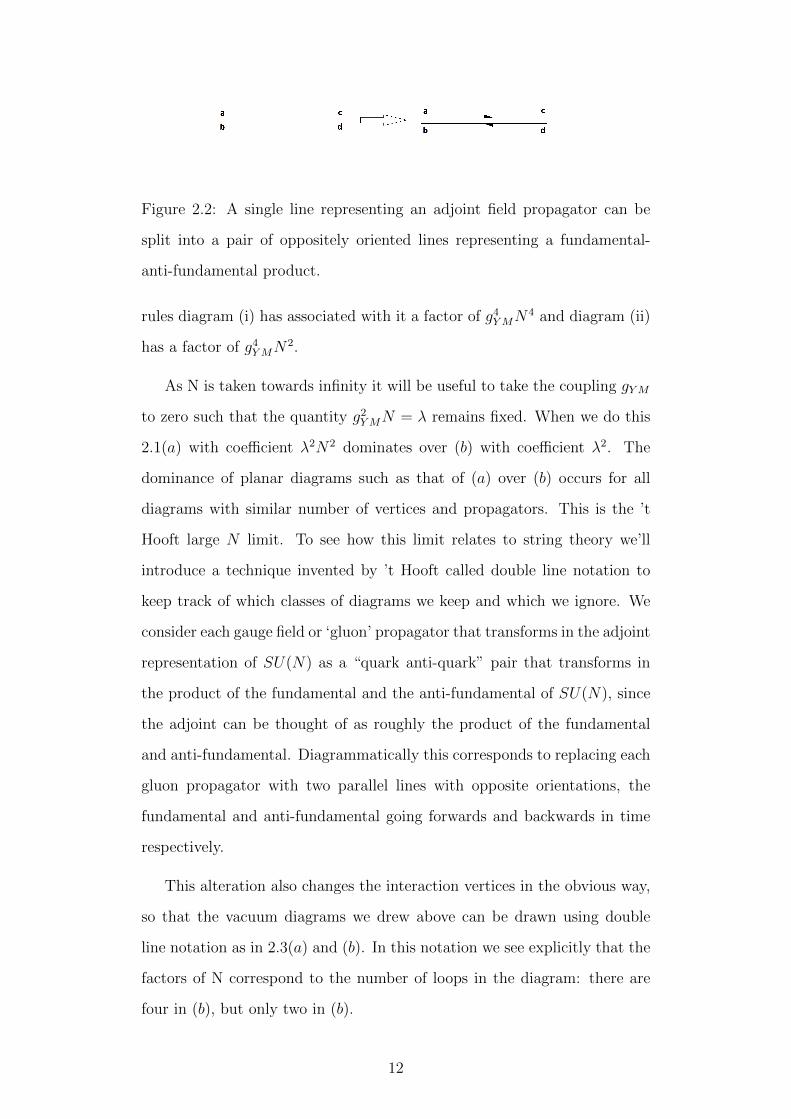
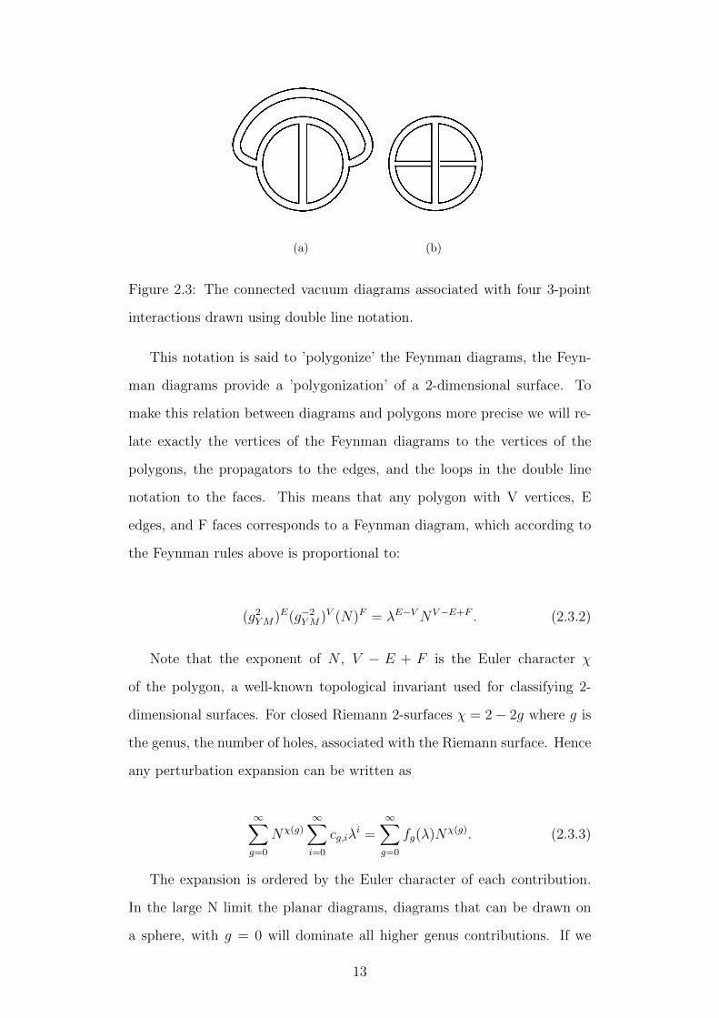


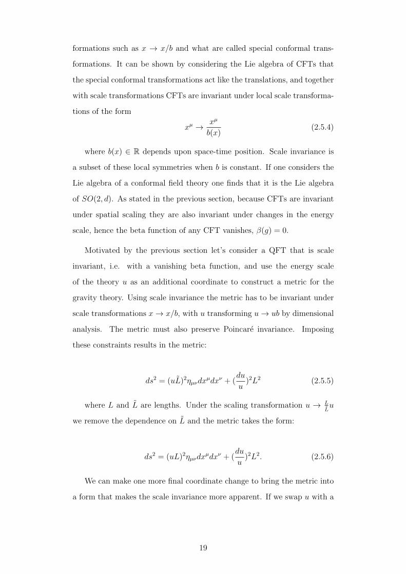


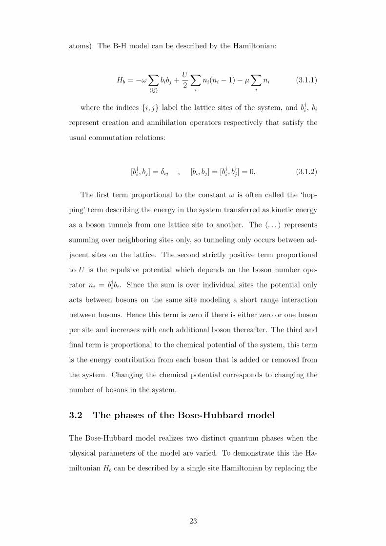

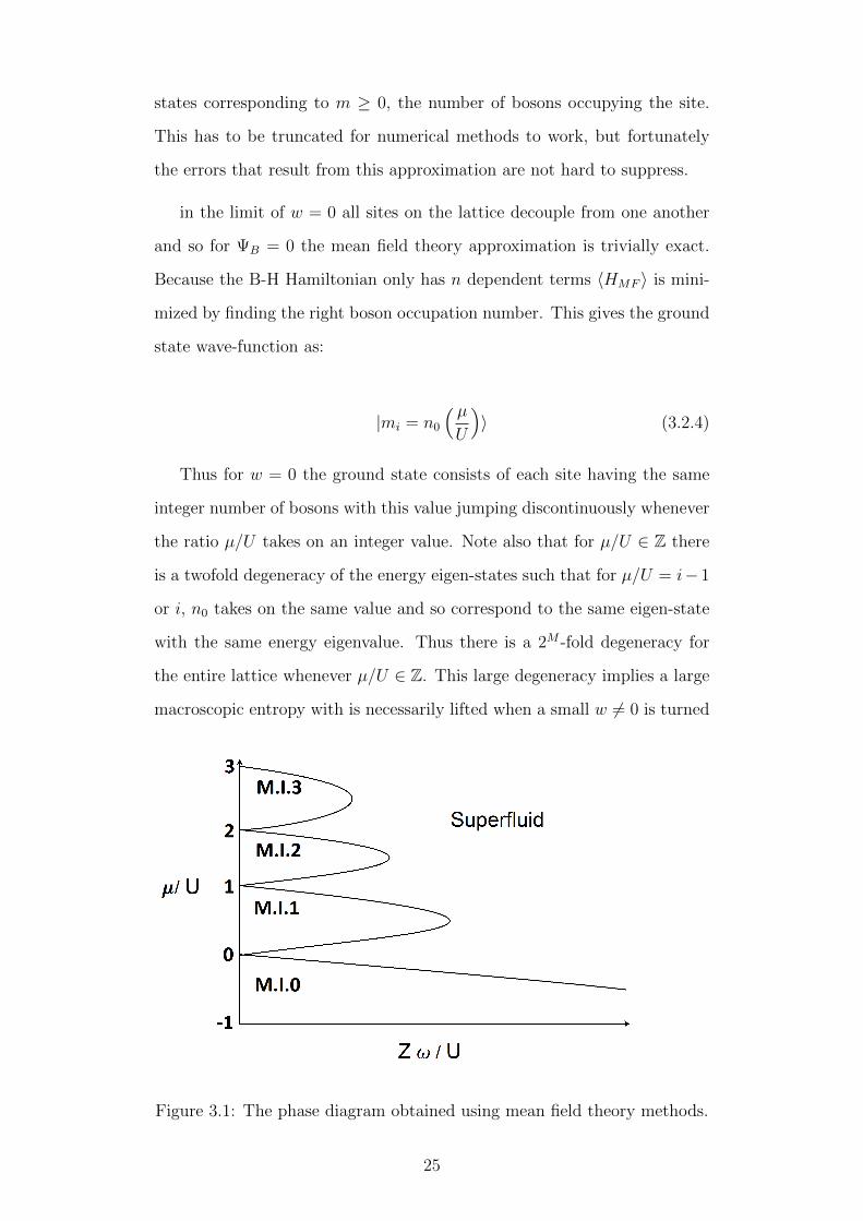

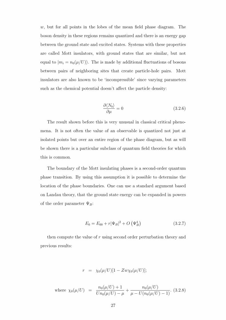
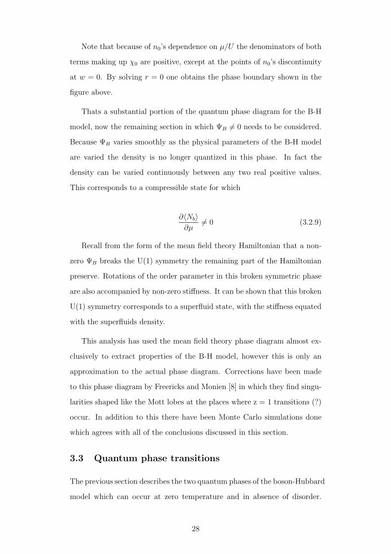


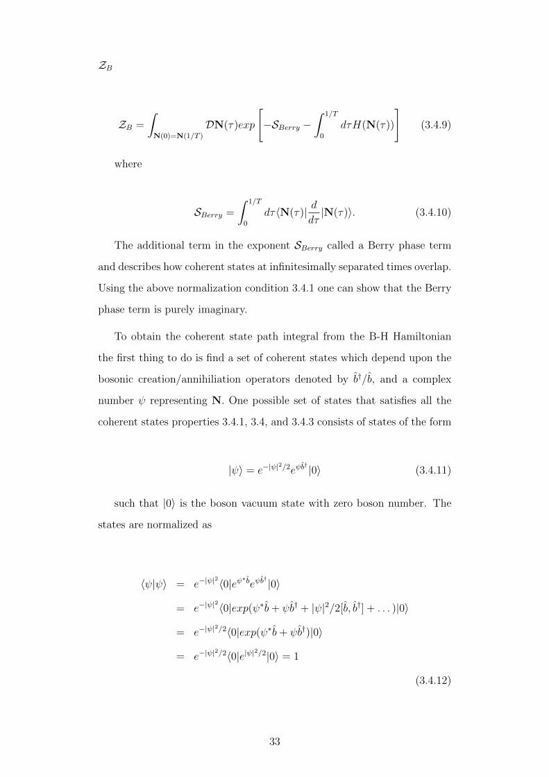
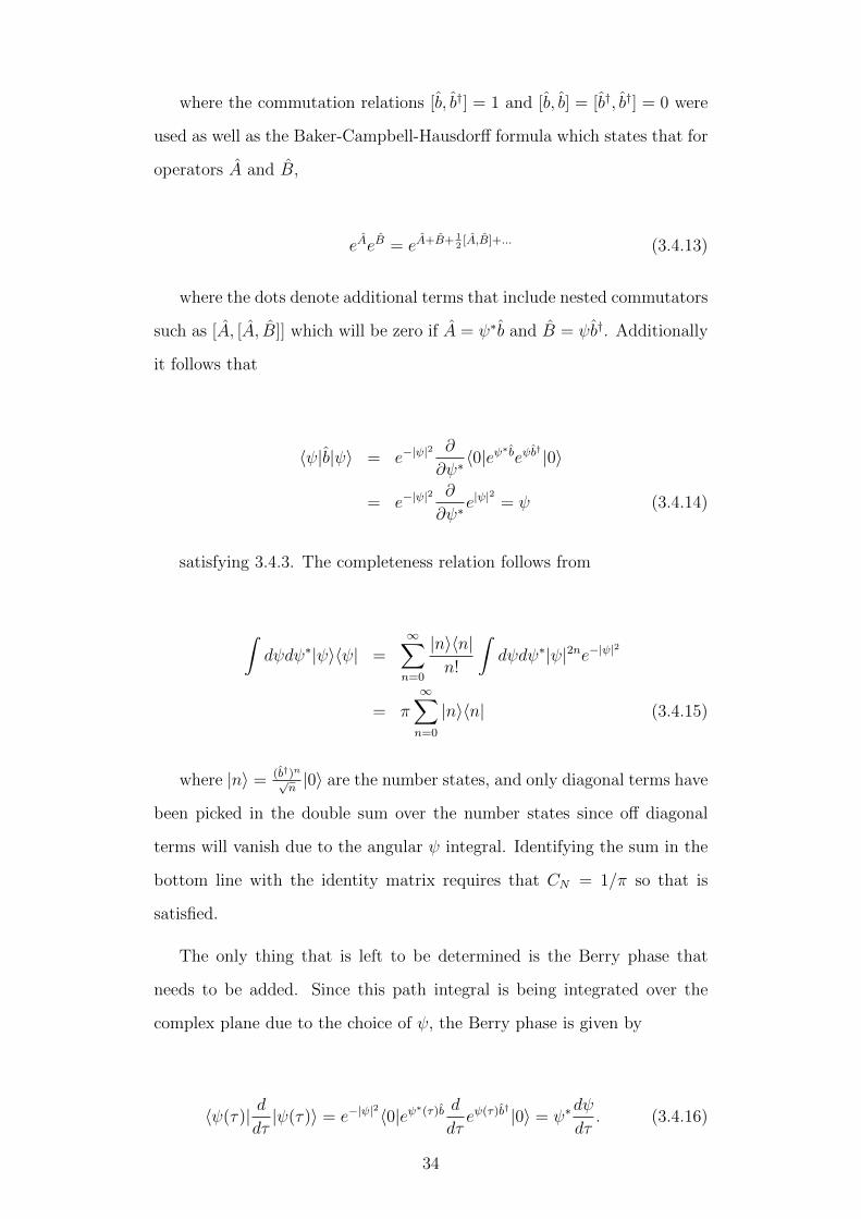


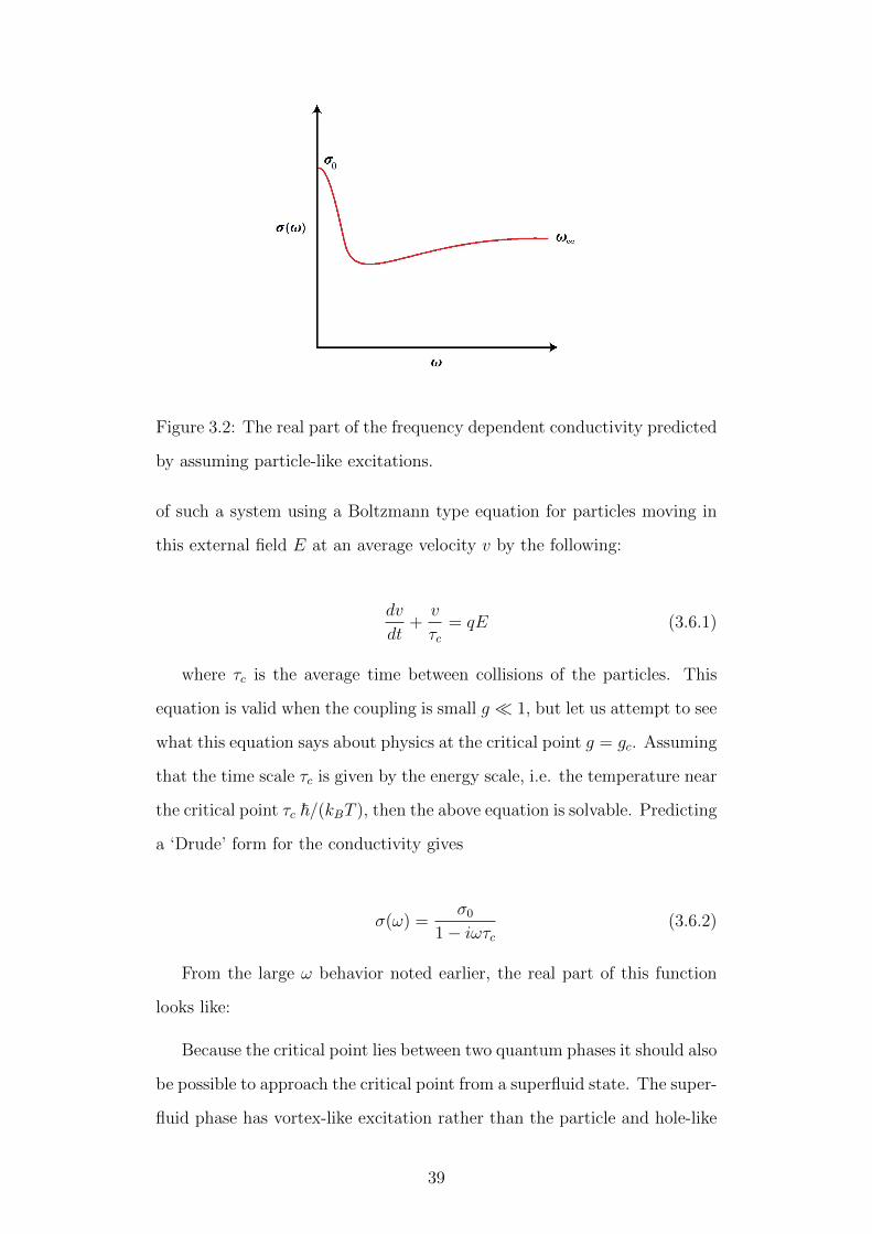


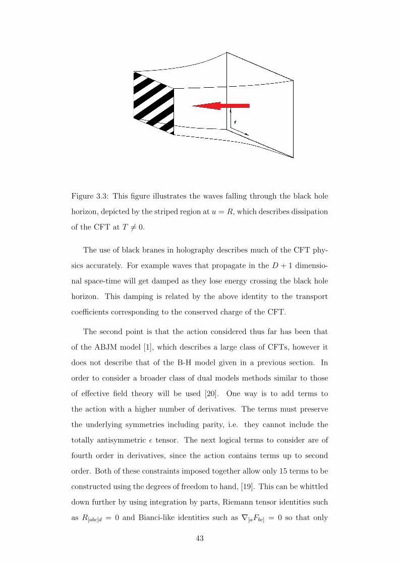


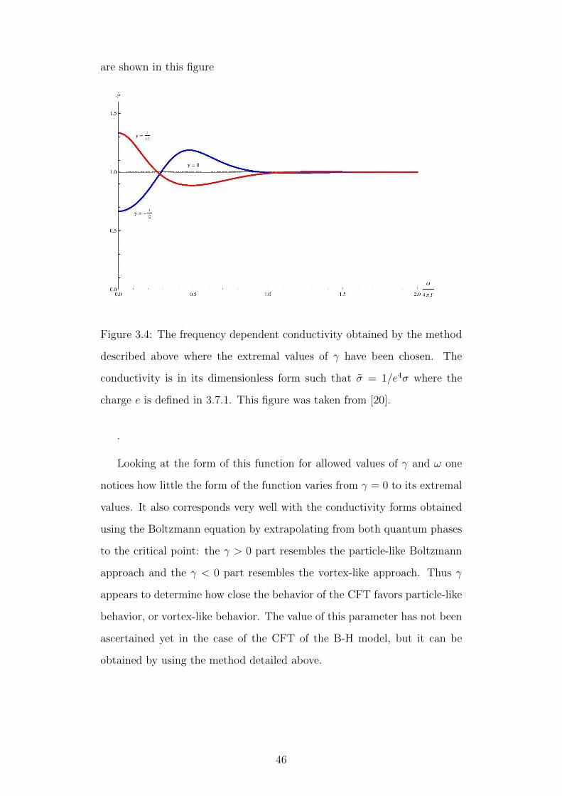


![The AdS/CFT correspondence and condensed matter physics · 2019-12-11 · correspondence [29]. It is a remarkable duality between gravitational sys-tems and ultra-cold atoms, which](https://static.documents.pub/doc/80x56/5f0a99da7e708231d42c6eca/the-adscft-correspondence-and-condensed-matter-physics-2019-12-11-correspondence.jpg)


