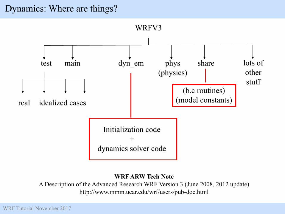
WRF Tutorial November 2017 The Advanced Research WRF (ARW) Dynamics Solver 1. What is a dynamics solver? 2. Variables and coordinates 3. Equations 4. Time integration scheme 5. Grid staggering 6. Advection (transport) and conservation 7. Time step parameters 8. Filters 9. Map projections and global configuration 10. Boundary condition options Dynamics: Introduction WRF ARW Tech Note A Description of the Advanced Research WRF Version 3 (June 2008, 2012 update) http://www.mmm.ucar.edu/wrf/users/pub-doc.html
Transcript
WRF Tutorial November 2017
The Advanced Research WRF(ARW) Dynamics Solver
1. What is a dynamics solver? 2. Variables and coordinates3. Equations 4. Time integration scheme5. Grid staggering6. Advection (transport) and conservation7. Time step parameters8. Filters9. Map projections and global configuration10. Boundary condition options
Dynamics: Introduction
WRF ARW Tech NoteA Description of the Advanced Research WRF Version 3 (June 2008, 2012 update)
http://www.mmm.ucar.edu/wrf/users/pub-doc.html
WRF Tutorial November 2017
Dynamics: 1. What is a dynamics solver?
A dynamical solver (or a dynamical core, or dycore) performs a time (t) and space (x,y,z) integration of the equations of motion.
Given the 3D atmospheric state at time t, S(x,y,z,t), we integrate the equations forward in time from t T, i.e. we run the model and produce a forecast.
The equations cannot be solved analytically, so we discretize the equations on a grid and compute approximate solutions.
The accuracy of the solutions depend on the numerical method and the mesh spacing (grid).
WRF Tutorial November 2017
η=πd −πt( )µd
Dry hydrostatic pressure π
d
Vertical coordinate
Column mass(per unit area)
Layer mass(per unit area)
Dynamics: 2. Variables and coordinates
Vertical coordinates: (1) Traditional terrain-following mass coordinate
π s
π t
πd η( )= ηµd +πt, Pressure
η
µdΔη=Δπd =−gρdΔz
µd = πs−πt
WRF Tutorial November 2017
Dynamics: 2. Variables and coordinates
Vertical coordinates: (2) Hybrid terrain-following mass coordinate
π s
π t
η
cη
Hybrid terrain-following coordinate:
Isobaric coordinate (constant pressure):
πd η( )= B(η)µd+πt+[η−B(η)](π0−πt )
ηc level at which B 0, i.e. transition between isobaric and terrain-following coordinate.
(Terrain-following)
(Isobaric)
η=
πd
π0−πt
WRF Tutorial November 2017
Dynamics: 2. Variables and coordinates
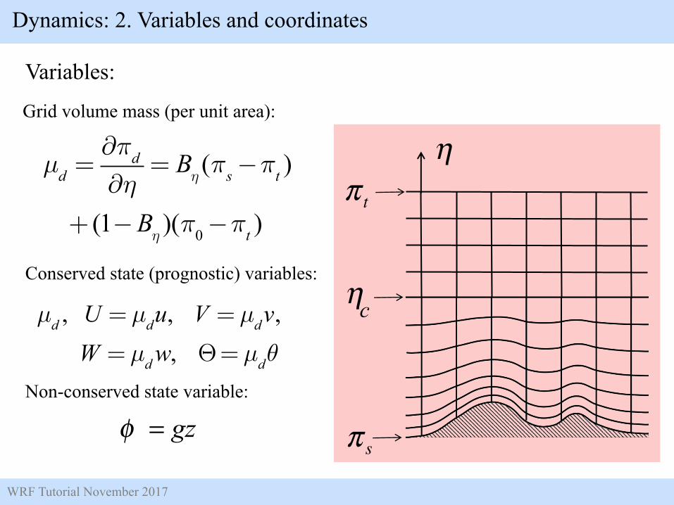
Variables:
π s
π t
η
cη
µd , U = µdu, V = µdv,W = µd w, Θ= µdθ
Conserved state (prognostic) variables:
Non-conserved state variable:
gz=φ
µd =∂πd∂η= Bη (πs−πt )
+ (1−Bη )(π0−πt )
Grid volume mass (per unit area):
WRF Tutorial November 2017
Vertical momentum eqn.
Subscript d denotes dry, and
covariant (u, ω) and contravariant w velocities
Dynamics: 2. Variables and coordinates
u =dxdt
, w =dzdt
, ω=dηdt
U = µu, W = µw, Ω= µω
ααd= 1+qv +qc+qr +⋅⋅⋅( )−1
ρ= ρd 1+ qv + qc + qr + ⋅⋅⋅( )
WRF Tutorial November 2017
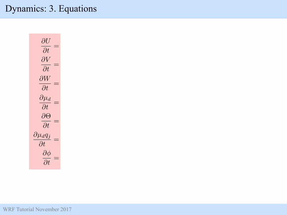
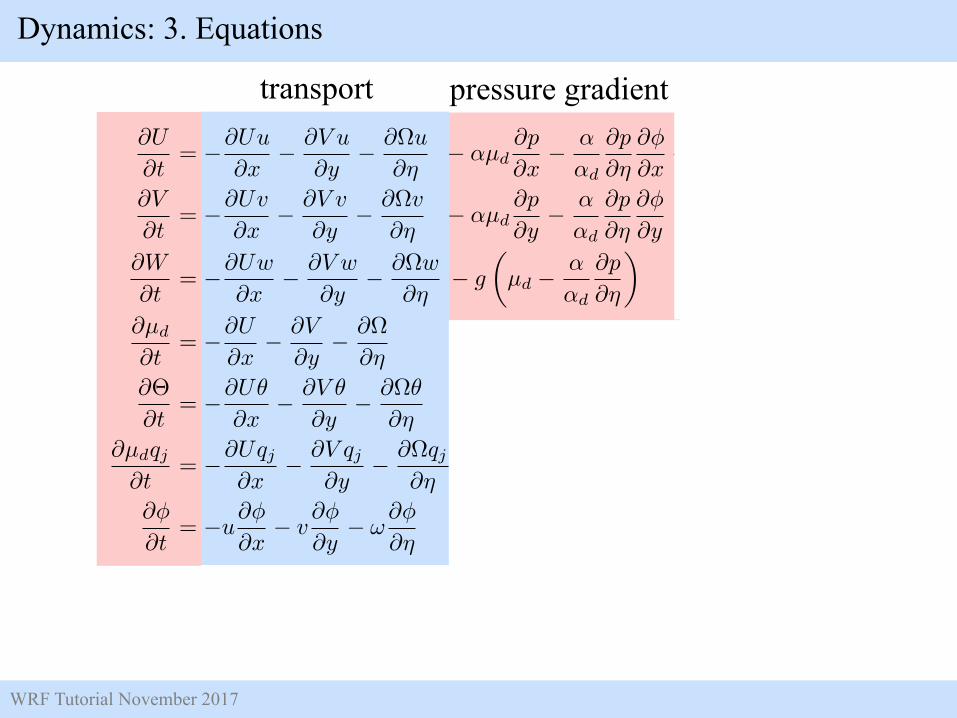
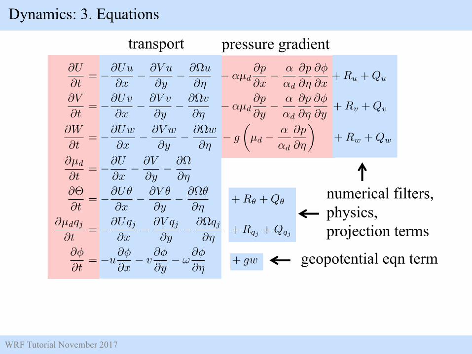
Dynamics: 3. Equations
@U
@t
= �@Uu
@x
� @V u
@y
� @⌦u
@⌘
� ↵µ
d
@p
@x
� ↵
↵
d
@p
@⌘
@�
@x
+R
u
+Q
u
@V
@t
= �@Uv
@x
� @V v
@y
� @⌦v
@⌘
� ↵µ
d
@p
@y
� ↵
↵
d
@p
@⌘
@�
@y
+R
v
+Q
v
@W
@t
= �@Uw
@x
� @V w
@y
� @⌦w
@⌘
� g
✓µ
d
� ↵
↵
d
@p
@⌘
◆+R
w
+Q
w
@µ
d
@t
= �@U
@x
� @V
@y
� @⌦
@⌘
@⇥
@t
= �@U✓
@x
� @V ✓
@y
� @⌦✓
@⌘
+R
✓
+Q
✓
@µ
d
q
j
@t
= �@Uq
j
@x
� @V q
j
@y
� @⌦qj
@⌘
+R
qj +Q
qj
@�
@t
= �u
@�
@x
� v
@�
@y
� !
@�
@⌘
+ gw
3
WRF Tutorial November 2017
Dynamics: 3. Equations
@U
@t
= �@Uu
@x
� @V u
@y
� @⌦u
@⌘
� ↵µ
d
@p
@x
� ↵
↵
d
@p
@⌘
@�
@x
+R
u
+Q
u
@V
@t
= �@Uv
@x
� @V v
@y
� @⌦v
@⌘
� ↵µ
d
@p
@y
� ↵
↵
d
@p
@⌘
@�
@y
+R
v
+Q
v
@W
@t
= �@Uw
@x
� @V w
@y
� @⌦w
@⌘
� g
✓µ
d
� ↵
↵
d
@p
@⌘
◆+R
w
+Q
w
@µ
d
@t
= �@U
@x
� @V
@y
� @⌦
@⌘
@⇥
@t
= �@U✓
@x
� @V ✓
@y
� @⌦✓
@⌘
+R
✓
+Q
✓
@µ
d
q
j
@t
= �@Uq
j
@x
� @V q
j
@y
� @⌦qj
@⌘
+R
qj +Q
qj
@�
@t
= �u
@�
@x
� v
@�
@y
� !
@�
@⌘
+ gw
3
transport
WRF Tutorial November 2017
Dynamics: 3. Equations
@U
@t
= �@Uu
@x
� @V u
@y
� @⌦u
@⌘
� ↵µ
d
@p
@x
� ↵
↵
d
@p
@⌘
@�
@x
+R
u
+Q
u
@V
@t
= �@Uv
@x
� @V v
@y
� @⌦v
@⌘
� ↵µ
d
@p
@y
� ↵
↵
d
@p
@⌘
@�
@y
+R
v
+Q
v
@W
@t
= �@Uw
@x
� @V w
@y
� @⌦w
@⌘
� g
✓µ
d
� ↵
↵
d
@p
@⌘
◆+R
w
+Q
w
@µ
d
@t
= �@U
@x
� @V
@y
� @⌦
@⌘
@⇥
@t
= �@U✓
@x
� @V ✓
@y
� @⌦✓
@⌘
+R
✓
+Q
✓
@µ
d
q
j
@t
= �@Uq
j
@x
� @V q
j
@y
� @⌦qj
@⌘
+R
qj +Q
qj
@�
@t
= �u
@�
@x
� v
@�
@y
� !
@�
@⌘
+ gw
3
transport pressure gradient
numerical filters, physics, projection terms
geopotential eqn term
WRF Tutorial November 2017
Diagnostic relations:
Dynamics: 3. Equations
p = RdΘm
poµdα d
⎛⎝⎜
⎞⎠⎟
γ
, Θm =Θ 1+ RvRdqv
⎛⎝⎜
⎞⎠⎟
@U
@t
= �@Uu
@x
� @V u
@y
� @⌦u
@⌘
� ↵µ
d
@p
@x
� ↵
↵
d
@p
@⌘
@�
@x
+R
u
+Q
u
@V
@t
= �@Uv
@x
� @V v
@y
� @⌦v
@⌘
� ↵µ
d
@p
@y
� ↵
↵
d
@p
@⌘
@�
@y
+R
v
+Q
v
@W
@t
= �@Uw
@x
� @V w
@y
� @⌦w
@⌘
� g
✓µ
d
� ↵
↵
d
@p
@⌘
◆+R
w
+Q
w
@µ
d
@t
= �@U
@x
� @V
@y
� @⌦
@⌘
@⇥
@t
= �@U✓
@x
� @V ✓
@y
� @⌦✓
@⌘
+R
✓
+Q
✓
@µ
d
q
j
@t
= �@Uq
j
@x
� @V q
j
@y
� @⌦qj
@⌘
+R
qj +Q
qj
@�
@t
= �u
@�
@x
� v
@�
@y
� !
@�
@⌘
+ gw
3
transport pressure gradient
numerical filters, physics, projection terms
geopotential eqn. term
WRF Tutorial November 2017
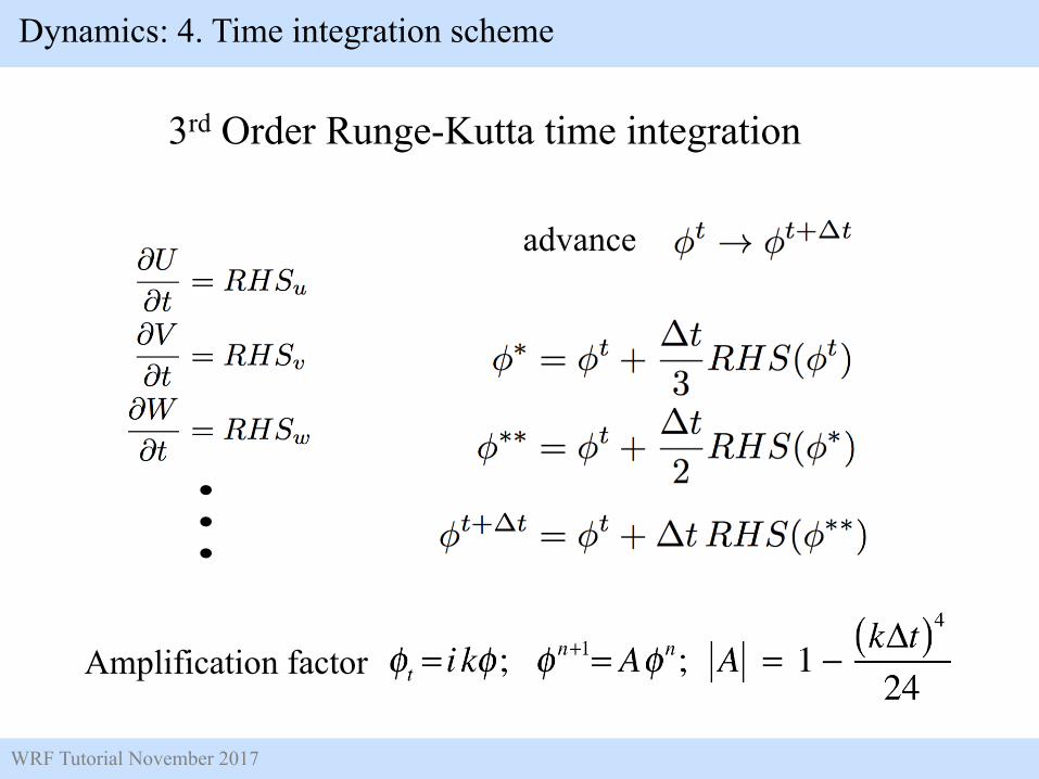
3rd Order Runge-Kutta time integration
Amplification factor
advance
Dynamics: 4. Time integration scheme
WRF Tutorial November 2017
t t+dtt+dt/3
t t+dtt+dt/2
t t+dt
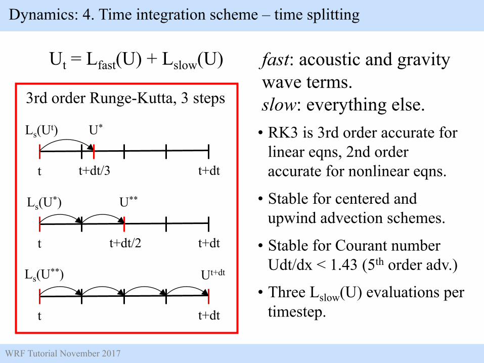
Ut = Lfast(U) + Lslow(U)
Ls(Ut) U*
Ls(U*) U**
Ls(U**) Ut+dt
3rd order Runge-Kutta, 3 steps
• RK3 is 3rd order accurate for linear eqns, 2nd order accurate for nonlinear eqns.
• Stable for centered and upwind advection schemes.
• Stable for Courant number Udt/dx < 1.43 (5th order adv.)
• Three Lslow(U) evaluations per timestep.
Dynamics: 4. Time integration scheme – time splitting
fast: acoustic and gravity wave terms.slow: everything else.
WRF Tutorial November 2017
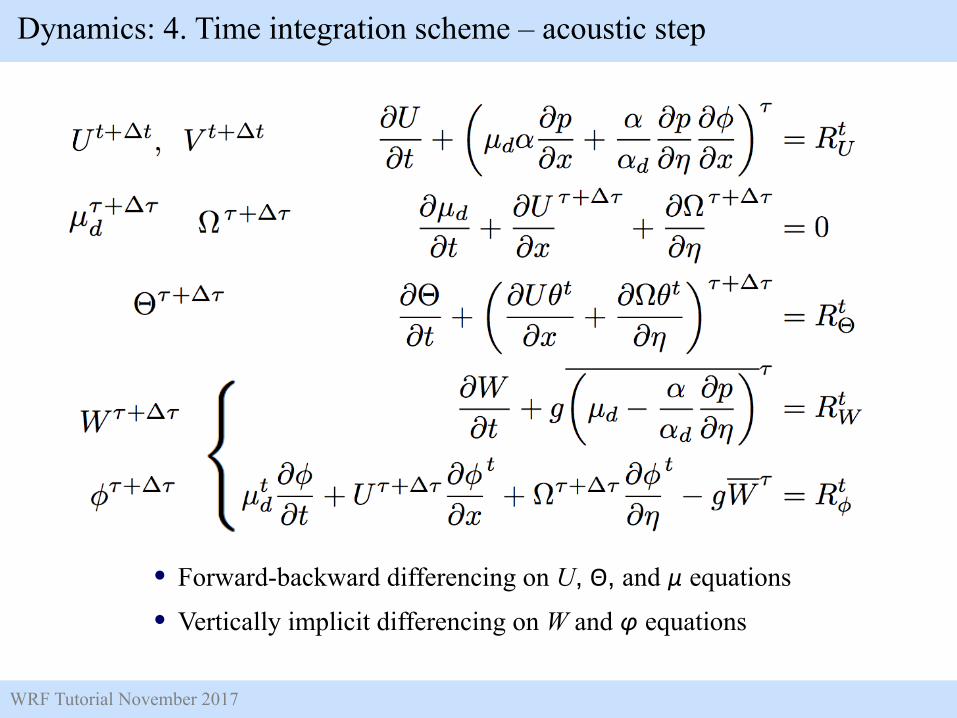
• Forward-backward differencing on U, Θ, and μ equations
• Vertically implicit differencing on W and φ equations
Dynamics: 4. Time integration scheme – acoustic step
WRF Tutorial November 2017
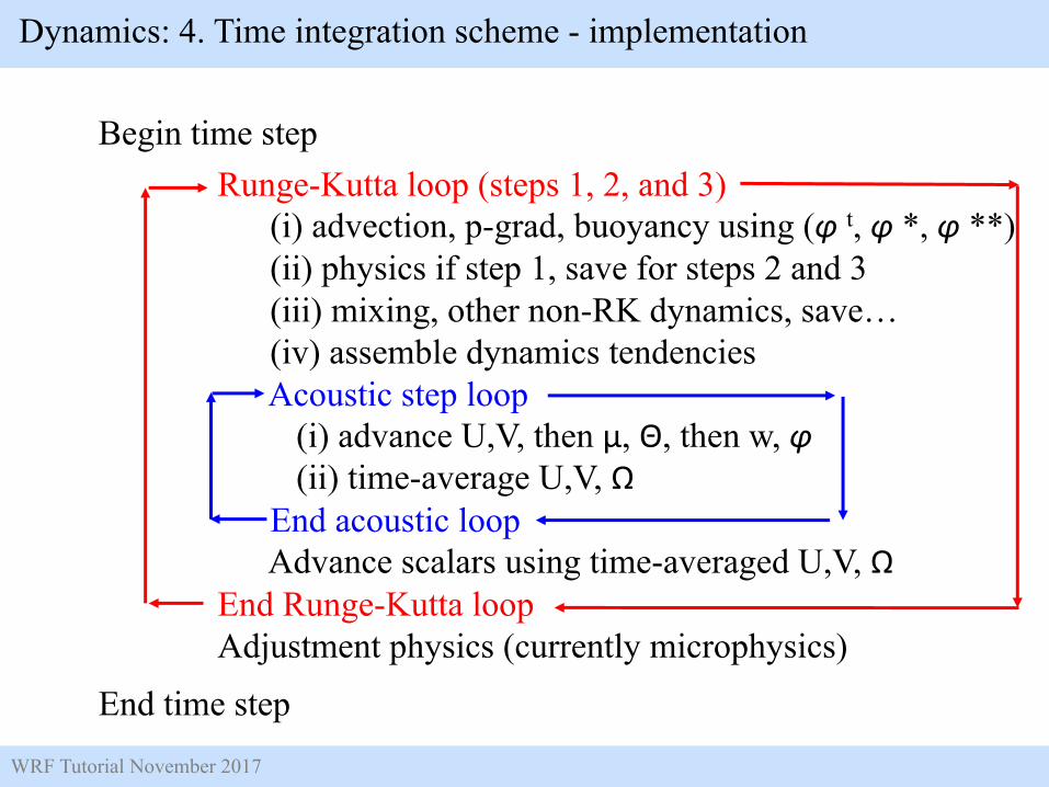
Runge-Kutta loop (steps 1, 2, and 3)(i) advection, p-grad, buoyancy using (φ t, φ *, φ **) (ii) physics if step 1, save for steps 2 and 3(iii) mixing, other non-RK dynamics, save…(iv) assemble dynamics tendenciesAcoustic step loop
(i) advance U,V, then μ, Θ, then w, φ(ii) time-average U,V, Ω
End acoustic loopAdvance scalars using time-averaged U,V, Ω
End Runge-Kutta loopAdjustment physics (currently microphysics)
Begin time step
End time step
Dynamics: 4. Time integration scheme - implementation
WRF Tutorial November 2017
h
Ω,W, φ
U U
x�
µ,θ,qv,ql
V
V
U U
x
y
�
µ,θ,qv,ql
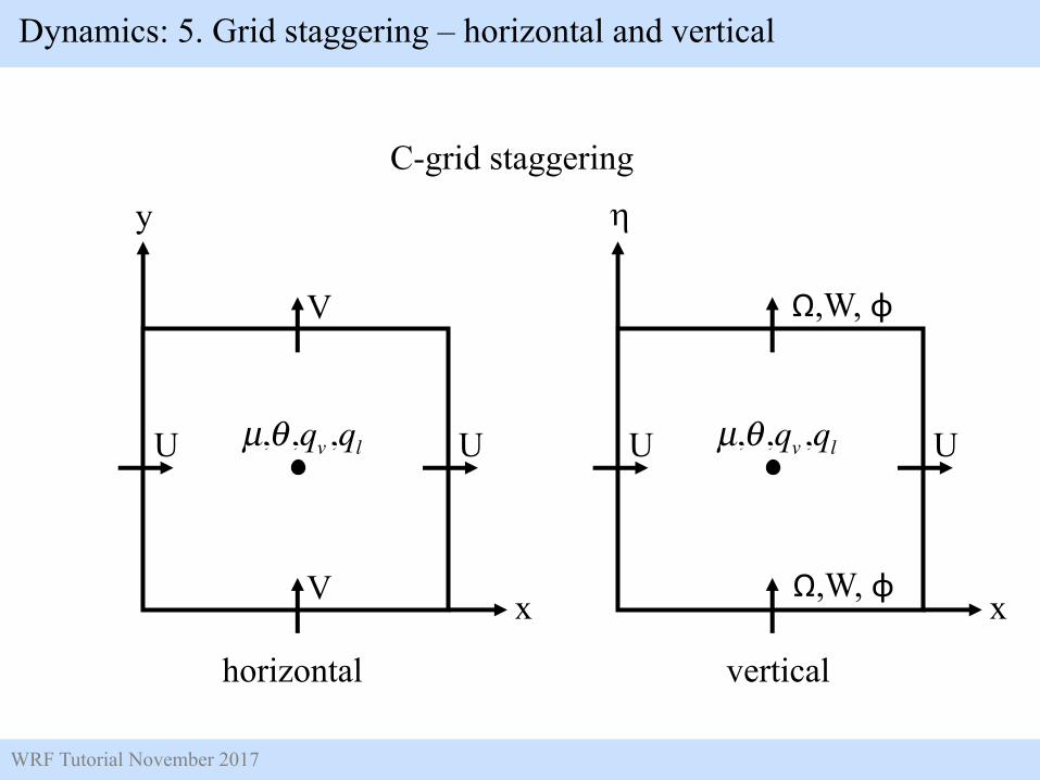
C-grid staggering
horizontal vertical
Ω,W, φ
Dynamics: 5. Grid staggering – horizontal and vertical
WRF Tutorial November 2017
Diagnostic relations: p = RdΘm
poµdα d
⎛⎝⎜
⎞⎠⎟
γ
, Θm =Θ 1+ RvRdqv
⎛⎝⎜
⎞⎠⎟
@U
@t
= �@Uu
@x
� @V u
@y
� @⌦u
@⌘
� ↵µ
d
@p
@x
� ↵
↵
d
@p
@⌘
@�
@x
+R
u
+Q
u
@V
@t
= �@Uv
@x
� @V v
@y
� @⌦v
@⌘
� ↵µ
d
@p
@y
� ↵
↵
d
@p
@⌘
@�
@y
+R
v
+Q
v
@W
@t
= �@Uw
@x
� @V w
@y
� @⌦w
@⌘
� g
✓µ
d
� ↵
↵
d
@p
@⌘
◆+R
w
+Q
w
@µ
d
@t
= �@U
@x
� @V
@y
� @⌦
@⌘
@⇥
@t
= �@U✓
@x
� @V ✓
@y
� @⌦✓
@⌘
+R
✓
+Q
✓
@µ
d
q
j
@t
= �@Uq
j
@x
� @V q
j
@y
� @⌦qj
@⌘
+R
qj +Q
qj
@�
@t
= �u
@�
@x
� v
@�
@y
� !
@�
@⌘
+ gw
3
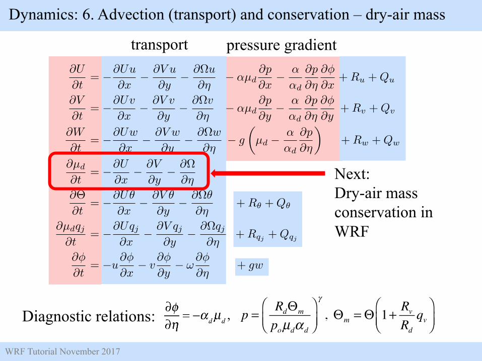
transport pressure gradient
Next:Dry-air mass conservation in WRF
Dynamics: 6. Advection (transport) and conservation – dry-air mass
WRF Tutorial November 2017
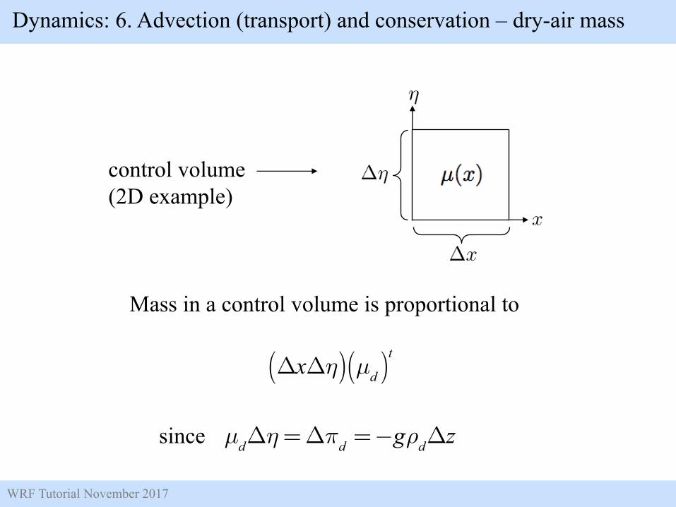
control volume(2D example)
Mass in a control volume is proportional to
since
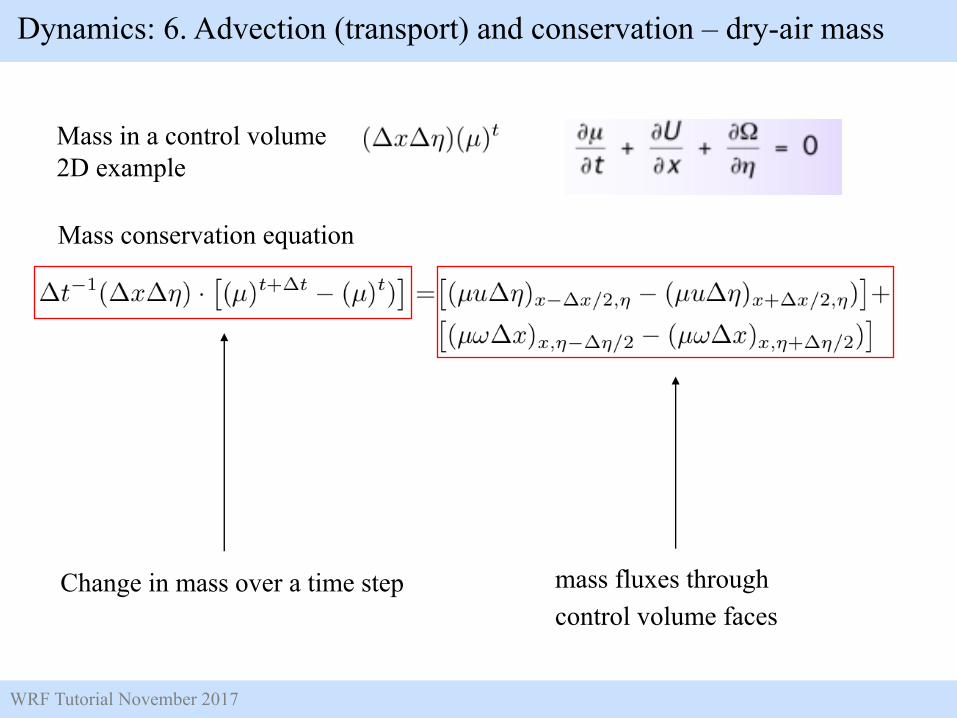
Dynamics: 6. Advection (transport) and conservation – dry-air mass
ΔxΔη( ) µd( )t
µdΔη=Δπd =−gρdΔz
WRF Tutorial November 2017
Mass in a control volume2D example
Mass conservation equation
Change in mass over a time step mass fluxes through control volume faces
Dynamics: 6. Advection (transport) and conservation – dry-air mass
WRF Tutorial November 2017
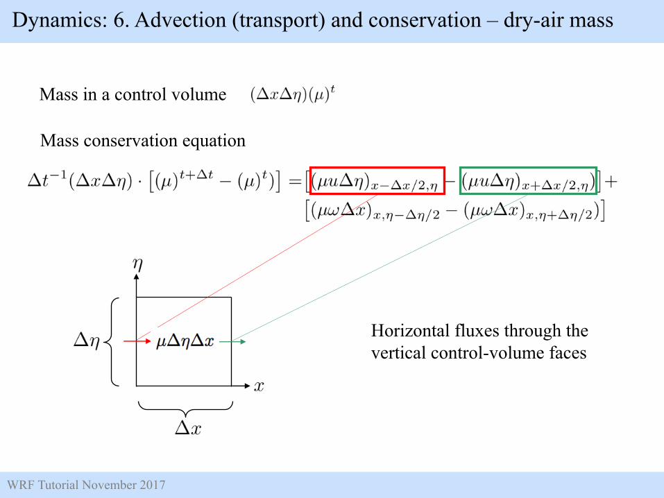
Mass in a control volume
Mass conservation equation
Horizontal fluxes through the vertical control-volume faces
Dynamics: 6. Advection (transport) and conservation – dry-air mass
WRF Tutorial November 2017
Mass in a control volume
Mass conservation equation
Vertical fluxes through the horizontal control-volume faces
Dynamics: 6. Advection (transport) and conservation – dry-air mass
WRF Tutorial November 2017
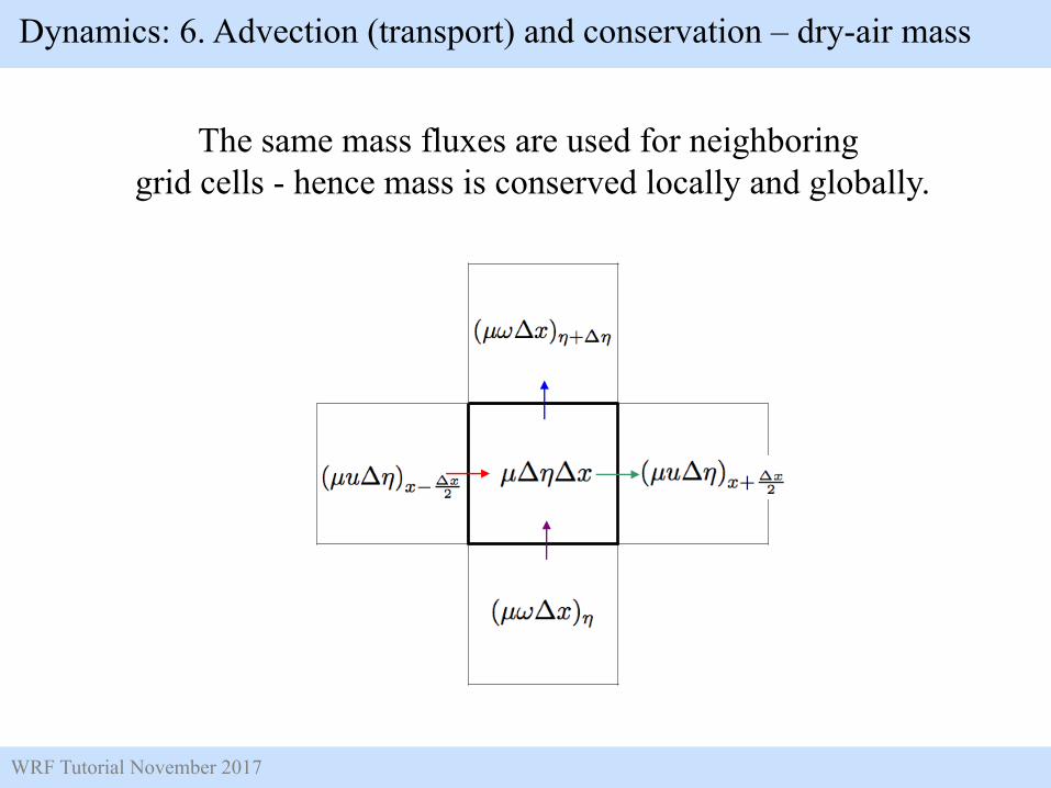
The same mass fluxes are used for neighboring grid cells - hence mass is conserved locally and globally.
Dynamics: 6. Advection (transport) and conservation – dry-air mass
WRF Tutorial November 2017
Diagnostic relations: p = RdΘm
poµdα d
⎛⎝⎜
⎞⎠⎟
γ
, Θm =Θ 1+ RvRdqv
⎛⎝⎜
⎞⎠⎟
@U
@t
= �@Uu
@x
� @V u
@y
� @⌦u
@⌘
� ↵µ
d
@p
@x
� ↵
↵
d
@p
@⌘
@�
@x
+R
u
+Q
u
@V
@t
= �@Uv
@x
� @V v
@y
� @⌦v
@⌘
� ↵µ
d
@p
@y
� ↵
↵
d
@p
@⌘
@�
@y
+R
v
+Q
v
@W
@t
= �@Uw
@x
� @V w
@y
� @⌦w
@⌘
� g
✓µ
d
� ↵
↵
d
@p
@⌘
◆+R
w
+Q
w
@µ
d
@t
= �@U
@x
� @V
@y
� @⌦
@⌘
@⇥
@t
= �@U✓
@x
� @V ✓
@y
� @⌦✓
@⌘
+R
✓
+Q
✓
@µ
d
q
j
@t
= �@Uq
j
@x
� @V q
j
@y
� @⌦qj
@⌘
+R
qj +Q
qj
@�
@t
= �u
@�
@x
� v
@�
@y
� !
@�
@⌘
+ gw
3
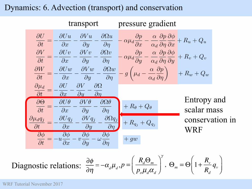
transport pressure gradient
Entropy and scalar mass conservation in WRF
Dynamics: 6. Advection (transport) and conservation
WRF Tutorial November 2017
Mass in a control volume
Mass conservation equation:
change in mass over a time step mass fluxes through control volume faces
Scalar mass
change in tracer mass over a time step
tracer mass fluxes through control volume faces
Scalar mass conservation equation:
Dynamics: 6. Advection (transport) and conservation – scalars
WRF Tutorial November 2017
Diagnostic relations: p = RdΘm
poµdα d
⎛⎝⎜
⎞⎠⎟
γ
, Θm =Θ 1+ RvRdqv
⎛⎝⎜
⎞⎠⎟
@U
@t
= �@Uu
@x
� @V u
@y
� @⌦u
@⌘
� ↵µ
d
@p
@x
� ↵
↵
d
@p
@⌘
@�
@x
+R
u
+Q
u
@V
@t
= �@Uv
@x
� @V v
@y
� @⌦v
@⌘
� ↵µ
d
@p
@y
� ↵
↵
d
@p
@⌘
@�
@y
+R
v
+Q
v
@W
@t
= �@Uw
@x
� @V w
@y
� @⌦w
@⌘
� g
✓µ
d
� ↵
↵
d
@p
@⌘
◆+R
w
+Q
w
@µ
d
@t
= �@U
@x
� @V
@y
� @⌦
@⌘
@⇥
@t
= �@U✓
@x
� @V ✓
@y
� @⌦✓
@⌘
+R
✓
+Q
✓
@µ
d
q
j
@t
= �@Uq
j
@x
� @V q
j
@y
� @⌦qj
@⌘
+R
qj +Q
qj
@�
@t
= �u
@�
@x
� v
@�
@y
� !
@�
@⌘
+ gw
3
transport pressure gradient
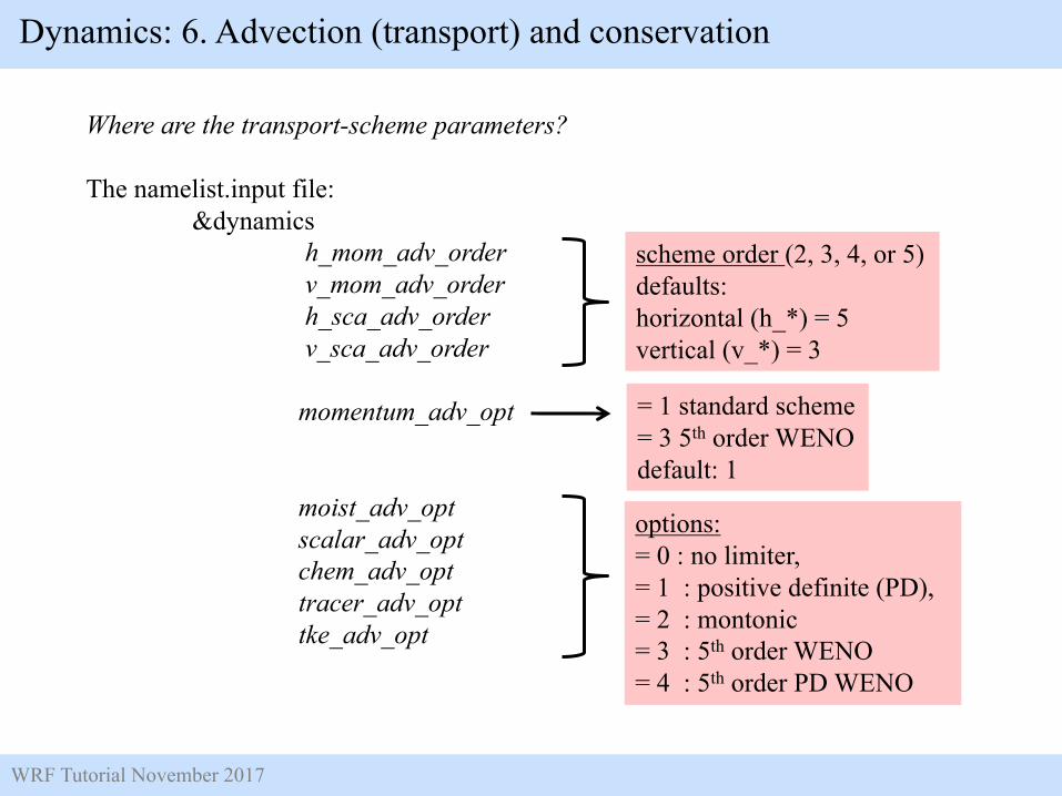
Transport schemes: flux divergence (transport) options in WRF
Dynamics: 6. Advection (transport) and conservation
WRF Tutorial November 2017
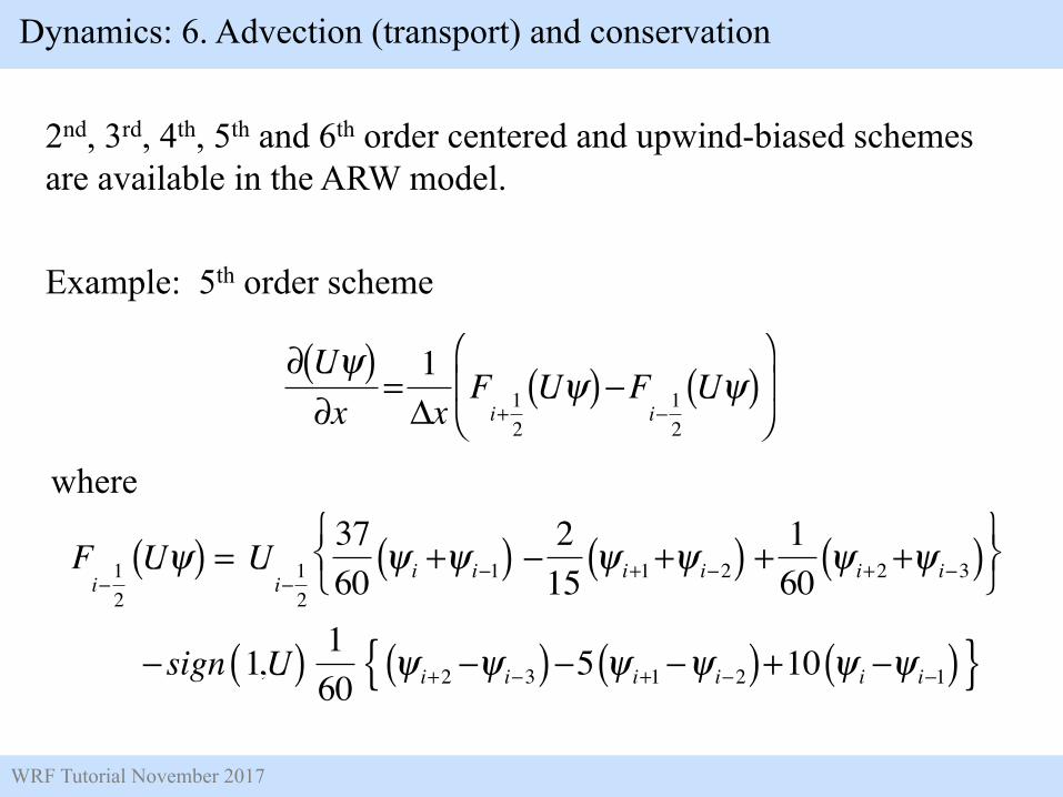
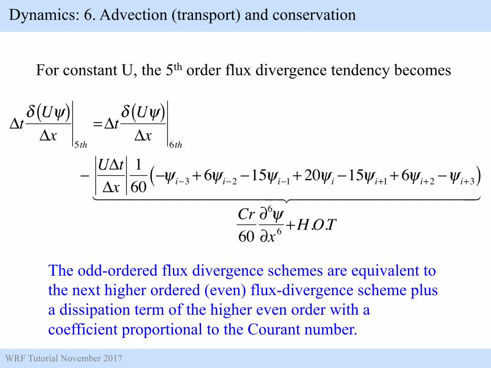
2nd, 3rd, 4th, 5th and 6th order centered and upwind-biased schemesare available in the ARW model.
The odd-ordered flux divergence schemes are equivalent to the next higher ordered (even) flux-divergence scheme plus a dissipation term of the higher even order with a coefficient proportional to the Courant number.
Dynamics: 6. Advection (transport) and conservation
WRF Tutorial November 2017
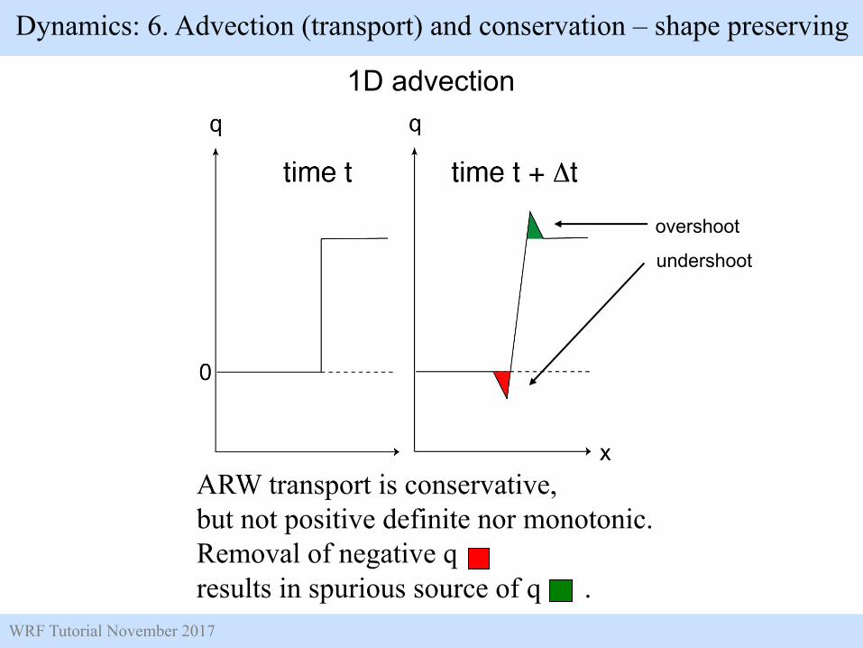
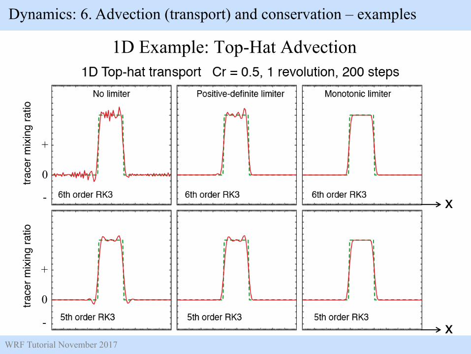
ARW transport is conservative, but not positive definite nor monotonic.Removal of negative qresults in spurious source of q .
1D advection
overshoot
undershoot
Dynamics: 6. Advection (transport) and conservation – shape preserving
WRF Tutorial November 2017
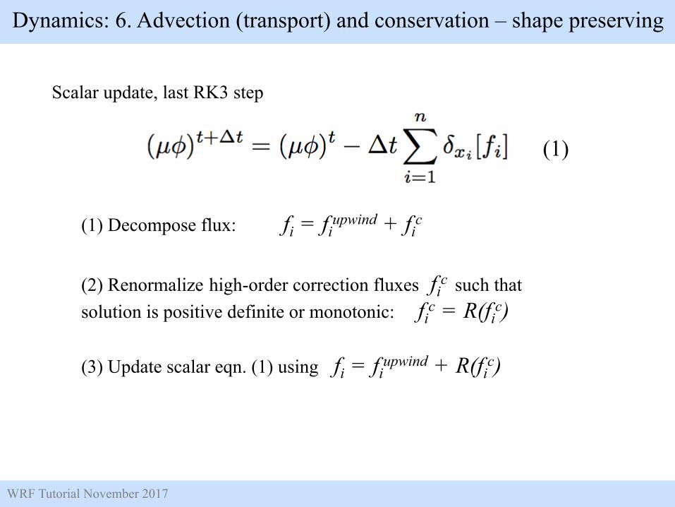
(1) Decompose flux: fi = fiupwind + fi
c
(3) Update scalar eqn. (1) using fi = fiupwind + R(fi
c)
Scalar update, last RK3 step
(2) Renormalize high-order correction fluxes fic such that
solution is positive definite or monotonic: fic = R(fi
c)
(1)
Dynamics: 6. Advection (transport) and conservation – shape preserving
WRF Tutorial November 2017
1D Example: Top-Hat Advection
Dynamics: 6. Advection (transport) and conservation – examples
0
0
trace
r mix
ing
ratio
trace
r mix
ing
ratio
+
+
-
-
x
x
WRF Tutorial November 2017
Dynamics: 6. Advection (transport) and conservation
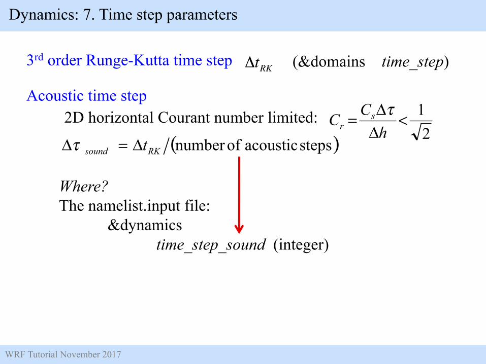
Acoustic time step2D horizontal Courant number limited:
21<
ΔΔ=h
CC sr
τ
( )stepsacousticofnumberRKsound tΔ=Δτ
Dynamics: 7. Time step parameters
€
ΔtRK (&domains time_step)
Where?The namelist.input file:
&dynamicstime_step_sound (integer)
WRF Tutorial November 2017
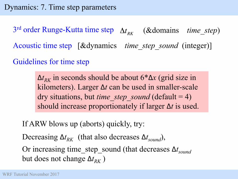
3rd order Runge-Kutta time step
Acoustic time step
Dynamics: 7. Time step parameters
€
ΔtRK (&domains time_step)
[&dynamics time_step_sound (integer)]
ΔtRK in seconds should be about 6*Δx (grid size in kilometers). Larger Δt can be used in smaller-scale dry situations, but time_step_sound (default = 4) should increase proportionately if larger Δt is used.
Guidelines for time step
Decreasing ΔtRK (that also decreases Δtsound),Or increasing time_step_sound (that decreases Δtsoundbut does not change ΔtRK )
If ARW blows up (aborts) quickly, try:
WRF Tutorial November 2017
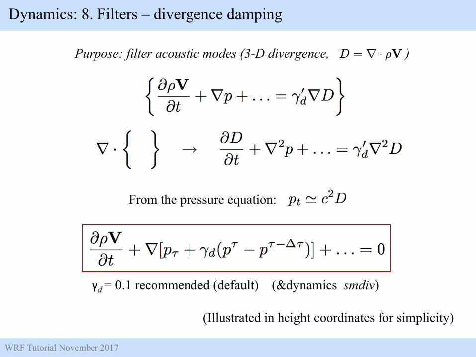
Purpose: filter acoustic modes (3-D divergence, )
From the pressure equation:
(Illustrated in height coordinates for simplicity)
Projections 1-4 are isotropic (mx = my)Latitude-longitude projection is anistropic (mx ≠ my)
Dynamics: 9. Map projections and global configuration
WRF Tutorial November 2017
Converging gridlines severely limit timestep.The polar filter removes this limitation.
Filter procedure - Along a grid latitude circle:1. Fourier transform variable.2. Filter Fourier coefficients.3. Transform back to physical space.
Dynamics: 9. Map projections and global configuration
Global ARW – Polar filters
WRF Tutorial November 2017
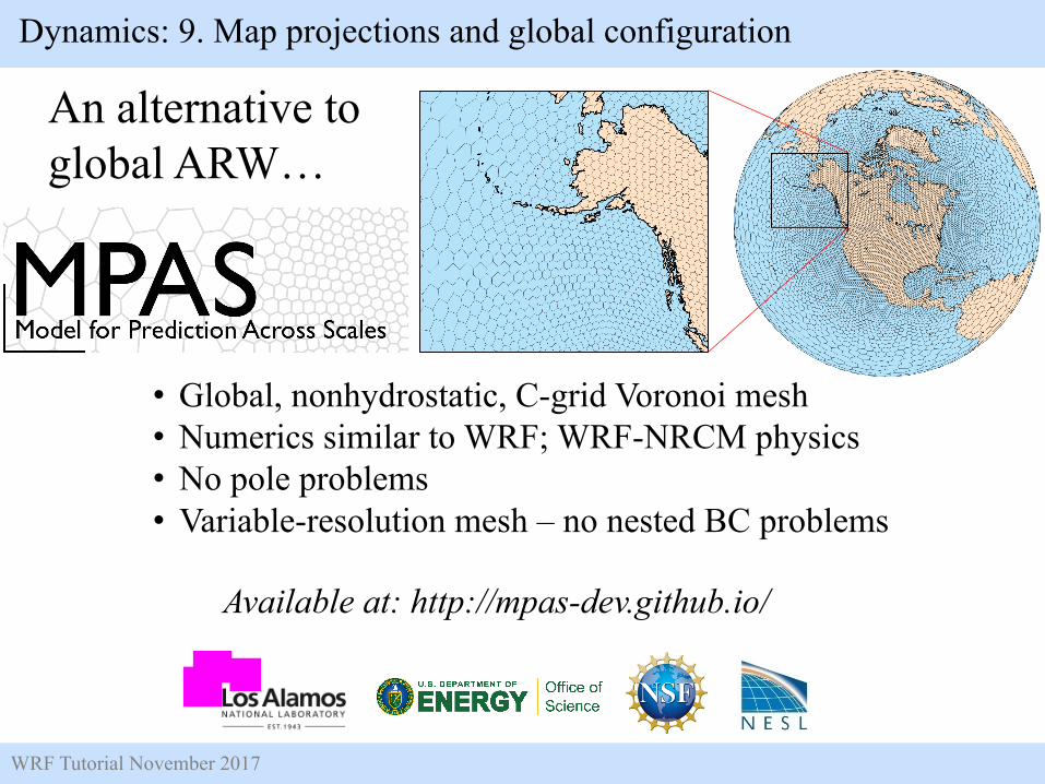
An alternative to global ARW…
• Global, nonhydrostatic, C-grid Voronoi mesh• Numerics similar to WRF; WRF-NRCM physics• No pole problems• Variable-resolution mesh – no nested BC problems
Available at: http://mpas-dev.github.io/
Dynamics: 9. Map projections and global configuration