The advantage and disadvantage of implicitly stratified sampling Peter Lynn Institute for Social and Economic Research University of Essex Understanding Society Working Paper Series No. 2016 – 05 August 2016
Transcript
The advantage and disadvantage of implicitly stratified sampling
Peter Lynn
Institute for Social and Economic Research
University of Essex
Understanding Society
Working Paper Series
No. 2016 – 05
August 2016
The advantage and disadvantage of implicitly strati fied sampling
Peter Lynn
Non-Technical Summary
The statistical precision of estimates from sample-based surveys is influenced by the
way the sample of persons to be interviewed is selected. “Proportionate stratified
sampling” is a technique used to ensure that the sample profile matches that of the
population from which the sample is selected in some respects. The better the match
between the sample profile and the population profile, the more precise the estimates
will be. However, there are many different ways to implement proportionate stratified
sampling and a key distinction is between “implicit” and “explicit” proportionate stratified
sampling. Implicit stratified sampling would involve, for example, listing all the people in
the population in order of date of birth and then sampling every 100th person on the list.
Explicit stratified sampling, on the other hand, might involve sorting people into a
number of age groups and then randomly sampling 1 in 100 people from each age
group in turn.
In this paper we compare these two methods of sample selection. We do this by
pretending that the Understanding Society wave 1 sample of respondents is in fact a
complete population that we wish to study. Because we know the survey responses of
everyone in the population, we can calculate exactly how precise estimates would be
with each method of selecting a sample from this population. In this way, we can show
how much more precise the implicit method is than the explicit method.
However, one drawback of the implicit method in a real survey situation (when we do
not know how all the other population members – not selected into the survey sample –
would have answered the survey questions) is that it is not possible to estimate well
how precise the survey estimates are. Instead, an approximation is used that tends to
under-estimate the precision. Because in this study we know the true precision of the
estimates that would be obtained with implicit stratified sampling, we are able to show
by how much this precision is under-estimated.
In conclusion, the paper argues that implicit proportionate stratified sampling may be
preferable to explicit proportionate stratified sampling as it provides better precision,
even though survey users may not have good information about how much more
precise the estimates are.
The advantage and disadvantage of implicitly strati fied sampling
Peter Lynn
Abstract
Explicit stratified sampling (ESS) and implicit stratified sampling (ISS) are alternative
methods for controlling the distribution of a survey sample, thereby potentially improving
the precision of survey estimates. With ESS, unbiased estimation of standard errors is
possible, whereas with ISS it is not. Instead, usual practice is to invoke an approximation
that tends to result in systematic over-estimation. This can be perceived as a disadvantage
of ISS. However, this article demonstrates that true standard errors are smaller with ISS
and argues that this advantage may be more important than the ability to obtain unbiased
estimates of the standard errors.
Key words: standard error, stratified sampling, survey sampling
Acknowledgements: This paper makes use of data from the Understanding Society Innovation Panel administered by the Institute for Social and Economic Research (ISER), University of Essex, and funded by the UK Economic and Social Research Council. The author is grateful to Seppo Laaksonen for prompting him to write this paper.
4
The advantage and disadvantage of implicitly stratified sampling
Peter Lynn
1. Introduction
Most surveys use stratified sampling designs. This is done in order to benefit from
the precision gains that such designs can bring. For a modest effort in designing the
sample, the precision gains can often be equivalent to those that would accrue from
carrying out tens or even hundreds of extra interviews. Stratified sampling is
therefore highly cost-effective. However, there are many different ways that it can be
done. The researcher must choose which variables to use, and how to combine
them to define the strata. She must also decide whether all strata should be sampled
at the same rate (proportionate stratified sampling) or whether some should be over-
sampled, perhaps in order to increase the representation in the sample of certain
subgroups (disproportionate stratified sampling). Though the researcher is typically
constrained to define strata in terms of information that is either available on the
sampling frame or can be linked to the frame, this still usually leaves a lot of options
regarding exactly how the information should be used. The better the decisions, the
more cost-effective the survey design will be.
This article focuses on one specific decision that the researcher must make: whether
to use explicit stratified sampling (ESS) or implicit stratified sampling (ISS). For
simplicity, we illustrate the arguments in the context of proportionate stratified
5
sampling, but the arguments apply equally when sampling is disproportionate, as a
similar decision must be made within each top-level sampling domain.
ESS involves sorting the population elements into explicit groups (strata) and then
selecting a sample independently from each stratum. ISS involves ranking the
elements following some ordering principle and then applying systematic sampling,
i.e. selecting every nth element. For example, if the sampling frame were a list of
people containing a single auxiliary variable, date of birth, proportionate ESS would
involve creating strata corresponding to a number of discrete age groups and then
selecting, using simple random sampling, a number of people from each group such
that the proportion of the sample in each group equals the proportion of the
population in the group. ISS, on the other hand, would involve sorting the people
from youngest to oldest (or oldest to youngest; this is equivalent) and then selecting
every nth person on the list (after generating a random start point).
One advantage of ESS is that it permits different sampling fractions to be applied to
different sub-domains of the population (disproportionate stratified sampling), if the
strata are created to reflect the sub-domains. But if disproportionate sampling is not
desired, this advantage does not apply and it is less clear whether ESS should be
used. Another advantage of ESS is that unbiased estimation of the standard errors
of survey estimates is possible, provided that the sampling stratum membership is
identified on the survey dataset and provided that at least two sample elements are
selected from each stratum. With ISS this is not possible and usual practice is to
invoke an approximation that tends to result in systematic over-estimation of
standard errors. This can be perceived as a disadvantage of ISS. However, this begs
the question of whether it is better to know the precision of one’s estimates or to
6
have more precise estimates without knowing exactly how much more precise they
are.
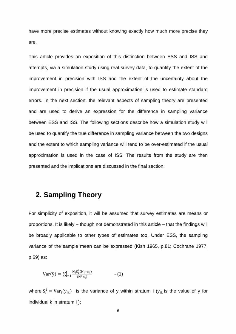
This article provides an exposition of this distinction between ESS and ISS and
attempts, via a simulation study using real survey data, to quantify the extent of the
improvement in precision with ISS and the extent of the uncertainty about the
improvement in precision if the usual approximation is used to estimate standard
errors. In the next section, the relevant aspects of sampling theory are presented
and are used to derive an expression for the difference in sampling variance
between ESS and ISS. The following sections describe how a simulation study will
be used to quantify the true difference in sampling variance between the two designs
and the extent to which sampling variance will tend to be over-estimated if the usual
approximation is used in the case of ISS. The results from the study are then
presented and the implications are discussed in the final section.
2. Sampling Theory
For simplicity of exposition, it will be assumed that survey estimates are means or
proportions. It is likely – though not demonstrated in this article – that the findings will
be broadly applicable to other types of estimates too. Under ESS, the sampling
variance of the sample mean can be expressed (Kish 1965, p.81; Cochrane 1977,
p.69) as:
Var�y�� = ∑ ��� ������
� ������� - (1)
where S�� = Var��y��� is the variance of y within stratum i (y��is the value of y for
individual k in stratum i );
7
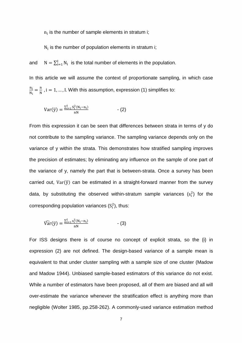
n� is the number of sample elements in stratum i;
N� is the number of population elements in stratum i;
and N = ∑ N����� is the total number of elements in the population.
In this article we will assume the context of proportionate sampling, in which case
��
�= �
, i = 1,… , I. With this assumption, expression (1) simplifies to:
Var�y�� =∑ ��
�!" ������
� - (2)
From this expression it can be seen that differences between strata in terms of y do
not contribute to the sampling variance. The sampling variance depends only on the
variance of y within the strata. This demonstrates how stratified sampling improves
the precision of estimates; by eliminating any influence on the sample of one part of
the variance of y, namely the part that is between-strata. Once a survey has been
carried out, Var�y#� can be estimated in a straight-forward manner from the survey
data, by substituting the observed within-stratum sample variances (s��) for the
corresponding population variances (S��), thus:
Var% �y�� =∑ &�
������ �!"
� - (3)
For ISS designs there is of course no concept of explicit strata, so the {i} in
expression (2) are not defined. The design-based variance of a sample mean is
equivalent to that under cluster sampling with a sample size of one cluster (Madow
and Madow 1944). Unbiased sample-based estimators of this variance do not exist.
While a number of estimators have been proposed, all of them are biased and all will
over-estimate the variance whenever the stratification effect is anything more than
negligible (Wolter 1985, pp.258-262). A commonly-used variance estimation method
8
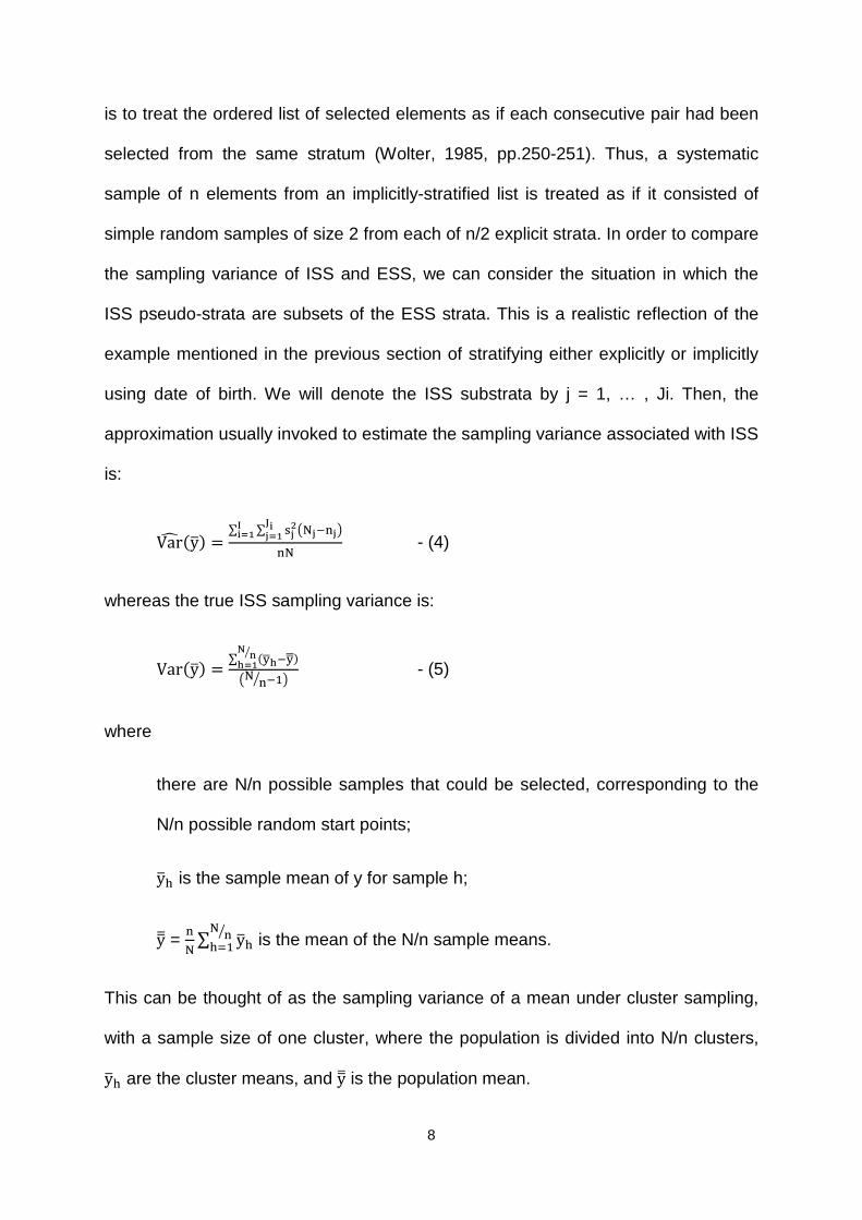
is to treat the ordered list of selected elements as if each consecutive pair had been
selected from the same stratum (Wolter, 1985, pp.250-251). Thus, a systematic
sample of n elements from an implicitly-stratified list is treated as if it consisted of
simple random samples of size 2 from each of n/2 explicit strata. In order to compare
the sampling variance of ISS and ESS, we can consider the situation in which the
ISS pseudo-strata are subsets of the ESS strata. This is a realistic reflection of the
example mentioned in the previous section of stratifying either explicitly or implicitly
using date of birth. We will denote the ISS substrata by j = 1, … , Ji. Then, the
approximation usually invoked to estimate the sampling variance associated with ISS
is:
Var% �y�� =∑ ∑ &'
('��')*�'!"
�!"
� - (4)
whereas the true ISS sampling variance is:
Var�y�� =∑ �+,-�+,,�
. /0-!"
( �0 ��) - (5)
where
there are N/n possible samples that could be selected, corresponding to the
N/n possible random start points;
y�1 is the sample mean of y for sample h;
y�� = �
∑ y�1
�01�� is the mean of the N/n sample means.
This can be thought of as the sampling variance of a mean under cluster sampling,
with a sample size of one cluster, where the population is divided into N/n clusters,
y�1 are the cluster means, and y�� is the population mean.
9
3. Simulation Methodology
Data from wave 1 of Understanding Society, the UK Household Longitudinal Study,
are treated as population data. These data are used to calculate the sampling
variance of means and proportions under simple random sampling, ESS and ISS, in
ways that will be described in this section. Understanding Society is a large
nationally-representative multi-topic general population survey. A stratified, multi-
stage sample of addresses was selected (Lynn, 2009) and all persons aged 16 or
over resident at a sample address were eligible for an individual interview at wave 1.
Members of ethnic minority groups and residents of Northern Ireland were sampled
at higher rates than the remainder of the population. Data collection took place face-
to-face in respondent’s homes using computer-assisted personal interviewing (CAPI)
between January 2009 and March 2011. At wave 1, 50,295 individual interviews
were completed with sample members. For the illustrative purposes of this article,
these individuals are treated as a population from which survey samples are to be
selected.
A set of eleven target parameters were selected for study. Of these, five are means
of continuous variables and six are proportions based on binary variables. For each,
we are interested in comparing the sampling variance of the sample statistic under
alternative sampling designs and the estimate of the ISS sampling variance using
the successive pairing approach. For ease of exposition and calculation, for each
parameter we first amend the population such that N is a multiple of 100. This allows
the subsequent creation of equal-sized explicit strata (each containing 23 = 100
elements) and the application of implicitly stratified systematic sampling designs in
which the sampling interval takes the integer value of 50, the convenience of which
10
will be explained below. From the 50,295 elements, we first drop any with item
missing values. This is done separately for each of the eleven target variables, so
the dropped elements will differ between the eleven simulated populations. Then, a
further set of m elements are dropped (m between 0 and 99) in order to round the
population size down to a multiple of 100. The m elements with the smallest analysis
weights (largest inclusion probabilities) are chosen. Descriptive statistics regarding
this process are presented in Table 1.
For each estimate, the variance and estimated variance for samples of size 2 500 will
be compared under different designs. The following sub-sections describe the
sampling variance metrics that were calculated for each of the eleven parameters to
be estimated. All but one of the metrics rely on knowledge of the population size, N,
and the population variance of y, 6�, each of which were derived in the usual way
from the population simulated as described above.
3.1 Simple Random Sampling
The variance of 7� under simple random sampling is computed as a benchmark and
will be used later in the calculation of design effects for the various sample designs
under consideration, to help with interpretation of the findings. It is calculated in the
usual way:
89:;<;�7�� = ; �=�>�
>= - (6)
11
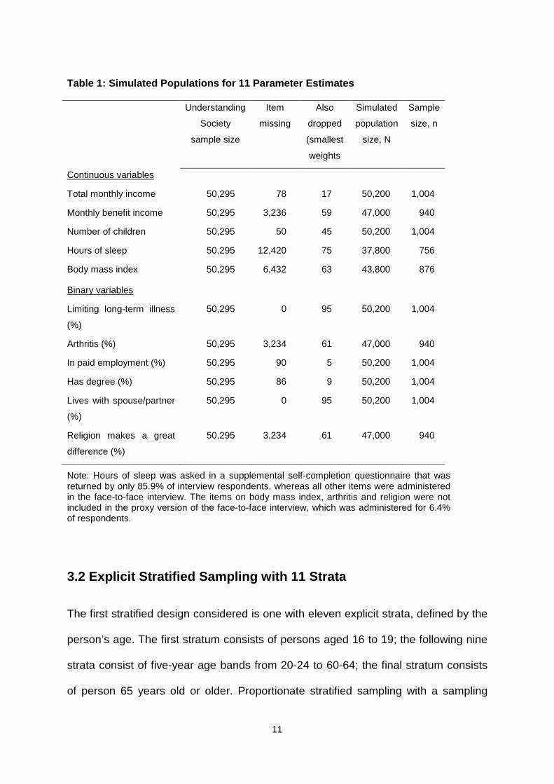
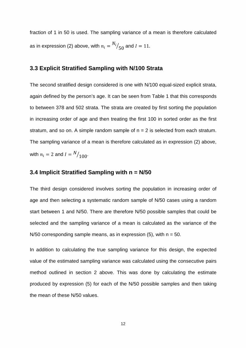
Table 1: Simulated Populations for 11 Parameter Est imates
Understanding
Society
sample size
Item
missing
Also
dropped
(smallest
weights
Simulated
population
size, N
Sample
size, n
Continuous variables
Total monthly income 50,295 78 17 50,200 1,004
Monthly benefit income 50,295 3,236 59 47,000 940
Number of children 50,295 50 45 50,200 1,004
Hours of sleep 50,295 12,420 75 37,800 756
Body mass index 50,295 6,432 63 43,800 876
Binary variables
Limiting long-term illness
(%)
50,295 0 95 50,200 1,004
Arthritis (%) 50,295 3,234 61 47,000 940
In paid employment (%) 50,295 90 5 50,200 1,004
Has degree (%) 50,295 86 9 50,200 1,004
Lives with spouse/partner
(%)
50,295 0 95 50,200 1,004
Religion makes a great
difference (%)
50,295 3,234 61 47,000 940
Note: Hours of sleep was asked in a supplemental self-completion questionnaire that was returned by only 85.9% of interview respondents, whereas all other items were administered in the face-to-face interview. The items on body mass index, arthritis and religion were not included in the proxy version of the face-to-face interview, which was administered for 6.4% of respondents.
3.2 Explicit Stratified Sampling with 11 Strata
The first stratified design considered is one with eleven explicit strata, defined by the
person’s age. The first stratum consists of persons aged 16 to 19; the following nine
strata consist of five-year age bands from 20-24 to 60-64; the final stratum consists
of person 65 years old or older. Proportionate stratified sampling with a sampling
12
fraction of 1 in 50 is used. The sampling variance of a mean is therefore calculated
as in expression (2) above, with ?3 = 23500 and @ = 11.
3.3 Explicit Stratified Sampling with N/100 Strata
The second stratified design considered is one with N/100 equal-sized explicit strata,
again defined by the person’s age. It can be seen from Table 1 that this corresponds
to between 378 and 502 strata. The strata are created by first sorting the population
in increasing order of age and then treating the first 100 in sorted order as the first
stratum, and so on. A simple random sample of n = 2 is selected from each stratum.
The sampling variance of a mean is therefore calculated as in expression (2) above,
with ?3 = 2 and @ = 21000 .
3.4 Implicit Stratified Sampling with n = N/50
The third design considered involves sorting the population in increasing order of
age and then selecting a systematic random sample of N/50 cases using a random
start between 1 and N/50. There are therefore N/50 possible samples that could be
selected and the sampling variance of a mean is calculated as the variance of the
N/50 corresponding sample means, as in expression (5), with n = 50.
In addition to calculating the true sampling variance for this design, the expected
value of the estimated sampling variance was calculated using the consecutive pairs
method outlined in section 2 above. This was done by calculating the estimate
produced by expression (5) for each of the N/50 possible samples and then taking
the mean of these N/50 values.
13
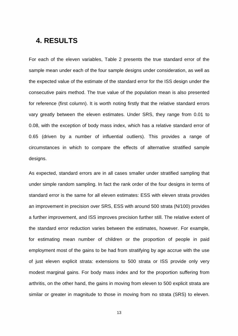
4. RESULTS
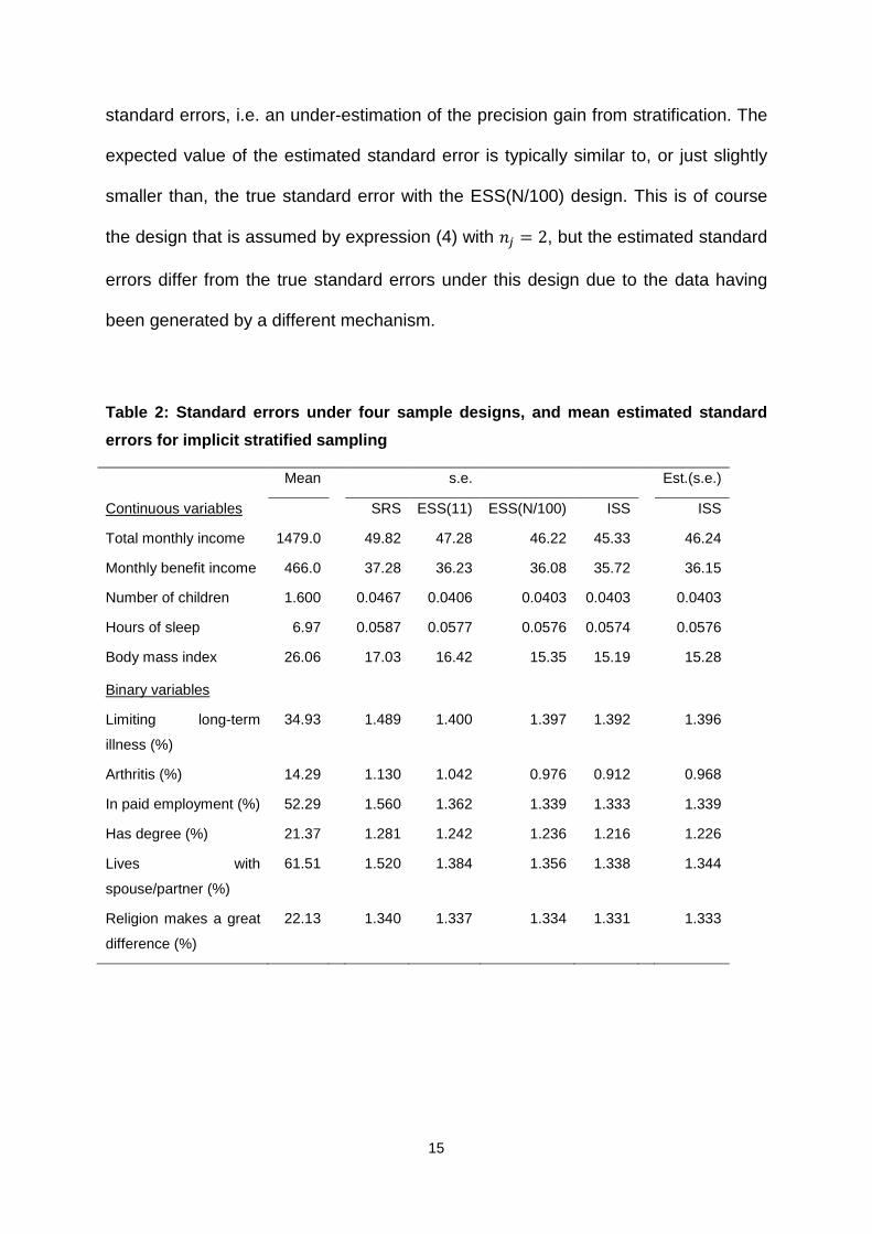
For each of the eleven variables, Table 2 presents the true standard error of the
sample mean under each of the four sample designs under consideration, as well as
the expected value of the estimate of the standard error for the ISS design under the
consecutive pairs method. The true value of the population mean is also presented
for reference (first column). It is worth noting firstly that the relative standard errors
vary greatly between the eleven estimates. Under SRS, they range from 0.01 to
0.08, with the exception of body mass index, which has a relative standard error of
0.65 (driven by a number of influential outliers). This provides a range of
circumstances in which to compare the effects of alternative stratified sample
designs.
As expected, standard errors are in all cases smaller under stratified sampling that
under simple random sampling. In fact the rank order of the four designs in terms of
standard error is the same for all eleven estimates: ESS with eleven strata provides
an improvement in precision over SRS, ESS with around 500 strata (N/100) provides
a further improvement, and ISS improves precision further still. The relative extent of
the standard error reduction varies between the estimates, however. For example,
for estimating mean number of children or the proportion of people in paid
employment most of the gains to be had from stratifying by age accrue with the use
of just eleven explicit strata: extensions to 500 strata or ISS provide only very
modest marginal gains. For body mass index and for the proportion suffering from
arthritis, on the other hand, the gains in moving from eleven to 500 explicit strata are
similar or greater in magnitude to those in moving from no strata (SRS) to eleven.
14
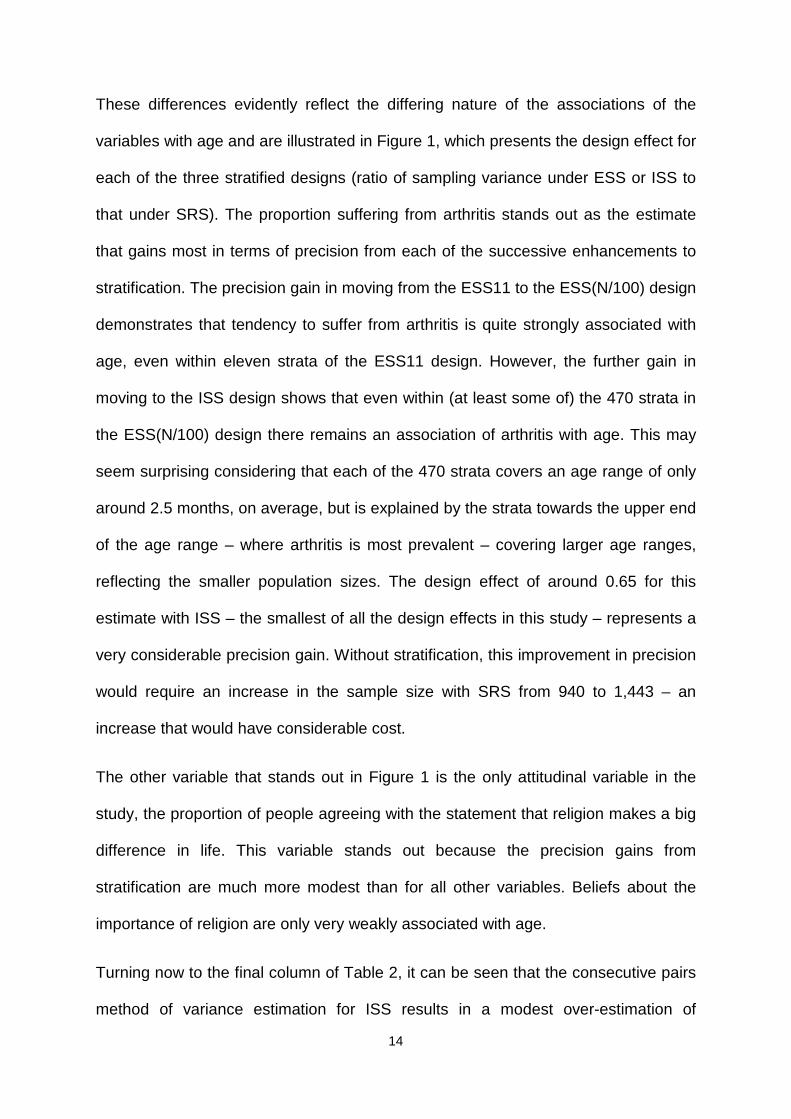
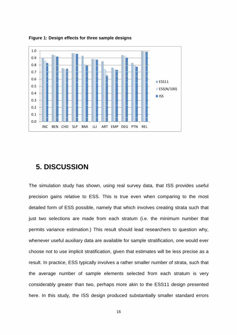
These differences evidently reflect the differing nature of the associations of the
variables with age and are illustrated in Figure 1, which presents the design effect for
each of the three stratified designs (ratio of sampling variance under ESS or ISS to
that under SRS). The proportion suffering from arthritis stands out as the estimate
that gains most in terms of precision from each of the successive enhancements to
stratification. The precision gain in moving from the ESS11 to the ESS(N/100) design
demonstrates that tendency to suffer from arthritis is quite strongly associated with
age, even within eleven strata of the ESS11 design. However, the further gain in
moving to the ISS design shows that even within (at least some of) the 470 strata in
the ESS(N/100) design there remains an association of arthritis with age. This may
seem surprising considering that each of the 470 strata covers an age range of only
around 2.5 months, on average, but is explained by the strata towards the upper end
of the age range – where arthritis is most prevalent – covering larger age ranges,
reflecting the smaller population sizes. The design effect of around 0.65 for this
estimate with ISS – the smallest of all the design effects in this study – represents a
very considerable precision gain. Without stratification, this improvement in precision
would require an increase in the sample size with SRS from 940 to 1,443 – an
increase that would have considerable cost.
The other variable that stands out in Figure 1 is the only attitudinal variable in the
study, the proportion of people agreeing with the statement that religion makes a big
difference in life. This variable stands out because the precision gains from
stratification are much more modest than for all other variables. Beliefs about the
importance of religion are only very weakly associated with age.
Turning now to the final column of Table 2, it can be seen that the consecutive pairs
method of variance estimation for ISS results in a modest over-estimation of
15
standard errors, i.e. an under-estimation of the precision gain from stratification. The
expected value of the estimated standard error is typically similar to, or just slightly
smaller than, the true standard error with the ESS(N/100) design. This is of course
the design that is assumed by expression (4) with ?B = 2, but the estimated standard
errors differ from the true standard errors under this design due to the data having
been generated by a different mechanism.
Table 2: Standard errors under four sample designs, and mean estimated standard
errors for implicit stratified sampling
Mean s.e. Est.(s.e.)
Continuous variables SRS ESS(11) ESS(N/100) ISS ISS
Total monthly income 1479.0 49.82 47.28 46.22 45.33 46.24
Monthly benefit income 466.0 37.28 36.23 36.08 35.72 36.15
Number of children 1.600 0.0467 0.0406 0.0403 0.0403 0.0403
Hours of sleep 6.97 0.0587 0.0577 0.0576 0.0574 0.0576
Body mass index 26.06 17.03 16.42 15.35 15.19 15.28
Binary variables
Limiting long-term
illness (%)
34.93 1.489 1.400 1.397 1.392 1.396
Arthritis (%) 14.29 1.130 1.042 0.976 0.912 0.968
In paid employment (%) 52.29 1.560 1.362 1.339 1.333 1.339
Has degree (%) 21.37 1.281 1.242 1.236 1.216 1.226
Lives with
spouse/partner (%)
61.51 1.520 1.384 1.356 1.338 1.344
Religion makes a great
difference (%)
22.13 1.340 1.337 1.334 1.331 1.333
16
Figure 1: Design effects for three sample designs
5. DISCUSSION
The simulation study has shown, using real survey data, that ISS provides useful
precision gains relative to ESS. This is true even when comparing to the most
detailed form of ESS possible, namely that which involves creating strata such that
just two selections are made from each stratum (i.e. the minimum number that
permits variance estimation.) This result should lead researchers to question why,
whenever useful auxiliary data are available for sample stratification, one would ever
choose not to use implicit stratification, given that estimates will be less precise as a
result. In practice, ESS typically involves a rather smaller number of strata, such that
the average number of sample elements selected from each stratum is very
considerably greater than two, perhaps more akin to the ESS11 design presented
here. In this study, the ISS design produced substantially smaller standard errors
0.0
0.1
0.2
0.3
0.4
0.5
0.6
0.7
0.8
0.9
1.0
INC BEN CHD SLP BMI LLI ART EMP DEG PTN REL
ESS11
ESS(N/100)
ISS
17
than the ESS11 design, so there seems to be a strong case for ISS designs rather
than ESS designs of this kind.
Furthermore, the approximation that must be used to estimate standard errors with
ISS results in only a modest over-estimation. This would make statistical tests
slightly conservative, which is probably more desirable than the false precision that
would be provided by the opposite. In any case, the extent of the over-estimation
(systematic error) is most likely small compared to the extent of sampling variance in
the standard error estimate (random error).
The choice between ESS and ISS would therefore seem to come down to a choice
between improved precision of the survey estimate or unbiased estimation of the
precision of the survey estimate. To take the estimation of the proportion of people
suffering from arthritis as a concrete example, would researchers prefer to have a
standard error of 1.130 associated with their estimate (expected value) of 14.29 and
to have an estimate of the standard error with an expected value of 1.130, or to have
a standard error of 0.912 and an estimate of the standard error with an expected
value of 0.968?
References
Cochrane, W. (1977), Sampling Techniques, 3rd Edition. New York: John Wiley.
Kish, L. (1965), Survey Sampling, New York: John Wiley.
Lynn, P. (2009) “Sample design for Understanding Society.” Understanding Society
Working Paper 2009-01, Colchester: University of Essex.
18
Madow, W. G., and Madow, L. G. (1944), “On the theory of systematic sampling, I”
Annals of Mathematical Statistics, 15, 1–24.
Wolter, K. M. (1985). Introduction to Variance Estimation, Berlin: Springer-Verlag.