The advantages of the general Hartree--Fock method for...

The advantages of the general Hartree-Fock method for future computer simulation of materials

Sharon Hammes-Schiffer and Hans C. Andersen Department of Chemistry, Stanford University, Stanford, California 94305

(Received 6 November 1992; accepted 20 April 1993)

The general Hartree-Fock (GHF) method is a quantum mechanical method for electronic structure calculations that uses a single determinantal wave function with no restrictions on the one-electron orbitals other than orthonormality and the use of a specific basis set. The more familiar restricted Hartree-Fock (RHF) and unrestricted Hartree-Fock (UHF) methods can be regarded as special cases of the GHF method in which additional restrictions are imposed on the occupied orbitals. We propose that the GHF method is very suitable as an electronic structure method to be incorporated into computer simulations that combine the calculation of the Born-Oppenheimer ground state surface with the simulation of the motion of the nuclei on that surface. In particular, for many problems of interest there is only a single GHF minimum of the energy, and the GHF wave function is a continuous function of nuclear positions. The RHF and UHF methods, in comparison, typically have a multiplicity of local minima with curve crossings that generate a discontinuous behavior of the ground electronic state wave function as a function of nuclear positions. In this paper, we use energy minimization techniques to identify and characterize the UHF and GHF electronic minima at fixed nuclear positions for three model systems. The results verify the above assertions and suggest that the GHF method would be more suitable than the RHF or UHF methods for computer simulations.

1. INTRODUCTION

One of the most promising areas of computer simulation of materials is the development of a variety of methods for combining the calculation of the classical dynamics or statistical mechanics of the nuclei on a ground state Born- Oppenheimer (BO) potential surface with the quantum mechanical electronic structure calculation of the BO snr- face itself. This is to be contrasted with the more traditional methods, where the BO potential is represented as a parametrized function of the nuclear positions, typically containing two-body and three-body terms. The newer methods are much more general since they are applicable to systems for which a simple function is inadequate as a representation of the BO surface, such as systems involving covalent bonding.

There are many varieties of the newer computer simulation methods. Each of these methods involves some particular combination of the following: a specific formulation of the quantum electronic structure problem, a specific method of solving this quantum electronic problem, and a specific method for calculating the mechanics or statistical mechanics of the nuclei. We now briefly discuss each of these aspects of computer simulations.

Various formulations of the quantum electronic structure have been used in computer simulations. The two most common formulations are density functional theory,’ both in its spin-compensated and spin-polarized forms, and Hartree-Fock (HF) theory,2 both in its restricted and unrestricted forms. All of these methods introduce a finite discrete basis set so that the solution of the quantum electronic problem involves determining the values of a finite number of coefficients in the wave function.

Several different methods have been used for solving

the quantum electronic problem. The traditional method is to perform a converged numerical variational calculation of the coefficients in the wave function for each nuclear configuration.3 This can be accomplished by solution of the appropriate set of Hartree-Fock-Roothan equations, or more generally by direct attempts to locate the global minimum of an electronic energy functional. Car and Par- rinello formulated an alternative method that converts the electronic structure problem to a classical mechanical problem in which the coefficients are regarded as mechanical variables and the electronic energy functional becomes, in effect, a potential energy for their mechanics4

Finally, the two traditional methods for calculating the classical mechanics or statistical mechanics of the nuclei are molecular dynamics and Metropolis Monte Carlo.

One of the potentially serious problems associated with this class of computer simulation methods is the possibility of multiple solutions of the electronic structure problem. Such multiple solutions may lead to curve crossings at which the BO ground state wave function must “jump” from one solution to the other and hence drastically change its nature. This poses a problem for simulations because the efficient methods of solution of the electronic structure problem all assume, explicitly or implicitly, that the electronic wave function varies smoothly with the nuclear positions. If a global search of the space of wave functions had to be performed at each step to find the ground electronic state or if all of the excited states had to be monitored simultaneously in order to be ready for a curve crossing, then the efficiency of these simulation methods would be seriously compromised, especially for large systems.

This problem can be largely overcome, within the con- text of the Hartree-Fock formulation of the electronic

J. Chem. Phys. 99 (3), 1 August 1993 0021-9606/93/99(3)/1901/13/$6.00 @ 1993 American Institute of Physics 1901

1902 S. Hammes-Schiffer and H. C. Andersen: General Hat-tree-Fock method

structure problem, by the simple but unconventional procedure of using single determinantal wave functions in which there are no restrictions on the occupied molecular orbitals other than orthonormality. This method has been called the general Hartree-Fock (GHF) method, in contrast to the traditional restricted Hartree-Fock (RHF) method and the frequently used unrestricted Hartree-Fock (UHF) method. (Definitions of these terms will be presented in a later section.) We propose that the GHF method is preferable over RI-IF and UHF methods for computer simulations of the type discussed above. Further- more, the analogous generalization of GHF to density functional calculations is likely to have similar advantages over the spin-compensated and spin-polarized forms of density functional theory.

In Sec. II we formulate the GHF method and briefly discuss its history. In Sec. III we present the theory of the GHF method from a perspective that is convenient for the discussion of its use in computer simulations. In particular, we discuss two important properties of a quantum mechanical method that make the method especially useful for the types of computer simulations discussed above. The first property is that there is only one minimum of the energy in the space of wave functions, namely the BO ground state energy. The second property is that the wave function representing -the BO ground state changes continuously as a function of the nuclear coordinates. We assert that the GHF method has these two important properties to a much larger extent than the RI-IF and UHF methods. Sec- tion IV describes the details of the computational methods we have used to implement GHF calculations. Section V discusses many examples to illustrate the properties of the GHF method. Section VI closes with some conclusions.

II. GHF METHOD

A. RHF, UHF, and GHF wave functions

In Hartree-Fock theory, an N-electron system is described by a wave function IY!) represented by a Slater determinant made up of N orthonormal spin orbitals CXi(x>}:

I xtw x2(x1) *** XNW 1

x1(x2) x2w *-* XN(X2) IY~=+? i i : * (1) .

‘XlbN) X2(%) **- XNbN)

The variable x includes both the spatial coordinate r and the spin coordinate w for one electron.

In both restricted Hartree-Fock (RI-IF) and unrestricted Hartree-Fock (UHF) wave functions, each spin orbital is a product of a spatial and a spin part: Xi(x) =k(r)oi(o). The spatial part $(r) is a linear combination of a chosen set of K spatial basis functions {$P(r)):

h(r) = 4 cig$Jr>. (2)

The spin part a(w) of a spin orbital is either a( w ) ra or p(o) ~8, corresponding to spin up or down respectively.

For RHF wave functions, there are equal numbers of a and P spin orbitals, and for each a spin orbital there is also a fi spin orbital with the same spatial part. (In this paper, we use RHF to denote what is sometimes called “closed- shell RHF.“) For open-shell RHF wave functions, some of the spin orbitals are paired as in the closed-shell RHF case, and the remaining spin orbitals are either all a or all fl spin. For UHF wave functions, there are no such restrictions on the spatial parts of the spin orbitals.

In the general Hartre+Fock (GHF) wave function, each spin orbital can contain both a and /3 spin components. A GHF spin orbital can be written as

Xi(X) =$(r>do) +&(r>B(oL (3)

where

q?(r) = il c$$Jr) (4)

and

&b> = p.l 4$#+Ar>. (5)

These equations show that for a system of N electrons and a chosen set of K spatial basis functions, the GHF wave function is specified by 2KN complex coefficients. Thus a GHF wave function for a specific choice of basis set can be represented by a point in the 2KN-dimensional complex space pN, which we will call coefficient space. Since the GHF coefficients must also satisfy the orthonormality constraints, the GHF wave functions lie on a lower dimensionality manifold of the 2KN-dimensional coefficient space. We will refer to this manifold as the GHF manifold, and we will refer to points in this manifold as GHF states.

The spatial basis functions used in a calculation could be chosen to be real, as is typical in molecular calculations using atomic orbital basis functions, or complex, as is the case for calculations using complex plane wave basis functions. When real spatial basis functions are used, it is customary to restrict the coefficients to be real also. In this case, the variational flexibility of the wave function is de- creased, and coefficient space is reduced to a 2KN- dimensional real space. We shall refer to the use of real spatial basis functions and real coefficients as the real general Hartree-Fock (RGHF) method.

A UHF wave function can be regarded as a special case of a GHF wave function, one in which for each orbital i either the {cg} or the {c$> are zero for all p. Hence each UHF wave function corresponds to a point in the same coefficient space that we have just defined, and the set of all UHF wave functions corresponds to a submanifold of the GHF manifold, which we will call the UHF manifold. Sim- ilarly, an RHF wave function can be regarded as a special case of a UHF wave function, one in which there are re- strictive relationships between the cn and 8 coefficients. Hence the set of all RHF wave functions corresponds to a submanifold of the UHF manifold, which we will call the RHF manifold. Finally, when the spatial basis functions

J. Chem. Phys., Vol. 99, No. 3, 1 August 1993

are real, an RGHF wave function is another special case of a GHF wave function, where the imaginary parts of all the coefficients are zero. In this case, the set of all RGHF wave functions corresponds to a submanifold of the GHF manifold, which we will call the RGHF manifold.

The expectation value of the Hamiltonian for a single determinantal GHF wave function of the form of Eq. (1) is a function of the coefficients in the wave function. In other words, it is a function defined for all points in coefficient space:

WIHIW=E(Cc&43). (6)

Here {c$,c$3 denotes the complete set of coefficients needed to specify the spin orbitals in a determinantal wave function. It is important to note that exactly the same function E( Cc& ,43) is applicable to the evaluation of the expectation value of the Hamiltonian for UHF and RHF determinantal wave functions since they also correspond to points in coefficient space. If real basis functions are used, this same energy function is applicable to the RGHF method.

The variational problem for the GHF method is to find the point (or points) in coefficient space that minimizes E( {c~,c$,>) subject to the restriction of being in the GHF manifold or, in other words, subject to the orthonormality constraints. Similarly, the variational problem for the RGHF, UHF, or RHF method is that of finding the point (or points) in coefficient space that minimizes E({cg ,c$)), subject to the restriction of being in the re- spective RGHF, UHF, or RHF manifold. It follows that the global minimum energy for the GHF method will always be lower than or equal to the global minimum for the UHF method, which will always be lower than or equal to the global minimum for the RHF method. Moreover, when the spatial basis functions are real, the global minimum energy for the RGHF method will be less than or equal to that for the UHF method with real coefficients, which will be less than or equal to that for the RHF method with real coefficients.

Before concluding this subsection, we point out that although the GHF wave function is a single determinant, it is actually a type of UHF configuration interaction (CI) wave function. Since each GHF spin orbital is a linear combination of a and p parts, a GHF determinant can be expressed as a linear combination of as many as 2N N-electron UHF determinants. As we will see below, the fact that GHF is a type of UHF-C1 calculation is important for understanding the properties of the method.

B. History of the GHF method and terminology

The history of the GHF method is discussed by Fuku- tome5 and by Lowdin and Mayer.6 The most extensive body of work on this method is that of Fukutome,5 who developed a theory of the symmetry properties of GHF wave functions, the variational stability of solutions of the GHF equations, and the bifurcation of solutions of the equations as the nuclear coordinates change. Moreover, he and his co-workers applied the method to calculate poten-

tial energy curves for a variety of systems. More recently Lowdin and Mayer applied the method to atoms and molecules.6 For a useful perspective on Fukutome’s work and its relationship to other problems involving electronic cor- relation, see a review by Calais.7

The terminology to denote the various types of methods is not entirely standardized. We shall follow Calais7 and Lowdin and Mayer6 and use the phrase “general HartreeFock (GHF)” to denote methods that use a single determinantal wave function with no restrictions on the orbitals (other than orthonormality of the occupied orbitals and perhaps the use of a specific basis set). The orbitals can be mixtures of a and p spin, the coefficients in the orbitals can be complex, and there are no necessary relationships among the coefficients other than orthonormality of the occupied orbitals. This method is denoted “unrestricted Hartree-Fock (UHF)” by Fukutome,5 but such a designation conflicts with the more customary usage of UHF to denote a determinant in which each orbital has purely a or p character.

III. GHF THEORY

A. Symmetry operators

As noted above, Fukutome has given an extensive and elegant discussion of the symmetry properties of GHF wave functions.5 His analysis and classification of states is especially appropriate for molecular electronic structure calculations. In computer simulations, however, the electronic state is represented by the coefficients of the spin orbitals instead of the determinant itself. Thus it is worth- while to focus on the symmetry properties in coefficient space rather than in wave function space.

The first type of operator of concern is an arbitrary unitary transformation of the spin orbitals in a determinant. Since a unitary transformation preserves the orthonormality of the spin orbitals, it maps states in the GHF manifold into the GHF manifold. Moreover, a unitary transformation of a set of spin orbitals gives a new set of spin orbitals whose determinantal wave function differs from the original one by at most just a phase factor of unit magnitude. Hence any expectation value is invariant to such a unitary transformation.

The second type of operator of concern is a spin rotation. A spin rotation operator is a linear operator that affects the spin part of a spin orbital’in the following way:

Ma(a) =cos(8/2>exp( --i#/2)a+sin(6/2)exp(i+/2)8,

Mfi(fi) = -sin(8/2)exp( -i#42)a+cos(O/2>exp(@/2)/3, (7)

where fi is a unit vector and 13 and $ are its spherical polar angles. Since Mfi is linear, it has the following effect on a spin orbital of the form of Eq. (3):

WJlj3rkdw) +$%Mw)l =$~(r>Mfi(a> +#(rMdB). (8) If, for a specific fi, we apply Mfi to all of the spin

orbitals of a determinant, the result is another determinant.

S. Hammes-Schiffer and H. C. Andersen: General Hat-tree-Fock method 1903



This procedure will be referred to as a spin rotation. A spin rotation is equivalent to a rotation of the axes of the coordinate system used to define the components of spin without a corresponding rotation of the axes used to define positions in space. Since it preserves the orthonormality of the spin orbitals, it maps the GHF manifold onto itself. If the Hamiltonian contains no terms dependent on the electron spin, it is easy to show that the expectation value of the Hamiltonian is unchanged by such an operation. More- over, it is easy to show that the magnitude of the expectation value of the total spin vector S is also unchanged by such a mapping, although its direction is of course changed. Note that the quantity referred to here, which we will call the total spin magnitude, is

B. Symmetry operations for RHF, UHF, and RGHF determinants

The more restricted HF methods have a smaller group of symmetry operations, which we summarize here.

For the RGI-IF method, the group of symmetry operations includes the set of real orthogonal (as opposed to unitary) transformations of the orbitals, the set of spin rotation mappings with #=O or +=2?r, and products of these operators. (Time reversal is a special case of a spin rotation for real orbitals and real coe5cients with 0 =0 and 8=7-r.)

I @>I =(~~,~2+~~y~2+~~z~2)1’2, (9)

which is distinctly different from the expectation values of spin that are normally of concern in electronic structure theory.

For the UHF method, the group of symmetry operators includes the subset of unitary transformations of the orbitals that mix the a orbitals among themselves and that mix the /3 orbitals among themselves, the set of spin rotations with 8=0 or 0=~, time reversal, and all products of these operators.

The third type of operator is time reversal. When act- ing on a spin orbital of the form of Eq. (3), it has the following effect:

For the RHF method and the open-shell RHF method, the group of symmetry operators includes the set of unitary transformations that mixes the paired a orbitals together in the same way that the paired p orbitals are mixed, the set of spin rotations with 8=0 or 8=n, time reversal, and all products of these operators.

(10) The time reversal operator T for a determinant is the si- multaneous application of t to each spin orbital in the determinant. Since time reversal also preserves the orthonormality of the spin orbitals, it maps the GHF manifold onto itself. In addition, it is easy to show that the expectation value of the Hamiltonian and the total spin magnitude are unchanged by such a mapping.

C. Relationship between our classification of methods and Fukutome’s symmetry classification of HF wave functions

The set of all operators of these three types are, in effect, symmetry operations on coefficient space that map the GHF manifold onto itself and that leave important properties of the determinantal wave function unchanged, including the expectation value of the Hamiltonian (provided it is spin independent) and the total spin magnitude. Moreover, an arbitrary sequence of such operators has the same features, and the set of all such sequences is a group of symmetry operations. Two GHF states will be called equivalent if one can be obtained from the other by application of some member of this group of symmetry operations.

Fukutome’s extensive classification of the possible symmetries of HF wave functions is an especially useful one.5 The review of Calais is helpful in interpreting the classification.7 For the convenience of the reader, we now summarize the relationship between the various methods discussed in this paper and the corresponding symmetry classes of Fukutome.

The method that we denote GHF is the most general HF method and can have solutions of all of Fukutome’s symmetry types.

From the definition of equivalence it is clear that a GHF state can be equivalent to a UHF or RHF state without itself being in the UHF or RHF manifold. We point out that for RHF and UHF wave functions, the expectation value of the total spin vector must be in the positive or negative 2 direction, and the total spin magnitude must be a half-integer. In contrast, it is easy to show that for GHF wave functions, the expectation value of the total spin vector can point in an arbitrary direction, and the total spin magnitude is not necessarily half-integer. Note that since the total spin magnitude is the same for two equivalent states, if a GHF state is equivalent to a UHF state then its total spin magnitude must be a half-integer.

The method that we denote RGHF (with real spatial functions and real coefficients) generates solutions that fall into the symmetry classes denoted torsional spin density wave (TSDW), axial spin density wave (ASDW), and time reversal invariant closed shell (TICS). To our knowl- edge, for problems of chemical interest these are the only symmetry types of interest for generating the ground state BO potential curves. Thus, we suspect that in practice the RGHF method has all the variational flexibility of the GHF method.

The methods that we denote UHF and open-shell RHF generate solutions that fall into the S axial and S invariant classes [namely axial spin current wave (ASCW), ASDW, axial spin wave (ASW), TICS, and charge current wave (CCW)]. The customary methods for implementing UHF and open-shell RHF use real spatial functions and real coefficients. The solutions then fall into a subset of the classes just mentioned, namely ASDW and TICS.

The method that we denote RHF generates solutions that fall into the S invariant classes, namely TICS and


CCW. If real basis functions and real coefficients are used, then the solutions fall into just the TICS class.

D. Definition of a single global minimum and of continuity of the wave function

As discussed above, all equivalent states (related by symmetry operations) have exactly the same energy for a spin-independent Hamiltonian. Therefore, when we refer to the “global minimum” in the GHF manifold, we are actually referring to at least a set of equivalent states. More generally, the global minimum might correspond to a set of states with the same energy, not all of which are equivalent to one another. (This latter situation is certainly not the usual one. Any such degeneracy between states that are not equivalent would represent an accidental degeneracy or perhaps one that is generated by some spatial symmetry in the problem.) In order to facilitate precise discussions about the number of distinct global minima (or local minima or saddle points), we now present a definition of a single global minimum (or local minimum or saddle point).

If a point in the GHF manifold has the global minimum energy, then it and all other points with this energy that form a connected region in the GHF manifold shall be regarded as part of the same global minimum. Moreover, all other points that are equivalent to this connected set shall be regarded as part of the same minimum. Thus a global minimum consists of a connected set of points plus zero or more other connected sets that are equivalent to the first set. Using the same idea we can define a local minimum and a saddle point, each of which is a set of points. (The same can be done for UHF and RHF methods, tak- ing into account that, for these methods, the appropriate manifold of coefficient space is of lower dimensionality and fewer symmetry operations are available to generate equivalent states.) With such a definition of a minimum, the number of distinct local minima or global minima becomes a well-defined concept.

With this in mind, we next define the continuity of a wave function as a function of nuclear positions when the wave function is represented in a simulation by a point in coe5cient space. At each nuclear configuration, there is a set of points in coefficient space at which the energy is equal to its global minimum value. This set consists of one or more global minima in the sense defined above. In a simulation, the particular point in this set that is deter- mined to be the solution of the electronic problem is most likely dependent on the algorithm used and on the previous history of the simulation. (In a simulation of the Car- Parrinello type, the point in coe5cient space will vibrate in the vicinity of the set of minimum energy points, occasion- ally being in the set.) As the nuclei move, the location of this set of points in coefficient space changes.

Given this situation, we will define two types of continuity of the wave function: a strong form and a weak form. In strong continuity, every point in one set becomes infln- itesimally close to some point in the second set as the nuclear configuration of the second set approaches that of the tist set. In weak continuity, at least one point in the

first set becomes infinitesimally close to some point in the second set as the nuclear configuration of the second set approaches that of the first set. We now discuss why at least one of these types of continuity is necessary to make algorithms for solving the electronic problem function properly as the nuclei are moved.

E. Continuity of the wave function as a function of nuclear positions

When performing computer simulations by any of the methods discussed in the first section of the paper, the electronic problem must be solved again and again (in some way or other) as the nuclei are moved. Typically the solution for one set of nuclear positions is the starting point for the solution at the next set of nuclear positions. Hence it is important that the ground state electronic wave function, or its representation as a point in coefficient space (for HF methods), be a continuous function of the nuclear position. Otherwise, the solution of the electronic problem would become at each step a global search for a minimum electronic energy rather than a local search.

There are some situations in which the exact wave function is a discontinuous function of nuclear positions. For example, if the usual electrostatic Hamiltonian (without spin-dependent terms) is used, this can happen if the two lowest energy states have different spin multiplicity and cross at a particular nuclear configuration. The exact ground state wave function then jumps discontinuously from one spin multiplicity to another as the nuclei are moved through this nuclear configuration. (When spin- orbit interactions are included in the Hamiltonian, such discontinuous jumps are eliminated, and adiabatic potential energy curves that do not cross are generated.) In such situations, the discontinuity is caused by the intrinsic physics of the system being simulated. As we will see below, the GHF method can eliminate this type of discontinuity in an unusual way.

There are other situations in which the exact ground state wave function is a continuous function of nuclear positions, but an approximate ground state wave function is a discontinuous function of nuclear positions. In this case, the discontinuity is an artifact of the approximate method used to obtain the ground electronic state. The most common way for this to happen in HF methods is if the two lowest energy single determinantal states have the same spin multiplicity and cross at a particular nuclear configuration. The single determinantal ground state wave function then jumps discontinuously from one such state to another as the nuclei are moved through this nuclear configuration. Such crossings are artifacts of the HF method and are not a feature of the exact wave functions. If the more accurate configuration interaction (CI) method is used, where the wave function is represented by a linear combination of two or more determinants, then adiabatic potential curves that avoid this crossing are generated, and the wave function is a continuous function of the nuclear positions in the avoided crossing region. Thus the continuity property of the exact wave function is recovered only when a method more accurate than the RHF or UHF

S. Hammes-Schiffer and H. C. Andersen: General Hat-tree-Fock method 1905


1906

I Y

S. Hammes-Schiffer and H. C. Andersen: General Hat-tree-Fock method

method is used. As we shall see below, the CI character of the GHF single determinantal wave function allows it to eliminate these kinds of discontinuities.

Curve crossings and the resulting discontinuities in the wave function can cause severe problems in simulations. For example, if the electrons are in their true ground state for an initial set of nuclear positions, then as the nuclei move they may stay on the diabatic curve and end up in an excited electronic state. In addition, this diabatic curve may eventually “end” if the wave function ceases to be a local minimum or a stationary point. What actually hap- pens in the simulation at this point depends on the algorithm used, but the result is an unphysical event.

The RHF and UHF methods are very susceptible to this type of difficulty. The main point of this paper is that with the GHF and RGHF methods these problems are much less likely to occur and perhaps will never occur in problems for which HF methods are accurate. To see why this is true, we now discuss the relationships between the global minimum and other stationary points for the various HF methods.

F. Local and global minima in the UHF and GHF manifolds

From here on, we shall restrict our attention to GHF and UHF wave functions. As noted above, the variational problem for the GHF (or UHF) method is equivalent to finding the global minimum of the energy in the GHF (or UHF) manifold of coefficient space. These manifolds might, in general, have additional stationary points in the form of local minima, maxima, and saddle points.

Here we consider the relationships among the local and global minima and stationary points in the form of a set of assertions, which are either empirical observations, theorems, or conjectures.

1. In typical problems involving small numbers of atoms, for some range of nuclear positions each state in the GHF global minimum is equivalent to a UHF state, which in such a case is also necessarily in the global minimum in the UHF manifold. In other words, under certain circumstances the extra flexibility inherent in the GHF wave function relative to the UHF wave function, for a given basis set, leads to no lower a value of the energy. However, for other ranges of the nuclear positions, the GHF global minimum energy is lower than the UHF global minimum energy. There are many examples of this in Sec. V.

2. In typical problems, there are several local minima in the UHF manifold. The potential energy curves as a function of nuclear position, generated by these many minima, frequently cross one another. The UHF BO ground state potential energy curve then has cusps at such crossing points, and the UHF global minimum wave function is a discontinuous function of nuclear position at these points. We will give numerical examples of this in Sec. V.

3. The states in a stationary point (either a global min-

imum, a local minimum or maximum, or a saddle point) in the UHF manifold are also necessarily in a stationary point in the GHF manifold. The proof of this is elementary and will be omitted.

4. In many cases, a point that is in a local minimum in the UHF manifold is in merely a saddle point, i.e., not a local minimum, in the GHF manifold. Again, examples of this will be presented in Sec. V.

5. In contrast to observation 2 above, we strongly suspect that the following is true. For problems in which the GHF method is accurate, there is a single local minimum in the GHF manifold, namely the GHF global minimum; when there is more than one local minimum, the GHF method is not accurate. We shall refer to this as the strong form of the “single minimum hypothesis,” in contrast with the weak form, which is as follows. For problems in which the GHF method is accurate, there is only one global minimum in the GHF manifold (in the sense defined above).

These statements contain the notion of the “accuracy” of the GHF method. The notion of accuracy that we are using can be defined using the approach of Fukutome.5 For any particular system (i.e., a set of nuclear positions and a certain number of electrons) and any particular basis set, the RHF eigenfunctions of S2 and S, (which are, in general, linear combinations of RHF single determinants) form a complete set of functions that span the finite- dimensional vector space of N-electron wave functions that are linear combinations of determinants constructed using the basis. Thus any GHF determinant can be expressed as a linear combination of such RHF configurations. More- over, the exact ground state wave function (subject to the same limitations on basis set) can also be expressed the same way. A semiquantitative measure of the accuracy of the GHF method (i.e., of the extent to which the exact ground state can be represented as a single GHF determinant) is obtained by observing whether the GHF wave function contains, with significant weight, all of the RHF configurations that contribute to the exact ground state.

If the strong form of the single minimum hypothesis holds, i.e., there exists only a single minimum, then the GHF method will be very convenient for computer simulations for two reasons. First, the solution of the electronic problem involves linding the global minimum, which is clearly facilitated by having no local minima in which a direct minimization algorithm could be trapped. Second, the existence of only a single local minimum makes it much less likely that curve crossings could generate a wave function that changes discontinuously with nuclear positions.

Most of the advantages of the strong form, however, can actually be realized if the weak form is valid. If the weak form of the hypothesis holds, then the search for a global minimum will not be trapped by excited local minima provided the search is started close enough to the global minimum (such as with values of the coefficients that represent the global minimum of the previous nuclear configuration in a simulation). Moreover, similar to the


strong form, discontinuities in the ground state wave function as a function of nuclear position would be much less likely to occur.

We have no general proof of either the strong or the weak form of this hypothesis, but we do have empirical evidence of their validity. Much of the rest of the paper is devoted to a discussion of examples, some from our own calculations and some from previously published work by others, that lend support to the strong and weak forms of the hypothesis. We will show many instances in which there is only a single GHF minimum. The only situations that we have found in which there is more than one local minimum are those in which the GHF method is not accurate, in the sense discussed above. (In these situations, of course, the RHF and UHF wave functions will also be inaccurate, since they are variationally less flexible than the GHF wave functions. )

IV. COMPUTATIONAL DETAILS

The calculations presented in this paper involve energy minimizations to determine the electronic ground states of simple systems. In all cases we used real spatial basis functions, and we restricted the coefficients in the occupied spin orbitals to be real. Thus the RGHF, rather than the GHF, method is being tested. Whenever we performed UHF calculations, we also used real spatial basis functions and restricted the coefficients in the occupied spin orbitals to be real, as is commonly done in calculations that are denoted “UHF.” The calculations required the evaluation of quantum mechanical matrix elements, a method for minimizing the electronic energy with respect to the orbital coefficients, and methods for testing whether a state is a local minimum or a saddle point.

For the calculations on carbon and nitrogen atoms, we used a Huzinaga-Dunning full double-zeta basis set. For the systems we studied containing hydrogen and lithium atoms, we used an STO-3G basis set. In the case of the lithium atoms, we used a frozen-core approximation* so that we could consider the 1s core electrons as part of the nucleus and apply the variational principle to only the valence molecular orbitals.

Our electronic energy minimization algorithm is based on the Car-Parrinello molecular dynamics method.4 We will just give a brief summary of the method. The reader is referred to the review articles of Madden and Payne and co-workers9 for more details on the .general method and to the article by Chacham and Mohallem” for similar appli- cations of the Car-Parrinello method to electronic energy minimization.

For a given nuclear configuration, the electronic energy is specified by a set of coefficients describing the spatial part of the spin orbitals that make up the determinantal wave function, as discussed in Sec. II. Since the spin orbitals must be orthonormal, there are constraints imposed on the coefficients. The energy minimization consists of searching coefficient space for the set of coefficients satisfying the orthonormalization constraints and giving the lowest energy.

The coefficients can be viewed as the coordinates of fictitious particles of mass m, where m is just a fictitious mass. Then we introduce a fictitious time t that represents the movement through coefficient space, and we can calculate coefficient velocities, which are defined as the first derivatives of the coefficients with respect to t. Thus for a system of N electrons and K basis functions, there is a fictitious kinetic energy

T=fmi 5 (I~~[2i-I$p12) (11) i fi

and the potential energy is equal to the HF electronic energy: V=E{c&,c$}. The Lagrangian for this system is T- V, subject to the orthonormality constraints

Uij({C~,C$})= x (C~C~~+~~~~)S,,-sij=O, (12) PV

where Spy is the overlap integral between basis functions $fi and 4,.

This Lagrangian gives rise to the following equations of motion:

aa- rnCk= -‘$+ C /2ij 2, (13)

rp i P where the ilij are Lagrange multipliers and k indicates the spin ((I: or /3). In order to do the constrained dynamics, we used the RATTLE algorithm,” which is based on the veloc- ity form of the Verlet algorithm.

In this paper we are only interested in energy minimizations and not in dynamics simulations, so we modified the RATTLE algorithm. In particular, whenever the energy increased during a time step, we returned to the previous coefficients, zeroed all of the velocities, and restarted the dynamics. This procedure was repeated until the energy no longer changed by more than a given tolerance. For systems where convergence of a GHF wave function was difficult, the stopping condition was modified to require that neither the energy nor the total spin magnitude was chang- ing by more than the given tolerances. This helps ensure that the actual minimum is obtained because the total spin magnitude is often more sensitive than the energy to small changes in the coefficients.

In many of the examples given in Sec. V, we wanted to verify the existence of only a single minimum. Thus we developed methods of searching for local minima, checking the stability of stationary points, and determining whether two states are equivalent. We now briefly describe these methods.

In order to search for local minima, we applied the energy minimization procedure described above with numerous different starting coefficients. The starting coefficients were obtained by generating a random set of coefficients with magnitude less than or equal to one and then symmetrically orthonormalizing these coefficients. We call this method the random search technique.

We used two different methods to test the stability of states. The first method involves perturbing the coefficients of the state by a small amount and applying the energy minimization procedure starting with these perturbed coefficients and zero velocities. If the new state has a lower

S. Hammes-Schiffer and H. C. Andersen: General Hartree-Fock method 1907



energy than the original state, then the original state was not stable (unless the perturbation was too large). How- ever, if the new state has the same energy as the original state for numerous different random perturbations, then this is strong evidence that the original state is stable. This method is not exact because it clearly depends on the magnitude and direction of the perturbation. Nevertheless, if a variety of perturbations are applied, then the method is quite reliable. We call this method the perturbative stability test.

The second stability test is exact but only applies to the stability of UHF states in the GHF manifold. This method relies on the theorem that a particular UHF local minimum described by the determinant 1 Y,) is unstable in the GHF manifold if we are able to find another UHF determinant 1 YB) that satisfies the following two conditions. First, it must be the same as jY,J except for one orbital, whose spatial part can be different from and whose spin must be opposite to that of the original orbital. Second, the energy E, of 1 YB) must be less than the energy EA of 1 YA). If we can find such a determinant ) Y J, the proof of the instability of the UHF local minimum (‘u,) in the GHF manifold is as follows.

A general property of determinants is that the linear combination of two determinants that differ only by one row or one column is also a determinant. Thus, we can form a GHF determinant I Yc) from a linear combination of the two normalized UHF determinants I YA) and I Y & : IY,)=c,l‘u, )+c,lY&. Since I‘u,) and IYB) areeigen- functions of S, with different eigenvalues, we know that ( YA ( Y B) =O. , Therefore, introducing the new variable 8 and normalizing ( Y & gives C~=COS 0 and cB=sin 8. The energy EC of I Yc) is then simply E,=EA cos2 8 +EB sin2 8. Since this function decreases monotonically for 0<8<9~/2, we have proven that I Y,) (i.e., 0=0) is not a local minimum in the GHF manifold because there is a direction to fall directly from this state to a lower energy state, namely IYB) (i.e., e=d2).

In order to apply this stability test to a determinant representing a UHF local minimum, we flip each of the UHF orbitals one at a time and randomly perturb the spatial part of this flipped orbital, maintaining orthonormality by Gram-Schmidt orthonormalization of the flipped orbital. If one of these perturbed determinants has a lower energy than the original determinant, then we have found a determinant satisfying the criteria discussed above and have thus proven that this particular UHF local minimum is unstable in the GHF manifold. We call this method the exact stability test.

In addition to testing the stability of states, we often want to determine whether two states are equivalent. In order to absolutely verify the equivalence of two states, the symmetry operations connecting the two states must be obtained. Since this is a difficult procedure, we instead assume that two states are equivalent if their energy and total spin magnitude are the same within our numerical uncer- tainty.

Finally, we point out that since all UHF local minima are stationary points in the GHF manifold, any algorithm

that is unable to break the UHF symmetry could mistake a UHF local minimum for a GHF local minimum. This becomes a problem during GHF calculations when for some nuclear configurations the GHF minimum is equivalent to a UHF state, but for other nuclear configurations this UHF state becomes a GHF saddle point. This situation occurred in the GHF simulations presented in Sec. V C, where the electronic energy was fully converged for each nuclear configuration. If the coefficients of the previous nuclear configuration were used as a starting point for the calculation at each new nuclear configuration, then the algorithm was unable to break any existing UHF symmetry and could mistake a GHF saddle point (corresponding to a UHF local minimum) for a GHF local minimum. Thus, in order to break the UHF symmetry during GHF calculations, we randomly perturbed the coefficients by an average of 10% before the energy minimization at each new nuclear configuration.

V. RESULTS AND DISCUSSION

In this section we present various results to show that in many situations there is only one local minimum, namely the global minimum, in the GHF manifold. More- over, in those situations for which more than one local minimum is found, it can be shown that the GHF method is not accurate. This will confirm the strong and weak forms of the single minimum hypothesis. We also present results that illustrate the behavior of the RGHF potential energy curves as contrasted with those generated by the UHF method. A. Atoms

For one-electron systems and the usual electrostatic Hamiltonian, a straightforward extension of the usual der- ivation of the variational principle shows that there is just one distinct local minimum for the GHF method with a specific basis set. (The same is also true of the UHF and open-shell RHF methods for a one-electron system.) The first nontrivial test of the single minimum hypothesis then occurs for many-electron atoms. We have performed calculations on six- and seven-electron atoms, namely carbon and nitrogen. The following procedure was applied to each of the two atoms using a double-zeta basis set.

We used the random search technique 20 times to find RGHF local minima. The same local minimum was found in each case, which we assume is the global minimum. We also used the random search technique 20 times for each spin multiplicity to find UHF local minima. We found only one local minimum for each spin multiplicity, and the lowest of these was equivalent to the RGHF global minimum. We then applied the perturbative stability test to the excited UHF local minima in the GHF manifold and found all of them to be unstable. Thus for these two atoms, both forms of the single minimum hypothesis were confirmed.

For atoms with larger atomic numbers and smaller spacings between the orbital energies, it is possible that the


GHF single determinantal method will not be an accurate representation of the ground state and that there will be several distinct minima in the GHF manifold.

8. Molecular systems

1. Previously published results

The extensive work of Fukutome and co-workers,5 as well as that of Ltiwdin and Mayer,6 provide many case studies of the GHF method applied to small molecular systems. Fukutome’s work was especially concerned with the question of the stability of the RHF and UHF solutions, i.e., whether a solution represents a local minimum or a saddle point in the GHF manifold. It was also concerned with bifurcations of the solutions at the onset of instabilities. At such a bifurcation, a solution that is stable for some range of nuclear coordinates branches into one stable solution and one unstable solution of higher energy as the nuclear positions change. By using the theory of bifurcations developed by Fukutome, we were able to draw conclusions about the stability or instability of excited state potential energy curves from the data given in Fukutome’s examples, even when the information was not explicitly given.

Fukutome used semiempirical and ab initio matrix elements to study the GHF method and the potential energy curves and electronic states it generates for a variety of systems.5 These systems included the dissociation curves of HZ, Nz, 02, and CO; the internal rotation of C,H,; bond angle bending in the carbenes CH,, CHF, and CF,, and in OS; the dimerization of the carbenes; and the H3 and H4 systems in various symmetric configurations. Lijwdin and Mayer investigated the dissociation curves of the Hz and BH molecules6 A careful reading of these papers and close examination of the figures reveals that in all these cases, and for all nuclear positions investigated, the global minimum in the GHF manifold is the only local minimum found in the GHF manifold, with just one exception, that of co.

The CO BO potential energy diagram (see Fig. 47 in Ref. 5) has three states that represent local minima for a range of distances whose lower limit is about 1.43 A. For some internuclear distances, the three local minimum GHF states consist of one state with RHF character and two states with UHF character (denoted ASW and ASDW, in Ref. 5). For others, there are three local minimum GHF states of UHF character (denoted ASDW,, ASW, and ASDW,) as well as a saddle point of RHF character. Fukutome’ performed an extensive analysis of the exact ground state for CO with his basis set and con- cluded that for this range of distances CO is a system for which a single determinant, even of the GHF type, is not an accurate representation of the ground state, in the sense discussed above.

Thus, all the data presented in the work of Fukutome and co-workers’ and Liiwdin and Mayer6 are consistent with the strong and weak forms of the single minimum hypothesis. Moreover, these papers contain many examples that illustrate the assertions made above in Sec. III F,

0 I I z :::I \>bcr/y+ :: 0.02 1 c

30 40 50 60 70 80 angle (degrees)

0.60 (b)


0.00 4 V

30 40 50 60 70 80 angle (degrees)

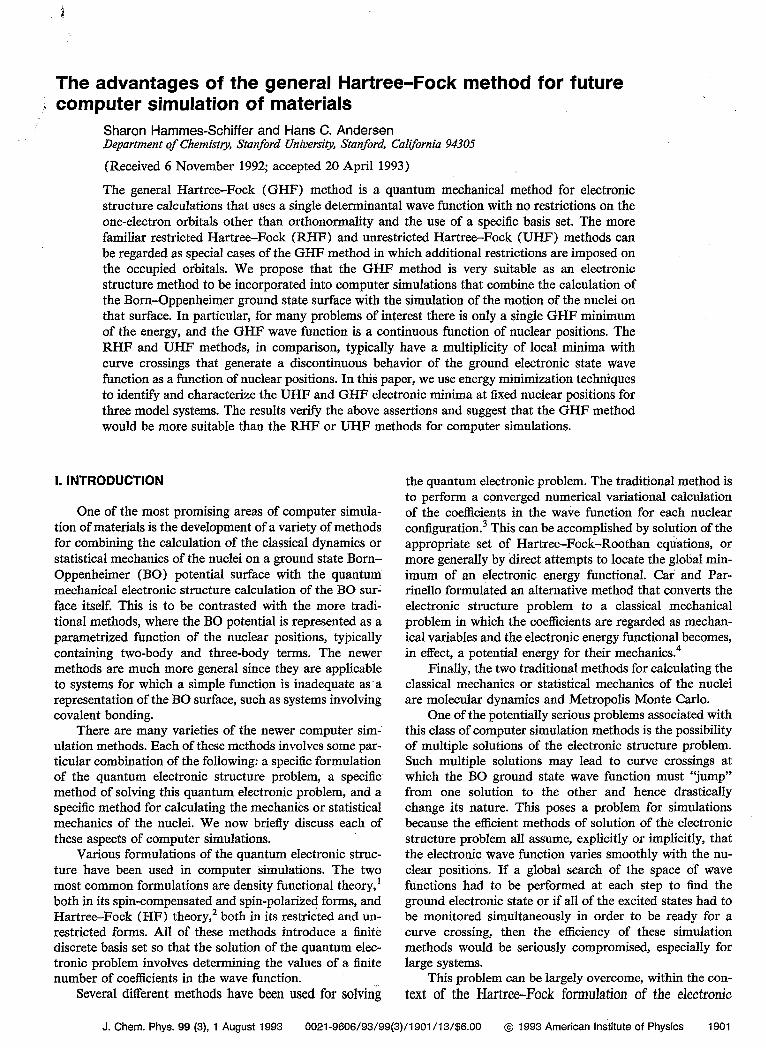
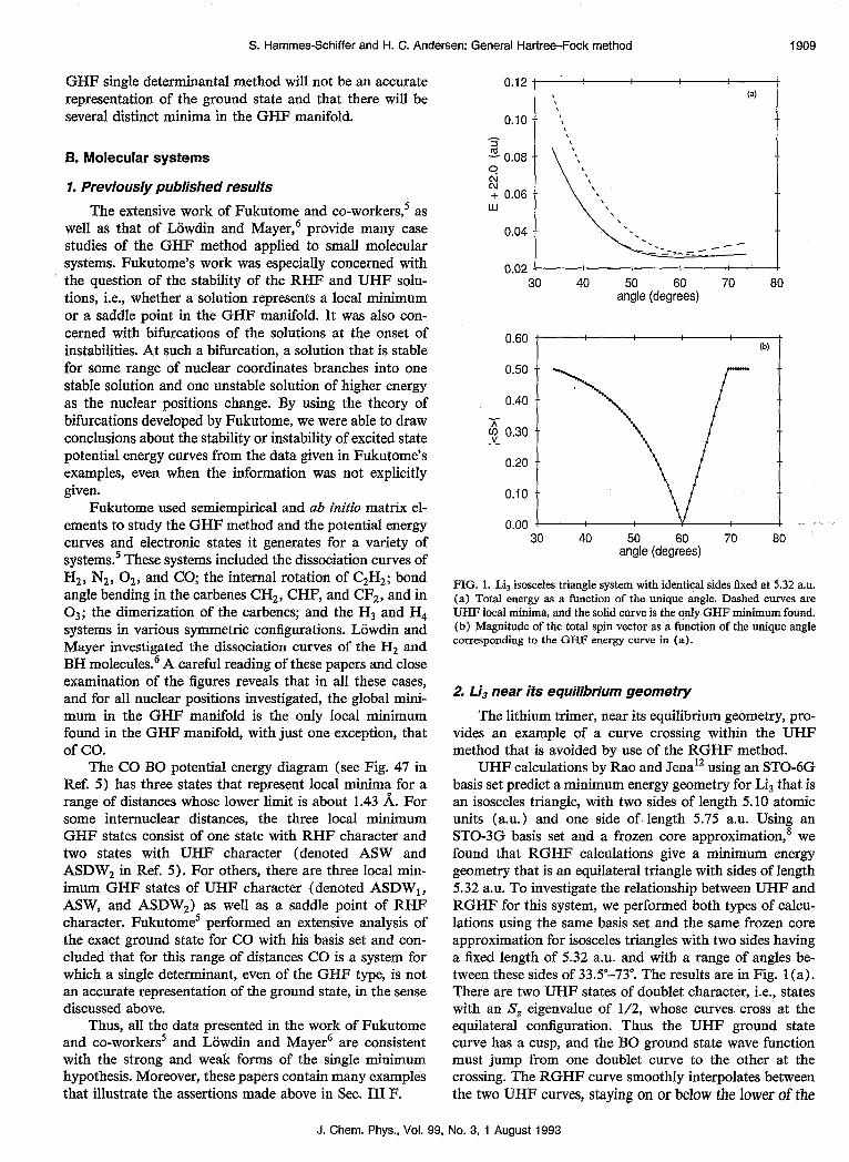
FIG. 1. Lij isosceles triangle system with identical sides fixed at 5.32 a.u. (a) Total energy as a function of the unique angle. Dashed curves are UHF local minima, and the solid curve is the qnly GHF minimum found. (b) Magnitude of the total spin vector as a function of the unique angle corresponding to the GIW energy curve in (a).

2. Li3 near its equilibrium geometry

The lithium trimer, near its equilibrium geometry, pro- vides an example of a curve crossing within the UHF method that is avoided by use of the RGHF method.

UHF calculations by Rao and Jena12 using an STOdG basis set predict a minimum energy geometry for Lis that is an isosceles triangle, with two sides of length 5.10 atomic units (a.u.> and one side of length 5.75 a.u. Using an STO-3G basis set and a frozen core approximation,* we found that RGHF calculations give a minimum energy geometry that is an equilateral triangle with sides of length 5.32 a.u. To investigate the relationship between UHF and RGHF for this system, we performed both types of calculations using the same basis set and the same frozen core approximation for isosceles triangles with two sides having a fixed length of 5.32 a.u. and with a range of angles between these sides of 33.5”-73”. The results are in Fig. 1 (a). There are two UHF states of doublet character, i.e., states with an S, eigenvalue of l/2, whose curves. cross at the equilateral configuration. Thus the UHF ground state curve has a cusp, and the BO ground state wave function must jump from one doublet curve to the other at the crossing. The RGHF curve smoothly interpolates between the two UHF curves, staying on or below the lower of the


1910

d ” il

S. Hammes-Schiffer and H. C. Andersen: General Hat-tree-Fock method

two. The total spin magnitude of the RGHF wave function is shown in Fig. 1 (b) . It has a value of 0.5 when the RGHF minimum is equivalent to one of the doublet UHF minima, but near the UHF curve crossing it decreases so that at an angle of 60” the RGHF total spin magnitude is zero. This illustrates the ability of the RGHF method to generate adiabatic potential energy curves without cusps, unlike the diabatic curves generated by the UHF method. This is possible for the RGHF method because of the CI character of a GHF wave function.

We applied the perturbative stability test to 30 points on each UHF curve in the region where the RGHF global minimum was lower than the lower UHF curve. We con- sistently found that the UHF states are saddle points in the RGHF manifold whenever they are not equivalent to the RGHF global minimum. We also searched for RGHF local minima by using the random search technique ten times for each geometry spaced 1” apart for the range of angles shown in the figures. We never found any RGHF local minima other than the global minimum. Thus, all the results are consistent with the strong and weak forms of the single minimum hypothesis for this system.

Note that the GHF wave function predicts an equilateral triangle as the equilibrium geometry, whereas RHF, UHF, and CI wave functions predict isosceles triangles as the equilibrium geometry.‘2*‘3 Thus the GHF wave function can predict slightly incorrect equilibrium geometries if it smooths over a curve crossing by creating a minimum rather than a maximum. This is simply a mathematical artifact of the GHF wave function, however, and will not affect the dynamics significantly because the difference between the minimum UHF energy and the minimum GHF energy is only on the order of 10B3 a.u., and the UHF equilibrium geometry is close to an equilateral triangle. The dynamics would be much more adversely affected if the higher energy UHF electronic state were misinter- preted as the global minimum.

To conclude this subsection on molecular systems, we point out that we have also applied the GHF method to larger lithium clusters, both neutral and cationic, of up to five atoms.’ All of our results from these studies are consistent with the strong and weak.forms of the single minimum hypothesis.

C. Interaction of several open shell atoms

Fukutome presented calculations for a system of four hydrogen atoms in a set of symmetric configurations.5 As noted above, his results indicate that for each set of nuclear configurations studied, there is only one local minimum in the GHF manifold, namely the GHF global minimum.

Here we present some results for systems of three and four hydrogen atoms in less symmetric configurations to illustrate the ,behavior of the UHF and RGHF methods in the situations more commonly encountered in computer simulations of materials. In particular, any simulation of a gas of open-shell atoms should exhibit the features dis- played below, and most likely these features will also exist for condensed phases.

0 D

(-l&5.8)

0 C ---------------------+

(-6.0,2.4)

0 s 0 A

(-2.0,O.O) (2.0.0.0)

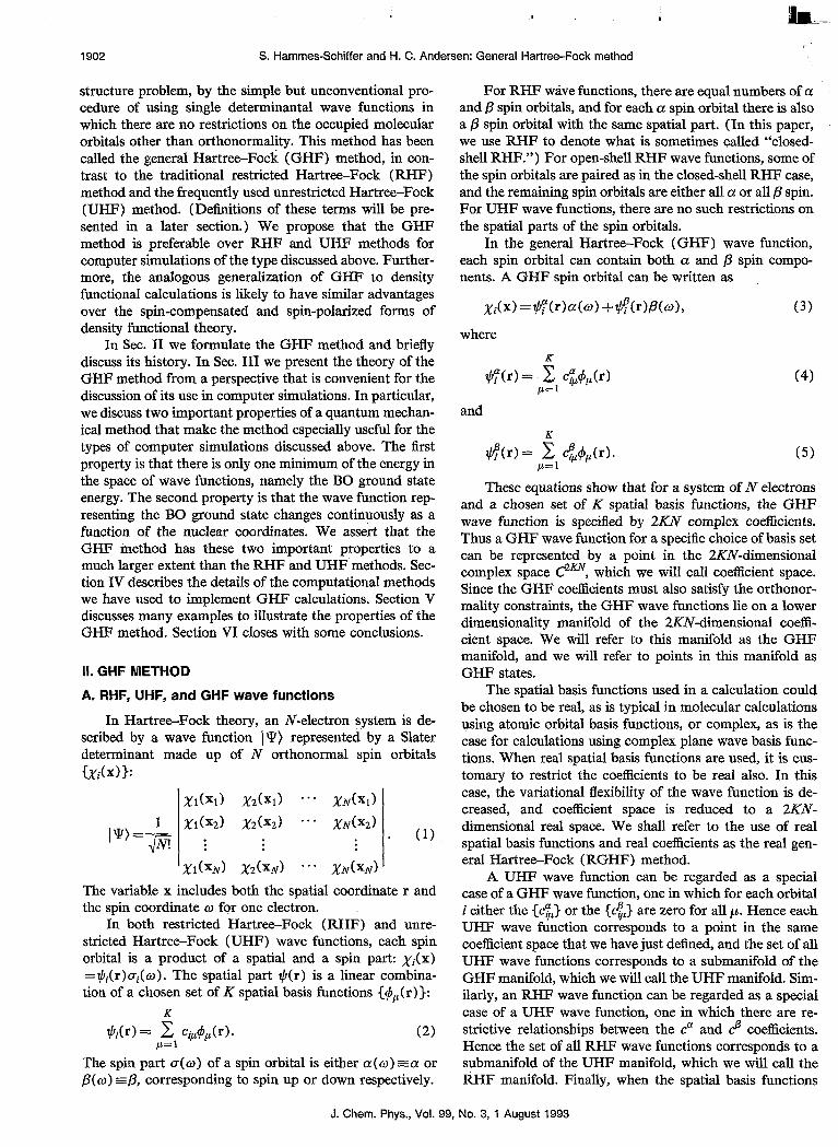
FIG. 2. Placement of hydrogen atoms HR , HB , and H, in H3 system and hydrogen atoms HA, H,, Hc, and H, in H4 system. All atoms are stationary except for atom H,, which moves from xy coordinates (-6.0,2.4) to (6.0,2.4), as indicated by the dashed arrow.

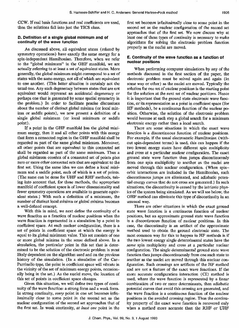
The first such example we present is a system containing three hydrogen atoms in the xy plane, as shown in Fig. 2. The first atom HA is fixed at (2.0,0.0), and the second atom HB is fixed at coordinates ( -2.0,O.O). We investigate the BO curves as a third atom Hc travels along a line parallel to the x axis with yc=2.4. This third atom H, starts at xc= -6.0 and ends up at x,=6.0. We chose the distances between the hydrogen atoms to be large enough to prevent strong chemical bonds. Under these conditions each of the three UHF molecular orbitals is centered mainly on one of the three atoms. Thus, for UHF wave functions, each atom has an electron that has mainly either pure a or pure fi spin. There are four UHF energy curves, as shown in Fig. 3 (a). The three lower curves correspond to doublet states with an S, eigenvalue of l/2, and the fourth curve corresponds to a quartet state with an S, eigenvalue of 3/2.

We calculated the RGHF energy curves by starting with random coefficients to compute the energy at the first geometry and then moving the third atom Ho with regular steps, using the previous solution as a starting point for the , next step and breaking the symmetry of each starting point as discussed in Sec. IV. The result is shown in Fig. 3(a). Starting at xc= - 6.0, the RGHF curve first coincides with UHF curve 3, then crosses to the UHF curve 1, and finally crosses to the UHF curve 2. A closer look at the crossing between UHF curves 1 and 3 at xc= - 1.2 is shown in Fig. 3 (b) . This figure shows the RGHF curve smoothly crossing from one UHF curve to the other. We also examined the total spin magnitude, which is shown in Fig. 3(c). We can see that the RGHF minimum has the total spin magnitude of a doublet UHF state, 0.5, on either side of the crossing, but the RGHF total spin magnitude decreases to about 0.49 at the curve crossing. Thus, Figs. 3 (b) and 3 (c) show that the RGHF global minimum is equivalent to the UHF global minimum except for the region close to the crossing.

The smoothness of the RGHF energy curve at the UHF curve crossing clearly shows the ability of an RGHF wave function to eliminate cusps due to curve crossings of the same spin multiplicity. As discussed in Sec. II, this smooth interpolation arises from the CI character of the



-1.46 7 -6 -4 -2 0 2 4 6

xc b-0

7.0 2 PI

.’ y 6.5-e ,’ __

I

4.5 * t -3 -2 -1 0 1 2 3

0.505

0.500

$ 0.495

0.490

0.465

L (

c -3

103(x, + 1.2) (au)

-2 -1 0 1 2 103(xc+ 1.2) (au)

+ 3

FIG. 3. Ha system as described in the text. (a) Energy as a function of the x coordinate of atom Hc (xc). Dashed curves are UHF local minima. Using the following notation to distinguish the curves: curve-spin (HA), spin (HJ, spin (Hc), the UHF curves are I--t t L; 2-l t?; 3--tit; 4-f T t. The solid curve is the only GHF minimum found. (b) Magnifi- cation of (a) near the curve crossing between UHF curves 1 and 3 at ~~~-1.2. (c) Magnitude of the total spin vector as a function of xc corresponding to the GHF energy curve in (b).

RGHF wave function and reflects the physically correct behavior of the exact wave function given the usual electrostatic Hamiltonian. Moreover, these results illustrate the straightforward way in which the RGHF method, unlike the UHF method, generates a BO ground state curve with a wave function that is a continuous function of nuclear position and an energy that avoids getting trapped in excited local minima.

The reason for this behavior is simply that there ap- pears to be only one local minimum in the RGHF manifold for this system, in accordance with the single minimum hypothesis. To verify this, we performed the following tests. We applied the exact stability test to the UHF local minima in the RGHF manifold for 40 configurations regularly spaced along each of the four UHF curves. All UHF minima that were higher in energy than the RGHF minimum were found to be unstable. In order to search for other RGHF local minima, we used the random search method ten times for each of the 40 configurations. We always obtained the same energy as that obtained in the construction of the RGHF curve by the method described above.

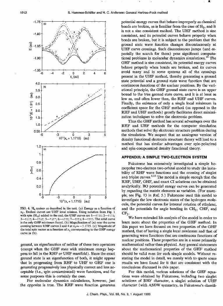
The second example we are presenting is the same as the first one except that a fourth atom HD is placed at coordinates (- 1.5,5.8), as shown in Fig. 2. This has the effect of splitting each of the UHF curves from the previous example so that we have a total of eight UHF curves, as shown in Fig. 4(a). The upper curve is a quintet with an S, eigenvalue of 2, where all of the spins are aligned, and the lower seven curves are singlets and triplets.

The RGHF energy and total spin magnitude curves were calculated in the same way as described above. The main difference in the results is that now the avoided curve crossings are between curves of different spin multiplicities, namely a singlet and a triplet. From Fig. 4 (a) we can see that, starting at xc= - 6.0, the RGHF curve first coincides with the singlet UHF curve 2, then crosses to the triplet UHF curve 4, and finally crosses to the singlet UHF curve 3. Figures 4(b) and 4(c) show the energy and total spin magnitude at the crossing between the UHF curves 2 and 4 at xc= - 1.1715. Note that the RGHF energy curve is smooth in the region of this crossing. Figure 4(c) shows that the RGHF total spin magnitude is 0 when the RGHF minimum is equivalent to the singlet UHF minimum and increases smoothly until it is equal to 1 when the RGHF minimum is equivalent to the triplet UHF minimum.

These results illustrate the way in which the RGHF method generates a cuspless BO ground state curve, with a continuous wave function, that stays on or below the lowest UHF curve and avoids the crossings even of UHF curves of dijg”erent multiplicity. In contrast to the first example, this smooth interpolation is not physically correct given the usual electrostatic Hamiltonian but is rather a mathematical artifact of the GHF wave function. Never- theless, it is advantageous for simulations that intend to study the behavior on the ground state BO curve. As in the previous example, we performed a similar number of exact stability tests of the UHF states in the RGHF manifold and random searches for additional local minima in the RGHF manifold. We found that for each nuclear configuration, the strong and weak forms of the single minimum hypothesis hold for this system as well.

VI. CONCLUSIONS

Whereas an RHF wave function is an eigenstate of S2 and S,, and a UHF wave function is an eigenfunction of the latter but not the former, a GHF wave function is, in


1912

d Y il

S. Hammes-Schiffer and H. C. Andersen: General Hartree-Fock method

-1.95 4 -6 -4 -2 0 2 4 6

‘xc (au)

4.0 (b)

3.5 /’

‘; 2.5 .- s ; 2.0 -- w fl 1.5.-

1.0 .. /

0.50 1 ’ -5 -3 0 3 5

103(xc+ 1.1715) (au)

1.2 (4

1 .-

0.8 --

3 0.6--

0.4 --

0.2 ..

0- -5 -3 0 3 5

103(xc+ 1.1715) (au)

FIG. 4. H, system as described in the text. (a) Energy as a function of xc. Dashed curves are UHF local minima. Using notation from Fig. 1 with spin (II,) added to the end, the UHF curves are l--t t IL; 2-l 1 t I; 3--t&St; 4--Tt&t; 5--tltt; dlttt; 7--tttl; I--tttt. Thesolid curve is the only GHF minimum found. (b) Magnification of (a) near the curve crossing between UHF curves 2 and 4 at xc= - 1.17 15. (c) Magnitude of the total spin vector as a function of xc corresponding to the GHF energy curve in (b).

general, an eigenfunction of neither of these two operators (except when the GHF state with minimum energy hap- pens to fall in the RHF or UHF manifold). Since the exact ground state is an eigenfunction of both, it might appear that in progressing from RHF to UHF to GHF one is generating progressively less physically correct and less ac- ceptable (i.e., spin contaminated) wave functions, and for some purposes this is certainly the case.

For molecular dynamics calculations, however, just the opposite is true. The RHF wave function generates

potential energy curves that behave improperly as chemical bonds are broken, as is familiar from the case of H,, and it is not a size consistent method. The UHF method is size consistent, and its potential curves behave properly when bonds are broken, but it is subject to the problem that the ground state wave function changes discontinuously at UHF curve crossings. Such discontinuous jumps (and especially the search for them) pose significant computational problems in molecular dynamics simulations.‘4 The GHF method is size consistent, its potential energy curves behave properly when bonds are broken, and its curves avoid many and in some systems all of the crossings present in the UHF method, thereby generating a ground state potential and a ground state wave function that are continuous functions of the nuclear positions. By the variational principle, the GHF ground state curve is an upper bound to the true ground state curve, and it is at least as low as, and often lower than, the RHF and UHF curves. Finally, the existence of only a single local minimum in coefficient space for the GHF method (as opposed to the RHF and UHF methods) greatly facilitates direct minimization techniques to solve the electronic problem.

Thus the GHF method has several advantages over the RHF and UHF methods for the computer simulation methods that solve the electronic structure problem during the simulation. We suspect that an analogous version of density functional electronic structure theory will lead to a method that has similar advantages over spin-polarized and spin-compensated density functional theory.

APPENDIX: A SIMPLE TWO-ELECTRON SYSTEM

Fukutome has extensively investigated a simple ho- mopolar two-electron two-orbital model to study the instability of RHF wave functions and the crossing of singlet and triplet curves.5715 The model is simple enough that the RHF, UHF, GHF, and exact CI solutions can be obtained analytically. BO potential energy curves can be generated by regarding the matrix elements as variables. (For example, see Fig. 13 in Ref. 5.) Fukutome used this model to investigate the low electronic states of the hydrogen mole- cule, the potential curves for internal rotation of ethylene, and the potentials for angle bending in CH,, CHF, and CF,.

We have extended his analysis of the model in order to learn more about the properties of the GHF method. In this paper we have focused on two properties of the GHF method, that of having a single local minimum and that of generating wave functions that are continuous functions of nuclear positions. These properties are in a sense primarily mathematical rather than physical. Any general statements about the mathematical properties of the GHF method should be valid even for such simple models. Without re- stating the model in detail, we merely wish to quote some results we have found for it that are consistent with the conclusions discussed in this paper.

For this model, various solutions of the GHF equations were obtained by Fukutome, including two singlet solutions of RHF character, a singlet solution of UHF character (with ASDW symmetry, in Fukutome’s classifi-



cation), and a triplet solution of open-shell RHF character. A crossing of the singlet UHF and triplet curves was found. (See Fig. 13 in Ref. 5.) Fukutome performed an extensive stability analysis of the various states. From his results, it is clear that except at the singlet-triplet crossing, there is only one local minimum in GHF space, namely the global minimum, which confirms the validity of both forms of the single minimum hypothesis for this system. At the crossing points, however, two distinctly different and de- generate solutions exist, apparently in violation of the single minimum hypothesis. We have analyzed this situation and found that at the crossing point there is also a series of solutions of GHF character and TSDW symmetry. These solutions form a connected continuum of solutions that include the singlet ASDW solution and the triplet solution as limiting cases. Thus, in coefficient space, there is actually a single connected GHF global minimum even at this crossing point, again validating both forms of the single minimum hypothesis.

Furthermore, we can choose the values of the matrix elements of this two-electron system so that the following is true: the only minima are the RHF singlet solutions; the UHF singlet solution (ASDW) no longer exists; and the triplet RHF solution is unstable and always higher in energy than the RHF singlet global minimum. (Using the notation in Ref. 5, this will happen when r < - 1.) The two RHF singlet solutions cross and for some nuclear configurations are both local minima. (Using the notation in Ref. 5, the region where there is more than one local minimum is for 1 +r < q < - 1 -r. ) This does not violate the single minimum hypothesis, however, because for these nuclear configurations the single determinantal GHF wave function is not an accurate representation of the ground state. This is due to the fact that for these nuclear configurations the exact ground state has large contributions from both singlet RHF states, whereas the single determinantal GHF minimum is either one or the other singlet RHF state. Thus this example also validates both forms of the single minimum hypothesis.

ACKNOWLEDGMENTS

We thank Dr. C. Janssen for the use of his ab initio Gaussian integral program and E. D. Remy for advice on

its implementation. We also thank Dr. W. Kob for many helpful discussions. This work was supported by the Na- tional Science Foundation Grant No. CHE-89 18841 and benefited from computer resources provided by the Na- tional Science Foundation through Grant No. CHE- 8821737. S.H.-S. was supported by a National Science Foundation graduate fellowship and a grant from the AT&T Bell Laboratories Graduate Research Program for Women.

‘See, for example, F. Ancilotto, W. Andreoni, A. Selloni, R. Car, and M. Parrinello, Phys. Rev. Lett. 65, 3148 (1990); R. N. Bamett, U. Land- man, A. Nitzan, and G. Rajagopal, J. Chem. Phys. 94, 608 (1991); F. Buda, G. L. Chiarotti, R. Car, and M. Parrinello, Phys. Rev. Lett. 63, 294 (1989); E. S. Fois, A. Selloni, M. Parrinello, and R. Car, J. Phys. Chem. 92, 3268 (1988); D. Hohl, R. 0. Jones, R. Car, and M. Par- rinello, J. Chem. Phys. 89, 6823 (1988); R. Kawai and J. H. Weare, Phys. Rev. Lett. 65, 80 (1990); U. Rijthlisberger and W. Andreoni, J. Chem. Phys. 94,8129 (1991); A. St-Amant and D. R. Salahub, Chem. Phys. Lett. 169, 387 (1990).

‘See, for example, M. J. Field, J. Phys. Chem. 95, 5104 (1991); M. J. Field, J. Chem. Phys. 96, 4583 (1992); B. Hartke and E. A. Carter, Chem. Phys. Lett. 189, 358 (1992).

3See, for example, M. J. Field, P. A. Bash, and M. Karplus, J. Comput. Chem. 11, 700 (1990); U. C. Singh and P. A. Kollman, ibid. 7, 718 (1986); I. S. Wang and M. Karplus, J. Am. Chem. Sot. 95, 8160 (1973); A. Warshel and M. Karplus, ibid. 94, 5612 (1972).

4R. Car and M. Parrinello, Phys. Rev. Lett. 55, 2471 (1985). ‘H. Fukutome, Int. J. Quantum Chem. 20, 955 (1981), and references

therein. ‘P.-O. Liiwdin and I. Mayer, Adv. Quantum Chem. 24, 79 (1992). 7J.-L. Calais, Adv. Quantum Chem. 17, 225 (1985). as. Hammes-SchitTer and H. C. Andersen, J. Chem. Phys. 99, 523

(1993). ‘D. K. Remler and P. A. Madden, Mol. Phys. 70, 921 (1990); M. C.

Payne, M. P. Teter, and D. C. Allan, J. Chem. Sot. Faraday Trans. 86, 1221 (1990).

‘OH. Chacham and J. R. Mohallem, Mol. Phys. 70, 391 (1990). “H. C. Andersen, J. Comput. Phys. 52, 24 (1983). “B. K. Rao and P. Jena, Phys. Rev. B 32, 2058 (1985). 131. Boustani, W. Pewestorf, P. Fantucci, V. Bonacic-Koutecky, and J.

Koutecky, Phys. Rev. B 35, 9437 (1987); D. W. Davies and G. Del Conde, Chem. Phys. 12, 45 (1976).

i4The generalized valence bond perfect pairing method, used recently for ab initio dynamics by B. Hartke and E. A. Carter [J. Chem. Phys. 97, 6569 (1992)], has similar problems as the UHF method because there are situations in which the pairing scheme must change discontinuously as the nuclei are moved.

“H. Fukutome, Prog. Theor. Phys. 47, 1156 (1972); 50, 1433 (1973).


Date post:	12-Mar-2018
Category:	Documents
Upload:	lenhi
View:	286 times
Download:	4 times

The advantages of the general Hartree--Fock method for...

Documents