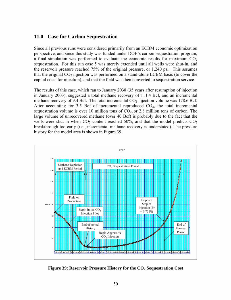
The Allison Unit CO2 – ECBM Pilot: A Reservoir Modeling Study

1

The Allison Unit CO2 – ECBM Pilot: A Reservoir Modeling Study Topical Report January 1, 2000 – June 30, 2002 Scott Reeves, Anne Taillefert and Larry Pekot Advanced Resources International 9801 Westheimer, Suite 805 Houston, TX 77042 and Chris Clarkson Burlington Resources Suite 3700 250-6 Ave. S.W. Canada, T2P 3H7 U.S. Department of Energy Award Number DE-FC26-0NT40924 February, 2003

i

Disclaimers

U.S. Department of Energy This report was prepared as an account of work sponsored by an agency of the United States Government. Neither the United Sates Government nor any agency thereof, nor any of their employees, makes any warranty, express or implied, or assumes any legal liability or responsibility for the accuracy, completeness, or usefulness of any information, apparatus, product, or process disclosed, or represents that its use would not infringe privately owned rights. Reference herein to any specific commercial product, process, or service by trade name, trademark, manufacturer, or otherwise does not necessarily constitute or imply its endorsement, recommendation, or favoring by the United States Government or any agency thereof. The views and opinions of authors expressed herein do not necessarily state or reflect those of the United Sates Government or any agency thereof.

Advanced Resources International The material in this Report is intended for general information only. Any use of this material in relation to any specific application should be based on independent examination and verification of its unrestricted applicability for such use and on a determination of suitability for the application by professionally qualified personnel. No license under any Advanced Resources International, Inc., patents or other proprietary interest is implied by the publication of this Report. Those making use of or relying upon the material assume all risks and liability arising from such use or reliance.

ii

Abstract

In October, 2000, the United States Department of Energy, through contractor Advanced Resources International (ARI), launched a multi-year government-industry research & development collaboration called the Coal-Seq project. The Coal-Seq project is investigating the feasibility of carbon dioxide (CO2) sequestration in deep, unmineable coalseams by performing detailed reservoir studies of two enhanced coalbed methane (ECBM) recovery field projects in the San Juan basin. The two sites are the Allison Unit, operated by Burlington Resources, and into which CO2 is being injected, and the Tiffany Unit, operating by BP America, into which nitrogen (N2) is being injected (the interest in understanding the N2-ECBM process has important implications for CO2 sequestration via flue-gas injection). The purposes of the field studies are to understand the reservoir mechanisms of CO2 and N2 injection into coalseams, demonstrate the practical effectiveness of the ECBM and sequestration processes, demonstrate an engineering capability to model them, and to evaluate sequestration economics. In support of these efforts, laboratory and theoretical studies are also being performed to understand and model multi-component isotherm behavior, and coal permeability changes due to swelling with CO2 injection. This report describes the results of an important component of the overall project, the Allison Unit reservoir study. The Allison Unit is located in the northern New Mexico portion of the prolific San Juan basin. The study area consists of 16 methane production wells, 4 CO2 injection wells, and one pressure observation well. The field originally began production in July 1989, and CO2 injection operations for ECBM purposes commenced in April, 1995. CO2 injection was suspended in August, 2001, to evaluate the results of the pilot. In this study, a detailed reservoir characterization of the field was developed, the field history was matched using the COMET2 reservoir simulator, and future field performance was forecast under various operating conditions. Based on the results of the study, the following conclusions have been drawn:

o The injection of CO2 at the Allison Unit has resulted in incremental methane recovery over estimated ultimate primary recovery, in a proportion of approximately one volume of methane for every three volumes of CO2 injected.

o The study area was successfully modeled with ARI’s COMET2 model. However, aspects of the model remain uncertain, such as producing and injecting bottomhole pressures, CO2 content profiles of the produced gas, and the pressure at the observation well.

o There appears to be clear evidence of significant coal permeability reduction with CO2 injection. This permeability reduction, and the associated impact on CO2 injectivity, compromised incremental methane recoveries and project economics. Finding ways to overcome and/or prevent this effect is therefore an important topic for future research.

o From a CO2 sequestration standpoint, the incremental methane recoveries (based solely on the conditions encountered at the Allison Unit), can provide a meaningful offset to CO2 separation, capture and transportation costs, on the order of $2–5/ton of CO2.

iii

Table of Contents

Page 1.0 Introduction............................................................................................................. 1

2.0 CO2-ECBM Process................................................................................................ 2

3.0 Site Description....................................................................................................... 4

4.0 Reservoir Description ............................................................................................. 9

5.0 Model Construction .............................................................................................. 19

6.0 Initial Model Results............................................................................................. 23

7.0 History Matching .................................................................................................. 27

7.1 Permeability ................................................................................................. 27 7.2 Sorption Behavior ........................................................................................ 30

8.0 Performance Forecasts .......................................................................................... 35

9.0 Discussion of Results............................................................................................ 44

10.0 Economic Assessment .......................................................................................... 47

11.0 Case for Carbon Sequestration.............................................................................. 50

12.0 Conclusions........................................................................................................... 52

13.0 Nomenclature........................................................................................................ 53

14.0 Acknowledgements............................................................................................... 55

15.0 References............................................................................................................. 56

Appendix A: Comparison Plots - Initialization Run versus Actual Data ...................... A-1

iv

List of Tables

Page Table 1: Allison Unit Basic Coal Reservoir Data............................................................... 8

Table 2: Langmuir Constants, by Layer ........................................................................... 12

Table 3: Layer Sorption Properties and Distribution of Methane Resource..................... 12

Table 4: Estimated Permeability Function Parameters..................................................... 17

Table 5: Reservoir Parameters used in Simulation Model................................................ 21

Table 6: Estimated Skin Factor Changes Due to Recavitation ......................................... 22

Table 7: Case 2 – Incremental Methane Recoveries by Well .......................................... 38

Table 8: Summary of Model Forecast Results................................................................. 43

Table 9: Economic Analysis Assumptions ...................................................................... 47

Table 10: Economic Analysis Results: Case 2 versus Case 1 ........................................ 47

Table 11: Economic Analysis Results, Cases 3, 4, 5, 6 versus Case 2 ............................ 48

v

List of Figures

Page Figure 1: Sorption Isotherms for CO2, CH4 and N2 on Wet San Juan Basin Coal ............. 2

Figure 2: Location of the Allison Unit, San Juan Basin ..................................................... 4

Figure 3: Producer/Injector Well Pattern, Allison Unit ...................................................... 5

Figure 4: Producing History, Allison Unit Study Area....................................................... 7

Figure 5: Producing History, Individual Allison Unit Well ............................................... 7

Figure 6: Structure Map, Yellow Coal (units in feet above sea level)................................ 9

Figure 7: Total Net Coal Isopach, Allison Unit Study Area (units in feet) ........................ 9

Figure 8: Langmuir Volume vs. Coal Density Correlation, Methane............................... 10

Figure 9: Langmuir Volume vs. Coal Density Correlation, Carbon Dioxide................... 10

Figure 10: Methane Sorption Isotherms, Allison Unit Study Area .................................. 11

Figure 11: Carbon Dioxide Sorption Isotherms, Allison Unit Study Area....................... 11

Figure 12: Relative Permeability Curves, Allison Unit .................................................... 13

Figure 13: Porosity Map, Allison Unit (units in fractions)............................................... 14

Figure 14: Comparison of Relative Permeability Curves ................................................. 14

Figure 15: Correlation between Effective Gas and Absolute Permeability...................... 15

Figure 16: Permeability Map for Allison Unit.................................................................. 16

Figure 17: Permeability Changes with Pressure and Concentration................................. 18

Figure 18: Map View of the Top Simulation Layer ......................................................... 19

Figure 19: North-South Cross Section of the Simulation Model...................................... 20

Figure 20: West-East Cross Section of the Simulation Model ......................................... 20

Figure 21: Actual versus Simulated Field Gas Rate ......................................................... 23

Figure 22: Actual versus Simulated Pressure at POW#2.................................................. 24

Figure 23: Actual versus Simulated Well Performance, Well 113................................... 25

Figure 24: Actual versus Simulated Bottomhole Injection Pressures, Well 142.............. 26

Figure 25: Actual versus Simulated Field Gas Rate, Permeability Reduced to 10% of Original Value.............................................................................................. 28

Figure 26: Actual versus Simulated Bottomhole Pressure for Injector #142, Permeability Reduced to 10% of Original Value.............................................................. 28

Figure 27: Actual versus Simulated Reservoir Pressure at POW #2, Permeability Reduced to 10% of Original Value............................................................................. 29

vi

Figure 28: Actual versus Simulated Producing Pressure for Well #113, Permeability Reduced to 50% of Original Value.............................................................. 30

Figure 29: Actual versus Simulated Results, Langmuir Pressure for Methane and Carbon Dioxide at 50% of Original Value. .............................................................. 32

Figure 30: Map View of Methane Content (Layer 2) at End of History Match Period.... 34

Figure 31: Incremental Gas Rates, Case 2 versus Case 1 ................................................. 37

Figure 32: CO2/CH4 Ratio as a Function of Time ............................................................ 37



Figure 35: Total and Incremental Gas Rates, Case 5 versus Case 2................................. 41


Figure 37: CO2/CH4 Sorption Ratios, Case 2 ................................................................... 44

Figure 38: Map View of Methane Content (Layer 2) at End of Forecast Period (Case 2)45

Figure 39: Reservoir Pressure History for the CO2 Sequestration Cost ........................... 50

1

1.0 Introduction

In October, 2000, the Department of Energy (DOE), through contractor Advanced Resources International (ARI), launched a multi-year government-industry research & development collaboration called the Coal-Seq project1. The Coal-Seq project is investigating the feasibility of carbon dioxide (CO2) sequestration in deep, unmineable coalseams by performing detailed reservoir studies of two enhanced coalbed methane recovery (ECBM) field projects in the San Juan basin. The two sites are the Allison Unit, operated by Burlington Resources, and into which CO2 is being injected, and the Tiffany Unit, operating by BP America, into which nitrogen (N2) is being injected (the interest in understanding the N2-ECBM process has important implications for CO2 sequestration via flue-gas injection). The purposes of the field studies are to understand the reservoir mechanisms of CO2 and N2 injection into coalseams, demonstrate the practical effectiveness of the ECBM and sequestration processes, demonstrate an engineering capability to model them, and to evaluate sequestration economics. In support of these efforts, laboratory and theoretical studies are also being performed to understand and model multi-component isotherm behavior, and coal permeability changes due to swelling with CO2 injection. This report describes the results of an important component of the overall project, the Allison Unit reservoir study.

2

2.0 CO2-ECBM Process Before describing the field study and its’ results, a brief description of the CO2-ECBM process is presented to assist those readers not familiar with this technology. It does, however, assume that the reader does have some understanding of the reservoir mechanics of coalbed methane (CBM) reservoirs. CO2 is more adsorptive on coal than methane. While the degree of higher adsorptivity is a function of many factors, typically cited numbers suggest coal can adsorb 2-3 times more CO2 at a given pressure than methane (CH4) (although evidence exists it can be as high as 10-15 times that of methane for low rank coals). Example sorption isotherms for CO2, CH4, and N2 on wet San Juan basin coal are illustrated in Figure 1.

Figure 1: Sorption Isotherms for CO2, CH4 and N2 on Wet San Juan Basin Coal In concept, the process of CO2-ECBM is quite simple. As CO2 is injected into a coal reservoir, it is preferentially adsorbed into the coal matrix, displacing the methane that exists in that space. The displaced methane then diffuses into the cleat system, and migrates to and is produced from production wells. As more CO2 is injected, the radius of displaced methane expands. The process is relatively efficient in theory and, as implied from the isotherms, should require 2-3 volumes of injected CO2 per volume of incrementally produced methane. A more detailed description of the process can be found in the references for the interested reader1,2.

0.0

100.0

200.0

300.0

400.0

500.0

600.0

700.0

0 200 400 600 800 1000 1200 1400 1600 1800 2000

Pressure (psia)

Abs

olut

e A

dsor

ptio

n (S

CF/

ton)

Carbon Dioxide

Methane

Nitrogen

0.0

100.0

200.0

300.0

400.0

500.0

600.0

700.0

0 200 400 600 800 1000 1200 1400 1600 1800 2000

Pressure (psia)

Abs

olut

e A

dsor

ptio

n (S

CF/

ton)

Carbon Dioxide

Methane

Nitrogen

3

Due to the infancy of the technology, very little field data exists to validate our knowledge of the process, and its’ economic potential. The Allison Unit is the first and only multi-well, multi-year CO2-ECBM field pilot in the world today, and hence represents a unique opportunity to study and understand the technology.

4

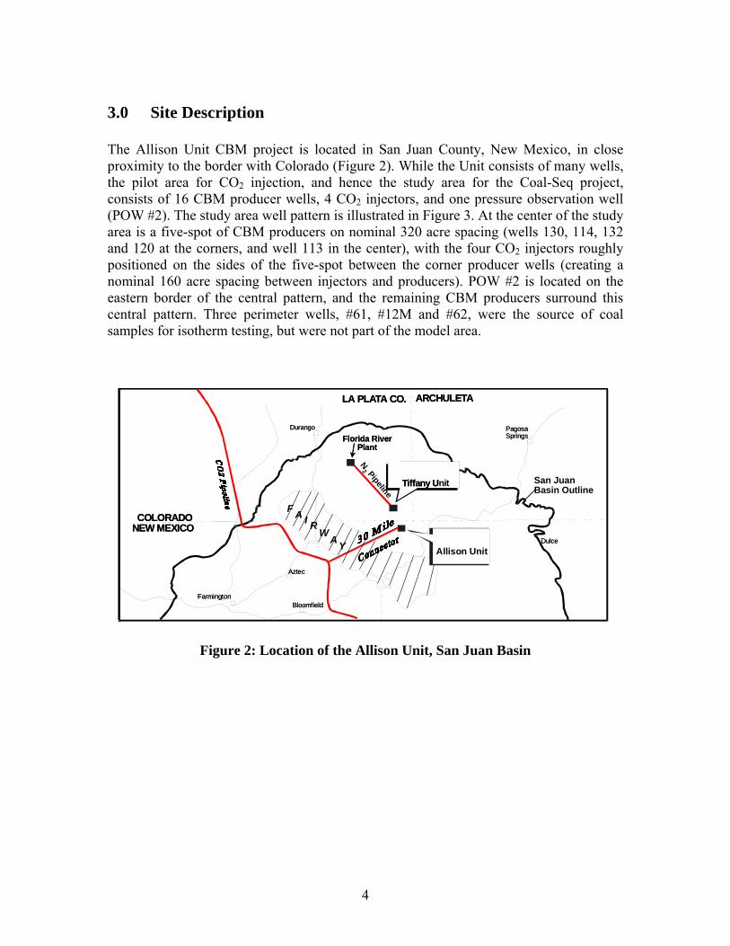
3.0 Site Description The Allison Unit CBM project is located in San Juan County, New Mexico, in close proximity to the border with Colorado (Figure 2). While the Unit consists of many wells, the pilot area for CO2 injection, and hence the study area for the Coal-Seq project, consists of 16 CBM producer wells, 4 CO2 injectors, and one pressure observation well (POW #2). The study area well pattern is illustrated in Figure 3. At the center of the study area is a five-spot of CBM producers on nominal 320 acre spacing (wells 130, 114, 132 and 120 at the corners, and well 113 in the center), with the four CO2 injectors roughly positioned on the sides of the five-spot between the corner producer wells (creating a nominal 160 acre spacing between injectors and producers). POW #2 is located on the eastern border of the central pattern, and the remaining CBM producers surround this central pattern. Three perimeter wells, #61, #12M and #62, were the source of coal samples for isotherm testing, but were not part of the model area.

Farmington

Aztec

Bloomfield

Dulce

Durango PagosaSprings

COLORADONEW MEXICO

LA PLATA CO. ARCHULETA

Allison Unit

F A I RW

A Y

Florida RiverPlant

Tiffany Unit San Juan Basin Outline

N2 Pipeline

Farmington

Aztec

Bloomfield

Dulc

Farmington

Aztec

Bloomfield

Dulce


COLORAD

e


COLORADONEW MEXICO


ONEW MEXICO


Allison Unit

F A I RW

A Y

Florida RiverPlant

Tiffany U

Florida RiverPlant

Tiffany Unit San Juan Basin Outline

N2 Pipeline

Figure 2: Location of the Allison Unit, San Juan Basin

5

Figure 3: Producer/Injector Well Pattern, Allison Unit

61

6

The producing history for the study area is shown in Figure 4. The field originally began production in 1989, with CO2 injection beginning in 1995. Injection was suspended in August 2001 to evaluate the results. Several points are worth pointing out regarding the producing history:

o Upon commencement of the injection operations, the five producer wells in the central five-spot pattern were shut in. The purpose was to facilitate CH4/CO2 exchange in the reservoir. After about six months, CO2 injection was suspended for about another six months, during which time the five shut-in producers were re-opened. These activities can be clearly identified in Figure 4; their impact on long-term production performance however, if any, is unclear.

o Shortly after CO2 injection began, a program of production

enhancement activities unrelated to the CO2-ECBM pilot was implemented. Those activities included well recavitations, well reconfigurations (conversion from tubing/packer completions to annular flow with a pump installed for well dewatering), line pressure reductions due to centralized compression, and also the installation of on-site compression. These activities largely coincided with the dramatic increase in production observed beginning in mid-1998.

These effects are illustrated for an individual well in Figure 5. In this case, the well was recavitated within a month of the start of CO2 injection. The line pressure reduction did not appear to immediately impact well performance due to the well configuration at the time (tubing flow). However once the well was reconfigured to annular flow with a dewatering pump, reduced line pressure was directly exposed to the producing coal seams in the annulus and production increased significantly. Production again increased when on-site compression was installed. One can easily appreciate the difficulty these operations create when attempting to isolate and understand the impact of CO2 injection on field performance. Hence a comprehensive reservoir simulation study, that accounts for each and every one of these events, was chosen to try to isolate and evaluate the impact of CO2 injection on field performance.

CO2 Source The CO2 being injected at Allison is sourced from natural CO2 reservoirs located in the Cortez area of New Mexico. CO2 from these reservoirs is delivered to West Texas for enhanced oil recovery projects via a high pressure pipeline, operated by Kinder Morgan, that runs through the San Juan basin. Burlington Resources constructed a 36 mile, 4-inch diameter spur from this main pipeline to the Allison Unit. CO2 is delivered from the pipeline at a pressure of approximately 2200 psi, and it is reduced to approximately 1500 psi, primarily due to friction, prior to injection.

7

Figure 4: Producing History, Allison Unit Study Area

Figure 5: Producing History, Individual Allison Unit Well

0

20000

40000

60000

80000

100000

120000

140000

160000

Jan-

89

Jul-8

9

Jan-

90

Jul-9

0

Jan-

91

Jul-9

1

Jan-

92

Jul-9

2

Jan-

93

Jul-9

3

Jan-

94

Jul-9

4

Jan-

95

Jul-9

5

Jan-

96

Jul-9

6

Jan-

97

Jul-9

7

Jan-

98

Jul-9

8

Jan-

99

Jul-9

9

Jan-

00

Jul-0

0

Jan-

01

Date

Rat

e

0

100

200

300

400

500

600

700

800

900

1000

Pres

sure

Gas, Mcf/mo

Csg Press, psi

Line Press, psi

Recavitate (5/95)

Well reconfigured, pump installed (3/99)

Line pressures reduced

Onsite compression installed

CO2 injection commencedreduced

0

20000

40000

60000

80000

100000

120000

140000

160000

Jan-

89

Jul-8

9

Jan-

90

Jul-9

0

Jan-

91

Jul-9

1

Jan-

92

Jul-9

2

Jan-

93

Jul-9

3

Jan-

94

Jul-9

4

Jan-

95

Jul-9

5

Jan-

96

Jul-9

6

Jan-

97

Jul-9

7

Jan-

98

Jul-9

8

Jan-

99

Jul-9

9

Jan-

00

Jul-0

0

Jan-

01

Date

Rat

e

0

100

200

300

400

500

600

700

800

900

1000

Pres

sure

Gas, Mcf/mo

Csg Press, psi

Line Press, psi

Recavitate (5/95)




CO2 injection commencedreduced

0

20000

40000

60000

80000

100000

120000

140000

160000

Jan-

89

Jul-8

9

Jan-

90

Jul-9

0

Jan-

91

Jul-9

1

Jan-

92

Jul-9

2

Jan-

93

Jul-9

3

Jan-

94

Jul-9

4

Jan-

95

Jul-9

5

Jan-

96

Jul-9

6

Jan-

97

Jul-9

7

Jan-

98

Jul-9

8

Jan-

99

Jul-9

9

Jan-

00

Jul-0

0

Jan-

01

Date

Rat

e

0

100

200

300

400

500

600

700

800

900

1000

Pres

sure

Gas, Mcf/mo

Csg Press, psi

Line Press, psi

Recavitate (5/95)




CO2 injection commenced Line pressures reduced

0

200,000

400,000

600,000

800,000

1,000,000

1,200,000

1,400,000

1,600,000

1,800,000

2,000,000

Jan-

89

Jul-8

9

Jan-

90

Jul-9

0

Jan-

91

Jul-9

1

Jan-

92

Jul-9

2

Jan-

93

Jul-9

3

Jan-

94

Jul-9

4

Jan-

95

Jul-9

5

Jan-

96

Jul-9

6

Jan-

97

Jul-9

7

Jan-

98

Jul-9

8

Jan-

99

Jul-9

9

Jan-

00

Jul-0

0

Jan-

01

Jul-0

1

Date

Rat

es, M

cf/m

o

0

500

1,000

1,500

2,000

2,500

3,000

3,500

4,000

Indi

vidu

al W

ell G

as R

ate,

Mcf

/d

Gas Rate, Mcf/moCO2 Injection Rate, Mcf/moWell Gas Rate, Mcf/d

16 producers, 4 injectors, 1 POW

Five wells shutin during initial injection period

Injection suspended, five wells reopened

Line pressures reduced, wells recavitated, wells reconfigured, onsite compression installed

Injection resumed

+/- 3 1/2 Mcfd

Peak @ +/- 57 MMcfd

8

The Allison Unit wells produce from three Upper Cretaceous Fruitland Formation coal seams, named the Yellow, Blue and Purple (from shallowest to deepest) using Burlington Resources’ terminology. A summary of basic coal depth, thickness, pressure and temperature information is provided in Table 1.

Table 1: Allison Unit Basic Coal Reservoir Data

In general, the wells are top-set above the coal intervals with 7-inch casing cemented into place. The coal intervals were then drilled with a 6-1/4 inch bit with water to below the deepest target coal (Purple). The coals were then cavitated and 5-1/2 inch perforated liners installed without cement. The wells were then configured for commingled gas/water production up the tubing. In the case of the CO2 injection wells, the wells were drilled to total depth, and 5-1/2 inch casing run and cemented into place. The coal intervals were then perforated, and perforation breakdown treatments performed. The coal intervals in the injection wells did not receive massive stimulation treatments to prevent possible communication pathways being created into bounding non-coal layers. The downhole configuration for injection wells consists of a tubing and packer arrangement, however the internal surface of the tubing is coated with fiberglass to prevent corrosion. In addition, the CO2 is heated to approximately reservoir temperature prior to injection to prevent expansion/contraction of the well tubulars during suspension periods.

3100 feet

3 (Yellow, Blue, Purple)

43 feetYellow – 22 ft

Blue – 10 ftPurple – 11 ft

1650 psi

120°F

Average Depth to Top Coal

Average Total Net Thickness

Initial Pressure

Temperature

ValueProperty

3100 feet

3 (Yellow, Blue, Purple)

43 feetYellow – 22 ft

Blue – 10 ftPurple – 11 ft

1650 psi

120°F

Average Depth to Top Coal

Average Total Net Thickness

Initial Pressure

Temperature

Number of Coal Intervals

ValueProperty

9

4.0 Reservoir Description Structure contour and isopach maps of each coal and interburden horizon were constructed based on lithologic picks made by Burlington Resources. A sample structure map for the Yellow coal is presented in Figure 6, and the total net coal isopach is presented in Figure 7. A gentle dip in the area exists towards the south-southwest, where the coals also thicken slightly.

Figure 6: Structure Map, Yellow Coal (units in feet above sea level)

Figure 7: Total Net Coal Isopach, Allison Unit Study Area (units in feet)

900000 902000 904000 906000 908000 910000 912000 914000 916000 918000

13422000

13424000

13426000

13428000

13430000

13432000

13434000

13436000

13438000

112

115

121

131140

141

142

143

113

114

120

130

132

12M

61

62

101

102

104

106

108

111

119

POW #2

105

118

122

146

900000 902000 904000 906000 908000 910000 912000 914000 916000 918000

13422000

13424000

13426000

13428000

13430000

13432000

13434000

13436000

13438000

112

115

121

131140

141

142

143

113

114

120

130

132

12M

61

62

101

102

104

106

108

111

119

POW #2

105

118

122

146

10

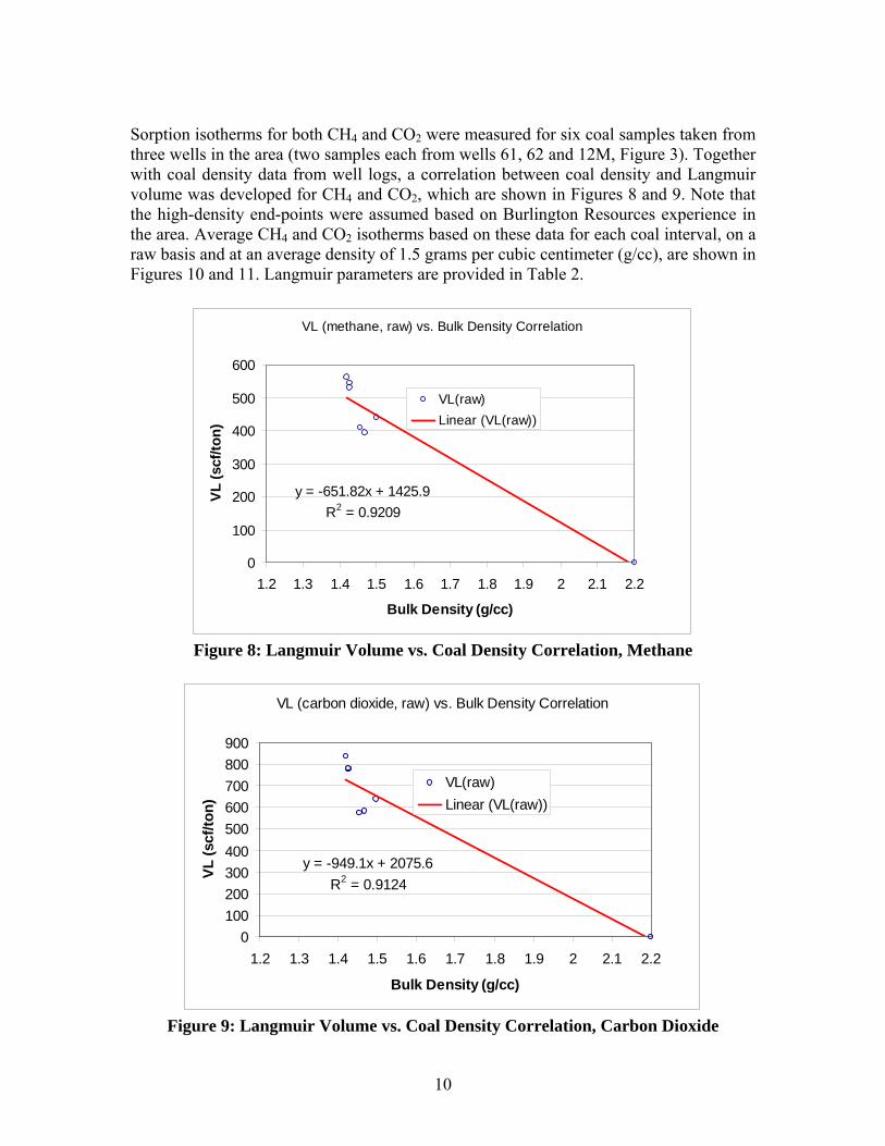
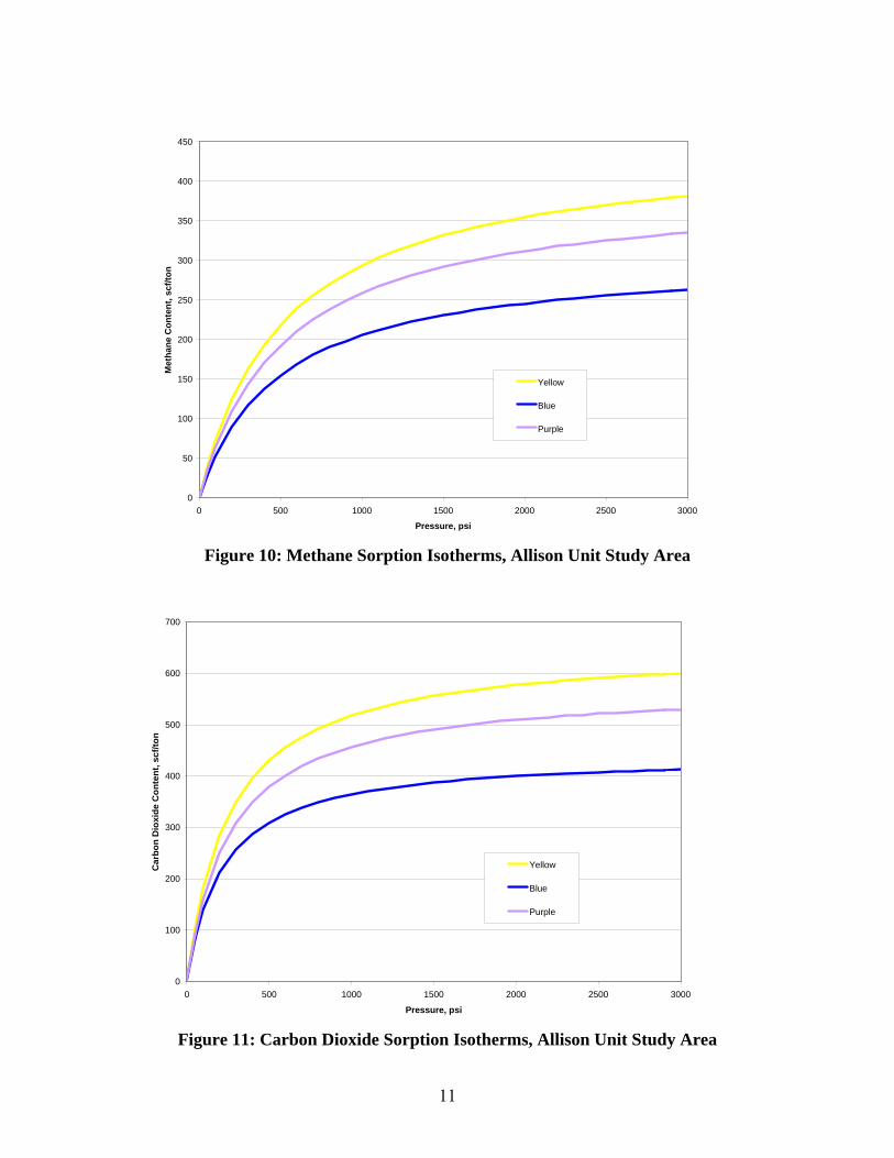
Sorption isotherms for both CH4 and CO2 were measured for six coal samples taken from three wells in the area (two samples each from wells 61, 62 and 12M, Figure 3). Together with coal density data from well logs, a correlation between coal density and Langmuir volume was developed for CH4 and CO2, which are shown in Figures 8 and 9. Note that the high-density end-points were assumed based on Burlington Resources experience in the area. Average CH4 and CO2 isotherms based on these data for each coal interval, on a raw basis and at an average density of 1.5 grams per cubic centimeter (g/cc), are shown in Figures 10 and 11. Langmuir parameters are provided in Table 2.

VL (methane, raw) vs. Bulk Density Correlation

y = -651.82x + 1425.9R2 = 0.9209

0

100

200

300

400

500

600

1.2 1.3 1.4 1.5 1.6 1.7 1.8 1.9 2 2.1 2.2

Bulk Density (g/cc)

VL (s

cf/to

n)

VL(raw)Linear (VL(raw))

Figure 8: Langmuir Volume vs. Coal Density Correlation, Methane

VL (carbon dioxide, raw) vs. Bulk Density Correlation

y = -949.1x + 2075.6R2 = 0.9124

0100200300400500600700800900

1.2 1.3 1.4 1.5 1.6 1.7 1.8 1.9 2 2.1 2.2

Bulk Density (g/cc)

VL (s

cf/to

n)

VL(raw)Linear (VL(raw))

Figure 9: Langmuir Volume vs. Coal Density Correlation, Carbon Dioxide

11

0

50

100

150

200

250

300

350

400

450

0 500 1000 1500 2000 2500 3000

Pressure, psi

Met

hane

Con

tent

, scf

/ton

Yellow

Blue

Purple

Figure 10: Methane Sorption Isotherms, Allison Unit Study Area

0

100

200

300

400

500

600

700

0 500 1000 1500 2000 2500 3000

Pressure, psi

Car

bon

Dio

xide

Con

tent

, scf

/ton

Yellow

Blue

Purple

Figure 11: Carbon Dioxide Sorption Isotherms, Allison Unit Study Area

12

Table 2: Langmuir Constants, by Layer

Carbon Dioxide Methane

VL SCF/ton(ft3/ft3)

PL, psi

VL SCF/ton(ft3/ft3)

PL, psi

Yellow 652 (30.5) 259 448 (21.0) 525 Blue 443 (23.8) 216 305 (16.4) 484 Purple 576 (28.4) 261 393 (19.4) 519 Using coal density maps generated for each coal seam, based on log-derived coal density data, Langmuir volume (VL) maps were created for each coal layer. During this procedure, consistency was established between the density basis for the core analysis and log results. Interestingly, it was found that little variation in Langmuir volume occurred within a given coal layer (when converted to units of volume/volume), but considerable variations existed from layer to layer. Table 3 summarizes these results, and their implication to methane resource distribution.

Table 3: Layer Sorption Properties and Distribution of Methane Resource

11

10

22

Average Thickness (ft)

26%1.58393Purple

19%1.72305Blue

55%1.50448Yellow

Gas-in-placeLog

Density(g/cc)

VL(scf/ton)

Zone

11

10

22

Average Thickness (ft)

26%1.58393Purple

19%1.72305Blue

55%1.50448Yellow

Gas-in-placeLog

Density(g/cc)

VL(scf/ton)

Zone

13

Relative permeability curves were derived for the field using a novel procedure developed by Burlington Resources. The procedure involves the following steps:

1. Estimate initial mobile water in place by performing decline curve analysis on water production for each well.

2. Compute effective water permeability versus time using Darcy’s Law and

accounting for reservoir pressure depletion via material balance.

3. Use water material balance to calculate mobile water saturation versus time.

4. Plot effective water permeability versus mobile water saturation.

5. Repeat steps 2 & 3 for gas.

6. Plot the ratio of effective water permeability to effective gas permeability versus mobile water saturation.

7. Adjust the absolute value of mobile water saturation for each well until the curves

developed in step 5 approximately overlie each other.

8. Determine actual porosity by assuming a residual water saturation.

9. Adjust relative permeability curves accordingly. This procedure, while requiring considerable judgment, yields both a relative permeability relationship for the entire field, as well as a distribution of porosity across the field. When applied to Allison, the relative permeability curves (after curve-fitting) and porosity maps that resulted are presented in Figures 12 and 13 respectively (assuming a residual water saturation of zero). Note that the right-hand portion of the water relative permeability curve in Figure 12 was smoothed to facilitate more stable reservoir modeling. Porosity values ranged from a high of 0.3% in the southwest to as low as 0.05% in the northwest.

Figure 12: Relative Permeability Curves, Allison Unit

Relative Permeability Curves

0.0000

0.2000

0.4000

0.6000

0.8000

1.0000

0% 20% 40% 60% 80% 100%

Water Saturation

Relat

ive P

erm

eabi

lity WaterGas

Smoothed

14

900000 902000 904000 906000 908000 910000 912000 914000 916000 918000

13422000

13424000

13426000

13428000

13430000

13432000

13434000

13436000

13438000

112

115

121

131140

141

142

143

113

114

120

130

132

12M

61

62

101

102

104

106

108

111

119

POW #2

105

118

122

146

900000 902000 904000 906000 908000 910000 912000 914000 916000 918000

13422000

13424000

13426000

13428000

13430000

13432000

13434000

13436000

13438000

112

115

121

131140

141

142

143

113

114

120

130

132

12M

61

62

101

102

104

106

108

111

119

POW #2

105

118

122

146

Figure 13: Porosity Map, Allison Unit (units in fractions)

A comparison was made between the relative permeability curves derived here and others, both laboratory and simulator derived, from the San Juan Basin3. That comparison is shown in Figure 14, and suggests that these curves are markedly different, and more “conservative” for gas flow, than even the laboratory-derived results.

0.001

0.01

0.1

1

10

100

1000

0 0.2 0.4 0.6 0.8 1

Sw

Krg

/Krw

Sample 7 Core B/Coal Site Hamilton No. 3 Cause 112-73

Tiffany Coal Site Allison

Allison Curve

Laboratory CurvesHistory-Match Curves

0.001

0.01

0.1

1

10

100

1000

0 0.2 0.4 0.6 0.8 1

Sw

Krg

/Krw

Sample 7 Core B/Coal Site Hamilton No. 3 Cause 112-73

Tiffany Coal Site Allison

Allison Curve

Laboratory CurvesHistory-Match Curves

Figure 14: Comparison of Relative Permeability Curves

15

In May, 2000, pressure buildup tests were performed on 12 wells in the Allison Unit, eight of which were inside the study area. Pressure data were collected at the surface. Analysis of the data provided estimates of effective gas permeability, skin factor, and reservoir pressure. Two adjustments of the results were made to 1) derive absolute permeability from the effective gas permeability results and 2) correct to initial conditions – accounting for both pressure-dependent permeability and matrix shrinkage. For the first correction, the following procedure was used:

1. Estimate effective permeability to water just prior to shut-in using Darcy’s Law. 2. Compute the ratio of effective water permeability to effective gas permeability.

3. For that ratio, lookup the corresponding relative permeability to gas based on

the relative permeability curves developed for the field.

4. Compute absolute permeability based on effective gas permeability and relative gas permeability at that point in time.

This procedure was applied to for each well for which data was available, and the correlation was developed between the “measured” effective gas permeability and “corrected” absolute permeability. That correlation is provided in Figure 15.

Figure 15: Correlation between Effective Gas and Absolute Permeability

Keg vs Kabs

y = 1.984x + 12.138R2 = 0.8691

0.020.040.060.080.0

100.0120.0140.0160.0180.0

0 20 40 60 80

Keg, md

Kab

s, m

d

16

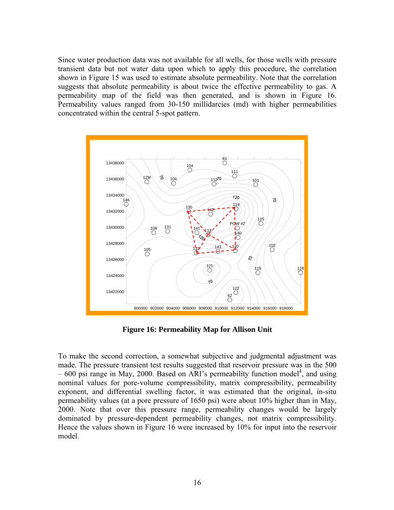
Since water production data was not available for all wells, for those wells with pressure transient data but not water data upon which to apply this procedure, the correlation shown in Figure 15 was used to estimate absolute permeability. Note that the correlation suggests that absolute permeability is about twice the effective permeability to gas. A permeability map of the field was then generated, and is shown in Figure 16. Permeability values ranged from 30-150 millidarcies (md) with higher permeabilities concentrated within the central 5-spot pattern.

112

115

121

131140

141

142

143

113

114

120

130

132

12M

61

62

101

102

104

106

108

111

119

POW #2

105

118

122

146

900000 902000 904000 906000 908000 910000 912000 914000 916000 918000

13422000

13424000

13426000

13428000

13430000

13432000

13434000

13436000

13438000

Figure 16: Permeability Map for Allison Unit To make the second correction, a somewhat subjective and judgmental adjustment was made. The pressure transient test results suggested that reservoir pressure was in the 500 – 600 psi range in May, 2000. Based on ARI’s permeability function model4, and using nominal values for pore-volume compressibility, matrix compressibility, permeability exponent, and differential swelling factor, it was estimated that the original, in-situ permeability values (at a pore pressure of 1650 psi) were about 10% higher than in May, 2000. Note that over this pressure range, permeability changes would be largely dominated by pressure-dependent permeability changes, not matrix compressibility. Hence the values shown in Figure 16 were increased by 10% for input into the reservoir model.

17

A final step in the reservoir characterization process was to estimate the variables that control changes in permeability as a function of pressure and gas concentration. Specifically, these variables are pore volume compressibility-Cp; matrix compressibility-Cm; and differential swelling factor-Ck. The formulas relating coal permeability to these parameters are:

( )[ ] ( ) ( )[ ]CCCCCCP

CPPC tkii

imiipi −+−

∆∆

−−−−= )(11 φφφ

Pressure-Dependent Term Concentration-Dependent Term and

n

i

k )(φφ

=

Note that the terminology is defined in the Nomenclature (Section 13). To estimate these parameters, the results of injection/falloff tests performed in the four CO2 injection wells, performed in August 2001 (when they were shut-in), were utilized. Those tests suggested that coal permeability values in the regions near the injector wells, and hence heavily influenced by CO2, were <1 md. Using the estimated initial in-situ permeability values as estimated from the permeability map shown in Figure 16, and the values determined from the August 2001 injection/falloff tests (as well as the prevailing reservoir pressure at that time) the variables for the permeability function model were estimated using the analytic model presented above. The resulting values are presented in Table 4.

Table 4: Estimated Permeability Function Parameters

Well No.

Porosity*

Cp (x10-6) (1/psi)

Cm (x10-6) (1/psi)

Ck

140

0.23% 200 1 1.25

141

0.16% 200 1 1.10

142

0.17% 200 1 1.15

143

0.25% 200 1 1.20

*from porosity map

18

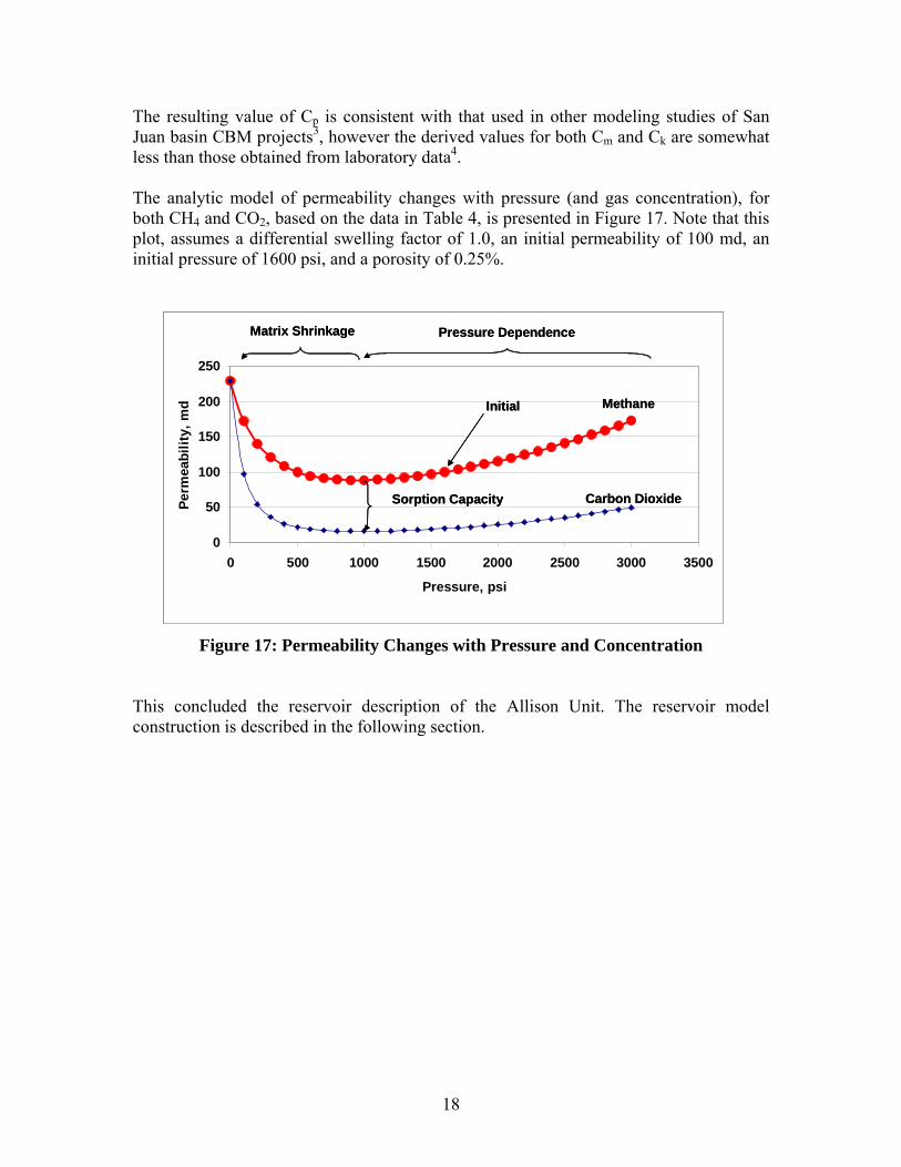
The resulting value of Cp is consistent with that used in other modeling studies of San Juan basin CBM projects3, however the derived values for both Cm and Ck are somewhat less than those obtained from laboratory data4. The analytic model of permeability changes with pressure (and gas concentration), for both CH4 and CO2, based on the data in Table 4, is presented in Figure 17. Note that this plot, assumes a differential swelling factor of 1.0, an initial permeability of 100 md, an initial pressure of 1600 psi, and a porosity of 0.25%.

Figure 17: Permeability Changes with Pressure and Concentration This concluded the reservoir description of the Allison Unit. The reservoir model construction is described in the following section.

0

50

100

150

200

250

0 500 1000 1500 2000 2500 3000 3500

Pressure, psi

Perm

eabi

lity,

md Methane

Carbon Dioxide

Initial

Matrix Shrinkage Pressure Dependence

Sorption Capacity

0

50

100

150

200

250

0 500 1000 1500 2000 2500 3000 3500

Pressure, psi

Perm

eabi

lity,

md Methane

Carbon Dioxide

Initial


Sorption Capacity

Methane

Carbon Dioxide

Initial


Sorption Capacity

19

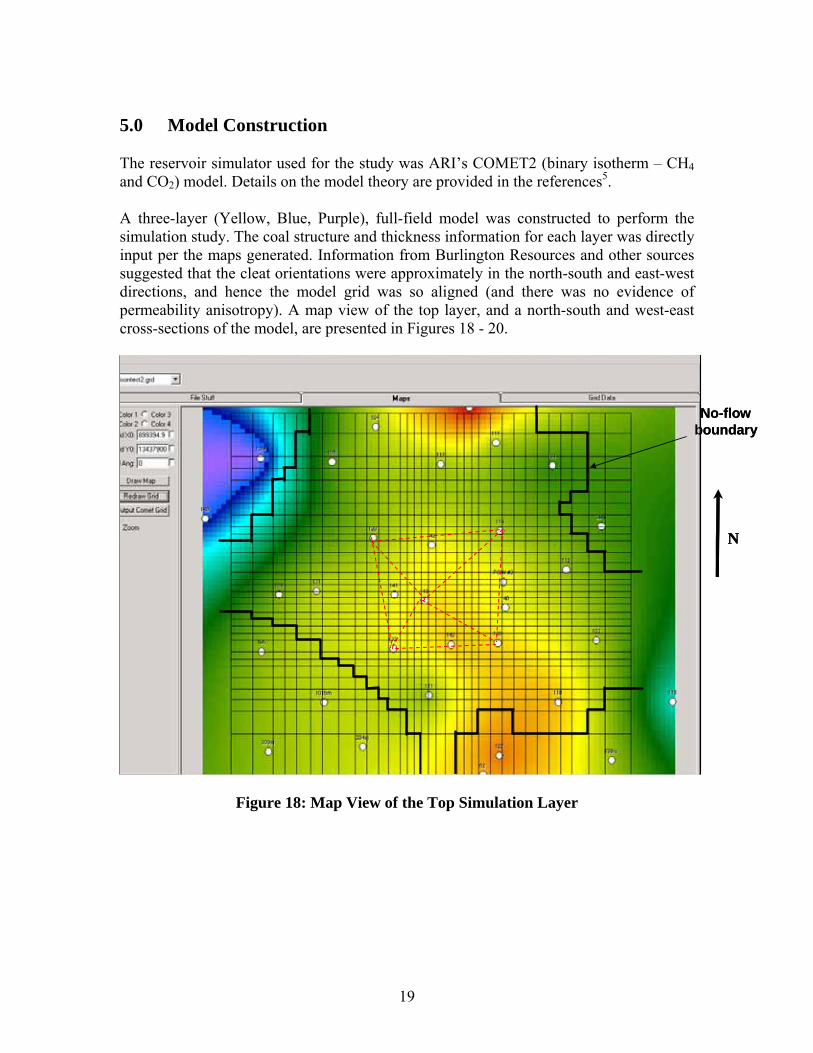
5.0 Model Construction The reservoir simulator used for the study was ARI’s COMET2 (binary isotherm – CH4 and CO2) model. Details on the model theory are provided in the references5. A three-layer (Yellow, Blue, Purple), full-field model was constructed to perform the simulation study. The coal structure and thickness information for each layer was directly input per the maps generated. Information from Burlington Resources and other sources suggested that the cleat orientations were approximately in the north-south and east-west directions, and hence the model grid was so aligned (and there was no evidence of permeability anisotropy). A map view of the top layer, and a north-south and west-east cross-sections of the model, are presented in Figures 18 - 20.

Figure 18: Map View of the Top Simulation Layer

N

PDS090401.ppt

No-flow boundary

N

PDS090401.ppt

No-flow boundary

20

Figure 19: North-South Cross Section of the Simulation Model

Figure 20: West-East Cross Section of the Simulation Model

21

The model gridblock dimensions were 33 x 32 x 3 (approximately 3,200 total grid blocks, 2,600 of which were active), representing an area of about 7,100 acres. The corners of the model were isolated using no-flow barriers to account for producing wells immediately adjacent to these portions of the study area. The Langmuir volume and pressure values were constant for each layer, but varied for each layer based on Table 2. The porosity map presented in Figure 13 was used for all layers. However, a minimum porosity value of 0.15% was imposed – lower values of porosity were judged to be unreasonable. The permeability of each layer was per the map presented in Figure 16, but with the values increased by 10% as explained in the previous discussion. Other relevant reservoir parameters are presented in Table 5.

Table 5: Reservoir Parameters used in Simulation Model Parameter Value Source Remarks

Initial Pressure Reservoir Temperature Initial Water Saturation Initial Gas Content Sorption Time Fracture Spacing Gas Composition Relative Permeability Perm Function Parameters

1650 psi 120º F 95%

Per Isotherm 10 days 1 inch

95.5% CH4, 4.5% CO2 Figure 12 Table 4*

Burlington Burlington Assumed Assumed Assumed Assumed

Gas Composition Measurement

Independent Analysis Independent Analysis

~0.53 psi/ft

Equilibrium value Same for CH4 & CO2

* Note: A differential swelling factor of 1.0 was adopted for the model.

Additionally, well completion and operating parameters were examined for input into the model. This was particularly important given the complexity of the field history, and the desire to isolate and study the effects of CO2 injection. First, to account for the recavitation operations in the producing wells, the procedure presented below was adopted. This procedure assumes that the well producing pressure before and after the restimulation treatment did not change significantly (i.e., well operating practices did not substantially change before/after the recavitation treatment), and that the entire effect of the treatment should be reflected in the gas rate.

1. Compile the computed skin factors based on the May, 2000 pressure transient tests. Where actual values were not available, assume an average value. Since all recavitation treatments were performed prior to May, 2000, the skin values derived from the well tests performed at that time represent the post-recavitation values for skin factor.

22

2. Determine the actual gas production immediately preceding and following the recavitation operations from the production history data. Compute the folds-of-increase in production resulting from the operation.

3. Using conventional flow theory, compute the change in skin factor required to

achieve the production response observed, assuming all other parameters remain unchanged.

4. By taking the post-recavitation skin, and the computed change in skin, compute

the pre-recavitation skin factor. The results of applying this procedure are presented in Table 6. Note that in the model a maximum constraint for pre-recavitation skin factor of +10 was imposed.

Table 6: Estimated Skin Factor Changes Due to Recavitation

For the injector wells, skin factor values determined from the August, 2001 injection/falloff tests were used. These values were in the –2 to –4 range, and are believed reasonable since the CO2 injection pressures were close to the fracturing pressure of the coals (2,300 – 2,500 psi bottomhole pressure at a depth of about 3,100 feet – a pressure gradient of about 0.77 psi/ft). Finally, based on well completion records, producer well #106 was not completed in the Purple horizon, and injector well #143 was not completed in the Yellow horizon.

130 130

23

6.0 Initial Model Results The independent parameter used for the reservoir model was gas production (and injection) rate to maintain material balance, and the dependent (history match) parameters were water production rate, flowing pressures (producing and injecting), and gas composition. Note that only some of these data were available for some periods for some wells; whatever was available was used. In addition, the pressure history at POW #2 was available, as were the reservoir pressures at some of the producing wells in May 2000 based on the pressure transient tests. A comparison of the actual versus model field gas rate is presented in Figure 21. A complete set of plots comparing the initialization run results to the actual data are provided in Appendix A. The only conclusion that can be derived from this result, since the model was “driven” on gas rate, is that model (as initially constructed) was capable of delivering the gas volumes required. (However, it should be noted that one well - #119 – was not achieving the required gas rate towards the end of the simulation period.)

Actual

Simulated

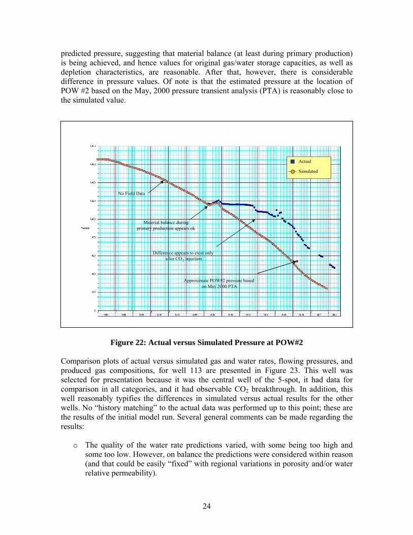
Figure 21: Actual versus Simulated Field Gas Rate The actual versus model pressure at POW#2 for the initial simulation run is presented in Figure 22. Actual pressure data is only available after the commencement of CO2 injection. At that time, there appears to be excellent agreement between actual and

24

predicted pressure, suggesting that material balance (at least during primary production) is being achieved, and hence values for original gas/water storage capacities, as well as depletion characteristics, are reasonable. After that, however, there is considerable difference in pressure values. Of note is that the estimated pressure at the location of POW #2 based on the May, 2000 pressure transient analysis (PTA) is reasonably close to the simulated value.

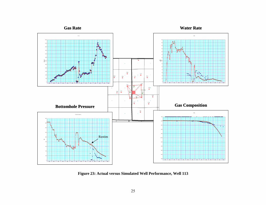
Figure 22: Actual versus Simulated Pressure at POW#2 Comparison plots of actual versus simulated gas and water rates, flowing pressures, and produced gas compositions, for well 113 are presented in Figure 23. This well was selected for presentation because it was the central well of the 5-spot, it had data for comparison in all categories, and it had observable CO2 breakthrough. In addition, this well reasonably typifies the differences in simulated versus actual results for the other wells. No “history matching” to the actual data was performed up to this point; these are the results of the initial model run. Several general comments can be made regarding the results:

o The quality of the water rate predictions varied, with some being too high and some too low. However, on balance the predictions were considered within reason (and that could be easily “fixed” with regional variations in porosity and/or water relative permeability).

Actual

Simulated

No Field Data

Material balance duringprimary production appears ok

Difference appears to exist onlyafter CO2 injection

Approximate POW#2 pressure basedon May 2000 PTA

25

Water Rate

Gas CompositionBottomhole Pressure

Restim

Gas Rate Water Rate

Gas CompositionBottomhole Pressure

Restim

Gas Rate

Figure 23: Actual versus Simulated Well Performance, Well 113

26

o In all cases, the predicted bottomhole flowing pressures were higher than the

measured values – which were actually surface casing pressure data – usually by 200-300 psi. While some difference might be expected due to the different types of data being compared (surface vs. downhole), the magnitude of the difference seems large. (The wells are believed to be pumped-off with little water head existing above the coal seam.) In most cases the predicted flowing pressures appear smooth through the period when the recavitation operations were performed. This result was per the model design.

o In general, the trend in gas composition was reasonably well replicated. Note that

due to limitations of the COMET2 model, gas composition could not be changed regionally in the model (an average value across the field is used). Hence one must examine the degree to which the prediction and data are parallel to each other, understanding that each would have to be calibrated to a different regional base-case composition. In some cases (most noteworthy well #113), the increase in CO2 content of the produced gas occurs more rapidly than that actually observed.

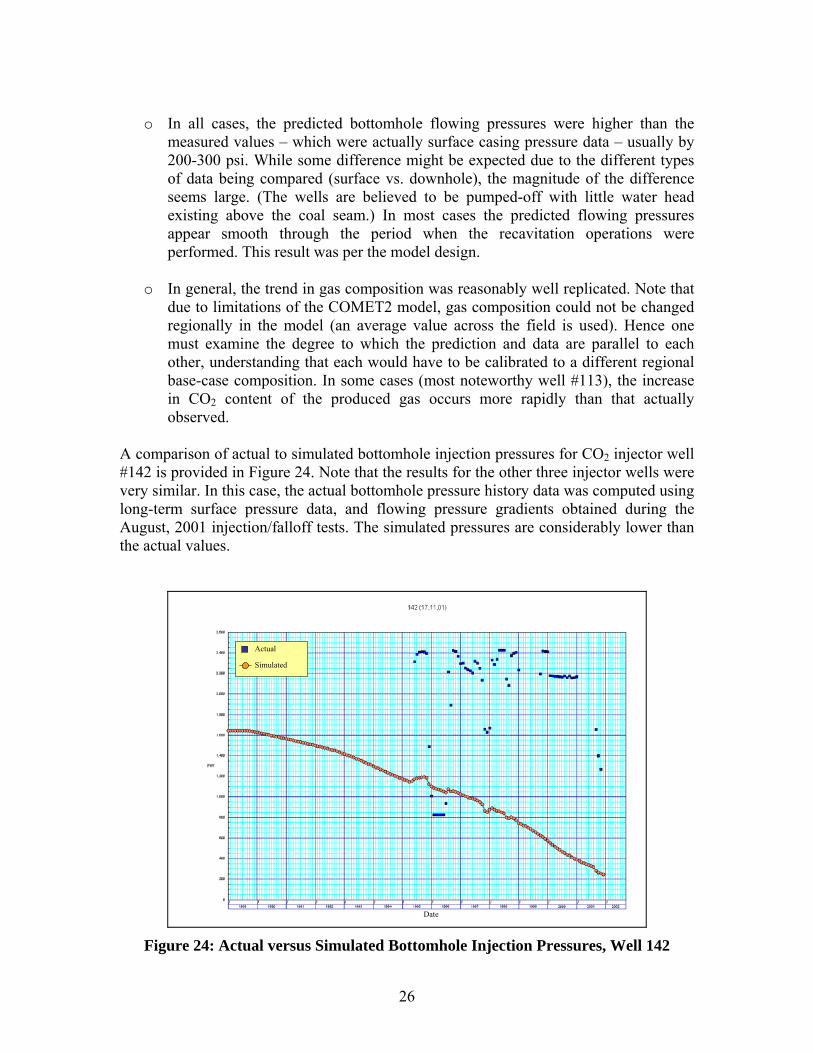
A comparison of actual to simulated bottomhole injection pressures for CO2 injector well #142 is provided in Figure 24. Note that the results for the other three injector wells were very similar. In this case, the actual bottomhole pressure history data was computed using long-term surface pressure data, and flowing pressure gradients obtained during the August, 2001 injection/falloff tests. The simulated pressures are considerably lower than the actual values.

Actual

Simulated

Date

Actual

Simulated

Date

Figure 24: Actual versus Simulated Bottomhole Injection Pressures, Well 142

27

7.0 History Matching The primary objective of this study was to generally calibrate this reservoir model to the field observations at Allison to better understand the CO2-ECBM sequestration process in coalseams. As such, the focus of history-matching was to make “global” adjustments to reservoir properties and observe if they better replicated overall field behavior. It was not the intention of this effort to make regional adjustments to reservoir properties purely for the sake of achieving a match, without independent technical evidence to justify such changes. As such, the history-matching process involved on varying a selected number of key inputs known to significantly affect field performance, and observe what overall effect they had on match quality. Those key inputs were:

o Permeability, including the absolute value, the functions that control pressure - and concentration – dependent variations, and relative permeability.

o Sorption behavior, including isotherm character and sorption time, for both methane and CO2.

7.1 Permeability The first and most obvious strategy to close the gap between simulated and actual producing/injecting pressures was to reduce coal permeability. However, reductions could only be performed to the point where gas production rate from the model could not be maintained to match the actual rates. To test the impact of lower permeability, permeability was decreased to 10% of the original value (an extreme case). Several noteworthy observations can be made from this scenario:

o The gas production rate in the model could not be sustained to match actual rates (Figure 25). By inference, the simulated bottomhole flowing pressures in many of the producing wells was now too low, rather than too high.

o Next, even at this level of reduced permeability, while improved over the initial

case the predicted injection well pressures were still much too low (Figure 26).

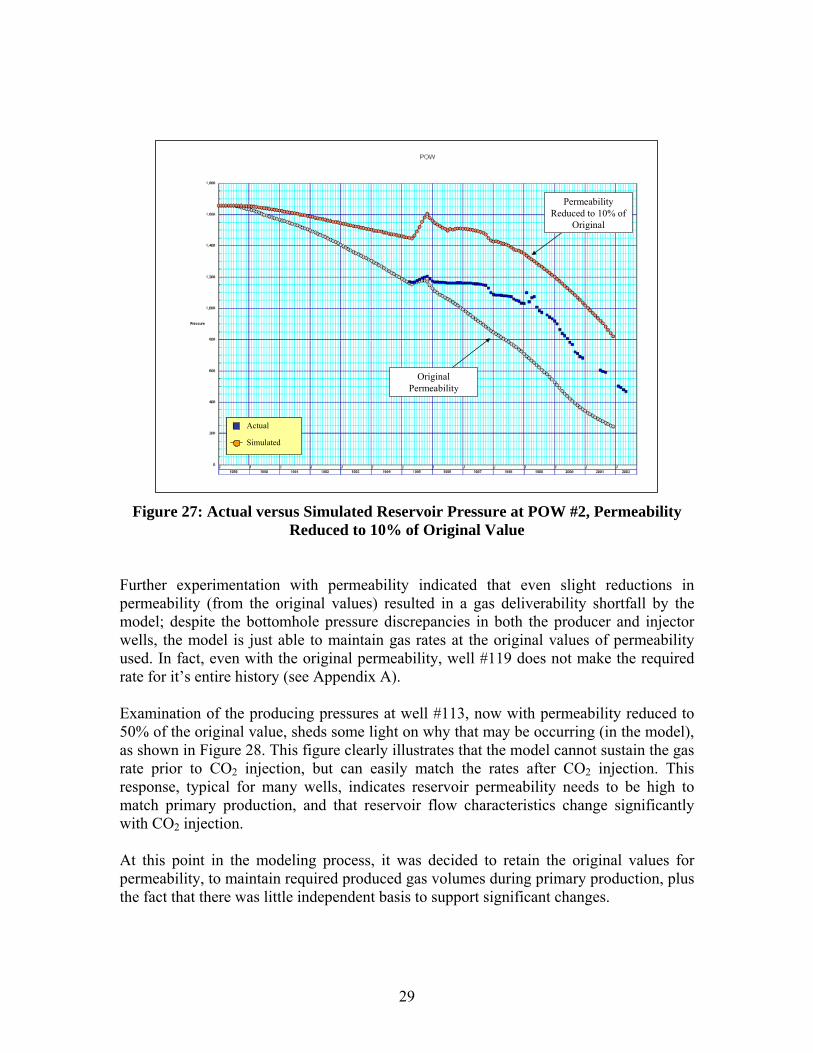
o The trends in reservoir pressure at POW #2 were much better replicated with the low permeability (Figure 27), albeit with values that are too high (material balance error).

28

Permeability Reduced to 10% of

Original

Original Permeability

Actual

Simulated


Original


Actual

Simulated

Actual

Simulated

Figure 25: Actual versus Simulated Field Gas Rate, Permeability Reduced to 10%

of Original Value


Actual

Simulated


Original


Actual

Simulated

Actual

Simulated


Original

Figure 26: Actual versus Simulated Bottomhole Pressure for Injector #142,

Permeability Reduced to 10% of Original Value

29


Actual

Simulated


Original


Actual

Simulated

Actual

Simulated


Original

Figure 27: Actual versus Simulated Reservoir Pressure at POW #2, Permeability

Reduced to 10% of Original Value Further experimentation with permeability indicated that even slight reductions in permeability (from the original values) resulted in a gas deliverability shortfall by the model; despite the bottomhole pressure discrepancies in both the producer and injector wells, the model is just able to maintain gas rates at the original values of permeability used. In fact, even with the original permeability, well #119 does not make the required rate for it’s entire history (see Appendix A). Examination of the producing pressures at well #113, now with permeability reduced to 50% of the original value, sheds some light on why that may be occurring (in the model), as shown in Figure 28. This figure clearly illustrates that the model cannot sustain the gas rate prior to CO2 injection, but can easily match the rates after CO2 injection. This response, typical for many wells, indicates reservoir permeability needs to be high to match primary production, and that reservoir flow characteristics change significantly with CO2 injection. At this point in the modeling process, it was decided to retain the original values for permeability, to maintain required produced gas volumes during primary production, plus the fact that there was little independent basis to support significant changes.

30


Original


Actual

Simulated


Original

Original Permeability Permeability

Reduced to 50% of Original


Actual

Simulated

Actual

Simulated

Figure 28: Actual versus Simulated Producing Pressure for Well #113, Permeability

Reduced to 50% of Original Value Next, attempts were made to improve the history-match by adjusting the functions that control pressure- and concentration-dependent permeability (specifically pore-volume compressibility and matrix compressibility), as well as relative permeability. After considerable experimentation with these variables, improvements in the match could not be achieved. As a result, while many different strategies related to permeability were tested to achieve a better history match, none provided that result in a satisfactory manner. Thus no changes were made to the initial model in this respect. Having stated that however, it is worth noting that the model appears to provide a reasonable replication of field behavior through the period of primary production, as indicated by material balance (pressure) match for POW#2 at the end of that period (Figure 22), and only after CO2 injection do things change significantly. 7.2 Sorption Behavior There is evidence based on laboratory studies performed as part of the Coal-Seq project that extrapolating single-component isotherm data to multi-component situations cannot be done very accurately, regardless of the sorption model used (i.e., extended Langmuir, equations of state, etc.)6. In addition, there is no explicit accounting for bi-directional diffusion in the coal matrix (i.e., CO2 going in and CH4 coming out) within COMET (or any other reservoir model that we are aware of). These factors may have something to do with the difficulty in achieving a match, and can be (at least crudely) investigated by

31

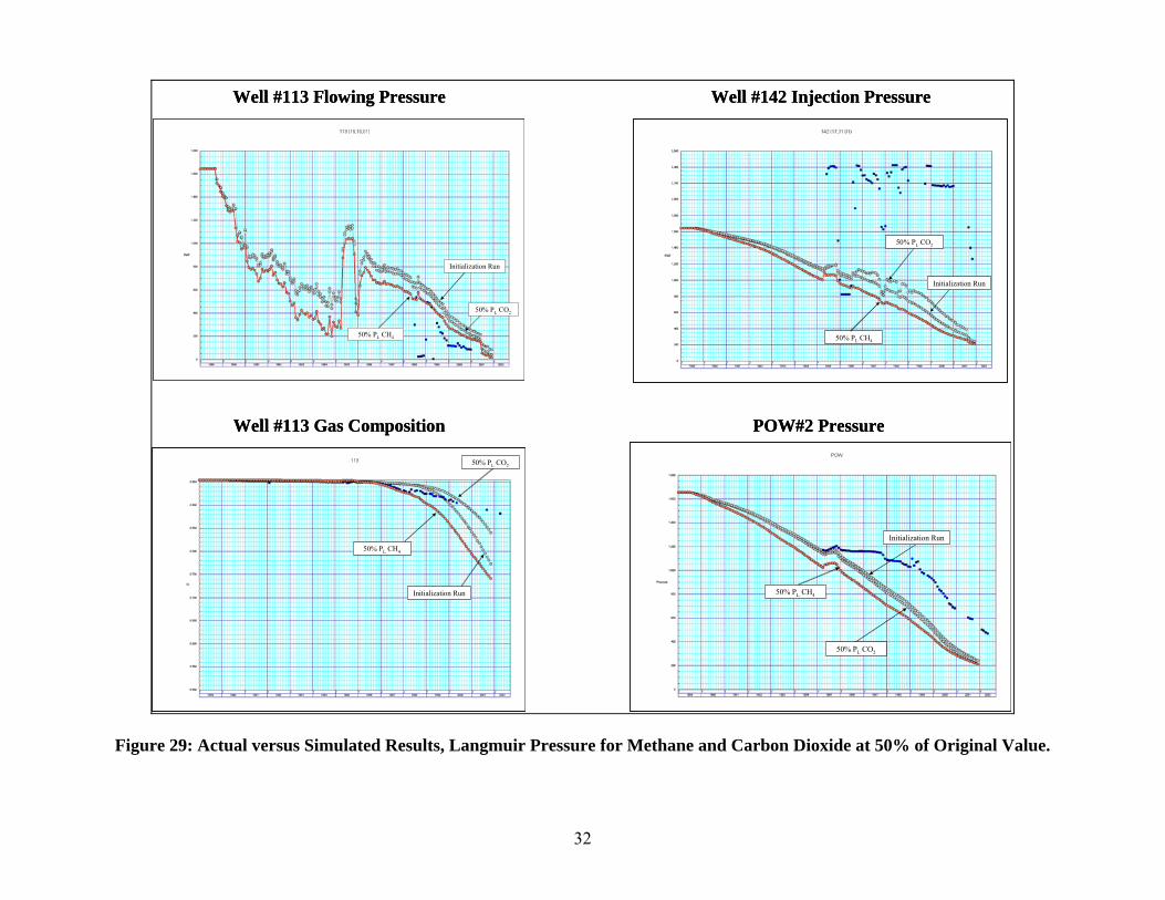
making changes to the coal sorption properties, specifically the Langmuir parameters and sorption time. The first sensitivity performed in this regard looked at decreasing (by 50%) the Langmuir pressure for each methane and carbon dioxide. This would cause either gas to require more pressure to adsorb/desorb a similar volume compared to the initial isotherm, and hence simulates a heightened “resistance” to diffusion resulting from bi-directional flow. The results for pressure at POW#2, flowing bottomhole pressure at well #113, gas composition at well #113, and injection pressure at well #142 are shown in Figure 29.

32

Well #113 Gas Composition

Well #113 Flowing Pressure

POW#2 Pressure

Well #142 Injection Pressure

50% PL CH4

50% PL CO2

Initialization Run

50% PL CH4

50% PL CO2

Initialization Run

50% PL CH4

50% PL CO2

Initialization Run

50% PL CH4

50% PL CO2

Initialization Run

Initialization Run

50% PL CH4

50% PL CO2

Initialization Run

50% PL CH4

50% PL CO2

50% PL CO2

50% PL CH4

Initialization Run

50% PL CO2

50% PL CH4

Initialization Run

Well #113 Gas Composition

Well #113 Flowing Pressure

POW#2 Pressure

Well #142 Injection Pressure

50% PL CH4

50% PL CO2

Initialization Run

50% PL CH4

50% PL CO2

Initialization Run

50% PL CH4

50% PL CO2

Initialization Run

50% PL CH4

50% PL CO2

Initialization Run

Initialization Run

50% PL CH4

50% PL CO2

Initialization Run

50% PL CH4

50% PL CO2

50% PL CO2

50% PL CH4

Initialization Run

50% PL CO2

50% PL CH4

Initialization Run

Figure 29: Actual versus Simulated Results, Langmuir Pressure for Methane and Carbon Dioxide at 50% of Original Value.

33

The results are very interesting. First, a pressure discrepancy becomes evident at POW#2 when the methane Langmuir pressure is reduced. This suggests that the original isotherm is a reasonable representation of reservoir conditions for the primary production period. However, after CO2 injection, the results in terms of flowing bottomhole pressures and gas composition at well #113 are improved with a reduced Langmuir pressure for methane. Further, the reduced carbon dioxide Langmuir pressure appears to also improve the injection pressure profile at well #142. These results again suggest that the original sorption isotherms appear reasonable for the primary production period, but the flow behavior changes when CH4 and CO2 mix in the reservoir, those changes being possibly related to binary sorption and/or diffusion A sensitivity run was also made varying sorption time, but significant changes in the original results were not observed. Therefore, similar to the result with permeability variations, it was decided to retain the original sorption properties in the model, since they seem to replicate primary production results reasonably well, and there is not a way to dynamically change them in the model where and when CO2 makes contact with the reservoir. In the end, while many attempts were made to improve the history match from the initialization run, including variations in permeability, permeability functions and sorption properties, among many others not discussed, a combination of lack of independent evidence to support such changes, and not significant enough improvements, led us to retain the original model as the best result from this study. That said, however, we believe that there are some fundamental changes in reservoir mechanics that occur when CO2 comes into contact with the coal that we cannot currently explain nor model. While speculative, mechanisms such as competitive adsorption and bi-directional diffusion come to mind as possible explanations, that need future R & D to understand. Again, it is believed that the technical results of this study are best presented in this manner, leaving the reader the opportunity to consider possible causes for the discrepancies between actual and modeled data. This concluded the history match process. A map-view of methane content at the end of the history-match (December 2001) is presented in Figure 30. Note the relatively uniform reservoir pressure as a result of high overall coal permeability, as well as the near-perfect displacement of methane by the CO2.

34

Figure 30: Map View of Methane Content (Layer 2) at End of History Match Period

35

8.0 Performance Forecasts In order to evaluate the long-term performance of the ECBM pilot, under status-quo conditions (i.e., no further CO2 injection) as well as under several “what-if” future injection scenarios, field performance cases were modeled using the initialization run results as a base case. The specific cases evaluated included:

1. No CO2 injection (i.e., primary production only). 2. Current conditions (i.e., CO2 injection until August 2001, and not resuming).

3. Continuous future CO2 injection (at same rate).

4. Limited future CO2 injection (at same rate).

5. Aggressive, continuous future CO2 injection.

6. Aggressive, limited future CO2 injection.

For each forecast case, the model assumed flowing bottomhole pressures in the producing wells approximately equal to the most recent values for each producing well (about 75 psi). Skin factors were increased for each well to ensure actual and modeled pressures at the end of the history match period were consistent, and hence achieve a smooth transition from history match to forecast periods. In addition, an economic limit of 50 Mcfd of methane per well and 50% CO2 content per well was imposed; reaching those thresholds prompted the well in question to be shut-in in the model. It is important to note that since the model is predicting CO2 breakthrough too early, the incremental methane recoveries in this analysis will be understated. A description and the results for each case are presented below. Case 1: No CO2 Injection This baseline case assumed no CO2 injection at any time, and that the field was produced via primary depletion through March 2005 (10 years after initial injection). The total methane recovery for this case was 100.4 Bcf, out of an original in-place value of 152 Bcf (active model area), for a recovery factor of 66%. Volumetric average final pressure for the (active) model was 83 psi. Note that 7.7 Bcf of in-situ CO2 was also produced in this case.

36

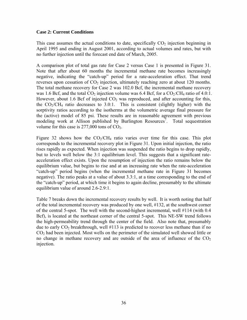
Case 2: Current Conditions This case assumes the actual conditions to date, specifically CO2 injection beginning in April 1995 and ending in August 2001, according to actual volumes and rates, but with no further injection until the forecast end date of March, 2005. A comparison plot of total gas rate for Case 2 versus Case 1 is presented in Figure 31. Note that after about 60 months the incremental methane rate becomes increasingly negative, indicating the “catch-up” period for a rate-acceleration effect. That trend reverses upon cessation of CO2 injection, ultimately reaching zero at about 120 months. The total methane recovery for Case 2 was 102.0 Bcf, the incremental methane recovery was 1.6 Bcf, and the total CO2 injection volume was 6.4 Bcf, for a CO2:CH4 ratio of 4.0:1. However, about 1.6 Bcf of injected CO2 was reproduced, and after accounting for this, the CO2/CH4 ratio decreases to 3.0:1. This is consistent (slightly higher) with the sorptivity ratios according to the isotherms at the volumetric average final pressure for the (active) model of 85 psi. These results are in reasonable agreement with previous modeling work at Allison published by Burlington Resources7. Total sequestration volume for this case is 277,000 tons of CO2. Figure 32 shows how the CO2/CH4 ratio varies over time for this case. This plot corresponds to the incremental recovery plot in Figure 31. Upon initial injection, the ratio rises rapidly as expected. When injection was suspended the ratio begins to drop rapidly, but to levels well below the 3:1 equilibrium level. This suggests that a significant rate-acceleration effect exists. Upon the resumption of injection the ratio remains below the equilibrium value, but begins to rise and at an increasing rate when the rate-acceleration “catch-up” period begins (when the incremental methane rate in Figure 31 becomes negative). The ratio peaks at a value of about 3.3:1, at a time corresponding to the end of the “catch-up” period, at which time it begins to again decline, presumably to the ultimate equilibrium value of around 2.6-2.9:1. Table 7 breaks down the incremental recovery results by well. It is worth noting that half of the total incremental recovery was produced by one well, #132, at the southwest corner of the central 5-spot. The well with the second-highest incremental, well #114 (with 0.4 Bcf), is located at the northeast corner of the central 5-spot. This NE-SW trend follows the high-permeability trend through the center of the field. Also note that, presumably due to early CO2 breakthrough, well #113 is predicted to recover less methane than if no CO2 had been injected. Most wells on the perimeter of the simulated well showed little or no change in methane recovery and are outside of the area of influence of the CO2 injection.

37

-100,000

-50,000

0

50,000

100,000

150,000

200,000

0 20 40 60 80 100 120

Month

Gas

Rat

e, M

cf/M

o

Total Gas Produced Total CH4 Produced Total CO2 Produced Injected Gas

Figure 31: Incremental Gas Rates, Case 2 versus Case 1

0

0.5

1

1.5

2

2.5

3

3.5

4

0 20 40 60 80 100 120 140 160 180 200

Months after Initial Injection

Net C

O2/

CH

4 Ra

tio

Injection Suspended

Injection Stopped

Injection Resumed

Rate Acceleration “Catch-up” Period

0

0.5

1

1.5

2

2.5

3

3.5

4

0 20 40 60 80 100 120 140 160 180 200

Months after Initial Injection

Net C

O2/

CH

4 Ra

tio

Injection Suspended

Injection Stopped

Injection Resumed

Rate Acceleration “Catch-up” Period

Figure 32: CO2/CH4 Ratio as a Function of Time

38

Table 7: Case 2 – Incremental Methane Recoveries by Well

Well Without Injection (Bcf) With Injection (Bcf)

Incremental (Bcf)

101

1.0

1.0

------

102 6.3 6.4 0.1 104 3.1 3.2 0.1 106 8.2 8.2 ----- 108 6.3 6.3 ----- 111 3.3 3.1 (0.2) 112 5.7 5.8 0.1 113 10.4 9.5 (0.9) 114 10.3 10.7 0.4 115 6.0 6.2 0.2 119 10.4 10.4 ----- 120 5.6 5.9 0.3 121 7.3 7.6 0.3 130 4.8 5.1 0.3 131 5.6 5.7 0.1 132 6.1 6.9 0.8

TOTAL 100.4 102.0 1.6

39

Case 3: Continuous Future CO2 Injection This case assumes that CO2 injection resumed in January, 2003, at a constant rate approximately equal to the last recorded rates (1,000 Mcf/day for wells #140, #141, #142 and 500 Mcf/day for well #143). The forecast end date was June, 2011 (8 ½ years after resumption of CO2 injection). A plot of incremental gas rate for Case 3 versus Case 2 is presented in Figure 33. Note that several wells were shut-in due to exceeding the maximum CO2 content criteria of the produced gas (50%). The total methane recovery for Case 3 was 103.6 Bcf and the incremental methane recovery over Case 2 was 1.6 Bcf. The total incremental CO2 injection volume was 11.1 Bcf, for a CO2:CH4 ratio of 6.9:1. After accounting for about 0.4 Bcf of incremental reproduced CO2, this ratio declines to 6.7:1. Volumetric average final pressure for the (active) model was 98 psi. Incremental sequestration volume for this case is 618,000 tons of CO2.


-10000

0

10000

20000

30000

40000

50000

0 20 40 60 80 100 120 140 160 180 200

Months after first injection (April '95)

Gas

Rat

e, M

cf/M

o

0

20000

40000

60000

80000

100000

120000

Inje

cted

Gas

Rat

e, M

cf/M

o


#120 shut-in

#113 shut-in

#132 shut-in

40

Case 4: Limited Future CO2 Injection Rather than continuous future CO2 injection, Case 4 assumes CO2 injection for a period of 12 months, also starting in January, 2003, and at the same rates as Case 3. The forecast end date was June, 2011. A plot of incremental gas rate for Case 4 versus Case 2 is presented in Figure 34. The total methane recovery for Case 4 was 102.4 Bcf and the incremental methane recovery over Case 2 was 0.4 Bcf. The total incremental CO2 injection volume was 1.3 Bcf, for a CO2:CH4 ratio of 3.3:1. After accounting for about 0.2 Bcf of incremental reproduced CO2, this ratio decreases to 2.7:1. Volumetric average final pressure for the (active) model was 85 psi. Incremental sequestration volume for this case is 64,000 tons of CO2.

0

2,000

4,000

6,000

8,000

10,000

12,000

14,000

0 50 100 150 200


Gas

Rat

e, M

cf/M

o

0

20,000

40,000

60,000

80,000

100,000

Inje

cted

Gas

Rat

e, M

cf/M

o

Total Produced Gas Total Produced CH4 Total Produced CO2 Injected CO2


41

Case 5: Aggressive, Continuous Future CO2 Injection It is clear from the preceding forecast cases that CO2 injection volumes are limited, and as such so too are the incremental methane recoveries. For improved economic performance, given the sunk capital costs involved, higher CO2 injection volumes would be beneficial. While it is acknowledged that to achieve higher injection rates, some work to the injection wells would be required to improve injectivity, this case is worth evaluating. To do so, Case 5 assumes injection rates at four times those of the preceding cases, or 4,000 Mcf/day for wells #140, #141, #142 and 2,000 Mcf/day for well #143. Consistent with the earlier cases, injection resumed in January 2003 and the forecast end date was June, 2011. A plot of incremental gas rate for Case 5 versus Case 2 is presented in Figure 35. Note that many wells were shut-in for exceeding the maximum CO2 content criteria for the produced gas of 50%. The total methane recovery for Case 5 was 106.3 Bcf, and the incremental methane recovery over Case 2 was 4.3 Bcf. The total incremental CO2 injection volume was 45.2 Bcf, for a CO2:CH4 ratio of 10.5:1. After accounting for 1.4 Bcf of incremental reproduced CO2, this ratio decreased to 10.2:1. Volumetric average final pressure for the (active) model was 154 psi. Incremental sequestration volume for this case is 2.5 million tons of CO2.

Figure 35: Total and Incremental Gas Rates, Case 5 versus Case 2

-20000

0

20000

40000

60000

80000

0 20 40 60 80 100 120 140 160 180 200


Gas

Rat

e, M

cf/M

o

0

100000

200000

300000

400000

500000

Inje

cted

Gas

Rat

e, M

cf/M

o


#112 #113 & 120 shut-in

#132

#114#131 #115

#130

42

Case 6: Aggressive, Limited Future CO2 Injection This case also assumes aggressive CO2 injection (at a rate four times the earlier rate), but for a period of only 12 months. Again, injection start date was January 2003 and the forecast end date was June, 2011. A plot of incremental gas rate for Case 6 versus Case 2 is presented in Figure 36. Note that several wells were shut-in for exceeding the maximum CO2 content criteria for the produced gas of 50%. The total methane recovery for Case 6 was 103.3 Bcf, and the incremental methane recovery over Case 2 was 1.3 Bcf. The total incremental CO2 injection volume was 5.4 Bcf, for a CO2:CH4 ratio of 4.1:1. After accounting for 0.5 Bcf of reproduced CO2, this ratio decreases to 3.8:1. The Volumetric average final pressure for the active model area was 87 psi. Incremental sequestration volume for this case is 283,000 tons of CO2.

-10000

0

10000

20000

30000

40000

50000

60000

0 20 40 60 80 100 120 140 160 180 200


Gas

Rat

e, M

cf/M

o

0

100000

200000

300000

400000

500000

Inje

cted

Gas

Rat

e, M

cf/M

o

Total Gas Produced Total CH4 Produced Total CO2 produced Injected Gas


#120 shut-in #113 shut-in

43

A summary of the results for each run is presented in Table 8.

Table 8: Summary of Model Forecast Results

Case 1 Case 2 Case 3 Case 4 Case 5 Case 6 Total CH4 Produced (Bcf) 100.4 102.0 103.6 102.4 106.3 103.3

Incremental CH4 (Bcf) 0 1.6 3.2 2.0 5.9 2.9 Incremental CH4 Recovery (% OGIP) 0 1.1% 2.1% 1.3% 3.9% 1.9%

Total CO2 Injected (Bcf) 0 6.4 17.5 7.7 51.6 11.8

Total CO2 Produced (Bcf) 7.7 9.3 9.7 9.5 10.7 9.8

CO2/CH4 Ratio 0 3.0 4.8 3.0 8.2 3.3 It is clear from these results that, while the absolute values of incremental methane recoveries seem reasonable in relation to the injected CO2 volumes, particularly in those cases where the reservoir system was allowed to equilibrate (i.e., CO2 injection ceased a production continued, allowing the CO2 to work its way through the reservoir, resulting in a CO2/CH4 ratio of about 3:1), the incremental recoveries in terms of percentage of original gas-in place (OGIP) are almost insignificant and warrant further examination. In the cases where the CO2/CH4 ratios exceed 3-3½:1, one should expect that had injection ceased and the forecast period been extended, incremental methane recovery would have increased (and some injected CO2 reproduced) to bring that ratio into line. The implication is that to achieve the “equilibrium” CO2/CH4 replacement ratio specific to a given reservoir setting (about 3:1 in this case), some time is required after the cessation of CO2 injection for the system to equilibrate.

44

9.0 Discussion of Results The most striking result from the forecasts is that so little incremental methane is recovered, particularly when stated as a percentage of OGIP. (It is worth reiterating that due to more rapid CO2 breakthrough in the model than actually observed, incremental methane recoveries are understated.) As a first step in understanding the forecast results, it is useful to examine the CO2/CH4 ratios. Figure 37 presents the equilibrium CO2/CH4 ratios based on the isotherms presented in Figures 10 and 11. Note that, for these specific isotherms, the ratio increases with decreasing pressure (and are fairly consistent for each seam). For the ending reservoir pressures for the cases presented in the previous section (typically 80 to 100 psi), the equilibrium ratio is approximately 2.6 – 2.9. Thus, in those cases with ratios of 3-3½:1 (where injection ceased and production continued), the ratio is approximately the equilibrium value, accounting for some system inefficiencies.

0.00

0.50

1.00

1.50

2.00

2.50

3.00

3.50

0 500 1000 1500 2000 2500 3000

Pressure, psi

CO

2/C

H4

Rat

io

Yellow

Blue

Purple

Figure 37: CO2/CH4 Sorption Ratios, Case 2

The primary problem at Allison was that, due to significant permeability and injectivity loss with CO2 injection, only limited volumes of CO2 could be injected. Finding ways to overcome or prevent this type of permeability/injectivity loss is therefore an important topic for future research, and critical if CO2-ECBM/sequestration is to become a viable sequestration option. Another aspect of the Allison results to keep in perspective is that the effects of CO2 injection were primarily observed in the central 5-spot pattern, and not the outer reaches of the model area, where a large portion of the 152 Bcf OGIP resides. If one takes an

45

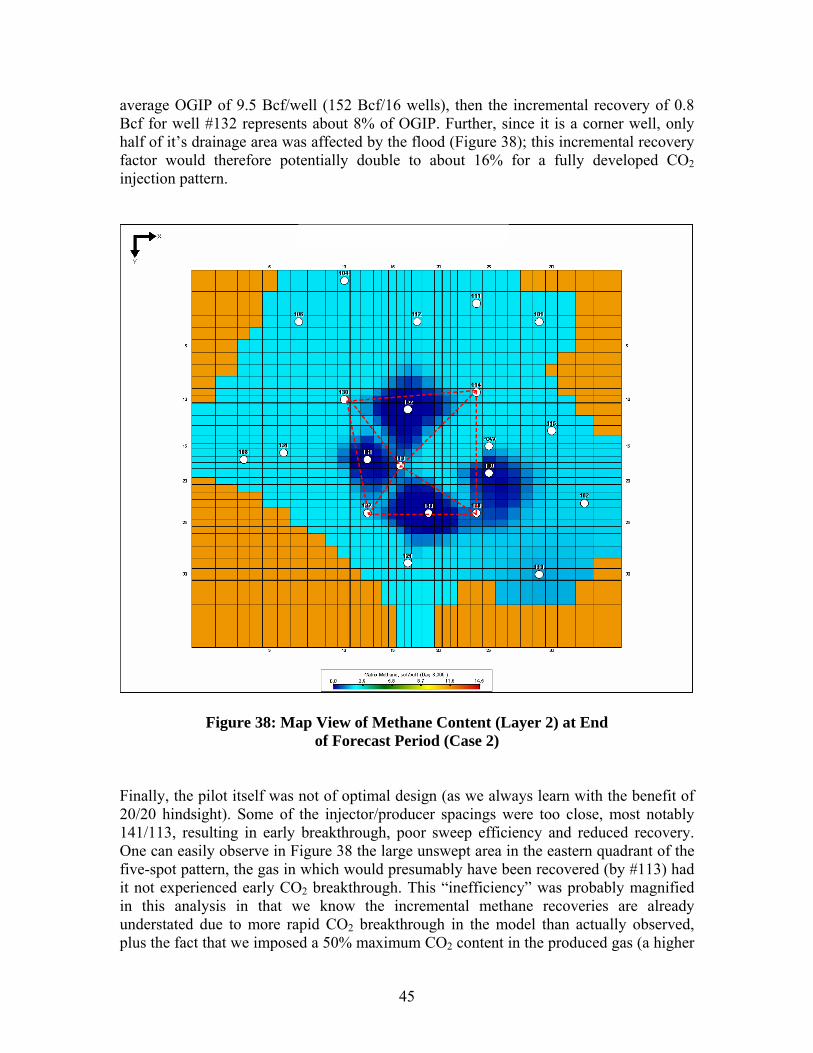
average OGIP of 9.5 Bcf/well (152 Bcf/16 wells), then the incremental recovery of 0.8 Bcf for well #132 represents about 8% of OGIP. Further, since it is a corner well, only half of it’s drainage area was affected by the flood (Figure 38); this incremental recovery factor would therefore potentially double to about 16% for a fully developed CO2 injection pattern.

Figure 38: Map View of Methane Content (Layer 2) at End of Forecast Period (Case 2)

Finally, the pilot itself was not of optimal design (as we always learn with the benefit of 20/20 hindsight). Some of the injector/producer spacings were too close, most notably 141/113, resulting in early breakthrough, poor sweep efficiency and reduced recovery. One can easily observe in Figure 38 the large unswept area in the eastern quadrant of the five-spot pattern, the gas in which would presumably have been recovered (by #113) had it not experienced early CO2 breakthrough. This “inefficiency” was probably magnified in this analysis in that we know the incremental methane recoveries are already understated due to more rapid CO2 breakthrough in the model than actually observed, plus the fact that we imposed a 50% maximum CO2 content in the produced gas (a higher

46

number, if operationally feasible, would also have the effect of increasing methane recovery). In summary, the results from Allison do make sense, and the low incremental methane recoveries on a gross basis are understandable. However, the requirements for higher recoveries are also clear – specifically larger injection volumes, enhanced injectivity, and optimal well placement.

47

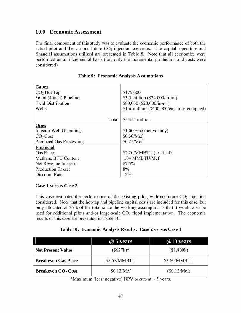
10.0 Economic Assessment The final component of this study was to evaluate the economic performance of both the actual pilot and the various future CO2 injection scenarios. The capital, operating and financial assumptions utilized are presented in Table 8. Note that all economics were performed on an incremental basis (i.e., only the incremental production and costs were considered).

Table 9: Economic Analysis Assumptions

Capex CO2 Hot Tap: 36 mi (4 inch) Pipeline: Field Distribution: Wells

Total

$175,000 $3.5 million ($24,000/in-mi) $80,000 ($20,000/in-mi) $1.6 million ($400,000/ea; fully equipped) $5.355 million

Opex Injector Well Operating: CO2 Cost Produced Gas Processing

$1,000/mo (active only) $0.30/Mcf $0.25/Mcf

Financial Gas Price: Methane BTU Content Net Revenue Interest: Production Taxes: Discount Rate:

$2.20/MMBTU (ex-field) 1.04 MMBTU/Mcf 87.5% 8% 12%

Case 1 versus Case 2 This case evaluates the performance of the existing pilot, with no future CO2 injection considered. Note that the hot-tap and pipeline capital costs are included for this case, but only allocated at 25% of the total since the working assumption is that it would also be used for additional pilots and/or large-scale CO2 flood implementation. The economic results of this case are presented in Table 10.

Table 10: Economic Analysis Results: Case 2 versus Case 1

@ 5 years @10 years Net Present Value ($627k)* ($1,809k)

Breakeven Gas Price $2.57/MMBTU $3.60/MMBTU

Breakeven CO2 Cost $0.12/Mcf ($0.12/Mcf)

*Maximum (least negative) NPV occurs at ~ 5 years.

48

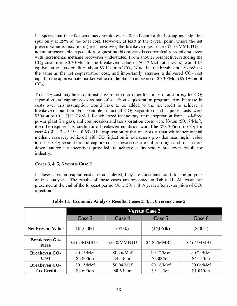
It appears that the pilot was uneconomic, even after allocating the hot-tap and pipeline spur only at 25% of the total cost. However, at least at the 5-year point, where the net present value is maximum (least negative), the breakeven gas price ($2.57/MMBTU) is not an unreasonable expectation, suggesting this process is economically promising, even with incremental methane recoveries understated. From another perspective, reducing the CO2 cost from $0.30/Mcf to the breakeven value of $0.12/Mcf (at 5-years) would be equivalent to a tax credit of about $3.11/ton of CO2. Note that the breakeven tax credit is the same as the net sequestration cost, and importantly assumes a delivered CO2 cost equal to the approximate market value (in the San Juan basin) of $0.30/Mcf ($5.19/ton of CO2). This CO2 cost may be an optimistic assumption for other locations, or as a proxy for CO2 separation and capture costs as part of a carbon sequestration program. Any increase in costs over this assumption would have to be added to the tax credit to achieve a breakeven condition. For example, if actual CO2 separation and capture costs were $30/ton of CO2 ($11.73/Mcf, for advanced technology amine separation from coal-fired power plant fire gas), and compression and transportation costs were $3/ton ($0.17/Mcf), then the required tax credit for a breakeven condition would be $28.50/ton of CO2 for case 4 (30 + 3 – 5.19 + 0.69). The implication of this analysis is than while incremental methane recovery achieved with CO2 injection in coalseams provides meaningful value to offset CO2 separation and capture costs, these costs are still too high and must come down, and/or tax incentives provided, to achieve a financially breakeven result for industry. Cases 3, 4, 5, 6 versus Case 2 In these cases, no capital costs are considered; they are considered sunk for the purpose of this analysis. The results of these cases are presented in Table 11. All cases are presented at the end of the forecast period (June 2011, 8 ½ years after resumption of CO2 injection).

Table 11: Economic Analysis Results, Cases 3, 4, 5, 6 versus Case 2

Versus Case 2 Case 3 Case 4 Case 5 Case 6

Net Present Value ($1,040k) ($38k) ($5,063k) ($301k)

Breakeven Gas Price $3.67/MMBTU $2.38/MMBTU $4.82/MMBTU $2.64/MMBTU

Breakeven CO2 Cost

$0.15/Mcf $2.60/ton

$0.26/Mcf $4.50/ton

$0.12/Mcf $2.08/ton

$0.24/Mcf $4.15/ton

Breakeven CO2 Tax Credit

$0.15/Mcf $2.60/ton

$0.04/Mcf $0.69/ton

$0.18/Mcf $3.11/ton

$0.06/Mcf $1.04/ton

49

Similar to the previous case, each of these cases appear to favor short-term CO2 injection (cases 4 and 6) over long-term injection (cases 3 and 5) from an ECBM economic perspective. However, purely from a CO2 sequestration perspective, tax credits of generally <$3/ton of CO2 would be required for a profitable sequestration operation, again considering the reasonableness of the CO2 cost assumptions

50

11.0 Case for Carbon Sequestration Since all previous runs were considered primarily from an ECBM economic optimization perspective, and since this study was funded under DOE’s carbon sequestration program, a final simulation was performed to evaluate the economic results for maximum CO2 sequestration. For this run case 5 was merely extended until all wells were shut-in, and the reservoir pressure reached 75% of the original pressure, or 1,240 psi. This assumes that the original CO2 injection was performed on a stand-alone ECBM basis (to cover the capital costs for injection), and that the field was then converted to sequestration service. The results of this case, which ran to January 2038 (35 years after resumption of injection in January 2003), suggested a total methane recovery of 111.4 Bcf, and an incremental methane recovery of 9.4 Bcf. The total incremental CO2 injection volume was 178.6 Bcf. After accounting for 3.5 Bcf of incremental reproduced CO2, the total incremental sequestration volume is over 10 million tons of CO2, or 2.8 million tons of carbon. The large volume of unrecovered methane (over 40 Bcf) is probably due to the fact that the wells were shut-in when CO2 content reached 50%, and that the model predicts CO2 breakthrough too early (i.e., incremental methane recovery is understated). The pressure history for the model area is shown in Figure 39.

Field on Production

Begin Initial CO2Injection Pilot

End of Actual History

Begin Aggressive CO2 Injection

Proposed Stop of

Injection (Pr = 0.75 Pi)

Methane Depletion and ECBM Period

CO2 Sequestration Period

End of Forecast Period

Field on Production

Begin Initial CO2Injection Pilot

End of Actual History

Begin Aggressive CO2 Injection

Proposed Stop of

Injection (Pr = 0.75 Pi)

Methane Depletion and ECBM Period

CO2 Sequestration Period

End of Forecast Period

Figure 39: Reservoir Pressure History for the CO2 Sequestration Cost

51

Economic assessment on this basis yields a breakeven CO2 cost of $0.12/Mcf, which equates to a breakeven tax credit of $3.11/ton of CO2 or $11.41/ton of carbon. These results suggest that large CO2 volumes can potentially be sequestered at reasonable net costs in coalseams.

52

12.0 Conclusions Based on the results of this study, the following conclusions have been drawn:

o The injection of CO2 at the Allison Unit has resulted in incremental methane recovery over estimated ultimate primary recovery, in approximately a proportion of one volume of methane for every three volumes of CO2 injected.

o The study area was successfully modeled with ARI’s COMET2 model. However,

aspects of the model remain uncertain, such as producing and injecting bottomhole pressures, CO2 content profiles of the produced gas, and the pressure at the observation well.

o There appears to be clear evidence of significant coal permeability reduction with

CO2 injection. This permeability reduction, and the associated impact on CO2 injectivity, compromised incremental methane recoveries and project economics. Finding ways to overcome and/or prevent this effect is therefore an important topic for future research.

o From a CO2 sequestration standpoint, the incremental methane recoveries (based

solely on the conditions encountered at the Allison Unit), can provide a meaningful offset to CO2 separation, capture and transportation costs, on the order of $2–5/ton of CO2.

53

13.0 Nomenclature ARI - Advanced Resources International Bcf - billions of cubic feet BTV - British Thermal Units C - absorbed gas concentration Capex - capital expenditures CBM - coalbed methane cc - cubic centimeters CH4 - methane Ci - initial adsorbed gas concentration Ck - differential swelling factor cm - matrix compressibility CO2 - carbon dioxide Cp - pore volume compressibility Ct - total absorbed gas concentration DOE - Department of Energy $ - dollars (U.S.) E - Young’s modulus, psi ECBM - enhanced coalbed methane recovery f - decimal fraction, dimensionless FOI - folds of increase ft - feet g - grams Gt - gigatonnes k - permeability, millidarcy kabs - absolute permeability keg - effective gas permeability ki - initial permeability, millidarcy M - constrained axial modulus, psi Mcf - thousand of cubit feet Mcfd - thousands of cubic feet per day md - millidarcies mo - month

54

MUGS - Model of Unconventional Gas Supply MW - megawatts n - permeability exponent N2 - nitrogen NPV - net present value ºF - degrees Fahrenheit OGIP - original gas in place Opex - operating expenditures P - pressure % - percent Pi - initial pore pressure PL - Langmuir pressure psi - pounds per square inch psia - pounds per square inch absolute PTA - pressure transient analysis SCF - standard cubic feet Sm - matrix swelling coefficient, ton/scf SMV - storage monitoring and verification Tcf - trillions of cubic feet Tmv - time value of money U.S. - United States VL - Langmuir volume vs - versus β - inverse of Langmuir pressure, psi-1 γ - grain compressibility, psi-1 εL - Langmuir strain, dimensionless εm - bulk strain due to matrix swelling, dimensionless υ - Poisson’s ratio Φ - porosity Φi - initial porosity

55

14.0 Acknowledgements The authors also wish to acknowledge the valuable contribution of Burlington Resources, which provided all the data for the study, invaluable insights, and permission for the results to be published.

56

15.0 References 1. Reeves, S. R.: “Geologic Sequestration of CO2 in Deep, Unmineable Coalbeds: An Integrated Research and Commercial-Scale Field Demonstration Project”, SPE 71749, presented at the SPE Annual Technical Conference and Exhibition, New Orleans, September 30-October 3, 2001. 2. Reeves, S. and Pekot, L.: “Advanced Reservoir Modeling in Desorption-Controlled Reservoirs,” SPE 71090, presented at the SPE Rocky Mountain Petroleum Technology Conference, Keystone, May 21-23, 2001. 3. Paul, G.W. and Young, G.B.C.: “Characterization of Fruitland Coal through Reservoir Simulation,” GRI Topical Report GRI-92/0461, November, 1993. 4. Pekot, L. and Reeves, S.: “Modeling Coal Matrix Shrinkage and Differential Swelling with CO2 Injection for Enhanced Coalbed Methane and Carbon Sequestration Applications,” DOE Topical Report prepared by Advanced Resources International, November, 2002, in review. 5. Sawyer, W.K., Paul, G.W., Schraufnagel, R.A., “Development and Application of a 3D Coalbed Simulator,” CIM/SPE 90-119, presented at the CIM/SPE International Technical Conference, Calgary, June 10-13, 1990. 6. Gasem, K.A.M., Robinson, R.L., and Reeves, S.R.: “Adsorption of Pure Methane, Nitrogen, and Carbon Dioxide and Their Mixtures on San Juan Basin Coal”, DOE Topical Report prepared by Oklahoma State University, May, 2002. 7. Schoeling, L. and McGovern, M.: “Pilot Test Demonstrates How CO2 Injection Enhances Coalbed Methane Recovery,” Petroleum Technology Digest, supplement to World Oil magazine, September, 2000.

A-1

Appendix A:

Comparison Plots - Initialization Run versus Actual Data Note: Actual data represented by square data points, simulated data by circle data points.

Date post:	12-Feb-2017
Category:	Documents
Upload:	ledung
View:	222 times
Download:	0 times

The Allison Unit CO2 – ECBM Pilot: A Reservoir Modeling Study

Documents