Economic Research Southern Africa (ERSA) is a research programme funded by the National

Treasury of South Africa. The views expressed are those of the author(s) and do not necessarily represent those of the funder, ERSA or the author’s affiliated

institution(s). ERSA shall not be liable to any person for inaccurate information or opinions contained herein.

The analysis of borders effects in intra-

African trade

Emilie Kinfack Djoumessi and Alain Pholo Bala

ERSA working paper 701

August 2017

The analysis of borders effects in intra-African trade

Emilie Kinfack Djoumessi∗ Alain Pholo Bala ∗†

August 23, 2017

Abstract

The study aims to analyze the border effects on intra–African trade through the use of a gravity

specification based on the monopolistic competition model of trade introduced by Krugman (1980).

The study used CEPII data on trade flows between African countries over the period 1980-2006.

We accommodate for the significant number of zero trade flows between several African countries

by using the Heckman correction method. The findings suggest that while the extent of market

fragmentation is on average very high within the African continent, the border effects within SADC

and ECOWAS are more in line with other international estimations. Whereas results indicate that

border effects faced by intra-African trade are quite substantial: on average an African country trade

108 times more “with itself” than with another country on the continent. Border effects in SADC

and ECOWAS are respectively about 5 and 3 times lower. The inclusion of the infrastructure indices

contributes significantly to this result. Considering infrastructure is actually an interesting way to

capture the effect of distribution networks which represent, along with imperfect information and

localized tastes, relevant but generally omitted sources of resistance.

Keyword: Intra-African Trade, Monopolistic Competition Model, Border Effect

JEL Classification: F12, F14, F15

1 Introduction

The analysis of economic growth in sub-Saharan Africa (SSA) has raised some major concerns in the De-

velopment Economics literature (Collier, 2006a,b; Dollar and Easterly, 1999; Easterly and Levine, 1997;

Easterly, 2009a,b). While this continent has experienced strong economic growth rates lately (Pinkovskiy

and Sala-i Martin, 2014), until the 1990s SSA was characterized by low and even sometimes negative

∗Department of Economics & Econometrics, University of Johannesburg, APK Campus, PO Box 524, Auckland Park

2006, Johannesburg, South Africa.†Public and Environmental Economics Research Centre (PEERC), Corresponding author. E-mail address:

apholo@uj.ac.za.

1

economic growth (Cinyabuguma and Putterman, 2011; Easterly and Levine, 1997; Sachs and Warner,

1997; Artadi and Sala-i Martin, 2003).

Several impediments specific to the African growth process have been identified. Among them, we

may consider that SSA is badly affected by low population density, long distances and high fragmenta-

tion (World Bank, 2008). High transport costs add to the high fragmentation of that region. For goods

to pass the border in Africa, it takes more than 40 days which is twice the period in Latin America.

The constraints are even worse for landlocked countries (Freire et al., 2015).

Collier (2006a) asserts that agglomeration economies in SSA are less important than those prevailing

in Asia and in OECD countries. Because countries in that region are too small and not integrated

enough, many African cities tend to be too small compared to the optimum. As shown by Au and

Henderson (2006) in the case of Asia, this may have serious impacts in terms of foregone growth.

Research on agglomeration economies and international competitiveness further suggests that late-

comers to industrialization, such as Africa’s natural resource exporters, face a competitive disadvantage

linked to the spatial distribution of the global industry (Page, 2008).

Africa appears as fragmented and poorly integrated. Intra-regional trade in the region is fairly low

comparatively to what is noticed in other areas. Therefore, improving regional integration appears as

one of the key strategies that might foster economic growth in the African continent. Better regional

integration might help SSA achieve greater economies of scale, widen markets, enhance industrial effi-

ciency, and reduce the sub-region’s external dependency and vulnerability of its economy (Jones, 2002).

The other benefits that may be expected from an increased regional integration are the following: a

greater bargaining power vis-a-vis the outside world; the minimization of duplication; thin spreading of

resources and wasteful competition; a cheaper and more efficient transportation system; greater divi-

sion of labor and specialization in production; established and strengthened product value chains and

facilitated transfer of technology and knowledge via spillover effects; expansion of trade, incomes and

employment due to free movement of goods, services, labor and capital, etc. (Jones, 2002; UNECA,

2010).

Another argument exists for promoting intra-African trade. To take advantage of trade-growth

opportunities, SSA is prompted to diversify in several ways: one way would be by reducing its reliance

on the stagnating markets of its traditional trading partners from the Organisation for Economic Co-

operation and Development (OECD). Concurrently, it needs to become less dependent on the export of

commodities vulnerable to price shocks (ITC, 2012). The redirection of SSA exports towards Asia, and

China in particular, is already underway. However, since the large majority of SSA products destined

for Asia are commodities, such a reorientation to growth markets does not eradicate the vulnerability to

commodity price shocks. SSA countries increasingly trade within their own region too. This new trend

of SSA trade is likely to achieve sustainability in export revenues by integrating deeper into sector value-

chains and in this way increasing the share of value-added products within its exports. The redirection

of SSA exports towards Africa may further reduce the risks caused by the volatility of commodity price

2

shocks.

However, despite Africa’s commitment to ease trade restrictions in order to create a common market

within the framework of Regional Economic Communities (RECs) and the reorientation of its trade,

barriers to intra-African trade tend to persist. On average over the past decade, only about 10%-12%

of African trade has been with African nations, while 40% of North American trade has been with

other North American countries, and 63% of trade in Western Europe is with other Western European

nations (Economic Commission for Africa, 2011). Intra-African trade is also low when compared to

that of other developing regions; intra Latin America trade amounts to 20 % while trade within Asian

developing countries represents 48 % (Ancharaz et al., 2011). In this regard, SSA’s trade seems to be

extroverted as a substantial share of it is directed to the developed world: in 2011 more than half of

SSA’s merchandise trade was still done with the OECD partners (ITC, 2012).

The orientation of most of African trade towards developed partners raises the issue of the effec-

tiveness of trade integration policies throughout African countries and RECs. In this paper, we assess

the effectiveness of the strategies adopted by African countries and regional groupings to foster trade

integration. We do so by evaluating the extent of border effects in intra-African trade. The intensity of

border effects helps to characterize the extent of market fragmentation. The term “border effect” refers

to the downward impact of national boundaries on the volume of trade, i.e. that two different countries

trade far less with each other than do two locations in the same country, after controlling for factors such

as income, alternative trading opportunities, distance, languages, and regional trade agreements (Evans,

2003). Markets are considered fragmented when national borders influence the pattern of commercial

transactions (Head and Mayer, 2000).

Using border effects to measure the extent of market fragmentation is more robust than using market

shares. As pointed out by de Sousa et al. (2012), while they are insightful, the market shares referred

to above cannot be sufficient to draw conclusions on the level of market fragmentation faced by African

exporters on the intra-regional market. The first problem is that any assessment of market access based

on trade flows needs to specify a benchmark of trade patterns, to which actual international exchanges

of goods will be compared. Without such a benchmark, which can only be provided by theory, we do

not know what to compare those numbers to. This need of a reference for comparison justifies why we

will derive an empirically estimable gravity-type equation from a theoretical framework.

A second limitation implied by the use of the import shares to assess market access is that for most

products, the large majority of overall demand in a country is met by domestic producers, not foreign.

A more relevant index of market access must take into account the market share of foreign producers

in the overall demand. This is precisely what the border effects method does. The method considers

trade flows within countries as well as among countries and compares imports from foreign countries to

“imports from self” of domestic producers. Hence, this approach gives a benchmark based on a situation

of the best possible market access, the one faced by domestic producers (de Sousa et al., 2012).

Border effects matter when firms have greater access to domestic consumers than to consumers in

3

other nations. Following Head and Mayer (2000), we measure border effects as the average spread be-

tween actual trade and the trade that would be expected in an economy without border-related barriers.

To capture border effects we rely on a gravity model. The gravity model offers a powerful empirical

framework for analyzing bilateral trade flows (Anderson and van Wincoop, 2003; Behrens et al., 2012).

However, the specification of gravity models has improved significantly over time. With an ad hoc spec-

ification linking bilateral trade flows to importer and exporter GDP and bilateral distance, McCallum

(1995) found an impressive border effect between the Canadian provinces and the United States, i.e.

the trade between two provinces is more than 20 times larger than trade between a province and an

American state. These findings, which were confirmed by Helliwell (1996) and Hillberry (1998), suggest

a very large degree of home bias in trade within North-America . One of the implication of the so-called

“border puzzle” would be that international trade flows would remain much less dense than national

trading ties even after all tariffs were removed.

However, some serious concerns have been raised on this first wave of studies. Anderson and van

Wincoop (2003) pointed out that the lack of theoretical foundation of gravity equations has two adverse

consequences. First, estimation results are likely to be biased because of omitted variables. Second, it

is not possible to conduct a comparative statics exercise. Therefore, Anderson and van Wincoop (2003)

used an estimated general equilibrium model to solve the “border puzzle”. Anderson and van Wincoop

(2003)’s model modifies McCallum (1995)’s specification by adding “multilateral resistance” variables.

Applying their model to 1993 data, Anderson and van Wincoop (2003) found only moderate impact of

trade barriers on trade flows: borders reduce trade between USA and Canada by 44%, and trade among

other industrialized countries by 29%.

In this paper, we follow Head and Mayer (2000) and Combes et al. (2005) by performing a structural

estimation based on the monopolistic competition model of trade proposed by Krugman (1980). That

Krugman model derives a relation between the relative amounts consumers spend on foreign and domes-

tic goods and their relative prices. The border effect is captured by the divergence between actual and

predicted consumption ratios. The remainder of the paper is organized as follows. Section 2 presents

the theoretical model and the implied econometric specifications. The data are described in Section 3.

And finally, the econometric results are given in Section 4.

2 Model

Several theory-consistent estimation methods for the gravity model exist (Head and Mayer, 2013a). With

the data at hand, bilateral trade flow between countries per industry, we can estimate border effects

only through the complete odds specification as in Head and Mayer (2000) and Combes et al. (2005).1

Therefore, we follow Head and Mayer (2000)’s and Combes et al. (2005)’s approach of including border

effects into a monopolistic competition model. We use a fairly broad specification of preferences. The

utility of the representative consumer in country i depends on the quantity of each variety h consumed

4

from each country j. We assume that all varieties are differentiated from each other but products from

the same country are weighted equally in the utility function. Representing the quantity consumed with

c and the preference weight with a, the constant elasticity of substitution utility function is given by:

Ui =

N∑j=1

nj∑h=1

(aijcijh)σ−1σ

σσ−1

, (1)

while the implied budget constraint is

Yi =N∑j=1

nj∑h=1

pijhcijh (2)

We may simplify the consumer optimization problem by assuming that all quantities of the varieties

imported by country i from country j are symmetric. Then, denoting mij as the CIF value of exports

from country j to country i (mij = njcijpij) and mi =

N∑k=1

mik as expenses on goods from all origins

(including the home country), one may obtain the following expression of bilateral imports after some

algebra

mij =njp

1−σij aσ−1

ij

N∑k=1

nkp1−σik aσ−1

ik

mi. (3)

2.1 Econometric specifications

A gravity equation may be derived from this expression and may lead to different econometric specifi-

cations. As the number of symmetric varieties is not observed, we may eliminate nj and nk in equation

(3) by substituting them from equation (4)

νj = qpjnj (4)

where νj denotes the value of production in country j, q represents the quantity produced by each firm

and pj denotes the mill price of each variety. Considering the determination of delivered prices, pij , and

of preferences, aij , we assume that the price paid by consumers in country i for products of country j

is the product of the mill price, pj , and of transaction costs Tij

pij = pjTij (5)

We model transaction costs as a multiplicative function of the distance dij ; of the bilateral industry

level tariffs τij ; of the Non Tariffs Barriers (NTBs); of the level of infrastructure of the country i (j)

(INi(j)), and of an exponential function involving a contiguity dummy Cij . Furthermore, we assume

constant ad valorem NTBs of ξ for all cross-border trade. Defining Bij as a dummy variable taking a

5

value of one for i 6= j, we obtain

Tij = dδ1ij tδ2ij

[(1 + ξ) INi

−δ3INj−δ4e−δ5Cij

]Bij, (6)

with the tariff factor tij expressed as tij = 1 + τij .

Consumer preferences consist of a stochastic component, εij , and a systematic preference for home-

produced goods (or aversion to foreign-made goods) of α. Moreover, we hypothesize that several vari-

ables may mitigate or accentuate home bias and therefore posit the following equation for preferences:

aij = exp[εij −

(α− β1Lij − β2Eij − β3COLij + β4Vij −R′ijφ

)Bij]

(7)

where Lij takes the value of one for pairs of countries that share a common official language, and zero

otherwise; Eij takes the value of 1 when a language is spoken by at least 9% of the population in both

countries i and j (ethnic language); COLij = 1 if countries i and j had a common colonizer; and Vij is

the volatility of the bilateral exchange rate between countries i and j. Rij depicts a vector composed

of indicator variables taking the value of one when both countries i and j belong to the same regional

groupings like SADC, ECOWAS, and COMESA or if countries i and j had a common colonizer after

1945; while φ is the corresponding vector of parameters. Substituting for aij , pij and nj in (3) and

taking logs we obtain the formulation of the gravity equation:

lnmij = lnmi + ln νj − (σ − 1) δ1 ln dij − (σ − 1) δ2 ln tij − σ ln pj − Ii (8)

− (σ − 1)[α− β1Lij − β2Eij − β3COLij + β4Vij −R′ijφ+ ln (1 + ξ)− δ3 ln INi − δ4 ln INj

− δ5Cij ]Bij + (σ − 1) εij

where Ii depicts the Head and Mayer (2000) importer’s “inclusive value” defined as follows:

Ii = ln

{N∑k=1

exp [ln νk − σ ln pk + (σ − 1) (−δ1 ln dik − δ2 ln tik + εik

−[α− β1Lik − β2Eik − β3COLik + β4Vik −R′ikφ+ ln (1 + ξ) + δ3 ln INi + δ4 ln INk − δ5Cik

]Bik)]}

The inclusive value captures the impact of the full range of potential suppliers to a given importer

by taking into account their size, distance and relative border effects. There are several problems in

estimating the influence of Ii (Head and Mayer, 2000). The most critical is that such an estimation

would rely on parameters that are already in the equation to be estimated. There are two ways of

sidestepping those problems. First, we may derive from equation (8) a fixed-effects specification fully

consistent with theory. An alternative specification is to define a complete odds specification by setting

j = i in (8) to obtain an expression for ln (mii), then to subtract ln (mii) from ln (mij).

As in Combes et al. (2005) and in the spirit of Hummels (1999) and Redding and Venables (2004),

6

it is possible to derive from equation (8) a fixed-effects specification fully consistent with our theoretical

model. This derivation implies replacing all destination-specific and origin-specific variables by two

groups of destination and origin fixed effects. Only variables varying both with origin and destination

are left in the regression.

However, this approach has several problems. First, it does not permit the estimation of all structural

parameters. In particular, σ the elasticity of substitution between varieties cannot be recovered. Second,

as the approach implies dropping internal trade flows, it approach excludes the possibility of estimating

border effects. Therefore, to be able to estimate structural parameters and to evaluate border effects

we rely on the complete odds specification.

2.2 The complete odds specification

Setting j = i in (8) to obtain an expression for ln (mii) and then, subtracting ln (mii) from ln (mij), we

obtain the following complete odds specification (Combes et al., 2005):

ln

(mij

mii

)= − (σ − 1) [α+ ln (1 + ξ)] + ln

(νjνi

)− σ ln

(pjpi

)− (σ − 1) δ1 ln

(dijdii

)− (σ − 1) δ2 ln tij + (σ − 1) δ3 ln INi + (σ − 1) δ4 ln INj + (σ − 1) δ5Cij (9)

+ (σ − 1)β1Lij + (σ − 1)β2Eij + (σ − 1)β3COLij − (σ − 1)β4Vij + (σ − 1)R′ijφ+ εij

where εij = (σ − 1) (εij − εii). This expression of the error term implies that errors are not independently

distributed. We account for this correlation in the estimation through a robust procedure, allowing

residuals of the same importing region to be correlated.

In other words, according to (9) the log of odds ratios is expected to increase with the log of relative

production ln(νjνi

), with the fact that both importer and exporter share common languages and had a

common colonizer after 1945 and to decrease with the logs of relative distance, ln(dijdii

), tariffs factor,

ln (1 + τij), bilateral exchange rate volatility Vij and relative price, ln(pjpi

).

The intercept in (9) may be described as the border effect. It is the average deviation between actual

trade and the trade that would be expected in an economy without border-related barriers. It clearly

captures the impact of NTBs (ξ) and home bias (α) as in Head and Mayer (2000).

Equation (9) implies a unit elasticity on relative production; thus it may be rewritten as

ln

(mij

mii

)− ln

(νjνi

)= − (σ − 1) [α+ ln (1 + ξ)]− σ ln

(pjpi

)− (σ − 1) δ1 ln

(dijdii

)− (σ − 1) δ2 ln tij + (σ − 1) δ3 ln INi + (σ − 1) δ4 ln INj + (σ − 1) δ5Cij (10)

+ (σ − 1)β1Lij + (σ − 1)β2Eij + (σ − 1)β3COLij − (σ − 1)β4Vij + (σ − 1)R′ijφ+ εij

Imposing a unit elasticity on relative production helps addressing two different econometric issues:

7

first, output and trade are jointly determined in equilibrium (Harrigan, 1996; Head and Mayer, 2000);

which entails an endogeneity problem. Moving relative production in the left-hand side as in (10) is a

way to handle this simultaneity issue without resorting to instrumental variables. This strategy may

address another problem: measurement error for production. As production information may be inexact

especially for developing countries of SSA, we may obtain biased coefficients estimates.

2.3 Heckman correction for sample selection bias

The monopolistic competition trade model assumes positive trade between each country pair in each

industry (Head and Mayer, 2000). More generally, most of the structural gravity models do not naturally

generate zero flows (Head and Mayer, 2013a). However, most trade data sets exhibit substantial fractions

of zeros (Head and Mayer, 2013a). Helpman et al. (2008) show that, at the country level, country pairs

that do not trade with each other or trade in only one direction account for about half the observations.

There are two implications of a prevalence of zeros (Head and Mayer, 2013a). First, trade models need

to be adjusted in order to accommodate zeros. Second, estimation methods should be revised to allow

for consistent estimates in the presence of a dependent variable having a high incidence of zeros.

Several approaches can be used to accommodate structural gravity models to a prevalence of ze-

ros (Head and Mayer, 2013a). One simple approach is to consider that zeros arise from a data recording

issue, that is “there are no “structural zeros” but only “statistical zeros”” (Head and Mayer, 2013a,

p. 50-51). Some structural models generate zeros endogenously by adding a fixed cost of exporting from

i to j (Helpman et al., 2008; Eaton et al., 2012).2 These models have the common characteristic that

zeros are more likely between small and/or distant countries (Baldwin and Harrigan, 2011; Head and

Mayer, 2013a). As log of zero is not defined, observations without positive bilateral trade are lost, which

results in systematic selection bias as shown in Head and Mayer (2013a).

To find out which estimators may be consistent when zeros are an endogenous component of the data-

generating process, Head and Mayer (2013a) compare several estimators with a Monte Carlo Simulation:

the Least Squares Dummy Variables (LSDV), the Eaton and Tamura (1994) (ET) Tobit model, the Eaton

and Kortum (2001) (EK) Tobit model, the Multinomial Pseudo-Maximum-Likelihood (Multinomial

PML), the Poisson PML and the Gamma PML. The main findings of this Monte Carlo simulation

exercise is that the choice of the most suitable estimator depends on the process generating the error

term. Under the Constant Variance to Mean Ratio (CVMR) assumption, Poisson or Multinomial PML

provide the best estimators. However, under the log-normality assumption the EK Tobit method should

be preferred.

The Heckman selection model was left out of the Monte Carlo simulation exercise. The reason

advanced by Head and Mayer (2013a) is that the method used by Helpman et al. (2008), the leading

paper using a Heckman based approach of zeros, is designed to uncover a different set of parameters

than the other approaches which estimate coefficients that combine extensive and intensive margins.

The critical challenge implied by the Heckman-based methods is the difficulty of finding an exclusion

8

restriction. One would preferably use a variable in the probit selection equation which according to the

theory can be excluded from the gravity regression equation. Since both equations have exporter and

importer invariant variables, this variable should be dyadic in nature (Head and Mayer, 2013a).

Given, the poor results obtained with the EK Tobit and the Poisson PML, in this paper we fol-

low Head and Mayer (2000) who used a two-step Heckman selection model for a complete odds specifi-

cation.3 For the exclusion restriction we follow Helpman et al. (2008) by using two indicators for high

entry barriers in both countries i and j. These entry costs are captured through their effects on the

number of days, the number of legal procedures, and the relative cost (as a percentage of GDP per

capita) for an entrepreneur to legally start operating a business.

More precisely this indicator takes the value of one for country pairs in which both the importing and

exporting countries have entry regulation measures above the cross-country median. The first indicator

uses the sum of the number of days and procedures above the median (for both countries) whereas

the other indicator uses the sum of the relative costs above the median (again for both countries). By

construction, these variables capture regulation costs that should not depend on the exports volume of

a particular country and therefore, should comply with the necessary exclusion restrictions.

Our Heckman selection model implies either (9) or (10) as the regression equation. Moreover, we

assume that the dependent variable is observed if the following selection equation is verified:

X ′ijϕ+ µ1INi + µ2INj + ηij > 0 (11)

where

ηij ∼ N (0, 1)

corr(εij , ηij) = ρ

and Xij represents a vector including all the bilateral regressors of either (9) or (10) in addition to the

high entry barriers indicators. ρ is the correlation between unobserved determinants of propensity to

export ηij and unobserved determinants of the log of odds ratios εij . Therefore, testing whether ρ = 0

is equivalent to testing if there is sample selection. Defining the indicator variable INDij to be equal

to 1 when country j exports to i and to 0 when it does not, the probability that j exports to i can be

formally expressed by the following probit equation:

Pr (INDij = 1|observed variables) = Φ(X ′ijϕ+ µ1INi + µ2INj

)(12)

where Φ (.) is the cumulative distribution function of the unit-normal distribution. The choice of the

regressors in the probit equation is consistent with the fact that variables that are commonly used in

gravity equations also affect the probability that two countries trade with each other (Helpman et al.,

2008).

9

3 Data requirements

In this paper we use trade and production data from the CEPII’s TradeProd database.4 This database

proposes bilateral trade, production and protection figures in a compatible industry classification for

developed and developing countries. It covers 28 industrial sectors in the ISIC Revision 2 (International

Standard Industrial Classification) from 1980 to 2006. We restrict our analysis to the trade flows between

African countries.

The relative prices are captured by the price level of consumption from the Penn World Tables

v.7.1. Bilateral information on the prevalence of common languages,5 contiguity and distances are

obtained from CEPII’s GeoDist database. A valuable contribution of the GeoDist database is to compute

internal and international bilateral distances in a totally consistent way. It is critical to define intra-

national distances in a manner that is compatible with international distances computations as any

overestimate of the internal/external distance ratio will imply a mechanic upward bias in the border

effect estimate (Mayer and Zignago, 2011). Therefore, de Sousa et al. (2012) have computed the weighted

distances (distw and distwces) using city-level data to assess the geographic distribution of population

inside each nation.6

We estimate the volatility of the bilateral exchange rate by the standard deviation of a monthly

series of bilateral exchange rate. The bilateral exchange rate is expressed as the number of currency

units of country i per currency unit of country j. These monthly series are from the International

Financial Statistics of the IMF.

The infrastructure index INi(j) of the country i (j) is built using three variables from the database

merged from the infrastructure data set constructed by Canning (1998) and the infrastructure data

from the World Bank’s World Development Indicators 2006 (World Bank, 2006): the density of roads,

of railways, and the number of telephone lines per capita of country i (j), each variable being normalized

to have a mean equal to one. An arithmetic average is then calculated over the three variables, for each

country and each year (the computation is similar to Limao and Venables (2001) and Carrere (2004,

2006)).7

The infrastructure data is reported from 1950 to 2005 but, for most of the countries, data is missing

for several years. Data is also missing for several countries.For some countries the missing data can

be explained by the merging procedure used by World Bank (2006). Generally, the missing World

Bank data is filled in using the adjusted Canning data. However, when the two series disagree substan-

tially World Bank (2006) report only the data set they think is more consistent, or in some cases neither

data set, in the merged data set. This is why we have data missing for some countries like Canada,

Chile, Denmark, Mexico, Russia etc. North Africa (especially Tunisia and Egypt) and Southern Africa

(especially Mauritius and South Africa) have the highest infrastructure indices of the continent. In

Western Africa Senegal seems to be leading, while Gabon and Rwanda appears to have the highest

infrastructure indices respectively in Central and Eastern Africa.

10

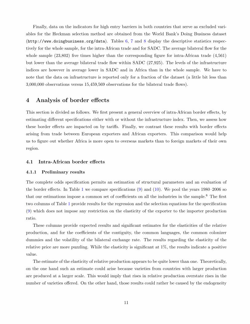
Finally, data on the indicators for high entry barriers in both countries that serve as excluded vari-

ables for the Heckman selection method are obtained from the World Bank’s Doing Business dataset

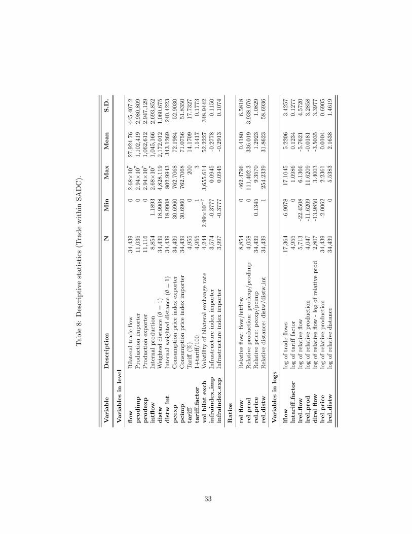
(http://www.doingbusiness.org/data). Tables 6, 7 and 8 display the descriptive statistics respec-

tively for the whole sample, for the intra-African trade and for SADC. The average bilateral flow for the

whole sample (23,802) five times higher than the corresponding figure for intra-African trade (4,561)

but lower than the average bilateral trade flow within SADC (27,925). The levels of the infrastructure

indices are however in average lower in SADC and in Africa than in the whole sample. We have to

note that the data on infrastructure is reported only for a fraction of the dataset (a little bit less than

3,000,000 observations versus 15,459,569 observations for the bilateral trade flows).

4 Analysis of border effects

This section is divided as follows. We first present a general overview of intra-African border effects, by

estimating different specifications either with or without the infrastructure index. Then, we assess how

these border effects are impacted on by tariffs. Finally, we contrast these results with border effects

arising from trade between European exporters and African exporters. This comparison would help

us to figure out whether Africa is more open to overseas markets than to foreign markets of their own

region.

4.1 Intra-African border effects

4.1.1 Preliminary results

The complete odds specification permits an estimation of structural parameters and an evaluation of

the border effects. In Table 1 we compare specifications (9) and (10). We pool the years 1980–2006 so

that our estimations impose a common set of coefficients on all the industries in the sample.8 The first

two columns of Table 1 provide results for the regression and the selection equations for the specification

(9) which does not impose any restriction on the elasticity of the exporter to the importer production

ratio.

These columns provide expected results and significant estimates for the elasticities of the relative

production, and for the coefficients of the contiguity, the common languages, the common colonizer

dummies and the volatility of the bilateral exchange rate. The results regarding the elasticity of the

relative price are more puzzling. While the elasticity is significant at 1%, the results indicate a positive

value.

The estimate of the elasticity of relative production appears to be quite lower than one. Theoretically,

on the one hand such an estimate could arise because varieties from countries with larger production

are produced at a larger scale. This would imply that rises in relative production overstate rises in the

number of varieties offered. On the other hand, those results could rather be caused by the endogeneity

11

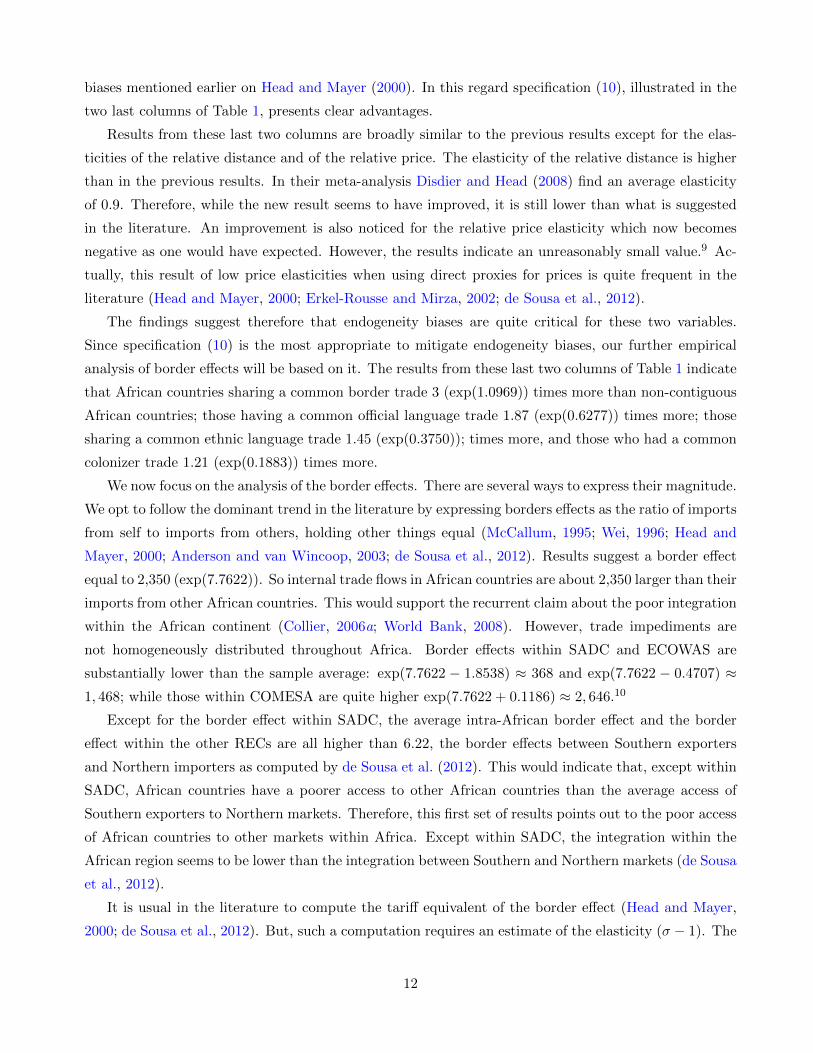
biases mentioned earlier on Head and Mayer (2000). In this regard specification (10), illustrated in the

two last columns of Table 1, presents clear advantages.

Results from these last two columns are broadly similar to the previous results except for the elas-

ticities of the relative distance and of the relative price. The elasticity of the relative distance is higher

than in the previous results. In their meta-analysis Disdier and Head (2008) find an average elasticity

of 0.9. Therefore, while the new result seems to have improved, it is still lower than what is suggested

in the literature. An improvement is also noticed for the relative price elasticity which now becomes

negative as one would have expected. However, the results indicate an unreasonably small value.9 Ac-

tually, this result of low price elasticities when using direct proxies for prices is quite frequent in the

literature (Head and Mayer, 2000; Erkel-Rousse and Mirza, 2002; de Sousa et al., 2012).

The findings suggest therefore that endogeneity biases are quite critical for these two variables.

Since specification (10) is the most appropriate to mitigate endogeneity biases, our further empirical

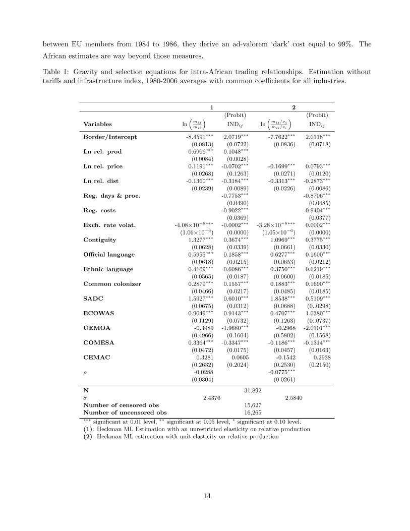
analysis of border effects will be based on it. The results from these last two columns of Table 1 indicate

that African countries sharing a common border trade 3 (exp(1.0969)) times more than non-contiguous

African countries; those having a common official language trade 1.87 (exp(0.6277)) times more; those

sharing a common ethnic language trade 1.45 (exp(0.3750)); times more, and those who had a common

colonizer trade 1.21 (exp(0.1883)) times more.

We now focus on the analysis of the border effects. There are several ways to express their magnitude.

We opt to follow the dominant trend in the literature by expressing borders effects as the ratio of imports

from self to imports from others, holding other things equal (McCallum, 1995; Wei, 1996; Head and

Mayer, 2000; Anderson and van Wincoop, 2003; de Sousa et al., 2012). Results suggest a border effect

equal to 2,350 (exp(7.7622)). So internal trade flows in African countries are about 2,350 larger than their

imports from other African countries. This would support the recurrent claim about the poor integration

within the African continent (Collier, 2006a; World Bank, 2008). However, trade impediments are

not homogeneously distributed throughout Africa. Border effects within SADC and ECOWAS are

substantially lower than the sample average: exp(7.7622 − 1.8538) ≈ 368 and exp(7.7622 − 0.4707) ≈1, 468; while those within COMESA are quite higher exp(7.7622 + 0.1186) ≈ 2, 646.10

Except for the border effect within SADC, the average intra-African border effect and the border

effect within the other RECs are all higher than 6.22, the border effects between Southern exporters

and Northern importers as computed by de Sousa et al. (2012). This would indicate that, except within

SADC, African countries have a poorer access to other African countries than the average access of

Southern exporters to Northern markets. Therefore, this first set of results points out to the poor access

of African countries to other markets within Africa. Except within SADC, the integration within the

African region seems to be lower than the integration between Southern and Northern markets (de Sousa

et al., 2012).

It is usual in the literature to compute the tariff equivalent of the border effect (Head and Mayer,

2000; de Sousa et al., 2012). But, such a computation requires an estimate of the elasticity (σ − 1). The

12

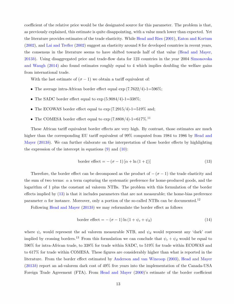
coefficient of the relative price would be the designated source for this parameter. The problem is that,

as previously explained, this estimate is quite disappointing, with a value much lower than expected. Yet

the literature provides estimates of the trade elasticity. While Head and Ries (2001), Eaton and Kortum

(2002), and Lai and Trefler (2002) suggest an elasticity around 8 for developed countries in recent years,

the consensus in the literature seems to have shifted towards half of that value (Head and Mayer,

2013b). Using disaggregated price and trade-flow data for 123 countries in the year 2004 Simonovska

and Waugh (2014) also found estimates roughly equal to 4 which implies doubling the welfare gains

from international trade.

With the last estimate of (σ − 1) we obtain a tariff equivalent of:

• The average intra-African border effect equal exp (7.7622/4)-1=596%;

• The SADC border effect equal to exp (5.9084/4)-1=338%;

• The ECOWAS border effect equal to exp (7.2915/4)-1=519% and;

• The COMESA border effect equal to exp (7.8808/4)-1=617%.11

These African tariff equivalent border effects are very high. By contrast, those estimates are much

higher than the corresponding EU tariff equivalent of 99% computed from 1984 to 1986 by Head and

Mayer (2013b). We can further elaborate on the interpretation of those border effects by highlighting

the expression of the intercept in equations (9) and (10):

border effect = − (σ − 1) [α+ ln (1 + ξ)] (13)

Therefore, the border effect can be decomposed as the product of − (σ − 1) the trade elasticity and

the sum of two terms: α a term capturing the systematic preference for home-produced goods, and the

logarithm of 1 plus the constant ad valorem NTBs. The problem with this formulation of the border

effects implied by (13) is that it includes parameters that are not measurable; the home-bias preference

parameter α for instance. Moreover, only a portion of the so-called NTBs can be documented.12

Following Head and Mayer (2013b) we may reformulate the border effect as follows

border effect = − (σ − 1) ln (1 + ψc + ψd) (14)

where ψc would represent the ad valorem measurable NTB, and ψd would represent any ‘dark’ cost

implied by crossing borders.13 From this formulation we can conclude that ψc + ψd would be equal to

596% for intra-African trade, to 338% for trade within SADC, to 519% for trade within ECOWAS and

to 617% for trade within COMESA. These figures are considerably higher than what is reported in the

literature. From the border effect estimated by Anderson and van Wincoop (2003), Head and Mayer

(2013b) report an ad-valorem dark cost of 49% five years into the implementation of the Canada-USA

Foreign Trade Agreement (FTA). From Head and Mayer (2000)’s estimate of the border coefficient

13

between EU members from 1984 to 1986, they derive an ad-valorem ‘dark’ cost equal to 99%. The

African estimates are way beyond those measures.

Table 1: Gravity and selection equations for intra-African trading relationships. Estimation withouttariffs and infrastructure index, 1980-2006 averages with common coefficients for all industries.

1 2

(Probit) (Probit)

Variables ln(mij

mii

)INDij ln

(mij/νjmii/νi

)INDij

Border/Intercept -8.4591∗∗∗ 2.0719∗∗∗ -7.7622∗∗∗ 2.0118∗∗∗

(0.0813) (0.0722) (0.0836) (0.0718)Ln rel. prod 0.6906∗∗∗ 0.1048∗∗∗

(0.0084) (0.0028)Ln rel. price 0.1191∗∗∗ -0.0702∗∗∗ -0.1699∗∗∗ 0.0793∗∗∗

(0.0268) (0.1263) (0.0271) (0.0120)Ln rel. dist -0.1360∗∗∗ -0.3184∗∗∗ -0.3313∗∗∗ -0.2873∗∗∗

(0.0239) (0.0089) (0.0226) (0.0086)Reg. days & proc. -0.7753∗∗∗ -0.8706∗∗∗

(0.0490) (0.0485)Reg. costs -0.9022∗∗∗ -0.9404∗∗∗

(0.0369) (0.0377)Exch. rate volat. -4.08×10−6∗∗∗ -0.0002∗∗∗ -3.28×10−6∗∗∗ 0.0002∗∗∗

(1.06×10−6) (0.0000) (1.05×10−6) (0.0000)Contiguity 1.3277∗∗∗ 0.3674∗∗∗ 1.0969∗∗∗ 0.3775∗∗∗

(0.0628) (0.0339) (0.0661) (0.0330)Official language 0.5955∗∗∗ 0.1858∗∗∗ 0.6277∗∗∗ 0.1600∗∗∗

(0.0618) (0.0215) (0.0653) (0.0212)Ethnic language 0.4109∗∗∗ 0.6086∗∗∗ 0.3750∗∗∗ 0.6219∗∗∗

(0.0565) (0.0187) (0.0600) (0.0185)Common colonizer 0.2879∗∗∗ 0.1557∗∗∗ 0.1883∗∗∗ 0.1690∗∗∗

(0.0466) (0.0217) (0.0485) (0.0185)SADC 1.5927∗∗∗ 0.6010∗∗∗ 1.8538∗∗∗ 0.5109∗∗∗

(0.0675) (0.0312) (0.0688) (0..0298)ECOWAS 0.9049∗∗∗ 0.9143∗∗∗ 0.4707∗∗∗ 1.0380∗∗∗

(0.1129) (0.0732) (0.1263) (0..0737)UEMOA -0.3989 -1.9680∗∗∗ -0.2968 -2.0101∗∗∗

(0.4966) (0.1604) (0.5802) (0.1568)COMESA 0.3364∗∗∗ -0.3347∗∗∗ -0.1186∗∗∗ -0.1314∗∗∗

(0.0472) (0.0175) (0.0457) (0.0163)CEMAC 0.3281 0.0605 -0.1542 0.2938

(0.2632) (0.2024) (0.2530) (0.2150)ρ -0.0288 -0.0775∗∗∗

(0.0304) (0.0261)

N 31,892σ 2.4376 2.5840Number of censored obs 15,627Number of uncensored obs 16,265∗∗∗ significant at 0.01 level, ∗∗ significant at 0.05 level, ∗ significant at 0.10 level.(1): Heckman ML Estimation with an unrestricted elasticity on relative production(2): Heckman ML estimation with unit elasticity on relative production

14

4.1.2 Accounting for infrastructure

We may need some less conventional sources of resistance to improve the estimates of the border effects

arising in intra-African trade.14 The usual sources of resistance – cross border tariffs or border compli-

ance costs – are not sufficient to explain the high level of border effects within Africa. Quoting Gross-

man (1998), Head and Mayer (2013b) mention three possible explanations: informational impediments

to trade, localized and historically determined tastes, and business networks. It is quite difficult to get

proxies for these dimensions, especially for intra-African trade. However, by using the infrastructure

indices of the importer and the exporter together, we might get an imperfect but useful proxy of the

business network which might be insightful for explaining the relatively low border resistance prevailing

in SADC.

While one might conjecture that SADC has established more effective institutions to promote re-

gional integration, another plausible explanation may emerge: the high quality of the transport infras-

tructure of several SADC countries (South Africa, Botswana, Namibia) may favor trade flows within

the region. It would be useful to use data on quality of transport-related infrastructure to disentangle

the impact of the infrastructure from the border effects.

The last two columns of Table 2 provide results with the infrastructure index. The first two columns

of the same table serve as a benchmark as they provide estimations with the same sample as with

the last two but without the infrastructure index. With the inclusion of the infrastructure index the

sample size drops significantly from 31,892 to 10,136. This drop of the sample size has an impact on

the elasticity of relative price and on the coefficient of the ethnic language dummy which now become

insignificant. Yet, we obtain a distance elasticity of about -0.8097, which suggests that the inclusion of

the infrastructure indices allow the distance elasticity to increase towards the estimate reported by Dis-

dier and Head (2008). Furthermore, with the infrastructure indices we find that contiguous countries

trade 1.73 (exp(0.5496)) more, countries sharing a common official language trade 2.04 (exp(0.7110))

more, and countries who had a common colonizer trade 1.73 (exp(0.5504)) more.

The impact of the infrastructure indices on the intra-African border effects is even more remarkable.

While the average intra-African border effects arising from the first two columns of Table 2 is about

2,750 (exp(7.9192)), it shrinks to 108 (exp(4.6806)) when the infrastructure indices of the importer and

the exporter are taken into account. Considering the infrastructure index implies a sharp decrease in

the average intra-African border effects. Actually this figure implies that internal trade flows in African

countries are about 108 larger than their imports from other African countries, after controlling for

distances, languages, contiguity effects, common colonizer effects, and infrastructure.

It is even more interesting to assess the border effects within the different regional groupings. With

respectively 22 (exp(4.6806-1.6053)), 33 (exp(4.6806-1.1861)) and 87 (exp(4.6806-0.2111)), the border

effects in SADC and ECOWAS are as before significantly lower than the continental average; while those

of COMESA are only slightly smaller. Therefore, after accounting for bilateral tariffs by deducting the

simple average world tariff (12.5%) the tariff equivalent of the sum of ‘grey’ and ‘dark’ costs becomes:

15

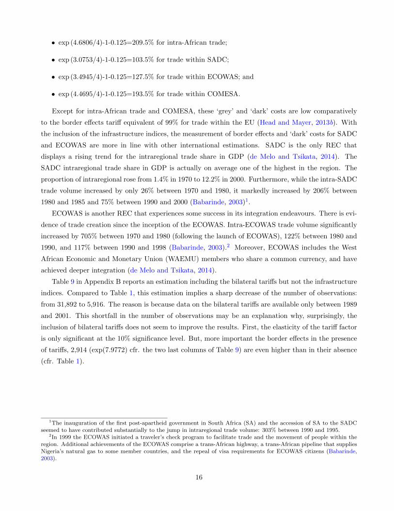
• exp (4.6806/4)-1-0.125=209.5% for intra-African trade;

• exp (3.0753/4)-1-0.125=103.5% for trade within SADC;

• exp (3.4945/4)-1-0.125=127.5% for trade within ECOWAS; and

• exp (4.4695/4)-1-0.125=193.5% for trade within COMESA.

Except for intra-African trade and COMESA, these ‘grey’ and ‘dark’ costs are low comparatively

to the border effects tariff equivalent of 99% for trade within the EU (Head and Mayer, 2013b). With

the inclusion of the infrastructure indices, the measurement of border effects and ‘dark’ costs for SADC

and ECOWAS are more in line with other international estimations. SADC is the only REC that

displays a rising trend for the intraregional trade share in GDP (de Melo and Tsikata, 2014). The

SADC intraregional trade share in GDP is actually on average one of the highest in the region. The

proportion of intraregional rose from 1.4% in 1970 to 12.2% in 2000. Furthermore, while the intra-SADC

trade volume increased by only 26% between 1970 and 1980, it markedly increased by 206% between

1980 and 1985 and 75% between 1990 and 2000 (Babarinde, 2003)1.

ECOWAS is another REC that experiences some success in its integration endeavours. There is evi-

dence of trade creation since the inception of the ECOWAS. Intra-ECOWAS trade volume significantly

increased by 705% between 1970 and 1980 (following the launch of ECOWAS), 122% between 1980 and

1990, and 117% between 1990 and 1998 (Babarinde, 2003).2 Moreover, ECOWAS includes the West

African Economic and Monetary Union (WAEMU) members who share a common currency, and have

achieved deeper integration (de Melo and Tsikata, 2014).

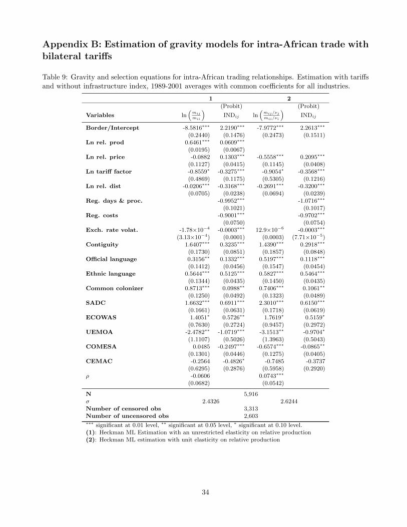
Table 9 in Appendix B reports an estimation including the bilateral tariffs but not the infrastructure

indices. Compared to Table 1, this estimation implies a sharp decrease of the number of observations:

from 31,892 to 5,916. The reason is because data on the bilateral tariffs are available only between 1989

and 2001. This shortfall in the number of observations may be an explanation why, surprisingly, the

inclusion of bilateral tariffs does not seem to improve the results. First, the elasticity of the tariff factor

is only significant at the 10% significance level. But, more important the border effects in the presence

of tariffs, 2,914 (exp(7.9772) cfr. the two last columns of Table 9) are even higher than in their absence

(cfr. Table 1).

1The inauguration of the first post-apartheid government in South Africa (SA) and the accession of SA to the SADCseemed to have contributed substantially to the jump in intraregional trade volume: 303% between 1990 and 1995.

2In 1999 the ECOWAS initiated a traveler’s check program to facilitate trade and the movement of people within theregion. Additional achievements of the ECOWAS comprise a trans-African highway, a trans-African pipeline that suppliesNigeria’s natural gas to some member countries, and the repeal of visa requirements for ECOWAS citizens (Babarinde,2003).

16

Table 2: Gravity and selection equations for intra-African trading relationships. Estimation with in-frastructure indices but without tariffs, 1980-2006 averages with common coefficients for all industriesand with unit production elasticity.

1 2

(Probit) (Probit)

Variables ln(mij/νjmii/νi

)INDij ln

(mij/νjmii/νi

)INDij

Border/Intercept -7.9192∗∗∗ 1.9563∗∗∗ -4.6806∗∗∗ 2.7636∗∗∗

(0.1343) (0.1321) (0.2192) (0.1778)Ln rel. price 0.0362 0.0024 0.0019 -0.0059

(0.0321) (0.0177) (0.0310) (0.0181)Ln rel. dist. -0.2954∗∗∗ -0.2059∗∗∗ -0.8097∗∗∗ -0.2888∗∗∗

(0.0322) (0.0156) (0.0377) (0.0212)Reg. days & proc. -0.5173∗∗∗ -0.4842∗∗∗

(0.07543) (0.0776)Reg. costs -0.9383∗∗∗ -0.6424∗∗∗

(0.0813) (0.0900)Exch. rate volat. -4.08×10−6∗∗∗ 6.41×10−5∗∗∗ -3.51×10−6∗∗∗ 8.45×10−5∗∗∗

(1.24×10−6) (1.71×10−5) (1.19×10−6) (0.000022)Contiguity 0.9570∗∗∗ 0.2900∗∗∗ 0.5496∗∗∗ 0.1655∗

(0.0962) (0.0968) (0.0965) (0.0949)Official language 0.9349∗∗∗ 0.4310∗∗∗ 0.7110∗∗∗ 0.3639∗∗∗

(0.1076) (0.0516) (0.1038) (0.0545)Ethnic language 0.1031 0.3990∗∗∗ 0.1438 0.4072∗∗∗

(0.1024) (0.0403) (0.0994) (0.0407)Common colonizer 0.1524∗∗ 0.1355∗∗∗ 0.5504∗∗∗ 0.2135∗∗∗

(0.0650) (0.0472) (0.0670) (0.0500)Ln infra index imp 5.3044∗∗∗ 0.7778∗∗∗

(0.2565) (0.1512)Ln infra index exp 1.0412∗∗∗ 1.4672∗∗∗

(0.2237) (0.1507)SADC 1.8323∗∗∗ 0.9671∗∗∗ 1.6053∗∗∗ 0.8661∗∗∗

(0.1338) (0.2225) (0.1255) (0.2187)ECOWAS 0.7495∗∗∗ 0.7680∗∗∗ 1.1861∗∗∗ 0.8374∗∗∗

(0.2295) (0.1941) (0.2192) (0.2020)COMESA -0.0589 0.1794∗∗∗ 0.2111∗∗∗ 0.1746∗∗∗

(0.0595) (0.0321) (0.0587) (0.0328)CEMAC 0.1627 -0.1395 0.4885∗ -0.0313

(0.2811) (0.2237) (0.2795) (0.2259)ρ -0.2741∗∗∗ 0.1208∗∗∗

(0.0614) (0.0345)

N 10,136σ 2.4626 2.3724Number of censored obs 2,288Number of uncensored obs 7,848∗∗∗ significant at 0.01 level, ∗∗ significant at 0.05 level, ∗ significant at 0.10 level.Heckman ML Estimations with an unrestricted elasticity on relative production

17

4.1.3 The impact of bilateral tariffs

The joint inclusion of bilateral tariffs and infrastructure indices (cfr. Table 10 in Appendix B) does

not bring much of an improvement. This joint inclusion reduces the sample size to 1,616 observations.

While the implied border effects 1,582 (exp(7.3662)), are lower than in Table 9, they are still much

higher than in the results derived from the specification with infrastructure indices but without tariffs

(displayed in Table 2).

The evolution of the border effects through time is analyzed next. Whether we include infrastructure

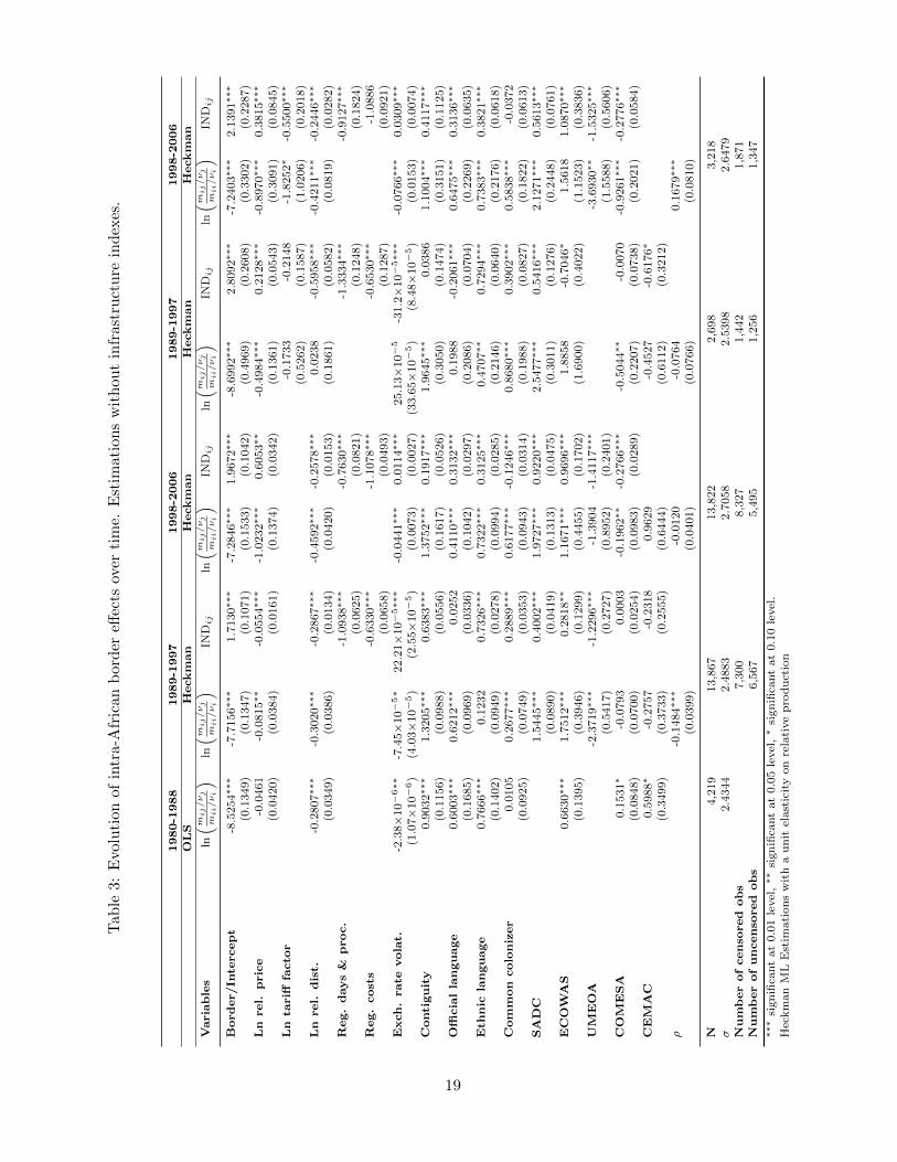
indices or not, two opposite outcomes emerge from this analysis. In Table 3 we can see the evolution

of border effects without accounting for infrastructure indices. The first five columns of Table 3 shows

the evolution when tariffs are not accounted for. We can notice there that border effects decreased from

5,041 (exp(8.5254)) between 1980-1988 to 2,243 (exp(7.7156)) between 1989-1997, and finally to 1,458

(exp(7.2846)). For SADC the border effects also decreased 479 (exp(7.7156-1.5445)) between 1989-1997

to 203 (exp(7.2846-1.9727)) between 1998-2006. Regarding ECOWAS, border effects decrease from

2,598 (exp(8.5254-0.6630)) between 1980-1988 to 389 (exp(7.7156-1.7512)) between 1989-1997 but then

increased slightly to 454 (exp(7.2846-1.1671)) between 1998-2006.

When we take tariffs into consideration, as in the last four columns of Table 3, border effects

also diminished from 5,998 (exp(8.6992)) between 1989-1997 to 1,395 (exp(7.2403)) between 1998-2006.

For SADC they also decreased from 469 (exp(8.6992-2.5477)) between 1989-1997 to 166 (exp(7.2403-

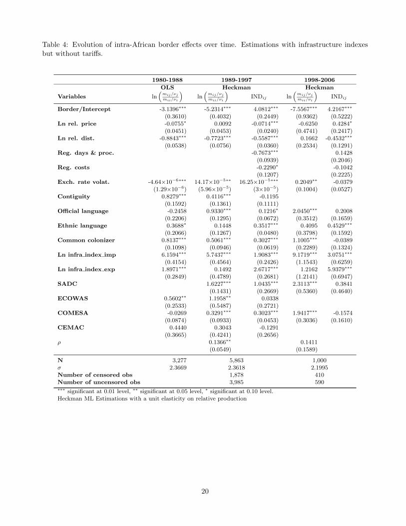
2.1271)). Let us now focus on the results with infrastructure indices. In doing so we disregard the

impact of bilateral tariffs. In this configuration, border effects evolve in the opposite direction. Table 4

shows the evolution of border effects when the infrastructure indices are included as regressors. Border

effects rise from 23 (exp(3.1396)) between 1980-1988 to 187 (exp(5.2314)) and to 1,914 (exp(7.5567)).

For SADC border effects increase from 37 (exp(5.2314-1.6227)) between 1989-1997 to 190 (exp(7.5567-

2.3113)) between 1998-2006.

The fact that tables 3 and 4 display evolutions in opposite direction might give ground to the

hypothesis that the decline of border effects is mostly driven by the improvement of transport and

communication infrastructure than by the reduction of NTBs like quotas, export restraints and s forth.

However, more information especially on NTBs is needed to confirm this suggestion.

18

Tab

le3:

Evolu

tion

ofin

tra-

Afr

ican

bor

der

effec

tsov

erti

me.

Est

imat

ion

sw

ithou

tin

frast

ruct

ure

ind

exes

.

1980-1

988

1989-1

997

1998-2

006

1989-1

997

1998-2

006

OL

SH

eckm

an

Heckm

an

Heckm

an

Heckm

an

Varia

ble

sln

( m ij/νj

mii/νi

)ln

( m ij/νj

mii/νi

)IN

Dij

ln( m i

j/νj

mii/νi

)IN

Dij

ln( m i

j/νj

mii/νi

)IN

Dij

ln( m i

j/νj

mii/νi

)IN

Dij

Bord

er/In

tercep

t-8

.5254∗∗∗

-7.7

156∗∗∗

1.7

130∗∗∗

-7.2

846∗∗∗

1.9

672∗∗∗

-8.6

992∗∗∗

2.8

092∗∗∗

-7.2

403∗∗∗

2.1

391∗∗∗

(0.1

349)

(0.1

347)

(0.1

071)

(0.1

533)

(0.1

042)

(0.4

969)

(0.2

608)

(0.3

302)

(0.2

287)

Ln

rel.

pric

e-0

.0461

-0.0

815∗∗

-0.0

554∗∗∗

-1.0

232∗∗∗

0.6

053∗∗

-0.4

984∗∗∗

0.2

128∗∗∗

-0.8

970∗∗∗

0.3

815∗∗∗

(0.0

420)

(0.0

384)

(0.0

161)

(0.1

374)

(0.0

342)

(0.1

361)

(0.0

543)

(0.3

091)

(0.0

845)

Ln

tariff

facto

r-0

.1733

-0.2

148

-1.8

252∗

-0.5

500∗∗∗

(0.5

262)

(0.1

587)

(1.0

206)

(0.2

018)

Ln

rel.

dis

t.-0

.2807∗∗∗

-0.3

020∗∗∗

-0.2

867∗∗∗

-0.4

592∗∗∗

-0.2

578∗∗∗

0.0

238

-0.5

958∗∗∗

-0.4

211∗∗∗

-0.2

446∗∗∗

(0.0

349)

(0.0

386)

(0.0

134)

(0.0

420)

(0.0

153)

(0.1

861)

(0.0

582)

(0.0

819)

(0.0

282)

Reg.

days

&p

roc.

-1.0

938∗∗∗

-0.7

630∗∗∗

-1.3

334∗∗∗

-0.9

127∗∗∗

(0.0

625)

(0.0

821)

(0.1

248)

(0.1

824)

Reg.

cost

s-0

.6330∗∗∗

-1.1

078∗∗∗

-0.6

530∗∗∗

-1.0

886

(0.0

658)

(0.0

493)

(0.1

287)

(0.0

921)

Exch

.rate

vola

t.-2

.38×

10−6∗∗

-7.4

5×

10−5∗

22.2

1×

10−5∗∗∗

-0.0

441∗∗∗

0.0

114∗∗∗

25.1

3×

10−5

-31.2×

10−5∗∗∗

-0.0

766∗∗∗

0.0

309∗∗∗

(1.0

7×

10−6)

(4.0

3×

10−5)

(2.5

5×

10−5)

(0.0

073)

(0.0

027)

(33.6

5×

10−5)

(8.4

8×

10−5)

(0.0

153)

(0.0

074)

Conti

gu

ity

0.9

032∗∗∗

1.3

205∗∗∗

0.6

383∗∗∗

1.3

752∗∗∗

0.1

917∗∗∗

1.9

645∗∗∗

0.0

386

1.1

004∗∗∗

0.4

117∗∗∗

(0.1

156)

(0.0

988)

(0.0

556)

(0.1

617)

(0.0

526)

(0.3

050)

(0.1

474)

(0.3

151)

(0.1

125)

Offi

cia

lla

ngu

age

0.6

003∗∗∗

0.6

212∗∗∗

0.0

252

0.4

110∗∗∗

0.3

132∗∗∗

0.1

988

-0.2

061∗∗∗

0.6

475∗∗∗

0.3

136∗∗∗

(0.1

685)

(0.0

969)

(0.0

336)

(0.1

042)

(0.0

297)

(0.2

086)

(0.0

704)

(0.2

269)

(0.0

635)

Eth

nic

lan

gu

age

0.7

666∗∗∗

0.1

232

0.7

326∗∗∗

0.7

322∗∗∗

0.3

125∗∗∗

0.4

707∗∗

0.7

294∗∗∗

0.7

383∗∗∗

0.3

821∗∗∗

(0.1

402)

(0.0

949)

(0.0

278)

(0.0

994)

(0.0

285)

(0.2

146)

(0.0

640)

(0.2

176)

(0.0

618)

Com

mon

colo

niz

er

0.0

105

0.2

677∗∗∗

0.2

889∗∗∗

0.6

177∗∗∗

-0.1

246∗∗∗

0.8

680∗∗∗

0.3

902∗∗∗

0.5

838∗∗∗

-0.0

372

(0.0

925)

(0.0

749)

(0.0

353)

(0.0

943)

(0.0

314)

(0.1

988)

(0.0

827)

(0.1

822)

(0.0

613)

SA

DC

1.5

445∗∗∗

0.4

002∗∗∗

1.9

727∗∗∗

0.9

220∗∗∗

2.5

477∗∗∗

0.5

416∗∗∗

2.1

271∗∗∗

0.5

613∗∗∗

(0.0

890)

(0.0

419)

(0.1

313)

(0.0

475)

(0.3

011)

(0.1

276)

(0.2

448)

(0.0

761)

EC

OW

AS

0.6

630∗∗∗

1.7

512∗∗∗

0.2

818∗∗

1.1

671∗∗∗

0.9

696∗∗∗

1.8

858

-0.7

046∗

1.5

618

1.0

870∗∗∗

(0.1

395)

(0.3

946)

(0.1

299)

(0.4

455)

(0.1

702)

(1.6

900)

(0.4

022)

(1.1

523)

(0.3

836)

UM

EO

A-2

.3719∗∗∗

-1.2

296∗∗∗

-1.3

904

-1.4

117∗∗∗

-3.6

930∗∗

-1.5

325∗∗∗

(0.5

417)

(0.2

727)

(0.8

952)

(0.2

401)

(1.5

588)

(0.5

606)

CO

ME

SA

0.1

531∗

-0.0

793

0.0

003

-0.1

962∗∗

-0.2

766∗∗∗

-0.5

044∗∗

-0.0

070

-0.9

261∗∗∗

-0.2

776∗∗∗

(0.0

848)

(0.0

700)

(0.0

254)

(0.0

983)

(0.0

289)

(0.2

207)

(0.0

738)

(0.2

021)

(0.0

584)

CE

MA

C0.5

988∗

-0.2

757

-0.2

318

0.9

629

-0.4

527

-0.6

176∗

(0.3

499)

(0.3

733)

(0.2

555)

(0.6

444)

(0.6

112)

(0.3

212)

ρ-0

.1484∗∗∗

-0.0

120

-0.0

764

0.1

679∗∗∗

(0.0

399)

(0.0

401)

(0.0

766)

(0.0

810)

N4,2

19

13,8

67

13,8

22

2,6

98

3,2

18

σ2.4

344

2.4

883

2.7

058

2.5

398

2.6

479

Nu

mb

er

of

cen

sored

ob

s7,3

00

8,3

27

1,4

42

1,8

71

Nu

mb

er

of

uncenso

red

ob

s6,5

67

5,4

95

1,2

56

1,3

47

∗∗∗

sign

ifica

nt

at

0.0

1le

vel

,∗∗

sign

ifica

nt

at

0.0

5le

vel

,∗

sign

ifica

nt

at

0.1

0le

vel

.H

eckm

an

ML

Est

imati

on

sw

ith

au

nit

elast

icit

yon

rela

tive

pro

du

ctio

n

19

Table 4: Evolution of intra-African border effects over time. Estimations with infrastructure indexesbut without tariffs.

1980-1988 1989-1997 1998-2006

OLS Heckman Heckman

Variables ln(mij/νjmii/νi

)ln

(mij/νjmii/νi

)INDij ln

(mij/νjmii/νi

)INDij

Border/Intercept -3.1396∗∗∗ -5.2314∗∗∗ 4.0812∗∗∗ -7.5567∗∗∗ 4.2167∗∗∗

(0.3610) (0.4032) (0.2449) (0.9362) (0.5222)Ln rel. price -0.0755∗ 0.0092 -0.0714∗∗∗ -0.6250 0.4284∗

(0.0451) (0.0453) (0.0240) (0.4741) (0.2417)Ln rel. dist. -0.8843∗∗∗ -0.7723∗∗∗ -0.5587∗∗∗ 0.1662 -0.4532∗∗∗

(0.0538) (0.0756) (0.0360) (0.2534) (0.1291)Reg. days & proc. -0.7673∗∗∗ 0.1428

(0.0939) (0.2046)Reg. costs -0.2290∗ -0.1042

(0.1207) (0.2225)Exch. rate volat. -4.64×10−6∗∗∗ 14.17×10−5∗∗ 16.25×10−5∗∗∗ 0.2049∗∗ -0.0379

(1.29×10−6) (5.96×10−5) (3×10−5) (0.1004) (0.0527)Contiguity 0.8279∗∗∗ 0.4116∗∗∗ -0.1195

(0.1592) (0.1361) (0.1111)Official language -0.2458 0.9330∗∗∗ 0.1216∗ 2.0450∗∗∗ 0.2008

(0.2206) (0.1295) (0.0672) (0.3512) (0.1659)Ethnic language 0.3688∗ 0.1448 0.3517∗∗∗ 0.4095 0.4529∗∗∗

(0.2066) (0.1267) (0.0480) (0.3798) (0.1592)Common colonizer 0.8137∗∗∗ 0.5061∗∗∗ 0.3027∗∗∗ 1.1005∗∗∗ -0.0389

(0.1098) (0.0946) (0.0619) (0.2289) (0.1324)Ln infra index imp 6.1594∗∗∗ 5.7437∗∗∗ 1.9083∗∗∗ 9.1719∗∗∗ 3.0751∗∗∗

(0.4154) (0.4564) (0.2426) (1.1543) (0.6259)Ln infra index exp 1.8971∗∗∗ 0.1492 2.6717∗∗∗ 1.2162 5.9379∗∗∗

(0.2849) (0.4789) (0.2681) (1.2141) (0.6947)SADC 1.6227∗∗∗ 1.0435∗∗∗ 2.3113∗∗∗ 0.3841

(0.1431) (0.2669) (0.5360) (0.4640)ECOWAS 0.5602∗∗ 1.1958∗∗ 0.0338

(0.2533) (0.5487) (0.2721)COMESA -0.0269 0.3291∗∗∗ 0.3023∗∗∗ 1.9417∗∗∗ -0.1574

(0.0874) (0.0933) (0.0453) (0.3036) (0.1610)CEMAC 0.4440 0.3043 -0.1291

(0.3665) (0.4241) (0.2656)ρ 0.1366∗∗ 0.1411

(0.0549) (0.1589)

N 3,277 5,863 1,000σ 2.3669 2.3618 2.1995Number of censored obs 1,878 410Number of uncensored obs 3,985 590∗∗∗ significant at 0.01 level, ∗∗ significant at 0.05 level, ∗ significant at 0.10 level.Heckman ML Estimations with a unit elasticity on relative production

20

4.2 Intra-African border effects vs Europe-Africa border effects

Table 5 provides results of the estimation of the specification (10) for exports from Europe to Africa. The

first two columns report results without the infrastructure indices, while the last two columns display

results accounting for them. Before commenting on the border effects that apply to European exports

in Africa, let us discuss some of the other results. Few of them are actually noteworthy: countries

previously involved in a colonial relationship and those sharing a language spoken by at least 5% of the

population trade 3 (respectively exp(1.1116) and exp(1.0935)) times more than the sample average.

Surprisingly, memberships to free trade agreements linking African to European countries do not

seem to pay off. The coefficient of the dummy for the European Free Trade Association (EFTA)15 - the

Morocco free trade agreement - is not significant in any of the specifications of Table 5. The results for

Africa Caribbean Pacific (ACP)16 - European Union (EU) preferential trade agreement are even more

surprising: the dummy coefficient is negative. This is quite counter-intuitive as one would expect that

such a preferential trade agreement would boost trade rather than impede it.

According to the last two columns of Table 5 (with infrastructure indices), border effects faced by

European exporters in African countries can be estimated to be about 34 (exp(3.5130)). They are higher

than the average intra-African border effects (108) but lower than the SADC and the ECOWAS border

effects. Hence, while on average African countries seem more open to overseas trade flows than to those

coming from their regional partners, regional economic groupings like SADC and ECOWAS seem to be

more open to their intra-regional trade flows than to European exports. This finding is consistent with

earlier findings showing that, after accounting for the impact of infrastructure, SADC and ECOWAS

border effects get closer to international estimations.

21

Table 5: Gravity and selection equations for trading relationships between European exporters andAfrican importers. Estimation with infrastructure indexes but without tariffs, 1980-2006 averages withcommon coefficients for all industries and with unit production elasticity.

1 2

(Probit) (Probit)

Variables ln(mij/νjmii/νi

)INDij ln

(mij/νjmii/νi

)INDij

Border/Intercept -5.9305∗∗∗ 1.8329∗∗∗ -3.5130∗∗∗ 1.2862∗∗∗

(0.0532) (0.0416) (0.0793) (0.0671)Ln rel. price -0.0493∗ 0.3323∗∗∗ -0.0569∗∗∗ 0.1064∗∗∗

(0.0258) (0.0122) (0.0179) (0.0130)Ln rel. dist. -0.9245∗∗∗ -0.0338∗∗∗ -1.2948∗∗∗ -0.1152∗∗∗

(0.0143) (0.0077) (0.0145) (0.0114)Colonial relationship 1.5657∗∗∗ 1.0951∗∗∗ 1.1116∗∗∗ 1.0571∗∗∗

(0.0594) (0.1828) (0.0534) (0.1948)Col. relat. post 1945 -0.5757∗∗∗ 0.2312 1.76×10−5 0.2089

(0.0690) (0.2449) (0.0658) (0.2946)Reg. days & proc. -0.6434∗∗∗ -0.9358∗∗∗

(0.0379) (0.2031)Reg. costs -0.1241∗∗∗ -0.8478∗∗∗

(0.0201) (0.2217)Official language 0.1728∗∗ -0.4498∗∗∗ -0.5480∗∗∗ 0.0155

(0.0785) (0.0847) (0.0768) (0.1075)Ethnic language 0.4114∗∗∗ 0.4974∗∗∗ 1.0935∗∗∗ 0.2242∗∗

(0.0734) (0.0775) (0.0719) (0.1000)Ln infra index imp 5.5967∗∗∗ 1.1019∗∗∗

(0.1005) (0.0951)Ln infra index exp 0.5887∗∗∗ 1.8828∗∗∗

(0.0545) (0.0407)EFTA MOROCCO -0.0254 -1.0497∗∗∗ -0.4455 -0.8298∗∗

(0.5404) (0.3338) (0.4986) (0.3533)UE ACP -0.7418∗∗∗ 0.4686∗∗∗ -0.1584∗∗∗ 0.0074

(0.0313) (0.0218) (0.0286) (0.0218)ρ -0.6822∗∗∗ 0.0048

(0.0485) (0.0192)

N 42,936σ 2.3829 2.1496Number of censored obs 4,697Number of uncensored obs 38,239∗∗∗ significant at 0.01 level, ∗∗ significant at 0.05 level, ∗ significant at 0.10 level.Heckman ML Estimations with an unrestricted elasticity on relative production

22

5 Conclusion

The results show that on average the African continent is poorly integrated and more open to overseas

export than to intra-African trade flows. However, this negative picture is contrasted by the fact that

two African RECs, SADC and ECOWAS have border effects that are more in line with international

estimations. Hence, there is evidence that these two African RECs are effective in promoting intrare-

gional trade. RECs are expected to increase trade between their members via three channels. The

first is a reduction in tariffs between members; the second is a reduction in NTBs; the third is via the

two components of ‘trade facilitation’: a ‘hard’ component related to tangible transport and telecom-

munications infrastructure; and a ‘soft’ component related to transparency, the business environment,

customs management, and other intangible institutional aspects that may facilitate trading (de Melo

and Tsikata, 2014).

The first two channels are the outcomes of measures that are easier to implement and have generally

been undertaken even by the African RECs that only manage to achieve ‘shallow’ integration (de Melo

and Tsikata, 2014). However, the measures implied by the two components of ‘trade facilitation’ are

much more difficult to put in place. This is especially true for the infrastructure dimension. Our model

explicitly account for that ‘hard’ component. Considering infrastructure indices is an interesting way

to capture the effect of distribution networks which represent, along with imperfect information and

localized tastes, sources of resistance that are generally omitted and can possibly explain the counter-

intuitive high border effects (Head and Mayer, 2013b).

The elasticity of the infrastructure indices are high and significant, suggesting that improving trans-

port and telecommunications infrastructures will go a long way in promoting inter-African trade. So

far only Northern and Southern Africa are well endowed in this regard, and it is clear that building and

improving infrastructure in other parts of the continent will generate additional trade opportunities.

The ‘soft’ component of trade facilitation is likely to be the factor explaining the discrepancies between

the different African RECs in terms of border effects. In this regard SADC and ECOWAS seem to have

set institutions that are more effective in achieving trade integration and allow them to be one step

ahead comparatively to other African RECs.

Yet, even these two RECs are still behind Regional Trade Agreements (RTA) in other continents

in terms of the importance of intra-regional trade share in GDP. While the SADC intra-regional trade

share in GDP – on average one of the highest in the continent – rose from 6% to 11% from 1992 to 2013,

the share of intra-RTA trade worldwide, excluding the EU, increased from 18% in 1990 to 34% in 2008

(from 28% to 51% if EU included). So there is still room for improvement in African RECs regarding

this ‘soft’ component of trade facilitation. Actually, regional integration in Africa was based on the

‘linear model’ of integration, with a stepwise integration of goods, labour, and capital markets, as well

as eventual monetary and fiscal integration. Most of African countries overlooked the importance of

tackling ‘behind-the-border’ impediments to trade, yet this is crucial in global environment characterized

23

by the reduction in trade costs and the subsequent fragmentation of production (de Melo and Tsikata,

2014).

Based on our results, two propositions may help reduce border effects and increase inter-regional

trade in Africa. First is the development of large pan-African infrastructure projects which can con-

tribute to defragmenting Africa by decreasing transport costs. Second is the implementation of the

African free trade zone that might bring free trade among the members by: removing tariffs and NTBs

and implementing trade facilitation, by applying the subsidiarity principle to infrastructure to enhance

the transport network, and by fostering industrial development (de Melo and Tsikata, 2014). These

measures will allow African countries to achieve a ‘deep’ rather than a ‘shallow integration’.

Finally, we have to acknowledge the limitations of the study. The main challenges are the quality and

the availability of the African data. Ideally, anyone would have opted for a more direct way to capture

the impact of distribution networks. Combes et al. (2005) for instance examine the impact of business

and social networks on trade between French regions by using the financial structure and location of

French firms as well as the bilateral stocks of migrants. Moreover, Combes et al. (2005) also use data on

transport costs which allow them to separate the effects of transport infrastructure and administrative

border effects.

Another issue that we are facing is that we rely on data on trade flows between different countries.

This implies that in order to estimate border effects we cannot use LSDV estimation; we rely instead on

the complete odds specification which requires a measure of the trade of a country with itself (“trade

with self”). Generally, this “trade with self” is proxied by using production minus total exports. While,

the complete odds specification has been used by several papers (Head and Mayer, 2000; de Sousa et al.,

2012), the measure of “trade with self” may cause some measurement errors as the procedure may

generate some negative observations for some countries (Head and Mayer, 2013a). The ideal would be

to use databases on commodity flows like in Wolf (2000), Anderson and van Wincoop (2003), Hillberry

and Hummels (2003), and Combes et al. (2005) which include inter- and intraregional trade flows.

However, it can be argued that this kind of datasets represents the exception rather than the norm.

Moreover, in the current state of the data collection on African countries, it will be challenging to get

reliable data on the missing sources of resistance. Getting such data is yet the price to pay to improve

on the analysis of border effects in intra-African trade.

Acknowledgements. Alain Pholo Bala gratefully acknowledges financial support from Economic

Research Southern Africa (ersa), South Africa. The views expressed in this paper and any remaining

errors are ours.

Notes

1With data on inter-provincial trade flows, one can estimate the border effects with a fixed effects specification (Feenstra,

2004).

24

2 Head and Mayer (2013a) offers a more in-depth discussion of those models.3These results might be explained by the fact that in specifications (9) and (10), we are dealing with ratios of trade

flow from j to i to trade flow of i from “self” rather than trade flows per se.4Available through the following download page: http://

www.cepii.fr/anglaisgraph/bdd/TradeProd.htm. In this webpage it is recommended to cite de Sousa et al. (2012)’

reference as the source of the data.5One of the file of the GeoDist database, the dist cepii dataset contains 2 variables indicating whether two countries,

origin and destination, share a common official language, or a common ethnic language, i.e. a language that is spoken by

at least 9% of the population in both countries.6Details on the formulas of distw and distwces are given in Mayer and Zignago (2011, p. 11).7Infrastructure data may be found at the following link:

http://thedata.harvard.edu/dvn/dv/pep/faces/study/StudyPage.xhtml?globalId=hdl:1902.1/11953.8It would have been useful to estimate the gravity model separately for different industries as in Head and Mayer (2000)

and de Sousa et al. (2012), but then we would have ended up with small numbers of observations for some industries.9Head and Mayer (2000) suggest that those low estimates are due to the unobserved variation in relative product quality

which is correlated with relative product price.10Border effects within other African RECs are not statistically different from the sample average.11While for the second estimate, we would obtain a tariff equivalent respectively equal to exp (7.7622/8)-1=164% for

intra-African trade, exp (5.9084/8)-1=109% for SADC, exp (7.2915/8)-1=149% for ECOWAS andexp (7.8808/8)-1=168%

for COMESA. With the same value of the elasticity of trade with respect to trade costs, de Sousa et al. (2012) found a

tariff equivalent of 118% between Southern exporters and Northern importers. Not surprisingly this finding confirms the

previous finding that SADC is the only REC within Africa, where members have easier access to the markets of their

partners than to overseas markets.12While NTBs like quotas, voluntary export restraints and non-automatic import authorizations often have much more

significant effects, only a few databases provide information on non-tariff barriers (e.g. the Doing Business database, the

Trade Facilitation Database, the Logistic Performance Index, the UNCTAD/TRAINS NTM and the CEPII NTM-MAP

databases). The cause of the rarity of databases on NTBs is largely due to the difficulty in collecting the data and in

assembling a consistent cross-country dataset. Unlike tariffs, NTB data are not merely numbers; the relevant information

is often hidden in legal and regulatory documents. Furthermore, these documents are generally not centralized but often

reside in different regulatory agencies. All these issues make the collection of NTB data a very resource-intensive task.

The CEPII NTM-MAP database has been designed to address the shortcomings of the previous databases, yet its index

is only provided for 63 countries for one year over the period 2010-2012 at the country level and two different product

disaggregation levels. Moreover, only 15 African countries are included in the database (Gourdon, 2014).13The concept of ‘dark’ costs results from an analogy with the cosmology concept of dark energy or dark matter. Neither

dark energy nor dark matter can be observed directly, but their presence is inferred to be tremendous. Therefore, ‘dark’

costs represent unobserved or difficult-to-observe trade costs which imply a significant resistance to trade flows. More

information about the astrophysics analogy between ‘dark’ cost and dark energy or dark matter is available in Head and

Mayer (2013b).14The ‘dark’ costs computed by Head and Mayer (2013b) include everything other than tariffs. So they may capture

border compliance costs which may be evaluated (the so-called ‘grey’ costs ψc). Head and Mayer (2013b) acknowledge

that their presentation of the concept of dark costs missed that distinction. However, since they report custom clearance

costs which seem to be negligible (1.8% for EU, and 2.0%-3.4% for the Canada-USA frontier), the ‘dark’ costs seem to be

dominant. Eventually, while the specifications (9) and (10) account for bilateral tariffs, Table 1 does not. So we may still

need to deduct the bilateral tariffs from the estimated ‘dark’ costs. If we use the simple average world tariff (12.5%) as an

approximation (Head and Mayer, 2013b), the intra-African trade dark costs are only slightly affected.15The EFTA is an intergovernmental organization set up for the promotion of free trade and economic integration to

25

the benefit of its four Member States: Iceland, Liechtenstein, Norway, Switzerland (http://www.efta.int).16“The African, Caribbean and Pacific Group of States (ACP) is an organization created by the Georgetown Agree-

ment in 1975. It is composed of 79 African, Caribbean and Pacific states, with all of them, save Cuba, signatories

to the Cotonou Agreement, also known as the “ACP-EC Partnership Agreement” which binds them to the European

Union”(http://www.acp.int/content/secretariat-acp).

References

Ancharaz, V., Mbekeani, K. and Brixiova, Z. (2011), ‘Impediments to Regional Trade Integration in

Africa’, Africa Economic Brief 2(11).

Anderson, J. E. and van Wincoop, E. (2003), ‘Gravity with Gravitas: A Solution to the Border Puzzle’,

American Economic Review 93(1), 170–192.

Artadi, E. V. and Sala-i Martin, X. (2003), The Economic Tragedy of the XXth Century: Growth in

Africa, NBER Working Papers 9865, National Bureau of Economic Research, Inc.

Au, C.-C. and Henderson, J. V. (2006), ‘Are Chinese Cities Too Small?’, Review of Economic Studies

73(3), 549–576.

Babarinde, F. (2003), Regionalism and economic development, in E. U. Nnadozie, ed., ‘African economic

development’, Amsterdam : London : Academic, book; book/illustrated 19, pp. 473–497.

Baldwin, R. and Harrigan, J. (2011), ‘Zeros, Quality, and Space: Trade Theory and Trade Evidence’,

American Economic Journal: Microeconomics 3(2), 60–88.

Behrens, K., Ertur, C. and Koch, W. (2012), ‘Dual Gravity: Using Spatial Econometrics To Control

For Multilateral Resistance’, Journal of Applied Econometrics 27(5), 773–794.

Canning, D. (1998), ‘A database of world stocks of infrastructure, 195095’, The World Bank Economic

Review 12(3), 529–547.

Carrere, C. (2004), ‘African regional agreements: Impact on trade with or without currency unions’,

Journal of African Economies 13(2), 199–239.

Carrere, C. (2006), ‘Revisiting the effects of regional trade agreements on trade flows with proper

specification of the gravity model’, European Economic Review 50(2), 223–247.

Cinyabuguma, M. M. and Putterman, L. (2011), ‘Sub-Saharan Growth Surprises: Being Heterogeneous,

Inland and Close to the Equator Does not Slow Growth Within Africa-super- ’, Journal of African

Economies 20(2), 217–262.

Collier, P. (2006a), ‘Africa : geography and growth’, Proceedings - Economic Policy Symposium -

Jackson Hole pp. 235–252.

26

Collier, P. (2006b), ‘African Growth: Why a ‘Big Push’?’, Journal of African Economies 15(2), 188–211.

Combes, P.-P., Lafourcade, M. and Mayer, T. (2005), ‘The trade-creating effects of business and social

networks: evidence from france’, Journal of International Economics 66(1), 1 – 29.

de Melo, J. and Tsikata, Y. (2014), Regional integration in Africa: Challenges and prospects, Working

Papers P93, FERDI.

de Sousa, J., Mayer, T. and Zignago, S. (2012), ‘Market access in global and regional trade’, Regional

Science and Urban Economics 42(6), 1037–1052.

Disdier, A.-C. and Head, K. (2008), ‘The Puzzling Persistence of the Distance Effect on Bilateral Trade’,

The Review of Economics and Statistics 90(1), 37–48.

Dollar, D. and Easterly, W. (1999), ‘The Search for the Key: Aid, Investment and Policies in Africa’,

Journal of African Economies 8(4), 546–77.

Easterly, W. (2009a), ‘Can the West Save Africa?’, Journal of Economic Literature 47(2), 373–447.

Easterly, W. (2009b), ‘How the Millennium Development Goals are Unfair to Africa’, World Development

37(1), 26–35.

Easterly, W. and Levine, R. (1997), ‘Africa’s Growth Tragedy: Policies and Ethnic Divisions’, The

Quarterly Journal of Economics 112(4), 1203–50.

Eaton, J. and Kortum, S. (2001), ‘Trade in capital goods’, European Economic Review 45(7), 1195–1235.

Eaton, J. and Kortum, S. (2002), ‘Technology, Geography, and Trade’, Econometrica 70(5), 1741–1779.

Eaton, J., Kortum, S. S. and Sotelo, S. (2012), International Trade: Linking Micro and Macro, NBER

Working Papers 17864, National Bureau of Economic Research, Inc.

Eaton, J. and Tamura, A. (1994), ‘Bilateralism and Regionalism in Japanese and U.S. Trade and Direct

Foreign Investment Patterns’, Journal of the Japanese and International Economies 8(4), 478–510.

Economic Commission for Africa (2011), “Boosting Intra-African Trade”. Preparations for the 7th AU

Trade Ministers Conference and the 18th Ordinary Session of the AU Assembly of Heads of State and

Government, Issues paper, Economic Commission for Africa.

Erkel-Rousse, H. and Mirza, D. (2002), ‘Import price elasticities: reconsidering the evidence’, Canadian

Journal of Economics/Revue canadienne d’economique 35(2), 282–306.

Evans, C. L. (2003), ‘The Economic Significance of National Border Effects’, American Economic Review

93(4), 1291–1312.

27

Feenstra, R. C. (2004), Advanced international trade: theory and evidence, Princeton University Press.

Freire, M. E. M., Lall, S. and Leipziger, D. (2015), Africa’s urbanization: Challenges and opportunities,

in C. Monga and J. Y. Lin, eds, ‘The Oxford Handbook of Africa and Economics’, Vol. 1: Context

and Concepts, Oxford University Press, chapter 31, pp. 584–602.

Gourdon, J. (2014), CEPII NTM-MAP: A Tool for Assessing the Economic Impact of Non-Tariff Mea-

sures, Working Papers 2014-24, CEPII research center.

Grossman, G. M. (1998), Comment on: Determinants of Bilateral Trade: Does Gravity Work in a

Neoclassical World?, in J. A. Frankel, ed., ‘The Regionalization of the World Economy’, University

of Chicago Press, pp. 29–31.

Harrigan, J. (1996), ‘Openness to trade in manufactures in the OECD’, Journal of International Eco-

nomics 40(1-2), 23–39.

Head, K. and Mayer, T. (2000), ‘Non-Europe: The magnitude and causes of market fragmentation in

the EU’, Review of World Economics (Weltwirtschaftliches Archiv) 136(2), 284–314.

Head, K. and Mayer, T. (2013a), Gravity Equations: Workhorse,Toolkit, and Cookbook, Working

Papers 2013-27, CEPII research center.

Head, K. and Mayer, T. (2013b), ‘What separates us? sources of resistance to globalization’, Canadian

Journal of Economics/Revue canadienne d’conomique 46(4), 1196–1231.

Head, K. and Ries, J. (2001), ‘Increasing returns versus national product differentiation as an explana-

tion for the pattern of u.s.-canada trade’, American Economic Review 91(4), 858–876.

Helliwell, J. F. (1996), ‘Do National Borders Matter for Quebec’s Trade?’, Canadian Journal of Eco-

nomics 29(3), 507–22.

Helpman, E., Melitz, M. and Rubinstein, Y. (2008), ‘Estimating trade flows: Trading partners and

trading volumes’, The Quarterly Journal of Economics 123(2), 441–487.

Hillberry, R. (1998), ‘Regional trade and the medicine line: The national border effect in u.s. commodity

flow data’, Journal of Borderlands Studies 13(2), 1–17.

Hillberry, R. and Hummels, D. (2003), ‘Intranational Home Bias: Some Explanations’, The Review of

Economics and Statistics 85(4), 1089–1092.

Hummels, D. (1999), Toward a Geography of Trade Costs, GTAP Working Papers 1162, Center for

Global Trade Analysis, Department of Agricultural Economics, Purdue University.

ITC (2012), Africa’s Trade Potential: Export Opportunities in Growth Markets, International Trade

Centre (ITC).

28

Jones, B. (2002), ‘Economic integration and convergence of per capita income in west africa’, African

Development Review 14(1), 18–47.

Krugman, P. (1980), ‘Scale Economies, Product Differentiation, and the Pattern of Trade’, American

Economic Review 70(5), 950–59.

Lai, H. and Trefler, D. (2002), The Gains from Trade with Monopolistic Competition: Specification, Es-

timation, and Mis-Specification, NBER Working Papers 9169, National Bureau of Economic Research,

Inc.

Limao, N. and Venables, A. J. (2001), ‘Infrastructure, geographical disadvantage, transport costs, and

trade’, The World Bank Economic Review 15(3), 451–479.

Mayer, T. and Zignago, S. (2011), Notes on CEPIIs distances measures: The GeoDist database, Working

Papers 2011-25, CEPII research center.

McCallum, J. (1995), ‘National Borders Matter: Canada-U.S. Regional Trade Patterns’, American

Economic Review 85(3), 615–23.

Page, J. (2008), Rowing Against the Current: The Diversification Challenge in Africa’s Resource-Rich

Economies, Brookings Global Economy & Development Working Papers No. 28 December 2008.

Pinkovskiy, M. and Sala-i Martin, X. (2014), ‘Africa is on time’, Journal of Economic Growth 19(3), 311–

338.

Redding, S. and Venables, A. J. (2004), ‘Economic geography and international inequality’, Journal of

International Economics 62(1), 53–82.

Sachs, J. D. and Warner, A. M. (1997), ‘Sources of Slow Growth in African Economies’, Journal of

African Economies 6(3), 335–76.

Simonovska, I. and Waugh, M. E. (2014), ‘The elasticity of trade: Estimates and evidence’, Journal of

International Economics 92(1), 34 – 50.

UNECA (2010), Assessing Regional Integration in Africa IV: Enhancing Intra-African Trade, United

Nations Economic Commission for Africa.

Wei, S.-J. (1996), Intra-National versus International Trade: How Stubborn are Nations in Global

Integration?, NBER Working Papers 5531, National Bureau of Economic Research, Inc.

Wolf, H. C. (2000), ‘Intranational home bias in trade’, The Review of Economics and Statistics

82(4), 555–563.

World Bank (2006), World Development Indicators 2006, number 8151 in ‘World Bank Publications’,

The World Bank.

29

World Bank (2008), World Development Report 2009: Reshaping Economic Geography, World Bank.

30

Ap

pen

dix

A:

Desc

rip

tive

stati

stic

sof

conti

nu

ou

svari

ab

les

Tab

le6:

Des

crip

tive

stat

isti

cs(A

llsa

mp

le).

Vari

able

Desc

ripti

on

NM

inM

ax

Mean

S.D

.

Vari

able

sin

level

flow

Bilate

ral

trade

flow

15,4

59,5

69

05.8

5×

108

23,8

02.3

21,3

83,9

90

pro

dim

pP

roduct

ion

imp

ort

er6,4

96,3

23

06.3

9×

108

7,9

87,5

97

3.2

2×

107

pro

dexp

Pro

duct

ion

exp

ort

er6,8

14,0

40

06.3

9×

108

8,6

89,3

62

3.3

1×

107

intfl

ow

Inte

rnal

pro

duct

ion

5,2

84,6

01

0.1

547

5.8

2×

108

7,2

08,6

16

2.8

3×

107

dis

twW

eighte

ddis

tance

(θ=

1)

13,8

32,0

99

8.4

497

19,7

81.3

98,1

40.1

05

4,6

71.9

1dis

twin

tIn

tern

al

wei

ghte

ddis

tance

(θ=

1)

14,3

79,9

02

0.9

951

1,8

53.8

02

258.2

357

290.4

453

pcexp

Consu

mpti

on

pri

cein

dex

exp

ort

er13,0

38,9

51

4.6

107

10,5

57.4

963.1

952

49.9

450

pcim

pC

onsu

mpti

on

pri

cein

dex

imp

ort

er13,0

23,0

79

4.6

107

10,5

57.4

963.0

925

65.4

607

tari

ffT

ari

ff(%

)295,9

88

01,7

38.8

01

22.6

809

57.3

162

tari

fffa

cto

r1+

tari

ff/100

295,9

88

118.3

880

1.2

268

0.5

732

vol

bilat

exch

Vola

tility

of

bilate

ral

exch

ange

rate

59,1

66

0562,0

60.9

358.0

921

11,7

91.4

infr

ain

dex

imp

Infr

ast

ruct

ure

index

imp

ort

er2,8

43,9

38

-0.3

986

8.1

165

0.3

643

1.0

591

infr

ain

dex

exp

Infr

ast

ruct

ure

index

imp

ort

er2,9

11,3

19

-0.3

986

8.1

165

0.4

565

1.0

330

Rati

os

rel

flow

Rel

ati

ve

flow

:flow

/in

tflow

5,2

84,6

01

024,8

46.4

20.0

820

15.7

467

rel

pro

dR

elati

ve

pro

duct

ion:

pro

dex

p/pro

dim

p2,9

71,8

10

03.2

5×

108

2,5

34.2

46

254,3

62.9

rel

pri

ce

Rel

ati

ve

pri

ce:

pce

xp/p

cim

p10,8

53,0

16

0.0

017

602.6

09

1.2

392

1.2

182

rel

dis

twR

elati

ve

dis

tance

:dis

tw/dis

twin

t13,3

15,0

39

0.6

124

19,7

43.6

8174.3

733

726.5

353

Vari

able

sin

logs

lflow

log

of

trade

flow

s50,4

65,6

40

-7.0

32

20.1

865

5.1

512

3.3

706

lnta

riff

facto

rlo

gof

tari

fffa

ctor

295,9

88

02.9

117

0.1

818

0.1

624

lrel

flow

log

of

rela

tive

flow

2,5

11,7

76

-26.2

741

10.1

205

-7.7

154

3.9

299

lrel

pro

dlo

gof

rela

tive

pro

duct

ion

2,9

27,9

76

-19.5

994

19.5

994

0.3

009

3.9

509

dlr

el

flow

log

of

rela

tive

flow

-lo

gof

rela

tive

pro

d1,8

40,9

17

-24.7

973

9.7

522

-7.4

274

3.3

306

lrel

pri

ce

log

of

rela

tive

pro

duct

ion

10,8

53,0

16

-6.4

013

6.4

013

0.0

072

0.6

404

lrel

dis

twlo

gof

rela

tive

dis

tance

10,8

53,0

16

-6.4

013

6.4

013

0.0

072

0.6

404

31

Tab

le7:

Des

crip

tive

stat

isti

cs(I

ntr

a-A

fric

antr

ade)

.

Vari

able

Desc

ripti

on

NM

inM

ax

Mean

S.D

.

Vari

able

sin

level

flow

Bilate

ral

trade

flow

736,4

90

04.6

5×

107

4,5

60.5

01

157,3

86.7

pro

dim

pP

roduct

ion

imp

ort

er172,8

66

04.6

7×

107

612,6

13

2,2

26,4

87

pro

dexp

Pro

duct

ion

exp

ort

er179,9

74

04.6

7×

107

610,4

87.1

2,1

87,5

05

intfl

ow

Inte

rnal

pro

duct

ion

139,2

80

1.1

893

4.6

5×

107

593,5

43.8

2,1

89,6

99

dis

twW

eighte

ddis

tance

(θ=

1)

736,4

90

18.9

908

962.9

211

3,5

48.4

38

1,9

62.7

16

dis

twin

tIn

tern

al

wei

ghte

ddis

tance

(θ=

1)

736,4

90

18.9

908

962.9

211

250.3

121

178.9

875

pcexp

Consu

mpti

on

pri

cein

dex

exp

ort

er716,1

49

21.5

687

858.5

782

63.1

952

49.9

450

pcim

pC

onsu

mpti

on

pri

cein

dex

imp

ort

er716,3

32

21.5

687

858.5

782

57.8

241

34.3

039

tari

ffT

ari

ff(%

)68,5

37

01,7

38.8

01

20.8

420

56.5

255

tari

fffa

cto

r1+

tari

ff/100

68,5

37

118.3

880

1.2

084

0.5

653

vol

bilat

exch

Vola

tility

of

bilate

ral

exch

ange

rate

59,1

66

0562,0

60.9

358.0

921

11,7

91.4

infr

ain

dex

imp

Infr

ast

ruct

ure

index

imp

ort

er118,6

34

-0.3

986

0.0

945

-0.3

215

0.0

820

infr

ain

dex

exp

Infr

ast

ruct

ure

index

imp

ort

er123,7

03

-0.3

986

0.0

945

-0.3

208

0.0

793

Rati

os

rel

flow

Rel

ati

ve

flow

:flow

/in

tflow

139,2

80

03,2

19.2

48

0.1

212

9.0

058

rel

pro

dR

elati

ve

pro

duct

ion:

pro

dex

p/pro

dim

p49,7

30

01,4

29,6

53

241.3

158

7,4

25.6

65

rel

pri

ce

Rel

ati

ve

pri

ce:

pce

xp/p

cim

p696,0

01

0.0

443

17.6

309

1.1

361

0.7

138

rel

dis

twR

elati

ve

dis

tance

:dis

tw/dis

twin

t736,4

90

0.9

269

514.5

665

32.1

975

60.4

278

Vari

able

sin

logs

lflow

log

of

trade

flow

s168,4

39

-6.9

695

17.6

553

3.9

221

3.1

385

lnta

riff

facto

rlo

gof

tari

fffa

ctor

68,5

37

02.9

117

0.1

670

0.1

624

lrel

flow

log

of

rela

tive

flow

47,2

08

-23.3

191

8.0

769

-6.5

959

4.3

440

lrel

pro

dlo

gof

rela

tive

pro

duct

ion

48,3

48

-14.1

729

14.1

729

0.1

351

3.0

901

dlr

el

flow

log

of

rela

tive

flow

-lo

gof

rela

tive

pro

d25,6

48

-19.0

141

5.7

305

-5.3

161

4.1

811

lrel

pri

ce

log

of

rela

tive

pro

duct

ion

696,0

01

-3.1

157

2.8

697

0.0

016

0.4

877

lrel

dis

twlo

gof

rela

tive

dis

tance

736,4

90

-0.0

760

6.2

433

2.7

272

1.1

291

32

Tab

le8:

Des

crip

tive

stat

isti

cs(T

rad

ew

ith

inS

AD

C).

Vari

able

Desc

ripti

on

NM

inM

ax

Mean

S.D

.

Vari

able

sin

level

flow

Bilate

ral

trade

flow

34,4

39

02.6

8×

107

27,9

24.7

6445,4

07.2

pro

dim

pP

roduct

ion

imp

ort

er11,0

35

02.9

4×

107

1,1

02,4

19

2,9

80,8

09

pro

dexp

Pro

duct

ion

exp

ort

er11,1

16

02.9

4×

107

1,0

62,6

12

2,9

47,1

29

intfl

ow

Inte

rnal

pro

duct

ion

8,8

54

1.1

893

2.6

8×

107

1,0

45,1

66

2,6

93,8

52

dis

twW

eighte

ddis

tance

(θ=

1)

34,4

39

18.9

908

4,8

28.1

19

2,1

72.0

12

1,0

60.6

75

dis

twin

tIn

tern

al

wei

ghte

ddis

tance

(θ=

1)

34,4

39

18.9

908

802.9

943

343.1

269

240.4

223

pcexp

Consu

mpti

on

pri

cein

dex

exp

ort

er34,4

39

30.6

960

762.7

068

72.1

984

52.9

030

pcim

pC

onsu

mpti

on

pri

cein

dex

imp

ort

er34,4

39

30.6

960

762.7

068

71.0

756

51.8

350

tari

ffT

ari

ff(%

)4,9

55

0200

14.1

709

17.7

327

tari

fffa

cto

r1+

tari

ff/100

4,9

55

13

1.1

417

0.1

773

vol

bilat

exch

Vola

tility

of

bilate

ral

exch

ange

rate

4,2

44

2.9

9×

10−7

3,6

55.6

14

52.2

227

348.9

442

infr

ain

dex

imp

Infr

ast

ruct

ure

index

imp

ort

er3,5

74

-0.3

777

0.0

945

-0.2

778

0.1

150

infr

ain

dex

exp

Infr

ast

ruct

ure

index

imp

ort

er3,9

97

-0.3

777

0.0

945

-0.2

913

0.1

074

Rati

os

rel

flow

Rel

ati

ve

flow

:flow

/in

tflow

8,8

54

0462.4

796

0.4

180

6.5

818

rel

pro

dR

elati

ve

pro

duct

ion:

pro

dex

p/pro

dim

p4,0

58

0111,4

02.3

336.0

19

3,9

38.0

76

rel

pri

ce

Rel

ati

ve

pri

ce:

pce

xp/p

cim

p34,4

39

0.1

345

9.3

570

1.2

923

1.0

829

rel

dis

twR

elati

ve

dis

tance

:dis

tw/dis

twin

t34,4

39

1254.2

339

31.8

623

58.6

936

Vari

able

sin

logs

lflow

log

of

trade

flow

s17,3

64

-6.9

078

17.1

045

5.2

206

3.4

257

lnta

riff

facto

rlo

gof

tari

fffa

ctor

4,9

55

01.0

986

0.1

234

0.1

277

lrel

flow

log

of

rela

tive

flow

5,7

13

-22.4

508

6.1

366

-5.7

621

4.5

720

lrel

pro

dlo

gof

rela

tive

pro

duct

ion

4,0

47

-11.6

209

11.6

209

-0.0

181

3.2

858

dlr

el

flow

log

of

rela

tive

flow

-lo

gof

rela

tive

pro

d2,8

07

-13.9

850

3.4

003

-3.5

035

3.3

977

lrel

pri

ce

log

of

rela

tive

pro

duct

ion

34,4

39

-2.0

062

2.2

361

0.0

104

0.6

905

lrel

dis

twlo

gof

rela

tive

dis

tance

34,4

39

05.5

383

2.1

638

1.4

619

33

Appendix B: Estimation of gravity models for intra-African trade withbilateral tariffs

Table 9: Gravity and selection equations for intra-African trading relationships. Estimation with tariffsand without infrastructure index, 1989-2001 averages with common coefficients for all industries.

1 2

(Probit) (Probit)

Variables ln(mij

mii

)INDij ln

(mij/νjmii/νi

)INDij

Border/Intercept -8.5816∗∗∗ 2.2190∗∗∗ -7.9772∗∗∗ 2.2613∗∗∗

(0.2440) (0.1476) (0.2473) (0.1511)Ln rel. prod 0.6461∗∗∗ 0.0609∗∗∗

(0.0195) (0.0067)Ln rel. price -0.0882 0.1303∗∗∗ -0.5558∗∗∗ 0.2095∗∗∗

(0.1127) (0.0415) (0.1145) (0.0408)Ln tariff factor -0.8559∗ -0.3275∗∗∗ -0.9054∗ -0.3568∗∗∗

(0.4869) (0.1175) (0.5305) (0.1216)Ln rel. dist -0.0206∗∗∗ -0.3168∗∗∗ -0.2691∗∗∗ -0.3200∗∗∗

(0.0705) (0.0238) (0.0694) (0.0239)Reg. days & proc. -0.9952∗∗∗ -1.0716∗∗∗

(0.1021) (0.1017)Reg. costs -0.9001∗∗∗ -0.9702∗∗∗

(0.0750) (0.0754)Exch. rate volat. -1.78×10−4 -0.0003∗∗∗ 12.9×10−6 -0.0003∗∗∗

(3.13×10−4) (0.0001) (0.0003) (7.71×10−5)Contiguity 1.6407∗∗∗ 0.3235∗∗∗ 1.4390∗∗∗ 0.2918∗∗∗

(0.1730) (0.0851) (0.1857) (0.0848)Official language 0.3156∗∗ 0.1332∗∗∗ 0.5197∗∗∗ 0.1118∗∗∗

(0.1412) (0.0456) (0.1547) (0.0454)Ethnic language 0.5644∗∗∗ 0.5125∗∗∗ 0.5827∗∗∗ 0.5464∗∗∗

(0.1344) (0.0435) (0.1450) (0.0435)Common colonizer 0.8713∗∗∗ 0.0988∗∗ 0.7406∗∗∗ 0.1061∗∗

(0.1250) (0.0492) (0.1323) (0.0489)SADC 1.6632∗∗∗ 0.6911∗∗∗ 2.3010∗∗∗ 0.6150∗∗∗

(0.1661) (0.0631) (0.1718) (0.0619)ECOWAS 1.4051∗ 0.5726∗∗ 1.7619∗ 0.5159∗

(0.7630) (0.2724) (0.9457) (0.2972)UEMOA -2.4782∗∗ -1.0719∗∗∗ -3.1513∗∗ -0.9704∗

(1.1107) (0.5026) (1.3963) (0.5043)COMESA 0.0485 -0.2497∗∗∗ -0.6574∗∗∗ -0.0865∗∗

(0.1301) (0.0446) (0.1275) (0.0405)CEMAC -0.2564 -0.4826∗ -0.7485 -0.3737

(0.6295) (0.2876) (0.5958) (0.2920)ρ -0.0606 0.0743∗∗∗

(0.0682) (0.0542)

N 5,916σ 2.4326 2.6244Number of censored obs 3,313Number of uncensored obs 2,603∗∗∗ significant at 0.01 level, ∗∗ significant at 0.05 level, ∗ significant at 0.10 level.(1): Heckman ML Estimation with an unrestricted elasticity on relative production(2): Heckman ML estimation with unit elasticity on relative production

34

Table 10: Gravity and selection equations for intra-African trading relationships. Estimation with tariffsand infrastructure indexes, 1989-2001 averages with common coefficients for all industries and with unitproduction elasticity.

1 2

(Probit) (Probit)

Variables ln(mij/νjmii/νi

)INDij ln

(mij/νjmii/νi

)INDij

Border/Intercept -10.0156∗∗∗ 4.3931∗∗∗ -7.3662∗∗∗ 5.8431∗∗∗

(0.6282) (0.4434) (0.8101) (0.5250)Ln rel. price -0.5822∗∗∗ 0.1014 -0.2939 0.1904∗∗

(0.1949) (0.0741) (0.1977) (0.0741)Ln tariff factor -0.2078 -0.2125 -0.0862 -0.1915

(0.6786) (0.1872) (0.6315) (0.1865)Ln rel. dist. 0.2902 -0.8164∗∗∗ -0.1287 -0.9708∗∗∗

(0.2180) (0.0912) (0.2203) (0.1041)Reg. days & proc. -1.1890∗∗∗ -0.9358∗∗∗

(0.1773) (0.2031)Reg. costs -1.4378∗∗∗ -0.8478∗∗∗

(0.1800) (0.2217)Exch. rate volat. 59.48×10−5∗ -42.93×10−5∗∗∗ 29.56×10−5 -36.01×10−5∗∗∗

(35.95×10−5) (10.11×10−5) (38.85×10−5) (10.19×10−5)Contiguity 0.5842 -1.2244∗∗∗ 0.4469 -1.0667∗∗∗

(0.3623) (0.2463) (0.3615) (0.2628)Official language 0.8918∗∗∗ 0.0511 0.7690∗∗∗ -0.0682

(0.2554) (0.1368) (0.2485) (0.1413)Ethnic language 0.7263∗∗∗ 0.2823∗∗∗ 0.9016∗∗∗ 0.3698∗∗∗

(0.2618) (0.0947) (0.2624) (0.0982)Common colonizer 1.1841∗∗∗ -0.0329 1.3262∗∗∗ 0.1335

(0.2144) (0.1269) (0.2110) (0.1290)Ln infra index imp 6.3605∗∗∗ 2.8383∗∗∗

(1.0024) (0.5303)Ln infra index exp 0.2365 2.2539∗∗∗

(0.9632) (0.5995)SADC 4.6359∗∗∗ 1.3726∗∗∗ 3.4186∗∗∗ 0.5711

(0.5118) (0.5210) (0.5199) (0.5016)ECOWAS -0.0582 -0.9550∗ 0.2049 -0.8797

(1.4666) (0.5436) (1.4568) (0.5425)COMESA -0.4794∗ 1.0570∗∗∗ 0.4258 1.1697∗∗∗

(0.2727) (0.1061) (0.3101) (0.1169)CEMAC 0.7351 0.5337 0.9629 0.3585

(0.6363) (0.3659) (0.6444) (0.3730)ρ -0.1064 0.1740∗∗∗

(0.0859) (0.0985)

N 1,616σ 2.4176 2.3747Number of censored obs 673Number of uncensored obs 943∗∗∗ significant at 0.01 level, ∗∗ significant at 0.05 level, ∗ significant at 0.10 level.Heckman ML Estimations with an unrestricted elasticity on relative production

35