The Analysis of Variance - Department of Statistics, … TO STATISTICAL MODELLING TRINITY 2002 The...

INTRODUCTION TO STATISTICAL MODELLING TRINITY 2002

The Analysis of Variance

Introduction Researchers often perform experiments to compare two treatments, for example, two different fertilizers, machines, methods or materials. The objectives are to determine whether there is any real difference between these treatments, to estimate the difference, and to measure the precision of the estimate. In the Descriptive Statistics course we have discussed comparisons of two means. It is often important to compare more than two means. For example, we may be interested in determining if there is any evidence for real differences among the mean values associated with various different treatments that have been randomly allocated to the experimental units. This corresponds to a hypothesis of the form

different are s' the of two least at iA

I

HH

µµµµ

:: 210 === K

where is the mean of the ith treatment or population. Analysis of variance (ANOVA) provides the framework to test hypotheses like the one above, on the supposition that the data can be treated as random samples from I normal populations having the same variance and possibly only differing in their means. The sample sizes for the treatment groups are possibly different, say . The analysis resulting from these assumptions may be approximately justified by randomisation, to guarantee inferential validity. It is normally the case in performing an ANOVA that the data come from an experiment rather than an observational study, since the experimental conditions imply that balance has been achieved through randomisation. The calculations to explore these hypotheses are set out in an analysis of variance table. Essentially, this calculation determines whether the discrepancies between the treatment averages are greater than could reasonably be expected from the variation that occurs within the treatment classifications.

iµ

2σ

iJ

One-way analysis of variance

Balanced versus unbalanced layouts Before we proceed to define the one-way layout we just need to distinguish between balanced and unbalanced layouts. A balanced one-way ANOVA refer to the special case of one-way ANOVA in which there are equal numbers of observations in each group, say

. An experimental layout involving different numbers of observations in each group is referred to as unbalanced. Below we will specify the one-way layout in its most general form, allowing for different numbers of observations in each group.

IJJJ === K21

IAUL & DEPARTMENT OF STATISTICS PAGE 1


The one-way ANOVA model and assumptions The one-way layout refers to the simplest case in which analysis of variance is applied and involves the comparison of the means of several (univariate) populations. One-way analysis of variance gets its name from the fact that the data are classified in only one way, namely, by treatment. We shall assume that the I populations are normal with equal variance , and that we have independent random samples of sizes from the respective populations or treatment groups with . Furthermore, let denote the mean of the ith population. If Y is the random variable denoting the jth measurement from the ith population, we can specify the one-way analysis of variance model as

2σIJJJ ,,, 21 K

∑= =Ii iJn 1 iµ

ij

( )2,0 d. i. i. ,,,1;,,1 σεεµ NJjIiY ijiijiij KK ==+= , (1)

Note that this model has the same main assumption as the standard linear model in that the unobservable random errors are independent and follow a normal distribution with mean zero and unknown constant variance. If this assumption is not satisfied, then the validity of the results of an ANOVA is in question.

ijε

The hypothesis that is associated with this model is

different are s' the of two least at iA

I

HH

µµµµ

:: 210 === K

Alternatively, model (1) is often written as

( )2,0 d. i. i. ,,,1;,,1 σεεαµ NJjIiY ijiijiij KK ==++= , (2)

where . The parameter is viewed as a grand mean, while is an effect for the ith treatment group. The hypothesis associated with this model is then specified as

ii αµµ += µ iα

0 one least at ≠====

iA

I

HH

αααα

:0: 210 K

(3)

It is important to note that the parameters and { are not uniquely defined in model (2). We say that the parameters and { are not completely specified by the model. However,

we can assume without loss of generality that , since we can write

µ }iα

1∑=

I

iiα

µ }iα

0. ==α

( ) ( ) ( .αααµαµ )η −++=+== iiijij yE . ,

and take as new and { the quantities and , then . µ }iα .~ αµµ += .

~ ααα −= ii ∑ =i i 0~α



It follows from the general theory that there is a unique solution satisfying , and that every parametric function of the new parameters and { is estimable.

0ˆ =∑i iαµ~ }iα~

One-way ANOVA table The results from fitting model (2) are typically summarised in an ANOVA table, which can be obtained from most statistical software packages such as SPSS. Below we give a typical template of an ANOVA table for the one-way ANOVA classification.

Source of Variation Df Sum of Squares Mean Square F

Intercept 1 SSA MSA

Treatments I-1 SST MST MST/MSE

Error N-I SSE MSE

Total N TSS

In the table above SSA, SST, SSE, TSS, MST and MSE are calculated from the observed data. Furthermore, I is the number treatments, and N is the total number of observations. The last column contains the value of the test statistic for the hypothesis in (3). We will discuss these quantities below without going into too much mathematical detail.

In order to give a short explanation of the above ANOVA table, we start off by noting that a measure of the overall variation could have been obtained by ignoring the separation into treatments and calculating the sample variance for the aggregate of N observations. This would be done by calculating the total sum of squares of deviations about the overall mean y

( )2

1 1∑ ∑ −== =

I

i

J

jij

i

yySSD

and by dividing by the appropriate degrees of freedom . Based on the algebraic identity

1−= NDν

( ) ( ) ( )∑ ∑ −+∑ −=∑ ∑ −== === =

I

i

J

jjij

I

iii

I

i

J

jij

ii

yyyyJyySSD1 1

2

1

2

1 1

2



or

SSESSTSSD +=

the total sum of squares of deviations from the overall mean can be divided into sum of the between treatment sum of squares (SST) and the within treatment or residual sum of squares (SSE). The SSD can also be written as the total sum of squares (TSS) minus the sum of squares due to the average or correction factor (SSA)

SSATSSyNySSDI

i

J

jij

i

−=−∑ ∑== =

2

1 1

2

Therefore

SSDSSATSS +=

so that, we can split up the sum of squares of the original N observations into three additive parts:

SSESSTSSATSS ++= .

In words this means that the total sum of squares (TSS) can be written as the sum of squares due to the average, the between treatment sum of squares and the residual sum of squares.

The associated degrees of freedom are

INkN −+−+= 11 .

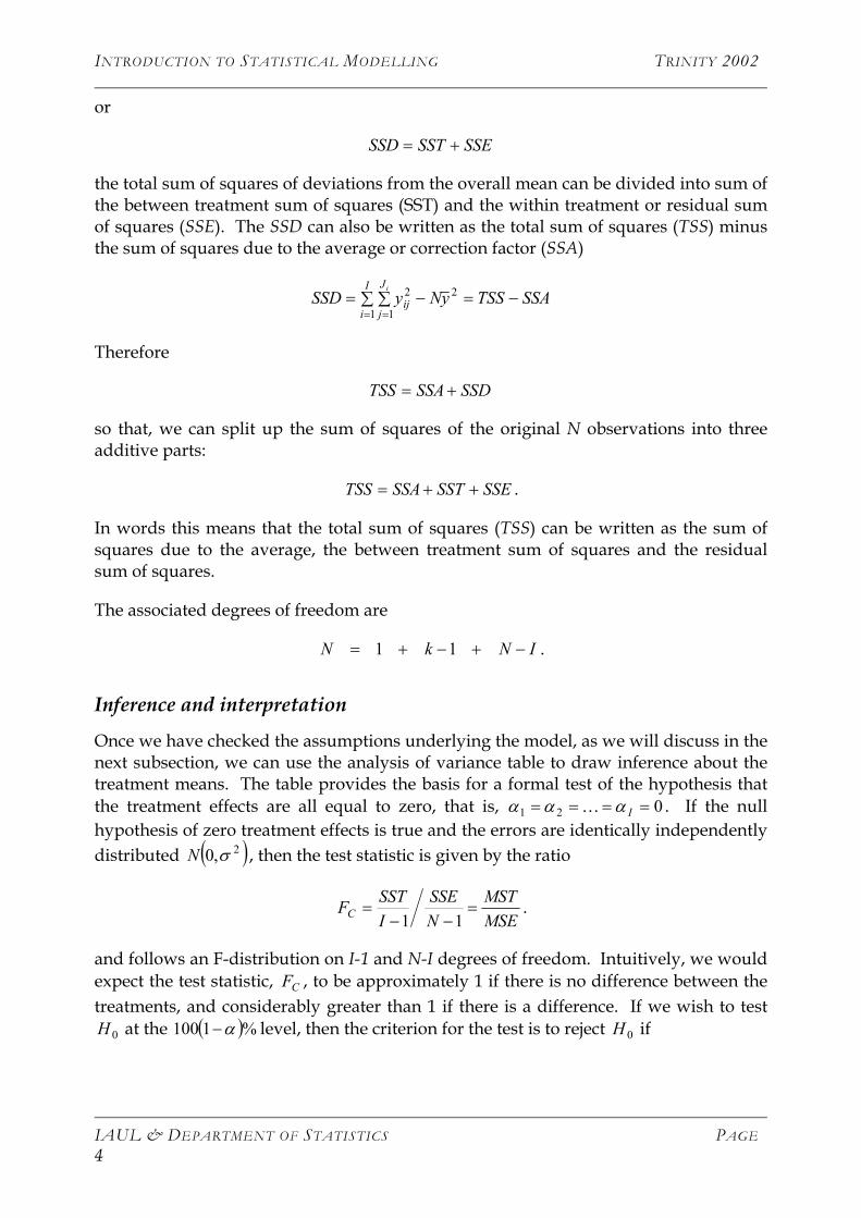
Inference and interpretation

Once we have checked the assumptions underlying the model, as we will discuss in the next subsection, we can use the analysis of variance table to draw inference about the treatment means. The table provides the basis for a formal test of the hypothesis that the treatment effects are all equal to zero, that is, . If the null hypothesis of zero treatment effects is true and the errors are identically independently distributed

021 ==== Iααα K

( )2,0 σN , then the test statistic is given by the ratio

MSEMST

NSSE

ISSTFC =

−−=

11.

and follows an F-distribution on I-1 and N-I degrees of freedom. Intuitively, we would expect the test statistic, , to be approximately 1 if there is no difference between the treatments, and considerably greater than 1 if there is a difference. If we wish to test

at the 100 level, then the criterion for the test is to reject if

CF

0H ( )%1 α− 0H



INIC FF −−−> ,1,1 α ,

where is the100 percentile of a F-distribution with I-1 and N-I degrees of freedom. Its value can be obtained from standard tables or from a software package. Software packages usually provide an exact p-value for the test.

INIF −− ,1,α ( α−1 )

Diagnostic checking of the model

It is important that we check the assumptions underlying our model, namely, errors that are independent and identically normally distributed with constant variance. In order to investigate the validity of these assumptions there are a few standard plots of the residuals that can be used to evaluate their distribution and to check for systematic patterns in the residuals. When the assumptions concerning the adequacy of the model are true, we expect the residuals to vary randomly. Recall from Lecture 2 that the residuals are simply the differences between the observed and fitted values, . Below we consider a few useful plots to investigate the above properties of the residuals. These particular discrepancies should be looked for as a matter of routine, but the experimenter should also be on the alert for other abnormalities. Refer to Lecture Notes 3 for a more detailed discussion.

ijij yy ˆ−

Normal probability plot of the residuals The first plot that we consider for use in checking whether we have satisfied the assumptions is something called a normal probability plot or a quantile-normal plot of the residuals. This plot was introduced in Lecture 3. This plot is used to check the normality assumption since it allows us to investigate whether the residuals are normally distributed: since the residuals can be thought of as estimates of the errors, evidence that the residuals are non-normal might lead us to suspect that the errors are not normal. The interpretation of this plot was discussed in Lecture 3.

Scatterplot of residuals versus predicted values The variability of the residuals should be unrelated to the levels of the response, as we assumed constant variance for the residuals. This can be investigated by plotting the residuals, , against the fitted values, . Sometimes the variance increases as the value of the response increases, which is indicative of non-constant variance.

ijij yy ˆ− ijy

Plot of the residuals in time sequence Sometimes an experimental factor may drift or the skill of the experimenter may improve as the experiment proceeds. Tendencies of this kind may be uncovered by plotting the residuals against time order where it is appropriate.

Example



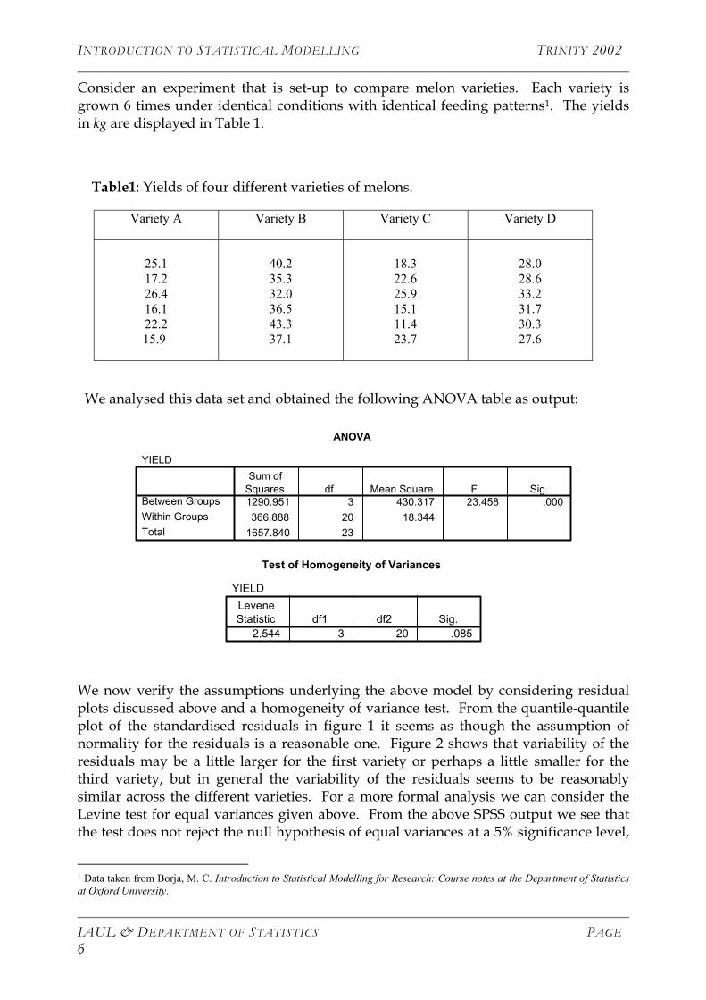
Consider an experiment that is set-up to compare melon varieties. Each variety is grown 6 times under identical conditions with identical feeding patterns1. The yields in kg are displayed in Table 1.

Table1: Yields of four different varieties of melons.

Variety A Variety B Variety C Variety D

25.1 17.2 26.4 16.1 22.2

15.9

40.2 35.3 32.0 36.5 43.3 37.1

18.3 22.6 25.9 15.1 11.4 23.7

28.0 28.6 33.2 31.7 30.3 27.6

We analysed this data set and obtained the following ANOVA table as output:

ANOVA

YIELD

1290.951 3 430.317 23.458 .000366.888 20 18.344

1657.840 23

Between GroupsWithin GroupsTotal

Sum ofSquares df Mean Square F Sig.

Test of Homogeneity of Variances

YIELD

2.544 3 20 .085

LeveneStatistic df1 df2 Sig.

We now verify the assumptions underlying the above model by considering residual plots discussed above and a homogeneity of variance test. From the quantile-quantile plot of the standardised residuals in figure 1 it seems as though the assumption of normality for the residuals is a reasonable one. Figure 2 shows that variability of the residuals may be a little larger for the first variety or perhaps a little smaller for the third variety, but in general the variability of the residuals seems to be reasonably similar across the different varieties. For a more formal analysis we can consider the Levine test for equal variances given above. From the above SPSS output we see that the test does not reject the null hypothesis of equal variances at a 5% significance level,

1 Data taken from Borja, M. C. Introduction to Statistical Modelling for Research: Course notes at the Department of Statistics at Oxford University.



but it does reject it at a 10% level. Thus, it seems that the variability of the residuals is somewhat different for the different varieties, but that the difference is not significant at a 5% level.

In this example, the result of the hypothesis test is highly significant, as indicated by the very small p-value. Thus, the null hypothesis that the yields of all varieties are zero will be rejected in favour of the alternative that at least one variety has a non-zero effect.

Quantiles of Standard Normal

Stan

dard

ised

resi

dual

s

-2 -1 0 1 2

-8-6

-4-2

02

46

Figure 1: QQ-plot for the standardised residuals of the melon yield example.



Fitted : Variety

Res

idua

ls

20 25 30 35

-8-6

-4-2

02

46 3

15

17

Figure 2: Residuals plotted against the fitted values of the expected response.

Treatment contrasts and multiple comparisons

The analysis of variance test above involves only one hypothesis, namely, that of equal treatment means (or treatment effects ). If the hypothesis is rejected in an actual application of the F-test for the equality of means in the one-way layout, the resulting conclusion that the means are not all equal would by itself usually be insufficient to satisfy the experimenter. Methods of making further inferences about the mean are then desirable. In more complicated situations than the one-way ANOVA, the analysis of variance table becomes a very useful tool for identifying aspects of a complicated problem that deserve more attention. It also introduces the SST as a measure of treatment differences. The SST can be broken into components corresponding to the sums of squares for individual orthogonal contrasts. These components of the SST can then be used to explain the differences in the means.

iµ iα

Iµµµ ,,, 21 K

A contrast among the parameters is a linear function of the , , with known contrast coefficients, , subject to the condition ∑ . Furthermore, two contrasts are defined as orthogonal if

Iµµµ ,,, 21 K

iλiµ ∑ =

Ii ii1 µλ

01 ==Ii iλ

01

21 =∑=

I

i i

ii

Nλλ .

Contrasts are only of interest when they define interesting functions of the s. There are many ways to choose contrasts and these depend on the question the researcher is interested in answering. Treatment contrasts are commonly used contrast to compare all of the treatments to a control. Other commonly used contrasts are polynomial

iµ



contrasts and Helmert contrasts. The choice of contrasts can be a rather technical subject and so we will not go into too much detail.

As an example, consider a one-way ANOVA set-up where there are five different diets A, B, C, D and E. Suppose that A is an existing standard diet that serves as the control and that B, C, D and E are new diets. An example of an interesting contrast may be to compare the control diet, A, with the four new diets. This means that we are interested in comparing the control to the average of the other four diets. This contrast would then be

4EDCB

Aµµµµ

µ−−−

−

and by multiplying the contrast by four gives the equivalent contrast

EDCBA µµµµµ −−−−4 .

Software packages such as SPSS accommodate commonly used contrasts such as polynomial contrasts and also allow the user to specify any a priori contrast that may be of interest. Ultimately the choice of which comparison to make is up to the researcher.

One very important final remark we will make involves the issue of multiple comparisons. The specification several different contrasts leads to multiple hypothesis tests that are performed using the same data set. This means that we have to remember to adjust the significance level of any multiple hypothesis tests that we conduct to ensure that the overall level of significance for carrying out all of the tests is equal to the desired level of significance. Recall that the reason for this is that the probability of making at least one type I error is greater than the original significance level when we conduct multiple tests using the same data. There are a number of different significance correction methods described in the literature. Five of the most common ones include adjustments suggested by Bonferroni, Scheffe, Dunnett, Tukey and Sidak. The advantages and disadvantages of using different methods are quite complex and it is common practice to use all of the available methods and then report the most conservative one. Bonferroni’s method is perhaps the simplest and most widely used method. We have discussed this method in the Descriptive Statistics Course.

Non-parametric one-way ANOVA

As was the case in the discussion for linear models, transformations of the response variable can be useful tools for dealing with the problems of heteroscedasticity and non-normality. However, sometimes a transformation cannot solve the problem, in cases like these we can proceed by using a non-parametric test. In the case of two samples, the Mann-Whitney U statistic is the non-parametric equivalent of the two-sample t-test, and in the case of more than two samples, the Kruskal-Wallis test is the non-parametric equivalent of the one-way ANOVA. This approach can be applied when the assumption of normality or equal variance does not hold.



The intuitive idea for the Kruskal-Wallis test is that if you rank all of the data and sum the ranks in each group, then if the groups have no real differences, the sum of the ranks should be the same in each group. If there were differences between the groups, then you would expect the sum of the ranks within each group to be different.

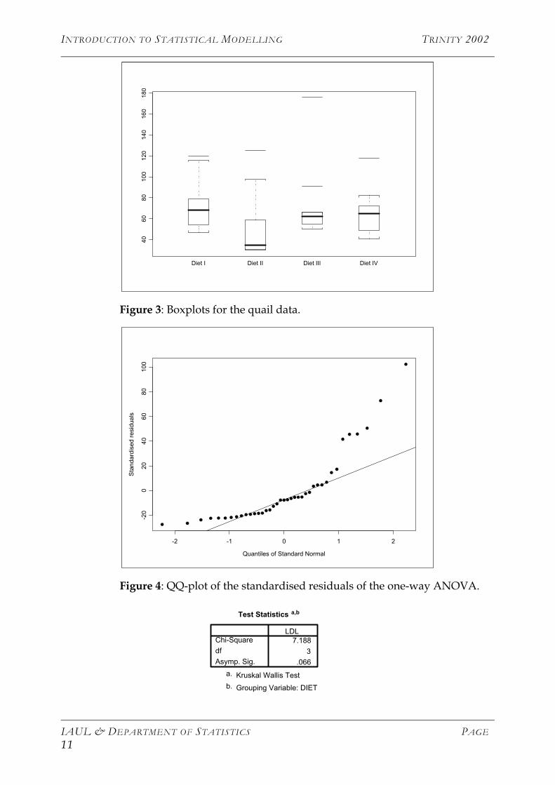
As an example, consider the following experiment investigating LDL cholesterol in quails2. Thirty-nine quails were randomly assigned to four diets, each diet containing a different drug compound, which would hopefully reduce LDL cholesterol. The drug compounds are labelled I, II, III and IV. At the end of the experimental time the LDL cholesterol of each quail was measured. Thus, there are two values relating to each quail, one recording the diet and one indicating the LDL cholesterol level. The data are displayed in Table 2.

Table 2: LDL cholesterol levels in quails exposed to four different diets.

Drug I Drug II Drug III Drug IV

52 67 54 69 116 79 68 47 120 73

36 34 47 125 30 31 30 59 33 98

52 55 66 50 58 176 91 66 61 63

62 71 41 118 48 82 65 72 49

The main interest is to see if whether or not diet has any effect on the mean value of LDL cholesterol level. If we consider the boxplots in figure 3 of the LDL level for each diet, there appear to be significant differences between the diets. We start of by fitting the usual two-way ANOVA model to the data. It is clear from the normal Q-Q plot of the standardised residuals in figure 4 that the residuals do not satisfy the assumption of normality. Any inferences drawn from the results of this ANOVA model will not be valid. Consequently, we perform the Kruskal-Wallis test. The results from this procedure are also presented below.

2 Data taken from Hettmansperger, T. P. and McKean, J. W. (1998). Robust Nonparametric Statistical Methods: Kendall’s Library of Statistics 5. London: Arnold.



4060

8010

012

014

016

018

0

Diet I Diet II Diet III Diet IV

Figure 3: Boxplots for the quail data.


Stan

dard

ised

resi

dual

s

-2 -1 0 1 2

-20

020

4060

8010

0

Figure 4: QQ-plot of the standardised residuals of the one-way ANOVA.

Test Statistics a,b

7.1883

.066

Chi-SquaredfAsymp. Sig.

LDL

Kruskal Wallis Testa.

Grouping Variable: DIETb.



The p-value of 0.066 for Kruskal-Wallis test, although not significant at a 5% level, indicates some difference between the diets as suggested by the diets. A standard one-way ANOVA gives a p-value of 0.35 for the F-test of equal treatment effects. This does not agree with the boxplots in figure 3. The reason for this is that the long right tail of the errors shown in figure 4 adversely affects the test statistic. Unfortunately, there is no easy extension to the problem of multiple comparisons that we will introduce in more details in a later section.

Complete randomised blocks

Introduction

In this section we extend the ideas of the previous section by comparing more than two treatments, using randomised designs with larger block sizes. In blocked designs there are two kinds of effects of interest. The first is the treatment effects, which are of primary interest to the experimenter. The second is the blocks, whose contribution must be accounted for. In practice, blocks might be, for example, different litters of animals, blends of chemical material, strips of land, or contiguous periods of time. In the next section we will consider a replicated factorial design in which the main effects of two factors and the interaction are all of equal interest.

Randomised complete block designs: (1) identify blocks of homogeneous experimental material (units) and (2) randomly assign each treatment to an experimental unit within each block. The blocks are complete in the sense that each block contains all of the treatments. Random assignment of treatments to experimental units allows us to infer causation from a designed experiment. If treatments are randomly assigned to experimental units, then the only systematic differences between the units are the treatments. In observational studies where the treatments are not randomly assigned it is much more difficult to infer causation. So the advantage of this procedure is that treatment comparisons are subject only to the variability within blocks. Block to block variation is eliminated in the analysis. In a completely randomised design applied to the same experimental material, the treatment comparisons would be subject to both within block and between block variability.

Let us consider an example. We consider a randomised block experiment in which a process for the manufacture of penicillin was being investigated, and yield was the response of primary interest3. There were 4 treatments to be studied, denoted by A, B, C and D. It was known that an important raw material, corn steep liquor, was quite variable. Fortunately sufficient blends could be made to allow researchers to run all 4 treatments within each of 5 blocks (blends of corn steep liquor). Furthermore, the experiment was protected against extraneous unknown sources of bias by running the

3 Example taken from Box, Hunter and Hunter. 1978. Statistics for Experimenters: An Introduction to Design, Data Analysis and Model Building. John Wiley, New York.



treatments in random order within each block. The randomised block design is given in Table 3.

Table 3: Randomised block design on penicillin manufacture4

Treatment

Block A B C D

Blend 1

Blend 2

Blend 3

Blend 4

Blend 5

89(1)

84(4)

81(2)

87(1)

79(3)

88(3)

77(2)

87(1)

92(3)

81(4)

97(2)

92(3)

87(4)

89(2)

80(1)

94(4)

79(1)

85(3)

84(4)

88(2)

The model and assumptions

The model for a randomised complete block design is given by

( )2,0 i.i.d. ,,,1;,,1, σεεβαµ NJjIiy ijijjiij KK ==+++= .

There are J blocks with I treatments observed within each block. As before the parameter is viewed as a grand mean, is an unknown fixed effect for the ith treatment, and is an unknown fixed effect for the jth block. The theoretical basis for the analysis of this model is precisely as in the balanced one-way ANOVA. As before the computations can be summarised in an ANOVA table, as we will show in the following section.

µ iα

jβ

ANOVA table As was the case for the one-way layout, the results of fitting model the model for a complete randomised block design are typically represented in an ANOVA table, which is a summary of the modelling procedure and can be calculated using most statistical software packages. As we are interested in the interpretation rather than theory, we only consider an example of what an ANOVA table looks like for a complete block design, thereby avoiding unnecessary mathematics.

Table 4: ANOVA table for a complete randomised block design

4 The superscripts in parentheses associated with the observations indicate the random order in which the experiments were run within each blend.




Intercept 1 SSA MSA

Treatments I-1 SST MST MST/MSE

Blocks J-1 SSB MSB MSB/MSE

Residuals (I-1)(J-1) SSE MSE

Total IJ TSS

In the table above SSA, SST, SSE, TSS, MST and MSE are simply summaries calculated from the observed data, similar to what we saw for the one-way ANOVA table. Furthermore, I is the number of treatments and J is the number of blocks. The two test statistics are produced in a similar way to the one-way case. We will consider the two hypotheses involved in a little more detail in the following section.


Table 4 provides the basis for a formal test of the hypothesis that the treatment effects are all equal to zero, as well as a formal test for the hypothesis that the block effects are all equal to zero. The F-statistic, MSEMSTFT = , is used to test whether there are significant treatment effects, i.e., it is used to test

0:0: 210

≠====

iA

I

HH

αααα

one least at K

.

The statistic follows an F-distribution on I-1 and (I-1)(J-1) degrees of freedom. If we wish to test at the 100 level, then the criterion for the test is to reject if 0H ( )%1 α− 0H

( )( 11,1,1 −−−−> JIIT FF α )

) )

.

( )( 11,1, −−− JIIFα is the100 percentile of a F-distribution with I-1 and (I-1)(J-1) degrees of freedom and its value can be obtained from standard tables or from a software package.

( α−1

Similarly, the F-statistic, MSEMSBFB = , is used to test whether there are significant block effects, i.e., it is used to test



0:0: 210

≠====

jA

J

HH

ββββ

one least at K

.

The F-statistic provides a test of whether we can isolate comparative differences in the block effects. Thus, a significant test indicates that blocking was a worthwhile exercise. If we wish to test at the 100 level, then the criterion for the test is to reject

if 0H ( )%1 α−

0H

( )( 11,1,1 −−−−> JIJT FF α )

) )

.

( )( 11,1, −−− JIJFα is the100 percentile of a F-distribution with J-1 and (I-1)(J-1) degrees of freedom.

( α−1

Diagnostic checking of the model

The assumptions underlying the randomised complete block design model are similar to those of the one-way ANOVA model. These assumptions need to be verified in order for the model to be valid. We can use the same methods as for the one-way ANOVA model to achieve this.

Example

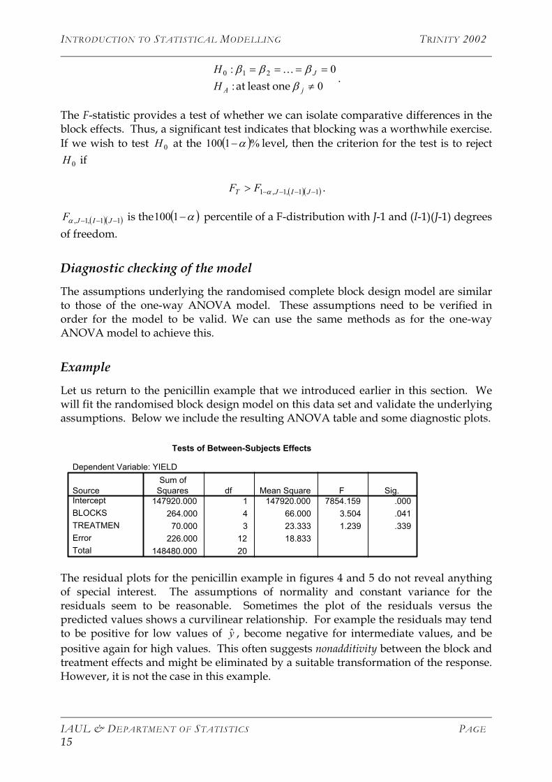
Let us return to the penicillin example that we introduced earlier in this section. We will fit the randomised block design model on this data set and validate the underlying assumptions. Below we include the resulting ANOVA table and some diagnostic plots.

Tests of Between-Subjects Effects

Dependent Variable: YIELD

147920.000 1 147920.000 7854.159 .000264.000 4 66.000 3.504 .04170.000 3 23.333 1.239 .339

226.000 12 18.833148480.000 20

SourceInterceptBLOCKSTREATMENErrorTotal


The residual plots for the penicillin example in figures 4 and 5 do not reveal anything of special interest. The assumptions of normality and constant variance for the residuals seem to be reasonable. Sometimes the plot of the residuals versus the predicted values shows a curvilinear relationship. For example the residuals may tend to be positive for low values of , become negative for intermediate values, and be positive again for high values. This often suggests nonadditivity between the block and treatment effects and might be eliminated by a suitable transformation of the response. However, it is not the case in this example.

y



Fitted : 1 + TREATMEN + BLOCKS

Res

idua

ls

80 85 90 95

-4-2

02

46

15

1220

Figure 5: Residuals versus fitted values for penicillin example.


-2 -1 0 1 2

-4-2

02

46

Figure 6: Q-Q plot of the standardised residuals in the penicillin example. The p-value of 0.339 for the hypothesis of zero treatment effects, suggests that the four different treatments have not resulted in different yields. The variability among the treatment averages can be reasonably attributed to experimental error. We reject the null hypothesis of no blend-to-blend variation, as suggested by the small p-value (0.041), thus there are significant block effects.



The two-way factorial design

Introduction

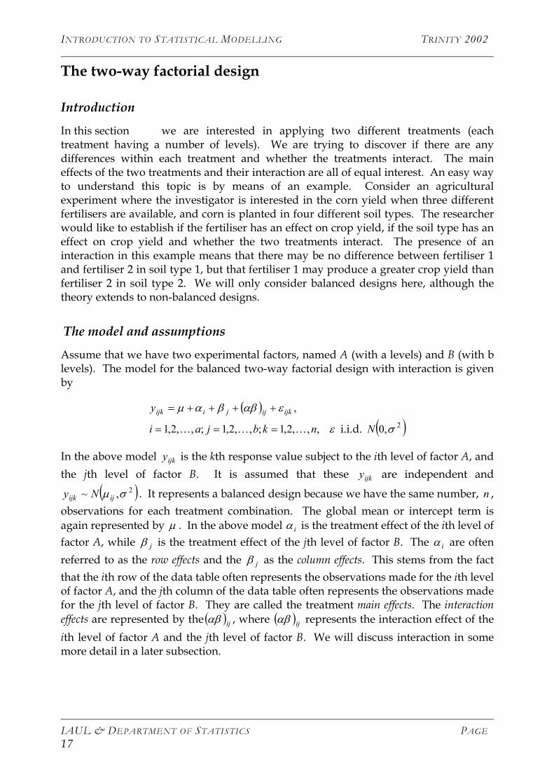
In this section we are interested in applying two different treatments (each treatment having a number of levels). We are trying to discover if there are any differences within each treatment and whether the treatments interact. The main effects of the two treatments and their interaction are all of equal interest. An easy way to understand this topic is by means of an example. Consider an agricultural experiment where the investigator is interested in the corn yield when three different fertilisers are available, and corn is planted in four different soil types. The researcher would like to establish if the fertiliser has an effect on crop yield, if the soil type has an effect on crop yield and whether the two treatments interact. The presence of an interaction in this example means that there may be no difference between fertiliser 1 and fertiliser 2 in soil type 1, but that fertiliser 1 may produce a greater crop yield than fertiliser 2 in soil type 2. We will only consider balanced designs here, although the theory extends to non-balanced designs.

The model and assumptions

Assume that we have two experimental factors, named A (with a levels) and B (with b levels). The model for the balanced two-way factorial design with interaction is given by

( )( )2,0,,,2,1;,,2,1;,,2,1

,

σε

εαββαµ

Nnkbjai

y ijkijjiijk

i.i.d. KKK ===

++++=

In the above model is the kth response value subject to the ith level of factor A, and the jth level of factor B. It is assumed that these are independent and

ijky

ijky

( )2,~ σµ ijijk Ny . It represents a balanced design because we have the same number, n , observations for each treatment combination. The global mean or intercept term is again represented by . In the above model is the treatment effect of the ith level of factor A, while is the treatment effect of the jth level of factor B. The are often referred to as the row effects and the as the column effects. This stems from the fact that the ith row of the data table often represents the observations made for the ith level of factor A, and the jth column of the data table often represents the observations made for the jth level of factor B. They are called the treatment main effects. The interaction effects are represented by the , where ( represents the interaction effect of the ith level of factor A and the jth level of factor B. We will discuss interaction in some more detail in a later subsection.

µ iα

ijαβ

jβ iα

jβ

( )ijαβ )



ANOVA table Again we consider the ANOVA table for the above model by avoiding unnecessary mathematical detail. The general form of the ANOVA table is presented in table 5.

Table 5: ANOVA table for a balanced two-way factorial design with interaction


Intercept 1 SSInt MSInt

Factor A a-1 SSA MSA MSA/MSE

Factor B b-1 SSB MSB MSB/MSE

Interaction (a-1)(b-1) SS(AB) MS(AB) MS(AB)/MSE

Error ab(n-1) SSE MSE

Total TSS

As before the quantities in the table above are simply summaries calculated from the observed data, similar to what we saw for the one-way ANOVA table and the block design. The three test statistics are produced in a similar way than before, and is based on the same intuitive approach. That is, we are considering estimating how much of the overall variation each factor and the interaction explain, compared to the residual (error) variation. The next subsection will look at the relevant hypotheses in some more detail.


Again the ANOVA table provides the basis for formal tests of all the relevant hypotheses that we may be interested in. There are three main hypothesis tests of interest here, namely, the test for significant treatment effects for factor A, the test for significant treatment effects for factor B and the test for significant interaction effects. As with the previous sections, to test each of the hypotheses, we compare the test statistic given in the last column with the F-distribution with appropriate degrees of freedom. The appropriate degrees of freedom are the degrees of freedom associated with the source of variation and the degrees of freedom associated with the error.



The F-statistic, MSEMSAFA = , is used to test whether there are significant treatment effects for factor A, i.e.

0:0: 210

≠====

iA

a

HH

αααα

one least at K

.

Similar to the one-way ANOVA the statistic follows an F-distribution on a-1 and (a-1)(b-1) degrees of freedom. If we wish to test at the 100 level, then the criterion for the test is to reject if

0H ( )%1 α−

0H

( )( 11,1,1 −−−−> baaA FF α )

) )

where is the100 percentile of a F-distribution with a-1 and (a-1)(b-1) degrees of freedom.

( )( 11,1,1 −−−− baaF α ( α−1

Similarly, the F-statistic, MSEMSBFB = , is used to test whether there are significant treatment effects for factor B, i.e.

0:0: 210

≠====

jA

b

HH

ββββ

one least at K

.

If we wish to test at the 100 level, then the criterion for the test is to reject if

0H ( )%1 α−

0H

( )( 11,1,1 −−−−> babB FF α )

) )

where is the100 percentile of a F-distribution with b-1 and (a-1)(b-1) degrees of freedom.

( )( 11,1,1 −−−− babF α ( α−1

The third hypothesis that we want to test is that of no significant interaction effects. The F-statistic, ( ) MSEABMSFAB = , provides us with the basis of doing that. The corresponding hypothesis can be formulated as

0:

,,,2,1;,,2,1,0:0

≠

===

ijA

ij

H

bjaiH

αβ

αβ

one least at KK

When we test the null hypothesis of no interaction at the 100 level, the criterion for the test is to reject if

( )%1 α−

0H

( ) ( )( 11,1,1 −−−−> banabAB FF α )



where ) is the100 percentile of a F-distribution with ab(n-1) and (a-1)(b-1) degrees of freedom. Normally all these values are provided by the software package and thus there is no need to calculate them yourself.

( ) ( )( 11,1,1 −−−− banabF α ( α−1 )

Example

Our example involves an experiment in which haemoglobin levels in the blood of brown trout were measured after treatment with four rates of sulfamerazine. Two methods of administering the sulfamerazine were used. Ten fish were measured for each rate and each method. The data are given in Table 65.

Table 6: Data for the haemoglobin example.

Rate

Method 1 2 3 4

A

6.7 7.8 5.5 8.4 7.0 7.8 8.6 7.4 5.8 7.0

9.9 8.4

10.4 9.3

10.7 11.9 7.1 6.4 8.6

10.6

10.4 8.1

10.6 8.7

10.7 9.1 8.8 8.1 7.8 8.0

9.3 9.3 7.2 7.8 9.3

10.2 8.7 8.6 9.3 7.2

B

7.0 7.8 6.8 7.0 7.5 6.5 5.8 7.1 6.5 5.5

9.9 9.6

10.2 10.4 11.3 9.1 9.0

10.6 11.7 9.6

9.9 9.6

10.2 10.4 11.3 10.9 8.0

10.2 6.1

10.7

11.0 9.3

11.0 9.0 8.4 8.4 6.8 7.2 8.1

11.0

If we now fit a two-way ANOVA to the data we obtain the following results:

5 This data is taken from Rencher, A. C. (2000). Linear Models in Statistics. Wiley: New York.



ANOVA output

Dependent Variable: HEMOGLOB

6102.271 1 6102.271 3956.626 .00090.304 3 30.101 19.517 .0002.346 1 2.346 1.521 .2214.803 3 1.601 1.038 .381

111.045 72 1.5426310.770 80

SourceInterceptRATEMETHODRATE * METHODErrorTotal


The approach is generally to first test the hypothesis that there is an interaction, since the significance of the main effects cannot be tested in the presence of an interaction. If there is a significant interaction we can use something called an interaction plot to allow us to examine the interaction and explain what is happening. If there is no interaction we then consider testing for the effects of the two treatments.

In the above example the interaction term is not significant. If we just consider the effect of method on its own, it appears to be strongly insignificant, whereas the effect of rate on its own is very significant. The underlying normality and constant variance assumption have to be verified in order for the ANOVA results to be valid. This has been done for this example, but the results are not reported here.

Interactions

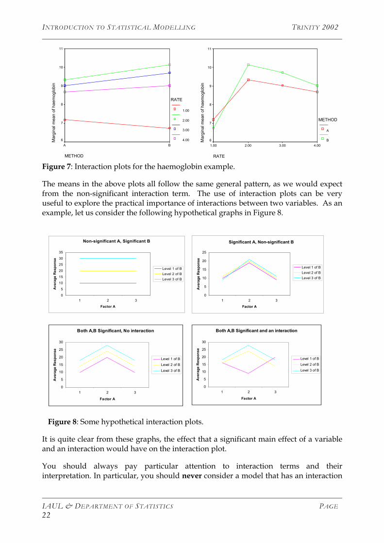
Although the interaction term is not significant in the above example, we present two interaction plots from the example to illustrate how interaction affects can be graphically represented. An interaction plot basically plots the mean of each level of one treatment variable, at each level of the other treatment variable. If all the means follow the same general pattern, then there will be no interaction. If some levels follow different patterns, there will be an interaction. In the haemoglobin example we get the two plots in Figure 7.



METHOD

BA

Mar

gina

l mea

n of

hae

mog

lobi

n11

10

9

8

7

6

RATE

1.00

2.00

3.00

4.00

RATE

4.003.002.001.00

Mar

gina

l mea

n of

hae

mog

lobi

n

11

10

9

8

7

6

METHOD

A

B

Figure 7: Interaction plots for the haemoglobin example.

The means in the above plots all follow the same general pattern, as we would expect from the non-significant interaction term. The use of interaction plots can be very useful to explore the practical importance of interactions between two variables. As an example, let us consider the following hypothetical graphs in Figure 8.

Significant A, Non-significant B

0

5

10

15

20

25

1 2 3

Factor A

Ave

rage

Res

pons

e

Level 1 of BLevel 2 of BLevel 3 of B

Non-significant A, Significant B

0

5

10

15

20

25

30

35

1 2 3

Factor A

Ave

rage

Res

pons

e


Both A,B Significant, No interaction

0

5

10

15

20

25

30

1 2 3

Factor A

Ave

rage

Res

pons

e


Both A,B Significant and an interaction

0

5

10

15

20

25

30

1 2 3

Factor A

Ave

rage

Res

pons

e


Figure 8: Some hypothetical interaction plots.

It is quite clear from these graphs, the effect that a significant main effect of a variable and an interaction would have on the interaction plot.

You should always pay particular attention to interaction terms and their interpretation. In particular, you should never consider a model that has an interaction



between two variables without having both of the variables included; not including the main effects of an interaction does not make intuitive sense and is dangerous, although a lot of software packages will allow you to do this. You should also be careful when interpreting the results of any particular modelling procedure, if you have a significant interaction between two variables, you can not say anything about the effect of one variable on the response, however, you can say that your variable of interest and its interaction with another variable has an effect on the response. In many observational studies, interactions can often be one of the most interesting findings, since they imply that the two variables do not act in isolation on the response, they in fact act together and this joint interaction can give a researcher great insight into the effect of the variables on the response.

Treatment contrasts and multiple comparisons

As an example consider a two-factor study where the response is the score on a 20 item multiple choice test over a taped lecture, and the two factors are cognitive style (FI=Field Independent, FD=Field Dependent) and study technique (NN=No notes, SN=Student Notes, PO=Partial Outline Supplied, CO=Complete Outline)6.

We initially consider an interaction plot for this data to see whether there is any evidence that there may be an interaction.

cogstyle

mea

n of

sco

re

1314

1516

1718

FD FI

studytec

SNCOPONN

It appears from the above plot that there is an interaction between cognitive style and study technique, so we consider the ANOVA with the interaction term included. The ANOVA table is as follows:

6 The data were collected by Frank (1984) “Effects of field independence-dependence and study technique on learning from a lecture” Amer.Educ.Res.J., 21, 669-678



ANOVA output

Dependent Variable: SCORE

25.010 1 25.010 7.784 .006320.183 3 106.728 33.216 .00027.260 3 9.087 2.828 .043

308.462 96 3.213

SourceCOGSTYLESTUDYTECCOGSTYLE * STUDYTECError


Clearly from this table, the interaction term is significant. It is now of interest to perform an analysis of effects. In this example we are interested in testing for differences in each of the four study techniques. However, as these techniques occur in each of the two cognitive style groups we will have to carry out the multiple comparisons in each group. The results from this analysis are given below. The interesting result from this analysis is that it appears that the differences in study technique are the same in each of the cognitive method groups; thus suggesting that most of the differences in the response variables come from differences in study technique rather than cognitive style.

95 % simultaneous confidence intervals for specified linear combinations, by the Sidak method critical point: 2.9238 response variable: cogstyle intervals excluding 0 are flagged by '****' Estimate Std.Error Lower Bound Upper Bound CO.adj1-NN.adj1 4.4600 0.703 2.4100 6.520 **** CO.adj1-PO.adj1 0.7690 0.703 -1.2900 2.820 CO.adj1-SN.adj1 2.1500 0.703 0.0982 4.210 **** NN.adj1-PO.adj1 -3.6900 0.703 -5.7500 -1.640 **** NN.adj1-SN.adj1 -2.3100 0.703 -4.3600 -0.252 **** PO.adj1-SN.adj1 1.3800 0.703 -0.6710 3.440 CO.adj2-NN.adj2 4.3800 0.703 2.3300 6.440 **** CO.adj2-PO.adj2 0.0769 0.703 -1.9800 2.130 CO.adj2-SN.adj2 -0.3850 0.703 -2.4400 1.670 NN.adj2-PO.adj2 -4.3100 0.703 -6.3600 -2.250 **** NN.adj2-SN.adj2 -4.7700 0.703 -6.8200 -2.710 **** PO.adj2-SN.adj2 -0.4620 0.703 -2.5200 1.590

The confidence intervals above are represented graphically in figure 8 below.



( (

( (

( (

( (

( (

( (

) )

) )

) )

) )

) )

) )

CO.adj1-NN.adj1 CO.adj1-PO.adj1 CO.adj1-SN.adj1 NN.adj1-PO.adj1 NN.adj1-SN.adj1 PO.adj1-SN.adj1 CO.adj2-NN.adj2 CO.adj2-PO.adj2 CO.adj2-SN.adj2 NN.adj2-PO.adj2 NN.adj2-SN.adj2 PO.adj2-SN.adj2

-7 -6 -5 -4 -3 -2 -1 0 1 2 3 4 5 6 7 simultaneous 95 % confidence limits, Sidak method

response variable: cogstyle

Figure 8: Graphical representation of confidence intervals above.

Non-parametric two-way ANOVA

Just as in the one-way case, we can equivalently consider a non-parametric two-way ANOVA. However, it now becomes considerably more complex and the common test statistic in this setting is restricted to the following special case. Consider the case where you have two factors, one representing the treatment of interest and the other representing a “blocking” variable (see the section on complete block designs). The interest is then in assessing whether there are any differences between the treatments and to do this we can use the Friedman rank sum test. The generalisation to more complex settings is possible but requires a lot of work and is not generally implemented in the computing packages. The interpretation is identical to that of the Kruskal-Wallis test for the one-way ANOVA, you will get a test statistic and also a p-value, and as usual you can conclude that there is a significant difference between your treatments if the p-value is less than 0.05.

More than two factors and covariates

Although all of the techniques described above only cover the case of either one or two-factor models the same ideas can be extended to three- or more factor models or to models that include continuous covariates. The main issue to consider is which model you are going to fit – i.e. do you fit the full factorial model which includes all the main effects and all of the interactions (two-way and higher) or do you only fit a subset of this model, perhaps one which only contains the main effects and two-factor interactions. These decisions will be guided by the aim of your analysis and what hypothesis you wish to test and is called model selection. You have the same choices if you include covariates in the model. In the next section we will consider the case where model includes continuous covariates. This type of analysis is called analysis of covariance.



Analysis of covariance

Introduction

Analysis of covariance incorporates one or more regression variables into an analysis of variance. The regression variables are typically continuous and are referred to as covariates, hence the name analysis of covariance. In this course we will only examine the use of a single covariate. We discuss the analysis of covariance at the hand of an example that involves one-way analysis of variance and a covariate.

Example

We consider data on the body weights (in kilograms) and heart weights (in grams) for domestic cats of both sexes that were given digitalis. Part of the original data is presented in Table 7 7, 8. The primary interest is to determine whether females’ heart weights differ from males’ when both have received digitalis. A first step in the analysis might be to fit a one-way ANOVA model by ignoring the body weight variable. Such a model would be given by

,24,,1;2,1 K==++= jiY ijiij εαµ

where the are the heart weights. The ANOVA output for this model is given below. ijy

Table 7: Body weights (kg) and heart weights (g) of domestic cats with digitalis.

7 The data was originally published by Fisher, R. A. (1947). The analysis of covariance method for the relation between a part and the whole. Biometrics, 3, 65-68. 8 The data is taken from Christensen, R. (1996). Analysis of Variance, Design and Regression: Applied statistical methods. New York: Chapman & Hall. Here a subset of the original data is used to illustrate the application of the analysis of covariance.



Females Males

Body Heart Body Heart Body Heart Body Heart

2.3 3.0 2.9 2.4 2.3 2.0 2.2 2.1 2.3 2.1 2.1 2.2

9.6 10.6 9.9 8.7

10.1 7.0

11.0 8.2 9.0 7.3 8.5 9.7

2.0 2.3 2.2 2.3 2.1 2.0 2.9 2.7 2.6 2.3 2.6 2.1

7.4 7.3 7.1 9.0 7.6 9.5

10.1 10.2 10.1 9.5 8.7 7.2

2.8 3.1 3.0 2.7 2.8 2.1 3.3 3.4 2.8 2.7 3.2 3.0

10.0 12.1 13.8 12.0 12.0 10.1 11.5 12.2 13.5 10.4 11.6 10.6

2.9 2.4 2.2 2.9 2.5 3.1 3.0 2.5 3.4 3.0 2.6 2.5

9.4 9.3 7.2

11.3 8.8 9.9

13.3 12.7 14.4 10.0 10.5 8.6

one-way ANOVA output

BRAIN

56.117 1 56.117 23.444 .000110.106 46 2.394166.223 47

Between GroupsWithin GroupsTotal


We see that the effect due to sexes is highly significant in the one-way ANOVA. Until now we have not made use of the extra value of body weight that we have in addition to the brain weight variable. It is natural to consider whether effective use can be made of this value.

In order to make use of the body weight observations, we add a regression term to the one-way ANOVA model above and fit the traditional analysis of covariance model,

( )2,0 i.i.d. ,24,,1;2,1, σεεγαµ Njizy ijijijiij K==+++=

In the above model the ’s are the body weights and is a slope parameter associated with body weights. Note that this model is an extension of the simple linear regression model between the s and s in which we allow a different intercept for each sex. The ANOVA table for this model is given below.

ijz γ

y z iµ



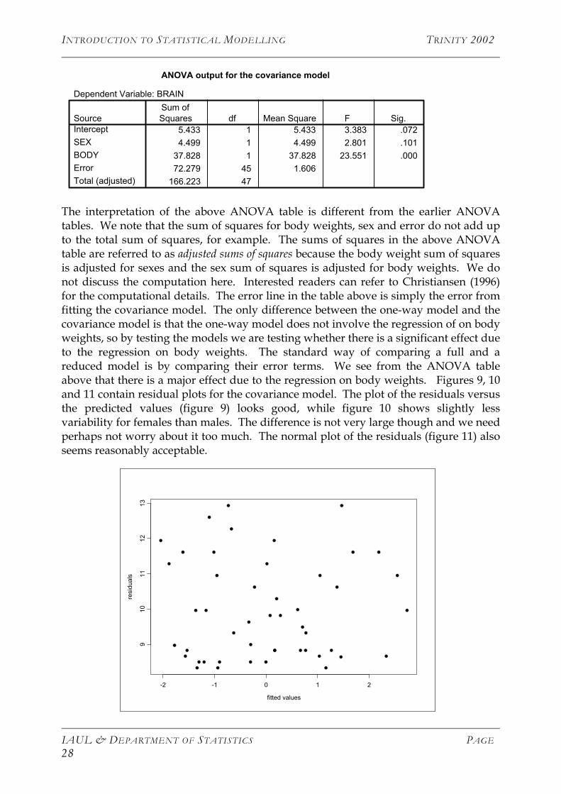
ANOVA output for the covariance model

Dependent Variable: BRAIN

5.433 1 5.433 3.383 .0724.499 1 4.499 2.801 .101

37.828 1 37.828 23.551 .00072.279 45 1.606

166.223 47

SourceInterceptSEXBODYErrorTotal (adjusted)


The interpretation of the above ANOVA table is different from the earlier ANOVA tables. We note that the sum of squares for body weights, sex and error do not add up to the total sum of squares, for example. The sums of squares in the above ANOVA table are referred to as adjusted sums of squares because the body weight sum of squares is adjusted for sexes and the sex sum of squares is adjusted for body weights. We do not discuss the computation here. Interested readers can refer to Christiansen (1996) for the computational details. The error line in the table above is simply the error from fitting the covariance model. The only difference between the one-way model and the covariance model is that the one-way model does not involve the regression of on body weights, so by testing the models we are testing whether there is a significant effect due to the regression on body weights. The standard way of comparing a full and a reduced model is by comparing their error terms. We see from the ANOVA table above that there is a major effect due to the regression on body weights. Figures 9, 10 and 11 contain residual plots for the covariance model. The plot of the residuals versus the predicted values (figure 9) looks good, while figure 10 shows slightly less variability for females than males. The difference is not very large though and we need perhaps not worry about it too much. The normal plot of the residuals (figure 11) also seems reasonably acceptable.

fitted values

resi

dual

s

-2 -1 0 1 2

910

1112

13



Figure 9: Residuals versus predicted values of the covariance model

-2-1

01

2

FEMALE MALE

sex

resi

dual

s

Figure 10: Box plots of residuals by sex for the residuals of the covariance model.


-2 -1 0 1 2

-2-1

01

2

Figure 11: Normal Q-Q plot of the standardised residuals of the covariance model

Analysis of covariance in designed experiments



In the previous example we are dealing with an observational study as opposed to a designed experiment. In a designed experiment the role of covariates is solely to reduce the error of treatment comparisons. For a covariate to be of help in an analysis it must be related to the dependent variable. Unfortunately, improper use of covariates can invalidate, or alter, comparisons among treatments. In the observational study above the very nature of what we were comparing changed when we adjusted for body weights. Originally we investigated whether heart weights were different for females and males. The analysis of covariance examined whether there were differences between female and male heart weights beyond what could be accounted for by the regression on body weights. These are quite different interpretations.

In a designed experiment, we want to investigate the effects of the treatments and not the treatments adjusted for some covariates. Cox (1958) refers to a supplementary observation that may be used to increase precision as a concomitant observation. It is stated that an important condition for the use of a concomitant observation is that after its use, estimated effects for the desired main observation shall still be obtained. This condition means that the concomitant observations should be unaffected by the treatments. In practice this means that either the concomitant observations are taken before the assignment of the treatments, or the concomitant observations are made after the assignment of the treatments, but before the effect of treatments has had time to develop. These requirements on the nature of covariates in a designed experiment are imposed so that the treatment effects do not depend on the presence or absence of the covariates in the analysis. The treatment effects are logically independent regardless of whether covariates are measured or incorporated in the analysis.

Multivariate analysis of variance (MANOVA)

The multivariate approach to analysing data that contain repeated measurements on each subject involves using the repeated measures as separate dependent variables in a collection of standard analyses of variance. The method of analysis, known as multivariate analysis of variance (MANOVA), then combines results from the several ANOVAs. A detailed discussion of MANOVA is beyond the scope of this course. Readers who are interested to learn more about the subject are referred to Johnson and Wichern (1992).

A. Roddam(2000), K. Javaras and W. Vos (2002)

References

Box, G., J. S., Hunter, W. G., Hunter, J. S. (1978). Statistics for Experimenters: an Introduction to design, Data Analysis, and Model Building. New York: John Wiley.

Christensen, R. (1996). Analysis of Variance, Design and Regression: Applied statistical methods. New York: Chapman & Hall.



Cox, D. R. (1958). Planning of Experiments. New York: John Wiley.

Fisher, R. A. (1947). The analysis of covariance method for the relation between a part and the whole. Biometrics, 3, 65-68.

Hettmansperger, T. P. and McKean, J. W. (1998). Robust Nonparametric Statistical Methods: Kendall’s Library of Statistics 5. London: Arnold.

Johnson, R. A. and Wichern, D. W. (1992). Applied Multivariate Statistical Analysis. New York: Prentice Hall.

Rencher, A. C. (2000). Linear Models in Statistics. Wiley: New York.

Scheffé, H. (1959). The Analysis of Variance. New York: John Wiley.


Date post:	18-May-2018
Category:	Documents
Upload:	dangcong
View:	213 times
Download:	0 times

The Analysis of Variance - Department of Statistics, … TO STATISTICAL MODELLING TRINITY 2002 The...

Documents