The ApolloScape Dataset for Autonomous Driving

Xinyu Huang, Xinjing Cheng, Qichuan Geng, Binbin Cao,

Dingfu Zhou, Peng Wang, Yuanqing Lin, and Ruigang Yang

Baidu Research, Beijing, China

National Engineering Laboratory of Deep Learning Technology and Application, China{huangxinyu01,chengxinjing,gengqichuan,caobinbin}@baidu.com{zhoudingfu,wangpeng54,linyuanqing,yangruigang}@baidu.com

Abstract

Scene parsing aims to assign a class (semantic) label

for each pixel in an image. It is a comprehensive anal-

ysis of an image. Given the rise of autonomous driving,

pixel-accurate environmental perception is expected to be a

key enabling technical piece. However, providing a large

scale dataset for the design and evaluation of scene pars-

ing algorithms, in particular for outdoor scenes, has been

difficult. The per-pixel labelling process is prohibitively ex-

pensive, limiting the scale of existing ones. In this paper,

we present a large-scale open dataset, ApolloScape, that

consists of RGB videos and corresponding dense 3D point

clouds. Comparing with existing datasets, our dataset has

the following unique properties. The first is its scale, our

initial release contains over 140K images – each with its

per-pixel semantic mask, up to 1M is scheduled. The second

is its complexity. Captured in various traffic conditions, the

number of moving objects averages from tens to over one

hundred (Figure 1). And the third is the 3D attribute, each

image is tagged with high-accuracy pose information at cm

accuracy and the static background point cloud has mm rel-

ative accuracy. We are able to label these many images by

an interactive and efficient labelling pipeline that utilizes

the high-quality 3D point cloud. Moreover, our dataset also

contains different lane markings based on the lane colors

and styles. We expect our new dataset can deeply bene-

fit various autonomous driving related applications that in-

clude but not limited to 2D/3D scene understanding, local-

ization, transfer learning, and driving simulation.

1. Introduction

Semantic segmentation, or scene parsing, of urban street

views is one of major research topics in the area of au-

tonomous driving. A number of datasets have been col-

lected in various cities in recent years, aiming to increase

Figure 1. An example of color image (top), 2D semantic label

(middle), and depth map for the static background (bottom).

variability and complexity of urban street views. The

Cambridge-driving Labeled Video database (CamVid) [1]

could be the first dataset with semantic annotated videos.

The size of the dataset is relatively small, which contains

701 manually annotated images with 32 semantic classes

captured from a driving vehicle. The KITTI Vision Bench-

mark Suite [4] collected and labeled a dataset for different

computer vision tasks such as stereo, optical flow, 2D/3D

object detection and tracking. For instance, 7,481 training

and 7,518 test images are annotated by 2D and 3D bound-

ing boxes for the tasks of object detection and object orien-

tation estimation. This dataset contains up to 15 cars and

30 pedestrians in each image. However, pixel-level annota-

tions are only made partially by third parties without quality

11067

controls. As a result, semantic segmentation benchmark is

not provided directly. The Cityscapes Dataset [2] focuses

on 2D semantic segmentation of street views that contains

30 classes, 5,000 images with fine annotations, and 20,000

images with coarse annotations. Although video frames are

available, only one image (20th image in each video snip-

pet) is annotated. Similarly, the Mapillary Vistas Dataset [7]

selected and annotated a larger set of images with fine an-

notations, which has 25,000 images with 66 object cate-

gories. The TorontoCity benchmark [13] collects LIDAR

data and images including stereo and panoramas from both

drones and moving vehicles. Currently, this could be the

largest dataset, which covers the greater Toronto area. How-

ever, as mentioned by authors, it is not possible to manually

label this scale of dataset. Therefore, only two semantic

classes, i.e., building footprints and roads, are provided as

the benchmark task of the segmentation.

In this paper, we present an on-going project aimed to

provide an open large-scale comprehensive dataset for ur-

ban street views. The eventual dataset will include RGB

videos with millions high resolution image and per pixel an-

notation, survey-grade dense 3D points with semantic seg-

mentation, stereoscopic video with rare events, night-vision

sensors. Our on-going collection will further cover a wide

range of environment, weather, and traffic conditions. Com-

paring with existing datasets, our dataset has the following

characteristics:

1. The first subset, 143,906 image frames with pixel an-

notations, has been released. We divide our dataset

into easy, moderate, and hard subsets. The difficulty

levels are measured based on number of vehicles and

pedestrians per image that often indicates the scene

complexity. Our goal is to capture and annotate around

one million video frames and corresponding 3D point

clouds.

2. Our dataset has survey-grade dense 3D point cloud for

static objects. A rendered depth map is associated with

each image, creating the first pixel-annotated RGB-D

video for outdoor scenes.

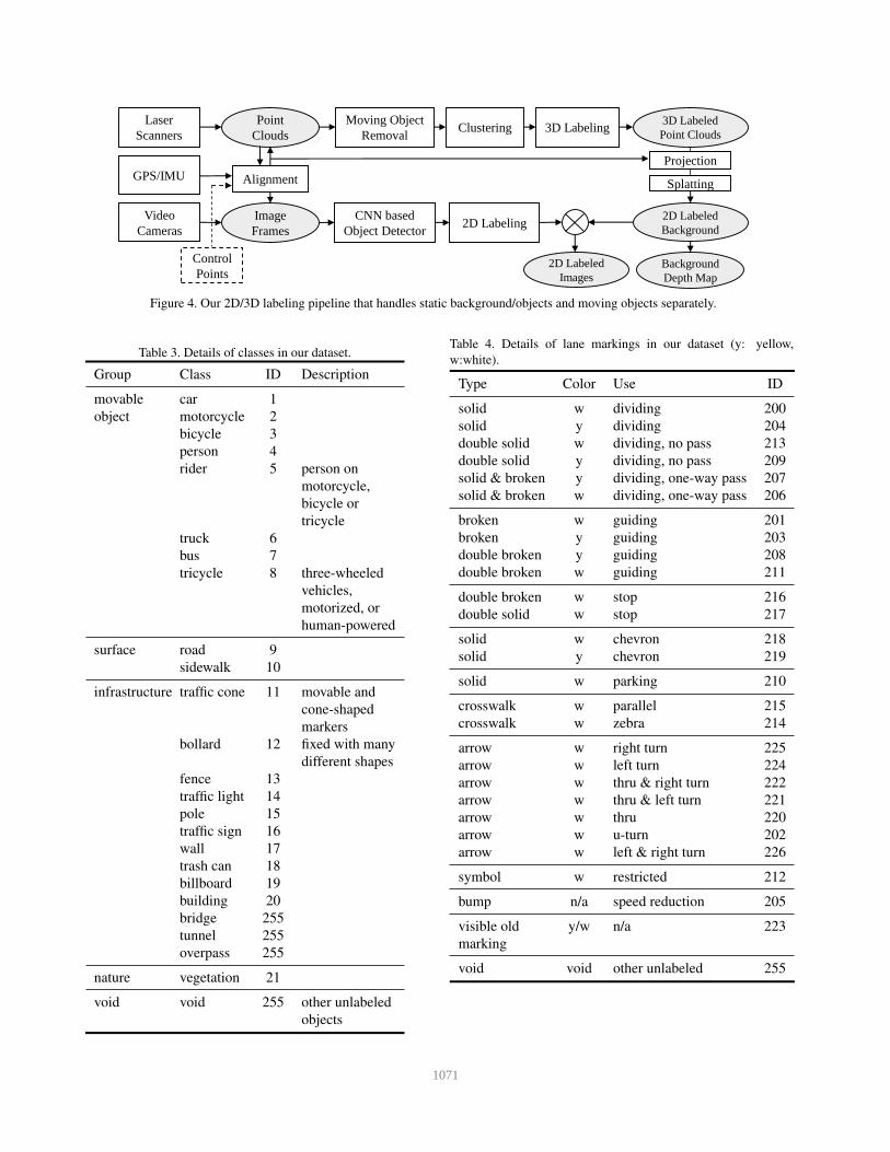
3. In addition to typical object annotations, our dataset

also contains fine grain labelling of lane markings

(with 28 classes).

4. An interactive and efficient 2D/3D joint-labelling

pipeline is designed for this dataset. On average it

saves 70% labeling time. Based on our labelling

pipeline, all the 3D point clouds will be assigned with

above annotations. Therefore, our dataset is the first

open dataset of street views containing 3D annotations.

5. The instance-level annotations are available for video

frames, which are especially useful to design spatial-

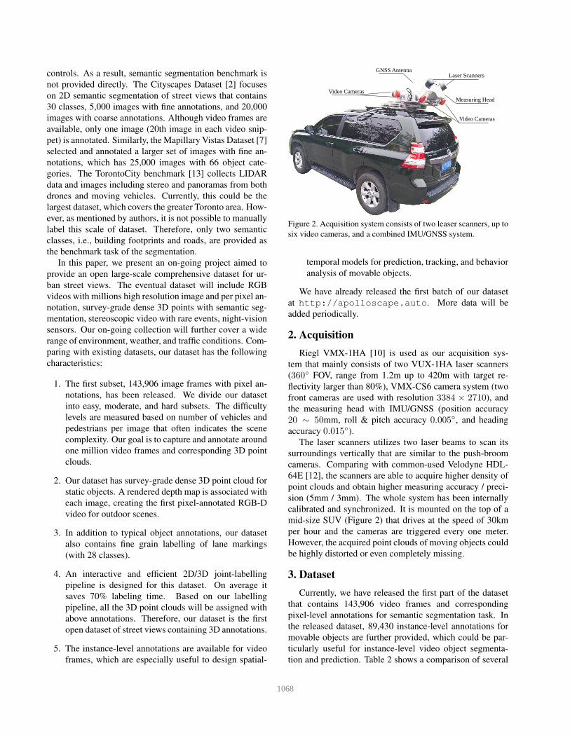
Laser Scanners

Video CamerasMeasuring Head

GNSS Antenna

Video Cameras

Figure 2. Acquisition system consists of two leaser scanners, up to

six video cameras, and a combined IMU/GNSS system.

temporal models for prediction, tracking, and behavior

analysis of movable objects.

We have already released the first batch of our dataset

at http://apolloscape.auto. More data will be

added periodically.

2. Acquisition

Riegl VMX-1HA [10] is used as our acquisition sys-

tem that mainly consists of two VUX-1HA laser scanners

(360◦ FOV, range from 1.2m up to 420m with target re-

flectivity larger than 80%), VMX-CS6 camera system (two

front cameras are used with resolution 3384 × 2710), and

the measuring head with IMU/GNSS (position accuracy

20 ∼ 50mm, roll & pitch accuracy 0.005◦, and heading

accuracy 0.015◦).

The laser scanners utilizes two laser beams to scan its

surroundings vertically that are similar to the push-broom

cameras. Comparing with common-used Velodyne HDL-

64E [12], the scanners are able to acquire higher density of

point clouds and obtain higher measuring accuracy / preci-

sion (5mm / 3mm). The whole system has been internally

calibrated and synchronized. It is mounted on the top of a

mid-size SUV (Figure 2) that drives at the speed of 30km

per hour and the cameras are triggered every one meter.

However, the acquired point clouds of moving objects could

be highly distorted or even completely missing.

3. Dataset

Currently, we have released the first part of the dataset

that contains 143,906 video frames and corresponding

pixel-level annotations for semantic segmentation task. In

the released dataset, 89,430 instance-level annotations for

movable objects are further provided, which could be par-

ticularly useful for instance-level video object segmenta-

tion and prediction. Table 2 shows a comparison of several

1068

Table 1. Total and average number of instances in Kitti,

Cityscapes, and our dataset (instance-level). The letters, e, m, and

h, indicate easy, moderate, and hard subsets respectively.

Count Kitti Cityscapes Ours (instance)

total (×104)

person 0.6 2.4 54.3

vehicle 3.0 4.1 198.9

average per image e m h

person 0.8 7.0 1.1 6.2 16.9

vehicle 4.1 11.8 12.7 24.0 38.1

car - - 9.7 16.6 24.5

motorcycle - - 0.1 0.8 2.5

bicycle - - 0.2 1.1 2.4

rider - - 0.8 3.3 6.3

truck - - 0.8 0.8 1.4

bus - - 0.7 1.3 0.9

tricycle 0 0 0.4 0.3 0.2

key properties between our dataset and other street-view

datasets.

The dataset is collected from different traces that present

easy, moderate, and heavy scene complexities. Similar to

the Cityscapes, we measure the scene complexity based on

the amount of movable objects, such as person and vehi-

cles. Table 1 compares the scene complexities between our

dataset and other open datasets [2, 4]. In the table, we also

show the statistics for the individual classes of movable ob-

jects. We find that both total number and average num-

ber of object instances are much higher than those of other

datasets. More importantly, our dataset contains more chal-

lenging environments are shown in Figure 3. For instance,

two extreme lighting conditions (e.g., dark and bright) ap-

pear in the same image that could be caused by the shadow

of an overpass. Reflections of multiple nearby vehicles on

a bus surface may fail many instance-level segmentation al-

gorithms. We will continue releasing more data in near fu-

ture with large diversities of location, traffic conditions, and

weathers.

3.1. Specifications

We annotate 25 different labels covered by five groups.

Table 3 gives the details of these labels. The IDs shown in

the table are the IDs used for training. The value 255 in-

dicates the ignoring labels that currently are not evaluated

during the testing phase. The specifications of the classes

are similar to the Cityscape dataset with several differences.

For instance, we add one new “tricycle” class that is a quite

popular transport in the east Asia countries. This class cov-

ers all kinds of three-wheeled vehicles that could be both

motorized and human-powered. While the rider class in the

Cityscape is defined as the person on means of transport,

we consider the person and the transport as a single mov-

ing object and merge them together as a single class. The

three classes related to the rider, i.e., bicycle, motorcycle,

and tricycle, represent the empty transports parked along

the roads.

We also annotate 28 different lane markings that cur-

rently are not available in existing open datasets. The anno-

tations are defined based on lane boundary attributes includ-

ing color (e.g., white and yellow) and type (e.g., solid and

broken). Table 4 gives detailed information of these lane

markings. We separate “visible old marking” from other

classes, which represents the “ghost marking” that is vis-

ible remnants of old lane marking. This kind of marking

is a persistent problem in many countries that could cause

confusion even for human drivers.

4. Labeling Process

In order to make our labeling of video frames accurate

and efficient, we develop a labeling pipeline as shown in

Figure 4. The pipeline mainly consists of two stages, 3D la-

beling and 2D labeling, to handle static background/objects

and moving objects respectively. The basic idea of our

pipeline is similar to the one described in [15], while some

key techniques used in our pipeline are different. For in-

stance, the algorithms to handle moving objects are differ-

ent.

The point clouds of moving objects could be highly dis-

torted as mentioned in the Section 2. Therefore, we take

three steps to eliminate this part of point clouds: 1) scan

the same road segment multiple rounds; 2) align these point

clouds; 3) remove the points based on the temporal consis-

tency. Note that additional control points could be added to

further improve alignment performance in the step 2).

In order to speed up the 3D labeling process, we first

over-segment point clouds into point clusters based on spa-

tial distances and normal directions. Then, we label these

point clusters manually. Based on part of labeled data, we

also re-train the PointNet++ model [8] to pre-segment the

point clouds that could achieve better segmentation perfor-

mance. As these preliminary results still cannot be used

directly as the ground truth, we refine the results by fixing

wrong annotations manually. The wrong annotations often

occur around the object boundaries. The 3D labeling tool

is developed to integrate the above modules together. The

user interface design of the tool as shown in Figure 5 fur-

ther speed up the labeling process, which includes 3D ro-

tation, (inverse-)selection by polygons, matching between

point clouds and camera views, and so on.

Once the 3D annotations are generated, the annotations

of static background/objects for all the 2D image frames are

generated automatically by 3D-2D projections. The splat-

ting techniques in computer graphics are further applied to

1069

Figure 3. Some images with challenging environments (center-cropped for visualization purpose). The last row contains enlarged regions

enclosed by yellow rectangles.

Table 2. Comparison between our dataset and the other street-view datasets. “Real data” means whether the data is collected from our

physical world. “3D labels” means whether it contains a 3D map of scenes with semantic label. “2D video labels” means whether it has

per-pixel semantic label. “2D/3D lane labels” means whether it has 3D semantic labels and video per-pixel labels for lane markings.

Dataset Real Data Camera Pose 3D Labels 2D Video Labels 2D/3D Lane Labels

CamVid [1]√

- - - -

Kitti [4]√ √

sparse - -

Cityscapes [2]√

- - selected frames -

Toronto [13]√ √

building & road selected pixels -

Synthia [11] -√

-√ √

P.E.B. [9] -√

-√

-

Ours√ √

dense√ √

handle unlabeled pixels that are often caused by missing

points or strong reflections.

To speed up the 2D labeling process, we first train a CNN

network for movable objects [14] and pre-segment the 2D

images. Another labeling tool for 2D images is developed

to fix or refine the segmentation results. Again, the wrong

annotations often occur around the object boundaries that

could be caused by merge/split of multiple objects and harsh

lighting conditions. Our 2D labeling tool is designed so that

the control points of the boundaries could be easily selected

and adjusted.

Figure 6 presents an example of 2D annotated image.

Notice that some background classes such as fence, traffic

light, and vegetation are able to be annotated in details. In

other datasets, these classes could be ambiguous caused by

occlusions or labeled as a whole region in order to save la-

beling efforts.

5. Benchmark Suite

Given 3D annotations, 2D pixel and instance-level anno-

tations, background depth maps, camera pose information,

a number of tasks could be defined. In current release, we

1070

Laser Scanners

Video Cameras

GPS/IMU

Point Clouds

Image Frames

Moving Object Removal

Clustering 3D Labeling3D Labeled Point Clouds

2D Labeled Background

CNN based Object Detector

2D Labeling

Alignment

Projection

2D Labeled Images

Splatting

Background Depth Map

Control Points

Figure 4. Our 2D/3D labeling pipeline that handles static background/objects and moving objects separately.

Table 3. Details of classes in our dataset.

Group Class ID Description

movable car 1

object motorcycle 2

bicycle 3

person 4

rider 5 person on

motorcycle,

bicycle or

tricycle

truck 6

bus 7

tricycle 8 three-wheeled

vehicles,

motorized, or

human-powered

surface road 9

sidewalk 10

infrastructure traffic cone 11 movable and

cone-shaped

markers

bollard 12 fixed with many

different shapes

fence 13

traffic light 14

pole 15

traffic sign 16

wall 17

trash can 18

billboard 19

building 20

bridge 255

tunnel 255

overpass 255

nature vegetation 21

void void 255 other unlabeled

objects

Table 4. Details of lane markings in our dataset (y: yellow,

w:white).

Type Color Use ID

solid w dividing 200

solid y dividing 204

double solid w dividing, no pass 213

double solid y dividing, no pass 209

solid & broken y dividing, one-way pass 207

solid & broken w dividing, one-way pass 206

broken w guiding 201

broken y guiding 203

double broken y guiding 208

double broken w guiding 211

double broken w stop 216

double solid w stop 217

solid w chevron 218

solid y chevron 219

solid w parking 210

crosswalk w parallel 215

crosswalk w zebra 214

arrow w right turn 225

arrow w left turn 224

arrow w thru & right turn 222

arrow w thru & left turn 221

arrow w thru 220

arrow w u-turn 202

arrow w left & right turn 226

symbol w restricted 212

bump n/a speed reduction 205

visible old y/w n/a 223

marking

void void other unlabeled 255

1071

Figure 5. The user interface of our 3D labeling tool.

Figure 6. An example of 2D annotation with boundaries in details.

mainly focus on the 2D image parsing task. We would like

to add more tasks in near future.

5.1. Image Parsing Metric

Given set of ground truth labels S = {Li}Ni=1and set

of predicted labels S∗ = {Li}Ni=1, the intersect over union

(IoU) metric [3] for a class c is computed as,

IoU(S,S∗, c) =

∑N

i=1tp(i, c)

∑N

i=1(tp(i, c) + fp(i, c) + tn(i, c))

(1)

tp(i, c) =∑

p

1(Li(p) = c · Li(p) = c)

fp(i, c) =∑

p

1(Li(k) 6= c · Li(p) = c)

tn(i, c) =∑

p

1(Li(k) = c · Li(p) 6= c)

Then the overall mean IoU is the average of all C classes:

F(S,S∗) = 1

C

∑c IoU(S,S∗, c).

5.2. Per­frame based evaluation

Tracking information between consecutive frames is not

available in the current release. Therefore, we use per-frame

based evaluation. However, rather than evaluating all the

images together that is same as the evaluation for single im-

age, we consider per-frame evaluation.

5.2.1 Metric for video semantic segmentation

We propose the per-frame IoU metric that evaluates each

predicted frame independently.

Given a sequence of images with ground truth labels

S = {Li}Ni=1and predicted label S∗ = {Li}Ni=1

. Let the

metric between two corresponding images is m(L, L). Each

predicted label L will contain per-pixel prediction.

F(S,S∗) = mean(

∑i m(Li, Li)∑

i Ni

) (2)

m(Li, Li) = [· · · , IoU(Li = j, Li = j), · · · ]T (3)

Ni = [· · · , 1(j ∈ L(Li) or j ∈ L(Li), · · · ] (4)

where IoU is computed between two binary masks that are

obtained by setting Li = j and Li = j. j ∈ L(Li) means

label j appears in the ground truth label Li.

5.3. Metric for video object instance segmentation

We first match between ground truth and predicted in-

stances based on the thresholding of overlapping areas. For

each predicted instance, if the overlapping area between the

predicted instance and the ignoring labels is larger than a

threshold, the predicted instance is removed from the eval-

uation. Notice that the group classes, such as car group and

bicycle group, are also ignored in the evaluation. Predicted

instances that are not matched are counted as false positives.

We use the interpolated average precision (AP) [5] as

the metric for object segmentation. The AP is computed for

each class for all the image frames for each video clip. The

mean AP (mAP) is then computed for all the video clips and

all the classes.

6. Experiment Results for Image Parsing

We conducted our experiments on the Wide ResNet-

38 network [14] that trades depth for width comparing

with the original ResNet structure [6]. The released model

is fine-tuned using our dataset with initial learning rate

0.0001, standard SGD with momentum 0.9 and weight de-

cay 0.0005, random crop with size 512×512, 10 times data

augmentation that includes scaling and left-right flipping,

and 100 epochs. The predictions are computed with one

single scale 1.0 and without any post-processing steps. To

1072

Table 5. Results of image parsing based on ResNet-38 network

using 5K training images.

IoU

Group Class Cityscape Ours

movable car 94.67 87.12

object motorcycle 70.51 27.99

bicycle 78.55 48.65

person 83.17 57.12

rider 65.45 6.58

truck 62.43 25.28

bus 88.61 48.73

mIoU 77.63 43.07

surface road 97.94 92.03

sidewalk 84.08 46.42

infrastructure fence 61.49 42.08

traffic light 70.98 67.49

pole 62.11 46.02

traffic sign 78.93 79.60

wall 58.81 8.41

building 92.66 65.71

nature vegetation 92.41 90.53

be comparable with the training and testing in the ResNet-

38 network, we select a small subset from our dataset that

consists of 5,378 training images and 671 testing images,

which are at the same order of fine labeled images in the

Cityscapes dataset (i.e., around 5K training images and 500

test images). Table 5 shows the parsing results of classes

in common for these two datasets (IoU is computed based

on all frames). Notice that the IoUs computed based on our

dataset are much lower than the IoUs from the Cityscapes.

The mIoU for movable objects in our dataset is 34.6% lower

than the one for the Cityscapes (common classes for both

datasets).

7. Conclusion and Future Work

In this work, we present a large-scale comprehensive

dataset of street views. This dataset contains 1) higher scene

complexities than existing datasets; 2) 2D/3D annotations

and pose information; 3) various annotated lane markings;

4) video frames with instance-level annotations.

In the future, we will first enlarge our dataset to achieve

one million annotated video frames with more diversified

conditions including snow, rain, and foggy environments.

Second, we plan to mount stereo cameras and a panoramic

camera system in near future to generate depth maps and

panoramic images. In the current release, the depth infor-

mation for the moving objects is still missing. We would

like to produce complete depth information for both static

background and moving objects.

References

[1] G. J. Brostow, J. Fauqueur, and R. Cipolla. Semantic object

classes in video: A high-definition ground truth database.

Pattern Recognition Letters, 30(2):88–97, 2009.

[2] M. Cordts, M. Omran, S. Ramos, T. Rehfeld, M. Enzweiler,

R. Benenson, U. Franke, S. Roth, and B. Schiele. The

cityscapes dataset for semantic urban scene understanding.

In Proc. of the IEEE Conference on Computer Vision and

Pattern Recognition (CVPR), 2016.

[3] M. Everingham, S. A. Eslami, L. Van Gool, C. K. Williams,

J. Winn, and A. Zisserman. The pascal visual object classes

challenge: A retrospective. International journal of com-

puter vision, 111(1):98–136, 2015.

[4] A. Geiger, P. Lenz, C. Stiller, and R. Urtasun. Vision meets

robotics: The kitti dataset. International Journal of Robotics

Research (IJRR), 2013.

[5] B. Hariharan, P. Arbelaez, R. Girshick, and J. Malik. Simul-

taneous detection and segmentation. In European Confer-

ence on Computer Vision, pages 297–312. Springer, 2014.

[6] K. He, X. Zhang, S. Ren, and J. Sun. Deep residual learn-

ing for image recognition. In Proceedings of the IEEE con-

ference on computer vision and pattern recognition, pages

770–778, 2016.

[7] G. Neuhold, T. Ollmann, S. R. Bulo, and P. Kontschieder.

The mapillary vistas dataset for semantic understanding of

street scenes. In Proceedings of the International Confer-

ence on Computer Vision (ICCV), Venice, Italy, pages 22–29,

2017.

[8] C. R. Qi, L. Yi, H. Su, and L. J. Guibas. Pointnet++: Deep hi-

erarchical feature learning on point sets in a metric space. In

Advances in Neural Information Processing Systems, pages

5105–5114, 2017.

[9] S. R. Richter, Z. Hayder, and V. Koltun. Playing for bench-

marks. In International Conference on Computer Vision

(ICCV), 2017.

[10] RIEGL. VMX-1HA. http://www.riegl.com/, 2018.

[11] G. Ros, L. Sellart, J. Materzynska, D. Vazquez, and A. M.

Lopez. The synthia dataset: A large collection of synthetic

images for semantic segmentation of urban scenes. In Pro-

ceedings of the IEEE Conference on Computer Vision and

Pattern Recognition, pages 3234–3243, 2016.

[12] Velodyne Lidar. HDL-64E. http://velodynelidar.

com/, 2018. [Online; accessed 01-March-2018].

[13] S. Wang, M. Bai, G. Mattyus, H. Chu, W. Luo, B. Yang,

J. Liang, J. Cheverie, S. Fidler, and R. Urtasun. Torontocity:

Seeing the world with a million eyes. In Proceedings of the

IEEE Conference on Computer Vision and Pattern Recogni-

tion, pages 3009–3017, 2017.

[14] Z. Wu, C. Shen, and A. v. d. Hengel. Wider or deeper: Revis-

iting the resnet model for visual recognition. arXiv preprint

arXiv:1611.10080, 2016.

[15] J. Xie, M. Kiefel, M.-T. Sun, and A. Geiger. Semantic in-

stance annotation of street scenes by 3d to 2d label transfer.

In Proceedings of the IEEE Conference on Computer Vision

and Pattern Recognition, pages 3688–3697, 2016.

1073