Loughborough UniversityInstitutional Repository

The application of porousmedia to simulate theupstream effects of gas

turbine injector swirl vanes

This item was submitted to Loughborough University's Institutional Repositoryby the/an author.

Citation: FORD, C.L., CARROTTE, J.F. and WALKER, A.D., 2013. Theapplication of porous media to simulate the upstream effects of gas turbineinjector swirl vanes. Computers & Fluids, 77, pp. 143-151.

Additional Information:

• This paper was accepted for publication in the journal Comput-ers & Fluids and the definitive published version is available athttp://dx.doi.org/10.1016/j.compfluid.2013.03.001

Metadata Record: https://dspace.lboro.ac.uk/2134/19087

Version: Accepted for publication

Publisher: c© Elsevier

Rights: This work is made available according to the conditions of the Cre-ative Commons Attribution-NonCommercial-NoDerivatives 4.0 International(CC BY-NC-ND 4.0) licence. Full details of this licence are available at:https://creativecommons.org/licenses/by-nc-nd/4.0/

Please cite the published version.

1

The Application of Porous Media to Simulate the Upstream Effects of

Gas Turbine Injector Swirl Vanes

Ford, C. L., Carrotte J. F. and Walker, A. D.

Abstract

Numerical simulations are an invaluable means of evaluating design solutions. This is especially true in the

initial design phase of a project where several simulations may be required as part of an optimisation study. The

design of aircraft gas turbine combustor external aerodynamics frequently calls upon the services of numerical

methods to visualise the existing flow field, and develop architectures which improve the performance of the

system. Many of these performance improvements are driven by the desire to reduce fuel burn and cut emissions

lowering the environmental impact of aviation. The gas turbine combustion chamber is, however, reasonably

complex geometrically and requires a high fidelity model to resolve small geometric details. The fuel injector is

the most geometrically complex component, requiring around 20% of the mesh cells of the entire domain. This

makes it expensive to model in terms of both requisite computational resource and run time. Most modern

aircraft gas turbines utilise swirling flow fields to stabilise the flame front in the combustion liner. The swirl

cone is generally generated using fixed angle vane rows within the injector. It is these small features that are

responsible for the requisite high mesh cell count. This paper presents a numerical method for replacing the

injector swirl vane passages with mathematically porous volumes which replicate the required pressure drop.

Modelling using porous media is preferential to modelling the fully featured injector as it allows a significant

reduction in the size of the computational domain and number of cells. Additionally the simplification makes the

geometry easier to change, scale and re-mesh during development. This in turn allows significant time savings

which serve ultimately to expedite the design process. This method has been rigorously tested through a range

of approach conditions and flow conditions to ensure that it is robust enough for use in the design process. The

loss in accuracy owing to the simplification has been demonstrated to be less than 4.4%, for all tested flow

fields. This error is dependent on the flow conditions and is generally much less for passages fed with

representative levels of upstream distortion.

2

Nomenclature

𝐴1 Geometric inlet area (vane passage)

𝐴2 Geometric outlet area (vane passage)

𝐵 Blockage ratio

𝐶 Total velocity magnitude

c Swirl vane chord

𝐷𝑖 Pipe inner diameter

𝐷𝑖𝑗 Viscous loss coefficient

𝐷𝑜 Pipe outer diameter

𝐸 Average velocity magnitude error

𝑓 Frequency of distorted profile

ℎ Height of distorted profile

𝐾𝑥 Axial Porous loss coefficient

𝐾𝜃 Tangential Porous loss coefficient

𝐿 Porous media axial length

𝑝 Static pressure

𝑃 Total pressure

𝑞 Dynamic pressure

𝑆𝑖 Momentum sink scalar

𝑢 Axial velocity component

𝑢ℎ Maximum inlet profile velocity

𝑣𝜃 Tangential velocity component

𝛾1 PM/vane leading edge swirl angle

𝛾2 Vane exit swirl angle

𝛾2′ PM exit swirl angle

𝜃𝑥 Ratio of Kθ to Kx

𝜆 Total pressure loss coefficient

𝜇 Fluid dynamic viscosity

𝜌 Fluid density

3

Subscripts

𝑣 Referring to vaned geometry

𝑚 Referring to Porous media

Superscripts

� Area weighted spatial mean value

� Mass weighted spatial mean value

4

1.0 Introduction

In aero-style gas turbine combustion systems the velocity of the flow issuing from the upstream compressor

spool must be reduced and the flow distributed to the various flame tube features. These external aerodynamic

processes are typically achieved using a dump diffuser type architecture in which an annular diffuser is followed

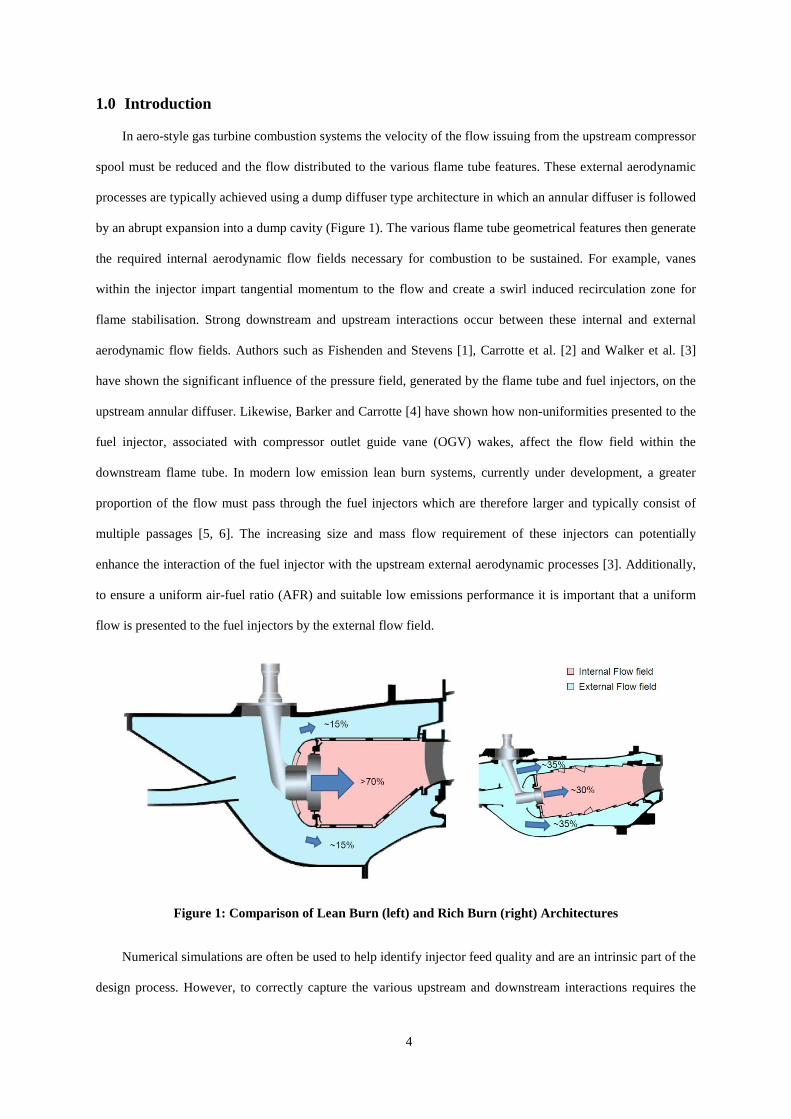
by an abrupt expansion into a dump cavity (Figure 1). The various flame tube geometrical features then generate

the required internal aerodynamic flow fields necessary for combustion to be sustained. For example, vanes

within the injector impart tangential momentum to the flow and create a swirl induced recirculation zone for

flame stabilisation. Strong downstream and upstream interactions occur between these internal and external

aerodynamic flow fields. Authors such as Fishenden and Stevens [1], Carrotte et al. [2] and Walker et al. [3]

have shown the significant influence of the pressure field, generated by the flame tube and fuel injectors, on the

upstream annular diffuser. Likewise, Barker and Carrotte [4] have shown how non-uniformities presented to the

fuel injector, associated with compressor outlet guide vane (OGV) wakes, affect the flow field within the

downstream flame tube. In modern low emission lean burn systems, currently under development, a greater

proportion of the flow must pass through the fuel injectors which are therefore larger and typically consist of

multiple passages [5, 6]. The increasing size and mass flow requirement of these injectors can potentially

enhance the interaction of the fuel injector with the upstream external aerodynamic processes [3]. Additionally,

to ensure a uniform air-fuel ratio (AFR) and suitable low emissions performance it is important that a uniform

flow is presented to the fuel injectors by the external flow field.

Figure 1: Comparison of Lean Burn (left) and Rich Burn (right) Architectures

Numerical simulations are often be used to help identify injector feed quality and are an intrinsic part of the

design process. However, to correctly capture the various upstream and downstream interactions requires the

5

external and internal aerodynamic processes to be simulated, see for example Lazik et al. [6]. This

computationally expensive, additionally the modelling methods used to simulate the external aerodynamics are

less suitable for the internal aerodynamic processes and vice-versa. It is, of course possible to model the external

or internal flow field separately. When examining the external flow field only, the fuel injector may be replaced

by appropriate exit boundary conditions. This approach was used by Walker [7] to develop a novel combustor

pre-diffuser. However, this methodology will not correctly capture the upstream effect of the pressure field

associated with the aerodynamic processes undertaken by the flow passing through the injector swirl vanes and

into the flame tube and is therefore unlikely to be accurate in the injector near field.

A large injector pressure drop, whilst being detrimental to the engine cycle, would result in an upstream

pressure field that causes the flow to redistribute and reduce the magnitude of any spatial variations in the

pressure and velocity of the flow presented to the injector. This is a prime example of the interaction which

exists between downstream processes and the approaching flow. It is crucial to capture these interactions

correctly in order that the flow distribution entering the swirl vanes is correctly simulated. Hence the potential

magnitude of any spatial AFR variations in the downstream flow field can be assessed.

This paper describes a numerical methodology which allows the injector swirl vane geometry and

downstream flame tube to be replaced with a volume that is mathematically designated porous [8]. In this way

the correct gross static pressure field at the leading edge of the injector swirl vanes can be generated. This is

effectively achieved by creating a pressure drop that broadly mimics that which would occur within the injector

swirl vanes and downstream flame tube. By utilising this approach the need to model the downstream geometry

and the associated complexities are avoided. The methodology is easy to employ and since the vane passage is

replaced by a prismatic volume it is easy to scale, adjust and re-mesh. All of these advantages result in a shorter

simulation time, which in the context of initial design iterations may result in a significant shortening of the

design process.

6

2.0 Porous Medium Methodology

2.1 System Pressure Losses

Based on a simple 1D analysis, the change in pressure incurred by a stream tube as it passes through a

typical gas turbine combustion system is considered (Figure 2). Aerodynamic processes external to the flame

tube result in changes to both total and static pressure. Through the diffuser and dump cavity regions a reduction

in total pressure is observed which is accompanied, in general, by an increase in static pressure. Upon entering

the injector swirl vane passages the static pressure is then reduced, mainly due to flow acceleration (although a

small reduction associated with a drop in total pressure will also occur). It is assumed that at exit of the injector

the flow undergoes a sudden expansion, with all the kinetic energy being converted into turbulence at some

downstream location.

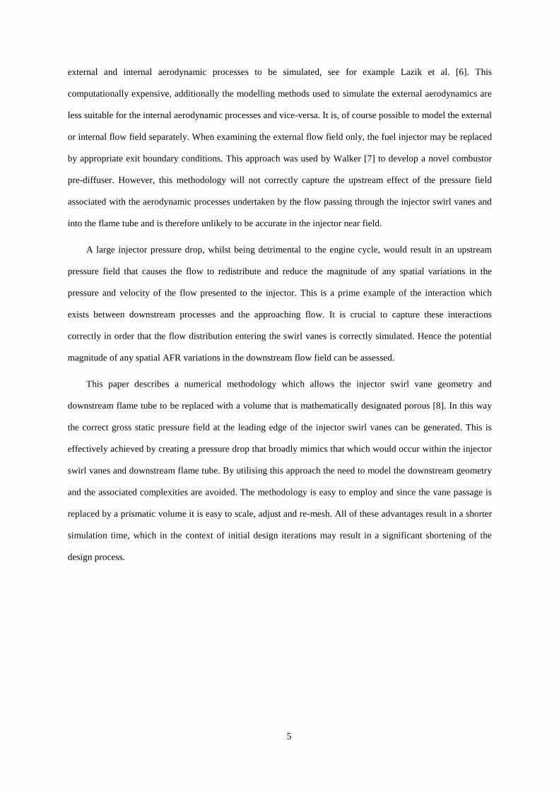
Figure 2: Pressure Variation through the System (A) Fully Featured, (B) With Porous Media

With reference to Figure 2, the total system pressure loss can be expressed in terms of the losses incurred

by the flow in the various regions:

∆𝑃𝐴(0−3) = ∆𝑃(0−1) + ∆𝑃(1−2)+∆𝑃(2−3) Eqn. 1

This may be re-written as:

∆𝑃𝐴(0−3) = ∆𝑃(0−1) + ∆𝑝𝑣 + 𝑞1 Eqn. 2

Where ∆𝑝𝑣 is the change in static pressure across the vane passage, and 𝑞1 is the dynamic head at the swirl

vane entry plane. If the vane passage and downstream regions within the combustor (1-3) are replaced by a

7

porous medium (Figure 2B) such that the conditions at inlet to the vane passage (1) replicate those that would

occur in the complete (vane passage and combustor) system, the losses may be expressed as:

∆𝑃𝐵(0−2) = ∆𝑃(0−1) + ∆𝑃𝑚 Eqn. 3

The magnitude of the total pressure drop across the porous medium must therefore equal the static pressure

drop within the injector vane passages, plus the vane inlet dynamic head:

∆𝑃𝑚 = ∆𝑝𝑣 + 𝑞1 Eqn. 4

2.2 Injector Swirl Vane Geometry

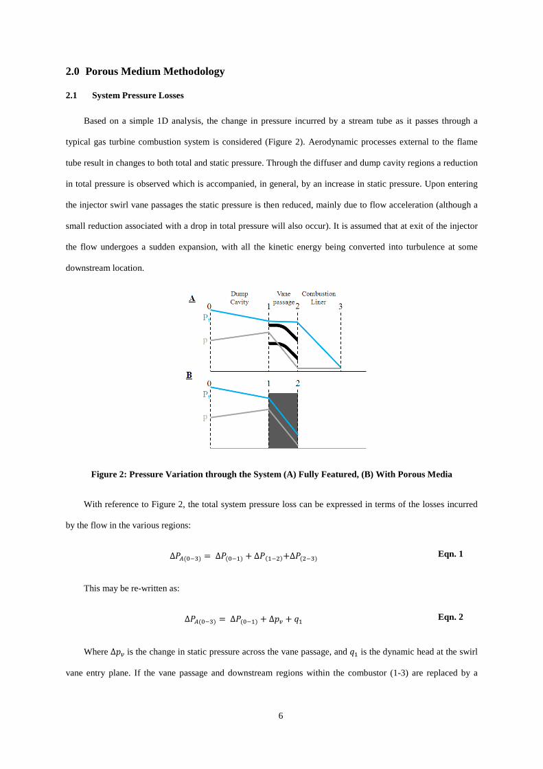
The flow within the vane passage, at a plane of constant radius, is shown in Figure 3. At inlet and exit the

flow velocities and angles are: 𝐶1, 𝐶2, 𝛾1 and 𝛾2 respectively. If it is assumed that the total pressure loss between

stations 1 and 2 is given by ∆𝑃𝑣 then, for incompressible flow:

𝑝1 − 𝑝2 = ∆𝑝𝑣 =𝜌2

(𝐶22 − 𝐶12) + ∆𝑃𝑣 Eqn. 5

Which may be expressed as:

∆𝑝𝑣 =𝑢12𝜌

2��𝐴1 sec 𝛾2𝐴2𝐵

�2

− 𝑠𝑒𝑐2𝛾1� + ∆𝑃𝑣 Eqn. 6

The geometric inlet and exit areas are denoted by A1 and A2 respectively and B is a blockage ratio which

expresses the ratio of effective to geometric area at vane exit, accounting for the finite thickness of the boundary

layers etc. In reality the value of B is small and can be typically set to 1.0 (as in the subsequent results that are

presented) but it has been included here for completeness.

Figure 3: Swirl Vane Schematic

8

2.3 Derivation of PM Loss Coefficients

In most CFD codes a volume may be specified as a porous medium (PM) which acts as a user defined

momentum sink. This is typically composed of losses associated with viscous and inertial components. Since it

is only necessary to replicate a loss value either of these terms can be used. Hence to reduce mathematical

complexity the methodology presented here is based on using the inertial losses only. However, this is also

thought more appropriate for the fully turbulent flows being considered. In this case, the momentum sink term,

S is given by [8]:

𝑆𝑖 = −12�𝐾𝑗𝜌𝐶𝑣𝑗

3

𝑗=1

Eqn. 7

The porous medium is fully defined by the three coefficient terms: Kx, Kr, Kθ, where the subscripts x, r and

θ refer to the axial, radial and tangential directions respectively (relative to an axis defined through the injector

centreline). In fuel injector swirl passages there are generally negligible effects associated with the radial

velocity component thus it has been assumed that this can be ignored (i.e. Kr =0.0).

Since it is only necessary to replicate a loss it could be assumed that it is only necessary to consider the

axial loss coefficient. Reduction to a one dimensional form significantly reduces the mathematical complexity.

However, it will be subsequently shown that the one dimensional form is less appropriate for the flows

considered and for higher accuracy a two dimensional formulation is necessary. Generally, the two loss

components may be in any given ratio, therefore to allow the closure of the equation, the ratio, θk is introduced

to relate the tangential to axial coefficients:

∆𝑃𝑚 =𝜌𝐾𝑥

2�𝐶(𝑢 𝑑𝑥 + 𝜃𝑘𝑣𝜃𝑟𝑑𝜃)𝐿

0

Eqn. 8

Where:

𝜃𝑘 =𝐾𝜃𝐾𝑥

Eqn. 9

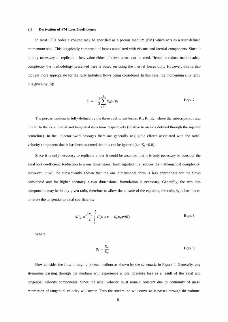
Now consider the flow through a porous medium as shown by the schematic in Figure 4. Generally, any

streamline passing through the medium will experience a total pressure loss as a result of the axial and

tangential velocity components. Since the axial velocity must remain constant due to continuity of mass,

retardation of tangential velocity will occur. Thus the streamline will curve as it passes through the volume.

9

Assuming the inlet flow angle is given by 𝛾1 and the media outlet angle by 𝛾2′ a relationship for the total

pressure loss may be derived as a function of the velocity, media coefficients, and local flow angle, 𝛾(𝑥).

Assuming that the axial velocity is invariant within the PM and substituting tangential terms for their axial

counterparts it is possible to write:

∆𝑃𝑚 =𝜌𝐾𝑥𝑢12

2�{(1 − 𝜃𝑘) sec 𝛾 + 𝜃𝑘𝑠𝑒𝑐3𝛾}𝑑𝑥𝐿

0

Eqn. 10

Figure 4: Porous Medium Schematic

Recall that, as shown by Equation 4, the total pressure loss of the porous section should be equal to the

static pressure drop across the vanes plus the dynamic pressure at inlet. Combining Equations 6 and 10, and re-

arranging, an equation for the value of Kx can be derived, viz:

𝐾𝑥 =𝑘0𝑠𝑒𝑐2𝛾1

∫ {(1 − 𝜃𝑘) sec 𝛾 + 𝜃𝑘𝑠𝑒𝑐3𝛾}𝑑𝑥𝐿0

Eqn. 11

Where:

𝑘0 = �𝐴1 cos 𝛾1𝐴2𝐵 cos 𝛾2

�2

+∆𝑃𝑣𝑞1

Eqn. 12

In the case of pure axial inlet flow (𝛾1 = 0), Equation 11 simply reduces to: 𝐾𝑥 = 𝑘0𝐿

. However, in the

general case an estimation of the behaviour of the flow angle through the PM is required. A good approximation

has been found to be given by:

𝛾 ≈ 𝛾1𝑒𝛤𝑜𝑥 Eqn. 13

Where: 𝛤o is a constant given by:

10

𝛤𝑜 =1𝐿

ln�𝛾2′

𝛾1� |𝛾1 ≠ 0 Eqn. 14

Thus the integrand in the denominator of Equation 11 becomes:

� {(1 − 𝜃𝑘) sec 𝛾+𝜃𝑘𝑠𝑒𝑐3𝛾} 𝑑𝑥𝐿

0≈

1𝛤𝑜�

(1 − 𝜃𝑘) sec 𝛾+𝜃𝑘𝑠𝑒𝑐3𝛾𝛾

𝑑𝛾𝛾2′

𝛾1 Eqn. 15

2.4 Implementation

Achieving an analytical solution for Equation 15 is problematic and the integration can only be practically

achieved numerically. The “gamma approximation” results in a small error in the prediction of K, the magnitude

of which will depend on the flow conditions. This is because the assumed gamma profile only ever utilises the

inlet and outlet angles and the rate of turning is never correctly captured. However, at small inlet angles (less

than around 20º) the error in K is negligibly small (less than 1%). The error increases when a higher range of

approach angles are experienced but has been shown to be less than 3% under all tested conditions. The velocity

profiles generated with the porous medium employed are not so sensitive to the value of K and this

approximation error is negligible.

With knowledge of the geometric areas of the vane passage and the swirl vane angles it is possible to

calculate the approximate value of Kx required. The approach and exit angles may be solved iteratively, by

initially assuming a zero value, i.e. 𝛾1 = 0, then correcting the value of Kx using the mass weighted average

approach and PM exit angles, numerically integrating Equation 15 to find a value of the denominator of

Equation 11. The iterative procedure required for correct use of the porous medium is not as arduous as it may

appear, with solutions tending to converge rapidly after an adjustment in K. Typically only a single iteration is

required. For small inlet angles (<5o) the zero inlet angle assumption is usually suitably accurate.

Initial vaned results suggested that the total pressure loss term: ∆𝑃𝑣𝑞1

(in Equation 12) was typically about 0.6

over a range of inlet conditions and this value was therefore adopted. Furthermore the most accurate value of θk

was found to be 1.0, meaning that the axial and tangential loss coefficients were of equal magnitude. A fuller

examination of the sensitivity of the K equation to the various terms will be subsequently discussed.

11

3.0 Proof of Concept

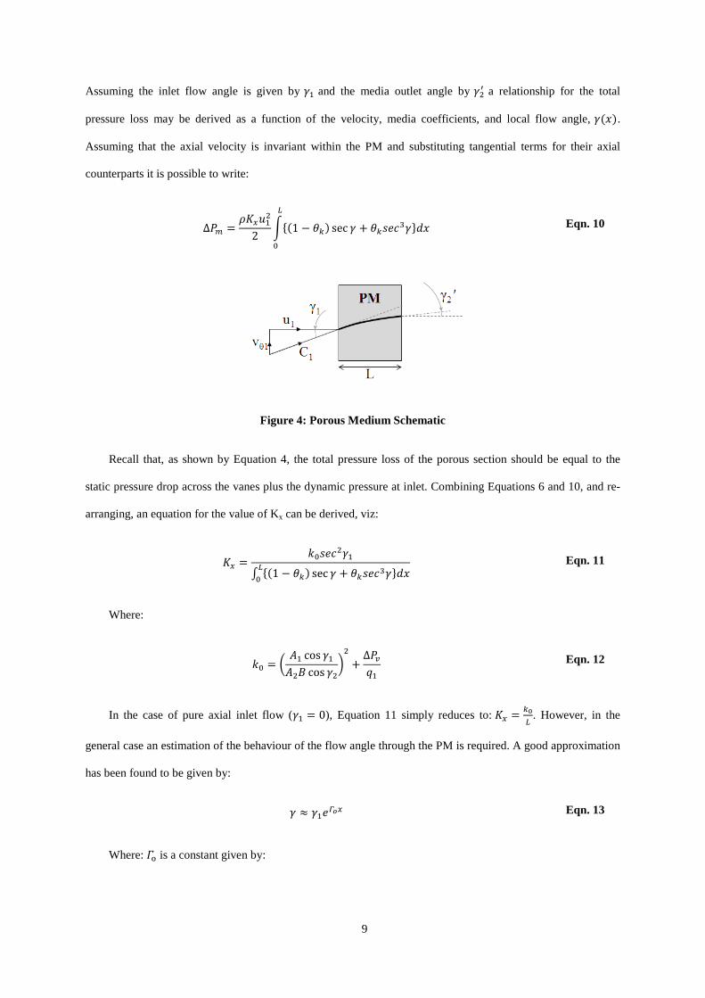
The robustness of the methodology was tested using a simplified model prior to applying it to a more

engine representative configuration. The basic model utilised an annular pipe into which a set of swirl vanes

could be located or the vanes could be replaced with a porous media. The swirl vanes are typical of those found

within modern combustion systems and the duct inlet and exit sections corresponding to approximately 6 and 12

vane chord lengths. Both the inlet and outlet sections had zero wall shear stress to eliminate the influence of any

boundary layer growth on the vane flow. When replacing the vanes with a PM the outlet section was

unnecessary and the outflow boundary was simply placed at the termination of the PM. Calculations were also

undertaken with the PM loss coefficients set to zero. This is equivalent to modelling the injector without any

influence of the vane pressure drop and is typical of current practice. Calculation times were reduced by a factor

of greater than 100 with the vanes replaced by the PM. (For example, using a single processor on a standard

desktop computer simulations times were reduced from more than 24 hours to of order minutes).

Figure 5: Vaned “Pipe” Geometry and PM Equivalent

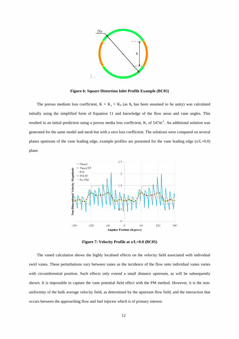
In gas turbine combustion systems the fuel injector will, in general, not be uniformly fed. To make the

proof of concept calculations more realistic various distorted axial velocity profiles were presented to the

vanes/PM. In the first instance the inlet profile was set as a simple square wave with the maxima located at the 3

and 9 o’clock positions consistent with a pronounced pre-diffuser footprint (subsequently dubbed boundary

condition 5 - BC05). The distortion was controlled by varying the magnitude of maximum to average axial

velocity (𝑢ℎ/𝑢�), and the ratio of the height of the wave to the outer diameter of the pipe (h/Do), see Figure 6.

12

Figure 6: Square Distortion Inlet Profile Example (BC05)

The porous medium loss coefficient, K = Kx = Kθ (as θk has been assumed to be unity) was calculated

initially using the simplified form of Equation 11 and knowledge of the flow areas and vane angles. This

resulted in an initial prediction using a porous media loss coefficient, K, of 547m-1. An additional solution was

generated for the same model and mesh but with a zero loss coefficient. The solutions were compared on several

planes upstream of the vane leading edge, example profiles are presented for the vane leading edge (x/L=0.0)

plane.

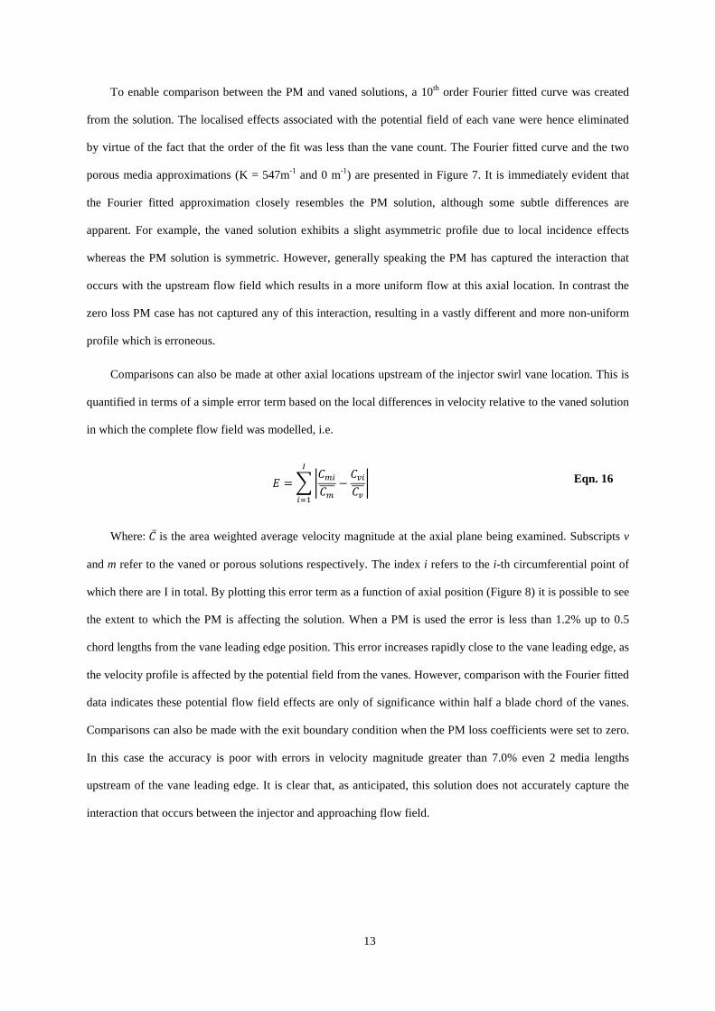
Figure 7: Velocity Profile at x/L=0.0 (BC05)

The vaned calculation shows the highly localised effects on the velocity field associated with individual

swirl vanes. These perturbations vary between vanes as the incidence of the flow onto individual vanes varies

with circumferential position. Such effects only extend a small distance upstream, as will be subsequently

shown. It is impossible to capture the vane potential field effect with the PM method. However, it is the non-

uniformity of the bulk average velocity field, as determined by the upstream flow field, and the interaction that

occurs between the approaching flow and fuel injector which is of primary interest.

13

To enable comparison between the PM and vaned solutions, a 10th order Fourier fitted curve was created

from the solution. The localised effects associated with the potential field of each vane were hence eliminated

by virtue of the fact that the order of the fit was less than the vane count. The Fourier fitted curve and the two

porous media approximations (K = 547m-1 and 0 m-1) are presented in Figure 7. It is immediately evident that

the Fourier fitted approximation closely resembles the PM solution, although some subtle differences are

apparent. For example, the vaned solution exhibits a slight asymmetric profile due to local incidence effects

whereas the PM solution is symmetric. However, generally speaking the PM has captured the interaction that

occurs with the upstream flow field which results in a more uniform flow at this axial location. In contrast the

zero loss PM case has not captured any of this interaction, resulting in a vastly different and more non-uniform

profile which is erroneous.

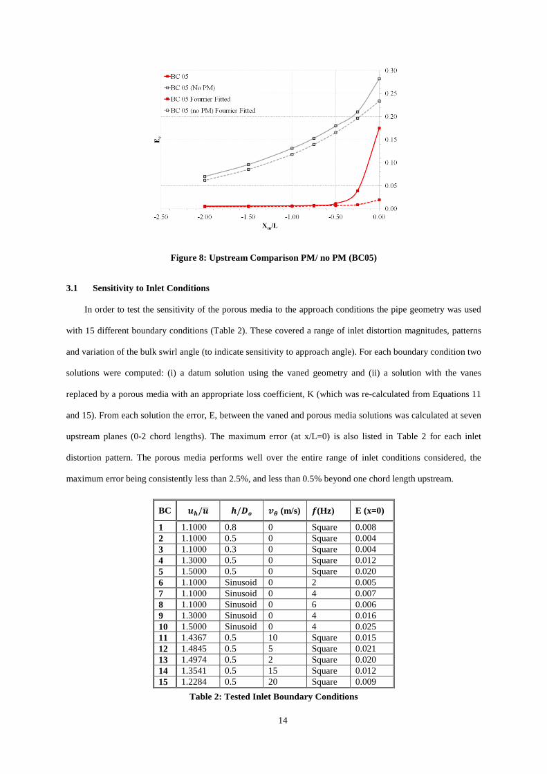
Comparisons can also be made at other axial locations upstream of the injector swirl vane location. This is

quantified in terms of a simple error term based on the local differences in velocity relative to the vaned solution

in which the complete flow field was modelled, i.e.

𝐸 = ��𝐶𝑚𝑖𝐶𝑚����

−𝐶𝑣𝑖𝐶𝑣����

𝐼

𝑖=1

Eqn. 16

Where: 𝐶̅ is the area weighted average velocity magnitude at the axial plane being examined. Subscripts v

and m refer to the vaned or porous solutions respectively. The index i refers to the i-th circumferential point of

which there are I in total. By plotting this error term as a function of axial position (Figure 8) it is possible to see

the extent to which the PM is affecting the solution. When a PM is used the error is less than 1.2% up to 0.5

chord lengths from the vane leading edge position. This error increases rapidly close to the vane leading edge, as

the velocity profile is affected by the potential field from the vanes. However, comparison with the Fourier fitted

data indicates these potential flow field effects are only of significance within half a blade chord of the vanes.

Comparisons can also be made with the exit boundary condition when the PM loss coefficients were set to zero.

In this case the accuracy is poor with errors in velocity magnitude greater than 7.0% even 2 media lengths

upstream of the vane leading edge. It is clear that, as anticipated, this solution does not accurately capture the

interaction that occurs between the injector and approaching flow field.

14

Figure 8: Upstream Comparison PM/ no PM (BC05)

3.1 Sensitivity to Inlet Conditions

In order to test the sensitivity of the porous media to the approach conditions the pipe geometry was used

with 15 different boundary conditions (Table 2). These covered a range of inlet distortion magnitudes, patterns

and variation of the bulk swirl angle (to indicate sensitivity to approach angle). For each boundary condition two

solutions were computed: (i) a datum solution using the vaned geometry and (ii) a solution with the vanes

replaced by a porous media with an appropriate loss coefficient, K (which was re-calculated from Equations 11

and 15). From each solution the error, E, between the vaned and porous media solutions was calculated at seven

upstream planes (0-2 chord lengths). The maximum error (at x/L=0) is also listed in Table 2 for each inlet

distortion pattern. The porous media performs well over the entire range of inlet conditions considered, the

maximum error being consistently less than 2.5%, and less than 0.5% beyond one chord length upstream.

BC 𝒖𝒉/𝒖� 𝒉/𝑫𝒐 𝒗𝜽 (m/s) 𝒇(Hz) E (x=0)

1 1.1000 0.8 0 Square 0.008 2 1.1000 0.5 0 Square 0.004 3 1.1000 0.3 0 Square 0.004 4 1.3000 0.5 0 Square 0.012 5 1.5000 0.5 0 Square 0.020 6 1.1000 Sinusoid 0 2 0.005 7 1.1000 Sinusoid 0 4 0.007 8 1.1000 Sinusoid 0 6 0.006 9 1.3000 Sinusoid 0 4 0.016 10 1.5000 Sinusoid 0 4 0.025 11 1.4367 0.5 10 Square 0.015 12 1.4845 0.5 5 Square 0.021 13 1.4974 0.5 2 Square 0.020 14 1.3541 0.5 15 Square 0.012 15 1.2284 0.5 20 Square 0.009

Table 2: Tested Inlet Boundary Conditions

15

3.2 Sensitivity to Terms in the K Equation

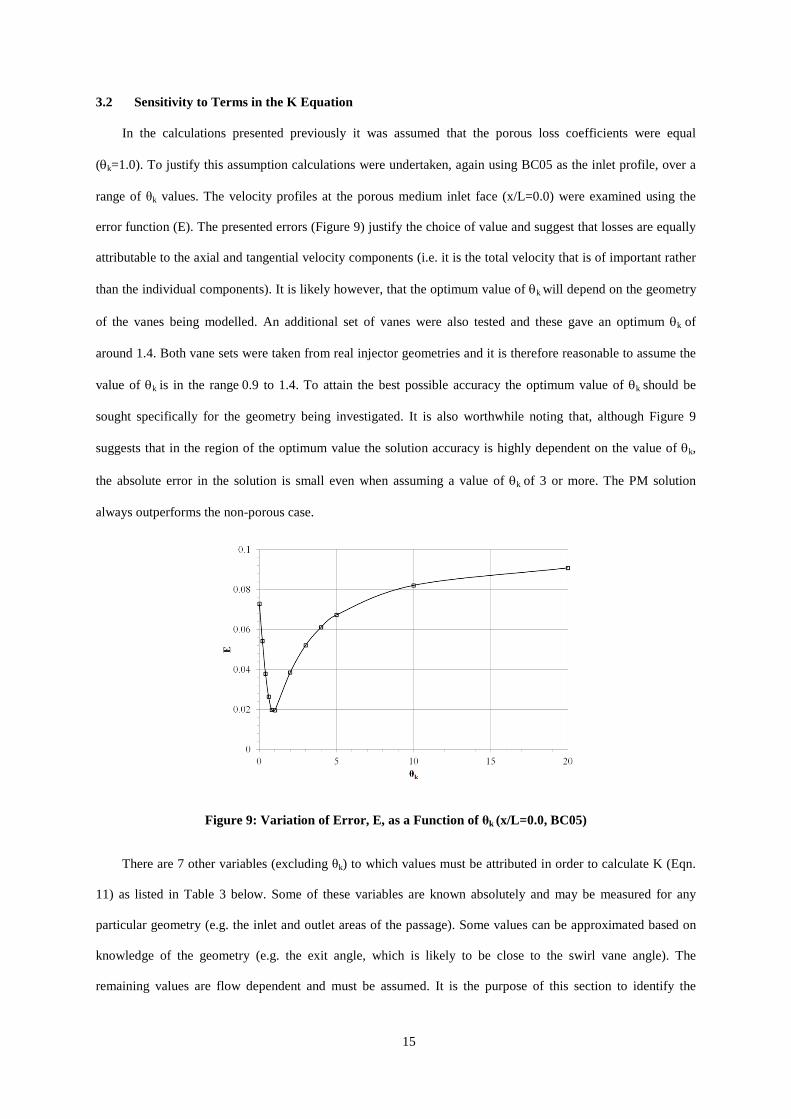
In the calculations presented previously it was assumed that the porous loss coefficients were equal

(θk=1.0). To justify this assumption calculations were undertaken, again using BC05 as the inlet profile, over a

range of θk values. The velocity profiles at the porous medium inlet face (x/L=0.0) were examined using the

error function (E). The presented errors (Figure 9) justify the choice of value and suggest that losses are equally

attributable to the axial and tangential velocity components (i.e. it is the total velocity that is of important rather

than the individual components). It is likely however, that the optimum value of θk will depend on the geometry

of the vanes being modelled. An additional set of vanes were also tested and these gave an optimum θk of

around 1.4. Both vane sets were taken from real injector geometries and it is therefore reasonable to assume the

value of θk is in the range 0.9 to 1.4. To attain the best possible accuracy the optimum value of θk should be

sought specifically for the geometry being investigated. It is also worthwhile noting that, although Figure 9

suggests that in the region of the optimum value the solution accuracy is highly dependent on the value of θk,

the absolute error in the solution is small even when assuming a value of θk of 3 or more. The PM solution

always outperforms the non-porous case.

Figure 9: Variation of Error, E, as a Function of θk (x/L=0.0, BC05)

There are 7 other variables (excluding θk) to which values must be attributed in order to calculate K (Eqn.

11) as listed in Table 3 below. Some of these variables are known absolutely and may be measured for any

particular geometry (e.g. the inlet and outlet areas of the passage). Some values can be approximated based on

knowledge of the geometry (e.g. the exit angle, which is likely to be close to the swirl vane angle). The

remaining values are flow dependent and must be assumed. It is the purpose of this section to identify the

16

sensitivity of the solution to the values chosen. In order to do this, the pipe geometry will be utilised. It is likely

that the actual sensitivity may have some dependency on the geometry being considered. However, the

simplicity of the case allows the effect of the various terms to be investigated much more readily than in a full

engine geometry.

Term Symbol Comment Value PM Length 𝐿 Defined by user Measurable Geometric inlet Area 𝐴1 Known Measureable Geometric Outlet Area 𝐴2 Known Measureable BL blockage 𝐵 Flow dependant 0.99 to 1 Inlet Angle 𝛾1 Flow dependant 0 to 60o Exit Angle 𝛾2 Approximately Known swirl vane angle +/- 5o Vane Total Pressure Loss ∆𝑃𝑣 𝑞1� Flow dependant 0 to 1

Table 3: K Equation Variables and Approximate Values

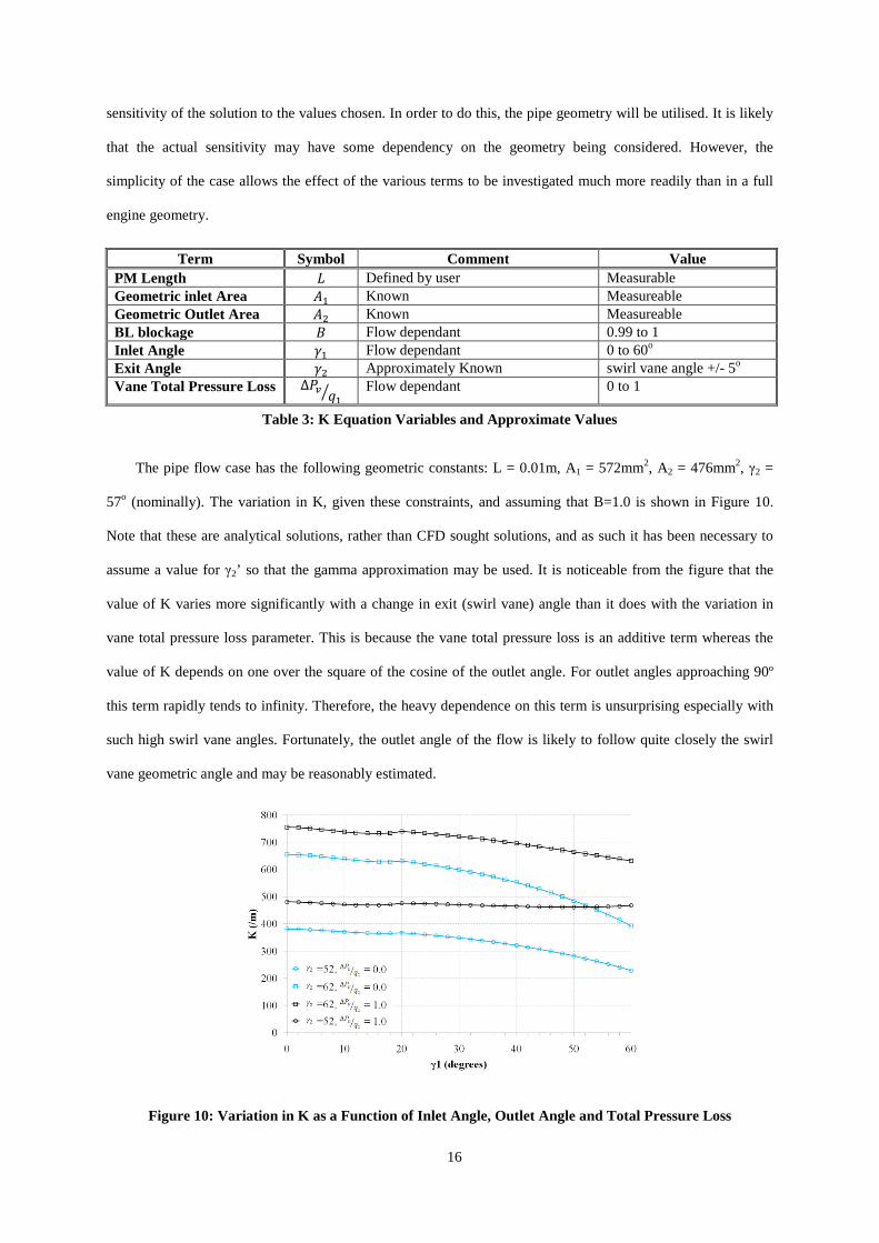
The pipe flow case has the following geometric constants: L = 0.01m, A1 = 572mm2, A2 = 476mm2, γ2 =

57o (nominally). The variation in K, given these constraints, and assuming that B=1.0 is shown in Figure 10.

Note that these are analytical solutions, rather than CFD sought solutions, and as such it has been necessary to

assume a value for γ2’ so that the gamma approximation may be used. It is noticeable from the figure that the

value of K varies more significantly with a change in exit (swirl vane) angle than it does with the variation in

vane total pressure loss parameter. This is because the vane total pressure loss is an additive term whereas the

value of K depends on one over the square of the cosine of the outlet angle. For outlet angles approaching 90º

this term rapidly tends to infinity. Therefore, the heavy dependence on this term is unsurprising especially with

such high swirl vane angles. Fortunately, the outlet angle of the flow is likely to follow quite closely the swirl

vane geometric angle and may be reasonably estimated.

Figure 10: Variation in K as a Function of Inlet Angle, Outlet Angle and Total Pressure Loss

17

For a specific boundary condition case (BC05) which is likely to be reasonably representative of a realistic

geometry the effect of changing the assumed variables was considered. There are many variables so in order to

cut down the amount of investigation two “corner points” were investigated: (i) K=381 m-1, which is equivalent

to a 52º exit angle and a zero total pressure loss vane cascade, and (ii) K=755 m-1, which represents a 62 degree

outlet angle and a total pressure loss equivalent to the inlet dynamic head. These points represent the extremes

of the envelope of K values. Running simulations with these values for K will allow an examination of the

sensitivity of the velocity field to the value of K.

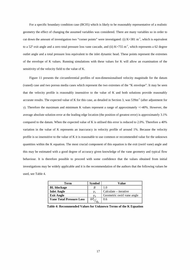
Figure 11 presents the circumferential profiles of non-dimensionalised velocity magnitude for the datum

(vaned) case and two porous media cases which represent the two extremes of the “K envelope”. It may be seen

that the velocity profile is reasonably insensitive to the value of K and both solutions provide reasonably

accurate results. The expected value of K for this case, as detailed in Section 3, was 539m-1 (after adjustment for

γ). Therefore the maximum and minimum K values represent a range of approximately +/-40%. However, the

average absolute solution error at the leading edge location (the position of greatest error) is approximately 3.1%

compared to the datum. When the expected value of K is utilised this error is reduced to 2.0%. Therefore a 40%

variation in the value of K represents an inaccuracy in velocity profile of around 1%. Because the velocity

profile is so insensitive to the value of K it is reasonable to use common or recommended value for the unknown

quantities within the K equation. The most crucial component of this equation is the exit (swirl vane) angle and

this may be estimated with a good degree of accuracy given knowledge of the vane geometry and typical flow

behaviour. It is therefore possible to proceed with some confidence that the values obtained from initial

investigations may be widely applicable and it is the recommendation of the authors that the following values be

used, see Table 4.

Term Symbol Value BL blockage 𝐵 1.0 Inlet Angle 𝛾1 Calculate – iterative Exit Angle 𝛾2 Geometric swirl vane angle Vane Total Pressure Loss ∆𝑃𝑣 𝑞1� 0.6

Table 4: Recommended Values for Unknown Terms of the K Equation

18

Figure 11: Variation in Velocity Profile with K (x/L=0.0, BC05)

4.0 Application to Engine Representative Combustion System Geometry

The main aim of the current work was to establish the porous media methodology for modelling fuel

injector swirl vanes in realistic gas turbine combustors thereby saving valuable time in the preliminary design

process. The final stage in validating the methodology was therefore to apply it to a representative geometry for

which a fully featured and complete CFD solution existed. The model extends from OGV exit, through the pre-

diffuser and into the dump region whilst also including two annuli surrounding the flame tube. The annuli are

truncated and are merely present to provide the correct mass flow distribution within the system, rather than to

specifically investigate the annulus flows. The injector external geometry is common between both cases but the

internal geometry and downstream flame tube depends on whether a fully featured or porous media approach is

used. In the baseline case all the significant features of the injector and downstream combustor are modelled.

However, in the porous case the vanes within each injector passage are replaced by porous media (starting at the

leading edge position and extending approximately one chord downstream). Each injector passage has an

individual exit boundary which may be used to adjust the mass flow split between the different injector

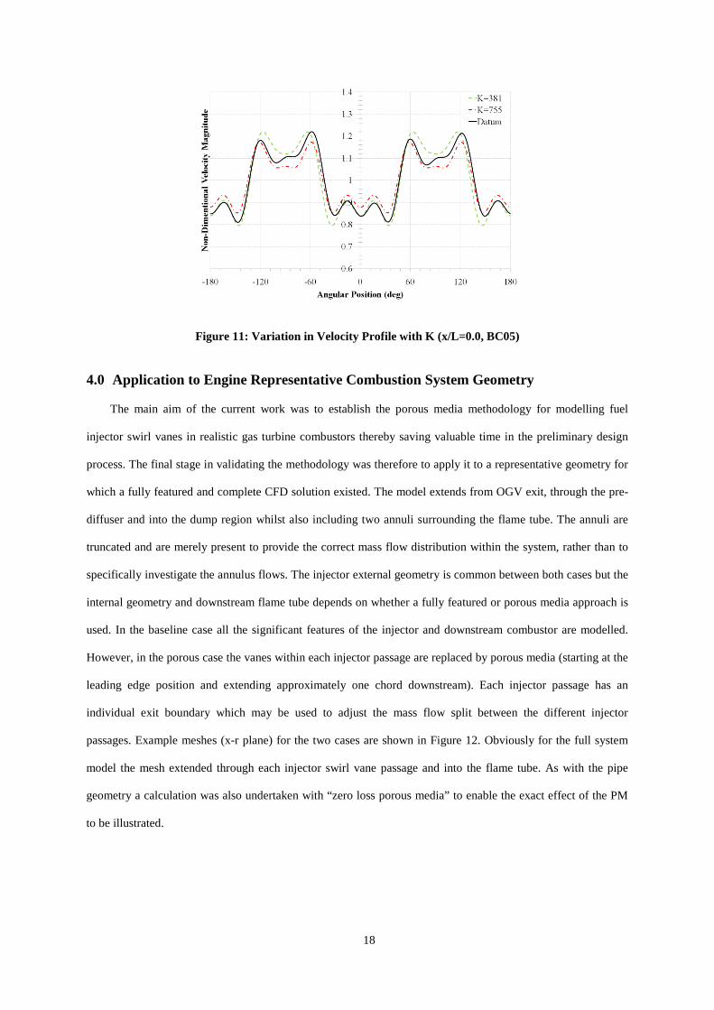
passages. Example meshes (x-r plane) for the two cases are shown in Figure 12. Obviously for the full system

model the mesh extended through each injector swirl vane passage and into the flame tube. As with the pipe

geometry a calculation was also undertaken with “zero loss porous media” to enable the exact effect of the PM

to be illustrated.

19

Figure 12: Centre-Planes of Domain With and Without PM Present

4.1 CFD Methodology

For the porous media case the vanes and downstream combustor geometry were removed and the domain

re-meshed maintaining, where possible, the original mesh density and type. Three meshes were considered, as

detailed in Table 5, covering a range of types and densities. However, comparison of the converged solutions

suggested that similar results were obtained from all three. Mesh 3 was considered to be the most suitable for

comparison since it represents the coarsest mesh and, therefore, gives the largest saving in computational effort.

All future comparisons between the baseline datum case and the porous case are conducted using mesh 3.

Table 5 shows the vast reduction in computational effort achieved via the use of the PM method. The

computational mesh is some 60% smaller than the fully featured geometry and reduces the computation time by

almost 70%. (On a single processor this is equivalent to reducing the computation time from 20 days to almost 5

days). Additionally, there is also a significant saving in the time and effort required to mesh the domain. The

simplicity of the PM case allows the domain to be readily meshed whereas the fully featured geometry requires

significantly more attention in order to generate a good quality mesh. Though this time saving is difficult to

quantify it is significant and should not be overlooked. This is particularly true in the context of a new design or

research project where many geometries may need to be investigated. It is also worthwhile to note the

advantages of smaller solution domains with regard to data storage and post processing which are made easier

by a reduction of cell count.

Throughout all the numerical investigations, a consistent methodology was adopted for all other modelling

aspects. For example in each case a RANS methodology was employed with turbulence closure achieved using

a Realisable k-ε turbulence model in conjunction with standard wall functions. The choice of turbulence model

will obviously influence the solution but the purpose of the current investigation is to compare the effect of the

porous media to a fully featured geometry. Consequently, the influence of the choice of turbulence model was

20

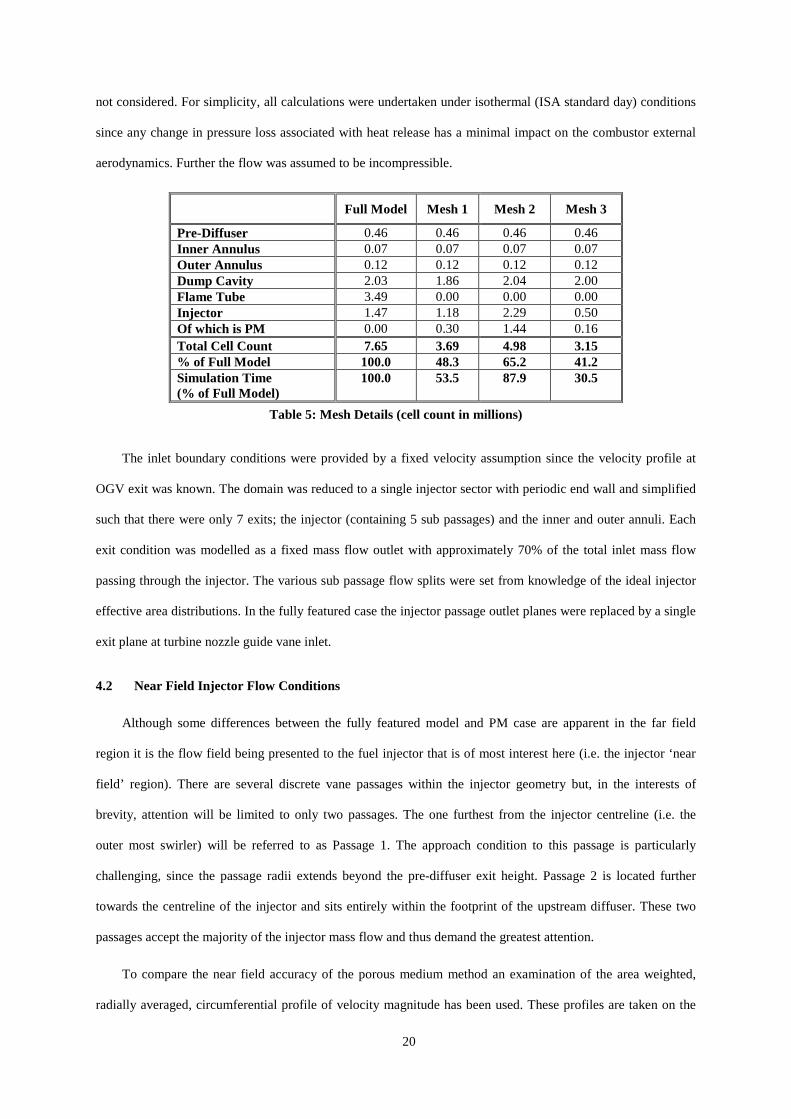
not considered. For simplicity, all calculations were undertaken under isothermal (ISA standard day) conditions

since any change in pressure loss associated with heat release has a minimal impact on the combustor external

aerodynamics. Further the flow was assumed to be incompressible.

Full Model Mesh 1 Mesh 2 Mesh 3

Pre-Diffuser 0.46 0.46 0.46 0.46 Inner Annulus 0.07 0.07 0.07 0.07 Outer Annulus 0.12 0.12 0.12 0.12 Dump Cavity 2.03 1.86 2.04 2.00 Flame Tube 3.49 0.00 0.00 0.00 Injector 1.47 1.18 2.29 0.50 Of which is PM 0.00 0.30 1.44 0.16 Total Cell Count 7.65 3.69 4.98 3.15 % of Full Model 100.0 48.3 65.2 41.2 Simulation Time (% of Full Model)

100.0 53.5 87.9 30.5

Table 5: Mesh Details (cell count in millions)

The inlet boundary conditions were provided by a fixed velocity assumption since the velocity profile at

OGV exit was known. The domain was reduced to a single injector sector with periodic end wall and simplified

such that there were only 7 exits; the injector (containing 5 sub passages) and the inner and outer annuli. Each

exit condition was modelled as a fixed mass flow outlet with approximately 70% of the total inlet mass flow

passing through the injector. The various sub passage flow splits were set from knowledge of the ideal injector

effective area distributions. In the fully featured case the injector passage outlet planes were replaced by a single

exit plane at turbine nozzle guide vane inlet.

4.2 Near Field Injector Flow Conditions

Although some differences between the fully featured model and PM case are apparent in the far field

region it is the flow field being presented to the fuel injector that is of most interest here (i.e. the injector ‘near

field’ region). There are several discrete vane passages within the injector geometry but, in the interests of

brevity, attention will be limited to only two passages. The one furthest from the injector centreline (i.e. the

outer most swirler) will be referred to as Passage 1. The approach condition to this passage is particularly

challenging, since the passage radii extends beyond the pre-diffuser exit height. Passage 2 is located further

towards the centreline of the injector and sits entirely within the footprint of the upstream diffuser. These two

passages accept the majority of the injector mass flow and thus demand the greatest attention.

To compare the near field accuracy of the porous medium method an examination of the area weighted,

radially averaged, circumferential profile of velocity magnitude has been used. These profiles are taken on the

21

PM inlet planes, which are coincident with the location of the swirl vane leading edge for the fully featured case.

Profiles have been Fourrier fitted to a tenth order and are consistent with the methodology described in Section

3. In this way any localised effects caused by the pressure field associated with individual swirl vanes are

removed. Any flow field variations reflect the large scale spatial variations that can be attributed to the external

flow field and the way fluid is being supplied to the injector.

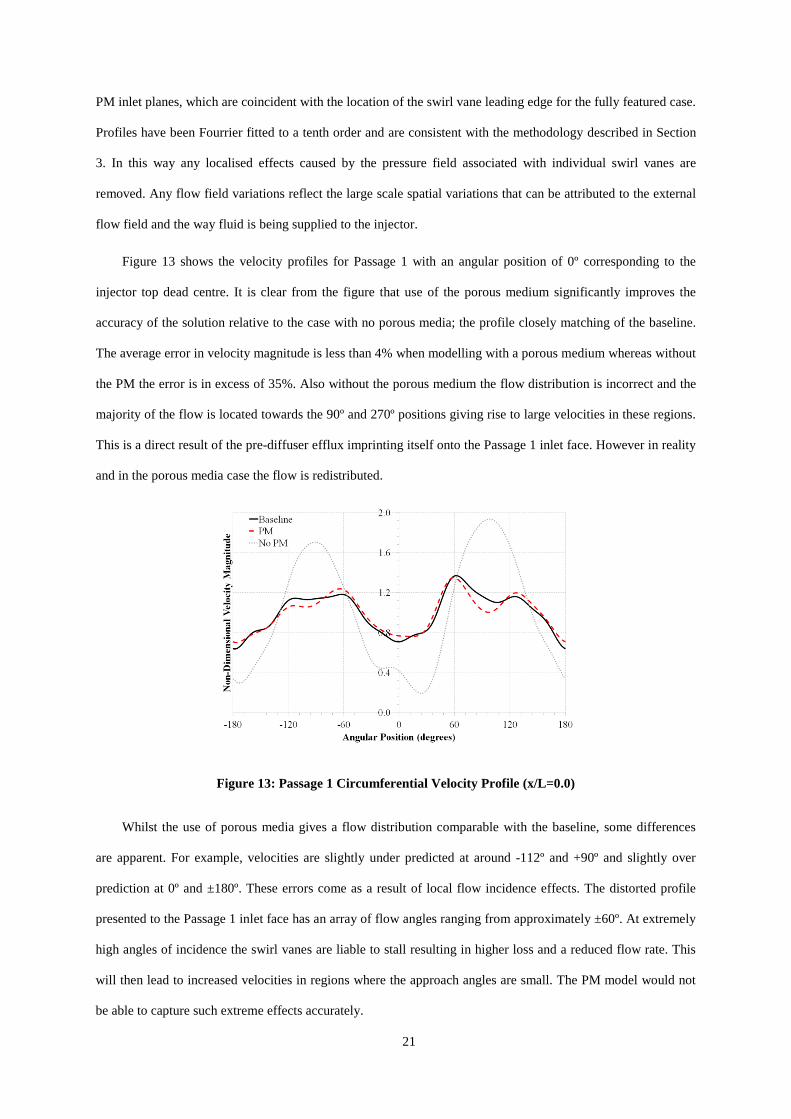
Figure 13 shows the velocity profiles for Passage 1 with an angular position of 0º corresponding to the

injector top dead centre. It is clear from the figure that use of the porous medium significantly improves the

accuracy of the solution relative to the case with no porous media; the profile closely matching of the baseline.

The average error in velocity magnitude is less than 4% when modelling with a porous medium whereas without

the PM the error is in excess of 35%. Also without the porous medium the flow distribution is incorrect and the

majority of the flow is located towards the 90º and 270º positions giving rise to large velocities in these regions.

This is a direct result of the pre-diffuser efflux imprinting itself onto the Passage 1 inlet face. However in reality

and in the porous media case the flow is redistributed.

Figure 13: Passage 1 Circumferential Velocity Profile (x/L=0.0)

Whilst the use of porous media gives a flow distribution comparable with the baseline, some differences

are apparent. For example, velocities are slightly under predicted at around -112º and +90º and slightly over

prediction at 0º and ±180º. These errors come as a result of local flow incidence effects. The distorted profile

presented to the Passage 1 inlet face has an array of flow angles ranging from approximately ±60º. At extremely

high angles of incidence the swirl vanes are liable to stall resulting in higher loss and a reduced flow rate. This

will then lead to increased velocities in regions where the approach angles are small. The PM model would not

be able to capture such extreme effects accurately.

22

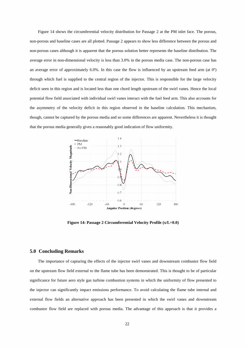
Figure 14 shows the circumferential velocity distribution for Passage 2 at the PM inlet face. The porous,

non-porous and baseline cases are all plotted. Passage 2 appears to show less difference between the porous and

non-porous cases although it is apparent that the porous solution better represents the baseline distribution. The

average error in non-dimensional velocity is less than 3.0% in the porous media case. The non-porous case has

an average error of approximately 6.0%. In this case the flow is influenced by an upstream feed arm (at 0º)

through which fuel is supplied to the central region of the injector. This is responsible for the large velocity

deficit seen in this region and is located less than one chord length upstream of the swirl vanes. Hence the local

potential flow field associated with individual swirl vanes interact with the fuel feed arm. This also accounts for

the asymmetry of the velocity deficit in this region observed in the baseline calculation. This mechanism,

though, cannot be captured by the porous media and so some differences are apparent. Nevertheless it is thought

that the porous media generally gives a reasonably good indication of flow uniformity.

Figure 14: Passage 2 Circumferential Velocity Profile (x/L=0.0)

5.0 Concluding Remarks

The importance of capturing the effects of the injector swirl vanes and downstream combustor flow field

on the upstream flow field external to the flame tube has been demonstrated. This is thought to be of particular

significance for future aero style gas turbine combustion systems in which the uniformity of flow presented to

the injector can significantly impact emissions performance. To avoid calculating the flame tube internal and

external flow fields an alternative approach has been presented in which the swirl vanes and downstream

combustor flow field are replaced with porous media. The advantage of this approach is that it provides a

23

significant reduction in simulation time whilst still enabling the quality of the flow (pressure loss, flow

uniformity) being presented to the injector swirl vanes to be evaluated to a good first order engineering

approximation. The methodology has been shown to be robust, practical and can be achieved through suitable

knowledge of the injector geometry along with the suitable values outlined in this report. Hence this makes the

technique particularly useful during the initial design phase of a project. Once the geometry has been refined a

fully featured calculation may be run and used to define the final geometry safe in the knowledge that the initial

predictions generated using porous media are accurate enough to capture the gross fluid behaviour.

References

[1] Fishenden, C. R. and Stevens, S. J., 1977, “Performance of Annular Combustor Dump Diffusers", Journal

of Aircraft, Vol. 14, pp. 60-67.

[2] Carrotte, J. F., Bailey, D. W. and Frodsham, C. W., 1995, “Detailed Measurements on a Modern

Combustor Dump Diffuser System”, ASME Journal of Engineering for Gas Turbines and Power, Vol. 117,

pp.678-685.

[3] Walker, A. D., Carrotte, J. F. and McGuirk, J. J., 2008, “Compressor/Diffuser/Combustor Aerodynamic

Interactions in Lean Module Combustors”, ASME Journal of Engineering for Gas Turbines and Power,

Vol. 130(1), pp. 011504-1-08.

[4] Barker, A. G. and Carrotte, J. F., 2002, “Compressor Exit Conditions and their Impact on Flame Tube

Injector Flows”, ASME Journal of Engineering for Gas Turbines and Power, Vol. 124(1), pp. 10-19.

[5] Lefebvre, A. H., 1999, “Gas Turbine Combustion”, 2nd Edition, Taylor and Francis.

[6] Lazik, W., Doerr, T. and Bake, S., 2008, “Development of Lean-Burn Low-NOx Combustion Technology

at Rolls-Royce Deutschland”, ASME Paper GT2008-51115.

[7] Walker, A. D., 2002, “Experimental and Computational Study of Hybrid Diffusers for Gas Turbine

Combustors”, PhD Thesis, Dept. Aeronautical and Automotive Engineering, Loughborough University.