The Architecture of Parallel I/O

Rob Lathamrobl@mcs.anl.govMathematics and Computer Science DivisionArgonne National Laboratory

http://www.mcs.anl.gov/~robl/tutorials/csmc/

28 October 2010

Computational Science

Use of computer simulation as a tool for greater understanding of the real world

– Complements experimentation and theory Problems are increasingly computationally

challenging

– Large parallel machines needed to perform calculations

– Critical to leverage parallelism in all phases

Data access is a huge challenge

– Using parallelism to obtain performance

– Finding usable, efficient, portable interfaces

– Understanding and tuning I/O

2

Visualization of entropy in Terascale Supernova Initiative application. Image from Kwan-Liu Ma’s visualization team at UC Davis.

IBM Blue Gene/P system at Argonne National Laboratory.

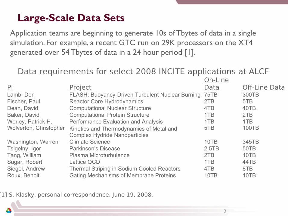
Large-Scale Data SetsApplication teams are beginning to generate 10s of Tbytes of data in a single simulation. For example, a recent GTC run on 29K processors on the XT4 generated over 54 Tbytes of data in a 24 hour period [1].

PI ProjectOn-Line Data Off-Line Data

Lamb, Don FLASH: Buoyancy-Driven Turbulent Nuclear Burning 75TB 300TBFischer, Paul Reactor Core Hydrodynamics 2TB 5TBDean, David Computational Nuclear Structure 4TB 40TBBaker, David Computational Protein Structure 1TB 2TBWorley, Patrick H. Performance Evaluation and Analysis 1TB 1TBWolverton, Christopher Kinetics and Thermodynamics of Metal and

Complex Hydride Nanoparticles5TB 100TB

Washington, Warren Climate Science 10TB 345TBTsigelny, Igor Parkinson's Disease 2.5TB 50TBTang, William Plasma Microturbulence 2TB 10TBSugar, Robert Lattice QCD 1TB 44TBSiegel, Andrew Thermal Striping in Sodium Cooled Reactors 4TB 8TBRoux, Benoit Gating Mechanisms of Membrane Proteins 10TB 10TB

Data requirements for select 2008 INCITE applications at ALCF

[1] S. Klasky, personal correspondence, June 19, 2008.

3

Disk Access Rates over Time

4

Thanks to R. Freitas of IBM Almaden Research Center for providing much of the data for this graph.

5

Applications, Data Models, and I/O Applications have data models

appropriate to domain– Multidimensional typed arrays, images

composed of scan lines, variable length records

– Headers, attributes on data

I/O systems have very simple data models– Tree-based hierarchy of containers– Some containers have streams of bytes

(files)– Others hold collections of other containers

(directories or folders)

Someone has to map from one to the other!

Graphic from J. Tannahill, LLNL

Graphic from A. Siegel, ANL

Challenges in Application I/O

Leveraging aggregate communication and I/O bandwidth of clients– …but not overwhelming a resource limited I/O system with

uncoordinated accesses! Limiting number of files that must be managed

– Also a performance issue Avoiding unnecessary post-processing Often application teams spend so much time on this

that they never get any further:– Interacting with storage through convenient abstractions– Storing in portable formats

Parallel I/O software is available to address all of these problems, when used appropriately.

6

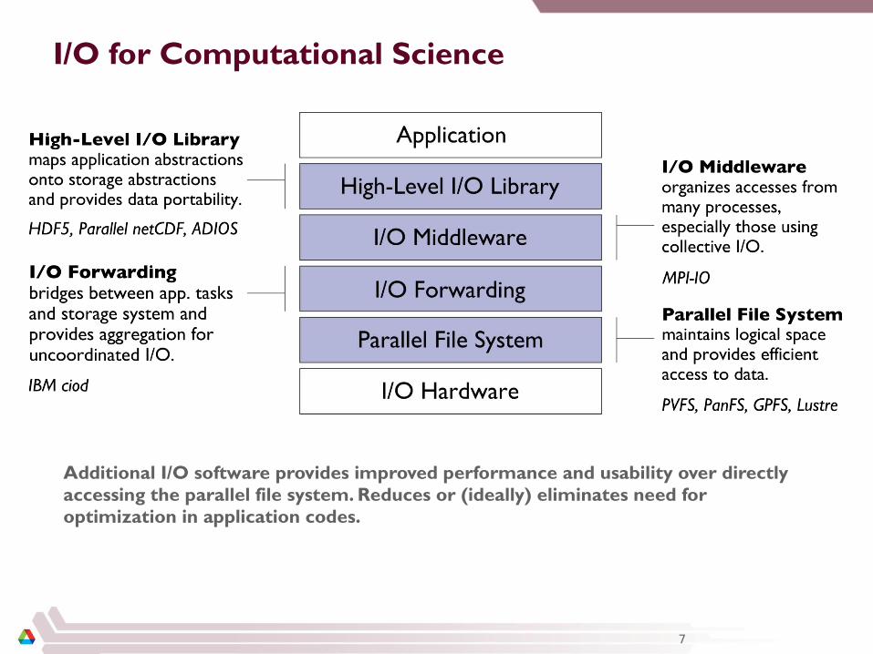
I/O for Computational Science

Additional I/O software provides improved performance and usability over directly accessing the parallel file system. Reduces or (ideally) eliminates need for optimization in application codes.

7

The Present: Oak Ridge Computing Platform

Figure compliments Galen Shipman (ORNL), Feb. 16, 2010. 8

I/O Hardware and Software on Blue Gene/P

9

High-level Libraries and MPI-IO Software

10

I/O Forwarding Software

11

Parallel File SystemSoftware

12

Exascale Systems: Potential ArchitectureSystems 2009 2018 Differenc

e

System Peak 2 Pflop/sec 1 Eflop/sec O(1000)

Power 6 Mwatt 20 Mwatt

System Memory 0.3 Pbytes 32-64 Pbytes O(100)

Node Compute 125 Gflop/sec 1-15 Tflop/sec O(10-100)

Node Memory BW 25 Gbytes/sec 2-4 Tbytes/sec O(100)

Node Concurrency 12 O(1-10K) O(100-1000)

Total Node Interconnect BW 3.5 Gbytes/sec 200-400 Gbytes/sec O(100)

System Size (Nodes) 18,700 O(100,000-1M) O(10-100)

Total Concurrency 225,000 O(1 billion) O(10,000)

Storage 15 Pbytes 500-1000 Pbytes O(10-100)

I/O 0.2 Tbytes/sec 60 Tbytes/sec O(100)

MTTI Days O(1 day)

From J. Dongarra, “Impact of Architecture and Technology for Extreme Scale on Software and Algorithm Design,” Cross-cutting Technologies for Computing at the Exascale, February 2-5, 2010. 13

The MPI-IO Interface

14

15

MPI-IO

I/O interface specification for use in MPI apps Data model is same as POSIX

– Stream of bytes in a file

Features:– Collective I/O– Noncontiguous I/O with MPI datatypes and file views– Nonblocking I/O– Fortran bindings (and additional languages)– System for encoding files in a portable format (external32)

• Not self-describing - just a well-defined encoding of types

Implementations available on most platforms (more later)

16

Independent and Collective I/O

Independent I/O operations specify only what a single process will do– Independent I/O calls do not pass on relationships between I/O on other processes

Many applications have phases of computation and I/O– During I/O phases, all processes read/write data

– We can say they are collectively accessing storage

Collective I/O is coordinated access to storage by a group of processes– Collective I/O functions are called by all processes participating in I/O– Allows I/O layers to know more about access as a whole, more opportunities for

optimization in lower software layers, better performance

P0 P1 P2 P3 P4 P5 P0 P1 P2 P3 P4 P5

Independent I/O Collective I/O

17

Process 0 Process 0 Process 0Process 0

Contiguous Noncontiguousin File

Noncontiguousin Memory

Noncontiguousin Both

Contiguous and Noncontiguous I/O

Contiguous I/O moves data from a single memory block into a single file region

Noncontiguous I/O has three forms:

– Noncontiguous in memory, noncontiguous in file, or noncontiguous in both

Structured data leads naturally to noncontiguous I/O (e.g. block decomposition)

Describing noncontiguous accesses with a single operation passes more knowledge to I/O system

18

Nonblocking and Asynchronous I/O

Blocking, or Synchronous, I/O operations return when buffer may be reused– Data in system buffers or on disk

Some applications like to overlap I/O and computation– Hiding writes, prefetching, pipelining

A nonblocking interface allows for submitting I/O operations and testing for completion later

If the system also supports asynchronous I/O, progress on operations can occur in the background– Depends on implementation

Otherwise progress is made at start, test, wait calls

Noncontiguous I/O: Data Sieving

Data sieving is used to combine lots of small accesses into a single larger one– Remote file systems (parallel or

not) tend to have high latencies

– Reducing # of operations important

Similar to how a block-based file system interacts with storage

Generally very effective, but not as good as having a PFS that supports noncontiguous access

Buffer

Memory

File

Data Sieving Read Transfers

19

Data Sieving Write Operations

Buffer

Memory

File

Data Sieving Write Transfers

Data sieving for writes is more complicated– Must read the entire region first– Then make changes in buffer– Then write the block back

Requires locking in the file system– Can result in false sharing

(interleaved access)

PFS supporting noncontiguous writes is preferred

20

21

Collective I/O and Two-Phase I/O

Problems with independent, noncontiguous access– Lots of small accesses– Independent data sieving reads lots of extra data, can exhibit false sharing

Idea: Reorganize access to match layout on disks– Single processes use data sieving to get data for many– Often reduces total I/O through sharing of common blocks

Second “phase” redistributes data to final destinations Two-phase writes operate in reverse (redistribute then I/O)

– Typically read/modify/write (like data sieving)

– Overhead is lower than independent access because there is little or no false sharing

Note that two-phase is usually applied to file regions, not to actual blocks

Two-Phase Read Algorithm

p0 p1 p2 p0 p1 p2 p0 p1 p2

Phase 1: I/OInitial State Phase 2: Redistribution

Two-Phase I/O Algorithms

22

For more information, see W.K. Liao and A. Choudhary, “Dynamically Adapting File Domain Partitioning Methods for Collective I/O Based on Underlying Parallel File System Locking Protocols,” SC2008, November, 2008.

Impact of Two-Phase I/O Algorithms

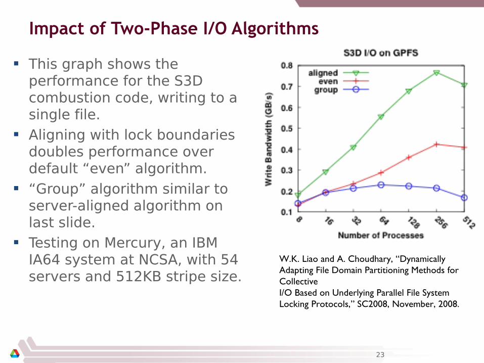
This graph shows the performance for the S3D combustion code, writing to a single file.

Aligning with lock boundaries doubles performance over default “even” algorithm.

“Group” algorithm similar to server-aligned algorithm on last slide.

Testing on Mercury, an IBM IA64 system at NCSA, with 54 servers and 512KB stripe size.

23

W.K. Liao and A. Choudhary, “Dynamically Adapting File Domain Partitioning Methods for Collective I/O Based on Underlying Parallel File System Locking Protocols,” SC2008, November, 2008.

S3D Turbulent Combustion Code

S3D is a turbulent combustion application using a direct numerical simulation solver from Sandia National Laboratory

Checkpoints consist of four global arrays– 2 3-dimensional– 2 4-dimensional– 50x50x50 fixed

subarrays

24

Thanks to Jackie Chen (SNL), Ray Grout (SNL), and Wei-Keng Liao (NWU) for providing the S3D I/O benchmark, Wei-Keng Liao for providing this diagram.

Impact of Optimizations on S3D I/O Testing with PnetCDF output to single file, three configurations,

16 processes– All MPI-IO optimizations (collective buffering and data sieving)

disabled– Independent I/O optimization (data sieving) enabled– Collective I/O optimization (collective buffering, a.k.a. two-phase

I/O) enabled

25

Coll. Buffering and Data Sieving Disabled

Data Sieving Enabled

Coll. Buffering Enabled (incl. Aggregation)

POSIX writes 102,401 81 5

POSIX reads 0 80 0

MPI-IO writes 64 64 64

Unaligned in file 102,399 80 4

Total written (MB) 6.25 87.11 6.25

Runtime (sec) 1443 11 6.0

Avg. MPI-IO time per proc (sec)

1426.47 4.82 0.60

26

Common FunctionalityADIO Interface

UFS

MPI-IO Interface

NFS XFSPVFSROMIO’s layered architecture.

MPI-IO Implementations

Different MPI-IO implementations exist Three better-known ones are:

– ROMIO from Argonne National Laboratory• Leverages MPI-1 communication• Supports local file systems, network file systems,

parallel file systems– UFS module works GPFS, Lustre, and others

• Includes data sieving and two-phase optimizations– MPI-IO/GPFS from IBM (for AIX only)

• Includes two special optimizations– Data shipping -- mechanism for coordinating access to a file to alleviate

lock contention (type of aggregation)– Controlled prefetching -- using MPI file views and access patterns to

predict regions to be accessed in future

– MPI from NEC• For NEC SX platform and PC clusters with Myrinet, Quadrics,

IB, or TCP/IP• Includes listless I/O optimization -- fast handling of

noncontiguous I/O accesses in MPI layer

The Parallel netCDF Interface and File Format

27

Thanks to Wei-Keng Liao, Alok Choudhary, and Kui Gao (NWU) for their help in the development of PnetCDF.

Higher Level I/O Interfaces

Provide structure to files– Well-defined, portable formats– Self-describing– Organization of data in file– Interfaces for discovering contents

Present APIs more appropriate for computational science– Typed data– Noncontiguous regions in memory and file– Multidimensional arrays and I/O on subsets of these arrays

Both of our example interfaces are implemented on top of MPI-IO

28

Parallel netCDF (PnetCDF)

Based on original “Network Common Data Format” (netCDF) work from Unidata

– Derived from their source code

Data Model:

– Collection of variables in single file

– Typed, multidimensional array variables

– Attributes on file and variables

Features:

– C and Fortran interfaces

– Portable data format (identical to netCDF)

– Noncontiguous I/O in memory using MPI datatypes

– Noncontiguous I/O in file using sub-arrays

– Collective I/O

– Non-blocking I/O

Unrelated to netCDF-4 work

29

Data Layout in netCDF Files

30

Record Variables in netCDF

Record variables are defined to have a single “unlimited” dimension– Convenient when a dimension size is

unknown at time of variable creation

Record variables are stored after all the other variables in an interleaved format– Using more than one in a file is likely to

result in poor performance due to number of noncontiguous accesses

31

Storing Data in PnetCDF

Create a dataset (file)– Puts dataset in define mode– Allows us to describe the contents

• Define dimensions for variables• Define variables using dimensions• Store attributes if desired (for variable or dataset)

Switch from define mode to data mode to write variables Store variable data Close the dataset

32

Example: FLASH Astrophysics

FLASH is an astrophysics code forstudying events such as supernovae– Adaptive-mesh hydrodynamics

– Scales to 1000s of processors

– MPI for communication

Frequently checkpoints:– Large blocks of typed variables

from all processes

– Portable format

– Canonical ordering (different thanin memory)

– Skipping ghost cells

33

Ghost cell

Stored element

…Vars 0, 1, 2, 3, … 23

Example: FLASH with PnetCDF

FLASH AMR structures do not map directly to netCDF multidimensional arrays

Must create mapping of the in-memory FLASH data structures into a representation in netCDF multidimensional arrays

Chose to– Place all checkpoint data in a single file– Impose a linear ordering on the AMR blocks

• Use 4D variables

– Store each FLASH variable in its own netCDF variable• Skip ghost cells

– Record attributes describing run time, total blocks, etc.

34

Defining Dimensions

int status, ncid, dim_tot_blks, dim_nxb,dim_nyb, dim_nzb;

MPI_Info hints;/* create dataset (file) */status = ncmpi_create(MPI_COMM_WORLD, filename,

NC_CLOBBER, hints, &file_id);/* define dimensions */status = ncmpi_def_dim(ncid, "dim_tot_blks",

tot_blks, &dim_tot_blks);status = ncmpi_def_dim(ncid, "dim_nxb",

nzones_block[0], &dim_nxb);status = ncmpi_def_dim(ncid, "dim_nyb",

nzones_block[1], &dim_nyb);status = ncmpi_def_dim(ncid, "dim_nzb",

nzones_block[2], &dim_nzb);

35

Each dimension getsa unique reference

Creating Variables

int dims = 4, dimids[4];int varids[NVARS];/* define variables (X changes most quickly) */dimids[0] = dim_tot_blks;dimids[1] = dim_nzb;dimids[2] = dim_nyb;dimids[3] = dim_nxb;for (i=0; i < NVARS; i++) {

status = ncmpi_def_var(ncid, unk_label[i],NC_DOUBLE, dims, dimids, &varids[i]);

}

36

Same dimensions usedfor all variables

Storing Attributes

/* store attributes of checkpoint */status = ncmpi_put_att_text(ncid, NC_GLOBAL,

"file_creation_time", string_size, file_creation_time);status = ncmpi_put_att_int(ncid, NC_GLOBAL, "total_blocks",

NC_INT, 1, tot_blks);status = ncmpi_enddef(file_id);

/* now in data mode … */

37

Writing Variables

double *unknowns; /* unknowns[blk][nzb][nyb][nxb] */size_t start_4d[4], count_4d[4];start_4d[0] = global_offset; /* different for each process */start_4d[1] = start_4d[2] = start_4d[3] = 0;count_4d[0] = local_blocks;count_4d[1] = nzb; count_4d[2] = nyb; count_4d[3] = nxb;for (i=0; i < NVARS; i++) {

/* ... build datatype “mpi_type” describing values of a single variable ... */

/* collectively write out all values of a single variable */ncmpi_put_vara_all(ncid, varids[i], start_4d, count_4d,

unknowns, 1, mpi_type);}status = ncmpi_close(file_id);

38

Typical MPI buffer-count-type tuple

Inside PnetCDF Define Mode

In define mode (collective)– Use MPI_File_open to create file at create time– Set hints as appropriate (more later)– Locally cache header information in memory

• All changes are made to local copies at each process

At ncmpi_enddef – Process 0 writes header with MPI_File_write_at – MPI_Bcast result to others– Everyone has header data in memory, understands placement of all

variables• No need for any additional header I/O during data mode!

39

Inside PnetCDF Data Mode

Inside ncmpi_put_vara_all (once per variable) – Each process performs data conversion into internal buffer– Uses MPI_File_set_view to define file region

• Contiguous region for each process in FLASH case

– MPI_File_write_all collectively writes data

At ncmpi_close – MPI_File_close ensures data is written to storage

MPI-IO performs optimizations– Two-phase possibly applied when writing variables

MPI-IO makes PFS calls– PFS client code communicates with servers and stores data

40

Inside Parallel netCDF: Jumpshot view

41

1: Rank 0 write header(independent I/O)

2: Collectively writeapp grid, AMR data

3: Collectively write 4 variables

4: Close file

I/O Aggregator

PnetCDF Wrap-Up

PnetCDF gives us– Simple, portable, self-describing container for data– Collective I/O– Data structures closely mapping to the variables described

If PnetCDF meets application needs, it is likely to give good performance– Type conversion to portable format does add overhead

Some limits on (old, common CDF-2) file format:– Fixed-size variable: < 4 GiB– Per-record size of record variable: < 4 GiB– 232 -1 records – New extended file format to relax these limits (CDF-5, released in

pnetcdf-1.1.0)

42

The HDF5 Interface and File Format

43

HDF5

Hierarchical Data Format, from the HDF Group (formerly of NCSA) Data Model:

– Hierarchical data organization in single file– Typed, multidimensional array storage– Attributes on dataset, data

Features:– C, C++, and Fortran interfaces– Portable data format– Optional compression (not in parallel I/O mode)– Data reordering (chunking)– Noncontiguous I/O (memory and file) with hyperslabs

44

HDF5 Files

HDF5 files consist of groups, datasets, and attributes– Groups are like directories, holding other groups and datasets– Datasets hold an array of typed data

• A datatype describes the type (not an MPI datatype)• A dataspace gives the dimensions of the array

– Attributes are small datasets associated with the file, a group, or another dataset

• Also have a datatype and dataspace• May only be accessed as a unit

45

Dataset “temp”

HDF5 File “chkpt007.h5”

Group “/”

Group “viz”datatype = H5T_NATIVE_DOUBLEdataspace = (10, 20)

attributes = …

10 (data)

20

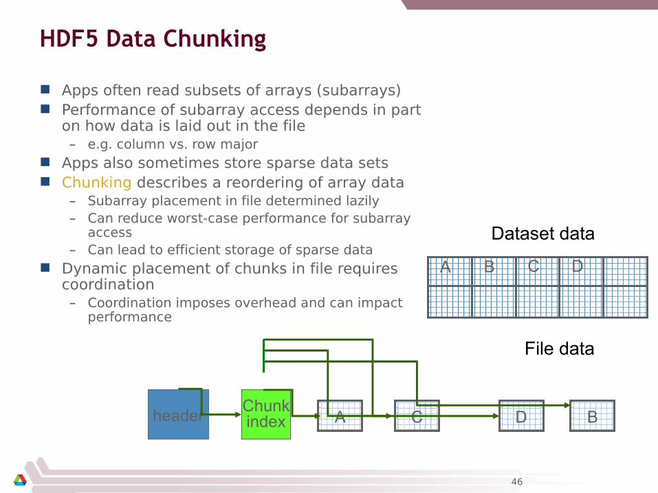
HDF5 Data Chunking

Apps often read subsets of arrays (subarrays) Performance of subarray access depends in part

on how data is laid out in the file– e.g. column vs. row major

Apps also sometimes store sparse data sets Chunking describes a reordering of array data

– Subarray placement in file determined lazily– Can reduce worst-case performance for subarray

access– Can lead to efficient storage of sparse data

Dynamic placement of chunks in file requires coordination– Coordination imposes overhead and can impact

performance

46

Dataset data

A B C D

A DC BheaderChunkindex

File data

Example: FLASH Particle I/O with HDF5

FLASH “Lagrangian particles” record location, characteristics of reaction

– Passive particles don’t exert forces; pushed along but do not interact

Particle data included in checkpoints, but not in plotfiles; dump particle data to separate file

One particle dump file per time step

– i.e., all processes write to single particle file

Output includes application info, runtime info in addition to particle data

47

Block=30;Pos_x=0.65;Pos_y=0.35;Pos_z=0.125;Tag=65;Vel_x=0.0;Vel_y=0.0;vel_z=0.0;

Typical particle data

Opening file

hid_t acc_template;ierr = H5Pset_alignment(acc_template, 524288, 262144);ierr = MPI_Info_set(info, "IBM_largeblock_io", "true");

/* set the file access template for parallel IO */ac_template = H5Pcreate(H5P_FILE_ACCESS);/* tell HDF5 to use MPI-IO interface */ierr = H5Pset_fapl_mpio(acc_template, *io_comm, info);

/* create the file collectively */file_identifier = H5Fcreate(filename, H5F_ACC_TRUNC, H5P_DEFAULT, acc_template);/* release the file access template */ierr = H5Pclose(acc_template);

48

“P”: property list“F”: file operations“S”: dataspace,“T”: datatype,“D”: dataset!

Storing Labels for Particles

int string_size = OUTPUT_PROP_LENGTH;hsize_t dims_2d[2] = {npart_props, 1};hid_t dataspace, dataset, file_id, string_type;

/* store string creation time attribute */string_type = H5Tcopy(H5T_C_S1);H5Tset_size(string_type, string_size);dataspace = H5Screate_simple(2, dims_2d, NULL);dataset = H5Dcreate(file_id, “particle names", string_type,

dataspace, H5P_DEFAULT);if (myrank == 0) {

status = H5Dwrite(dataset, string_type, H5S_ALL, H5S_ALL, H5P_DEFAULT, particle_labels);

}

49

get a copy of thestring type and

resize it

Write out all 8 labels in one call

Remember:“S” is for dataspace,“T” is for datatype,“D” is for dataset!

Storing Particle Data with Hyperslabs (1 of 2)

hsize_t dims_2d[2];

/* Step 1: set up dataspace – describe global layout */

dims_2d[0] = total_particles;dims_2d[1] = npart_props;

dspace = H5Screate_simple(2, dims_2d, NULL);dset = H5Dcreate(file_id, “tracer particles”,

H5T_NATIVE_DOUBLE, dspace, H5P_DEFAULT);

50

Remember:“S” is for dataspace,“T” is for datatype,“D” is for dataset!

local_np = 2, part_offset = 3, total_particles = 10,Npart_props = 8

Storing Particle Data with Hyperslabs (2 of 2)

hsize_t start_2d[2] = {0, 0}, stride_2d[1] = {1, 1};hsize_t count_2d[2] = {local_np, npart_props};

/* Step 2: setup hyperslab for dataset in file */

start_2d[0] = part_offset; /* MPI_Allgather earlier determined particles */status = H5Sselect_hyperslab(dspace, H5S_SELECT_SET, start_2d, stride_2d, count_2d, NULL);

51

dataspace fromlast slide

local_np = 2, part_offset = 3, total_particles = 10,Npart_props = 8

- Hyperslab selection similar to MPI-IO file view- Selections don’t overlap in this example (would be bad if writing!)- H5SSelect_none() if no work for this process

Collectively Writing Particle Data

/* Step 1: specify collective I/O */dxfer_plist = H5Pcreate(H5P_DATASET_XFER);Ierr = H5Pset_dxpl_mpio(dxfer_plist,

H5FD_MPIO_COLLECTIVE);

/* Step 2: perform collective write */status = H5Dwrite(dataset,

H5T_NATIVE_DOUBLE, memspace, dspace, dxfer_plist , particles);

52

“P” is for property list;tuning parameters

dataspace describing memory,

could also use a hyperslab

dataspace describing region in file, with

hyperslab from previous two slides

Remember:“S” is for dataspace,“T” is for datatype,“D” is for dataset!

Inside HDF5

MPI_File_open used to open file Because there is no “define” mode, file layout is

determined at write time In H5Dwrite:

– Processes communicate to determine file layout• Process 0 performs metadata updates after write

– Call MPI_File_set_view– Call MPI_File_write_all to collectively write

• Only if enabled via property list Memory hyperslab could have been used to define

noncontiguous region in memory In FLASH application, data is kept in native format

and converted at read time (defers overhead)– Could store in some other format if desired

At the MPI-IO layer:– Metadata updates at every write are a bit of a bottleneck

• MPI-IO from process 0 introduces some skew

53

Inside HDF5: Jumpshot view

54

1: Rank 0 write initial structure(multiple independent I/O)

3: Determine location For variable (orange)

5: Rank 0 writes final md

6: Close file2: Collectively write grid, provenance data

4: Collectively write variable (blue)

HDF5 Wrap-up

Tremendous flexibility: 300+ routines H5Lite high level routines for common cases Tuning via property lists

– “use MPI-IO to access this file”– “read this data collectively”

Extensive on-line documentation, tutorials (see “On Line Resources” slide)

New efforts: – Journaling: make datasets more robust in face of crashes (Sandia)– Fast appends (finance motivated)– Single-writer, Multiple-reader semantics– Aligning data structures to underlying file system

55

Other High-Level I/O libraries

NetCDF-4: http://www.unidata.ucar.edu/software/netcdf/netcdf-4/– netCDF API with HDF5 back-end

ADIOS: http://adiosapi.org– Configurable (xml) I/O approaches

SILO: https://wci.llnl.gov/codes/silo/– A mesh and field library on top of HDF5 (and others)

H5part: http://vis.lbl.gov/Research/AcceleratorSAPP/– simplified HDF5 API for particle simulations

GIO: https://svn.pnl.gov/gcrm– Targeting geodesic grids as part of GCRM

PIO:– climate-oriented I/O library; supports raw binary, parallel-netcdf, or

serial-netcdf (from master)

… Many more: my point: it's ok to make your own.

I/O in Parallel Volume Rendering

Thanks to Tom Peterka (ANL) and Hongfeng Yu and Kwan-Liu Ma (UC Davis) for providing the code on which this material is based.

57

58

Parallel Volume Rendering

Supernova model with focuson core collapse

Parallel rendering techniquesscale to 16k cores on ArgonneBlue Gene/P

Produce a series of time steps 11203 elements (~1.4 billion) Structured grid Simulated and rendered on

multiple platforms, sites I/O time now largest

component of runtime

# of Cores

59

The I/O Code (essentially): MPI_Init(&argc, &argv); ncmpi_open(MPI_COMM_WORLD, argv[1], NC_NOWRITE, info, &ncid)); ncmpi_inq_varid(ncid, argv[2], &varid); buffer =calloc(sizes[0]*sizes[1]*sizes[2],sizeof(float)); for (i=0; i<blocks; i++) { decompose(rank, nprocs, ndims, dims, starts, sizes); ncmpi_get_vara_float_all(ncid, varid, starts, sizes, buffer); } ncmpi_close(ncid)); MPI_Finalize();

Read-only workload: no switch between define/data mode Omits error checking, full use of inquire (ncmpi_inq_*) routines Collective I/O of noncontiguous (in file) data “black box” decompose function:

– divide 1120^3 elements into roughly equal mini-cubes– “face-wise” decomposition ideal for I/O access, but poor fit for

volume rendering algorithms

60

Volume Rendering and pNetCDF

Original data: netCDF formatted Two approaches for I/O

– Pre-processing: extract each variable to separate file• Lengthy, duplicates data

– Native: read data in parallel, on-demand from dataset• Skip preprocessing step but slower than raw

Why so slow?– 5 large “record” variables in

a single netcdf file• Interleaved on per-record basis

– Bad interaction with defaultMPI-IO parameters

Record variable interleaving is performed in N-1 dimension slices, where N is the number of dimensions in the variable.

61

Access Method Comparison

MPI-IO hints matter HDF5: many small

metadatareads

Interleaved record format: bad news

API time (s) accesses read data (MB) efficency

MPI (raw data) 11.388 960 7126 75.20%

PnetCDF (no hints) 36.030 1863 24200 22.15%

PnetCDF (hints) 18.946 2178 7848 68.29%

HDF5 16.862 23450 7270 73.72%

PnetCDF (beta) 13.128 923 7262 73.79%

62

Analysis: Parallel netCDF, no hints

Block depiction of 28 GB file Record variable scattered Reading in way too much

data!

Default “cb_buffer_size” hint not good for interleaved netCDF record variables

offse

ttime

63

With tuning, much less reading

Better efficiency, but still short of MPI-IO

Still some overlap “cb_buffer_size” now size of

one netCDF record Better efficiency, at slight

perf cost

offse

ttime

Analysis: Parallel netCDF, hints

64

Analysis: Parallel HDF5

Different file format, different characteristics

Data exhibits spatial locality

Thousands of metadata reads

– All clients read MD from file

Reads could be batched. Not sure why not (implementation detail: HDF5 folks on the case).

offse

ttime

65

Analysis: new Parallel netCDF

Development effort to relax netCDF file format limits

No need for record variables Data nice and compact like

MPI-IO and HDF5

Rank 0 reads header, broadcasts to others

– Much more scalable approach

Approaching MPI-IO efficiency

Maintains netCDF benefits

– Portable, self-describing, etc.

offse

ttime

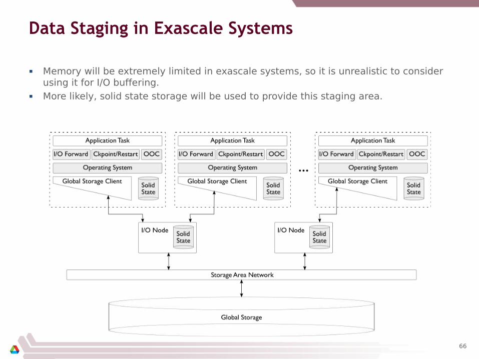
Data Staging in Exascale Systems

Memory will be extremely limited in exascale systems, so it is unrealistic to consider using it for I/O buffering.

More likely, solid state storage will be used to provide this staging area.

66

Data Analysis Options

In situ – process the data (to some degree) in the context of the running application

Co-processing – process the data around the same time as the simulation is run, but not on the simulation nodes

Post-processing – store the data and process it later

Image compliments V. Vishwanath (ANL).

Current system architectures integrate a separate analysis cluster that shares access to storage over a large switch complex. Most data analysis is performed after simulations are complete (post-processed) on these nodes, or processed remotely.

67

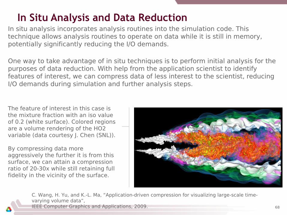
In Situ Analysis and Data ReductionIn situ analysis incorporates analysis routines into the simulation code. This technique allows analysis routines to operate on data while it is still in memory, potentially significantly reducing the I/O demands.

One way to take advantage of in situ techniques is to perform initial analysis for the purposes of data reduction. With help from the application scientist to identify features of interest, we can compress data of less interest to the scientist, reducing I/O demands during simulation and further analysis steps.

The feature of interest in this case is the mixture fraction with an iso value of 0.2 (white surface). Colored regions are a volume rendering of the HO2 variable (data courtesy J. Chen (SNL)).

By compressing data more aggressively the further it is from this surface, we can attain a compression ratio of 20-30x while still retaining full fidelity in the vicinity of the surface.

C. Wang, H. Yu, and K.-L. Ma, “Application-driven compression for visualizing large-scale time-varying volume data”,IEEE Computer Graphics and Applications, 2009. 68

Merging Analysis and Storage Resources

One way to reduce costs, and to potentially improve post-processing rates, is to merge analysis resources with storage resources. Need to move to using commodity storage (if possible) at the same time.

69

70

Printed References

John May, Parallel I/O for High Performance Computing, Morgan Kaufmann, October 9, 2000.– Good coverage of basic concepts, some MPI-IO, HDF5, and

serial netCDF– Out of print?

William Gropp, Ewing Lusk, and Rajeev Thakur, Using MPI-2: Advanced Features of the Message Passing Interface, MIT Press, November 26, 1999.– In-depth coverage of MPI-IO API, including a very detailed

description of the MPI-IO consistency semantics

71

On-Line References

netCDF and netCDF-4– http://www.unidata.ucar.edu/packages/netcdf/

PnetCDF– http://www.mcs.anl.gov/parallel-netcdf/

ROMIO MPI-IO– http://www.mcs.anl.gov/romio/

HDF5 and HDF5 Tutorial– http://www.hdfgroup.org/

– http://hdf.ncsa.uiuc.edu/HDF5/

– http://hdf.ncsa.uiuc.edu/HDF5/doc/Tutor/index.html

POSIX I/O Extensions– http://www.opengroup.org/platform/hecewg/

Darshan I/O Characterization Tool– http://www.mcs.anl.gov/research/projects/darshan