The Atmospheric Bridge: The Inﬂuence of ENSO ... · 15 AUGUST 2002 ALEXANDER ET AL. 2205 q 2002...

15 AUGUST 2002 2205A L E X A N D E R E T A L .

q 2002 American Meteorological Society

The Atmospheric Bridge: The Influence of ENSO Teleconnections on Air–SeaInteraction over the Global Oceans

MICHAEL A. ALEXANDER

NOAA–CIRES Climate Diagnostics Center, Boulder, Colorado

ILEANA BLADE

Laboratori d’Enginyeria Maritima, Universitat Politecnica de Catalunya, Barcelona, Spain

MATTHEW NEWMAN


JOHN R. LANZANTE AND NGAR-CHEUNG LAU

NOAA/Geophysical Fluid Dynamics Laboratory, Princeton, New Jersey

JAMES D. SCOTT


(Manuscript received 31 July 2001, in final form 1 March 2002)

ABSTRACT

During El Nino–Southern Oscillation (ENSO) events, the atmospheric response to sea surface temperature(SST) anomalies in the equatorial Pacific influences ocean conditions over the remainder of the globe. Thisconnection between ocean basins via the ‘‘atmospheric bridge’’ is reviewed through an examination of previouswork augmented by analyses of 50 years of data from the National Centers for Environmental Prediction–National Center for Atmospheric Research (NCEP–NCAR) reanalysis project and coupled atmospheric generalcirculation (AGCM)–mixed layer ocean model experiments. Observational and modeling studies have nowestablished a clear link between SST anomalies in the equatorial Pacific with those in the North Pacific, northtropical Atlantic, and Indian Oceans in boreal winter and spring. ENSO-related SST anomalies also appear tobe robust in the western North Pacific during summer and in the Indian Ocean during fall. While surface heatfluxes are the key component of the atmospheric bridge driving SST anomalies, Ekman transport also createsSST anomalies in the central North Pacific although the full extent of its impact requires further study. Theatmospheric bridge not only influences SSTs on interannual timescales but also affects mixed layer depth (MLD),salinity, the seasonal evolution of upper-ocean temperatures, and North Pacific SST variability at lower fre-quencies. The model results indicate that a significant fraction of the dominant pattern of low-frequency (.10yr) SST variability in the North Pacific is associated with tropical forcing. AGCM experiments suggest that theoceanic feedback on the extratropical response to ENSO is complex, but of modest amplitude. Atmosphere–ocean coupling outside of the tropical Pacific slightly modifies the atmospheric circulation anomalies in thePacific–North America (PNA) region but these modifications appear to depend on the seasonal cycle and air–sea interactions both within and beyond the North Pacific Ocean.

1. Introduction

While air–sea interactions responsible for El Nino andthe Southern Oscillation (ENSO) are centered in theequatorial Pacific Ocean, changes in tropical convectionassociated with ENSO influence the global atmosphericcirculation. The ENSO-driven large-scale atmospheric

Corresponding author address: Michael Alexander, NOAA–CI-RES Climate Diagnostics Center, R/CDC1, 325 Broadway, Boulder,CO 80305-3328.E-mail: [email protected]

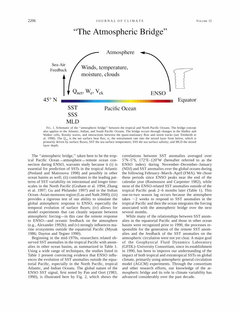
teleconnections alter the near-surface air temperature,humidity, and wind, as well as the distribution of cloudsfar from the equatorial Pacific. The resulting variationsin the surface heat, momentum, and freshwater fluxescan induce changes in sea surface temperature (SST),salinity, mixed layer depth (MLD), and ocean currents.Thus, the atmosphere acts as a bridge spanning fromthe equatorial Pacific to the North Pacific, illustrated inFig. 1, and to the South Pacific, the Atlantic, and IndianOceans. The ENSO-related SST anomalies that developover the world’s oceans can also feed back on the orig-inal atmospheric response to ENSO.

2206 VOLUME 15J O U R N A L O F C L I M A T E

FIG. 1. Schematic of the ‘‘atmospheric bridge’’ between the tropical and North Pacific Oceans. The bridge conceptalso applies to the Atlantic, Indian, and South Pacific Oceans. The bridge occurs through changes in the Hadley andWalker cells, Rossby waves, and interactions between the quasi-stationary flow and storm tracks (see Trenberth etal. 1998). The Qnet is the net surface heat flux; we the entrainment rate into the mixed layer from below, which isprimarily driven by surface fluxes; SST the sea surface temperature; SSS the sea surface salinity; and MLD the mixedlayer depth.

The ‘‘atmospheric bridge,’’ taken here to be the trop-ical Pacific Ocean→atmosphere↔remote ocean con-nection during ENSO, warrants study because it (i) isessential for prediction of SSTs in the tropical Atlantic(Penland and Matrosova 1998) and possibly in otherocean basins as well; (ii) contributes to the leading pat-terns of SST variability on interannual and longer time-scales in the North Pacific (Graham et al. 1994; Zhanget al. 1997; Gu and Philander 1997) and in the IndianOcean–Asian monsoon region (Lau and Nath 2000); (iii)provides a rigorous test of our ability to simulate theglobal atmospheric response to ENSO, especially thetemporal evolution of surface fluxes; (iv) allows formodel experiments that can cleanly separate betweenatmospheric forcing—in this case the remote responseto ENSO—and oceanic feedback on the atmosphere(e.g., Alexander 1992b); and (v) strongly influences ma-rine ecosystems outside the equatorial Pacific (Mysak1986; Dayton and Tegner 1990).

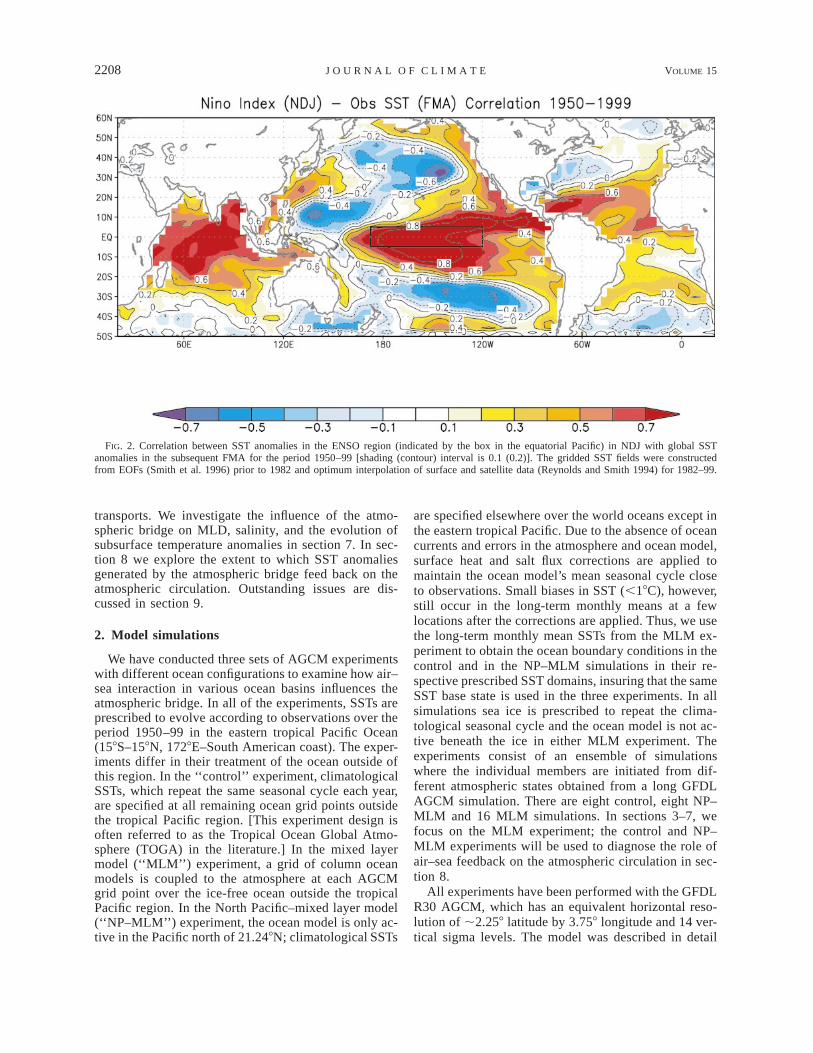
Beginning in the mid-1970s, researchers related ob-served SST anomalies in the tropical Pacific with anom-alies in other ocean basins, as summarized in Table 1.Using a wide range of techniques, the studies listed inTable 1 present convincing evidence that ENSO influ-ences the evolution of SST anomalies outside the equa-torial Pacific, especially in the North Pacific, tropicalAtlantic, and Indian Oceans. The global nature of theENSO SST signal, first noted by Pan and Oort (1983,1990), is illustrated here by Fig. 2, which shows the

correlations between SST anomalies averaged over58N–58S, 1728E–1208W (hereafter referred to as theENSO index) during November–December–January(NDJ) and SST anomalies over the global oceans duringthe following February–March–April (FMA). We chosethese periods since ENSO peaks near the end of thecalendar year (Rasmusson and Carpenter 1982), whilemost of the ENSO-related SST anomalies outside of thetropical Pacific peak 2–6 months later (Table 1). Thisone-to-two season lag occurs because the atmospheretakes ;2 weeks to respond to SST anomalies in thetropical Pacific and then the ocean integrates the forcingassociated with the atmospheric bridge over the nextseveral months.

While many of the relationships between SST anom-alies in the equatorial Pacific and those in other oceanbasins were recognized prior to 1990, the processes re-sponsible for the generation of the remote SST anom-alies and the feedback of the SST anomalies on theatmospheric circulation were not yet clear. A major goalof the Geophysical Fluid Dynamics Laboratory(GFDL)–University Consortium, since its establishmentin 1990, has been to improve our understanding of theimpact of both tropical and extratropical SSTs on globalclimate, primarily using atmospheric general circulationmodel (AGCM) experiments. Through the consortiumand other research efforts, our knowledge of the at-mospheric bridge and its role in climate variability hasadvanced considerably over the past decade.


TABLE 1. Observational studies, grouped by region, that have examined the relationship between SST anomalies in the equatorial Pacificwith those elsewhere over the global oceans. Also listed is the method of analyses, the period of record, months when the anomalies peakin the non-ENSO region, lag in months from when SST anomalies peak in the equatorial Pacific and the timescales of variability examined:interannual (I), decadal (D), if differentiated. The statistical methods are abbreviated: empirical orthogonal function (EOF), singular valuedecomposition (SVD), singular spectrum analyses (SSA), rotated principal component analyses (RPCA), canonical correlation analyses (CCA),linear inverse modeling (LIM).

Data

Study Record Method

Time

Months Lag Scale

North PacificWeare et al. (1976)Reynolds and Rassmusson (1983)Wright (1983)Niebauer (1984, 1988)Wallace and Jiang (1987)Hanawa et al. (1989)Deser and Blackmon (1995)Zhang and Wallace (1996)Nakamura et al. (1997)Zhang et al. (1998)

1949–731947–80

1950–791961–851950–921950–941951–921950–93

EOFsCompositesCorrelationsCorrelations in Bering SeaCorrelations with SOComposites, correlationsEOFsRegression, EOFs, Rotated EOFs, SVDPrefiltered EOFsMultichannel SSA

SON

Jul–NovJFMNov–Mar

2–3

DI/D

Tropical AtlanticCovey and Hastenrath (1978)Curtis and Hastenrath (1995)Enfield and Mayer (1997)Penland and Matrosova (1998)Uvo et al. (1998)Giannini et al. (2000)

1911–711948–921950–921950–931946–851861–1990

CompositesCompositesCorrelationsLIMSVDCCA

MAM

MarMAMJ

3–5

22–4

Global TropicsWolter (1987, 1989)Lanzante (1996)Toure and White (1995)Nicholson (1997)Klein et al. (1999)

1948–831870–19881979–911948–981952–92

Cluster analysis, RPCAComplex RPCA, correlationsEOFs, REOFsHarmonic analysis, compositesCorrelation

3–6

GlobalPan and Oort (1983, 1990)Hsiung and Newell (1983)Yasunari (1987)Kiladis and Diaz (1989)Nitta and Yamada (1989)Kawamura (1994)Zhang et al. (1997)Moron et al. (1998)*Enfield and Mestas-Nunez (1999)Mestas-Nunez and Enfield (1999)Garreaud and Battisti (1999)

1958–731949–791964–811877–19881950–871950–881900–931901–941856–19911856–19911958–93

CorrelationsEOFSPrefiltered compositesCompositesEOFs, difference mapsRotated EOFsRegressions, EOFsMultichannel SSAPrefiltered complex EOFsPrefiltered rotated EOFsRegressions

0–6

I

I/D

I/DI/DI/DDI/D

* Lists additional publications that have examined observed SST relationships.

This paper is intended to serve as a review of thestate of our understanding of the atmospheric bridge. Inthe context of our review, we will present results fromnew observational analyses and atmosphere–oceanmodel experiments, which will illustrate advances thathave been made in the past and outstanding issues thatremain. In particular, we will assess the influence of air–sea feedback on the original atmospheric response toENSO in the Pacific–North American (PNA) region,which has differed among previous modeling studies(cf. Alexander 1992b; Blade 1999; Lau and Nath 1996,2001), and examine emerging issues such as the rela-tionship between SST anomalies in the equatorial andNorth Pacific Ocean at low frequencies and the extentto which the bridge influences upper–ocean conditions

besides SSTs. While a global perspective of the bridgeis provided, our primary focus is on ENSO-relatedanomalies in the PNA region.

We briefly describe the atmosphere and ocean modelsand the experimental design in section 2. In section 3we examine the global precipitation and atmosphericcirculation changes resulting from the tropical SSTanomalies. ENSO-related SST anomalies on interannualand decadal timescales are investigated in section 4,while section 5 examines the atmospheric bridgethrough the relationship between sea level pressure(SLP) and SST. In section 6, we consider how changesin the atmosphere associated with ENSO can create SSTanomalies via surface energy fluxes, entrainment of sub-surface waters into the surface mixed layer, and Ekman


FIG. 2. Correlation between SST anomalies in the ENSO region (indicated by the box in the equatorial Pacific) in NDJ with global SSTanomalies in the subsequent FMA for the period 1950–99 [shading (contour) interval is 0.1 (0.2)]. The gridded SST fields were constructedfrom EOFs (Smith et al. 1996) prior to 1982 and optimum interpolation of surface and satellite data (Reynolds and Smith 1994) for 1982–99.

transports. We investigate the influence of the atmo-spheric bridge on MLD, salinity, and the evolution ofsubsurface temperature anomalies in section 7. In sec-tion 8 we explore the extent to which SST anomaliesgenerated by the atmospheric bridge feed back on theatmospheric circulation. Outstanding issues are dis-cussed in section 9.

2. Model simulations

We have conducted three sets of AGCM experimentswith different ocean configurations to examine how air–sea interaction in various ocean basins influences theatmospheric bridge. In all of the experiments, SSTs areprescribed to evolve according to observations over theperiod 1950–99 in the eastern tropical Pacific Ocean(158S–158N, 1728E–South American coast). The exper-iments differ in their treatment of the ocean outside ofthis region. In the ‘‘control’’ experiment, climatologicalSSTs, which repeat the same seasonal cycle each year,are specified at all remaining ocean grid points outsidethe tropical Pacific region. [This experiment design isoften referred to as the Tropical Ocean Global Atmo-sphere (TOGA) in the literature.] In the mixed layermodel (‘‘MLM’’) experiment, a grid of column oceanmodels is coupled to the atmosphere at each AGCMgrid point over the ice-free ocean outside the tropicalPacific region. In the North Pacific–mixed layer model(‘‘NP–MLM’’) experiment, the ocean model is only ac-tive in the Pacific north of 21.248N; climatological SSTs

are specified elsewhere over the world oceans except inthe eastern tropical Pacific. Due to the absence of oceancurrents and errors in the atmosphere and ocean model,surface heat and salt flux corrections are applied tomaintain the ocean model’s mean seasonal cycle closeto observations. Small biases in SST (,18C), however,still occur in the long-term monthly means at a fewlocations after the corrections are applied. Thus, we usethe long-term monthly mean SSTs from the MLM ex-periment to obtain the ocean boundary conditions in thecontrol and in the NP–MLM simulations in their re-spective prescribed SST domains, insuring that the sameSST base state is used in the three experiments. In allsimulations sea ice is prescribed to repeat the clima-tological seasonal cycle and the ocean model is not ac-tive beneath the ice in either MLM experiment. Theexperiments consist of an ensemble of simulationswhere the individual members are initiated from dif-ferent atmospheric states obtained from a long GFDLAGCM simulation. There are eight control, eight NP–MLM and 16 MLM simulations. In sections 3–7, wefocus on the MLM experiment; the control and NP–MLM experiments will be used to diagnose the role ofair–sea feedback on the atmospheric circulation in sec-tion 8.

All experiments have been performed with the GFDLR30 AGCM, which has an equivalent horizontal reso-lution of ;2.258 latitude by 3.758 longitude and 14 ver-tical sigma levels. The model was described in detail


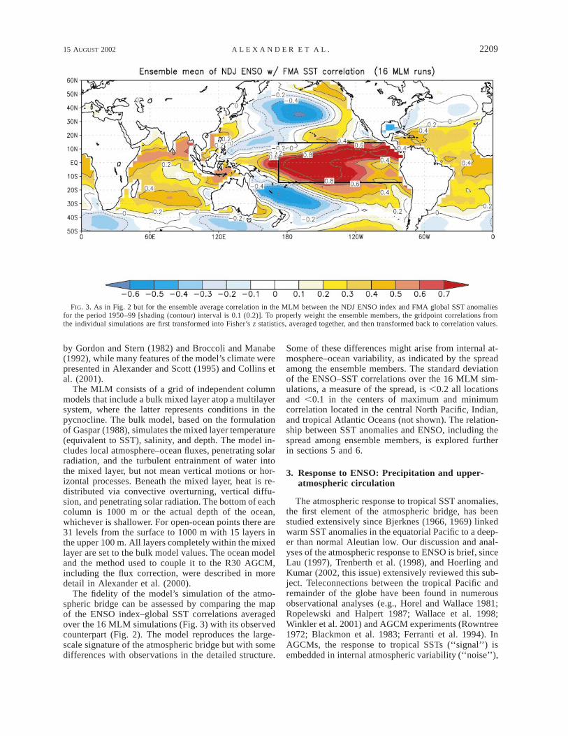
FIG. 3. As in Fig. 2 but for the ensemble average correlation in the MLM between the NDJ ENSO index and FMA global SST anomaliesfor the period 1950–99 [shading (contour) interval is 0.1 (0.2)]. To properly weight the ensemble members, the gridpoint correlations fromthe individual simulations are first transformed into Fisher’s z statistics, averaged together, and then transformed back to correlation values.

by Gordon and Stern (1982) and Broccoli and Manabe(1992), while many features of the model’s climate werepresented in Alexander and Scott (1995) and Collins etal. (2001).

The MLM consists of a grid of independent columnmodels that include a bulk mixed layer atop a multilayersystem, where the latter represents conditions in thepycnocline. The bulk model, based on the formulationof Gaspar (1988), simulates the mixed layer temperature(equivalent to SST), salinity, and depth. The model in-cludes local atmosphere–ocean fluxes, penetrating solarradiation, and the turbulent entrainment of water intothe mixed layer, but not mean vertical motions or hor-izontal processes. Beneath the mixed layer, heat is re-distributed via convective overturning, vertical diffu-sion, and penetrating solar radiation. The bottom of eachcolumn is 1000 m or the actual depth of the ocean,whichever is shallower. For open-ocean points there are31 levels from the surface to 1000 m with 15 layers inthe upper 100 m. All layers completely within the mixedlayer are set to the bulk model values. The ocean modeland the method used to couple it to the R30 AGCM,including the flux correction, were described in moredetail in Alexander et al. (2000).

The fidelity of the model’s simulation of the atmo-spheric bridge can be assessed by comparing the mapof the ENSO index–global SST correlations averagedover the 16 MLM simulations (Fig. 3) with its observedcounterpart (Fig. 2). The model reproduces the large-scale signature of the atmospheric bridge but with somedifferences with observations in the detailed structure.

Some of these differences might arise from internal at-mosphere–ocean variability, as indicated by the spreadamong the ensemble members. The standard deviationof the ENSO–SST correlations over the 16 MLM sim-ulations, a measure of the spread, is ,0.2 all locationsand ,0.1 in the centers of maximum and minimumcorrelation located in the central North Pacific, Indian,and tropical Atlantic Oceans (not shown). The relation-ship between SST anomalies and ENSO, including thespread among ensemble members, is explored furtherin sections 5 and 6.

3. Response to ENSO: Precipitation and upper-atmospheric circulation

The atmospheric response to tropical SST anomalies,the first element of the atmospheric bridge, has beenstudied extensively since Bjerknes (1966, 1969) linkedwarm SST anomalies in the equatorial Pacific to a deep-er than normal Aleutian low. Our discussion and anal-yses of the atmospheric response to ENSO is brief, sinceLau (1997), Trenberth et al. (1998), and Hoerling andKumar (2002, this issue) extensively reviewed this sub-ject. Teleconnections between the tropical Pacific andremainder of the globe have been found in numerousobservational analyses (e.g., Horel and Wallace 1981;Ropelewski and Halpert 1987; Wallace et al. 1998;Winkler et al. 2001) and AGCM experiments (Rowntree1972; Blackmon et al. 1983; Ferranti et al. 1994). InAGCMs, the response to tropical SSTs (‘‘signal’’) isembedded in internal atmospheric variability (‘‘noise’’),


FIG. 4. Regression values of precipitation (shaded; interval is 0.5 mm day21 8C21) and 200-mb streamfunction(contour; interval is 1 3 106 m2 day21 8C21) regressed on DJF ENSO index for DJF (1951–99) for (a) observationand (b) MLM. Changes in the nondivergent component of the upper-tropospheric circulation accompanying ENSOmay be inferred from the contour lines: positive (negative) extremes are associated with anomalous clockwise (coun-terclockwise) flows.

requiring either long simulations or a large ensemble ofsimulations to obtain statistically significant results (Ku-mar and Hoerling 1998; Sardeshmukh et al. 2000). Thedynamical link between the Tropics and extratropics in-volves the excitation of Rossby waves by both tropicalconvection (Hoskins and Karoly 1981) and the asso-ciated divergent outflow in regions of strong vorticitygradients (Sardeshmukh and Hoskins 1988). The per-turbations that propagate to the extratropics are furtherinfluenced by interactions with asymmetries in the zonalmean flow (Simmons et al. 1983; Ting and Sardeshmukh1993) and with midlatitude storm tracks (Kok and Op-steegh 1985; Held et al. 1989).

The atmospheric anomalies associated with equatorialPacific SST anomalies are shown in Fig. 4 by regressingprecipitation (color shading) and 200-mb streamfunc-

tion (contours) on the ENSO index during December–January–February (DJF). The observed fields in Fig. 4are based on winds from the National Centers for En-vironmental Prediction–National Center for Atmospher-ic Research (NCEP–NCAR) reanalysis project (Kalnayet al. 1996; Kistler et al. 2001) and the precipitationfrom the Climate Prediction Center (CPC) MergedAnalysis of Precipitation (CMAP) dataset (Xie and Ar-kin 1997), while the corresponding simulated fields arefrom the 16-member ensemble means of the MLM ex-periment.

During El Nino (warm ENSO) events, both the ob-served and model precipitation patterns are character-ized by enhanced rainfall over the central equatorialPacific and below-normal rainfall over Indonesia/west-ern tropical Pacific and northern Brazil. The simulated


precipitation anomalies between 908E and 1808 areweaker and of smaller extent than in nature. A pair ofanticyclones straddles the positive precipitation centerover the central equatorial Pacific, similar to the at-mospheric response to diabatic heating on the equatorin shallow-water models (Matsuno 1966; Gill 1980).The anomalous westward flow along the equator eastof the date line indicates eastward displacement of theWalker circulation during warm events. The extratrop-ical flow is characterized by enhanced westerlies from208 to 408 latitude in both the North and South Pacific,and by wavelike features with centers in the northeasternPacific, Canada, eastern United States, and southernChina. The MLM reproduces most of these featuresquite accurately, although the streamfunction anomaliesover the tropical Pacific are displaced west of their ob-served locations. The precipitation and circulationanomalies from the GFDL R15 (;4.458 latitude 3 7.58longitude) AGCM, the model used in many previousconsortium studies, were substantially weaker than theR30 estimates.

4. ENSO-related SST anomalies

Along with enhanced comprehension of atmosphericENSO teleconnections, another key development in theatmospheric bridge hypothesis was identifying relation-ships between SST anomalies in various parts of theglobal ocean and those in the equatorial Pacific. Pre-vious research focused on SST anomalies in the NorthPacific, tropical North Atlantic, and Indian Oceans,where the ENSO signal is strong (Table 1, Fig. 2).

a. North Pacific

The relationship between SST anomalies in the trop-ical and North Pacific was first revealed by Weare et al.(1976) through EOF analyses of SST anomalies in allcalendar months. This study, as well as more recent EOFanalyses (e.g., Deser and Blackmon 1995; Zhang andWallace 1996), found that the dominant pattern of Pa-cific SST variability has anomalies of one sign in theequatorial Pacific and along the coast of North Americaand anomalies of the opposite sign extending from;1408W to the coast of Asia between about 258 and508N. The corresponding principal component [(PC),which shows the amplitude and polarity of the patternover time] indicates that during El Nino events anom-alously warm (cold) water occurs in the eastern (central)North Pacific and vice versa during La Nina events.Other observational analyses confirmed the EOF resultsand established that ENSO-related SST anomalies occurin the Bering Sea (Niebauer 1984, 1988) and SouthChina Sea (Hanawa et al. 1989) in winter and in theNorth Pacific during summer/fall (Reynolds and Ras-musson 1983; Wallace and Jiang 1987). The former alsoappear in Figs. 2 and 3, while the evolution of the SST

anomalies over the seasonal cycle is discussed furtherin section 5.

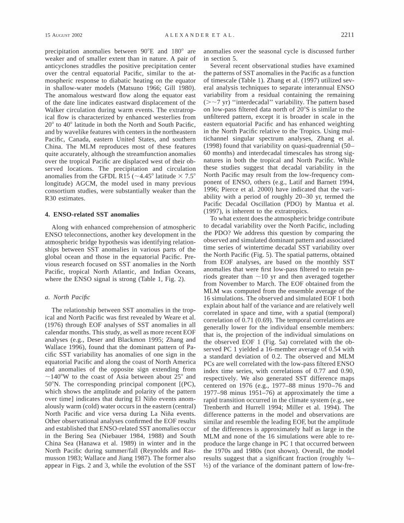
Several recent observational studies have examinedthe patterns of SST anomalies in the Pacific as a functionof timescale (Table 1). Zhang et al. (1997) utilized sev-eral analysis techniques to separate interannual ENSOvariability from a residual containing the remaining(.;7 yr) ‘‘interdecadal’’ variability. The pattern basedon low-pass filtered data north of 208S is similar to theunfiltered pattern, except it is broader in scale in theeastern equatorial Pacific and has enhanced weightingin the North Pacific relative to the Tropics. Using mul-tichannel singular spectrum analyses, Zhang et al.(1998) found that variability on quasi-quadrennial (50–60 months) and interdecadal timescales has strong sig-natures in both the tropical and North Pacific. Whilethese studies suggest that decadal variability in theNorth Pacific may result from the low-frequency com-ponent of ENSO, others (e.g., Latif and Barnett 1994,1996; Pierce et al. 2000) have indicated that the vari-ability with a period of roughly 20–30 yr, termed thePacific Decadal Oscillation (PDO) by Mantua et al.(1997), is inherent to the extratropics.

To what extent does the atmospheric bridge contributeto decadal variability over the North Pacific, includingthe PDO? We address this question by comparing theobserved and simulated dominant pattern and associatedtime series of wintertime decadal SST variability overthe North Pacific (Fig. 5). The spatial patterns, obtainedfrom EOF analyses, are based on the monthly SSTanomalies that were first low-pass filtered to retain pe-riods greater than ;10 yr and then averaged togetherfrom November to March. The EOF obtained from theMLM was computed from the ensemble average of the16 simulations. The observed and simulated EOF 1 bothexplain about half of the variance and are relatively wellcorrelated in space and time, with a spatial (temporal)correlation of 0.71 (0.69). The temporal correlations aregenerally lower for the individual ensemble members:that is, the projection of the individual simulations onthe observed EOF 1 (Fig. 5a) correlated with the ob-served PC 1 yielded a 16-member average of 0.54 witha standard deviation of 0.2. The observed and MLMPCs are well correlated with the low-pass filtered ENSOindex time series, with correlations of 0.77 and 0.90,respectively. We also generated SST difference mapscentered on 1976 (e.g., 1977–88 minus 1970–76 and1977–98 minus 1951–76) at approximately the time arapid transition occurred in the climate system (e.g., seeTrenberth and Hurrell 1994; Miller et al. 1994). Thedifference patterns in the model and observations aresimilar and resemble the leading EOF, but the amplitudeof the differences is approximately half as large in theMLM and none of the 16 simulations were able to re-produce the large change in PC 1 that occurred betweenthe 1970s and 1980s (not shown). Overall, the modelresults suggest that a significant fraction (roughly ¼–½) of the variance of the dominant pattern of low-fre-


FIG. 5. EOF 1 of the low-pass filtered (.;10 yr) SST during Nov–Mar from (a) observations and (b) the MLM.(c) The first PC (time series associated with EOF 1) of the filtered SST from observations (green line), the MLM(blue line), and the ENSO index (black line). The correlations (r) between the three time series are given above (c).

quency SST variability in the North Pacific is associatedwith the atmospheric bridge.

The patterns in Fig. 5 are very similar to the dominantpattern based on unfiltered data (not shown), whichMantua et al. (1997) used to define the PDO. Processesother than the atmospheric bridge, including stochasticatmospheric forcing of the ocean and perhaps midlati-

tude air–sea interaction, also influence the leading pat-tern of North Pacific SST variability. Thus, the PDOlikely includes both tropical and extratropical sourcesof decadal variability. Other parts of the North Pacificmay be more independent from tropical influence: Deserand Blackmon (1995) and Nakamura et al. (1997) foundthat decadal variability in the North Pacific concentrated


along the subarctic front (;428N, 1458E–1708W) wasuncorrelated with tropical SST variability.

b. Tropical Atlantic

The link between SST anomalies in the equatorialPacific and those in other tropical ocean basins was firstexamined shortly after the Weare et al. (1976) study.Using SST anomalies off the Peruvian coast as a mea-sure of ENSO, Covey and Hastenrath (1978) constructedcomposites of SST, SLP, and winds in the tropical At-lantic. They found a broad region of warm SSTs to thenorth of the equator in boreal spring following El Ninoevents and roughly the opposite after La Nina events.Many subsequent observational analyses (Curtis andHastenrath 1995; Lanzante 1996; Enfield and Mayer1997; Klein et al. 1999; our Fig. 2) confirmed that pos-itive SST anomalies occur in the north tropical Atlanticand Caribbean during boreal spring, approximately 3–6 months following the peak in tropical Pacific SSTanomalies. Some studies (e.g., Enfield and Mayer 1997;Nicholson 1997) have found links between ENSO andSSTs in the equatorial and South Atlantic, but theserelationships are weak and may not be significant.

c. Indian Ocean

Like the tropical Atlantic, the Indian Ocean warmsduring El Nino, with SST anomalies in that basin lag-ging those in the central Pacific by about 3–6 months(Lanzante 1996; Klein et al. 1999). Warming in theIndian Ocean begins earlier than in the Atlantic, startingduring boreal summer/fall of the El Nino year. Overperiods of 2.5–6 yr, Indian Ocean SSTs have significantvariability that is coherent with Southern Oscillationfluctuations (Cadet 1985; Nicholson 1997). Addition-ally, the two leading patterns of SST variability in theIndian Ocean are associated with ENSO (Tourre andWhite 1995; Murtugudde and Busalachi 1999). For ex-ample, during the closing stage of a very strong El Ninoevent in 1998, SST anomalies exceeded 18C over mostof the Indian Ocean north of 208S (Yu and Rienecker1999). Prior to this basinwide warming, a dipole SSTanomaly pattern developed along the equator during theprevious fall, with positive (negative) anomalies in thewestern (eastern) Indian Ocean. Yu and Rienecker pro-posed that the dipole pattern is directly related to chang-es in the Walker circulation during ENSO, while Sajiet al. (1999) and Webster et al. (1999) suggested thatthe dipole mode is independent of ENSO and is causedby local air–sea interaction.

5. SLP–SST relationships: The bridge revealed

Until the mid-1980s, studies of ENSO-related at-mospheric and oceanic anomalies that formed outsideof the tropical Pacific progressed on separate tracks. Thetwo were linked by investigators who noted the close

association between SST anomalies and the overlyingSLP or surface wind anomalies during El Nino events.

The relationship between the Southern Oscillation in-dex (SOI, normalized Tahiti–Darwin SLP) and globalsea level pressure variations has been known since earlyin the twentieth century (e.g., Lockyer and Lockyer1902; Walker 1909, 1924; Walker and Bliss 1932). Na-mias (1976), Trenberth and Paolino (1981), and vanLoon and Madden (1981) confirmed many of the find-ings from the early inquiries, noting statistically sig-nificant relationships between various ENSO indicesand SLP in the North Pacific during winter and spring.Simpson (1983) suggested that atmospheric teleconnec-tions during the 1982/83 El Nino event drove changesin the California current system. Emery and Hamilton(1985) synthesized these studies with those concerninglarge-scale ENSO–SST relationships (e.g., Weare et al.1976; Pan and Oort 1983) and proposed that ‘‘the trop-ical Pacific Ocean may interact with the North Pacificvia an atmospheric link.’’ They concluded that a stron-ger Aleutian low during El Nino events could accountfor anomalously warm ocean temperatures in the north-east Pacific. As a corollary, when the North Pacific SLPanomalies differ from the canonical ENSO signal, whichis not unusual (Emery and Hamilton 1985; Hanawa etal. 1989), then the corresponding SST patterns will alsobe different.

Two different modeling strategies were used to cor-roborate the atmospheric link between SST anomaliesin the equatorial and North Pacific Ocean. Luksch et al.(1990) and Luksch and von Storch (1992) used an oceanGCM forced with observed surface winds and a simpleatmospheric boundary layer model to estimate surfaceair temperature. Alexander (1990) used output from anatmospheric GCM, with and without warm SSTs spec-ified as boundary conditions in the tropical Pacific, todrive a grid of one-dimensional mixed layer models inthe North Pacific Ocean. In a follow-up experiment,Alexander (1992a) coupled the North Pacific Oceanmodel to the same AGCM. Both Luksch et al. and Al-exander found that changes in the near-surface circu-lation associated with El Nino induced an SST patternin the North Pacific that resembled observations, withcold water in the central North Pacific and warm waterin the Gulf of Alaska. While these studies clearly val-idated the atmospheric link between the tropical andNorth Pacific during ENSO, Lau and Nath (1994) werethe first to call this process the atmospheric bridge.

Following Rasmusson and Carpenter (1982) and Har-rison and Larkin (1998), we use composite analysis toshow the evolution of SLP and SST over the life cycleof ENSO events. Composites are constructed based onnine El Nino (warm) events: 1957, 1965, 1969, 1972,1976, 1982, 1987, 1991, and 1997; and nine La Nina(cold) events: 1950, 1954, 1955, 1964, 1970, 1973,1975, 1988, and 1998. The first eight El Nino and LaNina events were identified by Trenberth (1997), towhich we added the 1997 El Nino and 1998 La Nina


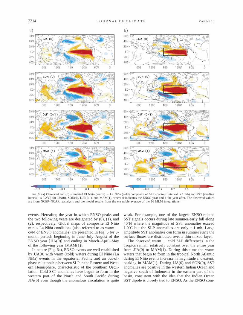
FIG. 6. (a) Observed and (b) simulated El Nino (warm) 2 La Nina (cold) composite of SLP (contour interval is 1 mb) and SST (shadinginterval is 0.28C) for JJA(0), SON(0), DJF(0/1), and MAM(1), where 0 indicates the ENSO year and 1 the year after. The observed valuesare from NCEP–NCAR reanalysis and the model results from the ensemble average of the 16 MLM integrations.

events. Hereafter, the year in which ENSO peaks andthe two following years are designated by (0), (1), and(2), respectively. Global maps of composite El Ninominus La Nina conditions (also referred to as warm 2cold or ENSO anomalies) are presented in Fig. 6 for 3-month periods beginning in June–July–August of theENSO year [JJA(0)] and ending in March–April–Mayof the following year [MAM(1)].

In nature (Fig. 6a), ENSO events are well establishedby JJA(0) with warm (cold) waters during El Nino (LaNina) events in the equatorial Pacific and an out-of-phase relationship between SLP in the Eastern and West-ern Hemisphere, characteristic of the Southern Oscil-lation. Cold SST anomalies have begun to form in thewestern part of the North and South Pacific duringJJA(0) even though the anomalous circulation is quite

weak. For example, one of the largest ENSO-relatedSST signals occurs during late summer/early fall along408N where the magnitude of SST anomalies exceed1.08C but the SLP anomalies are only ;1 mb. Largeamplitude SST anomalies can form in summer since thesurface fluxes are distributed over a thin mixed layer.

The observed warm 2 cold SLP differences in theTropics remain relatively constant over the entire yearfrom JJA(0) to MAM(1). During this time the warmwaters that begin to form in the tropical North Atlanticduring El Nino events increase in magnitude and extent,peaking in MAM(1). During JJA(0) and SON(0), SSTanomalies are positive in the western Indian Ocean andnegative south of Indonesia in the eastern part of thebasin, consistent with the idea that the Indian OceanSST dipole is closely tied to ENSO. As the ENSO com-


posite progresses, warm water spreads throughout theIndian Ocean and South China Sea.

In the northern extratropics, the SLP anomalies arestrongest during December(0)–February(1) [DJF(0/1)]when the Aleutian low is 9 mb deeper during El Ninothan in La Nina events (Fig. 6a). As a result, surfacewesterlies are enhanced over the central North Pacific.During El Nino, anomalous northwesterly winds advectcold air over the central North Pacific, while southerlywinds advect warm moist air along the west coast ofNorth America. The negative (positive) temperature de-partures in the central (eastern) North Pacific are con-sistent with this surface forcing.

The corresponding evolution of SLP and SST anom-alies during ENSO from the ensemble average of the16 MLM simulations is shown in Fig. 6b. The modelreproduces many of the features found in the observedcomposite, especially in DJF(0/1)–MAM(1), whichhelps to confirm the essence of the atmospheric bridgehypothesis: that is, local atmospheric forcing is the pri-mary factor in generating SST anomalies outside thetropical Pacific during ENSO. However, several dis-crepancies between the model and observations can benoted as well. For example, the simulated negative SLPanomalies over the North Pacific are of greater mag-nitude and extent than in observations in JJA(0),SON(0), and MAM(1), while the reverse is true inDJF(0/1). While some of the model–data differencescould be due to internal atmospheric variability, as sug-gested by the spread among ensemble members (see Fig.8), many of the differences are likely caused by modelerror and the absence of ocean dynamics.

6. Processes that generate SST anomalies

The atmosphere influences SST directly through sur-face heat fluxes and indirectly via momentum and fresh-water fluxes, which subsequently affect ocean currentsand turbulent mixing. Here we examine air–sea inter-actions in the North Pacific, tropical Atlantic, and IndianOceans, where the atmospheric bridge has been shownto be strong.

a. North Pacific

The very strong but unanticipated 1982/83 El Ninoevent forced researchers to reconsider not only the fun-damental dynamics of ENSO but also how ocean anom-alies develop in the extratropical Pacific. Prior to the1982/83 event, research focused on coastal Kelvinwaves as the mechanism for linking tropical and extra-tropical SST anomalies during ENSO. These waves,however, are confined to a narrow region near the shore;for example, the internal deformation radius (e-foldingscale) of coastal Kelvin waves is less than 50 (20) kmat 208N (458N). While Rienecker and Mooers (1986)and Johnson and O’Brien (1990) confirmed the impor-tance of coastally trapped waves, they, along with Simp-

son (1983) and Wagner (1984), showed that changes inthe atmospheric circulation played a major role in al-tering oceanic conditions along the west coast of NorthAmerica during the 1982/83 event.

In a review of El Nino, Mysak (1986) hypothesizedseveral ways in which changes in the near-surface at-mospheric circulation over the North Pacific could in-fluence SSTs: coastal upwelling, Ekman pumping, andocean advection—presumably through Ekman trans-port. Mysak and the studies mentioned above, however,did not consider surface heat fluxes. The relationshipbetween ENSO and surface fluxes was investigated byZhao and McBean (1986) and Cayan (1990), who cor-related the SOI with air–sea heat fluxes over the NorthPacific and the globe, respectively. Zhao and McBeanfound only a weak relationship between the SOI andsurface fluxes, while Cayan found significant correla-tions with fluxes in the central North Pacific. The dis-crepancy between these two studies could result fromdifferences in the period of record, the number and qual-ity of the observations used in the analyses, and thecoefficients used in the bulk formulas to compute thefluxes. Subsequent studies of surface fluxes (e.g., Iwa-saka and Wallace 1995) have tended to confirm Cayan’sanalyses.

Frankignoul (1985), Qiu (2000), and Scott (2002,manuscript submitted to J. Climate) discussed factorsthat influence the evolution of extratropical SST anom-alies. Here we consider the three dominant factors oninterannual timescales: the net surface heat flux (Qnet),entrainment heat flux (Qwe), and Ekman transport (Qek).Alexander (1990, 1992a) showed that Qnet was the dom-inant process in generating SST anomalies in the NorthPacific during ENSO, while Lau and Nath (1994, 1996,2001) found that these SST anomalies could be fairlywell simulated by a 50-m slab model forced only withsurface heat fluxes. Neither study considered Qek. Theanomalous Ekman heat transport, which depends pri-marily on the anomalous surface wind stress multipliedby the mean SST gradient, is computed here as a di-agnostic, that is, it does not influence SST in the MLM.

The MLM warm 2 cold composites of Qnet, Qwe, andQek during DJF (0/1) are shown in Fig. 7. Clearly, Qnet

is the dominant factor creating SST anomalies duringboreal winter, which explains why studies that use fixed-depth ocean models can simulate SST anomalies as-sociated with ENSO reasonably well. Consistent withthe low-level atmospheric circulation (Fig. 6b), the sur-face fluxes cool the central North Pacific and warm theGulf of Alaska and South China Sea during El Nino.In these regions | Qnet | . 40 W m22, which leads toSST tendencies of ;0.258C month21 for a typical win-tertime MLD of 100 m; thus slab models where theMLD is set to 50 m overestimate the amplitude of SSTanomalies in winter.

Consistent with Alexander (1990, 1992a), the maxi-mum Qwe anomalies are roughly ¼–⅓ as large as thoseof Qnet (Fig. 7) but have a different pattern. During


FIG. 7. The composite El Nino 2 La Nina (a) net heat flux to the ocean (Qnet), (b) entrainment heat flux (Qwe), (c)Ekman heat transport composites (Qek) during DJF(0/1) from the MLM. The shading (contour) interval is 5 (10) Wm22. The box in (c) delineates the central North Pacific region.

winter, Qwe slightly enhances the cold anomaly in thecentral North Pacific, but primarily damps the SSTanomalies over the remainder of the basin. In the oceanmodel, Qwe 5 (we/MLD)(Tbelow 2 SST), where we is theentrainment rate and Tbelow is the temperature just belowthe mixed layer. Given that the time mean MLD and we

are always positive, if the we and Tbelow departures fromthe time mean (9) are relatively small, then øQ9we

2 eSST9/ , which indicates that the anomalousw MLDheat flux at the base of the mixed layer tends to dampSST anomalies. While this is often the case (Frankignouland Reynolds 1983), entrainment can also generate SSTanomalies, depending on the season and vertical tem-perature structure (see section 7c).

The diagnosed Ekman heat transport is generally inphase with Qnet but approximately ⅓–½ as large. En-hanced westerlies in the central North Pacific during El

Nino, which increase the upward surface heat flux, alsocool the water through southward Ekman drift. The di-agnosed MLM Qek anomalies are similar to observationsbut the cooling over the central North Pacific is some-what stronger in nature (not shown).

The net surface heat flux is composed of shortwave(Qsw) and longwave (Qlw) radiation and sensible (Qsh)and latent (Qlh) heat flux. In mid- and high latitudes,sensible and latent heat fluxes dominate the generationof SST anomalies in fall and winter during ENSO (Al-exander 1992a; Lau and Nath 2001). In general, Qlh

anomalies strongly influence SST over the entire globe,while the magnitude of the Qsh (Qsw) anomalies increases(decreases) when going from the Tropics toward thePoles.

The evolution of ENSO-induced SST anomalies andassociated forcing terms over a region in the central


FIG. 8. Composite El Nino 2 La Nina time series of SST (8C) andfluxes into the mixed layer (W m22) over the ENSO cycle for a regionin the central North Pacific (288–428N, 1808–1608W). (a) SST and(b) (Qlh 1 Qsh) heat flux from NCEP reanalysis (green), the ensemblemean MLM (solid black), and the 16 individual MLM simulations(black crosses); (c) Qnet (black), Qwe (green), Qek (blue) from the MLM;and (d) the four components of Qnet from the MLM: Qsw (red), Qlw

(blue), Qsh (black), and Qlh (green). All curves have been smoothedusing a three-month running average.

North Pacific (288–428N, 1808–1608W, box in Fig. 7c)is shown in Fig. 8. During fall and winter, Qlh and Qsh,and to a lesser extent, Qsw, cool the mixed layer. Whilethe model accurately simulates the magnitude of the SSTanomalies in Feb(1)–May(1), it underestimates the cool-ing from Sep(0)–Jan(1), even when the spread amongthe 16 ensemble members is taken into account (Fig.8a). The limited magnitude of the simulated SST anom-alies in fall is somewhat surprising given that the coolingdue to Qsh 1 Qlh is greater in the MLM than in theNCEP–NCAR reanalysis beginning in Aug(0) (Fig. 8b).Several factors may contribute to the underestimate ofthe SST anomaly in the central North Pacific: (i) errorsin simulated radiative fluxes, especially Qsw, (Scott andAlexander 1999); (ii) an overestimation of MLD in theMLM resulting in a reduced SST anomaly, although the

simulated MLD is close to observed during fall andwinter in this region; (iii) amplifying feedbacks betweenmodel errors; and (iv) processes absent from the MLM,such as Ekman transport. While the diagnosed Qek doescool the central Pacific region in late fall/early winter(Fig. 8c), other factors must contribute to the model–data differences in Sep(0)–Nov(0).

In the central North Pacific region, cooling by Qwe

and Qlh (Figs. 8c,d) is slightly larger than the warmingdue to Qsw during the summer of Yr(0). Even thoughthe flux anomalies are of limited magnitude they cansignificantly affect SSTs in summer since the mixedlayer is shallow (,20 m).

b. Atlantic Ocean

During the last half of the 1990s several studies in-vestigated the processes responsible for the warming(cooling) of the tropical North Atlantic in boreal springfollowing the peak of El Nino (La Nina) events. Ob-servational analyses (Hastenrath et al. 1987; Curtis andHastenrath 1995; Enfield and Mayer 1997; Klein et al.1999) showed that weakening trade winds over muchof the Atlantic between approximately 58 and 208N re-duced the upward latent heat flux during JFM(1). TheAGCM simulations of Saravanan and Chang (2000) re-produced this finding but indicated that higher humidityassociated with warmer surface air temperature alsocontributes to the reduced evaporation. A reduction incloudiness (Klein et al. 1999; Lau and Nath 2001), as-sociated with both the descending branch of the anom-alous Walker circulation and with the atmospheric tele-connections that pass through the PNA sector, resultsin the warming of the subtropical North Atlantic inspring via enhanced Qsw. ENSO may also influence SSTsin the tropical Atlantic via changes in Ekman pumping(Curtis and Hastenrath 1995) and ocean dynamics (Latifand Barnett 1995). However, Klein et al. (1999) wereable to reproduce much of the observed warming as-sociated with ENSO using only surface flux anomaliesand a linear damping term. The results from the MLMsimulations (Fig. 7) indicate that Qnet has a much largereffect on SST anomalies than Qwe and Qek in the sub-tropical North Atlantic in DJF(0/1). In the Gulf of Mex-ico and eastern seaboard of the United States, large Qnet

anomalies (Fig. 7) are primarily due to anomalies in Qsw

and Qlh (not shown).

c. Indian Ocean

Surface heat fluxes also force SST anomalies in theNorth Indian Ocean and South China Sea during ENSOas illustrated by Fig. 7. Cadet (1985) and Klein et al.(1999) emphasized the role of shortwave fluxes in thisregion, while the observational analyses of Yu and Ri-enecker (1999) and modeling studies by Behera et al.(2000) and Venzke et al. (2000) indicated that latentheat fluxes are the dominant term driving SST anom-


FIG. 9. MLD (m) in JFM regressed on the DJF ENSO SST derivedfrom (a) subsurface temperature measurements from White (1995)and (b) the MLM. Both are shown for 1956–96, the period whenobservations are available.

alies. Ocean dynamics also appear to influence ENSO-related SST in parts of the Indian Ocean: easterly windanomalies enhance cooling in the eastern half of thebasin during SON(0) via Ekman pumping (Yu and Ri-enecker 1999), while Rossby waves generated by anom-alous winds in the southeastern Indian Ocean may con-tribute to the basinwide warming in the following winter(Chambers et al. 1999). The absence of ocean dynamicsmay partially explain why the MLM underestimates thepositive SST anomalies between 08 and 158S in the In-dian Ocean (cf. Figs. 6a and 6b).

7. Other ENSO-induced ocean changes

Most previous studies of the atmospheric bridge fo-cused on the development of SST anomalies, yet at-mospheric changes associated with ENSO also influencesalinity, mixed layer depth, and the subsurface temper-ature structure.

a. MLD

Regressions between the DJF ENSO index and MLDanomalies in JFM over the North Pacific are shown forobservations and the MLM in Fig. 9. The observedMLD provided by the Joint Environmental Data Anal-ysis Center (JEDAC; White 1995) is defined as the depthat which the temperature is 1.08C cooler than at thesurface and is based on bathythermograph measure-ments for the years 1956–96, while the MLD in theMLM is computed explicitly from the turbulent kineticenergy equation. The mean MLD is well simulated inthe North Pacific but is somewhat underestimated in theNorth Atlantic during winter (Alexander et al. 2000).

The observed and simulated patterns of ENSO-relatedMLD anomalies are similar, although the anomaly max-ima are shifted ;158 westward in the MLM, consistentwith the displacement of the model’s atmospheric re-sponse to tropical SST anomalies (Fig. 3). In both ob-servations and the MLM, the mixed layer is deeper inthe center of the basin and shallower in the northeastPacific and to the south and east of Japan. Hanawa etal. (1988) also noted shoaling of the mixed layer southof Japan during El Nino events. Over the North Pacificthe pattern in Fig. 9 resembles decadal changes in MLDduring winter (Polovina et al. 1995; Deser et al. 1996;Miller and Schneider 2000) as well as the ENSO SSTanomaly pattern (Figs. 2, 6, and 10) but with oppositepolarity. The magnitude of the simulated and observedanomalies is comparable over most of the domain, al-though the ENSO-related shoaling of the mixed layerwest of Canada is weaker in the MLM. While manyfactors are likely to contribute to the model–data dif-ferences in the MLD, a particularly important factor isthat salinity is included in the ocean model but not inthe observed MLD estimates. Salinity influences thedensity profile and hence the base of the mixed layer,especially north of ;458N.

b. Salinity

ENSO can influence salinity via precipitation minusevaporation (P 2 E), river runoff, and oceanic pro-cesses. Changes in P 2 E in the MLM result in largesalinity anomalies in the Tropics, where El Nino 2 LaNina salinity differences exceed 0.8 parts per thousand(ppt) in the Indonesian region from Jul(0)–Apr(1) and0.3 ppt in the Caribbean Sea from Oct(0)–Dec(0) (notshown). Schmittner et al. (2000) also found a decreasein P 2 E to the north of South America during El Ninoevents in the NCEP–NCAR and European Centre forMedium-Range Weather Forecasts (ECMWF) reanaly-sis datasets. Schmittner et al. (2000), Latif et al. (2000),and Latif (2000) presented evidence that P 2 E changesassociated with equatorial Pacific SST anomalies impactthe thermohaline circulation when the salinity anomaliesin the Caribbean are advected to the sinking regions inthe far North Atlantic. Lukas and Lindstrom (1991)found that salinity in the western equatorial Pacificstrongly influences the density profile and thus theamount of cooling due to entrainment during westerlywind bursts. They hypothesized that regulation of SSTin the warm pool region by salinity-dependent entrain-ment could play an important role in the ENSO cycle.

c. Reemergence of SST anomalies

The seasonal cycle of MLD has the potential to in-fluence upper-ocean temperatures from one winter tothe next. Namias and Born (1970, 1974) first noted thatmidlatitude SST anomalies tended to recur from onewinter to the next without persisting through the inter-


FIG. 10. El Nino 2 La Nina composite of SST over the North Pacific in Feb(1)–Mar(1), Aug(1)–Sep(1), and Dec(1)–Jan(2) from (left)observations and (right) the ensemble mean MLM. (bottom) The observed El Nino 2 La Nina composite SST in the tropical Pacific inDec(1)–Jan(2). The shading (contour) interval is 0.1 (0.2) 8C.

vening summer. They speculated that temperature anom-alies that form at the surface and spread throughout thedeep winter mixed layer remain beneath the mixed layerwhen it shoals in spring. The thermal anomalies areincorporated into the stable summer seasonal thermo-cline (30–100 m) and thereby insulated from surfacefluxes that generally act to damp the original SST anom-alies. When the mixed layer deepens again in the fol-lowing fall, the anomalies are reentrained into the sur-face layer and influence SST. Alexander and Deser(1995) showed that this ‘‘reemergence mechanism’’ oc-curs at several locations away from strong ocean cur-rents. Bhatt et al. (1998), Alexander et al. (1999), andWatanabe and Kimoto (2000) found evidence for large-scale reemergence of SST anomalies over the NorthAtlantic and Pacific Oceans.

Here we explore whether North Pacific SST anom-alies accompanying ENSO in late winter of Yr(1) recurin the following fall/winter without persisting throughthe intervening summer. Bimonthly maps of the ob-served and simulated composite SST anomalies overthe North Pacific for FM(1), AS(1) and DJ(1/2) areshown in Fig. 10. The strong basin-wide SST anomaliesin FM(1) weaken and in some areas reverse sign duringAS(1), but then return to a pattern in DJ(1/2) that re-sembles the one in the previous winter. Indeed, the pat-tern correlation of SST anomalies over the North Pacificbetween FM(1) and AS(1), is only 0.43 (0.22) in theobservations (MLM) but then increases to 0.65 (0.86)between FM(1) and DJ(1/2). In nature, the recurrenceof SST anomalies from one winter to the next appearsstrongest to the south of Alaska and in the central Pacific


FIG. 11. The composite El Nino 2 La Nina ocean temperature fromNov(0) to Jun(2) and the composite MLD (m) during El Nino (solidred line) and La Nina (solid green line) from the MLM in the centralNorth Pacific region.

(308–358N, 1808–1508W). Recurrence of SST anomaliesis also apparent in the MLM, but the magnitude of therecurring anomalies is weaker than observed and thereis some tendency for persistence of SST anomaliesthrough summer in the Gulf of Alaska. Persistence ofSST anomalies in the eastern subtropical Pacific occursthrough the entire year following an ENSO event, es-pecially in nature.

Could the SST anomalies in the North Pacific duringfall/winter following an El Nino or La Nina event beforced by concurrent SST anomalies in the equatorialPacific, rather than by the reemergence mechanism? Thebottom panel in Fig. 10 shows that the SST anomaliesin the equatorial Pacific have reversed sign one yearafter ENSO peaks, so that the atmospheric bridge wouldtend to create North Pacific SST anomalies opposite tothose that occur in the DJ(1/2) composite. The tropicalanomalies in DJ(1/2), which represent the biennial com-ponent of ENSO, are ;1/5 as large as those in theprevious winter and thus have a modest effect on theNorth Pacific.

The simulated evolution of the composite El Nino 2La Nina temperature difference averaged over the cen-tral North Pacific region (defined in section 6) is shownin Fig. 11. Results are presented from Dec(0) to Jun(2)over the upper 180 m of the ocean. Negative temperatureanomalies, created in Jan(1)–Apr(1), extend over therelatively deep winter mixed layer (.100 m). While thenegative SST anomalies decrease at the surface to nearzero by Aug(1), the cold water is maintained beneaththe ;20 m deep mixed layer through summer. As themixed layer deepens in the following fall, water in thesummer seasonal thermocline is reentrained into the sur-face layer, thereby cooling the SST through Jan(2).

The composite evolution of MLD in the central NorthPacific region during both El Nino and La Nina eventsis also shown in Fig. 11. Relative to La Nina, the mixedlayer is deeper as well as colder during Dec(0)–Apr(1)of El Nino events. The SST and MLD changes duringwinter of Yr(0/1) are inversely related, since surface

heat fluxes that create negative SST anomalies also leadto enhanced convective mixing and thus positive MLDanomalies. In contrast, the SST and MLD anomalies arepositively correlated in the winter of Yr(1/2): anoma-lously cold water is associated with a shallower mixedlayer. Alexander et al. (2001) found that this reversalin the SST–MLD relationship results from the seasonalcycle of MLD and the reemergence process. When thedeep winter mixed layer shoals, the water left behindsubsequently affects the density profile in the seasonalthermocline. When the winter mixed layer is colder(and/or saltier) than normal, the vertical stratification isenhanced in the seasonal pycnocline. As a result, thepenetration depth of the mixed layer will decrease forthe same amount of surface forcing, especially duringthe main period of deepening in the following fall andwinter. Thus, the negative SST anomaly formed duringEl Nino (La Nina) winters leads to negative (positive)MLD anomalies in the following fall/winter.

8. Oceanic feedback on the atmospheric bridge

Given the influence of the atmospheric bridge on theglobal oceans, to what extent do the remote ENSO-related SST anomalies feed back upon the atmosphere?Previous studies have focused on how regional air–seainteraction influences the atmospheric bridge—for ex-ample, how North Pacific SST anomalies influence theatmospheric response to ENSO in the PNA region. Here,we examine how global as well as regional air–sea cou-pling impacts this response. Nonlocal air–sea interactioncan affect the response via ‘‘multiple bridges’’; for in-stance, ENSO-related SST anomalies that develop in theIndian Ocean, western Pacific, or other ocean basins cansubsequently influence the atmosphere over the PNAregion.

a. Previous results

Hendon and Hartmann (1982) suggested that the ex-tratropical atmospheric response to ENSO is weakenedby the presence of an ocean, which thermally damps theatmosphere via surface heat fluxes. This damping isreduced if the SSTs are allowed to adjust to the over-lying atmosphere, so that low-level low-frequency ther-mal variance is enhanced in a coupled atmosphere–ocean model compared to a model with fixed climato-logical SSTs (Barsugli 1995; Manabe and Stouffer 1996;Blade 1997, 1999; Barsugli and Battisti 1998;Saravanan 1998). Several of these studies found that‘‘reduced thermal damping’’ increases the variance andpersistence of certain atmospheric circulation anomaliesbut the reasons why particular patterns are enhanced isunclear.

Frankignoul (1985), Robinson (2000), and Kushniret al. (2002, this issue) discuss other physical mecha-nisms by which midlatitude SST anomalies influencethe atmosphere, including Rossby wave propagation


from the associated low-level heat source/sink (e.g.,Hoskins and Karoly 1981), stationary waves driven bylarge-scale changes in precipitation (e.g., Rodwell et al.1999), storm track changes that affect the large-scaleflow (e.g., Ting and Peng 1995), and changes in themean climate due to air–sea coupling (Robinson 2000).

The more specific question of how extratropical air–sea coupling influences ENSO teleconnections in thePNA region has been examined by Alexander (1992b),Blade (1999), and Lau and Nath (1996, 2001) using setsof atmospheric GCM simulations in which the atmo-sphere is forced with observed or idealized ENSO SSTboundary conditions in the tropical Pacific. The impactof the extratropical ocean on the atmospheric responseto ENSO was assessed by comparing ‘‘uncoupled sim-ulations,’’ in which climatological SSTs were prescribedoutside the tropical Pacific, with ‘‘coupled’’ simulations,in which the atmosphere was allowed to interact witha mixed layer ocean model. However, the location ofthe tropical SST forcing, the mixed layer domain andphysics, and the treatment of the seasonal cycle, differedfrom one experiment to another.

The studies by Alexander, Blade, and Lau and Nathreached different conclusions. For instance, using anensemble of five simulations with an idealized ENSOevent specified in the Community Climate Model[(CCM) version 0A, an AGCM from NCAR with R15resolution], Alexander (1992b) found that midlatitudeair–sea feedback damped the anomalous upper-levelwinter circulation in the PNA sector. Blade (1999)reached a similar conclusion, using long perpetual Jan-uary integrations of the R15 GFDL GCM and synthetictropical SSTs. In contrast, Lau and Nath (1996) foundthat coupling greatly enhanced the winter near-surfaceENSO-related atmospheric anomalies (temperature, hu-midity, and wind speed) in the PNA region and, to alesser extent, the upper-level response. Their resultswere obtained from an ensemble of four integrationswith the R15 GFDL model forced with observed tropicalSSTs for the 1946–88 period. In Blade’s study, only thelow-level temperature response was amplified in thepresence of coupling with increased persistence of theresponse evident at lags of 3–6 months, consistent withreduced thermal damping. In these studies, however,differences between the coupled and uncoupled upper-level circulation were not always statistically significant.Furthermore, models with R15 or similarly coarse res-olution underestimate tropical precipitation and stormtrack variability, usually resulting in a weaker atmo-spheric response to both tropical and midlatitude SSTanomalies.

Lau and Nath (2001, hereafter LN) repeated their se-ries of four-member ensemble experiments using theR30 GFDL model for the 1950–95 period. They foundthat the differences between the coupled and uncoupledresponse over the Northern Hemisphere depended onthe seasonal cycle and the polarity of ENSO events. ForEl Nino events, coupling did not modify the amplitude

of the 500-mb height anomalies during the peak in re-sponse to ENSO that occurs in Jan(1)–Feb(1) (hereafterJF), but for La Nina events, it doubled the amplitudeof the JF anomalies over the PNA sector. This apparentnonlinearity in the impact of midlatitude coupling, withpositive oceanic feedback occurring only in the presenceof positive midlatitude SST anomalies, is consistentwith the lack of sensitivity of AGCMs to negative mid-latitude SST anomalies (Kushnir et al. 2002). On theother hand, because LN’s mixed layer extends to alloceans outside the tropical Pacific, the coupled responsecould be influenced by multiple bridges in addition tolocal air–sea coupling.

Newman et al. (2000) diagnosed the midlatitudeocean–atmosphere interactions in LN’s coupled exper-iment using a linear inverse modeling (LIM) technique(e.g., Penland and Sardeshmukh 1995). Their resultssuggest that the linear feedback of extratropical SSTsupon the atmosphere is weak and enhances the localatmospheric thermal variability, in agreement with Bar-sugli and Battisti (1998). The feedback also appears todamp barotropic variability in the central North Pacific,which concurs with Alexander’s and Blade’s findings.

With the exception of Blade’s (1999) study, the modelexperiments discussed above were based on a relativelysmall number of realizations, so discrepancies amongthem may simply be due to sampling variability. Giventhat the response to prescribed midlatitude SSTs is mod-est in most recent AGCM experiments (Kushnir et al.2002), this suggests that large ensembles and/or longintegrations are necessary to resolve the effect of mid-latitude oceanic feedback on the atmosphere. Moreover,the 50-m slab ocean employed by Blade and Lau andNath does not accurately represent ocean conditions inlate winter, since the observed MLD exceeds 100 m inthe central North Pacific and most of the North Atlanticfrom January to March (e.g., Monterey and Levitus1997).

b. Revisiting the effect of coupling on theextratropical ENSO response

We have performed model experiments with largerensembles and improved mixed layer physics to addresssampling variability issues and to examine the relativeroles of local and remote air–sea feedback on ENSOteleconnections. In addition to the MLM experiment,two complementary sets of ensemble integrations, thecontrol and NP–MLM experiments, have been con-ducted. Recall from section 2 that all three experimentshave the same SST forcing in the eastern tropical Pa-cific, but the MLM has an interactive model over theremainder of the global ocean, the NP–MLM has aninteractive ocean only in the North Pacific (north of218N) and the control has no interactive ocean. At theoutset, the expectation is that differences between theNP–MLM and control responses can be attributed tolocal coupling effects in the North Pacific, whereas dif-


FIG. 12. Regression coefficients of monthly mean 500-mb height anomalies vs the Jan ENSO index from the previous Dec to the followingMar, for the MLM, NP–MLM, and control experiments. Contour interval is 10 m; positive (negative) contours are red (blue). The shadingindicates two-tailed 95% statistical significance of the difference between coupled and uncoupled regressions.

FIG. 13. Time series of the warm 2 cold composite of the 30-day running mean 500-mb height anomalies averagedover a box centered in the North Pacific (328–488N, 1768E–1428W) for all three experiments. Open circles indicate95% significance of the differences between the anomalies in MLM or NP–MLM and the control, while full circlesindicate significant differences between anomalies in the NP–MLM and MLM.


FIG. 14. Warm (El Nino) and cold (La Nina) composites of monthly mean 500-mb North Pacific height anomaliesin all three experiments (averaged over the same box as in Fig. 13), for all members in each experiment during Jan,Feb, and Mar of Yr(1). The black crosses indicate the ensemble averages, while the black circle indicates the observedcomposite value.

ferences between the MLM and NP–MLM are due toair–sea coupling outside the North Pacific.

The extratropical atmospheric response to ENSO isexamined using regression and composite analyses. Thestatistical significance of the difference in these quan-tities between experiments is estimated using MonteCarlo methods (e.g., Wilks 1995), as follows. The re-gression (or composite) values from the individual sim-ulations of the experiments being compared are pooledtogether. At each grid point, 6000 pairs of random en-semble averages are constructed allowing for replace-ment. Differences between pairs of ensemble averagesselected from this pool are then used to generate a near-normal distribution of values. The difference betweenexperiments is deemed to be significant at the 95% levelif the magnitude of the actual value exceeds the top orbottom 2.5% of the Monte Carlo distribution values. Ingeneral, traditional Student’s t tests produce similar re-sults to those shown here.

The evolution of the atmospheric response to ENSOduring the winter months, illustrated by linearly re-gressing monthly mean 500-mb heights against the Jan-uary ENSO index (Fig. 12), is broadly similar in thethree experiments. The tropically forced wave trainarches across the North Pacific, North America, and theNorth Atlantic, with maximum amplitude in JF. The JFheight anomalies throughout the PNA sector are weakerin the MLM experiment relative to the control. Thedamping effect of global coupling from mid-January tomid-February is more clearly evident in Fig. 13, whichshows the time evolution of the 30-day running meanwarm 2 cold composite of the height anomaly averagedover the North Pacific (328–488N, 1768E–1428W). Al-exander (1992b), Blade (1999), and Newman et al.(2000) also found that coupling slightly damped ENSO-related atmospheric anomalies over the North Pacific inwinter. Similar results are also seen in other fields, suchas SLP and 200-mb zonal wind (not shown).

Differences between the midwinter response to ENSOin the NP–MLM and control experiments are modestand do not pass the significance test at the 95% level

(Figs. 12 and 13). More striking is that the wave trainin the NP–MLM is strongly enhanced relative to thecontrol and MLM experiments in March. The anomalycentered over the northeastern Pacific in March is alsoenhanced in the MLM relative to control but this dif-ference is small and not significant at the 95% level.The North Pacific height anomaly expands toward thewest from February to March in both the MLM andNP–MLM simulations.

While coupling appears to influence the mean re-sponse, does it impact the distribution of the response,that is, how does the anomaly vary among ensemblemembers? Does the impact of coupling differ betweenwarm and cold events? Do the observed anomalies liewithin the model spread? To address these questions,the warm and cold composite 500-mb North Pacificheight anomaly for each ensemble member in the threeexperiments and observations as well are shown in Fig.14. There is a large amount of spread among ensemblemembers, and by eye there are notable differences inthe distributions between experiments. However, wecannot determine if the ensembles being compared aresignificantly different from each other by visual in-spection; that is, they could be subsamples from thesame underlying distribution. To test if the differencebetween ensemble distributions is significant, we usethe nonparametric two-sample Kolmogorov–Smirnovmeasure, Dks, the maximum difference between the cu-mulative distribution functions of the ensembles beingcompared (Kendall and Stewart 1977; also see the ap-pendix in Sardeshmukh et al. 2000).

The warm and cold composite distributions can onlybe distinguished from each other at the 95% confidencelevel for the MLM experiment in February and the NP–MLM experiment in March. Thus, we refrain from adiscussion of nonlinearity in the response to ENSO andhow coupling might impact it. The MLM differs fromthe other two experiments at the 95% level for warm 2cold composites in January and for cold events in Feb-ruary. The warm and cold NP–MLM distributions differfrom both the MLM and control distributions at the 99%


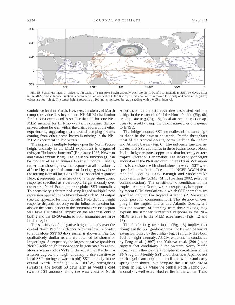
FIG. 15. Sensitivity map, or influence function, of a negative height anomaly over the North Pacific to anomalous SSTs 60 days earlierin the MLM. The influence function is contoured at an interval of 0.002 K m21; the zero contour is removed for clarity and positive (negative)values are red (blue). The target height response at 200 mb is indicated by gray shading with a 0.25-m interval.

confidence level in March. However, the observed Marchcomposite value lies beyond the NP–MLM distributionfor La Nina events and is smaller than all but one NP–MLM member for El Nino events. In contrast, the ob-served values lie well within the distributions of the otherexperiments, suggesting that a crucial damping processcoming from other ocean basins is missing in the NP–MLM experiment in late winter.

The impact of multiple bridges upon the North Pacificheight anomaly in the MLM experiment is diagnosedusing an ‘‘influence function’’ (Branstator 1985; Newmanand Sardeshmukh 1998). The influence function (g) canbe thought of as an inverse Green’s function. That is,rather than showing how the response at all locations isaffected by a specified source of forcing, g shows howthe forcing from all locations affects a specified response.Here, g represents the sensitivity of a target atmosphericresponse, specified as a barotropic height anomaly overthe central North Pacific, to prior global SST anomalies.This sensitivity is determined using lagged multiple linearregression applied to the November–March MLM output(see the appendix for more details). Note that the heightresponse depends not only on the influence function butalso on the actual pattern of the anomalous SSTs: a regionwill have a substantial impact on the response only ifboth g and the ENSO-induced SST anomalies are largein that region.

The sensitivity of a negative height anomaly over thecentral North Pacific (a deeper Aleutian low) in winterto anomalous SST 60 days earlier is shown in Fig. 15;qualitatively similar results are obtained for shorter orlonger lags. As expected, the largest negative (positive)North Pacific height response can be generated by anom-alously warm (cold) SSTs in the equatorial Pacific. Toa lesser degree, the height anomaly is also sensitive tolocal SST forcing: a warm (cold) SST anomaly in thecentral North Pacific (;358N, 1608W) strengthens(weakens) the trough 60 days later, as would a cold(warm) SST anomaly along the west coast of North

America. Since the SST anomalies associated with thebridge in the eastern half of the North Pacific (Fig. 6b)are opposite to g (Fig. 15), local air–sea interaction ap-pears to weakly damp the direct atmospheric responseto ENSO.

The bridge induces SST anomalies of the same signas those in the eastern equatorial Pacific throughoutmost of the tropical oceans, particularly in the Indianand Atlantic basins (Fig. 6). The influence function in-dicates that SST anomalies in these basins force a NorthPacific height response opposite to that forced by easterntropical Pacific SST anomalies. The sensitivity of heightanomalies in the PNA sector to Indian Ocean SST anom-alies is consistent with simulations in which SST werespecified in the Indian Ocean in the NCEP AGCM (Ku-mar and Hoerling 1998; Barsugli and Sardeshmukh2002) and in the CCM3 (M. P. Hoerling 2002, personalcommunication). The sensitivity to conditions in thetropical Atlantic Ocean, while unexpected, is supportedby recent CCM simulations in which SST anomalies arespecified only in the tropical Atlantic (R. Saravanan2002, personal communication). The absence of cou-pling in the tropical Indian and Atlantic Oceans, andthus the absence of damping from these regions, mayexplain the stronger wintertime response in the NP–MLM relative to the MLM experiment (Figs. 12 and13).

The dipole in g near Japan (Fig. 15) implies thatchanges in the SST gradient across the Kuroshio Currentextension forced by the bridge (Fig. 6) amplify the NorthPacific height anomaly. AGCM experiments conductedby Peng et al. (1997) and Yulaeva et al. (2001) alsosuggest that conditions in the western North PacificOcean can influence the atmospheric circulation in thePNA region. Monthly SST anomalies near Japan do notreach significant amplitude until late winter and earlyspring (not shown, but compare the DJF and MAMpanels in Fig. 6), while the central North Pacific SSTanomaly is well established earlier in the winter. Thus,


the net feedback from the Pacific north of 218N couldresult in damping of the height anomaly during mid-winter, but weaker damping and perhaps even amplifi-cation by late winter and early spring, which is consis-tent with the differences between the NP–MLM andcontrol experiments (and to a lesser degree the MLMand control) in Figs. 12 and 13. Note that the relation-ship between anomalous SST and the atmosphericheight anomalies also exhibits month-to-month varia-tions (Newman and Sardeshmukh 1998; Wang and Fu2000) not considered here.

c. Discussion

Our results suggest that the impact of air–sea couplingon the extratropical atmospheric response to ENSO iscomplex. Both local and remote air–sea interaction in-fluence ENSO teleconnections over the PNA region andcoupling effects vary with the seasonal cycle. The neteffect of global coupling on the ENSO response in thePNA sector is smaller than both the ENSO signal forceddirectly from the eastern Pacific and internal atmo-spheric variability (Fig. 14), which implies that verylarge ensembles are needed to determine the full effectof air–sea interaction on the response to ENSO at sub-seasonal timescales (Sardeshmukh et al. 2000).

The net global effect of coupling may be modest,however, because larger atmospheric responses to SSTanomalies in separate areas partly cancel over the PNAregion. Since the global SST anomaly pattern resultingfrom multiple bridges varies from event to event, thenet effect of coupling will also differ. Thus, to betterunderstand the full atmospheric response to ENSO andto simulate the response during individual ENSO eventswill require GCMs to correctly model a series of pro-cesses including: the SST evolution in the Indian, At-lantic, and North Pacific Oceans, the local atmosphericresponse to these SST anomalies, and the teleconnec-tions from these regions to the PNA sector.

Given the complexity of the model results, the phys-ical mechanisms responsible for the ocean-to-atmo-sphere feedback during ENSO events are not readilyapparent and likely involve both tropical and extratrop-ical processes. Air–sea interaction might influence theextratropical height response to ENSO via changes intropical precipitation. The warm 2 cold composite pre-cipitation in both coupled experiments minus the controlduring Feb(1) and the evolution of the precipitationanomalies in the central and western equatorial Pacificfor all three experiments are shown in Fig. 16. Couplingdecreases the tropical precipitation associated withENSO in midwinter by reducing the amplitude of pre-cipitation anomalies over the central and western equa-torial Pacific (Fig. 16c). Surprisingly, this signal is pre-sent even in the NP–MLM experiment, along with cor-responding changes in the 200-mb zonal winds (notshown), even though the SST boundary conditions south

of 208N are identical in the NP–MLM and control ex-periments.

The reduced precipitation in the central equatorialPacific in the coupled experiments during JF weakensthe diabatic forcing of the extratropical atmospheric cir-culation. The enhanced precipitation over 08–108N inthe Indian Ocean and the reduced precipitation near thePhilippines in the MLM relative to the NP–MLM (notshown but cf. Figs. 16a and 16b) are qualitatively similarto changes in the forcing necessary to further weakenthe extratropical wave train (e.g., Ting and Sardeshmukh1993). The difference in the precipitation/circulationover the tropical Pacific between the NP–MLM and con-trol experiments is unexpected and may be due to in-sufficient sampling. However, the difference betweenthe precipitation between the NP–MLM and control ex-periments is statistically significant in the central andwestern equatorial Pacific. Air–sea coupling in theNorth Pacific (including the subtropics) could influencetropical precipitation through processes that span fromthe midlatitudes to the Tropics, such as cold surges thatpropagate from Asia to the western equatorial Pacific.

In addition to changes in tropical forcing, differencesbetween the experiments may result from extratropicalprocesses. For example, reduced thermal damping couldcontribute to the enhancement of the NP–MLM re-sponse relative to the control in March. Indeed, the lossof energy from the atmosphere to the ocean via surfaceheat fluxes is 20%–30% weaker by February in the NP–MLM experiment (not shown, but see Figs. 4–12 in Lauand Nath 1996), consistent with the slow adjustment ofmidlatitude SST anomalies to the overlying atmosphere.However, the ENSO-related SST anomalies in the NorthPacific are also driven by anomalous low-level winds,which are not considered in the reduced thermal damp-ing paradigm. The sensitivity of central North Pacificheights to SST changes near Japan (Fig. 15) suggeststhat changes in the storm track could also be relevant.In March, precipitation just south of Japan and transienteddy flux convergence over the west Pacific are en-hanced in the NP–MLM relative to the control (notshown). While these differences in storm track param-eters are significant at the 99% and 95% levels, re-spectively, it is not yet clear whether the changes in thetransient eddies caused or resulted from the large-scalecirculation anomalies.

Finally, we note that one advantage of our experi-mental design compared to coupling an AGCM to anOGCM is that, by construction, SST anomalies are re-alistic in the ENSO region. Recent research (Pierce etal. 2000; Vimont et al. 2001), however, has suggestedthat winds in the extratropics may affect the develop-ment of tropical SST anomalies, a potentially importantfeedback missing from our experiments.

d. Oceanic feedback in other locations

While we have focused on the impact of air–sea in-teraction in the ENSO response in the PNA sector, air–


FIG. 16. (a) MLM minus control and (b) NP–MLM minus control warm 2 cold composite tropical precipitationduring Feb(1). Contour (shading) interval is 0.1 (0.05) cm day21. (c) Warm 2 cold composite of the 30-day runningmean precipitation (cm day21) in the MLM, NP–MLM, and control experiments averaged over the regions shown in(b): the central (58–158S, 1708E–1508W) and western (58S–58N, 1208–1608E) equatorial Pacific. Precipitation anomaliesin the central (western) Pacific are shown by solid (dashed) lines; open circles indicate that the differences betweenthe anomalies in the MLM or NP–MLM and the control are significant.

sea feedback influences the atmospheric bridge in otherregions as well. Wang et al. (2000) proposed that astrong anticyclone that forms to the east of the Philip-pines during El Nino winters creates cold SST anomaliesnear 108N, 1408E via evaporative cooling and enhancedentrainment. These cold SSTs reinforce the anticyclone,enabling it to persist for several months. By comparingthe local atmospheric response in a coupled and an un-coupled simulation, Lau and Nath (2000) found that theENSO-related SST anomalies in the Indian Ocean tendto enhance (reduce) the precipitation and flow in thesummer Asian monsoon, in opposition to the direct re-

sponse to warm (cold) SST anomalies in the tropicalPacific Ocean.

9. Outstanding issues

The full extent of the atmospheric bridge spans sev-eral different processes, including the following: theglobal atmospheric response to ENSO SST anomalies;the resulting changes in heat, momentum, and fresh-water fluxes across the air–sea interface outside of theequatorial Pacific; the ocean’s response to these surfaceflux anomalies, including changes in SST, MLD, and


salinity; and the feedback of the remote SST anomaliesonto the atmosphere. While considerable progress hasbeen made in our understanding of each of these sub-topics, several outstanding issues remain.

A detailed discussion of unresolved issues concerningthe atmospheric response to tropical SST anomalies canbe found in section 6 of Trenberth et al. (1998). Ofrelevance here is how the large-scale atmosphericchanges associated with ENSO are communicated to thesurface via changes in solar radiation, precipitation, andboundary layer processes, which are not well simulatedin AGCMs. Perhaps the most important requirement, interms of improved simulation of the ENSO-related SSTanomalies, is a better representation of clouds and theirinfluence on solar radiation.

Most studies that have examined the remote oceanicresponse to ENSO have focused on SST anomalies inthe Northern Hemisphere during winter. Relatively largeENSO-related SST anomalies in the Southern Hemi-sphere during winter and in the North Pacific duringsummer have received much less attention. Questionsalso remain about the Indian Ocean response to ENSO;while most studies have found a basinwide warming inDec(0)–May(1), it is not clear how much of the east–west SST dipole that develops along the equator in bo-real fall is also due to the atmospheric bridge. In ad-dition, the remote influence of ENSO on other oceanfields such as mixed layer depth, and temperature, sa-linity, and currents as a function of depth requires fur-ther study.

A complete picture of the climate system response toENSO should incorporate both the atmospheric bridgeand the dynamical ocean response to tropical SST anom-alies. Kelvin and other coastally trapped ocean wavesgenerated by ENSO clearly influence SST along thewest coast of North and South America. BaroclinicRossby waves are generated by the passage of thesewaves and by changes in wind stress curl associatedwith atmospheric teleconnections, especially variationsin the Aleutian low (Pares Siera and O’Brien 1989;Jacobs et al. 1994; Miller et al. 1997). Since baroclinicRossby waves take approximately 5–10 years to crossthe North Pacific, dynamical ocean processes are im-portant in slow basinwide thermocline changes and mayinfluence SST anomalies at low frequencies. Wind andbuoyancy driven changes in the ocean circulation mayalso result from the atmospheric response to low-fre-quency changes in SST in the equatorial Pacific. In prin-ciple, coupled GCMs can be used to assess the roles ofthe atmosphere and oceans in the global response toSST anomalies in the equatorial Pacific, provided themodels have a reasonable representation of ENSO.

Perhaps the most outstanding issue concerning theatmospheric bridge is the extent to which and by whatmeans SST anomalies beyond the equatorial east Pacificfeed back on the atmosphere. The effect of midlatitudeair–sea feedback on the atmospheric circulation duringENSO has differed among previous modeling studies.

The GCM simulations we have performed suggest thatglobal air–sea interaction damps the midwinter responseto ENSO in the PNA region while air–sea interactionin the North Pacific strengthens the response in March.However, several questions remain. Are both signalsrobust and reproducible in other models? If so, whatphysical processes are responsible? Is reduced thermaldamping, which enhances persistence of atmosphericanomalies (e.g., Barsugli and Battisti 1998) critical, and/or are dynamical changes, perhaps a change in the in-tensity or location of the storm tracks, important as well?How does air–sea interaction, including interactions inthe North Pacific, influence tropical precipitation? Doesreemergence of ENSO-related SST anomalies in the fol-lowing fall/winter affect the atmosphere? How does air–sea interaction during ENSO in other locations, for ex-ample, the tropical Atlantic, Indian Ocean, and SouthernHemisphere influence the atmospheric response toENSO? More definitive answers to these questions re-quire a very large ensemble of coupled and uncoupledsimulations.

Acknowledgments. We thank Mary Jo Nath and Chris-topher Winkler for their assistance in analyzing andgraphing the results. Comments by Robert Scott andtwo anonymous reviewers along with conversationswith Gil Compo and Joe Barsugli helped to improve themanuscript. Tom Smith from NCEP provided the SSTsused as boundary conditions in the model simulations.

APPENDIX

Empirical Influence Functions

The linear evolution of an anomaly vector x(t) overa time interval [t, t 1 t] can be expressed as

x(t 1 t) 5 G(t)x(t) 1 s(t 1 t), (A1)

where G(t) is a linear operator (or propagator) matrixand s(t 1 t) is the corresponding error vector. Here G(t)can be determined from the zero-lag and time-lag cov-ariability statistics of x(t) in a least squares sense (e.g.,Wilks 1995) using multiple linear regression (MLR).Now suppose we are interested in a particular patternof the response to prior anomalous initial conditions,say the height anomaly over the North Pacific that re-sults from anomalous SST forcing 60 days earlier. Letw be a vector that represents this response of interest.Then a measure of the magnitude of this response is theprojection of w on the total field x(t 1 t), or

TR 5 w x(t 1 t). (A2)

From (A1) and (A2) the expected response for a giveninitial state x(t) is

T^R& 5 w G(t)x(t), (A3)

where the brackets indicate an ensemble average so that^s& 5 0. Thus, the sensitivity of the response w to initial


conditions in any location can be determined from (A3)as

T Tg 5 w G(t). (A4)

An element of this sensitivity map, or influence functiong(u, l), is the contribution to the target response froma point with unit initial condition located at latitude uand longitude l.

The influence function shares two notable similaritieswith the Green’s function. First, convolving g with anactual pattern of SST forcing at any given time willproduce a corresponding height response. Second, gmeasures the cumulative effect of forcing over the timeinterval t. For example, a point source of anomalousSST in the Tropics may directly produce a North Pacificheight response, but it may also induce anomalous SSTin other locations that could in turn further enhance orreduce the height anomaly.

In this analysis, we apply MLR to the anomaly vectordefined as

T x 5 Z , 850 Z200

where T is the anomalous SST subvector, and Z200 andZ850 are 200- and 850-mb geopotential height anomalysubvectors. Data north of 308S are interpolated to a 583 58 grid. Anomalies are determined during NDJFM asdepartures of daily values from an annually varyingclimatology, where the climatology is defined as botha time and ensemble mean. Anomalies are then filteredwith a 30-day running mean. Finally, anomalies are trun-cated in EOF space to the 40 leading geopotential heightand SST EOFs. This truncation retains more than 80%of domain-integrated variance for each field. A lag of20 days is used to compute G(t), as G(t) 5

Results are not qualitatively sensitive to ei-t/20[G(20)] .ther truncation or lag. Apart from sampling, results arealso similar if we compute (t) from other lags; forGexample, suggesting3 2G(60) 5 [G(20)] 5 [G(30)] ,that the evolution of x can be described by a simplelinear dynamical equation (Winkler et al. 2001). Sincethe influence function in Fig. 15 shows sensitivity of aheight response alone, the SST subvector of w is set tozero. In addition, only the SST portion of g is shownin Fig. 15, but similar maps result at 200 and 850 mbfor the sensitivity of the North Pacific height anomalyto previous height anomalies.

REFERENCES

Alexander, M. A., 1990: Simulation of the response of the NorthPacific Ocean to the anomalous atmospheric circulation asso-ciated with El Nino. Climate Dyn., 5, 53–65.

——, 1992a: Midlatitude atmosphere–ocean interaction during ElNino. Part I: The North Pacific Ocean. J. Climate, 5, 944–958.

——, 1992b: Midlatitude atmosphere–ocean interaction during ElNino. Part II: The North Hemisphere atmosphere. J. Climate, 5,959–972.

——, and C. Deser, 1995: A mechanism for the recurrence of win-tertime midlatitude SST anomalies. J. Phys. Oceanogr., 25, 122–137.

——, and J. D. Scott, 1995: Atlas of climatology and variability inthe GFDL R30S14 GCM. CIRES, University of Colorado, 121pp. [Available from the authors at NOAA–CIRES Climate Di-agnostics Center, R/CDC1, 325 Broadway, Boulder, CO 80305-3328.]

——, and ——, 1997: Surface flux variability over the North Pacificand North Atlantic Oceans. J. Climate, 10, 2963–2978.

——, C. Deser, and M. S. Timlin, 1999: The reemergence of SSTanomalies in the North Pacific Ocean. J. Climate, 12, 2419–2433.

——, J. D. Scott, and C. Deser, 2000: Processes that influence seasurface temperature and ocean mixed layer depth variability ina coupled model. J. Geophys. Res., 105, 16 823–16 842.

——, M. S. Timlin, and J. D. Scott, 2001: Winter-to-winter recurrenceof sea surface temperature, salinity and mixed layer depth anom-alies. Progress in Oceanography, Vol. 49, Pergamon, 41–61.

Barsugli, J. J., 1995: Idealized models of intrinsic midlatitude at-mosphere–ocean interaction. Ph.D. thesis, University of Wash-ington, 187 pp. [Available online at http://www.cdc.noaa.gov/;jjb/thesis.html.]

——, and D. S. Battisti, 1998: The basic effects of atmosphere–oceanthermal coupling on midlatitude variability. J. Atmos. Sci., 55,477–493.

——, and P. D. Sardeshmukh, 2002: Global atmospheric sensitivityto tropical SST anomalies throughout the Indo-Pacific basin. J.Climate, in press.

Behera, S. K., P. S. Salvekar, and T. Yamagata, 2000: Simulation ofinterannual SST variability in the tropical Indian Ocean. J. Cli-mate, 13, 3487–3499.

Bhatt, U. S., M. A. Alexander, D. S. Battisti, D. D. Houghton, andL. M. Keller, 1998: Atmosphere–ocean interaction in the NorthAtlantic: Near-surface climate variability. J. Climate, 11, 1615–1632.

Bjerknes, J., 1966: A possible response of the atmospheric Hadleycirculation to equatorial anomalies of ocean temperatures. Tellus,18, 820–829.

——, 1969: Atmospheric teleconnections from the equatorial Pacific.Mon. Wea. Rev., 97, 163–172.

Blackmon, M. L., J. E. Geisler, and E. J. Pitcher, 1983: A generalcirculation model study of January climate anomaly patternsassociated with interannual variation of equatorial Pacific seasurface temperatures. J. Atmos. Sci., 40, 1410–1425.

Blade, I., 1997: The influence of midlatitude ocean–atmosphere cou-pling on the low-frequency variability of a GCM. Part I: Notropical SST forcing. J. Climate, 10, 2087–2106.

——, 1999: The influence of midlatitude ocean–atmosphere couplingon the low-frequency variability of a GCM. Part II: Interannualvariability induced by tropical SST forcing. J. Climate, 12, 21–45.

Branstator, G., 1985: Analysis of general circulation model sea-sur-face temperature anomaly simulations using a linear model. PartI: Forced solutions. J. Atmos. Sci., 42, 2225–2241.

Broccoli, A. J., and S. Manabe, 1992: The effects of orography onmidlatitude Northern Hemisphere dry climates. J. Climate, 5,1181–1201.

Cadet, D. L., 1985: The Southern Oscillation over the Indian Ocean.Int. J. Climatol., 5, 189–212.

Cayan, D. R., 1990: Variability of latent and sensible heat flux overthe oceans. Ph.D. thesis, University of California, San Diego,199 pp.

Chambers, D. P., B. D. Tarpley, and R. H. Stewart, 1999: Anomalouswarming in the Indian Ocean coincident with El Nino. J. Geo-phys. Res., 104, 3035–3047.

Collins, J. A., J. D. Scott, C. A. Smith, and M. A. Alexander, 2001:The GFDL Electronic Climate Atlas. [Available online athttp://www.cdc.noaa.gov/gfdl.]


Covey, D. L., and S. Hastenrath, 1978: The Pacific El Nino phenom-enon in the Atlantic sector. Mon. Wea. Rev., 106, 1280–1287.

Curtis, S., and S. Hastenrath, 1995: Forcing of anomalous sea surfacetemperature evolution in the tropical Atlantic during Pacificwarm events. J. Geophys. Res., 100, 15 835–15 847.

Dayton, P. K., and M. J. Tegner, 1990: Bottoms beneath troubledwaters: Benthic impacts of the 1982–1984 El Nino in the tem-perate zone. Global Ecological Consequences of the 1982–83El Nino–Southern Oscillation, P. W. Glynn, Ed., Elsevier, 433–472.

Deser, C., and M. L. Blackmon, 1995: On the relationship betweentropical and North Pacific sea surface temperature variations. J.Climate, 8, 1677–1680.

——, M. A. Alexander, and M. S. Timlin, 1996: Upper-ocean thermalvariations in the North Pacific during 1970–1991. J. Climate, 9,1841–1855.

Emery, W. J., and K. Hamilton, 1985: Atmospheric forcing of inter-annual variability in the northeast Pacific Ocean: Connectionswith El Nino. J. Geophys. Res., 90, 857–868.

Enfield, D. B., and D. A. Mayer, 1997: Tropical Atlantic sea surfacetemperature variability and its relation to El Nino–Southern Os-cillation. J. Geophys. Res., 102, 929–945.

——, and A. M. Mestas-Nunez, 1999: Multiscale variabilities in glob-al sea surface temperatures and their relationships with tropo-spheric climate patterns. J. Climate, 12, 2719–2733.

Ferranti, L., F. Molteni, and T. N. Palmer, 1994: Impact of localizedtropical and extratropical SST anomalies in ensembles of sea-sonal GCM integrations. Quart. J. Roy. Meteor. Soc., 120, 1613–1645.

Frankignoul, C., 1985: Sea surface temperature anomalies, planetarywaves, and air–sea feedback in the middle latitudes. Rev. Geo-phys., 23, 357–390.

——, and R. W. Reynolds, 1983: Testing a dynamical model formidlatitude sea surface temperature anomalies. J. Phys. Ocean-ogr., 13, 1131–1145.

Garreaud, R. D., and D. S. Battisti, 1999: Interannual (ENSO) andinterdecadal (ENSO-like) variability in the Southern Hemispheretropospheric circulation. J. Climate, 12, 2113–2123.

Gaspar, P., 1988: Modeling the seasonal cycle of the upper ocean. J.Phys. Oceanogr., 18, 161–180.

Giannini, A., Y. Kushnir, and M. A. Cane, 2000: Interannual vari-ability of Caribbean rainfall, ENSO, and the Atlantic Ocean. J.Climate, 13, 297–311.

Gill, A. E., 1980: Some simple solutions for heat-induced tropicalcirculation. Quart. J. Roy. Meteor. Soc., 106, 447–462.

Gordon, C. T., and W. Stern, 1982: A description of the GFDL globalspectral model. Mon. Wea. Rev., 110, 625–644.

Graham, N. E., T. P. Barnett, R. Wilde, M. Ponater, and S. Scuhbert,1994: On the roles of tropical and midlatitude SSTs in forcingannual to interdecadal variability in the winter Northern Hemi-sphere circulation. J. Climate, 7, 1416–1442.

Gu, D., and S. G. H. Philander, 1997: Interdecadal climate fluctuationsthat depend on exchanges between the tropics and extratropics.Science, 275, 805–807.

Hanawa, K. T., T. Watanabe, N. Iwasaka, and T. Suga, 1988: Surfacethermal conditions in the western North Pacific during the ENSOevents. J. Meteor. Soc. Japan, 66, 445–456.

——, Y. Yoshikawa, and T. Watanabe, 1989: Composite analyses ofwintertime wind stress vector fields with respect to SST anom-alies in the western North Pacific and the ENSO events. Part I:SST composite. J. Meteor. Soc. Japan, 67, 385–400.

Harrison, D. E., and N. K. Larkin, 1998: El Nino–Southern Oscillationsea surface temperature and wind anomalies. Rev. Geophys., 36,353–399.

Hastenrath, S., L. C. Castro, and P. Aceituno, 1987: The SouthernOscillation in the Atlantic sector. Contrib. Atmos. Phys., 60, 447–463.

Held, I. M., S. W. Lyons, and S. Nigam, 1989: Transients and theextratropical response to El Nino. J. Atmos. Sci., 46, 163–174.

Hendon, H. H., and D. L. Hartmann, 1982: Stationary waves on a

sphere: Sensitivity to thermal feedback. J. Atmos. Sci., 39, 1906–1920.

Hoerling, M. P., and A. Kumar, 2002: Atmospheric response patternsassociated with tropical forcing. J. Climate, 15, 2184–2203.

Horel, J. D., and J. M. Wallace, 1981: Planetary-scale atmosphericphenomena associated with the interannual variability of seasurface temperature in the equatorial Pacific. Mon. Wea. Rev.,109, 813–829.

Hoskins, B. J., and D. J. Karoly, 1981: The steady linear responseof a spherical atmosphere to thermal and orographic forcing. J.Atmos. Sci., 38, 1179–1196.

Hsiung, J., and R. E. Newell, 1983: The principal nonseasonal modesof variation of global sea surface temperature. J. Phys. Ocean-ogr., 13, 1957–1967.

Iwasaka, N., and J. M. Wallace, 1995: Large scale air sea interactionin the Northern Hemisphere from a view point of variations ofsurface heat flux by SVD analysis. J. Meteor. Soc. Japan, 73,781–794.

Jacobs, G. A., H. E. Hurlburt, J. C. Kindle, E. J. Metzger, J. L.Mitchell, and A. J. Wallcraft, 1994: Decade-scale trans-Pacificpropagation and warming effects of an El Nino anomaly. Nature,370, 360–363.

Johnson, M. A., and J. J. O’Brien, 1990: The northeast Pacific Oceanresponse to the 1982–1983 El Nino. J. Geophys. Res., 95, 7155–7166.

Kalnay, E., and Coauthors, 1996: The NCEP/NCAR 40-Year Re-analysis Project. Bull. Amer. Meteor. Soc., 77, 437–471.

Kawamura, R., 1994: A rotated EOF analysis of global sea surfacetemperature variability with interannual and interdecadal scales.J. Phys. Oceanogr., 24, 707–715.

Kendall, M., and A. Stuart, 1977: The Advanced Theory of Statistics.3d ed. Vol. 1, Macmillian, 283 pp.

Kiladis, G. N., and H. F. Diaz, 1989: Global climate anomalies as-sociated with extremes in the Southern Oscillation. J. Climate,2, 1069–1090.

Kistler, R., and Coauthors, 2001: The NCEP–NCAR 50-Year Re-analysis: Monthly means CD-ROM and documentation. Bull.Amer. Meteor. Soc., 82, 247–267.

Klein, S. A., B. J. Soden, and N.-C. Lau, 1999: Remote sea surfacevariations during ENSO: Evidence for a tropical atmosphericbridge. J. Climate, 12, 917–932.

Kok, C. J., and J. D. Opsteegh, 1985: Possible causes of anomaliesin seasonal mean circulation patterns during the 1982–83 El Ninoevent. J. Atmos. Sci., 42, 677–694.

Kumar, A., and M. P. Hoerling, 1995: Prospects and limitations ofseasonal atmospheric GCM predictions. Bull. Amer. Meteor.Soc., 76, 335–345.

——, and ——, 1998: Specification of regional sea surface temper-atures in atmospheric general circulation model simulations. J.Geophys. Res., 103, 8901–8907.

Kushnir, Y., W. A. Robinson, I. Blade, N. M. J. Hall, S. Peng, andR. Sutton, 2002: Atmospheric GCM response to extratropicalSST anomalies: Synthesis and evaluation. J. Climate, 15, 2233–2256.

Lanzante, J., 1996: Lag relationships involving tropical sea surfacetemperatures. J. Climate, 9, 2568–2578.

Latif, M., 2000: Tropical Pacific/Atlantic Ocean interactions at multi-decadal time scales. Max Planck Institute Rep. 305, Hamburg,Germany, 13 pp.

——, and T. P. Barnett, 1994: Causes of decadal climate variabilityover the North Pacific and North America. Science, 266, 634–637.

——, and ——, 1995: Interactions of the tropical oceans. J. Climate,8, 952–964.

——, and ——, 1996: Decadal climate variability over the NorthPacific and North America: Dynamics and predictability. J. Cli-mate, 9, 2407–2423.

——, E. Roeckner, U. Mikolajewivz, and R. Voss, 2000: Tropicalstabilization of the thermohaline circulation in a greenhousewarming. J. Climate, 13, 1809–1813.


Lau, N.-C., 1997: Interactions between global SST anomalies and themidlatitude atmospheric circulation. Bull. Amer. Meteor. Soc.,78, 21–33.

——, and M. J. Nath, 1994: A modeling study of the relative rolesof tropical and extratropical SST anomalies in the variability ofthe global atmosphere–ocean system. J. Climate, 7, 1184–1207.

——, and ——, 1996: The role of the ‘‘atmospheric bridge’’ in linkingtropical Pacific ENSO events to extratropical SST anomalies. J.Climate, 9, 2036–2057.

——, and ——, 2000: Impact of ENSO on the variability of theAsian–Australian monsoons as simulated in GCM experiments.J. Climate, 13, 4287–4309.

——, and ——, 2001: Impact of ENSO on SST variability in theNorth Pacific and North Atlantic: Seasonal dependence and roleof extratropical air–sea coupling. J. Climate, 14, 2846–2866.

Lockyer, N., and W. J. S. Lockyer, 1902: On the similarity of theshort-period pressure variations over large areas. Proc. Roy. Soc.London, 71, 134–136.

Lukas, R., and E. Lindstrom, 1991: The mixed layer of the westernequatorial Pacific Ocean. J. Geophys. Res., 96, 3343–3357.

Luksch, U., and H. von Storch, 1992: Modeling the low-frequencysea surface temperature variability in the North Pacific. J. Cli-mate, 5, 893–906.

——, ——, and E. Maier-Reimer, 1990: Modeling North Pacific SSTanomalies as a response to anomalous atmospheric forcing. J.Mar. Syst., 1, 51–60.

Manabe, S., and R. J. Stouffer, 1996: Low-frequency variability ofsurface air temperature in a 1000-year integration of a coupledatmosphere–ocean–land surface model. J. Climate, 9, 376–393.

Mantua, N. J., S. R. Hare, Y. Zhang, J. M. Wallace, and R. Francis,1997: A Pacific interdecadal climate oscillation with impacts onsalmon production. Bull. Amer. Meteor. Soc., 78, 1069–1079.

Matsuno, T., 1966: Quasi-geostrophic motions in the equatorial area.J. Meteor. Soc. Japan, 44, 25–43.

Mestas-Nunez, A. M., and D. B. Enfield, 1999: Rotated global modesof non-ENSO sea surface temperature variability. J. Climate, 12,2734–2746.

Miller, A. J., and N. Schneider, 2000: Interdecadal climate regimedynamics in the North Pacific Ocean: Theories, observations,and ecosystem impacts. Progress in Oceanography, Vol. 47,Pergamon, 355–379.

——, D. R. Cayan, T. P. Barnett, N. E. Graham, and J. M. Oberhuber,1994: Interdecadal variability of the Pacific Ocean: Model re-sponse to observed heat flux and wind stress anomalies. ClimateDyn., 10, 287–302.

——, W. B. White, and D. R. Cayan, 1997: North Pacific thermoclinevariations on ENSO timescales. J. Phys. Oceanogr., 27, 2023–2039.

Monterey, G. I., and S. Levitus, 1997: Climatological cycle of mixedlayer depth in the world ocean. NOAA/NESDIS, U.S. Govt.Printing Office, 5 pp.

Moron, V., R. Vautard, and M. Ghil, 1998: Trends, interdecadal andinterannual oscillations in global sea-surface temperatures. Cli-mate Dyn., 14, 545–569.

Murtugudde, R., and A. Busalachi, 1999: Interannual variability ofthe dynamics and thermodynamics of the tropical Indian Ocean.J. Climate, 12, 2300–2326.

Mysak, L. A., 1986: El Nino, interannual variability and fisheries inthe northeast Pacific Ocean. Can. J. Fish. Aquat. Sci., 43, 464–497.

Nakamura, H., G. Lin, and T. Yamagata, 1997: Decadal climate var-iability in the North Pacific in recent decades. Bull. Amer. Me-teor. Soc., 78, 2215–2226.

Namias, J., 1976: Some statistical and synoptic characteristics as-sociated with El Nino. J. Phys. Oceanogr., 6, 130–138.

——, and R. M. Born, 1970: Temporal coherence in North Pacificsea-surface temperature patterns. J. Geophys. Res., 75, 5952–5955.

——, and ——, 1974: Further studies of temporal coherence in NorthPacific sea surface temperatures. J. Geophys. Res., 79, 797–798.

Newman, M., and P. D. Sardeshmukh, 1998: The impact of the annualcycle on the North Pacific/North American response to remotelow-frequency forcing. J. Atmos. Sci., 55, 1336–1353.

——, M. A. Alexander, C. R. Winkler, J. D. Scott, and J. J. Barsugli,2000: A linear diagnosis of the coupled extratropical ocean–atmosphere system in the GFDL GCM. Atmos. Sci. Lett., 1, 14–25.

Nicholson, S. E., 1997: An analysis of the ENSO signal in the tropicalAtlantic and western Indian Oceans. Int. J. Climatol., 17, 345–375.

Niebauer, H. J., 1984: On the effect of El Nino events in Alaskanwaters. Bull. Amer. Meteor. Soc., 65, 472–473.

——, 1988: Effects of El Nino–Southern Oscillation and North Pa-cific weather patterns on interannual variability in the southernBering Sea. J. Geophys. Res., 93, 5051–5068.

Nitta, T., and S. Yamada, 1989: Recent warming of tropical sea sur-face temperature and its relationship to the Northern Hemispherecirculation. J. Meteor. Soc. Japan, 67, 375–383.

Pan, Y. H., and A. H. Oort, 1983: Global climate variations connectedwith sea surface temperature anomalies in the eastern equatorialPacific Ocean for the 1958–73 period. Mon. Wea. Rev., 111,1244–1258.

——, and ——, 1990: Correlation analyses between sea surface tem-perature anomalies in the eastern equatorial Pacific and the worldocean. Climate Dyn., 4, 191–205.

Pares-Sierra, A., and J. J. O’Brien, 1989: The seasonal and interannualvariability of the California Current System: A numerical model.J. Geophys. Res., 94, 3159–3180.

Peng, S., W. A. Robinson, and M. P. Hoerling, 1997: The modeledatmospheric response to midlatitude SST anomalies and its de-pendence on background circulation states. J. Climate, 10, 971–987.

Penland, C., and P. D. Sardeshmukh, 1995: The optimal growth oftropical sea surface temperature anomalies. J. Climate, 8, 1999–2024.

——, and L. Matrosova, 1998: Prediction of tropical Atlantic seasurface temperatures using linear inverse modeling. J. Climate,11, 483–496.

Pierce, D. W., T. P. Barnett, and M. Latif, 2000: Connections betweenthe Pacific Ocean Tropics and midlatitudes on decadal time-scales. J. Climate, 13, 1173–1194.

Polovina, J. J., G. T. Mitchum, and G. T. Evans, 1995: Decadal andbasin-scale variation in mixed layer depth and the impact onbiological production in the central and North Pacific, 1960–88.Deep-Sea Res., 42, 1701–1716.

Qiu, B., 2000: Interannual variability of the Kuroshio extension sys-tem and its impact on the wintertime SST field. J. Phys. Ocean-ogr., 30, 1486–1502.

Rasmusson, E. M., and T. H. Carpenter, 1982: Variations in tropicalsea surface temperature and surface wind fields associated withthe Southern Oscillation/El Nino. Mon. Wea. Rev., 110, 354–384.

Reynolds, R. W., and E. M. Rasmusson, 1983: The North Pacific seasurface temperature associated with El Nino events. Proc. Sev-enth Annual Climate Diagnostics Workshop, Boulder, CO,NOAA/NCEP/CPC, 298–310. [NTIS PB283-208033.]

——, and T. M. Smith, 1994: Improved global sea surface temperatureanalyses using optimum interpolation. J. Climate, 7, 929–948.

Rienecker, M. M., and C. N. K. Mooers, 1986: The 1982–1983 ElNino signal off northern California. J. Geophys. Res., 91, 6597–6608.

Robinson, W. A., 2000: Review of WETS—The Workshop on Extra-Tropical SST Anomalies. Bull. Amer. Meteor. Soc., 81, 567–577.

Rodwell, M. J., D. P. Rowell, and C. K. Folland, 1999: Oceanicforcing of the wintertime North Atlantic Oscillation and Euro-pean climate. Nature, 398, 320–323.

Ropelewski, C. F., and M. S. Halpert, 1987: Global and regional scaleprecipitation patterns associated with the El Nino/Southern Os-cillation. Mon. Wea. Rev., 115, 1606–1626.

Rowntree, P. R., 1972: The influence of tropical east Pacific Ocean


temperatures on the atmosphere. Quart. J. Roy. Meteor. Soc.,98, 290–321.

Saji, N. H., B. N. Goswami, P. N. Vinayachandran, and T. Yamagata,1999: A dipole mode in the tropical Indian Ocean. Nature, 401,360–363.

Saravanan, R., 1998: Atmospheric low frequency variability and itsrelationship to midlatitude SST variability: Studies using theNCAR Climate System Model. J. Climate, 11, 1386–1404.

——, and P. Chang, 2000: Interaction between tropical Atlantic var-iability and El Nino–Southern Oscillation. J. Climate, 13, 2177–2194.

Sardeshmukh, P. D., and B. J. Hoskins, 1988: The generation of globalrotational flow by steady, idealized tropical divergence. J. Atmos.Sci., 45, 1228–1251.

——, G. P. Compo, and C. Penland, 2000: Changes of probabilityassociated with El Nino. J. Climate, 13, 4268–4286.

Schmittner, A., C. Appenzeller, and T. F. Stocker, 2000: EnhancedAtlantic freshwater export during El Nino. Geophys. Res. Lett.,27, 1163–1666.

Scott, J. D., and M. A. Alexander, 1999: Net shortwave fluxes overthe ocean. J. Phys. Oceanogr., 29, 3167–3174.

Simmons, A. J., J. M. Wallace, and G. W. Branstator, 1983: Barotropicwave propagation and instability, and atmospheric teleconnec-tion patterns. J. Atmos. Sci., 40, 1363–1392.

Simpson, J. J., 1983: Large scale thermal anomalies in the Californiacurrent during the 1982–83 El Nino. Geophys. Res. Lett., 10,937–940.

Smith, T. M., R. W. Reynolds, R. E. Livezey, and D. C. Stokes, 1996:Reconstruction of historical sea surface temperatures using em-pirical orthogonal functions. J. Climate, 9, 1403–1420.

Ting, M., and P. D. Sardeshmukh, 1993: Factors determining theextratropical response to equatorial diabatic heating anomalies.J. Atmos. Sci., 50, 907–918.

——, and S. Peng, 1995: Dynamics of early and midwinter responsesto the northwest Atlantic SST anomalies. J. Climate, 8, 2239–2254.

Tourre, Y. M., and W. B. White, 1995: ENSO signals in global upper-ocean temperature. J. Phys. Oceanogr., 25, 1317–1332.

Trenberth, K. E., 1997: The definition of El Nino. Bull. Amer. Meteor.Soc., 78, 2771–2778.

——, and J. D. A. Paolino, 1981: Characteristic patterns of variabilityof sea level pressure in the Northern Hemisphere. Mon. Wea.Rev., 109, 1169–1189.

——, and J. W. Hurrell, 1994: Decadal atmosphere–ocean variationsin the Pacific. Climate Dyn., 9, 303–319.

——, G. W. Branstator, D. Karoly, A. Kumar, N.-C. Lau, and C.Ropelewski, 1998: Progress during TOGA in understanding andmodeling global teleconnections associated with tropical sea sur-face temperatures. J. Geophys. Res., 103, 14 291–14 324.

Uvo, C. B., C. A. Repelli, S. E. Zebiak, and Y. Kushnir, 1998: Therelationships between tropical Pacific and Atlantic SST andnortheast Brazil monthly precipitation. J. Climate, 11, 551–561.

van Loon, H., and R. A. Madden, 1981: The Southern Oscillation.Part I. Global associations with pressure and temperature innorthern winter. Mon. Wea. Rev., 109, 1150–1162.

Venzke, S., M. Latif, and A. Villwock, 2000: The coupled GCMECHO-2. Part II: Indian Ocean response to ENSO. J. Climate,13, 1384–1405.

Vimont, D. J., D. S. Battisti, and A. C. Hirst, 2001: Footprinting: Aseasonal connection between the tropics and mid-latitudes. Geo-phys. Res. Lett., 28, 3923–3926.

Wagner, A. J., 1984: Possible mid-latitude atmospheric generation ofanomalously warm surface waters in the Gulf of Alaska fromautumn 1982 to spring 1983. Tropical Ocean–Atmosphere News-letter, No. 26, 15–16.

Walker, G. T., 1909: Correlation in seasonal variation of climate. Mem.India Meteor. Dept., 20, 117–124.

——, 1924: Correlation in seasonal variations of weather IX. Mem.India Meteor. Dept., 24, 275–332.

——, and E. W. Bliss, 1932: World Weather V. Mem. Roy. Meteor.Soc., 4, 53–84.

Wallace, J. M., and Q. Jiang, 1987: On the observed structure of theinterannual variability of the atmosphere/ocean climate system.Atmospheric and Oceanic Variability, H. Cattle, Ed., Royal Me-teorological Society, 17–43.

——, E. M. Rasmusson, T. P. Mitchell, V. E. Kousky, E. S. Sarachik,and H. von Storch, 1998: On the structure and evolution ofENSO-related climate variability in the tropical Pacific: Lessonsfrom TOGA. J. Geophys. Res., 103, 14 241–14 260.

Wang, B., R. Wu, and X. Fu, 2000: Pacific–East Asian teleconnection:How does ENSO affect east Asian climate. J. Climate, 13, 1517–1536.

Wang, H., and R. Fu, 2000: Winter monthly mean atmospheric anom-alies over the North Pacific and North America associated withEl Nino SSTs. J. Climate, 13, 3435–3447.

Watanabe, M., and M. Kimoto, 2000: On the persistence of decadalSST anomalies in the North Atlantic. J. Climate, 13, 3017–3028.

Weare, B. C., A. R. Navato, and R. E. Newell, 1976: Empiricalorthogonal analysis of Pacific Ocean sea surface temperatures.J. Phys. Oceanogr., 6, 671–678.

Webster, P. J., A. M. Moore, J. P. Loschnig, and R. R. Leben, 1999:Coupled ocean–atmosphere dynamics in the Indian Ocean during1997–98. Nature, 401, 356–360.

White, W. B., 1995: Design of a global observing system for gyre-scale upper ocean temperature variability. Progress in Ocean-ography, Vol. 36, Pergamon, 169–217.

Wilks, D. S., 1995: Statistical Methods in the Atmospheric Sciences.Academic Press, 467 pp.

Winkler, C. R., M. Newman, and P. D. Sardeshmukh, 2001: A linearmodel of wintertime low-frequency variability. Part I: Formu-lation and forecast skill. J. Climate, 14, 4474–4494.

Wolter, K., 1987: The Southern Oscillation in surface circulation andclimate over the tropical Atlantic, eastern Pacific, and IndianOceans as captured by cluster analysis. J. Climate Appl. Meteor.,26, 540–541.

——, 1989: Modes of tropical circulation, Southern Oscillation, andSahel rainfall anomalies. J. Climate, 2, 149–172.

Wright, P. B., 1983: Sea surface temperature fluctuations in the Pa-cific, 08–508N. Tropical Ocean–Atmosphere Newsletter, No. 19,14–15.

Xie, P., and P. A. Arkin, 1997: Global precipitation: A 17-year month-ly analysis based on gauge observations, satellite estimates, andnumerical model outputs. Bull. Amer. Meteor. Soc., 78, 2539–2558.

Yasunari, T., 1987: Global structure of the El Nino/Southern Oscil-lation. Part I. El Nino composites. J. Meteor. Soc. Japan, 65,67–79.

Yu, L., and M. M. Rienecker, 1999: Mechanisms for the Indian Oceanwarming during the 1997–1998 El Nino. Geophys. Res. Lett.,26, 735–738.

Yulaeva, E., N. Schneider, D. W. Pierce, and T. P. Barnett, 2001:Modeling of North Pacific climate variability forced by oceanicheat flux anomalies. J. Climate, 14, 4027–4046.

Zhang, X., J. Sheng, and A. Shabbar, 1998: Modes of interannualand interdecadal variability of Pacific SST. J. Climate, 11, 2556–2569.

Zhang, Y., and J. M. Wallace, 1996: Is climate variability over theNorth Pacific a linear response to ENSO? J. Climate, 9, 1468–1478.

——, ——, and D. S. Battisti, 1997: ENSO-like interdecadal vari-ability. J. Climate, 10, 1004–1020.

Zhao, Y. P., and G. A. McBean, 1986: Annual and interannual var-iability of the North Pacific ocean–atmosphere total heat transfer.Atmos.–Ocean, 24, 283–291.

Date post:	27-Apr-2018
Category:	Documents
Upload:	truongtu
View:	215 times
Download:	2 times

The Atmospheric Bridge: The Inﬂuence of ENSO ... · 15 AUGUST 2002 ALEXANDER ET AL. 2205 q 2002...

Documents