Contents lists available at ScienceDirect

Acta Astronautica

Acta Astronautica 95 (2014) 92–100

0094-57http://d

n CorrE-m

journal homepage: www.elsevier.com/locate/actaastro

The b-dot Earth average magnetic field

Pedro A. Capo-Lugo a,n, John Rakoczy a, Devon Sanders b

a EV41, Control System Design & Analysis Branch, NASA Marshall Space Flight Center, Huntsville, AL 35812, United Statesb EV42, Guidance, Navigation and Mission Analysis Branch, NASA Marshall Space Flight Center, Huntsville, AL 35812, United States

a r t i c l e i n f o

Article history:Received 8 August 2013Received in revised form18 October 2013Accepted 20 October 2013Available online 4 November 2013

Keywords:Simplified average magnetic fieldSatellite magnetic controlb-Dot control

65/$ - see front matter IAA. Published by Elsx.doi.org/10.1016/j.actaastro.2013.10.011

esponding author.ail address: pedro.a.capo-lugo@nasa.gov (P.A

a b s t r a c t

The average Earth's magnetic field has been solved with complex mathematical modelsbased on mean square integral. Depending on the selection of the Earth magnetic model,the average Earth's magnetic field can have different solutions. This paper presents a newtechnique that takes advantage of the damping effects of the b-dot controller and is notdependent on the Earth magnetic model. This new technique combines the intuitivenotions of classical control system analysis with simple mathematics, reducing theestimation of the average magnetic field to a simple inverse Laplace transform problem.Also the solution of this new technique can be implemented so easily that the flightsoftware can be updated during flight, and the control system can have current gains forthe magnetic torquers. Finally, this technique is verified and validated using flight datafrom a satellite that has been in orbit for 3 years.

IAA. Published by Elsevier Ltd. All rights reserved.

1. Introduction

The average magnetic field is commonly used in controlschemes [1] to simplify the control gain calculationbecause the Earth's magnetic field is a periodic function.Lovera [2] showed that the average Earth's magnetic fieldfor the dipole model is defined as a closed-form solution.On the other hand, Psiaki [1] uses a very similar calculationto average the Earth's magnetic field in his control scheme.Also, the average Earth's magnetic field can be determinedby numerical integration which shows a different solutionin comparison to the closed-form solution.

The purpose of this paper is to present a different methodto determine the average Earth's magnetic field. This methodis easily implemented by using the International GeomagneticReference Field (IGRF) and the b-dot controller. By combiningthese two models, it is shown that the average value of theEarth’s magnetic field is effectively constant in any of the threeaxes of the satellite for purposes of control system design.Also, this method can be implemented with the flight data so

evier Ltd. All rights reserve

. Capo-Lugo).

that an update to the flight software can be transmitted to thesatellite during flight. To validate this method, the Fast andAffordable Science and Technology Satellite (FASTSAT) flightdata is used.

This paper begins by explaining the available Earth'smagnetic field models and the solution for the differentcalculation of the average Earth's magnetic field. Then, itexplains the new method using the b-dot controller. Inaddition, the FASTSAT mission is explained and used tosimulate the new method to determine the averagemagnetic field. Finally, a validation procedure is performedto check the solutions obtained with the new method.

In conclusion, this paper will demonstrate the effec-tiveness to determine the average value of the Earth'smagnetic field with the b-dot controller. Also, it willdemonstrate how the average value can be determinedfrom the flight data so that the flight software can beupdated in-orbit.

2. Earth's magnetic field model

There are different models to describe the Earth’s mag-netic field. The Earth’s magnetic field can be described as a

d.

Nomenclature

b-LVLH Earth's magnetic field in the Local VerticalLocal Horizontal (LVLH) Frame (T)

μf Earth’s magnetic moment constant ðT m3ÞR radius of satellite's orbitn mean motion of the satellite (rad/s)i inclination angle (deg)t time, (s)T Orbit period (s)f ðxÞ function of xf AVEðxÞ average function of x~B Earth magnetic field matrix (T/kg-m2)m! dipole moment ðA m2ÞN!

m magnetic torque, ðN mÞR mxm positive semi-definite matrixΔt sampling time (s)b!

Earth's magnetic field in the body frame (T)

b!

r reference magnetic field in the body frame (T)kdot 3�3 b-dot controller gainJ principal moment of inertia for a single axisBave 3x3 average magnetic field matrix ðT=kg m2ÞKD damping control gainω angular rate (1 s�1)ωr reference angular rate (1 s�1)ξ damping coefficientτ number of orbits or the ratio between the time

and the orbital periods laplace transform variabley function for the correlation datay0 initial condition for the correlated datam decaying coefficient for the correlated dataJxx; Jyy; Jzz principal moments of inertia for roll, pitch,

and yaw, respectively, ðkg m2ÞJ principal moments of inertia matrix, ðkg m2ÞI identity matrix

P.A. Capo-Lugo et al. / Acta Astronautica 95 (2014) 92–100 93

dipole model, a tilted-dipole model [3], and the InternationalGeomagnetic Reference Field Model (IGRF) [4]. For a space-craft in a circular orbit, the dipole model is commonly usedto determine the control gains. Using the dipole model, theEarth's magnetic field in a spacecraft Local Vertical/ LocalHorizontal (LVLH) frame [5] is described as

b-

LVLH ¼ μf

R3

cos nt sin i

� cos i2 sin nt sin i

264

375 ð1Þ

μf is the Earth's magnetic moment equal to 7:95e15 ðT m3Þ, Ris the radius of the circular orbit measured from the center ofthe Earth, and i is the inclination of the orbit. n is the meanmotion of the satellite described as

n¼ 2πT

where T is the period of the orbit. The LVLH frame isdescribed as follows: x is positive in the velocity vector, z is

Fig. 1. Earth's magnetic dipole.

positive along the radius of the orbit and pointing down tothe Earth, and y is positive when the right-handed system iscompleted. Fig. 1 shows the dipole model of the Earth'smagnetic field for one orbit period assuming a satellite at analtitude of 650 km and an inclination angle of 721. In Fig. 1,the y axis of the Earth's magnetic field is always constantwhile the x- and z-axes change with respect to the satellitelocation.

To simulate the controller, it is preferred to use anupdated model of the Earth's magnetic field such as theIGRF models. Fig. 2 shows the output of the IGRF-10 model[4,6] for the same satellite as in Fig. 1. There are noticeabledifferences between Figs. 1 and 2 such as the y axis is notconstant in the IGRF-10 model, and the IGRF-10 does notbehave as a sinusoidal function. When the IGRF-10 ispropagated for more than one orbit, the IGRF modelsbehave as a periodic function.

Fig. 2. Earth's magnetic dipole.

Fig. 3. Block diagrams for b-dot controller for (a) varying magnetic fieldand (b) average magnetic field.

P.A. Capo-Lugo et al. / Acta Astronautica 95 (2014) 92–10094

3. Average magnetic field in the literature

Many active control schemes [1,7,8] use the averageand the periodic effect of the magnetic field to determinethe gains and the stability of the controller. This sectionexplains a few methods utilized in the literature todetermine the average magnetic field.

The average value of a function can be determined as,

f Avg ¼1

b�a

Z b

af ðxÞ dx ð2Þ

Because the Earth's magnetic field is periodic, the follow-ing property can be used, f ðtþTÞ ¼ f ðtÞ where T is theperiod of the function. Using this property, the averagevalue for the periodic function is

f Avg ¼1T

Z T

0f ðtÞ dt ð3aÞ

As shown in Eq. (1), the Earth's Magnetic field is describedin terms of sine and cosine functions which are periodic; iff ðtÞ is represented by a sine and/or cosine function, theaverage function in Eq. (3a) is equal to zero.

f Avg ¼1T

Z T

0f ð cos ðntÞ; sin ðntÞÞ dt ¼ 0 ð3bÞ

On the other hand, the average value is obtained by themean square error of the function which is described as

f 2Avg ¼1T

Z T

0f ð cos ðntÞ; sin ðntÞÞ�� ��2 dt ð4Þ

It is shown through the literature [9] that the root meansquared value of a sine or cosine function is 0.707 of theamplitude of the function. Even though the solution forthe mean square error is known, the average magneticfield is determined from the magnetic torque equationwritten in state-based format as

J �1N!

m ¼ �J �1 b!

LVLH � m!¼ ~Bm! ð5Þwhere,

~B ¼

0 b3Jxx

� b2Jxx

� b3Jyy

0 b1Jyy

b2Jzz

� b1Jzz

0

26664

37775 m!¼

m1

m2

m3

264

375

J is the principal moments of inertia of the satellite. Theaverage magnetic field was determined in Reference [2,10]with Eqs. (4) and (5) assuming that the Earth's Magneticfield is described by the magnetic dipole model. Lovera [2]said that the closed-form solution of the average magneticfield for the Earth's magnetic dipole is

1T

Z T

0

~B ~BTdt ¼ μf

R3

� �2

cos 2iþ2 sin 2 iJ2xx

0 0

052ð sin

2 iÞJ2yy

0

0 0 cos 2iþ 12 sin

2 i

J2zz

2666664

3777775

ð6ÞFor Lovera [2], the average magnetic field is not dependenton the satellite orbit position but is dependent on theinclination angle. In the controller, the orbit position has a

big role in the controller because the magnetic torquerscould provide an additional torque in another axis (seeEq. (5)). Also, it can be observed that the average value is amaximum when the satellite is in a polar orbit.

On the other hand, Psiaki [1] estimates the averagemagnetic field from the linear quadratic regulator (LQR)

control law. In the LQR, the Riccati equation contains a ~B ~BT

multiplication which makes the Riccati matrix periodic.Even though the average for Lovera [2] and Psiaki [1] arevery similar, the Riccati equation shows a multiplication by

a constant matrix within ~B ~BT. Psiaki [1] represents the

average magnetic field as,

1T

Z T

0

~BR�1 ~BTdt ð7Þ

R is a positive semi-definite m�m matrix describing theweight of the control input and is commonly written as aprincipal diagonal matrix.

However, the integration can be performed numericallyin which the total integral is the accumulative sum overone period. If this integration is performed, Eq. (7) can beapproximated to,

1T

Z T

0

~BR�1 ~BTdt ¼ Δt

T∑ ~BR�1 ~B

T ð8Þ

where Δt is the sampling time of the integration proce-dure. The numerical integration procedure in Eq. (8) willproduce a different result as shown in Eq. (6). Theintegration of Eq. (6) as a continuous function disregardsthe effects of the orbit position because it is a periodicfunction. In Eq. (8), the average value is accumulatedthrough the entire period in which the off-diagonal termsof the average magnetic field are not zero. Although Eq. (6)provides a closed-form solution for the dipole model,Eq. (8) can be used for the tilted dipole model and theIGRF models to determine the average value.

4. b-DoT average magnetic field

Taking the time derivative of the magnetometer mea-surement in the body frame, the magnetic field rate isrelated to the attitude rate of the satellite [3]. If the timederivative of the magnetic field is multiplied by a constantgain, the dipole moment of the magnetic controller can bedetermined as,

m!¼ �kdot_b! ð9Þ

Fig. 4. Fast Affordable Science and Technology Satellite (FASTSAT).

P.A. Capo-Lugo et al. / Acta Astronautica 95 (2014) 92–100 95

where,

kdot ¼kdot;x 0 00 kdot;y 00 0 kdot;z

264

375

Eq. (9) is known as the b-dot controller, and kdot is the gainmatrix. The controller is continuously used through theentire orbit to damp the attitude rates to two revolutionsper orbit, and this controller does not provide means tocontrol the attitude motion because it only depends on therates of the satellite. Fig. 3(a) shows a block diagram forthe b-dot controller. The purpose of the b-dot controller isto calculate a dipole moment to reduce the attitude ratesin a varying magnetic field as shown in Eq. (9).

Instead, an average value of the Earth Magnetic fieldtimes a constant gain can also be used to reduce the ratesof the satellite. Fig. 3(b) shows a simplified block diagramof the b-dot controller based on the average Earth'smagnetic field and on the angular rates. The b-dot con-troller is better described in terms of the number of orbitsbecause of the time that the controller takes to damp therates. Knowing that τ¼ t=T and using the scaling theoremof the Laplace transform [11], the closed-loop transferfunction of Fig. 3(b) is written as,

ωðsTÞωrðsTÞ

¼ KDBave=JTsþKDBave=JT

¼ ξ=Tsþξ=T

ð10Þ

where ω is the angular velocity of the spacecraft, ωr is thereference angular velocity, KD is the derivative gain of thecontroller, Bave is the average value of the magnetic field,and J is the principal moment of inertia about a singlereference axis in the satellite. The proof of Eq. (10) isshown in Appendix A. τ describes the number of orbitsthat the satellite takes to decay the attitude rates. Thederivative gain of the b-dot controller has to be divided bythe term μf =R

3 because the b-dot controller will not dampthe rates for values lower than μf =R

3. The derivative gain ofthe b-dot controller can be written as,

kdot ¼R3

μfKDI ð11Þ

where kdot is the gain applied to the b-dot controller, and Iis a 3�3 identity matrix. For now, it will be assumed thatkdot is the same along the principal diagonal.

Solving the Laplace Eq. (10), the angular rate in the timedomain is (see Appendix A),

ωðτÞ ¼ ξ

Te� ξτωr ð12Þ

and ξ¼ KDBave=J which is the damping constant [12]; ωr isthe constant for the unit step function. The damping valuecan be obtained by analyzing the b-dot controller outputfor high attitude rates. A regression analysis [13] isperformed to the body attitude rate data to correlate thepoints to a decaying exponential function. In order to dothis, the b-dot controller will require high gains to dampthe attitude rates in several orbits.

For an exponential regression line [13], the equationdescribing the estimated line can be written as,

yðτÞ ¼ y0e�aτ ð13Þ

where y0 is the initial constant, and a is the exponentialdecaying coefficient. The damping coefficient should bedescribed in terms of orbits because the damping coeffi-cient affects the angular rates of the satellite in the longterm. When the linear regression is determined, theexponential decaying coefficient is calculated. Knowingthis, Eqs. (12) and (13) are compared to relate the coeffi-cients as follows,

y0 ¼ξωr

Ta¼ ξ¼ KDBave=J

Since a and y0 are known, the following ratios areobtained,

Bave=J ¼ aKD

ð14aÞ

ωr ¼ y0T=ξ ð14bÞThe important ratio is the one shown in Eq. (14a) because itdescribes the average magnetic field and is always used indifferent control schemes [1,10,14,15]. Although Bave is shownto be different in any of the three axes of the satellite for themethods shown in the literature, this paper will demonstratethat the ratio Bave=J is constant in the three reference axis ofthe satellite using this new method. In addition, the constantBave=J can be updated in the controller so that the flightsoftware can be updated with a new set of gains.

5. Study case

The Fast and Affordable Science and Technology Satel-lite (FASTSAT) [16] was launched in 2010 into a 650 kmorbit at an inclination angle of 721. The spacecraft carriedseveral science instruments developed by Goddard SpaceFlight Center (GSFC), U.S. Naval Academy, and Marshall

P.A. Capo-Lugo et al. / Acta Astronautica 95 (2014) 92–10096

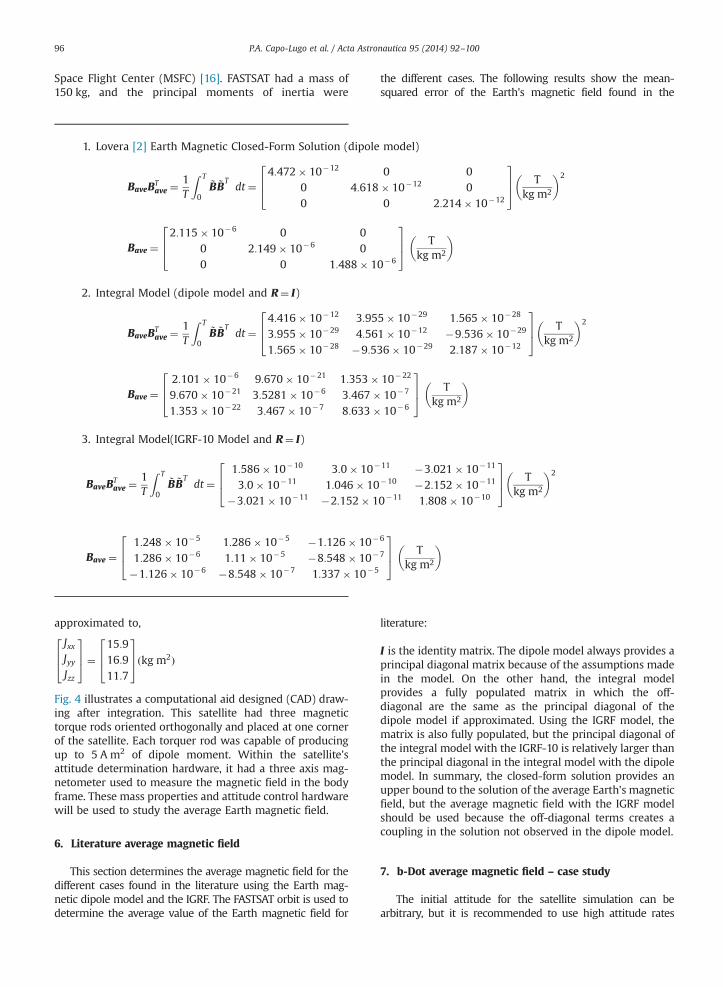
Space Flight Center (MSFC) [16]. FASTSAT had a mass of150 kg, and the principal moments of inertia were

1. Lovera [2] Earth Magnetic Closed-Form Solution (dipole model)

BaveBTave ¼

1T

Z T

0

~B ~BTdt ¼

4:472� 10�12 0 00 4:618� 10�12 00 0 2:214� 10�12

264

375 T

kg m2

� �2

Bave ¼2:115� 10�6 0 0

0 2:149� 10�6 00 0 1:488� 10�6

264

375 T

kg m2

� �

2. Integral Model (dipole model and R¼ I)

BaveBTave ¼

1T

Z T

0

~B ~BTdt ¼

4:416� 10�12 3:955� 10�29 1:565� 10�28

3:955� 10�29 4:561� 10�12 �9:536� 10�29

1:565� 10�28 �9:536� 10�29 2:187� 10�12

264

375 T

kg m2

� �2

Bave ¼2:101� 10�6 9:670� 10�21 1:353� 10�22

9:670� 10�21 3:5281� 10�6 3:467� 10�7

1:353� 10�22 3:467� 10�7 8:633� 10�6

264

375 T

kg m2

� �

3. Integral Model(IGRF-10 Model and R¼ I)

BaveBTave ¼

1T

Z T

0

~B ~BTdt ¼

1:586� 10�10 3:0� 10�11 �3:021� 10�11

3:0� 10�11 1:046� 10�10 �2:152� 10�11

�3:021� 10�11 �2:152� 10�11 1:808� 10�10

264

375 T

kg m2

� �2

Bave ¼1:248� 10�5 1:286� 10�5 �1:126� 10�6

1:286� 10�6 1:11� 10�5 �8:548� 10�7

�1:126� 10�6 �8:548� 10�7 1:337� 10�5

264

375 T

kg m2

� �

approximated to,

JxxJyyJzz

264

375¼

15:916:911:7

264

375ðkg m2Þ

Fig. 4 illustrates a computational aid designed (CAD) draw-ing after integration. This satellite had three magnetictorque rods oriented orthogonally and placed at one cornerof the satellite. Each torquer rod was capable of producingup to 5 A m2 of dipole moment. Within the satellite'sattitude determination hardware, it had a three axis mag-netometer used to measure the magnetic field in the bodyframe. These mass properties and attitude control hardwarewill be used to study the average Earth magnetic field.

6. Literature average magnetic field

This section determines the average magnetic field for thedifferent cases found in the literature using the Earth mag-netic dipole model and the IGRF. The FASTSAT orbit is used todetermine the average value of the Earth magnetic field for

the different cases. The following results show the mean-squared error of the Earth's magnetic field found in the

literature:

I is the identity matrix. The dipole model always provides aprincipal diagonal matrix because of the assumptions madein the model. On the other hand, the integral modelprovides a fully populated matrix in which the off-diagonal are the same as the principal diagonal of thedipole model if approximated. Using the IGRF model, thematrix is also fully populated, but the principal diagonal ofthe integral model with the IGRF-10 is relatively larger thanthe principal diagonal in the integral model with the dipolemodel. In summary, the closed-form solution provides anupper bound to the solution of the average Earth's magneticfield, but the average magnetic field with the IGRF modelshould be used because the off-diagonal terms creates acoupling in the solution not observed in the dipole model.

7. b-Dot average magnetic field – case study

The initial attitude for the satellite simulation can bearbitrary, but it is recommended to use high attitude rates

0.1 0.2 0.3 0.4 0.5 0.6 0.7 0.8 0.91

1.2

1.4

1.6

1.8

2

2.2

2.4

2.6

2.8

3

Orbits

ω (d

eg/s

ec)

Data PointsLine Fit

Fig. 6. Regression analysis for the damping coefficient (simulation).

0 0.5 1 1.5 2 2.5 3−4

−2

0

2

4

ωφ (

deg/

sec)

ωθ (

deg/

sec)

ωψ

(deg

/sec

)

0 0.5 1 1.5 2 2.5 3−1

0

1

2

3

0 0.5 1 1.5 2 2.5 3−2

−1

0

1

2

Orbits

Fig. 5. Angular velocity of a satellite using a b-dot controller.

P.A. Capo-Lugo et al. / Acta Astronautica 95 (2014) 92–100 97

to analyze the damping effects in the b-dot controller. For thiscase study, the attitude motion is setup so that the initialattitude angles are zero and the initial attitude rates are 31 s�1

in the pitch axis and 11 s�1 in the roll and yaw axes. Inaddition, KD ¼ 200;000 for the three axes of the satellite.Fig. 5 shows the simulated b-dot control solution for FASTSATfor this set of initial conditions. The top, middle, and bottomgraphs are, respectively, the roll, pitch, and yaw attitude ratesin the satellite's body frame. As shown in Fig. 5, the attituderates are damped in 2.5 orbits.

The average magnetic field, using the b-dot controller,can be obtained from any of the three curves shown inFig. 5. Using the pitch axis (middle graph) in Fig. 5, thepositive maximum point at the crest of every wave isselected. This value is plotted in Fig. 6 to determine the

exponential decaying function. The exponential function isdetermined by regression analysis. The ratio in Eq. (14a)describing the average magnetic field for Fig. 5 are equal to

Bave=J ¼ a=KD ¼ 6:897� 10�6 Tkg m2

� �ð15Þ

If the same analysis is performed for the other two axes, theresults are the same as in Eq. (15). Hence, Eq. (15) provides theaverage of the magnetic field per moment of inertia of thesatellite. The results in Eq. (15) show a very similar solution asin Section 6, but the Bave is a value larger than the solutionsshown in the literature (Lovera [2],Psiaki [1]). The differencebetween this new method and the mean square of themagnetic field is that this new method takes into considera-tion the rate damping effects of the magnetic torquers.

The following steps can be generalized to determinethe average magnetic field:

1.

Select a value for KD to determine kdot . 2. Use a high initial attitude rate for the three axes of the

satellite (51 s�1 is a good approximation).

3. Propagate the satellite orbit using the IGRF model and

the b-dot controller.

4. Extract the maximum or minimum points of the angle

rate data to determine the damping coefficient usingregression analysis.

5.

Use Eq. (14a) to determine the average Earth’s magneticfield per principal moment of inertia.

8. b-Dot average magnetic field validation

As mentioned before, FASTSAT was launched in 2010into a circular orbit at 650 km altitude. The b-dot controller

Fig. 8. Average magnetic field data point analysis (flight data).

0.5 1 1.5 2 2.5 3 3.5 4−2

−1

0

1

2

ωφ (

deg/

sec)

ωθ (

deg/

sec)

ωψ (d

eg/s

ec)

0.5 1 1.5 2 2.5 3 3.5 4

−3

−2

−1

0

0.5 1 1.5 2 2.5 3 3.5 4

−1

−0.5

0

0.5

OrbitsFig. 7. Tip-off rates using b-dot control (flight data).

P.A. Capo-Lugo et al. / Acta Astronautica 95 (2014) 92–10098

used the previous KD gain as the kdot gain for the b-dotcontroller. Fig. 7 shows the tip-off rates from the flight dataof the satellite after deployed from the rocket. In Fig. 7, themaximum tip-off rates are approximately 31 s�1 about thepitch axis and 11 s�1 about the roll and yaw axes. Inapproximately four orbits, the attitude rates are dampedwith the b-dot controller.

When kdot is specified as in Eq. (11), Fig. 5 shows thesimulation for the body attitude rates. Fig. 5 does not showa direct comparison to the rate damping shown in Fig. 7for FASTSAT. Although the time to do the rate damping isclosely related between the simulation (Fig. 5) and theflight data (Fig. 7), the relation shown in Eq. (11) is

validated to work in the simulation because kdot4ðR3Þ=ðμEÞ=I.

Finally, the average magnetic field per moment ofinertia shown in Eq. (14a) will be validated with the flightdata in Fig. 7. The three axes were analyzed to determinethe average magnetic field. This paper will show theresults for the roll axis because it shows a very nicedamping coefficient near 0.5 orbits. Fig. 8 shows themaximum values at each crest of the roll motion, and thedashed line is the regression line for the decaying expo-nential function. The damping coefficient, a, is equal to1:412. When ξ is substituted into Eq. (14a), the averagemagnetic field per moment of inertia equals to,

Bave=J ¼ 7:060� 10�6 Tkg m2

� �ð16Þ

Comparing Eq. (15) with Eq. (16), there is an error of 2:4%in the solution. This means that the method shown here todevelop the average magnetic field is validated against theflight data. In addition, the average magnetic fieldobtained through simulation provides a larger bound incomparison to the methods shown in the literature. Theaverage magnetic field in Eq. (15) is determined using thepitch axis, but, in Eq. (16), the same analysis is performedwith the flight data using the roll axis. The statement, that“the average magnetic field per moment of inertia is thesame in three axes of the satellite”, is also validated.

9. Conclusion

The average magnetic field of the Earth has beenstudied and developed with different methods and mod-els. All the methods shown in the literature [1,2,8] usedthe mean square error of the magnetic field to determine

P.A. Capo-Lugo et al. / Acta Astronautica 95 (2014) 92–100 99

the average magnetic field. All these mathematical modelsare dependent on the model of the Earth Magnetic Fieldwhich is very well known. In this paper, a simple andelegant method is proposed for estimating the averageEarth Magnetic Field. The b-dot approach is a very simplemethod that uses a derivative controller. It does notrequire complex mathematical model to determine theaverage magnetic field, and it only uses five simple steps tocalculate the average magnetic field per moment of inertiaof the vehicle.

Because this method uses the b-dot controller,the flight data can be downloaded in the first pass, andthe rates can be analyzed to update the flight computerwith a new average magnetic field. As shown in the paper,the simulated average magnetic field is closely related tothe value determine with the flight data (Eqs. (15) and(16)).

The main advantage of this method is that the averagemagnetic field per moment of inertia is the same in thethree axes of the satellite. This presents an advantage inthe solution of Euler's equation. If Euler's equation is usedfor a control scheme as is shown in the literature,

I _ω!þ ω!� I ω!¼ m!� b!

ECI

the control solution for the gains is always related to themean square error of the average magnetic field [1,2].Using this new method to determine the average magneticfield, the applied dipole moments can be related as theopposite of each other (meaning m3 ¼ �m2; m1 ¼�m3; and m2 ¼ �m1) so that Euler's equation can bewritten as

_ω!þI�1 ω!� I ω!¼ 2Bave

I

m2

m3

m1

264

375

This form of Euler's equation can be used to determine thecontrol gains or to develop a controller that does notrequire the use of the mean square error as shown in theliterature [1,2]. This form of Euler's equation will besubject of future work.

In conclusion, the process shown in this paper todetermine the average magnetic field can be very easilyimplemented and demonstrated with a b-dot controller.Also, the FASTSAT's flight data validates this new methodwhich provides interesting results for the development offuture attitude controllers based on the magnetic field. Asshown in the solution, this method based on the b-dotcontroller reduces the mathematical complexity shown inthe literature.

Appendix A. Proof of Eqs. (10) and (12)

The transfer function for a closed-loop system with aunit feedback is described as

ωðsÞωr sð Þ

¼ G sð Þ1þG sð Þ

From Fig. 3(b),

G sð Þ ¼ KDBave

Js

Solving the closed-loop equation for the given GðsÞ, thetransfer function is defined as,

ωðsÞωrðsÞ

¼ KDBave=JsþðKDBave=JÞ

¼ ξ

sþξ

so that,

ξ¼ KDBave

J

Performing the inverse Laplace transform of the previoustransfer function equation, the differential equationobtained is

_ωðtÞþξωðtÞ ¼ ξωrðtÞ ðA:1ÞFor this equation, the time is scaled down by using thefollowing relation:

τ¼ t=T ðA:2ÞThe Scaling theorem of the Laplace transform says that,

ℒ f ðatÞ� �¼ 1aF

sa

� �ðA:3Þ

a is an arbitrary constant larger than zero. The followingrelations can be obtained from each term in Eq. (A.1) usingEq. (A.3),

ℒ _ωtT

� � ¼ T2sωðTsÞ ðA:4aÞ

ℒ ξωtT

� � ¼ TξωðTsÞ ðA:4bÞ

ℒ ξωrtT

� � ¼ TξωrðTsÞ ðA:4cÞ

Using Eq. (A.4), the Laplace transform of Eq. (A.1) is,

ωðsTÞωrðsTÞ

¼ ξ=Tsþξ=T

ðA:5Þ

Eq. (A.5) is Eq. (10). Using the Scaling theorem once again,the following Laplace transform can be obtained,

ℒ e�ðat=TÞutT

� � ¼ 1

sþ aT

ðA:6Þ

where uðt=TÞ is the unit step function. With Eq. (A.6), theinverse Laplace transform of Eq. (A.5) equals to,

ωtT

� �¼ ξ

Te�ðξ=TÞtωr

Using the relation in Eq. (A.2), Eq. (12) is obtained asshown in the following equation.

ω τð Þ ¼ ξ

Te� ξτωr ðA:7Þ

References

[1] Mark L. Psiaki, Magnetic Torquer Attitude Control via AsymptoticPeriodic Linear Quadratic Regulation, J. Guid. Control Dyn 24 (2)(2001) 386–394.

[2] M. Lovera, A. Astolfi, Global magnetic attitude control of spacecraftin the presence of gravity gradient, IEEE Trans. Aerosp. Electron.Syst. 42 (3) (2006) 796–806.

P.A. Capo-Lugo et al. / Acta Astronautica 95 (2014) 92–100100

[3] Pedro A. Capo-Lugo, Peter M. Bainum, Orbital Mechanics andFormation Flying, a Digital Control Perspective, Woodhead Publish-ing, Cambridge, UK, 2011.

[4] Manoj Nair, Retrieved from International Geomagnetic Reference Field:⟨http://www.ngdc.noaa.gov/IAGA/vmod.igrf.html⟩, January, 2010.

[5] James R. Wertz, Attitude Determination and Control, Reidel Publish-ing Company, Dordecht, Holland, 2002.

[6] S. Maus, et al., The 10th Generation International GeomagneticReference Field, Phys. Earth Planet. Inter. 151 (2005) 320–322.

[7] Jan Tommy Gravdahl, Magnetic attitude control for satellites, in:Proceedings of the 43rd IEEE Conference on Decision and Control,Atlantis, Paradise Island, Bahamas, December 14–17, 2004.

[8] Rafa Wisniewski, Linear Time Varying Approach to Satellite AttitudeControl Using Only Electromagnetic Actuation (1997).

[9] James R. Wertz, Wiley J. Larson, Space Mission Analysis and Design,3rd ed. Microcosm Press and Kluwer Academic Publishers, Califor-nia, USA, 1999.

[10] M. Reyhanoglu, J.R. Hervas, Three-axis magnetic attitude control algo-rithms for small satellites, in: Proceedings of the 5th International

Conference on Recent Advances in Space Technologies (RAST), Istanbul,Turkey, 2011, pp. 897–902.

[11] Norman S. Nise, Control System Engineering, 4th ed. John Wiley &Sons, USA, 2004.

[12] Katsuhiko Ogata, System Dynamics, 4th ed. Prentice Hall, New Jersey,USA, 2004.

[13] Ron Larson, Betsy Farber, Elementary Statistics, Picturing the World,5th ed. Prentice Hall, Boston, USA, 2012.

[14] F. Marter, P.K. Pal, M. Psiaki, Active magnetic control system forgravity gradient stabilized spacecraft, in: Proceedings of the 2ndAnnual AIAA/USU Conference on Small Satellites, Utah State Uni-versity, Logan, Utah, 1988.

[15] William H. Steyn, Comparison of low-Earth-orbit satellite attitudecontroller submitted to controllability constraints, J. Guid. ControlDyn. 17 (4) (1994) 795–804.

[16] Brandon DeKock, Devon Sanders, Tannen VanZwieten, Pedro Capo-Lugo,Design and integration of an all-magnetic attitude control system forFASTSAT-HSV01 multiple pointing objectives, in: Proceedings of the 34thAnnual Guidance, Navigation, and Control Conference, Breckenridge,Colorado, February 4–9, 2011.