Page 1
HAL Id: hal-01162071https://hal.archives-ouvertes.fr/hal-01162071
Submitted on 9 Jun 2015
HAL is a multi-disciplinary open accessarchive for the deposit and dissemination of sci-entific research documents, whether they are pub-lished or not. The documents may come fromteaching and research institutions in France orabroad, or from public or private research centers.
L’archive ouverte pluridisciplinaire HAL, estdestinée au dépôt et à la diffusion de documentsscientifiques de niveau recherche, publiés ou non,émanant des établissements d’enseignement et derecherche français ou étrangers, des laboratoirespublics ou privés.
The Bank Capital Regulation (BCR) ModelHyejin Cho
To cite this version:
Hyejin Cho. The Bank Capital Regulation (BCR) Model. 2015. �hal-01162071�
Page 2
Documents de Travail du Centre d’Economie de la Sorbonne
The Bank Capital Regulation (BCR) Model
Hyejin CHO
2015.21
Maison des Sciences Économiques, 106-112 boulevard de L'Hôpital, 75647 Paris Cedex 13 http://centredeconomiesorbonne.univ-paris1.fr/
ISSN : 1955-611X
Page 3
The Bank Capital Regulation (BCR) Model
Hye-jin Cho†
†Department of Economics, University of Paris 1, Pantheon-Sorbonne, PARIS, FRANCE
Abstract. The motivation of this article is to induce the bank capital management
solution for banks and regulation bodies on commercial banks. The goal of the paper
is intended to mitigate the risk of a banking area and also provide the right incentive
for banks to support the real economy.
Keyword: Demand Deposit, On-balance-sheet risks and off-balance-sheet risks,
Portfolio composition, Minimum equity capital regulation.1
JEL Classifications: C62; C63 ; D01 ; G10 ; G21
Part I Introduction
In Europe, after the Basel 1 (1988) accord, the banking supervision Accords in
Basel, Switzerland, Basel 2 (1999) and Basel 3 (2010) have been evolved. The issuer,
the Basel Committee on Banking Supervision (BCBS), advised about credit risk
(1988.07) at the Basel 1 and amended about market risk (1996.01) with the Basel 1
Amendment. In the revised framework of the Basel 2, operational risk (2004.06) was
introduced and enhanced at the Basel 3 (2010.12). In this overall perspective, these
Basel Capital Rules have been enhanced up to the Basel 3. For example, the scope of
operational risk is enlarged. This requires some reasonable motivation since banks face
the situation to manage the cost to follow banking capital regulation rules. Of particular
significance is that the government needs to regulate banks to prevent panic from the
systemic banking crisis.
Much interest has been aroused in cascading failure of bank run prevention. For
example, Friedman and Schwartz (1963) observe large costs imposed on the economy of
United States caused by bank runs in the 1930s. Upon on much more recent data, in
systemically important banking crises of the world from 1970 to 2007, the average net
1 This work was achieved through the Laboratory of Excellence on Financial Regulation (Labex ReFi) supported
by PRES heSam under the reference ANR-10-LABX-0095. It benefitted from a French government support
managed by the National Research Agency (ANR) within the project Investissements d'Avenir Paris Nouveaux
Mondes (invesments for the future Paris-New Worlds) under the reference ANR-11-IDEX-0006-02. My special
thanks go to my supervisor Raphael Douady, my co-supervisor Duc Khuong Nguyen and Jean-Bernard
Chatelain for a good comment in 8th
Doctorissimes in the University of Paris1. Invaluable inspiration to figure
out financial economic methodology on this article was furnished by Chris Shannon, Frank Riedel, Nobuhiro
Kiyotaki and all participants at seminars in 2014 by the university of Paris1 (Panthéon Sorbonne), the 2014
International Conference on Economic and Financial Risks by the University of Poitier, Advanced in Stochastic
Calculus by University of Bielefeld 2014, the 14th
SAET conference by the Waseda university, the 14 FRAP
conference by Oriel College, Oxford University and 2014 Extreme Events in France by the ESSEC. I wish also
to record my affection to my family and JP.
Documents de travail du Centre d'Economie de la Sorbonne - 2015.21
Page 4
recapitalization cost to the government was 6% of GDP (Gross Domestic product).
Fiscal costs associated with crisis management were averaged 13% for GDP (16% of GDP
if expense recoveries are ignored), and economic output losses were averaged about 20%
of GDP during the first four years of the crisis. Otherwise, if the government decides to
adopt the Basel capital regulation framework, the adoption cost will influence the
economy of countries. Either households or banks, related parties to economy should pay
for the Basel capital regulation as the preventive method in the banking business cycle.
An OECD (The Organization for Economic Cooperation and Development) study
released on 17 February 2011, estimated that the medium-term impact of the Basel III
implementation on GDP growth would be in the range of 0.05% to 0.15% per year.
Economic output would be mainly affected by increase in banks’ lending spreads, as
banks pass a rise in bank funding costs, due to higher capital requirements, to their
customers. Therefore, the situation is that banks are struggling to manage the regulation
cost and the government wants to defend about nationwide contagion of other banks.
Part II The macro-prudential approach to financial regulation covering on-
balance-sheet and off-balance-sheet (OBS)
Insofar as systemic risk is concerned, risks that firms, households and reserve
banks and commercial banks face are highly linked to each other. Seen from this point
of view, the banking industry and the monetary policy have particular relevance to
systemic risk. Undoubtedly, it goes without saying that financial contagion problems
through international banks should be measured in the manner of systemic risk
management. With the macro-prudential approach, it is highly probable that systemic
risk is explained by the static model of the general equilibrium. Because on-balance-
sheet and off-balance-sheet (OBS) risks are structurally segmented annually or
periodically by financial statements containing the balance sheet. Even though domino
effects or contagions can be understood as movements having the future tendency to
figure out solutions toward the future, scope of regulation should be articulated by
categorization of on-balance-sheet and off-balance-sheet (OBS) risks in the static model.
Thus the macro-prudential approach to financial regulation covering on-balance-sheet
and off-balance-sheet (OBS) risks is intimately linked with the general equilibrium (GE)
approach.
On-balance-sheet risks are presented in a fourfold manner and are divided into
credit risk, market risk, liquidity risk and systemic risk. Assets of banks have credit risk
and market risk. Credit risk is the risk that a borrower will default on any type of debt
by failing to make required payments. Market risk is the risk of losses in positions
arising from movements in market prices. In case of liquidity risk, there are two major
situations. One is emergency capacity of banks. When an illiquidity event takes place,
an affected bank typically must borrow funds at interest rates exceeding those paid by
other institutions. Another is about the stability of the banking system in case of
inducing a large number of depositors to seek withdrawals. I would say liquidity risk in
regard of demand deposit is on-the-balance-sheet risks of banks. Credit, market and
liquidity risk are portrayed in considerable individual details but systemic risk is negative
externality or adverse spillover effect stemming from transaction in which they were not
participants. Distinguished from credit risk containing sovereign risk (government risk),
counterparty risk (unincorporated entities’ risk exposed to financial risk, usually
Documents de travail du Centre d'Economie de la Sorbonne - 2015.21
Page 5
referring to governments, national banks), systemic risk is the risk of collapse of an
entire financial system or the entire market, as opposed to risk associated with any
individual entity, group or component of a system. George G. Kaufman and Kenneth
E. Scott (2003) define “systemic risk” in imprecise terms as below:
”Systemic risk refers to the risk or probability of breakdowns in an entire system,
as opposed to breakdowns in individual parts or components, and is evidenced by co-
movements (correlations) among most or all the parts.”
Darryll Hendricks (2009), who is a practitioner, suggests a more theoretical
definition from sciences in which the term originated:
“A systemic risk is the risk of a phase transition from one equilibrium to
another, much less optimal equilibrium, characterized by multiple self-reinforcing
feedback mechanisms making it difficult to reverse.”
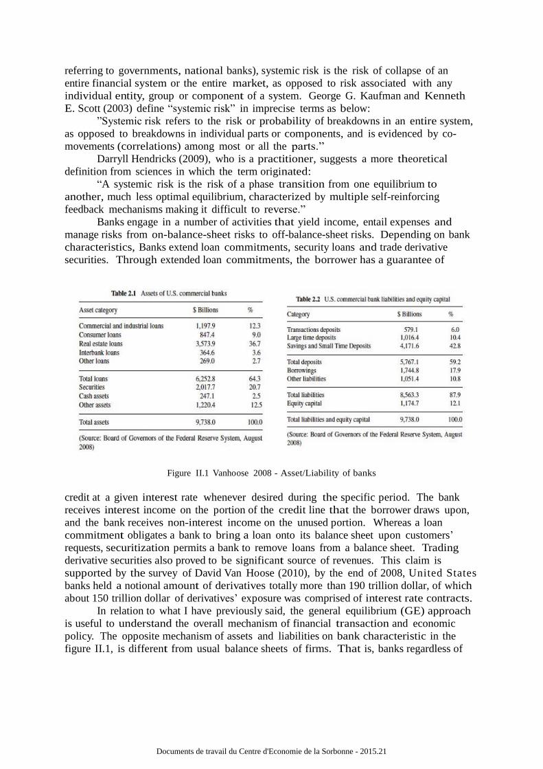
Banks engage in a number of activities that yield income, entail expenses and
manage risks from on-balance-sheet risks to off-balance-sheet risks. Depending on bank
characteristics, Banks extend loan commitments, security loans and trade derivative
securities. Through extended loan commitments, the borrower has a guarantee of
Figure II.1 Vanhoose 2008 - Asset/Liability of banks
credit at a given interest rate whenever desired during the specific period. The bank
receives interest income on the portion of the credit line that the borrower draws upon,
and the bank receives non-interest income on the unused portion. Whereas a loan
commitment obligates a bank to bring a loan onto its balance sheet upon customers’
requests, securitization permits a bank to remove loans from a balance sheet. Trading
derivative securities also proved to be significant source of revenues. This claim is
supported by the survey of David Van Hoose (2010), by the end of 2008, United States
banks held a notional amount of derivatives totally more than 190 trillion dollar, of which
about 150 trillion dollar of derivatives’ exposure was comprised of interest rate contracts.
In relation to what I have previously said, the general equilibrium (GE) approach
is useful to understand the overall mechanism of financial transaction and economic
policy. The opposite mechanism of assets and liabilities on bank characteristic in the
figure II.1, is different from usual balance sheets of firms. That is, banks regardless of
Documents de travail du Centre d'Economie de la Sorbonne - 2015.21
Page 6
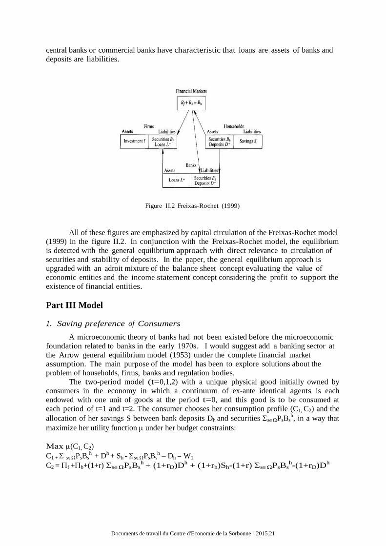
central banks or commercial banks have characteristic that loans are assets of banks and
deposits are liabilities.
Figure II.2 Freixas-Rochet (1999)
All of these figures are emphasized by capital circulation of the Freixas-Rochet model
(1999) in the figure II.2. In conjunction with the Freixas-Rochet model, the equilibrium
is detected with the general equilibrium approach with direct relevance to circulation of
securities and stability of deposits. In the paper, the general equilibrium approach is
upgraded with an adroit mixture of the balance sheet concept evaluating the value of
economic entities and the income statement concept considering the profit to support the
existence of financial entities.
Part III Model
1. Saving preference of Consumers
A microeconomic theory of banks had not been existed before the microeconomic
foundation related to banks in the early 1970s. I would suggest add a banking sector at
the Arrow general equilibrium model (1953) under the complete financial market
assumption. The main purpose of the model has been to explore solutions about the
problem of households, firms, banks and regulation bodies.
The two-period model (t=0,1,2) with a unique physical good initially owned by
consumers in the economy in which a continuum of ex-ante identical agents is each
endowed with one unit of goods at the period t=0, and this good is to be consumed at
each period of t=1 and t=2. The consumer chooses her consumption profile (C1, C2) and the
allocation of her savings S between bank deposits Dh and securities sPsBsh, in a way that
maximize her utility function under her budget constraints:
Max (C1, C2)
C1 + sPsBsh
+ Dh + Sh - sPsBs
h – Dh = W1
C2 = f +b+(1+r) sPsBsh
+ (1+rD)Dh + (1+rh)Sh-(1+r) sPsBs
h-(1+rD)D
h
Documents de travail du Centre d'Economie de la Sorbonne - 2015.21
Page 7
Where W1 for her initial endowment of the consumption good, f +b for respectively
profits of the firm and of the bank (distributed to the consumer-stockholder at t=2).
Bh denotes for securities, D
h for bank deposits. S h denotes for savings. r, rD , rh are
interest rates paid by securities, deposits and savings. For each future state of the world
s (s) one can determine the price P s the contingent claim that pays one unit of
accounts in state s and nothing otherwise.
The consumer has a well-defined set of desires (”preference”), which can be
represented by a numerical utility function. In addition, we assume that the consumer
chooses optimally, in the sense that they choose the option with the highest utility of
those available to them. It implies that a consumer is solving an optimization problem.
An optimization problem has three key components.
a. Selected object The consumer chooses her consumption profile (C1 , C2 ) and
allocation of her savings Sh between bank deposits Dh and securities Bh. If real assets Sh -
sPsBsh – Dh is non-negative, it implies real assets are sufficient to support the
household economy.
b. The objective function The consumer maximizes her utility function . is assumed
to be increasing and concave. Notice that preferences are contingent states and do not
fit the standard Von Neumann-Morgenstern representation. Incompleteness of
preference becomes apparent that decision makers cannot make a decision in the
ambiguous situation. However, even though one individual or one factor doesn’t decide,
the regulator decides the policy with a foretaste of what is to come after annual closing
accounts.
c. Constraints
Cash-in-advance 0D h W1, The paper will be based on the Cash-in-advance
constraint. This approach that was introduced by Clower (1967) is the requirement
that each consumer or firm must have sufficient available cash before they can buy
goods.
Price of security h under Uncertainty sPsBsh
(resp. sPsBsf, sPsBs
b) implies the
price of securities by the absence of arbitrage opportunities. A bank issues (or buys) a
security h (intepreted as a deposit or a loan) characterized by the array Bsh
(s) (resp. Bsf,
Bsb) of each payoff in all future states of world
Interior Solution The consumer’s program (Ph) has an interior solution only when
interest rates are equal: r = r D
Preference of Savings In the Arrow-Debreu model, money is redundant in the
market. Households are indifferent about the composition of savings. In the paper, the
household has preference to increase the budget to collect savings Sh and affected by risk
levels of securities, deposits and real assets. Savings Sh is the sum of Securities sPsBsh
, Deposits Dh and Real Assets Sh-( sPsBsh
+Dh).
Documents de travail du Centre d'Economie de la Sorbonne - 2015.21
Page 8
d. Arguments
There are concerns about savings that are substituted into consumption by the
household like Covas-Fujuta (2010). Diaz (2005) adds no capital requirement at basics
to reduce consumption and increase savings by the household. Haslag (2001) assumed
that return to money is positively related to the money growth rate that is a random
variable, gross real returns to savings are random. His realized gross real return to
savings indicates that the gross real return to savings is a weighted sum of capital and
fiat money (which derives its value from government regulation or law, so called as ’fiat
currency’). The weight is the share of agent’s asset.
In the Waller model (2004), Savings are very passively selected by the household
depending upon decisions at the previous period. Middle-aged agents have already
earned their wage income, as the wage during period t was determined by the previous
period’s interest rates (a level of the capital stock). Also, they have already decided how
much to consume and save (since savings are a fixed fraction of wage income), but they
have not yet decided how to allocate their savings between capital and fiat currency.
What these middle aged agents want at this point is just the highest possible interest rate
between period t and t + 1, so that they can obtain the best possible return on their
savings and can thus consume as much as possible during their period of old age. In the
third period of life, retired agents consume their savings and exit the model.
Practically, Christensen-Meh-Moran (2011, Bank of Canada) mentioned, at the
timing of events, households deposit savings at banks that use these funds as well as their
own net worth to finance the entrepreneur’s projects. In the investment frame, exiting
(failing to return from the project) agents sell their capital for consumption goods and
surviving agents buy this capital as part of their consumption-savings decision.
However, in reality, even though the agent has a house, they need to spend
expenditure for renting, maintenance and extension of houses. Savings and real asset
portion are large enough to make the loan from banks. It is hard to explain price
fluctuation of houses and savings on the economy by depending upon the interest rate
of capital stock and deposit, or perfect substitution of consumption. For households, the
preference of savings is the matter about existence of household economy making future
benefits and directly affecting to the welfare of any individual.
House-price appreciation by the model of Goodhart-Kashrap-Tsomocos (2012) is
impressive. Reducing deposit defaults induces more savings circulated by the bank and
less self-insurance and by the end, the reduction in self-insurance reduces the number of
houses for sale in a good state, which means that house-price appreciation in the boom
is higher than otherwise. Most of all, the market incompleteness with deadweight costs
of default distorts the housing market. Wealthy agents endowed with houses make their
saving decisions accounting for the possibility that deposits will not be fully repaid.
When default penalties for banks are low, then households internalize risks putting less
wealth into the banking system and hold more in the form of houses. This choice
increases the supply of houses that is available in boom, which lowers house prices and
raise welfare for agents entering the housing market at that time. To insure that house
price reduction in the bad state of the world, households P and F are also presumed to
have lower wealth. Likewise, the non-bank is endowed with lower capital in period 1 as
well as in the bad state of the world. This model describes the house bubble
phenomenon interestingly.
Documents de travail du Centre d'Economie de la Sorbonne - 2015.21
Page 9
In the model of Lucas (1995), to support the incompleteness of markets, he
pointed out savings that the young split their savings between bank deposits, which
promise a fixed nominal return, and a bank equity, which yields an uncertain real
dividend. In addition, because a constant fraction of initial wealth is saved, there is no
distortion due to fixed nominal interest payments on deposits. Hence regardless of
deposits, the bank equity is related to the real effect of monetary policy.
In the paper, at the framework of securities, deposits and real assets with savings,
firstly, the relation between savings and real assets (especially houses) can be much more
attached. Secondly, deposits included in the total saving amount which are escaped
from the one-sided thinking that deposits are equal to savings and can be perfectly
substituted to consumption. Thirdly, Securities at uncertainty are affecting to the
investment portfolio of households. These dynamics are explained by the following
academical detail.
Households choose (C1 , C2 , S1 , S2 , R1) taking prices (W1 , W2 ) as given.
Formally, if we consider the 4-factor model containing banks, because banks have the
special financial structure having deposits as liabilities and loans as assets, we need to
have the different mindset from generally accepted accounting principles about debit and
credit accounts. The general equilibrium (GE) diagram is similar with the balance sheet.
Distinguishably, the money flow in the paper starts at the bank transaction which is
“deposits and borrowings” as liabilities and “claims to corporate” as assets.
Then, deposits of household are the amount to be accumulated in banks.
Conveniently, riskier investments than deposits for household are categorized as
securities.
Savings are moving in the real household economy by capital circulation of
securities, deposits and real assets. In addition, the welfare of each household is moving
from dynamics of accumulated savings. In the overlapping generation model, wealth is
always given and manages the household economy easily by each generation. In reality,
one who didn’t get a house as a legacy, she should spend quite a long time to have a
house or rent a house. Attention about fundamental wealth related to non-working
capital of a household economy should be emphasized. If the consumer spends his
income entirely, the total amount W1 may be spent totally and can be bounded. In this
manner, the household always has their fundamental welfare to manage the household
economy and consumption can be naturally deduced from the framework of household
economy. That is, W1 is the budget constraint and the market information is
incomplete so we cannot deduce the real variable of consumption in reality. W1 and
incompleted market information are not enough to deduce the real variable of
consumption. In terms of the working capital, we are not so surprised to know that
capital has various liquidities. For example, a household wants to spend money on a daily
basis but should reduce the amount of money by spending it to have fundamental living
basis like houses. In the paper, the financial budget constraint is bounded within the W1
except for S1 because S1 is the summation of securities, deposits and real assets. These
are vital factors to operate household economy related to financial markets. The working
capital concept at the household economy is evoked within the general equilibrium in the
paper. In the perspective that the industrial characteristics of banks mainly operated by
capital, it makes sense to us that consideration about the household economy should be
balanced with the working capital concept of banks.
Documents de travail du Centre d'Economie de la Sorbonne - 2015.21
Page 10
Then, why we need to define return R1 in this model? Simply, we think of three
variables of W for endowment, S for savings and C for consumption. We assume that
the concept of the golden-rule saving rate in Chapter 1 of Barro and Sala-i-Martin, n
denotes for the constant exogenous population growth rate, and d is for the constant
exogenous rate of depreciation of capital. We know the house saving rate is 5% (usually
2-11%, OECD, Economic Outlook n.91, June 2012). The amount of savings in the
economy should grow as population grows. To support this insured saving amount
caused by population growth, the return should be enough to make profits to cover the
insurance expense in the economy with the general equilibrium (GE) perspective. Then,
we can assume the worst scenario like a bank-run case. Even though the fix amount of
saving deposits is secured, the loss amount induced from total savings by the end -
insured savings will go to the consumption part. In this overall perspective of an
equilibrium, insuring savings of households seems plausible to support the economy of
households, yet it requires further understanding about the profitable dynamic
mechanism to operate the economic cycle. I would say the original form is mainly
based on the BCR general equilibrium model diagram presenting as the balance-sheet
format as it can be because on-balance-sheet factors are reflected by two regards - the
money flow perspective (profit) and the economic status perspective (net present
value).
Original form (savings containing real assets)
Max (C1, C2)
C1 + sPsBsh
+ Dh + Sh - sPsBs
h – Dh = W1
C2 = f +b+(1+r) sPsBsh
+ (1+rD)Dh + (1+rh)Sh-(1+r) sPsBs
h-(1+rD)D
h
Simplified form for calculation (savings containing real assets)
Max (C1, C2)
C1=W1-S1
C2=R1+W2-(1+r)S1-S2
We have the first order condition of consumption at period 1 and 2 as below. 𝐿
C1 = ’(C1, C2) - = 0
𝐿
C2 = ’(C1, C2) - = 0
We know the Lagrange multiplier is 0 as = 0, by the 𝐿
S1, the first order condition
of savings at period 1 and by the 𝐿
𝑅1, the first order condition of return from initial
investment. In addition, we get (1+r1) = 0 by the 𝐿
S1, the first order conditon of savings
at period 1.
Therefore, what is get from checking the first order condition of household
problem is that households consume today or tomorrow regardless of a banking money
flow and it is not affected by the return of initial savings. ’(C1, C2) = 0 denotes as time
indifference about consumption preference. Households operate the household economy
related to banks regardless of consumption for today or tomorrow. We conclude
Documents de travail du Centre d'Economie de la Sorbonne - 2015.21
Page 11
consumption choice is not affected by return of initial savings r1 at the frame of
banking money flow related to household.
The house expense portion in deposits held with MFIs (Monetary Financial
Institutions) is the asset that can induce the future benefit and considered as priority to
invest for a long time. For example, among loans to households of MFIs (5231 billion
euros), loans for house purchase are 74%, 3858.1 billion euros in 2013. Note that we
focus on the money transaction started from the bank balance sheet, in the concept of
savings, House fee is deduced from Sh-sPsBsh-Dh Where h is the period of household.
If we suppose the house fee is not contained in savings as below.
Simplified form for calculation (savings without real assets)
Max (C1, C2) = 0
C1 + 1P1B1h
+ D1 = W1
R1+C2+(1+r) 1P1B1h
+ (1+r1)D1-(1+r) -2P2B2
h-D2=W2
Also, C1 = (W1 –S1)+(S1- 1P1B1h
+ D1
The first-order condition 𝐿
C1 = ’(C1, C2) - = 0
𝐿
C2 = ’(C1, C2)- = 0
𝐿
D1 = 0
𝐿
D1 - (1+r1) = 0
𝐿
D2 = 0 ’(C1, C2)=0
𝐿
1P1B1h - (1+r1) = 0
𝐿
1P1B1h = 0
𝐿
r1 = ( 1P1B1
h + D1) = 0
In conclusion, ’(C1, C2)=0 (time indifference about consumption preference) is
the same condition regardless of real assets whether it is contained in savings or not.
Consumption choice is not affected by the interest rate r1 for initial savings
(same condition regardless of real assets whether is contained in savings or not) and
summation of securities and deposits 1P1B1h+D1. Evidently, this condition
appears in this banking model when we ignore real assets which is most stable in the
household economy and can be interpreted as the big portion expense and the
intangible asset producing future benefits. Therefore, with the condition that real assets
are contained in savings, we can explain the house economy affected by the proportion
of securities and deposits.
First intention to choose the general equilibrium model in the paper is to offer
understandable method to the academic field and professional field. In the practice, the
reserve bank has many methods and even they want more methods together in the
weighted way. As I can do, I am intending to use real variables than random variables and
a lot of Lagrange methods which is very general way to use the general equilibrium. The
saving composition matter is more specifically supported by the following empirical
data.
Documents de travail du Centre d'Economie de la Sorbonne - 2015.21
Page 12
The deposit amount traded is different depending upon factor composition of
economic models. For example, the European Central Bank announces the Euro areas’
deposit amounts for the 4th quarter in 2013 in the Euro areas. Gross saving amount of
households is 2521.3 billion euros (growth rate: 2.4). Deposits by non-financial
corporations are 1870.7 billion euros. (growth rate: 6.7). Deposits by Insurance
corporations and pension funds (financial intermediaries) are 653.2 billion euros.
(growth rate: -5.3). Deposits by other financial intermediaries are 1854.1 billion euros
(growth rate -3.1). Deposits by government are 440.8 billion euros (growth rate: -1.8).
Deposits by non-euro area residents are 2522.9 billion euros (growth rate: -11.2).
Therefore, without consideration about deposits by non-financial corporations (1870.7),
the comparison between deposits by household (2521.3) and deposits by financial
intermediaries (653.2+1854.1=2507.3) is naive explanation.
Loans for house purchase is 3858.1 billion euros. (growth rate: 0.7). It is Long-
term liability affecting the existence of household economy. In addition, the total
(7341.7) of deposits by insurance corporations, pension funds (653.2, -5.3), other
financial intermediaries (1854.1, -3.1), non-financial corporations (1870.7), government
(440.8), non-euro area residents (2522.9) are. Also, total (7752.2) of deposits by
household (2521.3, 2.4) and Loans for house purchase (3858.1, 0.7) and other loans
(796.7, -1.6), consumer credit (576.1, -3.0) are.
Loans for house purchase
(3858.1, 0.7)
other loans (796.7, -1.6)
consumer credit (576.1, -3.0)
total 7341.7
(billion euros, growth rate)
insurance corporations and pension funds
(653.2, -5.3)
other financial intermediaries (1854.1, -3.1)
non-financial corporations are (1870.7, 6.7)
government (440.8, -1.8)
non-euro area residents (2522.9, -11.2)
total 7752.2
Empirical balance when the capital of a household economy is concerned
Ref: European Central Bank, the 4th quarter in 2013
Savings Sh are the sum of Securities sPsBsh, Deposits Dh, Real assets Sh -
sPsBsh – Dh. Households try to control the balance of assets and liabilities because in
the situation of uncertainty, to maintain enough Deposits Dh for the economic existence
of households, households need to invest on securities as of sPsBsh posed on
uncertainty conditions. Mainly, real assets imply the budget for houses which can afford
to manage the residence and invested real assets. For example, if the household has an
apartment and there is the redundancy after spending the investment on securities and
deposits, it can be the maintenance fee for house decoration or big furniture purchases.
The importance of portion for houses is considerable. Otherwise, if real assets are
negative, hence, savings of households are less than the amount of securities and deposits.
Even though, the amount of operation in the household is enough with securities and
deposits. In the conservatism on the house budget, we can consider the effect on
housing. In the paper, Houses of households is considered as future economic assets that
support each member of households to make productions.
Through the general equilibrium approach, the link from the bank problem to the
household problem is naturally connected. Also, the following technical finding by usage
of same accounts at the household problem induces direction of regulation on banks like
Documents de travail du Centre d'Economie de la Sorbonne - 2015.21
Page 13
the portfolio analysis and initial GDP consideration. The following are technical findings
with saving preference.
Suppose that s G, B, G=Good, B=Bad. In the case 1, risk aversion is a s
below. (resp. risk-taking case)
= G, B, C1+sPs=BBs=Bh+D
h+Sh-sPs=GBs=G
h-D
h=W1
In this case, portfolio analysis should be detected by regulation because the
situation can be changed depending on the status.
In the case 2, incompleteness preference can be considered.
= G, B, no choice, no choice can be selected by the choquet expectation CE((x)) =
mincore() E((x)) where core() = S : (A) (A) for all AS
C1+0+Dh+Sh-0-D
h=W1 and D
h offset, hence C1+
𝐶2
1+𝑟ℎ=W
Initial GDP is caused by partition of initial endowment that is combination of
consumption set. Hence, regulation direction is originated from initial GDP in this case.
2. Borrowing composition of Firms - Additional session is in the Part IV.6
The firm chooses its investment level I and its financing (through Real
Assets sPsBsh
+ Dh, Liabilities to banks sPsBsh
+ Dh -Lfr (Or Liabilities to
central banks Lfr) in a way that maximizes its profit:
Max f (P f)
f =(I)+rf (sPsBsh+ Dh)-rL
bank(Dh+
sPsBs
h-Lfr)-rL
frLfr
I=Sh=Dh+sPsBsh
Where denotes the production function of the representative firm. r is the premium
of firm’s real assets. rLbank
, rLfr are interest rates on bank loans and federal reserve
bank loan. Dh denotes for bank deposits. Bh denotes for securities. Especially Bfr denotes
for securities of federal reserve banks. Lfr are loans claimed by the firm to the federal
reserve bank. For each future state of the world s (s), one can determine the price Ps
of the contingent claim that pays one unit of accounts in a state s and nothing otherwise.
I is the investment level and S h denotes for savings.
Interior Solution P has an interior solution only when: r= rLbank
=rLfr
The Modigliani-Miller (MM) theorem projects a theme of a theorem on capital
structure. The basic theorem states that, under a certain market price process (the
classical random work) and an efficient market, in the absence of taxes, bankruptcy
costs, agency costs and asymmetric information, the value of a firm is unaffected by how
that firm is financed. Firms are indifferent about the composition of borrowings. Given
the proposition II of the Modigliani-Miller (MM) theorem, a higher debt-to-equity ratio
Documents de travail du Centre d'Economie de la Sorbonne - 2015.21
Page 14
leads to a higher required return on equity because of the higher risk involved for
equity-holders in a company with debt. rE=r0+𝐷
𝐸 (r0-rD) where rE is the required rate of
return on equity or cost of equity, r0 is the company unlevered cost of capital (ie. Assume
no leverage, rD is the required rate of return on borrowings or cost of debt and 𝐷
𝐸 is the
debt-to-equity ratio under two assumptions: (1) no transaction costs exist. (2) individuals
and corporations borrow at the same rates. However, on the surface, given same ratios of 𝐷
𝐸, two different sized banks are distortly intepreted. Even though this proposition is
induced in the absence of the bankruptcy costs, merges of banks like “too big to fail”, so
called “the size game among big banks, are considerable. Thus it is certainly worth
inquiring D+E behind it’s apparent dynamics of 𝐷
𝐸.
The BCR model provides a key with which to unlock riddles of firms’ borrowing
compositions. The borrowing composition of firms imparted dynamics with the
preference to maintain Real Assets sPsBsh
+ Dh. Regardless of equilibrium, firms
prefer to loan from central banks (so called as bonds) than commercial banks. Among the
Dh and sPsBsh, Firms prefer to have Dh because of financial stability and preference
about certainty. The model reflects the tendency of banks toward the big size with Real
Assets. In the economic existence respect of banks, banks have responsibility to operate
the dynamics of the debt-to-equity ratio 𝐷
𝐸 and maintain the economic entity of Real Assets
D+E in the economy of countries.
Given the firm’s problem, we have ambiguity about change of firms because of
investments or loan status. Precise explanation about the relation with commercial banks
and central banks should be offered. In the general equilibrium (GE), firms choose labor
cost and manage the capital for production or business process but labor effect is hard to
be clarified with certain connection of commercial banks and federal banks. Hence, the
transaction like loan movements (i.e. liabilities to banks, liabilities to central banks,
investments) can be selected to explain in this paper. Additionally, Investments is
regarded as Real assets to support existence of business entities. It implies firms want to
acquire investment budget to maintain real assets that can be requisite for existence of
firms. Therefore, by having borrowing preference to have much more stability between
liabilities to banks and central banks (so called as bonds), firms pursue to obtain
stability to acquire the investment up to the stability of Investments which can be equal
to Real Assets. Thus, we can explain dynamics of investments and loans with the firm’s
property.
There are many arguments to explain the ambiguity of firms with informational
asymmetry, shock absorbed by effective capitals, securities, technical shocks, and interest
rates on loans and borrowing constraints.
Boyd-Chang-Smith (2004) points out two informational asymmetry problems of
firms: The moral hazard problem arises because any borrower’s project choice is not
observable. Also, the costly state verification (CSV) problem arises because, for either
type of projects, the return of investments cannot be freely observed by any agent other
than the project owner.
In the Nelson-Pinter (2012) model, at the production function of cobb-douglas
standard form, there is a shock variable to the quality of physical capitals. When we face
the unanticipated exogenous declines in the productive capacity of physical capitals,
available “Effective capitals” for use in the production is diminished. This intends to
Documents de travail du Centre d'Economie de la Sorbonne - 2015.21
Page 15
consider the effect on banks since banks hold claims on physical capitals directly on their
balance sheets, this will be loss for banks, which must be absorbed or passed on to outside
creditors.
In the Dewatripont-tirole (2012) model, he argues that securities are
characterized not only by income rights but also by control rights. Optimal corporate
choices are t h e time- inconsistency. Investors in control of corporate choices must face
an incentive that differs from firm-value maximization. So a banking manager has no
financial resources to cover an investment cost and turns to investors for financing. The
capital structure - that is, the allocation among investors of contingent cash-flow and
control rights - is designed at this financial stage.
Covas Fujita (2010) mentioned that the technology shock is distributed as
standard normal distribution. Labor and capital rental markets are assumed to be
competitive.
Diaz (2005) thinks that since interest rates on loans are greater or equal than the
discount rate, firms prefer to use internal sources (i.e. cash flows) rather than external
financing. In addition, he induces that capital depreciation is paid out of firm’s cash
flow and net investment is entirely financed with debting. In the model of Nuno-
Thomas (2013), they assumed that the firm can only borrow from banks located on the
same island.
In the static model of general equilibrium (GE), if we know the GDP endowment
as the exogenous factor, we can calculate more at the firm’s problem. Indeed, the
analysis about GDP like Consumption to GDP, Government Expenditure to GDP, Fixed
Capital Formation to GDP, Export to GDP, Net Export to GDP, Money to GDP except
for inflation rate and nominal interest rate are used with the general equilibrium (GE)
approach.
The effort to figure out ambiguity of firms and overall perspective analysis
display a coherent structural and compositional understanding. Then, how we can
measure the firm’s productivity relating to the banking area in general equilibrium (GE)?
The classical viewpoint that there are three basic factors of production, (land, labor and
capital) at the production function. Total-factor productivity (TFP) is different from
the traditional calculation measured by inputs of labor and capital. The TFP
calculation is measured as a Solow residual affecting in total output and not caused by
inputs. The equation Y = A × K α × Lβ in Cobb-Douglas form represents total output
(Y) as a function of total-factor productivity (A), capital input (K), labor input (L), and
the two inputs’ respective shares of output (α and β are the capital input share of
contribution for K and L respectively). The problem is that units of A do not admit a
simple economic interpretation. We have two ways to calculate TFP (Chen, 2011).
Firstly, we obtain the TFP measurement by estimating a production function. Secondly,
we establish a model to find the determinant of TFP and uncover whether financial
factors exert any effects on TFP. Materials and energy are secondary factors because they
are from land, labor and capital.
It can be puzzled whether duplicated or missed amounts are existed in the
general equilibrium (GE). The equity portion as capitals is in the liabilities of firms and
the wage portion as expense is in the eliminated account of firms. With this production
function measure, we are talking about the exact asset amount of firms that is the part of
equity at the same time. Let’s go back to the definition of the production function.
Factors of production are inputs to the production process. Finished goods are the
Documents de travail du Centre d'Economie de la Sorbonne - 2015.21
Page 16
output and the relationship of input and output is the production function. The
important point is that we cannot exaggerate too much about money. Indeed, the
classical viewpoint is that money is not contained in capital because it is not directly
produce any good so it is hard to be related to consumptions of goods at the problem of
household.
In the paper, firstly, we are focusing on “capital” including the “financial
capital.” Financial capital is raised to operate and expand a business and it is net worth
(assets minus liabilities) including money borrowed from others. Originally, “Capital”
means goods that can help produce other goods in the future, the result of investment.
Considering a labor is not realistic because the number of employees at the firm is hard
to be considered at the banking problem. Already we consider equity (asset-liability) is
the result after considering labor cost. Redundant firm size variable can evoke the
biased information if we pursue obtain the general equilibrium (GE) in this model. It’s
true that wage is the large portion of input at the firm and should be considered
distinguishably. However, for the special industry like banking, we need to clarify
needed variables to figure out the problem in the academic field for future and in the
realistic world for present.
If we contain banks and federal banks in the banking model, we add the real asset
variable. It implies the capital concept is naturally inducing the working capital concept.
Adding the shock variable to the quality of physical capital (Nelson-Pinter 2012, Gertler-
Karadi 2011, Gertler-Kiyotaki 2010) is hard to be measured and needed to be predicted
with a lot of unexpected uncertain situation.
Also, the conservative business cycle is deduced. If we assume that multiplier µ
exists, (Dh+Bh)Dh+Bh-LfrL
fr. This assumption exactly reflects the preference of
safetier capital type like real assets > a government bond (lower interest rate on a bond
than a loan) > a loan.
3. Demand Deposit of Bank
Scope of Bank Domestically chartered commercial banks, country branches and
agencies of foreign banks, Edge Act corporation.
The bank chooses its supply of loans to firms D h +B f r +L f r , its demand for
deposits Dh, and the borrowing Bfr-Lfr in a way that maximized its profit:
Max b (Pb)
b = rLBank
(Dh+sPsBsh-Lfr) - rLfr (sPsBs
fr-Lfr) – r
DD
h
where rLBank
, rLfr are interest rates on bank loans and federal reserve bank loan. Dh
denotes for bank deposits. RD is the interest rate paid by deposits. Bsh denotes for securities.
Especially Bsfr denotes for securities of federal reserve banks. Lfr are loans claimed by the
firm to the federal reserve bank.
The bank maximizes the profit by choosing its supply of loans L+, its demand for
deposits D- and the issuance sPsBs
b.
Max b (Pb)
b = rLL+
+ r sPsBsb– r
DD
- L
+ = sPsBs
b+D
-
Documents de travail du Centre d'Economie de la Sorbonne - 2015.21
Page 17
The part of banks’ problem provides a context which capital circulation within
banks is required by other main factors of economy. The problem of banks is presented
without equities of banks in fairly balanced debits and credits of banks. This main issue
has been to handle the demand deposit in the banking area and it related to the money
supply closely. In the data of Board of Governors of the Federal Reserve System, demand
deposit and money stock data have been collected from Demand Deposit, Currency and
Related items (J.3, Semi monthly) in 1960 to Money Stock Measures in 2012.
Under the fractional reserve banking, deposit is important indicator for economy
because of money multiplier effect. In the formula of moneysupply=currency+deposits,
demand deposit which has highest liquidity among deposits on the balance sheet of banks
is directly related to the M1 of central banks. Diamond and Dybvig model (1983)
explains why bank runs occur at an undesirable equilibrium and why banks issue
demand deposits that are more liquid than their assets by providing better risk sharing
among people who need to consume at different random times. The key to describe the
rationality both for the existence of banks and for their vulnerability to runs is the
illiquidity of assets, especially by the demand deposit. His conclusion on the bank runs
as better indicator of economic distress than money supply is too quick because there is
the duplicated section of deposits and money supply. A bank run is the sudden
withdrawal of deposits of just one bank and money supply contains the currency section.
In case of bank runs, the government of country should prepare the recovery
solution for economy. Regularly, given information about money supply, the government
can figure out about both moving of currency and deposits. Krugman (2006) points this
out that deposits are usually considered part of the narrowly defined money supply, as
they can be used, via checks and drafts, and a means of payment for goods and services
and to settle debts. The money supply of a country is usually held to consist of currency
plus demand deposits. In most countries, demand deposits account for a majority of the
money supply. To explain the correlation between deposit (demand deposit) and money
supply, bank runs can be interpreted as the sudden constraint of deposit and money
supply. We research on indicators of economic crisis so economic crisis is not the
indicator to analyze the status of economy.
Gorton and Pennacchi (1990) assume that the uniqueness of demand deposits
roles as a desirable medium of exchange so the existence of demand for privately
produced riskless trading securities induces issuing demand deposits by banks. Actually,
under the fractional reserve banking, a bank deposit is not a bailment that implies
physical possession of personal property. It moves safely upon the banking revenue
process.
Firstly, the property of customer was deposited. In turn, the customer receives an
asset called the deposit account. Finally, the deposit account is the liability of the bank
on its balance sheet. On the balance sheet of Liabilities of all commercial banks in the
United States (2014.01), 70% is the deposit account. The circulation of deposits is
important in economy. David Vanhoose (2010) categories the deposit into three sections
like transaction deposit, large-denomination time deposit, saving deposits and small-
denomination time deposits, at the United States commercial bank liability and equity
capital. Transaction deposit contains non-interest-bearing demand deposits. Transaction
deposit is 6% among total liabilities and equity capital of bank balance sheet.
Dewatripont-Tirole (2012) points out that deposit insurance is the prevention of
banks runs following the Diamond-Dybvig (1983).
Documents de travail du Centre d'Economie de la Sorbonne - 2015.21
Page 18
s
In the model of Boyd-Chang-Smith (2004), even though project return is safe
because of a large number of borrowers, he assumes possibility for banks to fail.
Regardless of a single borrower and aggregate of borrower, potential bankers can
suggest needless to operate the bank.
In the model of Covas-Fujita (2010), the bank can raise funds through either
deposits or equity so holding equity involves the equity issuance cost.
Diaz model (2005) also tries to select the considerable sources. For example,
firms only source of financing is bank lending the bank can claim the full amount of
firm’s cash flow. The equity of banks moves under upper limit of dividend (under the
hypothesis that the bank can turn equity into dividend with restriction) because of
balance sheet constraint.
Goodhart-Kashrap-Tsomocos (2012) mentioned shadow banking. The
securitized loans, called mortgage backed securities (MBS) can be sold to the non-bank
and the non-bank will finance the purchase with a repo loan from the bank (that will
have the MBS as collateral)
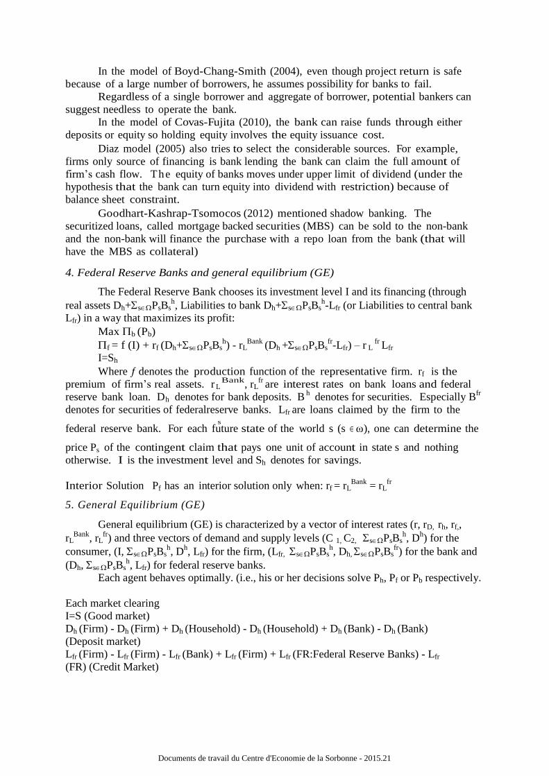
4. Federal Reserve Banks and general equilibrium (GE)
The Federal Reserve Bank chooses its investment level I and its financing (through
real assets Dh+sPsBsh, Liabilities to bank Dh+sPsBs
h-Lfr (or Liabilities to central bank
Lfr) in a way that maximizes its profit:
Max b (Pb)
f = f (I) + rf (Dh+sPsBsh) - rL
Bank (Dh +sPsBs
fr-Lfr) – r
L
fr Lfr
I=Sh
Where denotes the production function of the representative firm. rf is the
premium of firm’s real assets. r LBank
, rLfr
are interest rates on bank loans and federal
reserve bank loan. Dh denotes for bank deposits. Bh
denotes for securities. Especially Bfr
denotes for securities of federalreserve banks. Lfr are loans claimed by the firm to the
federal reserve bank. For each future state of the world s (s ∈ ω), one can determine the
price Ps of the contingent claim that pays one unit of account in state s and nothing
otherwise. I is the investment level and Sh denotes for savings.
Interior Solution Pf has an interior solution only when: rf = rLBank
= rLfr
5. General Equilibrium (GE)
General equilibrium (GE) is characterized by a vector of interest rates (r, rD, rh, rf,,
rLBank
, rLfr) and three vectors of demand and supply levels (C 1, C2, sPsBs
h, D
h) for the
consumer, (I, sPsBsh, D
h, Lfr) for the firm, (Lfr, sPsBs
h, Dh, sPsBs
fr) for the bank and
(Dh, sPsBsh, Lfr) for federal reserve banks.
Each agent behaves optimally. (i.e., his or her decisions solve Ph, Pf or Pb respectively.
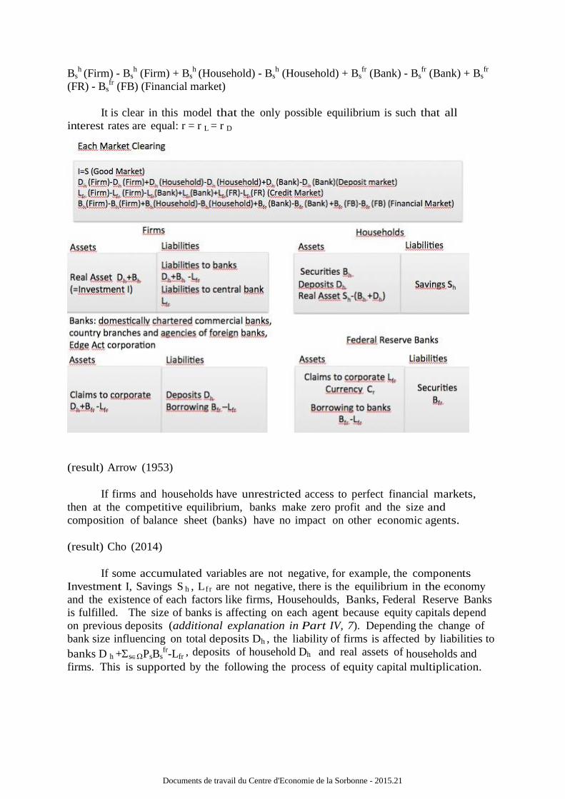
Each market clearing
I=S (Good market)
Dh (Firm) - Dh (Firm) + Dh (Household) - Dh (Household) + Dh (Bank) - Dh (Bank)
(Deposit market)
Lfr (Firm) - Lfr (Firm) - Lfr (Bank) + Lfr (Firm) + Lfr (FR:Federal Reserve Banks) - Lfr
(FR) (Credit Market)
Documents de travail du Centre d'Economie de la Sorbonne - 2015.21
Page 19
Bsh
(Firm) - Bsh (Firm) + Bs
h (Household) - Bs
h (Household) + Bs
fr (Bank) - Bs
fr (Bank) + Bs
fr
(FR) - Bsfr (FB) (Financial market)
It is clear in this model that the only possible equilibrium is such that all
interest rates are equal: r = r L = r D
(result) Arrow (1953)
If firms and households have unrestricted access to perfect financial markets,
then at the competitive equilibrium, banks make zero profit and the size and
composition of balance sheet (banks) have no impact on other economic agents.
(result) Cho (2014)
If some accumulated variables are not negative, for example, the components
Investment I, Savings S h , L f r are not negative, there is the equilibrium in the economy
and the existence of each factors like firms, Househoulds, Banks, Federal Reserve Banks
is fulfilled. The size of banks is affecting on each agent because equity capitals depend
on previous deposits (additional explanation in Part IV, 7). Depending the change of
bank size influencing on total deposits Dh , the liability of firms is affected by liabilities to
banks D h +sPsBsfr-Lfr , deposits of household Dh and real assets of households and
firms. This is supported by the following the process of equity capital multiplication.
Documents de travail du Centre d'Economie de la Sorbonne - 2015.21
Page 20
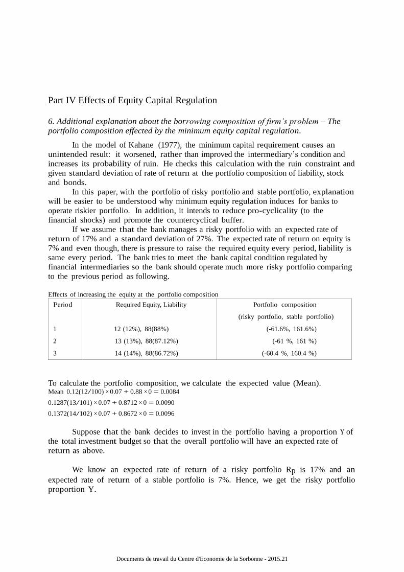
Part IV Effects of Equity Capital Regulation
6. Additional explanation about the borrowing composition of firm’s problem – The
portfolio composition effected by the minimum equity capital regulation.
In the model of Kahane (1977), the minimum capital requirement causes an
unintended result: it worsened, rather than improved the intermediary’s condition and
increases its probability of ruin. He checks this calculation with the ruin constraint and
given standard deviation of rate of return at the portfolio composition of liability, stock
and bonds.
In this paper, with the portfolio of risky portfolio and stable portfolio, explanation
will be easier to be understood why minimum equity regulation induces for banks to
operate riskier portfolio. In addition, it intends to reduce pro-cyclicality (to the
financial shocks) and promote the countercyclical buffer.
If we assume that the bank manages a risky portfolio with an expected rate of
return of 17% and a standard deviation of 27%. The expected rate of return on equity is
7% and even though, there is pressure to raise the required equity every period, liability is
same every period. The bank tries to meet the bank capital condition regulated by
financial intermediaries so the bank should operate much more risky portfolio comparing
to the previous period as following.
Effects of increasing the equity at the portfolio composition
Period Required Equity, Liability Portfolio composition
(risky portfolio, stable portfolio)
1 12 (12%), 88(88%) (-61.6%, 161.6%)
2 13 (13%), 88(87.12%) (-61 %, 161 %)
3 14 (14%), 88(86.72%) (-60.4 %, 160.4 %)
To calculate the portfolio composition, we calculate the expected value (Mean). Mean 0.12(12/100) × 0.07 + 0.88 × 0 = 0.0084
0.1287(13/101) × 0.07 + 0.8712 × 0 = 0.0090
0.1372(14/102) × 0.07 + 0.8672 × 0 = 0.0096
Suppose that the bank decides to invest in the portfolio having a proportion Y of
the total investment budget so that the overall portfolio will have an expected rate of
return as above.
We know an expected rate of return of a risky portfolio Rp is 17% and an
expected rate of return of a stable portfolio is 7%. Hence, we get the risky portfolio
proportion Y.
Documents de travail du Centre d'Economie de la Sorbonne - 2015.21
Page 21
n
n = 0
n = 1
n = 2
n = 3
· · ·
n = k
· · ·
n → ∞
Deposits
D0 = 1
D1 = (1 − β − K)
D2 = (1 − β − K)2
D3 = (1 − β − K)3
· · ·
Dk = (1 − β − K)k
· · ·
D∞ = 0 total
deposits
1 D =
K + β
Borrowings
-
B1 = (1 − β)
B2 = (1 − β)(1 − β − K)
B3 = (1 − β)(1 − β − K)2
· · ·
Bk = (1 − β)(1 − β − K)k−1
· · ·
B∞ = 0
total borrowings
1 − β
K + β
OptimizedEquityCapital
-
OEC1 = K
OEC2 = K(1 − β − K)
OEC3 = K(1 − β − K)2
· · ·
OECk = K(1 − β − K)k−1
· · ·
OEC∞ = 0
total optimized equity capital
K
K + β
Rf + (Rp – Rf)) × Y Proportion Y
0.07 + 0.1 × Y = 0.0084 -0.616
0.07 + 0.1 × Y = 0.0090 -0.61
0.07 + 0.1 × Y = 0.0096 -0.604
Thus, in order to obtain a mean return of 0.84%, 0.90%, 0.96%, the bank must
invest -61.6%, -61%, -60.4 of total funds in the risky portfolio and 161.6%, 161%,
160.4% in stable portfolio.
Standard deviation that implies the probability, to get mean of returns, is also
increasing.
Standard Deviation
0.12 × 0.27 = 0.0324
0.13 × 0.27 = 0.0351
0.14 × 0.27 = 0.0378
7. Previous deposit affects optimized equity capital
B =
[β = restriction of borrowing] Then, Borrowings can be executed between Deposit 1 and
Restriction β
[Balance sheet equality constraint] Dn = Bn – OECn
Hart and Jaffee (1974) analyzed the properties of the feasible and efficient set with the
assumption that the initial equity capital is zero (i.e. K=0). However, it is possible that the
intermediary’s equity is zero in the substantial degree of leverage (high liabilities to equity
ratios 𝐸𝑞𝑢𝑖𝑡𝑦𝐶𝑎𝑝𝑖𝑡𝑎𝑙
𝐷ℎ+𝐵𝑓𝑟+𝐿𝑓𝑟). Then, we should assume that the equity is negliglible.
In the paper as the same as KAHANE (1977), we assume the equity is positive (K 0) so
that the opportunity set does not pas through the origin (i.e. the vector of Deposit D, Borrowing B,
Optimized Equity Capital = 0 give an infeasible solution).
Then theoretical superior limit for deposits is defined by the following:
Documents de travail du Centre d'Economie de la Sorbonne - 2015.21
Page 22
Deposits =
n=0 (1-K-) = 1
𝐾+
Theoretically, superior limit for the equity capital by the firm is defined by the following:
OptimizedEquityCapital = K × Deposit = 𝐾
𝐾+
And the theoretical superior limit for total borrowings in banks is defined by the following:
Borrowings = (1-) × Deposits = 1−
𝐾+
The process described above by the geometric series can be represented, where
Borrowings at stage k are a function of deposits at the precedent stage:
Optimized Equity Capital at stage k is a function of the deposits at the precedent stage:
OECk = K × Dk−1
Hence, if the optimized equity capital depends on the initial deposit and assume the
terminal condition of bank is liquidation of bank deposits.
(result) Hence, Optimized Equity Capital depends on the previous deposit. In addition,
deposit insurance cost also increases because deposit insurance depends on the number of
household.
Deposits at stage k are the difference between additional borrowings and
optimized equity capital relative to the same stage: Dk = Bk − OECk
In the model of Gorton-Winton (1995), bank size is given. In the theorem of
Modigliani-Miller, the size and composition of banks’ balance sheets have no impact on
other agents. However, as population grows, insured deposits will increase. Then, the
bank size should grow so bank size growth concern should be measured.
8. K index for the indicator of risk taking
Define the equity capital ratio with respect to total liabilities and equity capital, 𝐸𝑞𝑢𝑖𝑡𝑦𝐶𝑎𝑝𝑖𝑡𝑎𝑙
𝐷ℎ+𝐵𝑓𝑟−𝐿𝑓𝑟, K(0,1), the borrowing (from federal banks) ratio
𝐵𝑓𝑟−𝐿𝑓𝑟
𝐷ℎ+𝐵𝑓𝑟−𝐿𝑓𝑟, (0,1).
Suppose the demand for funds is unlimited, by summing up two quantities, the
theoretical equity capital multiplier is defined as:
k = 𝐷𝑒𝑝𝑜𝑠𝑖𝑡𝑠+𝑂𝑝𝑡𝑖𝑚𝑖𝑧𝑒𝑑𝐸𝑞𝑢𝑖𝑡𝑦𝐶𝑎𝑝𝑖𝑡𝑎𝑙
𝐵𝑜𝑟𝑟𝑜𝑤𝑖𝑛𝑔𝑠+𝑂𝑝𝑡𝑖𝑚𝑖𝑧𝑒𝑑𝐸𝑞𝑢𝑖𝑡𝑦𝐶𝑎𝑝𝑖𝑡𝑎𝑙 =
1+𝐾
𝐾+
where the equity capital ratio with respect to total liabilities and equity capital, 𝐸𝑞𝑢𝑖𝑡𝑦𝐶𝑎𝑝𝑖𝑡𝑎𝑙
𝐷ℎ+𝐵𝑓𝑟+𝐿𝑓𝑟
k is the index to decline to increase the risk at the portfolio of commercial banks. The
deposit is fixed at total 1 and borrowings have the constraint cannot be negative value beyond the
minimum borrowings . For example, if deposit=1, the minimum of required equity = 10%,
borrowings = 0.3.
Documents de travail du Centre d'Economie de la Sorbonne - 2015.21
Page 23
1+0.1
0.3+0.1 =
1.1
0.4 = 2.75
If the minimum of required equity is raised from 10% to 15%, k index was as below:
1+0.15
0.3+0.15 =
1.15
0.45 = 2.55
To increase the k index, the bank should increase the deposit beyond the initial
deposit level (1 in this simulation) or allocate the borrowing portfolio.
9. Conclusion
The minimum capital requirement is a necessary condition for banking sector
stability to raise the quality, consistency and transparency of the capital base. However,
it has friction with the portfolio management. By using effects of increasing the equity
at the portfolio composition, reducing pro-cyclicality (to the financial shocks) and
promoting the countercyclical buffer are pursued.
In the Basel 3 system, the risk coverage framework intends to capture all material
risks by using counterparty credit risk formula weighted on the external rating of the
counter party. Exposure measures contain on-balance sheet, repurchase agreements and
securities finance, derivatives and off-balance sheet (OBS) items. In the paper, rather
than enlarging the risk contagion, related factors and risk affection scope are detected
without overstatement by using the general equilibrium (GE) model and deposit
affection to the optimized equity capital. Deposits are in the large portion at the
household, firm and banks. To explain risk coverage, by proving correlation of
optimized equity capital upon the previous deposit level, the paper aims to ensure that
banking-sector- capital requirements take account of the macro-financial environment in
which each substantial economic entity operates.
Basel 3 introduced a minimum leverage ratio. The leverage ratio was calculated
by dividing Tier1 capital by the bank’s average total consolidated assets. In the paper, k
index is suggested as the indicator of risk taking. Within the liability, three major
fractions like deposits, borrowings and optimized equity capital are considered as the
complementary of minimum capital requirement. Assets of commercial banks are mainly
consisted with loans and securities. Because the optimized equity capital grows and
deposits is restricted by change. Borrowings that are the difference between asset and
deposit+equity capital should be checked whether borrowings cover the optimized equity
by k index or not.
The combination of portfolio composition test, deposit-equity optimization and k
index enables bounding the bank capital regulation problems.
Documents de travail du Centre d'Economie de la Sorbonne - 2015.21
Page 24
10. Reference
Boyd, J., Chang, C. and Smith, B. (2004). Deposit insurance and bank regulation in a monetary economy: a
general equilibrium exposition. Economic Theory, 24(4), pp.741-767.
Bullard, J. and Waller, C. (2004). Central Bank Design in General Equilibrium. Journal of Money, Credit, and
Banking, 36(1), pp.95-113.
Christensen, I., Meh, C. and Moran, K. (n.d.). Bank Leverage Regulation and Macroeconomic Dynamic. SSRN
Journal.
Covas, F., Fujita, S. (2010). Procyclicality Of Capital Requirements In a General Equilibrium Model of
Liquidity Dependence, International Journal of Central Banking. P.143, P.161.
Dewatripont, M. and Tirole, J. (2012). Macroeconomic Shocks and Banking Regulation. Journal of Money,
Credit and Banking, 44, pp.237-254.
Diamond, D. and Dybvig, P. (1983). Bank Runs, Deposit Insurance, and Liquidity. Journal of Political
Economy, 91(3), p.401.
Diaz, R. A. (2005) General Equilibrium Implications Of The Capital Adequacy Regulation For Banks.
P.12. P.15, P.26.
European Central Bank. 2.5 Deposits held with MFIs. retrieved from
http://sdw.ecb.europa.eu/reports.do?node=100000145.
Freixas, X. (1997). Microeconomics of banking. Cambridge, Mass.: MIT Press.
Goodhart, C., Kashyap, A., Tsomocos, D. and Vardoulakis, A. (n.d.). Financial Regulation in General
Equilibrium. SSRN Journal.
Gorton, G. and Pennacchi, G. (1990). Financial Intermediaries and Liquidity Creation. The Journal of Finance,
45(1), pp.49-71.
Haslag, J. H. (2001) On Fed Watching And Central Bank Transparency In An Overlapping Generations
Model. Federal Reserve Bank Of Dallas. P.5.
Jenter, D. (2003) MIT Sloan Lecture Notes, Finance Theory II.
Kahane, Y. (1977). Capital adequacy and the regulation of financial intermediaries. Journal of Banking &
Finance, 1(2), pp.207-218.
Kaufman, G. G, Scott, K. E (2003) What Is Systemic Risk, and Do Bank Regulators Retard or
Contribute to it?. the Independent Review, P.171. Hendricks, D. (2009) Defining Systemic Risk,
Briefing Paper No1. the Pew Financial Reform Project.
Kemmerer, D., Friedman, M. and Schwartz, A. (1964). A Monetary History of the United States, 1867-1960.
The American Historical Review, 70(1), p.195.
Kim, J. (2011). Milestones About Financial Risk and Basel 3. Korea Reserve Bank, Seoul. South Korea.
retrieved from http://public.bokeducation.or.kr/ecostudy/fridayView.do?btNo=4553.
Krugman, P. and Wells, R. (2006). Economics. New York: Worth Publishers.
Lucas, D. (1995). Comment on Financial Intermediation and Monetary Policy in a General Equilibrium Banking
Model. Journal of Money, Credit and Banking, 27(4), p.1316.
Modigliani, F., Miller, M. (1958) The Cost of Capital, Corporation Finance and the Theory of
Investment. American Economic Review. P.261-297.
Nelson, B., Pinter, G. (2012) Macroprudential Capital Regulation In General Equilibrium. P.14.
Nuno, G., Thomas, C. (2013) Bank Leverage Cycles. P.7. H6.Money Stock Measures. retrieved from
http://www.federalreserve.gov/releases/h6/.
Slovik, P., Cournède, B. (2011) Macroeconomic Impact of Basel III. OECD Economic Department
Working Papers. OECD publishing.
Thaler, R. H. (1997) Irving Fisher: The modern Behavioral Economist. American Economic Review.
VanHoose, D. (2010). The industrial organization of banking. Berlin: Springer.
Documents de travail du Centre d'Economie de la Sorbonne - 2015.21