General rights Copyright and moral rights for the publications made accessible in the public portal are retained by the authors and/or other copyright owners and it is a condition of accessing publications that users recognise and abide by the legal requirements associated with these rights.

Users may download and print one copy of any publication from the public portal for the purpose of private study or research.

You may not further distribute the material or use it for any profit-making activity or commercial gain

You may freely distribute the URL identifying the publication in the public portal If you believe that this document breaches copyright please contact us providing details, and we will remove access to the work immediately and investigate your claim.

Downloaded from orbit.dtu.dk on: Mar 23, 2020

The Barkhausen Criterion (Observation ?)

Lindberg, Erik

Published in:Proceedings of NDES 2010

Publication date:2010

Document VersionPublisher's PDF, also known as Version of record

Link back to DTU Orbit

Citation (APA):Lindberg, E. (2010). The Barkhausen Criterion (Observation ?). In Proceedings of NDES 2010 (pp. 15-18).Dresden, Germany.

The Barkhausen Criterion (Observation ?)

Erik Lindberg, IEEE Life memberFaculty of Electrical Eng. & Electronics,

348 Technical University of Denmark,

DK-2800 Kongens Lyngby, Denmark

Email: el@elektro.dtu.dk

Abstract—A discussion of the Barkhausen Criterionwhich is a necessary but NOT sufficient criterion for steadystate oscillations of an electronic circuit. An attempt toclassify oscillators based on the topology of the circuit.Investigation of the steady state behavior by means of thetime-varying linear approach (”frozen eigenvalues”).

I. INTRODUCTION

Oscillators occur all over in nature and in man-

made systems. Their behavior is characterized by size

(amplitude) and period (frequency). They are controlled

by the basic principle of nature which says that a system

always try to go to a minimum energy state. We observe

oscillators varying in size from 1e+31 for the galaxies in

space to 1e−31 for the super-strings proposed in physics.

Steady state oscillations may be limit cycle oscillations

or chaotic oscillations.

Autonomous oscillators are non-linear oscillating sys-

tems which are only influenced by a constant energy

source. When two oscillating systems are coupled they

try to synchronize in order to obtain the minimum energy

state.

Electronic oscillators are man-made non-linear circuits

which show steady state oscillating behavior when pow-

ered only by dc power supplies. The behavior may be

limit cycle behavior or chaotic behavior. The order of the

circuit is the number of independent memory elements

(capacitive, inductive or hysteric).

For many years we have seen that some basic circuit

theory textbooks introduce the Barkhausen Criterion as

the necessary and sufficient criterion for an electronic

circuit to be an oscillator. Also the concept of linearsteady state oscillators is introduced. The aim of this

discussion is to point out that steady state oscillators

must be non-linear circuits and linear oscillators are

mathematical fictions.

In some textbooks you may also find statements like:

“an oscillator is an unstable amplifier for which the non-linearities are bringing back the initial poles in the right

Fig. 1. Barkhausen’s original observation

half plane of the complex frequency plane, RHP, to theimaginary axis”. This statement is not true [1]. When

you solve the implicit non-linear differential equations

modeling an electronic circuit the kernel of the numerical

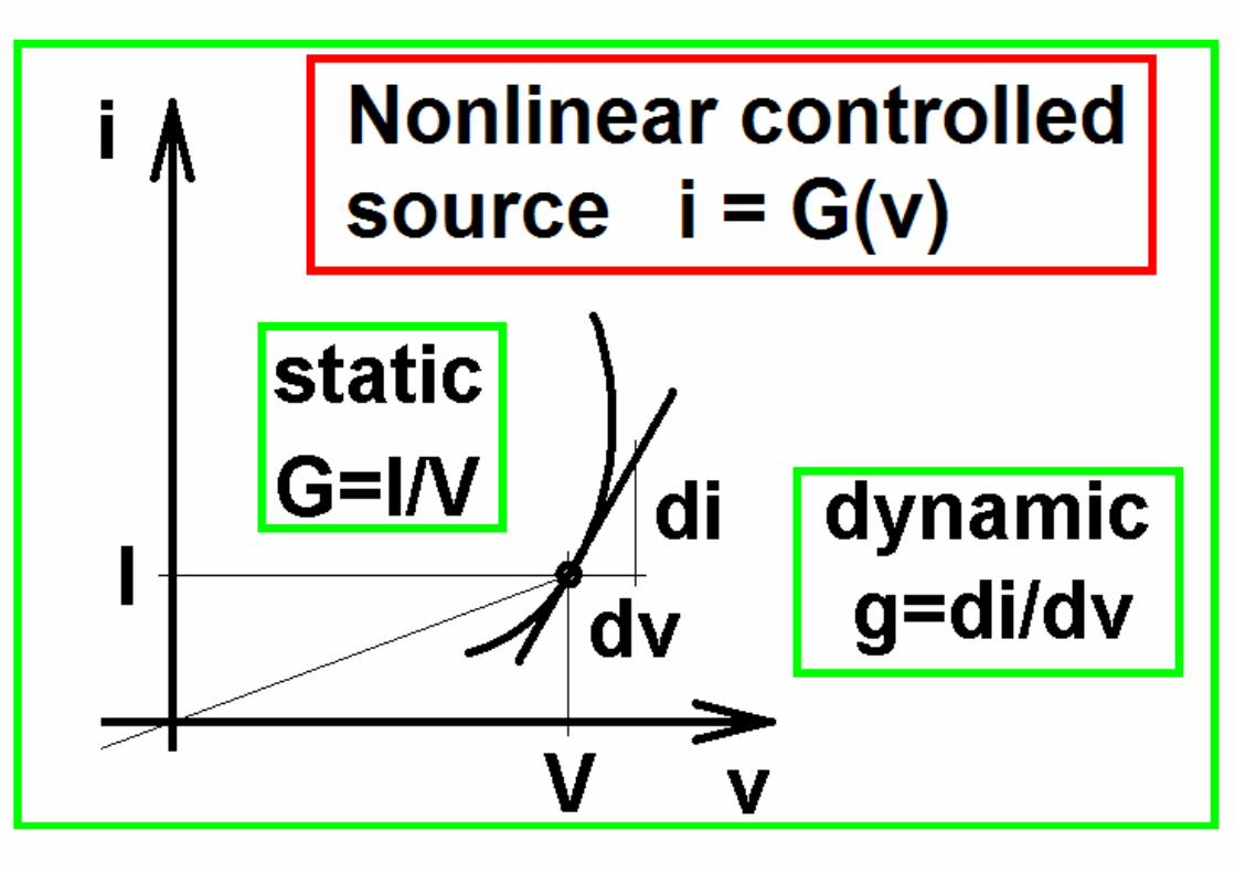
method is the solution of a linear circuit. By means of

Taylor evaluation the nonlinear components are replaced

with linear approximations and iteration is performed

until a solution is obtained. The iteration is based on

Picard (static) or Newton-Raphson (dynamic) methods.

In each integration step a small-signal model is found

for the circuit corresponding to a linearization of the

Jacobian of the differential equations.

Non-linear circuits may be treated as time-varyinglinear circuits so it make sense to study the eigenvaluesas function of time in order to better understand themechanisms behind the behavior of an oscillator.

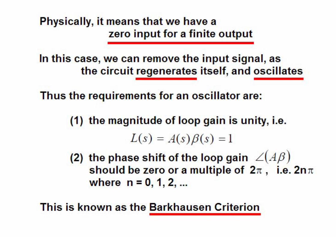
II. BARKHAUSEN’S OBSERVATION

In 1934 H. Barkhausen (1881-1956) [2] pointed out

that an oscillator may be described as an inverting ampli-

18th IEEE Workshop on Nonlinear Dynamics of Electronic Systems (NDES2010)

26-28 May 2010, Dresden, Germany 15

fier (a vacuum tube) with a linear frequency determining

feedback circuit (fig. 1). The non-linear amplifier is

a two-port with a static gain-factor equal to the ratio

between the signals at the ports. The linear feedback

circuit is a two-port with a feed-back-factor equal to

the ratio between the port signals. It is obvious that

the product of the two factors becomes equal to one.

The product is called the Barkhausen Criterion or the

Allgemeine Selbsterregungsformel in German language.

Fig. 2. Barkhausen’s Criterion. Characteristic polynomial

Barkhausens figure may be redrawn as shown in

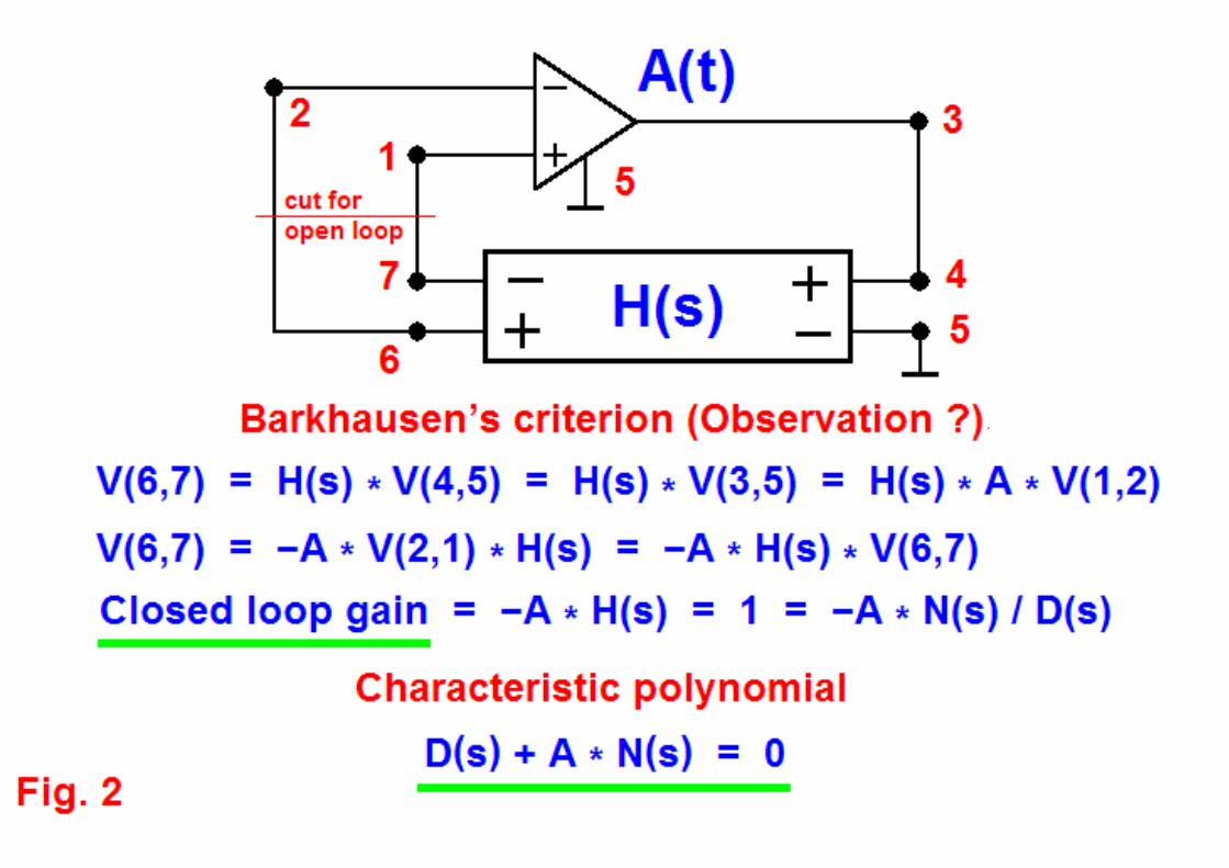
fig. 2 where the non-linear amplifier is assumed to

be a perfect amplifier with infinite input impedance,

zero output impedance and linear time-varying gain A.

The feedback circuit is assumed to be a linear, lumped

element, time-invariant passive two-port with a rational

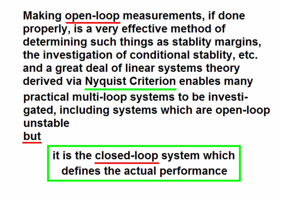
transfer function H(s). It is obvious that the closed-loop

gain is always equal to one (1) and the phase-shift is

equal to a multiple of 360◦ (2π). Furthermore it is seen

that the Barkhausen Criterion is just an expression for

the characteristic polynomial of the circuit as function

of the amplifier gain. For zero gain the characteristic

polynomial becomes equal to the denominator of H(s).

For infinite gain the characteristic polynomial becomes

equal to the numerator of H(s).You may open the loop and study another circuit

closely related to the oscillator circuit. This circuit has

a time independent bias-point. You may perform the

normal linear small-signal analysis (ac analysis) and

study the natural frequencies (poles, eigenvalues). You

may design the open-loop gain to be one (1� 360◦) and

you may also make the closed-loop circuit unstable with

poles in the right half of the frequency plane, RHP, in the

hope that the circuit will start to oscillate. However when

you close the loop the bias-point of the amplifier will

change and you have no guarantee that oscillations start

Fig. 3. Proper Barkhausen topology with H(s) as a modified fullgraph admittance circuit

up. The conclusion is that you must base your design onthe characteristic polynomial of the closed-loop circuit.

Figure 3 shows a realization of the closed-loop circuit

where the feed-back circuit is represented with a mod-

ified full graph admittance circuit. The admittance YE

between node 6 and node 7 is deleted and the admittance

YF between node 4 and node 5 is deleted.

The characteristic polynomial with a full graph

feedback admittance circuit may be found from

Y E × (Y A + Y D + Y C + Y B) +

(Y A + Y B) × (Y D + Y C) +

A × (Y A × Y C − Y B × Y D) = 0 (1)

where the admittances are functions of the complex

frequency s. The admittance YF does not occur because

it is in parallel with the output voltage source of the

amplifier.

The amplifier is a voltage controlled voltage source

(VCVS) and the output signal is returned to the input

by positive (YA, YB) and negative (YC, YD) voltage

division. This structure has been used to investigate

various oscillator families [3], [4], [5].

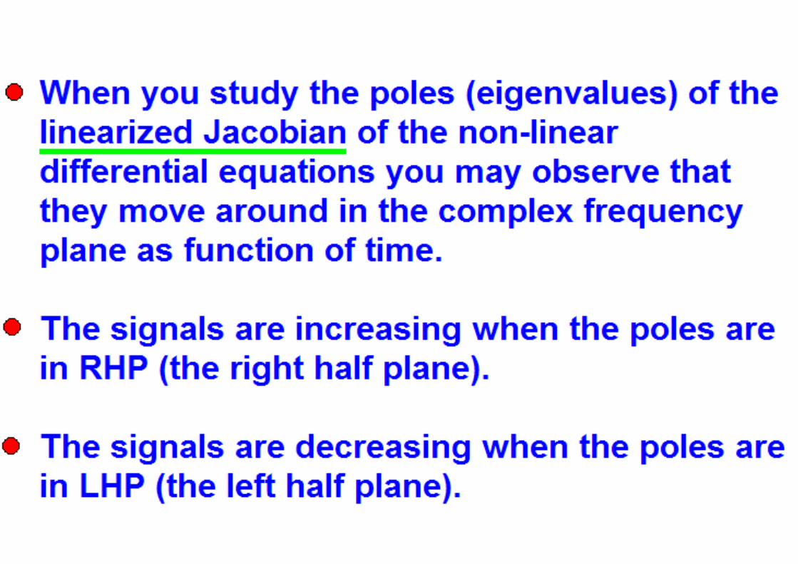
When you study the poles (eigenvalues) of the lin-

earized Jacobian of the non-linear differential equations

you may observe that they move around in the complex

frequency plane as function of time. The signals are

increasing when the poles are in RHP (the right half

plane). The signals are decreasing when the poles are

in LHP (the left half plane). You may observe how a

complex pole pair in RHP goes to the real axis and splits-

up into two real poles of which one goes towards zero

and the other towards infinity. The two real poles meet

again in LHP and leave the real axis as a complex pole

pair [6].

18th IEEE Workshop on Nonlinear Dynamics of Electronic Systems (NDES2010)

26-28 May 2010, Dresden, Germany 16

The basic mechanism behind the behavior of the

oscillator is a balance of the energy received from the

power source when the poles are in RHP with the

energy lost when the poles are in the LHP. The real

part of the poles may go between +∞ and −∞. At

a certain instant the frequency is determined by the

imaginary part of the complex pole pair. The phase noise

observed corresponds to the part of the period where

the instantaneous frequency deviates from the dominant

frequency, the oscillator frequency [7].

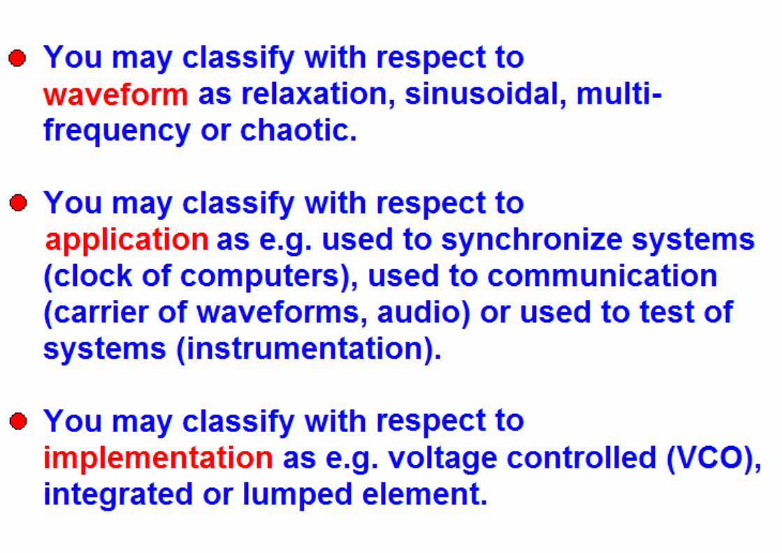
III. CLASSIFICATION OF OSCILLATORS

So far classification of oscillators is not found in

the basic electronics textbooks in a proper way. You

may classify with respect to waveform as relaxation,

sinusoidal, multi-frequency or chaotic. You may classify

with respect to application as e.g. used to synchronize

systems (clock of computers), used to communication

(carrier of waveforms, audio) or used to test of systems

(instrumentation). You may classify with respect to im-plementation as e.g. voltage controlled (VCO), integrated

or lumped element. However a given oscillator may fall

into several of these classes. Classification based on

structure (topology) seems to be the only proper way,

see e.g. [8] where oscillators are classified according to

number of memory elements.

Based on the topology of the circuit oscillators may be

classified as belonging to one of the following classes.

Class I: Proper Barkhausen Topology.

Proper Barkhausen topology is a loop of an amplitude

determining inverting non-linear amplifier and a passive

frequency determining linear feed-back circuit.

The two circuits in the loop are 4-terminal or 3-

terminal two-ports (fig. 1 and fig. 2). The bias point of

the amplifier vary with time.

It is obvious that the power source limits the amplitude

of the oscillator. The following question should be dis-

cussed: Can you separate the design of the non-linearity

from the design of the gain and the linear frequency

determining sub-circuit when designing an oscillator ?

Class II: Modified Barkhausen Topology.

Modified Barkhausen topology is a loop of an in-

verting linear amplifier and a passive amplitude and

frequency determining two-port non-linear feed-back

circuit.

From mathematical point of view a linear amplifier

with constant gain is easy to implement for analysis and

design purposes but a number of questions should be

discussed. Is it possible to create a linear real world am-

plifier which does not influence frequency and amplitude

? Is the dc bias point of the amplifier time-invariant ?

What kind of passive non-linearity should be introduced

in the feed-back circuit ?

Class III: A topology different from I and II, i.e.

non-linear amplifier and non-linear feed-back circuit.

An example of a circuit belonging to this class is the

classic multi-vibrator with two capacitors and two cross-

coupled transistors (3-terminal amplifiers) [4].

In [7] an oscillator based on the differential equations

which have sine and cosine as solutions is investigated.

The oscillator is based on a loop of two active RC

integrators and an inverter. By choosing different time

constants for the two RC integrators phase noise in the

output of one of the amplifiers could be minimized.

IV. AN EXAMPLE TO BE DISCUSSED -

WIEN BRIDGE OSCILLATOR

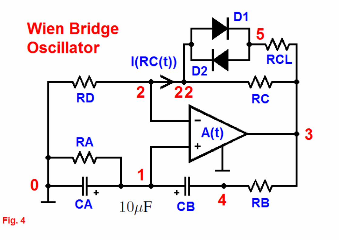
Figure 4 shows a Wien Bridge oscillator with proper

Barkhausen topology (Class I) in the case where resistor

RCL is ∞. The circuit is investigated in [9] where

the operational amplifier is assumed a perfect linear

amplifier with gain A = 100k. The components cor-

Fig. 4. Wien Bridge Oscillator

responding to a complex pole pair on the imaginary axis

are: CA = CB = C = 10nF, RA = RB = R = 20kΩ,

RD = 3kΩ and RC = 6kΩ. The frequency becomes

795.8 Hz and ω0 = 5k rad/sec. The poles of the linear

Wien Bridge oscillator are found as function of resistor

RC . If RC is amended with a large resistor RCL in

series with a non-linear element made from two diodes

in antiparallel as shown in fig. 4 you have a mechanism

for controlling the movement of the poles between RHP

and LHP so you can avoid making use of the non-

linear gain. The circuit becomes a Class II oscillator

with modified Barkhausen topology. For RC = 7kΩ (>6kΩ), D1 = D2 = D1N4148 and three values of

18th IEEE Workshop on Nonlinear Dynamics of Electronic Systems (NDES2010)

26-28 May 2010, Dresden, Germany 17

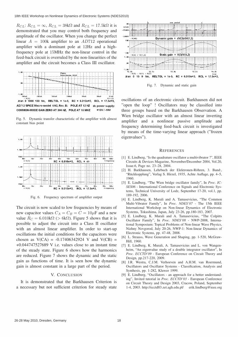
RCL: RCL = ∞, RCL = 38kΩ and RCL = 17.5kΩ it is

demonstrated that you may control both frequency and

amplitude of the oscillator. When you change the perfect

linear A = 100k amplifier to an AD712 operational

amplifier with a dominant pole at 12Hz and a high-

frequency pole at 15MHz the non-linear control in the

feed-back circuit is overruled by the non-linearities of the

amplifier and the circuit becomes a Class III oscillator.

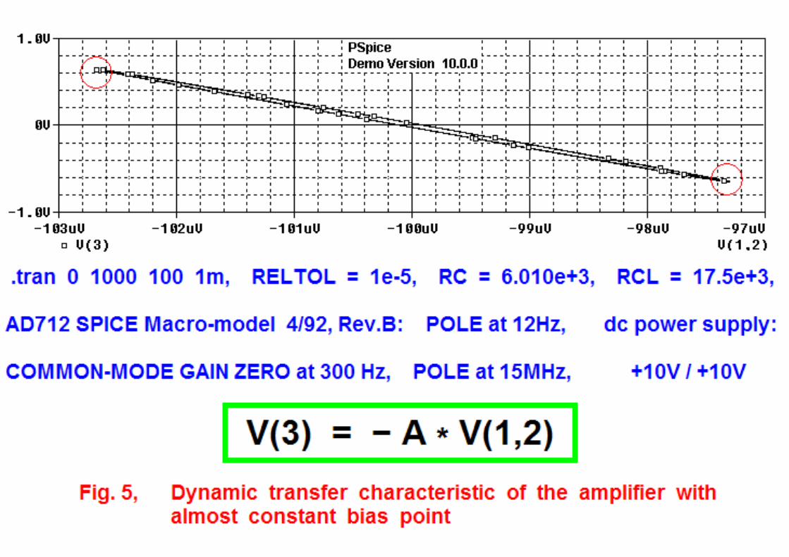
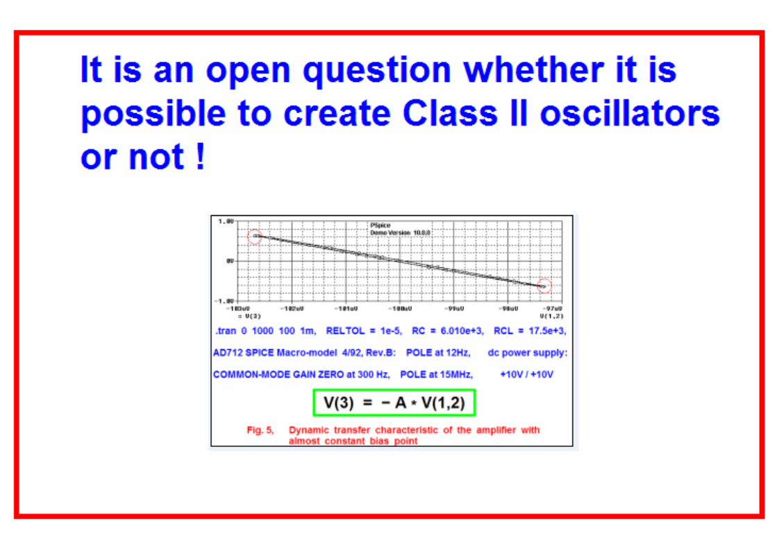
Fig. 5. Dynamic transfer characteristic of the amplifier with almostconstant bias point

Fig. 6. Frequency spectrum of amplifier output

The circuit is now scaled to low frequencies by means of

new capacitor values CA = CB = C = 10μF and a new

value RC = 6.010kΩ (> 6kΩ). Figure 5 shows that it is

possible to adjust the circuit into a Class II oscillator

with an almost linear amplifier. In order to start-up

oscillations the initial conditions for the capacitors were

chosen as V(CA) = -0.17406342924 V and V(CB) =

+0.044747527689 V i.e. values close to an instant time

of the steady state. Figure 6 shows how the harmonics

are reduced. Figure 7 shows the dynamic and the static

gain as functions of time. It is seen how the dynamic

gain is almost constant in a large part of the period.

V. CONCLUSION

It is demonstrated that the Barkhausen Criterion is

a necessary but not sufficient criterion for steady state

Fig. 7. Dynamic and static gain

oscillations of an electronic circuit. Barkhausen did not

”open the loop” ! Oscillators may be classified into

three groups based on the Barkhausen Observation. A

Wien bridge oscillator with an almost linear inverting

amplifier and a nonlinear passive amplitude and

frequency determining feed-back circuit is investigated

by means of the time-varying linear approach (”frozen

eigenvalues”).

REFERENCES

[1] E. Lindberg, “Is the quadrature oscillator a multivibrator ?”, IEEECircuits & Devices Magazine, November/December 2004, Vol.20,Issue.6, Page no. 23–28, 2004.

[2] H. Barkhausen, Lehrbuch der Elektronen-Rohren, 3. Band:,“Ruckkopplung”, Verlag S. Hirzel, 1935, Achte Auflage, pp. 4–5,1960.

[3] E. Lindberg, “The Wien bridge oscillator family”, In Proc. IC-SES06 - International Conference on Signals and Electronic Sys-tems, Technical University of Lodz, September 17-20, vol.1, pp.189-192, 2006.

[4] E. Lindberg, K. Murali and A. Tamasevicius, “The CommonMulti-Vibrator Family”, In Proc. NDES’07 - The 15th IEEEInternational Workshop on Non-linear Dynamics of ElectronicSystems, Tokushima, Japan, July 23-26, pp.180-183, 2007.

[5] E. Lindberg, K. Murali and A. Tamasevicius, “The ColpittsOscillator Family”, In Proc. NDES’08 - NWP-2008, Interna-tional Symposium: Topical Problems of Non-linear Wave Physics,Nizhny Novgorod, July 20-26, NWP-1: Non-linear Dynamics ofElectronic Systems, pp. 47-48, 2008.

[6] L. Strauss, Wave Generation and Shaping, pp. 1-520, McGraw-Hill, 1960.

[7] E. Lindberg, K. Murali, A. Tamasevicius and L. von Wangen-heim, “An eigenvalue study of a double integrator oscillator”, InProc. ECCTD’09 - European Conference on Circuit Theory andDesign, pp.217-220, 2009.

[8] J.R. Westra, C.J.M. Verhoeven and A.H.M. van Roermund,Oscillators and Oscillator Systems - Classification, Analysis andSynthesis, pp. 1-282, Kluwer 1999.

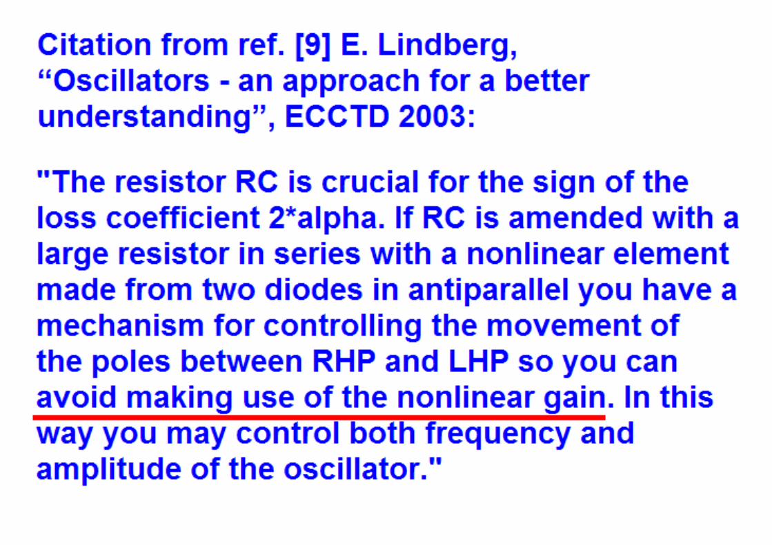
[9] E. Lindberg, “Oscillators - an approach for a better understand-ing”, Invited tutorial in Proc. ECCTD’03 - European Conferenceon Circuit Theory and Design 2003, Cracow, Poland, September1-4, 2003. http://ecctd03.zet.agh.edu.pl/ erik.lindberg@ieee.org

18th IEEE Workshop on Nonlinear Dynamics of Electronic Systems (NDES2010)

26-28 May 2010, Dresden, Germany 18