21
The Basics of Regression Regression is a statistical technique that can ultimately be used for forecasting.
| Date post: | 02-Jan-2016 |
| Category: |
Documents |
| Upload: | halla-sykes |
| View: | 57 times |
| Download: | 0 times |
1
The Basics of Regression
Regression is a statistical technique that can
ultimately be used for forecasting.

2
OverviewIn the section I want to:1) Review the basic idea of inferential statistics,2) Present the elementary information need to understand regression techniques.
In another file I will show you how you can get Microsoft Excel to give you the numbers you need to evaluate relationships between variables. As an example of relationships between variables we might think about how education influences income.
3
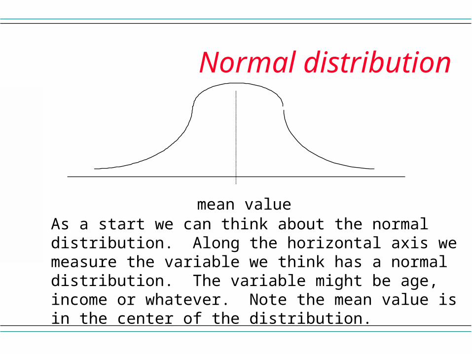
Normal distribution
mean valueAs a start we can think about the normal distribution. Along the horizontal axis we measure the variable we think has a normal distribution. The variable might be age, income or whatever. Note the mean value is in the center of the distribution.
4
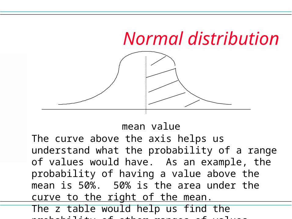
Normal distribution
mean valueThe curve above the axis helps us understand what the probability of a range of values would have. As an example, the probability of having a value above the mean is 50%. 50% is the area under the curve to the right of the mean.The z table would help us find the probability of other ranges of values.
5
ExampleWe could imagine that the people in a typical classroom represent a population. The population would be the people who meet in the class on a regular basis.
As we think of this population, we might want to know about characteristics of the population such as age, income, or educational attainment.
If we looked at the population we would call the population mean and standard deviation of a variable(of say, age) parameters of the population.
6
exampleWhen we look at the people in the class we could find out the population mean by asking everyone to give their age and then we could calculate the mean.
But in many statistical studies we do not collect information from everyone. We only take a sample. The sample will have a mean and standard deviation as well.
Since a sample does not include everyone in the population, the sample mean (and sample standard deviation) will have a value that depends on which people made it into the sample.
7
exampleLet’s take a sample of 5 people in the class and determine the average age. We have ........ .......... ........... ........... ....... for an average of ......................
If we took a different sample of 5 we would have........ .......... ........... ........... ....... for an average of ......................
So in principle we could look at every possible sample of size 5 and calculate the mean for each sample. The mean for each sample of size five could then be looked at as a distribution.
8
sampling distributionWhen we think about repeated sampling, statistics like the mean from the sample could be thought of as a making up a sampling distribution.
Due to the central limit theorem, we know a great deal about the sampling distribution of the sample mean.
The nice thing about the central limit theorem is that it holds whether we know all about the population or not.
9
central limit theoremThe basic idea of the central limit theorem is that if you consider samples from a population, the sampling distribution of sample means 1) has a normal distribution - the sampling distribution is normal, 2) has mean value equal to the mean of the population, and,3) has standard deviation or, in this context, a standard error equal to the standard deviation of the population divided by the square root of the sample size. The standard error is just the standard deviation of the sampling distribution and, as such, is just given this special name.
10
central limit theoremSo we see the variable in the population can have a normal distribution and the sample mean can have a normal distribution.Example: If in the population age ~N(30, 3), then samples of size, say 9, have x ~N(30, 1).
How did I get this? Do you get it?
11
68-95-99.7 ruleFor a normal distribution it is know that 1) approximately 68% of the values are within 1 standard deviation of the mean, 2) approximately 95% of the values are within 2 standard deviations of the mean, and3) approximately 99.7% of the values are within 3 standard deviations of the mean.So from our example of age before, in the population 68% of the people are between 27 and 33, but 68% of the sample means would fall between 29 and 31.
12
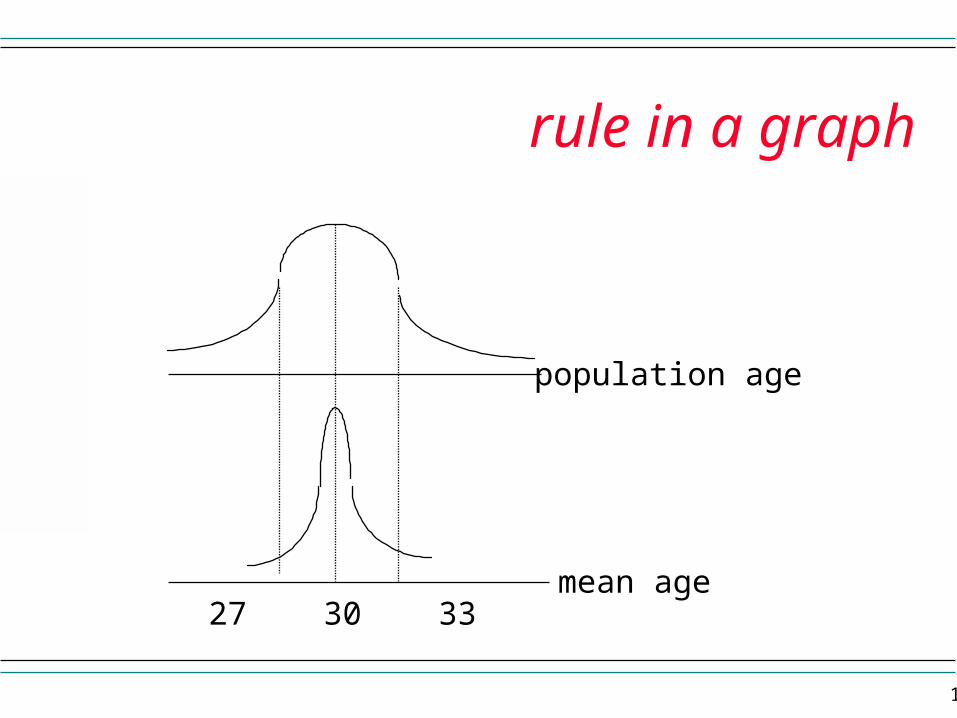
rule in a graph
population age
mean age27 30 33
13
statistical inferenceUp to this point we have operated as if we knew the population mean. (What we have done will act as a model for what we are about to do.) But most of the time we don’t - that is why we have statistics. We will take a sample and try to infer what the population mean is from the sample we draw.The two methods of inference are 1) confidence intervals and2) hypothesis tests.
Let’s briefly look at these for the unknown population mean because the same basic idea applies to regression as well.
14
confidence intervalWhen we take a sample and calculate the mean of the sample we could use this sample mean as our estimate of the population mean. But remember that the mean of the sample would vary depending on the sample. Instead of just a point estimate of the mean of the population we use an interval or range of values for our estimate of where the population mean might be.To account for sampling variability, we use an interval.
15
confidence interval
sample means
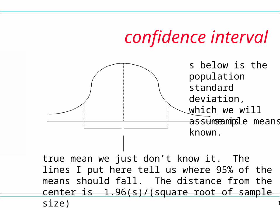
true mean we just don’t know it. The lines I put here tell us where 95% of the means should fall. The distance from the center is 1.96(s)/(square root of sample size)
s below is the population standard deviation, which we will assume is known.
16
confidence interval
sample means
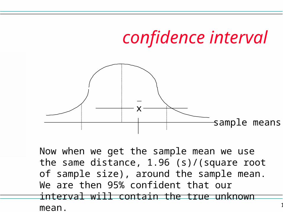
Now when we get the sample mean we use the same distance, 1.96 (s)/(square root of sample size), around the sample mean. We are then 95% confident that our interval will contain the true unknown mean.
x
17
1.96
Where did I get the 1.96 on the previous page? Before we said approximately 95% of the sample means are within 2 standard deviations of the mean. To be more precise we say 95% of the sample means are within 1.96 standard deviations.
If you look at the standard normal table in the book you see associated with a Z = 1.96 the value .475. So .025 is in the upper tail, and due to symmetry, .025 in the lower tail of a normal distribution.
So to be precise we use 1.96 in the formulas when we refer to the middle 95%.
18
Analogy
Say I have a stick and it has a certain length. Also say if I sit in the middle of the room I can whack 95% of you with the stick. This also means that if each of you are given the stick, 95% of you will be able to hit me when I am sitting in the middle.
(Let’s play who can hit the lightest, you go first)
The length of the stick is 1.96 (s)/(square root of sample size), which is sample dependent.
If we were at the true center we could use this stick and “hit 95%” of the values. So if we take a sample and get xbar, then 95% of the time we should be able to “hit” the true center.
19
hypothesis testIn a hypothesis test we don’t know the unknown population mean, but we have a value in mind(the hypothesized value), say from other research or the like. What we then do is use the hypothesized value as if it were the true value and see how likely our sample mean value would be, coming from the population with the center at the hypothesized value. Low probabilities of occurrence(less than 5% or .05) would have us reject our hypothesized value as the true mean.
20
hypothesis test
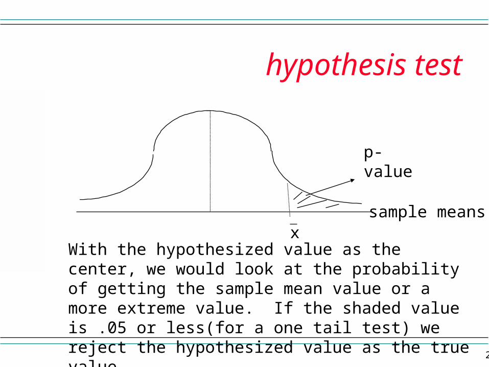
sample means
With the hypothesized value as the center, we would look at the probability of getting the sample mean value or a more extreme value. If the shaded value is .05 or less(for a one tail test) we reject the hypothesized value as the true value.
x
p-value
21
hypothesis test
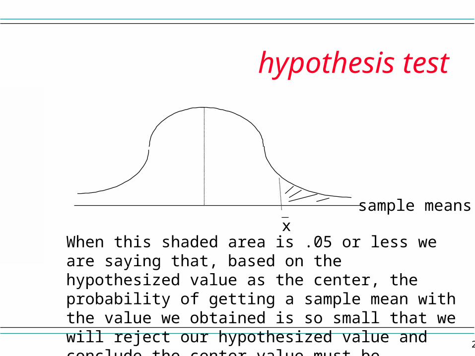
sample means
When this shaded area is .05 or less we are saying that, based on the hypothesized value as the center, the probability of getting a sample mean with the value we obtained is so small that we will reject our hypothesized value and conclude the center value must be something else.
x


