THE BEHAVIOURAL ZLOTY/EURO EQUILIBRIUM EXCHANGE RATE Joanna Bęza-Bojanowska * , Ronald MacDonald ** Abstract Poland is obligated to adopt the euro after the fulfilment, inter alia, of the exchange rate criterion which requires entering the Exchange Rate Mechanism II (ERM II). The European Central Bank recommends that the ERM II central rate should reflect the best possible assessment of the equilibrium exchange rate. In this paper we use the BEER and PEER approach to estimate real Polish zloty/euro equilibrium rate. Although the main goal of our analysis is to compute measures of current and total misalignment, we also check the sensitivity of the equilibrium exchange rate estimates to our choice of the risk premium proxy as well as to our approach for computing the total misalignment. We demonstrate that the BEER/PEER estimates of the PLN/EUR rate are statistically robust and that this approach may be useful for setting the central parity rate at which the zloty enters ERM II. JEL Classification Numbers: F31, F32 Keywords: equilibrium exchange rate, BEER, PEER, cointegration analysis, Gonzalo-Granger decomposition, ERM II * Bureau for Integration with the Euro Area, National Bank of Poland ** Glasgow University
Transcript
THE BEHAVIOURAL ZLOTY/EURO EQUILIBRIUM EXCHANGE RATE
Joanna Bęza-Bojanowska*, Ronald MacDonald**
Abstract
Poland is obligated to adopt the euro after the fulfilment, inter alia, of the exchange rate
criterion which requires entering the Exchange Rate Mechanism II (ERM II). The European
Central Bank recommends that the ERM II central rate should reflect the best possible
assessment of the equilibrium exchange rate. In this paper we use the BEER and PEER
approach to estimate real Polish zloty/euro equilibrium rate. Although the main goal of our
analysis is to compute measures of current and total misalignment, we also check the sensitivity
of the equilibrium exchange rate estimates to our choice of the risk premium proxy as well as to
our approach for computing the total misalignment. We demonstrate that the BEER/PEER
estimates of the PLN/EUR rate are statistically robust and that this approach may be useful for
setting the central parity rate at which the zloty enters ERM II.
4.1. Model specification and data description .................................................................... 9 4.2. Behavioural PLN/EUR equilibrium rate.................................................................... 12 4.3. Permanent PLN/EUR equilibrium rate ...................................................................... 19 4.4. Misalignment analysis ............................................................................................... 23
5. Conclusions ........................................................................................................................ 26 References................................................................................................................................... 27 Annex 1 Main institutional changes in Polish exchange rate regime in the years 1989-2000 .... 31 Annex 2 Data sources and time series plots................................................................................ 32 Source: The authors..................................................................................................................... 33 Annex 3 Econometric analysis outcomes.................................................................................... 34 Chart 1: Recursive test for stability of loading coefficients........................................................ 17 Chart 2: Recursive test for stability of adjustment coefficients .................................................. 18 Chart 3: Current BEER and PEER for real PLN/EUR rate......................................................... 22 Chart 4: Medium-run BEER and PEER for real PLN/EUR rate................................................. 23 Chart 5: Current misalignment.................................................................................................... 25 Chart 6: Total misalignment........................................................................................................ 25 Chart 7: Levels and first differences of the real PLN/EUR rate and its determinants ................ 33 Chart 8: Recursive LR-test of restrictions................................................................................... 36 Chart 9: The comparison of BEERs estimates using different BS proxies .................................37 Chart 10: The comparison of PEERs estimates using different BS proxies................................38 Table 1: Specifications of BEER model for the Polish zloty (based on time series) .................. 12 Table 2. Cointegration test (restricted models) ........................................................................... 14 Table 3: Identification of the long-run structure for real PLN/EUR rate .................................... 14 Table 4: Loadings to Common Trends - VECM01..................................................................... 20 Table 5. Long-Run Impact Matrix - VECM01............................................................................ 20 Table 6: Loadings to Common Trends - VECM02..................................................................... 21 Table 7. Long-Run Impact Matrix - VECM02............................................................................ 21 Table 8. The real PLN/EUR rate misalignment – review of the literature.................................. 26 Table 9: Unit root test ................................................................................................................. 34 Table 10. Multivariate diagnostics .............................................................................................. 34 Table 11: Cointegration test (no weak exogeneity restrictions).................................................. 35 Table 12: Coefficients of VEC models and weak exogeneity test .............................................. 35 Table 13: Common Trends - VECM01....................................................................................... 36 Table 14: Common Trends - VECM02....................................................................................... 37
4
1. Introduction
Since becoming a member of the European Union, Poland has been participating in the 3rd stage
of the Economic and Monetary Union with the status of a country with derogation (European
Union, 2003). That means Poland is obligated to adopt the euro after the fulfilment of the
Maastricht criteria (European Union, 2002), and, inter alia, the exchange rate criterion. Thus, at
some point it will be necessary to abandon the current floating exchange rate regime and enter
the Exchange Rate Mechanism II (ERM II), which requires setting the central parity against the
euro. However, this raises the question of what that central rate should be. In this paper we
argue the rate should be an equilibrium rate and our main focus here is on calculating current
and medium-run Polish zloty/euro (hereafter PLN/EUR) equilibrium rates and the implied
misalignment of the actual PLN/EUR rate from its equilibrium.
Two measures of equilibrium are used in this paper to estimate the equilibrium
PLN/EUR, namely the behavioural equilibrium exchange rate (BEER) model, which is applied
to calculate the current equilibrium exchange rate, and the permanent equilibrium exchange rate
model (PEER) to estimate the medium-run equilibrium exchange rate. In essence the
BEER/PEER approach involves reduced form modelling of the equilibrium exchange rate using
cointegration analysis.
The outline of the remainder of the paper is as follows. In the next section we discuss the
various ways of estimating an equilibrium exchange rate and in Section 3 we go on to present
the econometric methodology used to estimate our preferred measures of the equilibrium
exchange rate, namely the BEER and PEER. Our estimates of these equilibrium measures for
the Polish zloty/euro rate are presented in Section 4 and in Section 5 we give some concluding
remarks.
2. Measuring the Equilibrium Exchange Rate
In this section we outline the methodology of the BEER and PEER approaches to estimating the
equilibrium exchange rate and contrast them with variants of the internal-external balance
approach.
The BEER approach of Clark and MacDonald (1998) is not based on any specific
exchange rate model and in that sense may be regarded as a very general approach to modelling
equilibrium exchange rates. However, it takes as its starting point, though the proposition that
real factors are a key explanation for the slow mean reversion to PPP observed in the data (so-
called PPP puzzle, see Rogoff, 1996). In contrast to some of the FEER based approaches,
5
discussed below, it's specific modus operandi is to produce measures of exchange rate
misalignment which are free of any normative elements and one in which the exchange rate
relationship is subject to rigorous statistical testing.
We follow Clark and MacDonald (1998) and define Z1t as a set of fundamentals which
are expected to have persistent effects on the long-run real exchange rate and Z2t as a set of
fundamentals which have persistent effects in the medium-run, that is over the business cycle.
Given this, the actual real exchange rate may be thought of as being determined in the following
way:
ttT
tT
tT
t TZZq ετββ +++= 221'
1 , (2.1)
where tT is a set of transitory, or short-run, variables and tε is a random error. Following Clark
and MacDonald (1998), it is useful to distinguish between the actual value of the real exchange
rate and the current equilibrium exchange rate, tq . The latter value is defined for a position
where the transitory and random terms are zero:
tT
tT
t ZZq 2111 ββ += . (2.2)
The related current misalignment, cm, is then given as:
ttT
tT
tT
tttt TZZqqqcm ετββ +=−−=−= 2111 , (2.3)
and so cm is simply the sum of the transitory and random errors. As the current values of the
economic fundamentals can deviate from the sustainable, or desirable, levels, Clark and
MacDonald (1998) also define the total misalignment, tm, as the difference between the actual
rate and the rate given by the sustainable or long-run values of the economic fundamentals,
denoted as:
tT
tT
tt ZZqtm 2211 ββ −−= . (2.4)
By adding and subtracting tq from the right hand side of (2.4) the total misalignment can be
decomposed into two components:
)]()([)( 222111 ttT
ttT
ttt ZZZZqqtm −+−+−= ββ , (2.5)
and since ttT
tt Tqq ετ +=− , the total misalignment in equation (2.5) can be rewritten as:
)]()([ 222111 ttT
ttT
ttT
t ZZZZTtm −+−++= ββετ . (2.6)
Expression (2.6) indicates that the total misalignment at any point in time can be decomposed
into the effect of the transitory factors, the random disturbances, and the extent to which the
economic fundamentals are away from their sustainable values.
6
To illustrate their approach, Clark and MacDonald (1998) take the risk adjusted real
interest parity relationship, which has been used by a number of researchers to model
equilibrium exchange rates (see, for example, Faruqee, 1995 and MacDonald, 1998):
ttte
kt rrq λ+−−=∆ + )( * . (2.7)
Since in this paper we express the real exchange rate as the home currency price of a unit of
foreign currency we adjust all equations to this definition. Expression (2.7) may be rearranged
as an expression for the real exchange rate as:
ttte
ktt rrqq λ+−−= + )( * , (2.8)
and if ektq + is interpreted as the ‘long-run’ or systematic component of the real exchange rate,
tq̂ and rearranging (2.8) with rational expectations imposed, we get:
ttttt rrqq λ+−−= )(ˆ * . (2.9)
By assuming that tq̂ is, in turn, a function of net foreign assets, nfa, the Balassa-Samuelson
effect, bs, and the terms of trade, tot, an expression for the real exchange rate may be written as:
],,,,[ *ttttttt bstotnfarrfq λ−= . (2.10)
In practice, the estimated BEER is calculated by linearily summing the cointegrating
vectors and the current misalignment is generated as the difference between the actual real
exchange rate and the BEER (see e.g. Clark and MacDonald, 1998). As the data fundamentals
may be away from their equilibrium values, the total misalignment may substantially differ from
the current misalignment. Clark and MacDonald (1998, 2004) proposed two measures of total
misalignment. In first exercise they suggest to set the NFA position (of the US) at a 'sustainable
level' or to use a simple Hodrick-Prescott filter to remove the business cycle related component
from the data. As an alternative to using a Hodrick-Prescott filter Clark and MacDonald (2004)
propose calculating a total misalignment using the Granger-Gonzalo decomposition of the
VECM (Granger and Gonzalo, 1995) and this labelled the permanent equilibrium exchange rate
(PEER), and is discussed in more detail in the next section.
The internal-external balance (IEB) approach is an alternative and popular way of
estimating an equilibrium exchange rate in which deviations from PPP are explicitly recognised.
In that sense it has some similarities to the BEER approach. However, the key difference with
the BEER approach is that the IEB usually places more structure, in a normative sense, on the
determination of the exchange rate. In particular, and in general terms, the equilibrium real
exchange rate is defined as that rate which satisfies both internal and external balance. Internal
balance is usually taken to be a level of output consistent with full employment and low
7
inflation – say, the NAIRU - and the net savings generated at this output level have to be equal
to the current balance, which need not necessarily equal zero in this approach. The general
flavour of the IEB approach may be captured by the following equation (for more details see,
for example, MacDonald, 2000, 2007):
CAPYqCAXIWS −==− ),ˆ()()( , (2.11)
where S denotes national savings, I denotes investment spending, W, X, Y are vectors of
variables, depending on the model specification1, and q̂ is the real exchange rate consistent
with internal balance and the value chosen for the external balance objective (CAP). All of the
approaches discussed in this part use a variant of this relationship. In the fundamental
equilibrium exchange rate (FEER) of Williamson (1983, 1994) the equilibrium exchange rate is
an explicitly medium-run concept, in the sense that the FEER does not need to be consistent
with stock-flow equilibrium (the medium-run is usually taken to be a period of about 5 years in
the future). The definition of internal balance used in this approach is as given above - high
employment and low inflation and external balance is characterised as the sustainable desired
net flow of resources between countries when they are in internal balance. This is usually
arrived at judgementally, essentially by taking a position on the net savings term in (2.11)
which, in turn, will be determined by factors such as consumption smoothing and demographic
changes. The use of the latter assumption, especially, has meant that the FEER is often
interpreted as a normative approach and the calculated FEER is likely to be sensitive to the
choice of the sustainable capital account. It also means that the misalignment implied by the
FEER is a total misalignment. The NATREX model of Stein (1994, 1999) is also within the
spirit of the IEB approach although, in contrast to the FEER approach, both medium-run and
long-run – stock-flow consistent – measures of the equilibrium exchange rate are calculated and
the equilibrium is estimated using cointegration-based methods which makes the actual measure
of equilibrium similar to the BEER.
3. Econometric methodology
The identification of the long-run relationship between an exchange rate and economic
fundamentals is performed by applying the full information maximum likelihood estimation
1 In the FEER W usually contains budget deficit, domestic output gap, GDP differential and dependency ratio; X is a vector of domestic output gap, GDP differential and dependency ratio; Y consists of domestic and foreign output gap. In the NATREX W in general contains rate of time preference and net foreign assets; X consists of productivity, Tobin’s ‘q’ and capital stock; Y is a vector of Tobin’s ‘q’, capital stock and net foreign assets.
8
procedure proposed by Johansen (1995) to estimate the cointegrated vector error-correction
model (VECM):
tt
K
kktkt
Tt DxxABx ε+Φ+∆Γ+=∆ ∑
−
=−−
1
11 , (3.1)
where the notation is as follows: x is a vector of p variables, B is a matrix of r orthogonal
linearly independent cointegrating vectors between the variables in x , A is an adjustment
matrix to the equilibrium trajectories (loading coefficients), Γ is a matrix of the short-run
coefficients, D is a vector of j deterministic variables, Φ is a matrix of parameters of
deterministic components, ε is a vector of white noise residuals and Pp ,...,2,1= ,
As the data set is limited, the estimation and testing strategy follows that proposed by
Greenslade et al. (2002). In the first stage, the weak exogeneity restrictions were tested and
imposed (the model reduction process), the cointegration rank was then tested and the small
sample Bartlett correction was then applied (Johansen, 2002). In a final stage the identification
of the long-run structure (Gonzalo and Granger, 1995) as well as the recursive test for the
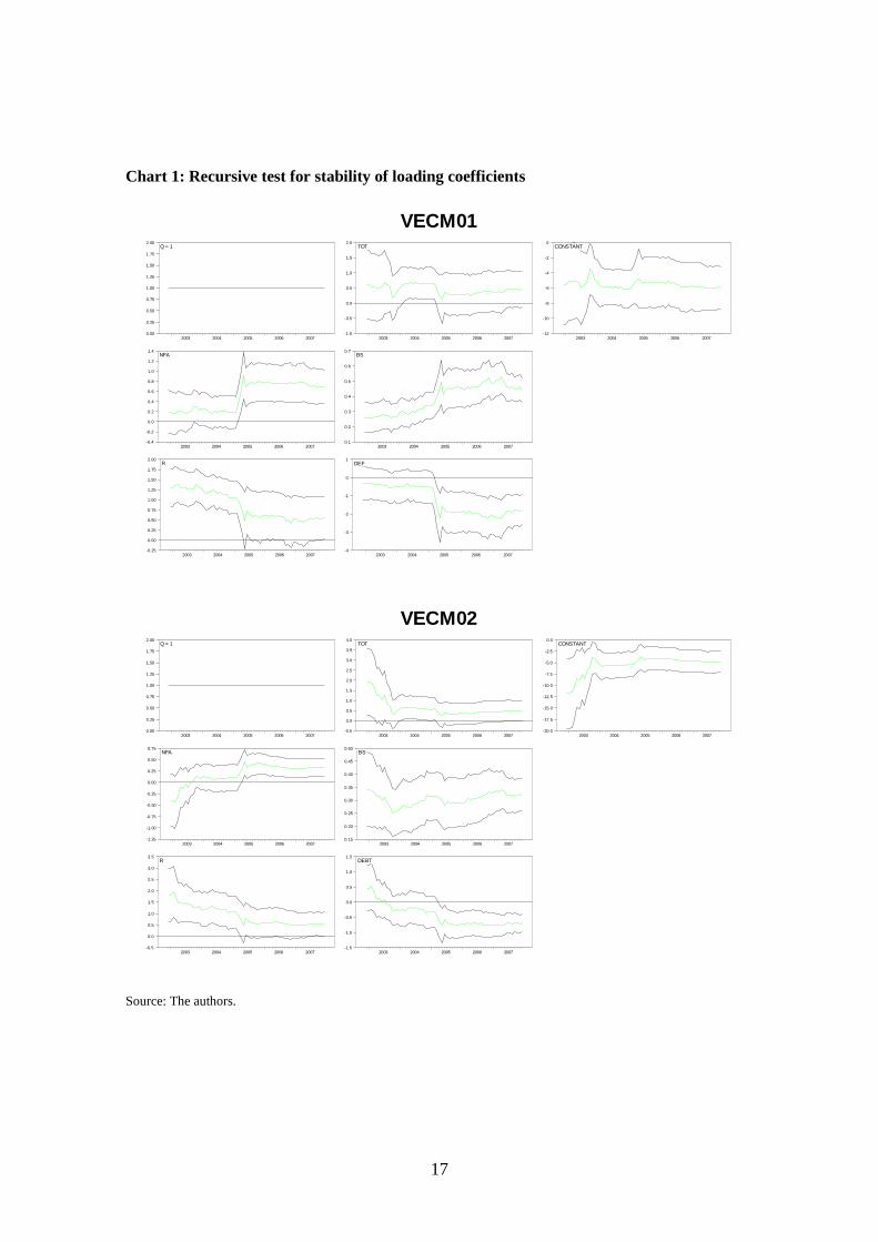
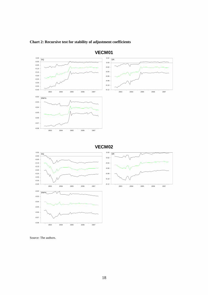
coefficients stability (e.g. Hansen and Johansen, 1999) were performed.
As Johansen (1995) has demonstrated, the above VEC model has a vector moving
representation of the following form:
t
t
ii
t
iit YDCCx +Φ+= ∑∑
== 11
ε (3.2)
where:
TTTC ⊥⊥⊥−
⊥⊥⊥ =Γ= αβαβαβ~
1)( (3.3)
⊥α , ⊥β - orthogonal complements to α and β , respectively,
~
⊥β - loadings to p-r common stochastic trends ∑=
t
ii
1
ε ,
C - the long-run impact matrix.
Granger and Gonzalo (1995) have demonstrated that if the vector tx has a reduced rank
the elements of this vector can be explained in terms of a smaller number n-r of I(1) variables,
tf , called common factors plus some I(0) components, the transitory elements tx~ :
ttt xfAx ~1 += , (3.4)
9
where:
1A - the loading matrix such as 01 =ATα ,
tt xBf 1= ,
11 )( −
⊥⊥⊥= βαβ TA , (3.5)
12 )( −= αβα TA . (3.6)
The identification of the common factors facilitates obtaining the following permanent-
transitory decomposition of tx :
ttt TPx += , (3.7)
where:
tT
t xAP ⊥⊥= βα1 , (3.8)
tT
t xAT β2= . (3.9)
In this paper we intend using the VECM approach of Johansen to obtain BEER estimates for the
zloty and we will use the Granger-Gonzalo approach to calculate the PEER.
4. Real PLN/EUR equilibrium rate
4.1. Model specification and data description
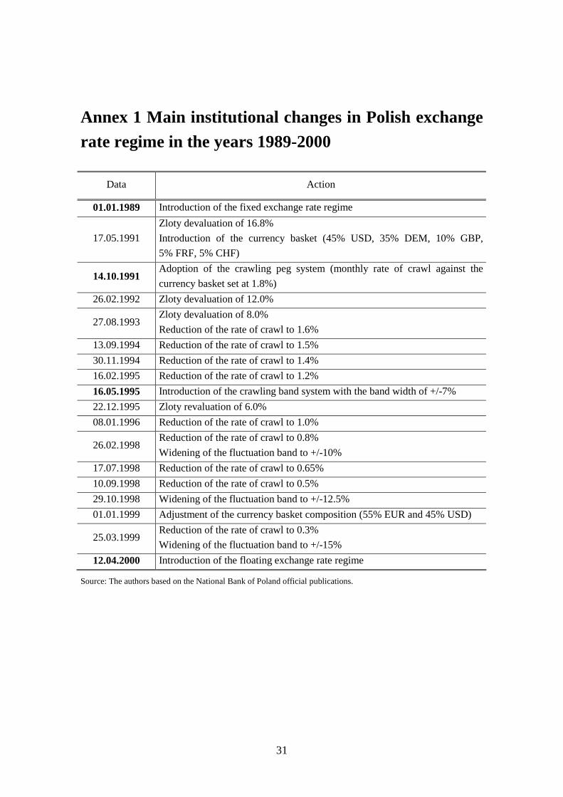
During the transition process the exchange rate regime in Poland evolved from a fixed exchange
rate regime, to a more flexible system with the increasing role of the market in the
determination of the exchange rate, to the pure floating regime that we currently observe (see
International Monetary Fund, 2005). The National Bank of Poland was forced to change
exchange rate regimes due to increasing capital flows, which implied growing sterilization costs
(for more details see Annex 1).
These institutional changes substantially limit the time span of our analysis of the
PLN/EUR equilibrium rate. Since February 1998 was the last large intervention on the Polish
foreign exchange market and the rate thereafter has either been flexible within a crawling band
or fully flexible, we take the period after March 1998 as a homogenously flexible exchange rate
10
regime. For those reasons our monthly data spans the period from March 1998 to December
2007.
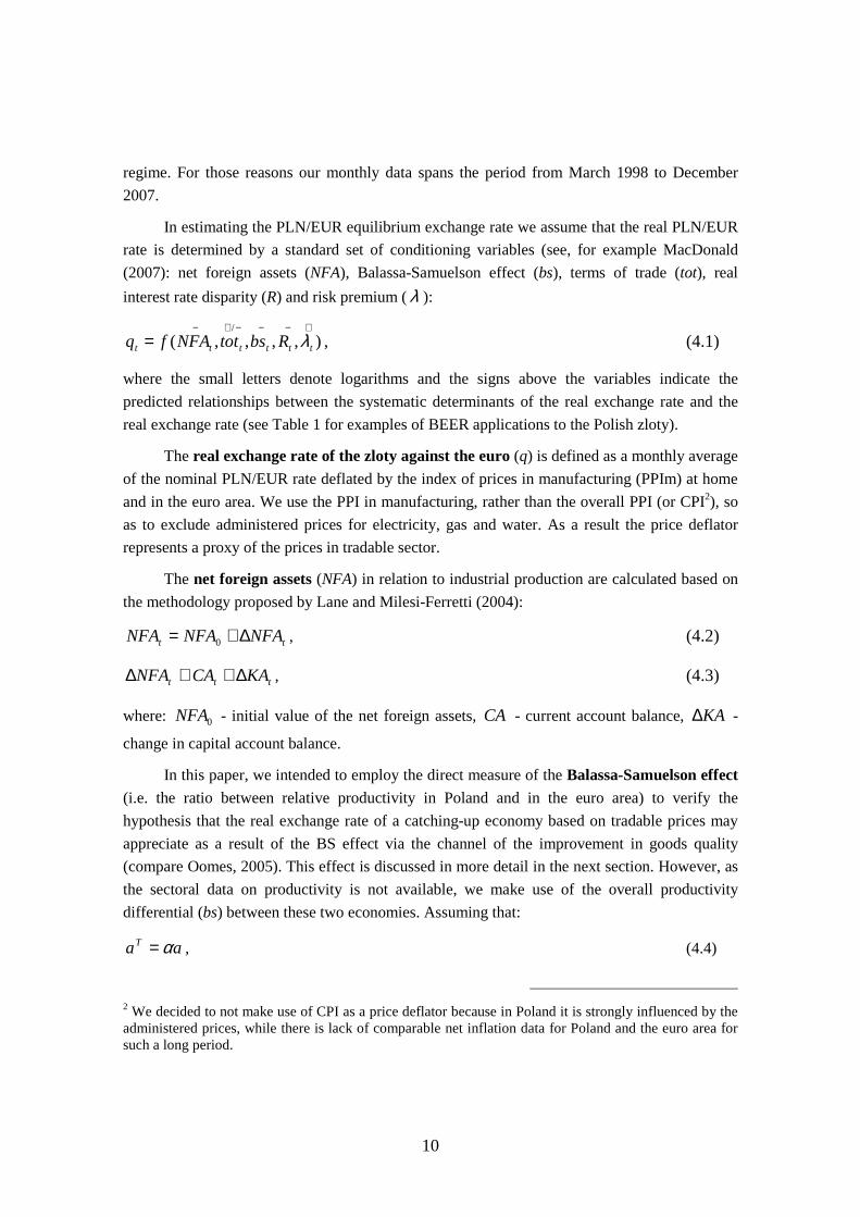
In estimating the PLN/EUR equilibrium exchange rate we assume that the real PLN/EUR
rate is determined by a standard set of conditioning variables (see, for example MacDonald
(2007): net foreign assets (NFA), Balassa-Samuelson effect (bs), terms of trade (tot), real
interest rate disparity (R) and risk premium (λ ):
),,,,(/ +−−−+−
= tttttt RbstotNFAfq λ , (4.1)
where the small letters denote logarithms and the signs above the variables indicate the
predicted relationships between the systematic determinants of the real exchange rate and the
real exchange rate (see Table 1 for examples of BEER applications to the Polish zloty).
The real exchange rate of the zloty against the euro (q) is defined as a monthly average
of the nominal PLN/EUR rate deflated by the index of prices in manufacturing (PPIm) at home
and in the euro area. We use the PPI in manufacturing, rather than the overall PPI (or CPI2), so
as to exclude administered prices for electricity, gas and water. As a result the price deflator
represents a proxy of the prices in tradable sector.
The net foreign assets (NFA) in relation to industrial production are calculated based on
the methodology proposed by Lane and Milesi-Ferretti (2004):
tt NFANFANFA ∆+= 0 , (4.2)
ttt KACANFA ∆+≅∆ , (4.3)
where: 0NFA - initial value of the net foreign assets, CA - current account balance, KA∆ -
change in capital account balance.
In this paper, we intended to employ the direct measure of the Balassa-Samuelson effect
(i.e. the ratio between relative productivity in Poland and in the euro area) to verify the
hypothesis that the real exchange rate of a catching-up economy based on tradable prices may
appreciate as a result of the BS effect via the channel of the improvement in goods quality
(compare Oomes, 2005). This effect is discussed in more detail in the next section. However, as
the sectoral data on productivity is not available, we make use of the overall productivity
differential (bs) between these two economies. Assuming that:
aaT α= , (4.4)
2 We decided to not make use of CPI as a price deflator because in Poland it is strongly influenced by the administered prices, while there is lack of comparable net inflation data for Poland and the euro area for such a long period.
11
aaNT β= , (4.5)
where Ta and NTa denote respectively productivity in tradable and nontradable sector and a is
an overall productivity, then relative productivity grows at rate:
aaa NTT )( βα −=− , (4.6)
which is proportional to overall productivity growth (compare Oomes, 2005).
To check the influence of this assumption on our results, we decided to construct the
second proxy of the BS effect (bstnt), where the tradebles productivity is approximated by the
productivity in manufacturing, while the nontradable productivity growth differential between
Poland and the euro area is assume to be constant and equal to 5%. The higher productivity
growth in the Polish nontradables sector results from foreign direct investment inflows (see e.g.
Alberola, Navia, 2007).
The terms of trade (tot) is defined as a relative ratio between export and import prices in
Poland and Germany. As the corresponding data for the euro area is unavailable, it was assumed
that changes in German terms of trade are representative for the euro area. This assumption
should not have significant impact on the results as the relative terms of trade is to represent
competitiveness of Polish economy and Germany constitutes Polish main trading partner3.
The real interest rate disparity (R) is defined as a difference between monthly average
of 10-year government bond yields for Poland and the euro area, deflated by PPIm.
In order to perform the sensitivity analysis, we also employ different proxies of the risk premium reflecting the fiscal stance of the economy: the budget deficit (DEF) and budget debt (DEBT) in relation to industrial production, respectively. As the monthly data on a
comparable risk premium measure in the euro area is not available, this variable is not expressed
in the relative terms. However, this should not result in the loss of the informativeness of the
data. The risk premium for the zloty denominated investment is determined by the deviation of
the deficit from the reference value (3% of GDP for the general government deficit and 60% of
GDP for the debt; European Union, 2002) and the actions taken by the government in order to
fulfil fiscal criterion rather than its level in the euro area.
For data sources and time series plots see Annex 2.
3 In 2007 Germany accounted for 25,9% of Polish exports and 24,1% of imports.
12
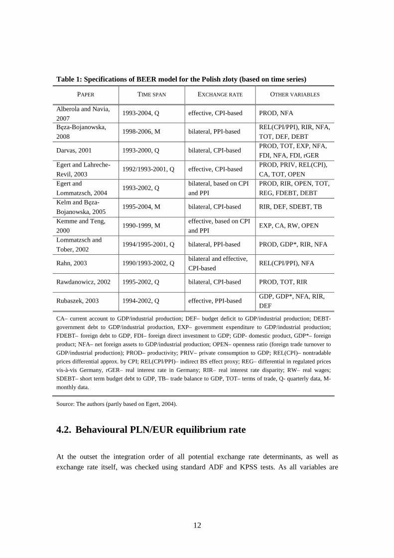
Table 1: Specifications of BEER model for the Polish zloty (based on time series)
prices differential approx. by CPI; REL(CPI/PPI)– indirect BS effect proxy; REG– differential in regulated prices
vis-à-vis Germany, rGER– real interest rate in Germany; RIR– real interest rate disparity; RW– real wages;
SDEBT– short term budget debt to GDP, TB– trade balance to GDP, TOT– terms of trade, Q- quarterly data, M-
monthly data.
Source: The authors (partly based on Egert, 2004).
4.2. Behavioural PLN/EUR equilibrium rate
At the outset the integration order of all potential exchange rate determinants, as well as
exchange rate itself, was checked using standard ADF and KPSS tests. As all variables are
13
integrated of order one (see Table 9 in Annex 3), the VECM methodology was used to estimate
the PLN/EUR equilibrium rate.
In the first stage of the econometric analysis, we estimated two VAR models: VAR01,
with the budget deficit included, and VAR02 with budget debt as an alternative to the budget
deficit4. We jointly specified the deterministic component of the VAR models and the lag
length. This resulted in VAR(2) model and the deterministic component consisting of the
constant and dummies variables5 (necessary to eliminate the residuals skewness). The analysis
of a number of residual diagnostic tests confirms that the estimated VARs are well specified
(see Table 10 in Annex 3). The LM test indicates the lack of significant residual autocorrelation,
while the test for multivariate normality (Doornik and Hansen, 1994) indicates that residuals are
normally distributed; there is also no significant ARCH effect in residuals.
In the next stage, following the proposition of Greenslade et al. (2002), the cointegration
rank test along with the identification of weak exogeneity was performed. The number of
cointegrating vectors was determined by applying the trace test with a Bartlett correction, as
well as the analysis of the largest characteristic roots of the companion matrix (see Table 11 in
Annex 3). The trace test strongly indicates the existence of one cointegrating vector in each
system. The analysis of the number of characteristic roots (Juselius, 2006) confirms the former
finding.
Assuming that cointegration rank equals 1, the long-run relations were determined on the
basis of the Johansen procedure. As the system is to represent the real PLN/EUR equilibrium
rate trajectories, all vectors were normalised on the exchange rate. Three variables (terms of
trade, BS effect and risk premium proxy) proved to be weakly exogenous in each model (see
Table 12 and Chart 8 in Annex 3). The weak exogeneity of these variables is fully in line with
economic reasoning. Poland, as a small open economy, is the price-importer, thus the prices
(terms of trade and BS effect) are not significantly adjusting to the exchange rate equilibrium
trajectory, mainly defined for domestic variables. Moreover, the composition of the
cointegrating vector implies also the weak exogeneity of the risk premium. As the existence of
the weakly exogenous variables may affect the cointegration rank, the cointegration test was
performed once again and the existence of one cointegrating relation was again supported (see
Table 2).
4 As the results proved to be robust to changes in the BS effects proxy, we did not report partial results with the second BS proxy (bstnt). The final outcome, the estimates of the equilibrium exchange rate, is reported in Chart 9-Chart 10 in Annex 3. 5 Dummy variables reflects such effects as: last National Bank of Poland intervention on the foreign exchange market (Jul 98), currency crisis in Russia (Aug-Sep 98), financial and political tensions in Turkey (Jun 01), Polish Prime Minister’s announcement of a risk of financial crisis in Poland (Jul 07), speculation attack on Hungarian forint (Jun 03), tensions on the Hungarian foreign exchange market, decrease in the Hungarian rating (Jun 05).
14
Table 2. Cointegration test (restricted models)
Modulus: 3 largest roots Hypothesis Eigenv. Trace TraceBC Trace*
Finally, we calculate the PEER level and compare it with our BEER estimates (see
Chart 3). The relatively close relation between the BEER and PEER series indicates that the
BEER (especially BEER02) has only a small transitory component. As Clark and MacDonald
(1998, 2004) proved for US the total misalignment may depend significantly on the approach to
computing it. Thus, in order to check whether it is also valid for Polish zloty, we decided to
compute the total misalignment also using the ‘standard’ way, described by the equations (2.4)-
(2.6). In the first variant (labelled BEER HP in Chart 4) we set the long-run values of the
economic fundamentals at the level indicated by the Hodrick-Prescott filter (with the smoothing
22
parameter fixed at the level of 14400; Ravn and Uhlig, 2002). Additionally, we calibrate the
NFA at its optimal level (39% of GDP, European Commission, 2002) and the real interest rate
disparity at the level consistent with the natural interest rates in Poland and in the euro area6,
while the rest of the fundamentals are maintained at the level indicated by HP filter (BEER LT
in Chart 4). However, as the assumptions on the sustainable optimal level of the above listed
variables is fairly strong, we recommend to treat the BEER LT with some caution and we
reported it only for the comparison.
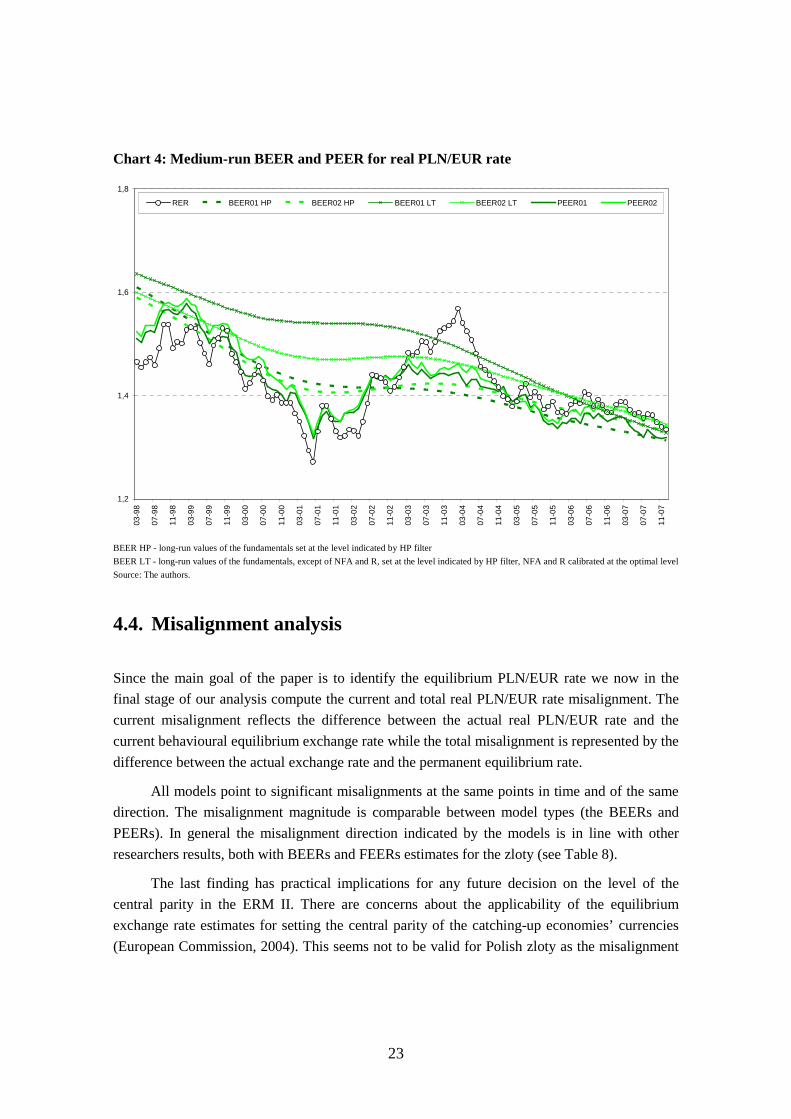
The analysis of Chart 4 indicates that in the past there used to be significant and
persistent differences between the PEER and the medium-run BEER, but since 2003 the relation
between PEER and the latter type of BEER becomes closer, and, what’s more, since EU
accession the misalignment almost disappeared (in case of BEER01 LT since mid-2005). It may
imply that the assumptions on the optimal level of fundamentals are correctly chosen only for
the second half of the analysis horizon.
Chart 3: Current BEER and PEER for real PLN/EUR rat e
1,20
1,40
1,60
1,80
03-9
8
06-9
8
09-9
8
12-9
8
03-9
9
06-9
9
09-9
9
12-9
9
03-0
0
06-0
0
09-0
0
12-0
0
03-0
1
06-0
1
09-0
1
12-0
1
03-0
2
06-0
2
09-0
2
12-0
2
03-0
3
06-0
3
09-0
3
12-0
3
03-0
4
06-0
4
09-0
4
12-0
4
03-0
5
06-0
5
09-0
5
12-0
5
03-0
6
06-0
6
09-0
6
12-0
6
03-0
7
06-0
7
09-0
7
12-0
7
RER BEER01 PEER01 BEER02 PEER02
Source: The authors.
6 The assumptions on the real natural interest rate in Poland (4%) and in the euro area (2%) follow Brzoza-Brzezina (2005).
23
Chart 4: Medium-run BEER and PEER for real PLN/EUR rate
1,2
1,4
1,6
1,8
03-9
8
07-9
8
11-9
8
03-9
9
07-9
9
11-9
9
03-0
0
07-0
0
11-0
0
03-0
1
07-0
1
11-0
1
03-0
2
07-0
2
11-0
2
03-0
3
07-0
3
11-0
3
03-0
4
07-0
4
11-0
4
03-0
5
07-0
5
11-0
5
03-0
6
07-0
6
11-0
6
03-0
7
07-0
7
11-0
7
RER BEER01 HP BEER02 HP BEER01 LT BEER02 LT PEER01 PEER02
BEER HP - long-run values of the fundamentals set at the level indicated by HP filter
BEER LT - long-run values of the fundamentals, except of NFA and R, set at the level indicated by HP filter, NFA and R calibrated at the optimal level
Source: The authors.
4.4. Misalignment analysis
Since the main goal of the paper is to identify the equilibrium PLN/EUR rate we now in the
final stage of our analysis compute the current and total real PLN/EUR rate misalignment. The
current misalignment reflects the difference between the actual real PLN/EUR rate and the
current behavioural equilibrium exchange rate while the total misalignment is represented by the
difference between the actual exchange rate and the permanent equilibrium rate.
All models point to significant misalignments at the same points in time and of the same
direction. The misalignment magnitude is comparable between model types (the BEERs and
PEERs). In general the misalignment direction indicated by the models is in line with other
researchers results, both with BEERs and FEERs estimates for the zloty (see Table 8).
The last finding has practical implications for any future decision on the level of the
central parity in the ERM II. There are concerns about the applicability of the equilibrium
exchange rate estimates for setting the central parity of the catching-up economies’ currencies
(European Commission, 2004). This seems not to be valid for Polish zloty as the misalignment
24
proved to be invariant to the changes in the approach to estimate the equilibrium rate, especially
to switches between BEERs/PEERs and FEERs (see Table 8 for details).
The resulting misalignments for both the BEER and PEER, presented in Chart 5 and
Chart 6, contain several interesting findings:
1. The strong appreciation of the real equilibrium exchange rate, accompanied by an actual
exchange rate appreciation, observed in the years 1998-2001 may be interpreted as a
confirmation of the hypothesis of the natural appreciation of the exchange rate of the
transition country (Halpern and Wyplosz, 1997). This appreciation reflects the adjustment
of the market exchange rate to its equilibrium value that is also in the majority of cases
appreciating (see e.g. Kelm and Bęza-Bojanowska, 2005).
2. It seems that the timing of the introduction of a floating exchange rate regime (April 2000)
was correctly chosen, as the actual exchange rate was close to the actual equilibrium
exchange rate and the total misalignment was rather small. This finding may seem to be
controversial, taking into account high current account deficit at that time. However, if the
relation between the accumulation of the large net foreign liabilities and the production
potential (especially the productivity) is strong, the relationship between the current account
balance and the exchange rate is broken. Thus, in the presence of high current account
deficit, the exchange rate may prove to be fairly valued (compare Alberola, Navia, 2007).
3. In the years 2001-2002, when the PLN/EUR rate reached its historically strongest level, the
zloty was overvalued on average by 3-6% in terms of the current misalignment and 2-3% in
terms of the total misalignment. The magnitude of the misalignment seems to be much
lower that that perceived at that time by various economists.
4. All models unambiguously indicate the highest misalignment in February 2004, amounting
to the zloty undervaluation of 11-16% in terms of the current real equilibrium exchange rate
and of 11-12% for medium-run equilibrium exchange rate. This maximum misalignment
coincides with the historically weak level of the PLN/EUR rate, reached mainly as a result
of political tensions in Poland.
5. Since May 2004 to the end of 2007, the real PLN/EUR rate development was broadly in line
with the current and medium-run equilibrium rate. We observe gradual appreciation of the
equilibrium rate, that was a little bit stronger (especially in 2007) than that of the actual rate.
The appreciation pressure seems to be mainly a result of the BS effect and significant
decrease in risk premium. In this connection, the zloty appreciation in 2008 may be
perceived – to some extent – as a correction of the actual rate towards its equilibrium.
25
Chart 5: C
urrent misalignm
ent
-0,25
-0,20
-0,15
-0,10
-0,05
0,00
0,05
0,10
0,15
0,20
0,25
03-98
07-98
11-98
03-99
07-99
11-99
03-00
07-00
11-00
03-01
07-01
11-01
03-02
07-02
11-02
03-03
07-03
11-03
03-04
07-04
11-04
03-05
07-05
11-05
03-06
07-06
11-06
03-07
07-07
11-07
BE
ER
01
BE
ER
02
So
urce: T
he au
tho
rs.
Chart 6: T
otal misalignm
ent
-0,25
-0,20
-0,15
-0,10
-0,05
0,00
0,05
0,10
0,15
0,20
0,25
03-98
07-98
11-98
03-99
07-99
11-99
03-00
07-00
11-00
03-01
07-01
11-01
03-02
07-02
11-02
03-03
07-03
11-03
03-04
07-04
11-04
03-05
07-05
11-05
03-06
07-06
11-06
03-07
07-07
11-07P
EE
R01
PE
ER
02
So
urce: T
he au
tho
rs.
26
Table 8. The real PLN/EUR rate misalignment – review of the literature
PAPER MODEL PERIOD MISALIGNMENT OUR OUTCOMES
Bęza-Bojanowska,
2008
BEER
PPI-based
Feb 2004
Dec 2006
(+): 12.7-15.9%
close to ER
(+): 10.7-16.6%
close to ER Coudert and
Couharde, 2002
FEER
CPI-based
2000
2001
(-): 7%
(-): 3%
(-): 1-4%
(-): 2-3%
Égert and
Lommatzsch, 2004
BEER
based on CPI and PPI Q4 2002 (-): 12-15% (-): 1%
Lommatzsch and
Tober, 2002
BEER
PPI-based Q4 2001 (-): 10% (-): 3-7%
Rahn, 2003 BEER
CPI-based Q1 2002 (-): 10-15% (-): 6-9%
Rawdanowicz,
2002
FEER
CPI-based 2002 (-): 3.7-6.9% (-): 2-3%
Rubaszek, 2004 FEER
based on GDP deflator Q4 2003 (+): 6.4% (+): 8-9%
(+) – undervaluation, (-) – overvaluation, ER – equilibrium rate
For FEERs totals misalignment was reported (last column)
Source: The authors (partly based on Egert, 2004).
5. Conclusions
Poland is obliged to enter the euro area after the fulfilment of nominal convergence criteria,
which includes participation in the ERM II. This requires abandoning the floating regime and
setting the central parity against the euro. The ECB recommends that the central rate should
reflect the best possible assessment of the equilibrium exchange rate, based on a broad range of
economic indicators while taking into account the market rate (European Central Bank, 2003).
The analysis carried out in this paper focuses on calculating the current and medium-run
real PLN/EUR equilibrium rate while different risk premium proxies are employed. The
objective of the analysis, apart from the assessment of the current situation on the foreign
exchange market, includes the sensitivity analysis of the current and medium-run equilibrium
rate estimates using BEER and PEER approaches.
Applying Johansen’s procedure, two models of the PLN/EUR equilibrium rate were
estimated. Those models differ in the scope of proxies for the risk premium. The results indicate
that net foreign assets, real interest disparity, the terms of trade, the BS effect and the risk
premium determine the real PLN/EUR equilibrium rate. It means the budgetary situation may
play a crucial role for the stability of the PLN/EUR rate in the ERM II.
27
The results of the analysis performed in this paper are encouraging. In particular, the
choice of a risk premium proxy does not affect in any statistically significant way the estimates
of PLN/EUR equilibrium rate (especially permanent rate) or the sources of changes in the
PLN/EUR equilibrium rate. Also the way of calculating total misalignment, i.e. PEER approach
or BEER model based on long-run fundamentals values, does not significantly influence the
assessment of the actual situation on the foreign exchange market. Thus, the presented
approach, especially PEER model, seems to be an appropriate tool for calculating the PLN/EUR
equilibrium rate, which will be taken into account while setting the central parity in the ERM II.
In addition, the fundamentals seem to account for most of the PLN/EUR rate behaviour
while the unexplained movements in the PLN/EUR rate are a measure of the exchange rate
misalignment. All models point to significant misalignments of the same periods, of the same
direction and of a comparable magnitude. The models indicate that since the EU accession, the
real PLN/EUR rate development was broadly in line with the current and medium-run
equilibrium rate with a decrease in the misalignment magnitude and persistence is accompanied
by gradual appreciation of the equilibrium rate. The appreciation pressure seems to result
mainly from the BS effect and a significant decline in the risk premium. As the ERM II entry
should be accompanied by a further drop in the risk premium, we can expect zloty appreciation
within that mechanism. It means that the exchange rate criterion may not be as problematic for
Poland as it used to be perceived and it is probable that Poland will follow the Slovak
experience within ERM II.
References
Alberola, E., D. Navia, 2007, Equilibrium Exchange Rates in the New EU Members: External
Imbalances vs. Real Convergence, Banco de España Working Paper, No. 0708
Bęza-Bojanowska, J., 2008, Behavioural Zloty/Euro Equilibrium Exchange Rate, in Welfe, A.
red., Metody ilościowe w naukach ekonomicznych, Szkoła Główna Handlowa
Brzoza-Brzezina, M., 2005, Lending booms in the new EU Member States: will euro adoption
matter?, European Central Bank Working Papers, No. 543
Clark, P., R. MacDonald, 1998, Exchange Rates and Economic Fundamentals: A
Methodological Comparison of BEERs and FEERs, International Monetary Fund
Working Paper, WP/98/67
Clark, P., R. MacDonald, 2004, Filtering the BEER: A Permanent and Transitory
Decomposition, Global Finance Journal, Vol. 15(1), pp. 29-56
28
Coudert, V., C. Couharde, 2002, Exchange Rate Regimes and Sustainable Parities for CEECs
in the Run-up to EMU Membership, CEPII Working Paper, No. 15
Darvas, Z. 2001, Exchange Rate Pass-Through and Real Exchange Rate in EU Candidate
Countries, Economic Research Centre of the Deutsche Bundesbank Discussion Paper,
No. 10
Doornik, J.A., H. Hansen, 1994, A practical test for univariate and multivariate normality,
Nuffíeld College Discussion Paper
Egert, B., 2004, Assessing Equilibrium Exchange Rates in CEE Acceding Countries: Can We
Have DEER with BEER without FEER? A Critical Survey of the Literature, Bank of
Finland, Institute for Economies in Transition, Discussion Papers, No. 1
Egert, B., A. Lahreche-Revil, 2003, Estimating the Fundamental Equilibrium Exchange Rate
of Central and Eastern European Countries. EMU Enlargement Perspective, CEPII
Working Paper, No. 5
Egert, B., K. Lommatzsch, 2004, Equilibrium Exchange Rates in the Transition: The Tradable
Price-Based Real Appreciation and Estimation Uncertainty, Bank of Finland, Institute for
Economies in Transition, Discussion Papers, No. 9
European Central Bank, 2003, Policy Position of the Governing Council of the European
Central Bank on Exchange Rate. Issues Relating to the Acceding Countries
European Commission, 2002, Public finances in EMU, European Economy No. 3/2002
European Commission, 2004, Discussions on ERM II Participation. Some Guiding Principles,
ECFIN/445/03-EN-Rev1
European Union, 2002, Consolidated Versions of the Treaty on European Union and of the
Treaty Establishing the European Community, Official Journal of the European
Communities, C 325
European Union, 2003, Accession of the Czech Republic, Estonia, Cyprus, Latvia, Lithuania,
Hungary, Malta, Poland, Slovenia and Slovakia, Official Journal of the European
Communities, L 236
Faruqee, H., 1995, Long-Run Determinants of the Real Exchange Rate: A Stock-Flow
Perspective, International Monetary Fund Staff Papers, Vol. 42, No. 1, pp. 80-107
Gonzalo, J., C. Granger, 1995, Estimation of Common Long-Memory Components in
Cointegrated Systems, Journal of Business and Economic Statistics, Vol. 13, No. 1,
pp. 27-35
29
Greenslade, J.V., S.G. Hall, S.G.B. Henry, 2002, On the Identification of Cointegrated
Systems in Small Samples: a modelling strategy with an Application to UK wages and
prices, Journal of Economic Dynamics and Control, Vol. 26, pp.1517-1537
Halpern, L., C. Wyplosz, 1997, Equilibrium Exchange Rates in Transition Economies,
International Monetary Fund Staff Paper, Vol. 44, No. 4, pp. 430-461
Hansen, H., S. Johansen, 1999, Some tests for parameters constancy in the cointegrated VAR,
Econometric Journal, No. 2, pp. 306 – 333
International Monetary Fund, 2005, De Facto Classification of Exchange Rate Regimes and
Monetary Policy Framework as of December 31, 2005
Johansen, S., 1995, Likelihood-based inference in cointegrated vector autoregressive models,
Oxford University Press, Oxford
Johansen, S., 2002, A Small Sample Correction for the Test of Cointegrating Rank in the
Vector Autoregressive Model, Econometrica, Vol. 70, pp. 1929-1961
Juselius, K., 2006, The Cointegrated VAR Model: Methodology and Applications, Oxford
University Press
Kelm, R., J. Bęza-Bojanowska, 2005, Polityka monetarna i fiskalna a odchylenia realnego
kursu złoty/euro od kursu równowagi w okresie styczeń 1995 r. - czerwiec 2004 r.,
National Bank of Poland, Bank i Kredyt, No. 10
Kemme, D., W. Teng, 2000, Determinants of the Real Exchange Rate, Misalignment and
Implications for Growth in Poland, Economic Systems 24(2), pp. 171–205
Lane, P., G. Milesi-Ferretti, 2004, The transfer problem revisited: Net foreign assets and real
exchange rates, The Review of Economics and Statistics, Vol. 86, No. 4, pp. 841-857
Lommatzsch, K., S. Tober, 2002, Monetary Policy Aspects of the Enlargement of the Euro
Area, Deutsche Bank Research Working Paper No. 4
MacDonald, R., 1998, What determines Real Exchange Rates? The Long and Short of It,
Journal of International Financial Markets, Institutions and Money, Vol. 8 (2), pp. 117-
153
MacDonald, R., 2000, Concepts to Calculate Equilibrium Exchange Rates: An Overview,
Economic Research Group of the Deutsche Bundesbank, Discussion Paper 3
MacDonald, R., 2007, Exchange Rate Economics: Theories and Evidence, Taylor & Francis
MacDonald, R., J. Nagayasu, 2000, The long run relationship between real exchange rate and
real interest differential: A panel study, International Monetary Fund Staff Paper,
Vol. 47, No. 1, pp. 116-128
30
Maeso-Fernandez, F., C. Osbat, B. Schnatz, 2001, Determinants of the euro real effective
exchange rate: A BEER/PEER approach, European Central Bank, Working Paper, No. 85
National Bank of Poland, 2007, Międzynarodowa pozycja Polski w 2006 roku
Oomes, N., 2005, Maintaining Competitiveness Under Equilibrium Real Appreciatio: The Case
of Slovakia, International Monetary Fund Working Paper, WP/05/65
Rahn, J., 2003, Bilateral equilibrium exchange rates of EU accession countries against the
euro, Bank of Finland, Institute for Economies in Transition, Discussion Papers, No. 11
Ravn, M., H. Uhlig, 2002, On adjusting the Hodrick-Prescott filter for the frequency of
observations, Review of Economics and Statistics, Vol. 84, No. 2, pp. 371-380
Rawdanowicz, R., 2002, Poland’s accession to EMU - Choosing the parity, Centre for Social
and Economic Research, Studies and Analyses, No. 247
Rogoff, K., 1996, The Purchasing Power Parity Puzzle, Journal of Economic Literature,
Vol. 34, No. 2, pp. 647-668
Rubaszek, M., 2003, Model równowagi bilansu płatniczego. Zastosowanie wobec kursu
złotego. National Bank of Poland, Bank i Kredyt, No. 5
Rubaszek, M., 2004, Modelowanie optymalnego poziomu realnego efektywnego kursu złotego.
Zastosowanie koncepcji fundamentalnego kursu równowagi, National Bank of Poland,
Materiały i Studia, No. 175
Stein, J., 1994, The Natural Real Exchange Rate of the US Dollar and Determinants of Capital
Flows, w J. Williamson ed., 1994, Estimating Equilibrium Exchange Rates, Institute for
International Economics, Washington DC
Stein, J. 1999, The Evolution of the Real Value of the US Dollar Relative To the G7 Currencies,
in R. MacDonald, J. Stein (ed.), 1999, Equilibrium Exchange Rates, Kluwer Academic
Publishers
Williamson, J., 1983, The Exchange Rate System, Institute for International Economics,
Washington DC
Williamson, J., 1994, Estimates of FEERs, in Williamson, J. (ed.) [1994], Estimating
Equilibrium Exchange Rates, Institute for International Economics, Washington DC
31
Annex 1 Main institutional changes in Polish exchange rate regime in the years 1989-2000
Data Action
01.01.1989 Introduction of the fixed exchange rate regime
17.05.1991
Zloty devaluation of 16.8%
Introduction of the currency basket (45% USD, 35% DEM, 10% GBP,
5% FRF, 5% CHF)
14.10.1991 Adoption of the crawling peg system (monthly rate of crawl against the
currency basket set at 1.8%)
26.02.1992 Zloty devaluation of 12.0%
27.08.1993 Zloty devaluation of 8.0%
Reduction of the rate of crawl to 1.6%
13.09.1994 Reduction of the rate of crawl to 1.5%
30.11.1994 Reduction of the rate of crawl to 1.4%
16.02.1995 Reduction of the rate of crawl to 1.2%
16.05.1995 Introduction of the crawling band system with the band width of +/-7%
22.12.1995 Zloty revaluation of 6.0%
08.01.1996 Reduction of the rate of crawl to 1.0%
26.02.1998 Reduction of the rate of crawl to 0.8%
Widening of the fluctuation band to +/-10%
17.07.1998 Reduction of the rate of crawl to 0.65%
10.09.1998 Reduction of the rate of crawl to 0.5%
29.10.1998 Widening of the fluctuation band to +/-12.5%
01.01.1999 Adjustment of the currency basket composition (55% EUR and 45% USD)
25.03.1999 Reduction of the rate of crawl to 0.3%
Widening of the fluctuation band to +/-15%
12.04.2000 Introduction of the floating exchange rate regime
Source: The authors based on the National Bank of Poland official publications.
32
Annex 2 Data sources and time series plots
DATA SOURCES
Real PLN/EUR rate: nominal PLN/EUR rate [NBP7], index of prices in manufacturing in Poland and in the euro area [Eurostat].
Net foreign assets: Poland’s international monetary position [NBP], current account balance [NBP], capital account balance [NBP], industrial production in Poland [CSO8].
Balassa-Samuelson effect: seasonally adjusted index of total industrial production, of production in manufacturing, of employment in total industry, of employment in manufacturing in Poland and in the euro area, respectively [Eurostat].
Terms of trade: export to import prices ratio in Poland [CSO] and Germany [SBD9].
Real interest rate disparity: 10-year government bond yields for Poland and the euro area [Eurostat], index of prices in manufacturing in Poland and in the euro area [Eurostat].
7 National Bank of Poland; www.nbp.pl. 8 CSO - Polish Central Statistical Office; www.stat.gov.pl. 9 SBD - German Federal Statistical Office (Statistisches Bundesamt Deutschland); www.destatis.de. 10 CSO - Polish Central Statistical Office; www.stat.gov.pl.
33
Chart 7: Levels and first differences of the real PLN/EUR rate and its determinants
The table is divided into 2 parts, corresponding to different BEER model specifications. The upper panel of each part reports the normalized vector
estimation: the loading (LT) and the adjustment (ECT) coefficients with t-Student statistics in brackets. The lower panel reports the coefficients of the
restricted model (with weak exogeneity restrictions) and the joint significance level of these restrictions (last column of this table).
Source: The authors.
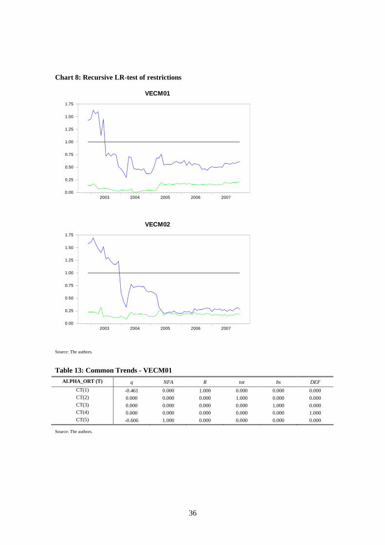
36
Chart 8: Recursive LR-test of restrictions
VECM01
2003 2004 2005 2006 20070.00
0.25
0.50
0.75
1.00
1.25
1.50
1.75
VECM02
2003 2004 2005 2006 20070.00
0.25
0.50
0.75
1.00
1.25
1.50
1.75
Source: The authors.
Table 13: Common Trends - VECM01 ALPHA_ORT (T) q NFA R tot bs DEF