30
The Belousov-Zhabotinsky Oscillator: An Overview By Melody Dodd 10 Dec. 2010

The Belousov-Zhabotinsky Oscillator:An Overview
By Melody Dodd
10 Dec. 2010
A Brief History of Chemical Oscillators
• Have only been recognized as mainstream science since the 1960s.
• Prior belief was that all chemical reactions progressed in one direction (monotonically) to equilibrium.
A Brief History of Chemical Oscillators
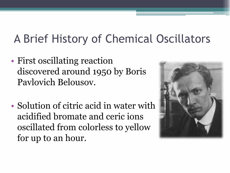
• First oscillating reaction discovered around 1950 by Boris Pavlovich Belousov.
• Solution of citric acid in water with acidified bromate and ceric ions oscillated from colorless to yellow for up to an hour.

A Brief History of Chemical Oscillators
• Belousov’s work ill-received by scientific community.
• Was only recognized posthumously for his contributions.
• Work was continued by Anatol Zhabotinsky in 1961.
• Zhabotinsky succeeded in awakening the scientific community to the validity of chemical oscillators.
• The cerium-bromate reaction became known as the Belousov-Zhabotinsky (BZ) Reaction.

A Brief History of Chemical Oscillators
• Today, many chemical systems are known to oscillate.
• Various mathematical models have been developed to describe the BZ reaction.▫ Brusselator▫ Oregonator
• To date, however, the actual reaction mechanism remains a mystery.

Background: Chemical Kinetics
• Suppose 2 species, A and B, are distributed throughout a domain and are in motion.
• When they come in contact, they form a new species C.
• We can represent this by the chemical equation
.CBA

Background: Chemical Kinetics
• Over time, concentrations of A and B will decrease at the same rate, and the rate of change of C will be the negative of this rate.

Background: Chemical Kinetics
• We can express the rate of change of concentrations of A, B, and C as a dynamical system:
rC
rB
rA
• Intuitively, the reaction rate r depends on the concentrations of A and B.

Background: Chemical Kinetics
• In this simple example, it can be shown that
kABr
where the rate constant k must be determined experimentally.

Background: Chemical Kinetics
• We will now extend this idea to more complicated reactions. Consider
The constants are called the stoichiometric coefficients of the reaction.
A and B are the reactants, C and D are the products.
.DCBA
0,,,

Background: Chemical Kinetics
• We can derive a dynamical system for this reaction using the Law of Mass Action.
• The Law of Mass Action states:
1) The reaction rate r is proportional to the product of the reactant concentrations, with each concentration raised to the power equal to its respective stoichiometric coefficient.
BkAr

Background: Chemical Kinetics
2) The rate of change of the concentration of each species in the reaction is the product of its stoichiometric coefficient with the rate of the reaction, adjusted for sign (+ if product, - if reactant)
rD
rC
rB
rA

Background: Chemical Kinetics
• Thus we arrive at the dynamical system
With known initial concentrations
.
BAkD
BAkC
BAkB
BAkA
.)0(,)0(,)0(,)0( 0000 DDCCBBAA

Modeling The BZ Reaction
• There are many variations on the BZ reaction recipe.
• The recipe that we will demonstrate later contains the following:
Solution Composition
Solution A 0.23M Potassium bromate
Solution B 0.31M Malonic acid,0.059M Potassium bromide
Solution C 0.019M Cerium(IV) ammonium nitrate,2.7M Sulfuric acid
Ferroin Indicator Solution

Modeling The BZ Reaction
• However, our analysis will concern the Oregonator, which is based on a slightly different recipe.
• The Oregonator is considered the simplest model of the BZ Reaction.
• The actual reaction mechanism is extremely complicated; some models have as many as 80 steps and 26 variable species concentrations.

Modeling The BZ Reaction
• Let
• The Oregonator Scheme is then given by the series of 5 reactions:
(Note that the rate constants can be determined empirically).

Modeling The BZ Reaction
• Using the Law of Mass Action, we can derive the following dynamical system:
• We assume that initial concentrations are known.

Modeling The BZ Reaction
• Using nondimensionalization and some simplifying assumptions, we can reduce the system to:
• Note that

Mathematical Analysis
• Taking (based on
empirical data using typical initial concentrations) yields
• As always, the nullclines for this system will be given by
24 104,108,3
2 qf
.
12501
12501
3
50)1(25
zxd
dz
zx
xxx
d
dx
.0,0 d
dz
d
dx

Mathematical Analysis
• We can graph the nullclines and use test points to find flow directions.
• Clearly, there is one positive fixed point
• It can be shown this fixed point will exist for any
).,( ** zx
0, qf

Mathematical Analysis
• Plotting a few trajectories reveals a stable limit cycle.
• Note that the fixed point is clearly unstable.

Mathematical Analysis
• A view of one trajectory with initial conditions close to (0,0).

Mathematical Analysis
• In fact, this system exhibits relaxation oscillations.

Mathematical Analysis
• Question: What effect does varying initial concentrations have on the limit cycle?
• It turns out that this system has a Hopf Bifurcation:
▫ A Hopf Bifurcation is a qualitative change in the phase portrait that occurs as the real parts of eigenvalues of the Jacobian matrix for the system (evaluated at a fixed point) change from negative to positive.
▫ Assuming that q is fixed, we will find that the limit cycle will exist only for certain values of f and ε.
Mathematical Analysis
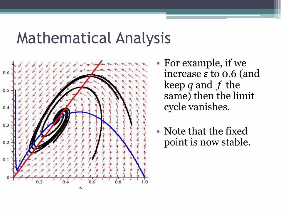
• For example, if we increase ε to 0.6 (and keep q and f the same) then the limit cycle vanishes.
• Note that the fixed point is now stable.

Mathematical Analysis
What values of ε and f will produce oscillations?
1. Compute the positive fixed point by
solving the system to obtain
),( ** zx
0,0 d
dz
d
dx
.**,)26()1(12
1 22* xzqfqfqfx

Mathematical Analysis
2. Compute the Jacobian matrix for the system,
evaluated at the fixed point:
.
11
)(
)(
)(
221
1
),( *
*
2*
**
**
xq
xqf
xq
qfxx
zxJ

Mathematical Analysis
3. The critical value for ε will occur when the real
part of the eigenvalues for the Jacobian matrix are equal to zero. This means the trace of the Jacobian will be zero.
2*
**
2*
**
)(
221
0)(
221
1)(
xq
qfxx
xq
qfxxJtrace

Mathematical Analysis
4. We can graph this result in the ε-f plane to
obtain a region in which oscillations will occur.

References
▫ Gray, Casey R, An Analysis of the Belousov-Zhabotinskii Reaction.
▫ Holmes, M.H., Introduction to the Foundations of Applied Mathematics.
▫ Strogatz, Steven H., Nonlinear Dynamics and Chaos.
▫ Winfree, A.T., The Prehistory of the Belousov-Zhabotinsky Oscillator.


