The Bidder’s Curse Young Han Lee Ulrike Malmendier October 26, 2009 Abstract We employ a novel approach to identify overbidding in the field. We compare auction prices to fixed prices for the same item on the same webpage. In detailed board-game data, 42 percent of auctions exceed the simultaneous fixed price. The result replicates in a broad cross-section of auctions (48 percent). A small fraction of overbidders, 17 percent, su ces to generate the overbidding. The observed behavior is inconsistent with rational behavior, even allowing for uncertainty and switching costs, since also the expected auction price exceeds the fixed price. Limited attention to outside options is most consistent with our results. Lee: Virtu Financial, LLC, 645 Madison Avenue, New York, NY 10022 (email: hlee@virtufinancial.com); Malmendier: UC Berkeley and NBER, 501 Evans Hall, Berkeley, CA 94720-3880 (email: ul- [email protected]). We would like to thank Christopher Adams, Stefano DellaVigna, Darrell Du e, Tomaso Duso, Tanjim Hossain, Ali Hortacsu, Daniel Kahneman, BotondK¨oszegi, David Laibson, Ted O’Donoghue, Matthew Rabin, Antonio Rangel, Uri Simonsohn, David Sraer, Adam Szeidl, Richard Zeckhauser and seminar participants at Cornell, Dartmouth, Florida State University, LBS, LSE, Stanford, Texas A&M, Yale, UC Berkeley, UC San Diego, Washington University, NBER Labor Studies meeting, at the NBER IO summer institute, SITE, Behavioral Industrial Organization conference (Berlin), and the Santa Barbara Con- ference on Experimental and Behavioral Economics 2008 for helpful comments. Gregory Bruich, Robert Chang, Yinhua Chen, Yiwen Cheng, Aisling Cleary, Bysshe Easton, Kimberly Fong, Roman Giverts, Cathy Hwang, Camelia Kuhnen, Andrew Lee, Pauline Leung, William Leung, Jenny Lin, Jane Li, David Liu, Xing Meng, Je rey Naecker, Chencan Ouyang, Charles Poon, Kate Reimer, Matthew Schefer, Mehmet Seflek, Patrick Sun, Mike Urbancic, Allison Wang, Sida Wang provided excellent research assistance. Ulrike Malmendier would like to thank the Center for Electronic Business and Commerce at Stanford GSB and the Coleman Fung Risk Management Research Center for financial support. 1
Transcript
The Bidder’s Curse
Young Han Lee Ulrike Malmendier
October 26, 2009
Abstract
We employ a novel approach to identify overbidding in the field. We compare auction
prices to fixed prices for the same item on the same webpage. In detailed board-game data,
42 percent of auctions exceed the simultaneous fixed price. The result replicates in a broad
cross-section of auctions (48 percent). A small fraction of overbidders, 17 percent, su ces
to generate the overbidding. The observed behavior is inconsistent with rational behavior,
even allowing for uncertainty and switching costs, since also the expected auction price
exceeds the fixed price. Limited attention to outside options is most consistent with our
results.
Lee: Virtu Financial, LLC, 645 Madison Avenue, New York, NY 10022 (email: [email protected]);
Malmendier: UC Berkeley and NBER, 501 Evans Hall, Berkeley, CA 94720-3880 (email: ul-
[email protected]). We would like to thank Christopher Adams, Stefano DellaVigna, Darrell Du e,
Tomaso Duso, Tanjim Hossain, Ali Hortacsu, Daniel Kahneman, Botond Koszegi, David Laibson, Ted
O’Donoghue, Matthew Rabin, Antonio Rangel, Uri Simonsohn, David Sraer, Adam Szeidl, Richard Zeckhauser
and seminar participants at Cornell, Dartmouth, Florida State University, LBS, LSE, Stanford, Texas A&M,
Yale, UC Berkeley, UC San Diego, Washington University, NBER Labor Studies meeting, at the NBER IO
summer institute, SITE, Behavioral Industrial Organization conference (Berlin), and the Santa Barbara Con-
ference on Experimental and Behavioral Economics 2008 for helpful comments. Gregory Bruich, Robert Chang,
Camelia Kuhnen, Andrew Lee, Pauline Leung, William Leung, Jenny Lin, Jane Li, David Liu, Xing Meng,
Je rey Naecker, Chencan Ouyang, Charles Poon, Kate Reimer, Matthew Schefer, Mehmet Seflek, Patrick Sun,
Mike Urbancic, Allison Wang, Sida Wang provided excellent research assistance. Ulrike Malmendier would
like to thank the Center for Electronic Business and Commerce at Stanford GSB and the Coleman Fung Risk
Management Research Center for financial support.
1
Concerns about overbidding are as old as auctions. Already in ancient Rome, legal schol-
ars debated whether auctions were void if the winner was infected by “bidder’s heat” (calor
licitantis).1 Previous literature in economics has raised the possibility of overbidding in auc-
tions and auction-like settings as diverse as sports, real estate and mortgage securitization,
corporate finance, and privatization.2 However, it has been di cult to prove that bidders pay
too much, relative to their willingness to pay outside the auction, given the value of the object.
We propose a novel research design to detect overbidding in the field. We examine online
auctions in which the exact same item is continuously available for immediate purchase on
the same webpage. At any point during the auction, bidders can acquire the same object at
a fixed price. To motivate the empirical test, we present a simple model with fixed prices
as an alternative to standard second-price auctions. In the basic framework, rational bidders
never bid above the fixed price. When we allow for uncertainty about the availability of the
fixed price or for switching costs between auction and fixed price, bidders may bid above the
fixed price, but the expected auction price is still strictly smaller than the fixed price. Two
leading behavioral explanations can explain that even the expected auction price exceeds the
fixed price: limited attention regarding the fixed price and utility from winning an auction
(bidding fever).
The theoretical analysis illustrates that comparing auction prices to fixed prices provides a
test of overbidding independent of bidders’ valuations, especially if it is frequent enough to raise
even the average auction price above the fixed price. We denote the overbidding phenomenon
as “bidder’s curse.” Unlike the winner’s curse, such overbidding a ects both private-value and
common-value settings. Moreover, even if only a few buyers overbid, they a ect prices and
allocations since auctions systematically pick those bidders as winners.
We test for the occurrence of overbidding using two novel data sets. Our first data set
contains all eBay auctions of a popular board game, Cashflow 101, from February to September
2004. A key feature of the data is the continuous presence of a stable fixed price for the same
game on the same eBay website throughout the entire duration of the auctions. Two retailers
continuously sold brand new games for $129 95 (later $139 95). The fixed prices are shown
together with the auction listings in the results for any Cashflow 101 search on eBay, and
users can purchase the game at the fixed price at any point. Hence, the fixed price provides
an upper limit to rational bids under the standard model. It is a conservative limit for two
reasons. First, the auction price exceeds the fixed price only if at least two bidders overbid.
Since winners who bid above the fixed price pay a price below the fixed price if the second-
1The classical legal scholar Paulus argues that “a tax lease that has been inflated beyond the usual sum due
to bidding fever shall only be admitted if the winner of the auction is able to provide reliable bondsmen and
securities.” (Corpus Iuris Civilis, D. 39,4,9 pr.) See Ulrike Malmendier (2002).2See Barry Blecherman and Colin Camerer (1996) on free agents in baseball, Cade Massey and Richard
Thaler (2006) on football drafts, Antonio E. Bernardo and Bradford Cornell on collateral mortgage obligations.
Details on all other examples are in Section IV.
1
highest bid is below, we underestimate the frequency and the amount of overbidding. Second,
even if no bid exceeds the fixed price, bidders may overbid relative to their private value.
We find that 42 percent of auctions exceed the fixed price. If we account for di erences in
shipping costs, which are on average higher in the auctions, even 73 percent are overbid. The
overbidding is not explained by di erences in item quality or seller reputation. We also show
that the overbids are unlikely to represent shill bids. The amount of overbidding is significant:
27 percent of the auctions are overbid by more than $10, and 16 percent by more than $20.
We replicate the overbidding results in a second data set, which contains a broad cross-
section of 1 929 di erent auctions, ranging from electronics to sports equipment. This broader
data set addresses the concern that overbidding may be limited to a specific item. Across three
downloads in February, April, and May 2007, overbidding occurs with frequencies between 44
and 52 percent. The average net overpayment is 9 98 percent of the fixed price and significantly
di erent from zero (s.e. 1 85). While the second data set does not provide for all the controls of
the Cashflow 101 sample, the pervasiveness of the finding suggests that the result generalizes.
Our empirical findings allow us to rule out the standard rational model as well as rational
explanations based on uncertainty and transaction costs of switching. Another type of transac-
tion costs is the cost of understanding fixed prices, so-called buy-it-now prices. Inexperienced
eBay users might not take the simultaneous fixed prices into account since they are still learn-
ing about auction and fixed-price features. We find, however, that bidders with high and low
experience overbid with identical frequencies.
Our second main result pertains to the debate about the relevance of biases in markets.
We show that a few overbidders su ce to a ect the majority of prices and allocations. While
42 percent of the Cashflow 101 auctions exceed the fixed price, only 17 percent of bidders ever
overbid. The auction mechanism allows the seller to identify the “fools” among the bidders, who
then have an overproportional impact. We further illustrate the disproportionate influence of
few (at least two) overbidders in a simple calibration that allows for the simultaneous presence
of rational bidders and overbidders. For even slight increases in the fraction of overbidders
above 0.1-0.2, the fraction of overpaid auctions increases disproportionately.
Having ruled out standard explanations for the observed overbidding, we consider two
leading behavioral explanations. One is that bidders gain extra utility from winning an auction
relative to purchasing at a fixed price. This explanation is hard to falsify; it can justify almost
any behavior with a “special utility” for such behavior. However, we can test one specific
form, the quasi-endowment e ect. Bidders might become more attached to auction items —
and hence willing to pay more — the longer they participate in the auction, in particular as
the lead bidder (James Heyman, Yesim Orhun, Dan Ariely, 2004; James Wolf, Hal Arkes,
Waleed Muhanna, 2005). Even though it is questionable whether the quasi-endowment e ect
can explain bidding above the fixed price for identical items, we test for a positive relation
between overbidding and time spent on the auction, both overall and as lead bidder. We find
2
no evidence. We also provide a simple calibration, which illustrates that utility from winning,
more generally, cannot easily match the empirically observed distribution of bids.
A second explanation is limited attention towards the fixed price. Limited attention implies
that an auction should be less likely to receive an overbid if the fixed price is listed very closely
on the same screen and, hence, more likely to capture bidders’ attention. Using a conditional
logit framework, we find that, indeed, smaller distance to fixed-price listings predicts a signif-
icantly lower probability that an auction receives a bid. This relationship is strongest for bids
just above the fixed price. It is also particularly strong for a bidder’s first bid, consistent with
one form of inattention, namely limited memory: bidders may account for the lower-price out-
side option initially, but fail to do so when they rebid after seeing eBay’s outbid notice (‘You
have been outbid!’). In summary, the strongest direct evidence points to limited attention. At
the same time, we cannot rule out that other explanations for overbidding are also at work.
This paper relates to several strands of literature. First, it contributes to the debate about
the role of biases in markets, “Behavioral Industrial Organization”: Are biases less relevant
in markets, e.g., due to experience, learning, and sorting (John A. List, 2003)? Or does mar-
ket interaction with profit-maximizing sellers exacerbate their relevance (cf., Glenn Ellison,
2006)?3 Our findings illustrate that a few behavioral bidders can have a large impact on mar-
ket outcomes. Relatedly, David Hirshleifer and Siew Hong Teoh (2003) model firms’ choice of
earnings disclosure when investors display limited attention. Limited memory and consumers’
naivete about their memory limitations have been modelled in Sendhil Mullainathan (2002),
along with market implications such as excess stock market volatility and over- and underreac-
tion to earnings surprises. Uri Simonsohn and Ariely (2008) document that eBay bidders tend
to herd on auctions with lower starting prices and more bids, even though they are less likely
to win and pay higher prices conditional on winning. Sellers respond by setting low starting
prices. Note that herding alone cannot explain our results since bidders should still choose
the fixed price once the auction exceed the fixed price. Anna Dodonova and Yuri Khoroshilov
(2004) and Nicholas Shunda (2009) suggest that sellers set high ‘buy-it-now’ prices in (hybrid)
auctions to move bidders’ reference points.4 While an interesting example of market response
to biases, reference dependence does not explain bidding above fixed prices. Moreover, fixed
prices in our data are stable and, hence, cannot explain variation in overbidding.
This paper also relates to the growing literature on online auction markets, surveyed in
Patrick Bajari and Ali Hortacsu (2004) and in Axel Ockenfels, David Reiley, and Abdolkarim
Sadrieh (2006). Alvin Roth and Ockenfels (2002) interpret last-minute bidding as either a
rational response to incremental bidding of irrational bidders or rational equilibrium behavior
when last-minute bids fail probabilistically. Neither hypothesis, however, explains bids above
3Applications include Stefano DellaVigna and Malmendier (2004, 2006), Paul Heidhues and Botond Koszegi
(2005), Sharon Oster and Fiona Scott-Morton (2005), and Xavier Gabaix and David Laibson (2006).4See also Stephen Standifird, Matthew R. Roelofs, and Yvonne Durham (2004).
3
the fixed price. Most relatedly, Ariely and Itamar Simonson (2003) document that 98 8 percent
of eBay prices for CDs, books, and movies are higher than the lowest online price found with
a 10 minute search.5 However, the overpayment may reflect lower transaction and information
costs (search costs, creating new online logins, providing credit card information, site awareness
etc.) and higher trustworthiness of eBay relative to other online sites. Our design addresses
these explanations, given that all prices are on the same website and the fixed-price sellers
have higher reputation and better shipping, handling, and return policy. Our approach also
disentangles overbidding from mere shipping-cost neglect,6 and guarantees, in the first data
set, that the fixed price is available for the entire duration of the auction rather than only after
the auction.
Large and persistent overbidding has also been documented in laboratory second-price
auctions (e.g., John Kagel and Dan Levin, 1993; David Cooper and Hanming Fang, 2008). It is
smaller and not persistent in laboratory ascending auctions (Kagel, Ronald Harstad, and Levin,
1987). Oliver Kirchkamp, Eva Poen, and J. Philipp Reiss (2009) find that outside options
increase bidding in laboratory first-price auctions but have no impact on laboratory second-
price auctions. The latter finding suggests that we can use outside options as a benchmark in
second-price auctions and make inferences for second-price auctions without outside options.
The cause of overbidding in the laboratory is likely to be di erent from the field.7 In particular,
limited attention should not play a role in the laboratory, where subjects are directly confronted
with their induced value.
There is a large theoretical and empirical literature on the winner’s curse, extensively
discussed in Kagel and Levin (2002). The findings on winner’s curse in online auctions are
mixed (Bajari and Hortacsu, 2003; Zhe Jin and Andrew Kato, 2006). Olivier Compte (2004)
argues that an alternative explanation for the winner’s curse is that bidders make estimation
errors and competition induces the selection of overoptimistic bidders. Di erently from the
winner’s curse, the bidder’s curse is not restricted to common values. Belief-based explanations
for “cursedness” in common-value and private-value settings (Erik Eyster and Matthew Rabin,
2005; Vincent P. Crawford and Nagore Iriberri, 2007) cannot explain the overbidding in our
data since it is suboptimal not to switch to the fixed price once the auction price exceeds the
fixed price, independently of the belief system.
The remainder of the paper proceeds as follows. In Section I, we present a simple model
5Dennis Halcoussis and Timothy Mathews (2007) study auction and fixed prices for similar products (di erent
concert tickets).6Shipping-cost neglect, as observed in our first data set, was first documented in Tanjim Hossain and John
Morgan (2006).7Experiments explore spite, joy of winning, fear of losing, bounded rationality (Cooper and Fang, forthcoming;
Morgan, Ken Steiglitz, and George Reis, 2003; Mauricio R. Delgado, Andrew Schotter, Erkut Ozbay, and
Elizabeth A. Phelps, 2008) and, for bids above the RNNE in first-price auctions, risk aversion (James C. Cox,
Vernon L. Smith, and James M. Walker, 1988; Jacob K. Goeree, Charles A. Holt, and Thomas R. Palfrey, 2002).
4
of bidding in second-price auctions with simultaneous fixed prices. Section II provides some
institutional background about eBay and describes the data. Section III presents the core
empirical results. Section IV discusses broader applications of the bidder’s curse and concludes.
I Model
Overbidding is di cult to identify empirically since it is hard to measure a bidder’s valuation.
Our empirical strategy overcomes this hurdle by using fixed prices as a threshold for overbid-
ding. Auctions with simultaneous fixed prices have not been analyzed much theoretically, but
are a common empirical phenomenon.8 In this Section, we extend a standard auction model to
the availability of fixed prices. We show the assumptions under which the fixed price provides
an upper bound to rational bids. While the theoretical analysis considers the case of homo-
geneous bidders, the calibration in Section III.C allows for the interaction of heterogeneous
bidders.
A Benchmark Model
The bidding format on eBay is a modified second-price auction. The highest bidder at the
end of the auction wins and pays the second-highest bid plus an increment. Buyers can also
purchase at a fixed price. For simplicity, we neglect the discrete increments, repeated bidding
within a time limit, reserve prices, and the progressive-bid framing of eBay auctions. While
these features help explain strategies such as sniping, they do not rationalize bids above the
fixed price. Unless noted otherwise, proofs are in Appendix A.
Let the set of players be {1 2 }, 2, and their valuations 1 2 . The
vector of valuations is drawn from a distribution with no atoms and full support on + .
Valuations are private information. We extend the standard second-price auction to a two-
stage game. The first stage is a second-price auction. Each bidder bids an amount +.
The highest bidder wins and pays a price equal to the second-highest bid. Ties are resolved
by awarding the item to each high bidder with equal probability. In the second stage, players
can purchase the good at a fixed price 0. There is unlimited supply of the good in the
second stage, but only one unit is valuable to a player. If indi erent, players purchase the
good. Conditional on winning the auction, player ’s payo is if she does not purchase
in the second stage and if she purchases. Conditional on losing the auction, her
payo is 0 if she does not purchase in the second stage and if she purchases.
8For airline tickets see skyauction.com and priceline.com versus online sales, e.g., Orbitz; for time shares bid-
shares.com; for cars southsideautoauctions.com.au; for equipment and real estate the General Services Adminis-
tration, treasury.gov/auctions, usa.gov/shopping/shopping.shtml, and gsasuctions.gov; for online ads Google’s
AdSense versus advertising agencies’ fixed prices; and for concert tickets ticket-auction.net or seatwave.com
versus promoters’ fixed prices.
5
Proposition 1 (Benchmark Case). (a) The following strategy profile is a Perfect Bayesian
equilibrium (PBE): In the first stage (the second-price auction), each player bids her valuation
up to the fixed price: = min{ }. In the second stage (the fixed-price transaction), playerpurchases if and only if she has lost the auction and her valuation is weakly higher than the
posted price ( ). (b) For all realizations of valuations and in all PBEs, the auction price
is weakly smaller than the fixed price: ( ) R+ .
Proposition 1.(a) illustrates that, rather than simply bidding their valuations as in the classic
analysis of William Vickrey (1961), bidders bid at most the fixed price if there is a fixed-price
option. If they do not win the auction they then purchase at the fixed price if their value
is high enough. The strategy profile described in Proposition 1.(a) is unique if we rule out
degenerate equilibria. An example of a degenerate PBE is that, for all realizations of , one
person, say bidder 1, always bids an amount above , 1 , in the first stage and does not
purchase in the second stage; all others bid 0 in the first stage and purchase in the second
stage if and only if their valuation is weakly higher than . Proposition 1.(b) states that, even
in degenerate equilibria, the auction price never exceeds .
One extension of the benchmark model is uncertainty about the future availability of the
fixed price. In the eBay case, the initial search results screen shows both the ongoing auctions
and the fixed prices for a given item. However, if a bidder bids in the auction but later wants
to return to the fixed price, it might have disappeared. To incorporate such uncertainty, we
assume that, at the beginning of the game, the item is available both in the auction and at the
fixed price . Once the auction is over, however, the fixed price remains available only with
probability [0 1). Formally, we add an “initial stage” to the game, called stage 0. (Stage 0
was redundant in the benchmark case because the utility of buying initially is identical to the
utility of buying after the auction.) All bidders can purchase the item at in stage 0. In stage
1, players submit auction bids and, in stage 2, they decide again whether or not to purchase
at the fixed price – if the item is still available. We capture the decision of a player not to
enter the auction with = 0.9 Proposition 1’ characterizes the equilibrium strategies in the
subgame after bidders have entered the auction and the resulting auction prices.
Proposition 1’ (Uncertainty). (a) The following strategy profile is a PBE in the subgame
after entering the auction: each player who enters the auction bids = min{ (1 ) +
} = max { 0} and then purchases at the fixed price, insofar still available, ifand only if she has lost the auction and her valuation is weakly higher than the fixed price
( ). (b) In all PBEs of the (full) game with uncertainty, the expected winning price is
strictly smaller than the fixed price: [ ] .
Proposition 1’ illustrates that, under uncertainty, bidders do not necessarily bid less than
the fixed price. Instead, bidders with a valuation above the fixed price may bid up to a
9Note that, in any PBE, a player will never enter and bid 0, because not entering is weakly better.
6
convex combination of fixed price and own valuation, where the weights are determined by
the probability of the fixed price remaining available. However, the expected auction price
still does not exceed the fixed price. As we show in the proof of part (b), players with a low
[0 ] do not purchase in the first stage, but also do not submit bids such they would pay
a price of or higher, and hence more than their valuation, conditional on winning. Players
with a valuation above the fixed price, , are willing to forego the initial fixed price and
enter the auction only if the expected price is strictly smaller than , given that there is a
chance of losing the fixed-price option after the auction. Note that our findings imply that
not all high-value players necessarily enter the auction, depending on the PBE. In any PBE,
however, the expected auction price has to be lower than for all realizations of and for all
players. Hence, the (unconditional) expected auction price is also strictly smaller.
Empirically, we will present a first data set in which the fixed price remains available with
certainty after the auction and where the persistent availability is easy to anticipate for any
bidder. We will also use a second, broader data set, where we cannot ensure the permanent
availability of the same fixed price. There, we will rely on part (b) of Proposition 1’ to
di erentiate rational bidding above the fixed price due to uncertainty from overbidding.
B Transaction Costs of Switching
Another explanation for auction prices above the fixed price is transaction costs of switching.
Bidders incur switching costs if it is costly for them to return to the webpage that lists all
auctions and fixed prices after they have previously bid in an auction. Such switching costs
are not too plausible in the online setting. If they exist, players may bid above the fixed price:
Once a player has decided to enter the auction she may bid up to her valuation.
We model switching costs using the three-stage structure of the game with uncertainty. In
stage 0, players can purchase at the fixed price. In stage 1, they can bid for the good. In
stage 2, they can again purchase at the fixed price, but incur a transaction cost 0. The
sequential game structure is a simplified way to capture that bidders initially have the choice
between purchasing or bidding and incur transaction costs only if they return to the fixed price
after the auction. As before, the vector of bidding strategies include zero bids of those who
do not enter the auction. Bidders enter if indi erent between the auction and the fixed price.
Proposition 2 (Transaction Costs of Switching). In all PBEs of the game with switching
costs, the expected winning price is strictly smaller than the fixed price: [ ] .
Proposition 2 states that even though bids above the fixed price may occur, the auction price
does not exceed the fixed price in expectations. The intuition is similar to the uncertainty
case. In any PBE, players with low valuations never purchase at the fixed price, but
also do not submit bids such that they would pay a price of or higher, and hence more than
their valuation, conditional on winning. Players with a high valuation forego the initial
7
fixed price and enter the auction only if the expected auction price is smaller than the fixed
price. The di erence in prices has to be large enough to compensate for the times that they
lose the auction and either do not purchase in stage 2 because of the transaction cost or do
purchase and incur cost . Since the expected price conditional on winning is lower than for
all realizations of and all players, the expected auction price is also strictly smaller.
We obtain the same result if we add uncertainty to the setting with switching costs. Con-
sider the case that, once the auction is over, the item remains available at the fixed price
only with probability [0 1) and, if available, only at an additional cost .
Proposition 2’ (Transaction Costs of Switching and Uncertainty). In all PBEs of
the game with switching costs and uncertainty about the availability of the fixed price after the
auction, the expected winning price is strictly smaller than the fixed price: [ ] .
Uncertainty a ects only players who would consider purchasing in stage 2, i.e., players with
valuations + . With uncertainty, these players demand an even higher compensation
for foregoing the fixed price in stage 0 and entering the auction, since they may not get the
item in stage 2. As a result, the expected auction price is even lower.
There are several interesting variations of the switching-cost model if we allow for irra-
tionality. One example is that bidders also systematically underestimate the expected winning
price. In this case, they enter the auction more frequently, and we observe more frequent bid-
ding above the fixed price. Thus, biased expectations plus transaction costs could explain our
empirical findings. An extension is that some bidders are rational and anticipate the presence
of irrational bidders. Hence, they have further incentive not to enter the auction, increasing the
proportion of biased bidders. Either variation relies on irrational overbidding of some bidders,
which is the baseline fact we aim to distinguish from traditional models, including uncertainty
or switching costs. If we do find empirical evidence of non-standard behavior, it is possible
that it is exacerbated by such traditional frictions.
C Limited Attention
One behavioral explanation is that inattentive bidders overlook the fixed price, even though it
is available on the same webpage. A simple way to model inattention in the two-stage game
structure of the benchmark case is neglect of the fixed price in the second stage. Hence, they
only play the first-stage game, which reduces the game to a standard Vickrey auction.
Proposition 3 (Limited Attention). If players neglect the second-stage fixed price, each
player bids her valuation, = , in the unique PBE. Hence, the auction price exceeds the
fixed price if and only if for at least two players.
Proof. Since every player participates only in the first-stage auction, the proof follows directly
from Vickrey (1961).
8
Closely related is the case of limited memory (forgetting). Bidders may notice the fixed price
when they start bidding, but forget it over time. Our static model of limited attention can
be interpreted as a reduced-form model of the forgetting dynamics.10 Limited attention and
limited memory di er from switching costs in that the expected price is not bounded above
by . In addition, the limited-memory interpretation predicts that bidders are unlikely to
exceed the fixed price in their first bid but are likely to do so in later bids, when the memory
of the fixed price fades away. We test this prediction in Section III.C. Finally, note that our
inattention model is a naive model: players are not aware of their limitations. In an alternative
model, rational bidders anticipate their inattention and adjust their strategies. The rational
model of uncertainty introduced above can be re-interpreted as bidders’ rational response to
anticipating the possibility of forgetting about the fixed-price option when placing a bid.
D Utility of Winning
Another explanation for overbidding relative to the fixed price is that bidders enjoy winning
the auction. Assume that bidder earns additional utility R+ if she acquires the item in
the auction. All other assumptions are as in the benchmark case.
Proposition 4 (Utility of Winning). If players obtain utility from winning the object in
an auction, there exists a PBE in which each player places a first-stage bid = min{ +
+ } and, in the second stage, purchases if and only if she has lost the auction and .
Hence, auction prices exceed the fixed price if min{ + + } for at least two bidders.
Proof. The game di ers from the benchmark case (Section I.A) in the utility player earns
if she wins: + instead of . Hence, the proof of Proposition 1.a applies after
substituting + for and min{ + + } for min{ } with the resultingequilibrium bid = min{ + + }.Proposition 4 shows that players with utility bid above up to the extra amount
of utility they get from winning the auction. The equilibrium is essentially unique if the are
drawn from a continuous distribution with full support on + or, more generally, if there is
a positive probability of any player winning the auction. The proposition also implies that a
player may win the auction even though other bidders have a higher valuation but lower utility
of winning. The resulting allocation is e cient only if we consider part of the surplus.
This set-up can be reinterpreted as bidding fever, including the opponent e ect described
by Heyman, Orhun, and Ariely (2004). During the heat of the auction, bidder believes that
she gets an additional payo if she acquires the object in the auction. Once the auction
is over, the player realizes that = 0, i.e., that the utility from obtaining the same object
at a fixed price is identical. From the perspective of the earlier or later selves, the additional
10Another possibility is that players learn the outside price only at a cost. If (some) players have high costs
or rely on other players learning about the outside price, overbidding can occur in equilibrium.
9
valuation is a mistake, similar to the valuation of addictive goods in Douglas Bernheim and
Antonio Rangel (2004). This reinterpretation a ects welfare and e ciency but not the optimal
strategies. Hence, Proposition 4 applies. Similar results hold if depends explicitly on the
play of the game, e.g. the auction price, the ascending-bid structure, or the time structure of
the auction.
Another reinterpretation is quasi-endowment. Over the course of an auction, bidders be-
come attached to the item and are willing to bid above their (original) willingness to pay.
However, if auction and fixed price are for identical, commodity-like items, quasi-endowment
should not induce bids above the fixed price; the bidder simply purchases the item to which
she is attached at the fixed price. Still, we will test for quasi-endowment in Section III.C.
II Data
The success of online auctions has been linked to their low transaction costs (David Lucking-
Reiley, 2000). Sellers use standardized online tools and do not have to advertise. Buyers
benefit from low-cost bidding, easy searching within and between websites, and automatic
email updates. Hence, online auctions should increase price sensitivity and reinforce the law
of one price.
Our main source of data is eBay auctions and fixed prices. EBay o ers modified sealed-bid,
second-price auctions. Bidders submit their ‘maximum willingness to pay,’ and an automated
proxy system increases their bids up to that amount as competing bids come in. The highest
bidder wins but only pays the second-highest price plus an increment ($1 for prices between
$25 and $99 99, $2 50 between $100 and $249 99). EBay also o ers fixed price, so-called “Buy-
it-now” (BIN) listings. BIN sales make up about one third of eBay transactions, mostly from
small retailers.11 Rarer are hybrid “auctions with BIN,” where the BIN option disappears
if the first bidder does not click on it but places a bid. The reliability of buyers and sellers
is measured with the Feedback Score, calculated as the number of members who left positive
feedback minus the number who left negative feedback for that buyer or seller, and the “Positive
Feedback Percentage” relative to total feedback.
A Detailed Data on Cashflow 101 Auctions
Our identification strategy requires that homogeneous items are simultaneously auctioned and
sold at a fixed price on the same webpage. Ideally, the fixed price should be stable and
continuously present throughout the auction so that any bidder who searches for the item at
any time finds the same fixed price. Moreover, there should be multiple staggered fixed-price
listings so that it is easy to infer that the option will be continuously available.
11See The Independent, 07/08/2006, “eBay launches ‘virtual high street’ for small businesses” by Nic Fildes.
10
The market for Cashflow 101 satisfies all criteria. Cashflow 101 is a board game invented by
Richard Kiyosaki “to help people better understand their finances.” The manufacturer sells the
game on his website www.richdad.com for $195 plus shipping cost of around $10.12 Cashflow
101 can be purchased at lower prices on eBay and from other online retailers. In early 2004,
we found an online price of $123 plus $9 95 shipping cost. Later in the year (on 8/11/2004),
the lowest price we could identify was $127 77 plus shipping cost of $7 54.
Cashflow 101 is actively auctioned o on eBay. At the same time, two professional retailers
o ered the game on eBay at the same fixed price of $129 95 until end of July 2004 and of
$139 95 from August on.13 They charged $10 95 and $9 95, respectively, for shipping. Figure I
displays an example of listings retrieved after typing “Cashflow” in the search window. (Typing
“Cashflow 101” would have given a refined subset.) The listings are pre-sorted by remaining
listing time. On top are three smaller items, followed by a combined o ering of Cashflow 101
and 202. The fifth and sixth lines are two data points in our sample: a fixed-price listing of
Cashflow 101 at $129 95 by a professional retailers and an auction, currently at $140 00.
We collected all eBay listings of Cashflow 101 between 2 11 2004 and 9 6 2004. Data
are missing on the days from 7 16 2004 to 7 24 2004 since eBay changed the data format
requiring an adjustment of the downloading procedure. Our automatized process retrieved
bids and final price from the final page after an auction finished. Our initial search for all
listings in U.S. currency, excluding bundled o ers (e.g., with Cashflow 202 or additional books),
yielded a sample of 288 auctions and 401 fixed price listings by the two professional sellers.
We eliminated 100 auctions that ended early (seller did no longer wish to sell the item) or in
which the item was not sold.14 Out of the 188 auction listings, 20 were combined with a BIN
option, which was exercised in 19 cases. The remaining case, which became a regular auction,
is included in the sample. We dropped the other 19 cases, instead of using their lower BIN
prices,15 in order to have a conservative and consistent benchmark with a forecastable price.
For the same reason we dropped two more auctions during which a professional listing was not
always available (between 23:15 p.m. PDT on 8/14/2004 to 8:48 p.m. on 8/20/2004). Our
final auction sample consists of 167 listings with 2 353 bids by 807 di erent bidders.
The summary statistics of the auction data are in Panel A of Table I. The average starting
price is $46 56. The average final price, $131 95, foreshadows our first result: a significant
subset of auctions end above the simultaneous fixed price. Note that the winning bid is
recorded as the final price, i.e., the second-highest bid plus increment, instead of the true
(higher) bid. Shipping costs are reported for the 140 cases of flat shipping costs, $12 51 on
12The 2004 prices were $8 47/$11 64/$24 81 for UPS ground/2ndday air/overnight.13There were no other fixed price sellers during the sample period, and fixed-price sellers never used auctions.14Dropping the (few) auctions in which the item was not sold might inflate the percentage of overbid auctions.
Unfortunately, the downloads did not store starting prices to check whether they were above the fixed price.
Thus, all results are conditional on a sale taking place.15Nine BIN prices were below $100. Eight more BIN prices were below the retailers’ BIN prices.
11
average. They are undetermined in 27 cases where the bidder had to contact the seller about
the cost or the cost depended on the distance between buyer and seller location. The average
auction attracts 16 84 bids including rebids. The average Feedback Scores are considerably
higher for sellers (296 17) than for buyers (37 86). Sellers’ mean positive feedback percentage
is 59 81 percent. We also find that 33 53 percent of auctions end during “prime time”, defined
as 3-7 p.m. PDT (Jin and Kato, 2006; Mikhail Melnik and James Alm, 2002). Fixed-price
items are always brand new, but only 16 77 percent of the listing titles for auctions indicate
new items, e.g., with “new,” “sealed,” “never used,” or “NIB.” 27 54 percent of titles imply
that standard bonus tapes or videos are included. (The professional retailers always include
both extras.) Finally, about one third mention the manufacturer’s price of $195.
Panels B and C provide details about the 807 bidders and 2 353 bids. Due to the eBay-
induced downloading interruptions, we have the complete bidding history only for 138 auctions
out of 167. Bidders bid on average twice in an auction and three times among all Cashflow
101 auctions. About 6 percent of bids come during the last hour of a listing, 3 percent during
the last 5 minutes.16 The vast majority of bidders, with only two exceptions, do not acquire a
second game after having won an auction. We also collected the entire history of feedback for
each of the bidders in our sample and verify that they are regular eBay participants who bid
on or sell a range of objects, reducing concerns about shill bidding or mere scams.
B Cross-sectional Auction Data
We also downloaded 3 863 auctions of a broad range of items with simultaneous fixed prices.
This data allows us to analyze whether the results in the first data set generalize to di erent
item types, price ranges, and buyer demographics (gender, age, and political a liation). The
drawback is that the fixed prices are not necessarily as stable as in our detailed first data set.
The primary item selection criterion was comparability across auctions and fixed prices.
Ensuring homogeneity is not trivial since items are identified verbally. Typical issues are
separating used from new items, accessories, bundles, and multiple quantities. We repeatedly
refined the search strings using eBay’s advanced search options. Details are in Appendix B.
We undertook three downloads of all “ongoing” auctions at three points in time in 2007:
February 22 (3:33-3:43 a.m.), April 25 (4:50-4:51 a.m.), and May 23 (9:13-9:43 p.m.).17 The
product lists contained 49, 89, and 80 di erent items with overlaps between the three sets,
amounting to 103 di erent items. The items fall into twelve categories: consumer electronics,
computer hardware, financial software, sports equipment, personal care, perfumes/colognes,
toys and games, books, cosmetics, home products, automotive products, and DVDs. The
distribution of items across categories and downloads is summarized in Table II. The full
16Bidders can automatize last-minute bidding, using programs such as http://www.snip.pl.17The resulting auctions ended between 5:42 am on 2/22 and 12:01 am on 3/1 (Download 1), between 2:22
am on 4/26 and 9:42 pm on 5/44 (Download 2), and 9:20 pm on 5/23 and 9:29 am on 6/2 (Download 3).
12
list of all items and the complete search strings are in Online-Appendix Table 1. From the
resulting 3 863 auctions, we dropped those that did not reappear in our final download of the
auction outcome page (e.g. since they were removed by eBay), that ended too shortly after the
snapshot to allow capturing the simultaneous fixed price, that did not receive any bids, those
in foreign currency, and those misidentified (wrong item). As summarized in Online-Appendix
Table 2, we arrived at a final list of 1 926 auctions. After extracting the auction ending times
from our snapshot of auctions, we scheduled 2 854 downloads of fixed prices. The details
are in Appendix B. We matched each auction to the fixed price of the same item that was
downloaded closest in time to the auction ending, typically within 30 minutes of the auction
ending. We undertook this matching twice, accounting and not accounting for shipping costs
being available.18 Ambiguous shipping fields such as “See Description” or “Not Specified”
prohibited some matches. Some auctions did not match because there were no BINs. The
resulting data consists of 688 (571) auction-BIN pairs without (with) shipping in Download 1,
551 (466) in Download 2, and 647 (526) in Download 3.
C Other Data Sources
Survey. We also conducted a six-minute survey about eBay bidding behavior and familiarity
with di erent eBay features, administered by the Stanford Behavioral Laboratory in four waves
in 2005, on March 1, April 28 (in class), May 18 19, and July 13 14, with a total sample of
399. Subjects are largely Stanford undergraduate and MBA student and are not identical to
those in our main data sets. The full survey is available from the authors.
Choice Experiment. We conducted a choice experiment, also administered by the Behavioral
Laboratory, with 99 Stanford students on April 17, 2006. Subjects had to choose one of three
items from our Cashflow 101 data based on their description, two randomly drawn auction
descriptions and one of the two professional BIN descriptions. The choice was hypothetical,
and there was no payment conditional on the subjects’ choice. More details follow below. The
instruction and item descriptions are in the Online Appendix.
III Results
A Overbidding
In our detailed Cashflow 101 data, we find significant bidding above the fixed price (Table III):
Finding 1 (Overbidding in Cashflow 101 Data). In 42 percent of all auctions, the
final price is higher than the simultaneously available fixed price for the same good.
18The median time di erences between auction endings and BIN download in Downloads 1, 2, and 3 were 21,
22, and 25 minutes for the matches without shipping costs and 21, 21, and 26 minutes with shipping costs.
13
Hence, the bidding strategy of a significant number of auction winners is inconsistent with
the simple benchmark model in Section I.A. According to Proposition 1, rational bids never
exceed the fixed price. As discussed, the estimated 42 percent is conservative since, first, we
only observe overbidding if at least two bidders exceeded the fixed price and, second, even
auction prices below the fixed price may exceed the winner’s private value.
The construction of the data set rules out that buyers bid more than the fixed price due
to uncertainty about the future availability of the fixed price. The observed behavior may,
however, reflect other frictions not accounted for in the benchmark model.
1. Noise. Even if a significant share of auctions exceeds the fixed price, the di erence in
price could be small, possibly just cents, for example due to bidding in round numbers. The
lower part of Table III shows, however, that more than a quarter of all auctions (and 64 percent
of overbid auctions) exceed the fixed price by more than $10. In 16 percent of all auctions (39
percent of overbid auctions), the winner overpays by more than $20.
The six graphs of Figure II display the full distribution of Final Prices in bins of $5 width
(Panel A) and in bins of $1 width (Panel B). The histograms are overlaid with a kernel density
estimate, using the Epanechnikov kernel and a bandwidth of 4.8. A significant share of auction
prices is above the fixed price both in the early sample period, when the fixed price is $129 95,
and in the later sample period, when the fixed price is $139 95. We also observe some evidence
of bunching just below the fixed price.
The distribution of bids further addresses concerns about shill bidding for the seller. Even
if some overbids were shills, overbid auctions typically receive more than one overbid, leading
to the final overbidding price. A shill bidder, who tries to artificially drive up the price, would
have little incentive to place multiple bids over the fixed price and risk the loss of a sale.
2. Shipping Costs and Sales Taxes. Another hypothesis is that shipping costs are
higher for the fixed-price items. We find the opposite. In the subsample of 139 auctions for
which we can identify the shipping costs, the mean shipping cost is $12 51, compared to $9 95
for the fixed-price items of one of the professional retailers. Accounting for shipping costs, 73
percent of the auctions end above the fixed price plus the shipping cost di erential. Table III
shows that the entire distribution is shifted upwards: Almost half of the auctions have closing
prices that exceed the fixed price by $10 and 35 percent by more than $20.
Another explanation is that buyers from the same state as the professional sellers do not
buy from them to avoid sales taxes.19 The two fixed-price retailers are, however, located in
di erent states, Minnesota and West Virginia. Moreover, even if we add 6-6 5 percent sales
tax to the fixed prices and no tax to the auction, overbidding remains substantial.
3. Retrieval of Fixed Prices. Another concern is that bidders do not retrieve the fixed
prices. However, regardless of whether they search by typing a core word or by going to the
19Buyers owe their state’s sales tax also when buying from another state, but they may not declare it.
14
item category and then searching within this category, the output screen shows both fixed
prices and auctions. If the search includes additional qualifiers, fixed prices are more likely to
be retrieved than most auctions since their descriptions are more detailed and without typos.
A related concern is that buyers may not take the fixed prices into account due to past (bad)
experiences with such transactions. Our survey indicates the opposite. The 50 83 percent
of respondents who are eBay users were well aware of the meaning of “buy-it-now” and, if
anything, expressed a preference for buy-it-now transactions.
4. Seller reputation. Another explanation is lower seller reputation. The two fixed-
price retailers have, however, Feedback Scores of 2849 (with a Positive Feedback Percentage
of 100 percent, i.e., zero negative feedback) and 3107 (with a 99 9 percent Positive Feedback
Percentage) as of October 1, 2004. In contrast, the average score of auction sellers is 262 (with
only 63 percent positive feedback).20 In addition, both retailers allow buyers to use PayPal,
which increases the security of the transaction, while several auction sellers do not.
5. Quality Di erences. Finding 1 could be explained by higher item quality in auctions.
However, the quality of auction items is, if anything, lower. Some games are not new; others
are missing the bonus items. The two retailers, instead, o er only new items with all original
bonus items and, occasionally, additional bonuses, such as free access to a financial-services
website. The retailers also o er the fastest delivery and a six month return policy.
A remaining concern is unobserved quality di erences, such as wording di erences. Our
choice experiment addresses this concern. Subjects were asked which of three items they
prefer, assuming that prices and listing details such as remaining time and number of bids
were identical. Two descriptions were randomly drawn from auctions in our sample and one
from the fixed-price items. The same three listings were shown to all subjects but the order
was randomized. (See Online-Appendix Table 3.) Seller identification and prices were removed
from the description, as was the indication of auction versus fixed price. Three subjects did not
provide answers. Among the remaining subjects, 35 percent expressed indi erence, 50 percent
chose the o er of the professional retailer, and 15 percent preferred one of the two auction
items. Hence, it is unlikely that unobserved quality di erence explain the bidding behavior.
Overbidding in the Cross-section. Our results so far indicate significant overbidding for
a specific item, Cashflow 101. It remains possible that overbidding is an isolated phenomenon
that does not apply to most items. To address this concern, we analyze a broad cross-section
of items o ered both in auctions and at fixed prices. The results are in Table IV.
Finding 2 (Overbidding in Cross-Sectional Data). In the cross-section of auctions,
the final price is higher than the corresponding fixed price in 48 percent of the cases.
Overbidding is even more prevalent in the cross-sectional data, ranging from 44 percent
20Feedback Scores have been used as proxies for reputation and been linked to higher prices in Sanjeev Dewan
and Vernon Hsu (2004), Daniel Houser and John Wooders (2006), and Melnik and Alm (2002), among others.
15
to 52 percent across the three downloads (Table IV). As Figure III, Panel A, illustrates, we
observe at least 30 percent overbidding in 10 out of 12 item categories. We find no significant
relation between price level and overbidding. Expensive hardware (around $150) triggers little
overbidding, while overbidding for expensive sports equipment (exercise machines around $200)
is frequent, 56 percent across the three downloads. Detailed scatterplots of the frequency of
overbidding for di erent price levels in the Online-Appendix show that it is no less prevalent
for more expensive goods. Overbidding is slightly lower after accounting for shipping costs,
di erently from what we found in the Cashflow 101 data. We also explore di erences in
overbidding by bidder demographics, as far as we can infer from the auction object (gender,
age group, liberal versus conservative). A detailed analysis in the Online -Appendix finds that
overbidding is sizeable and significant within each demographic subset. The results suggest
that the pattern of overbidding identified in our first data set generalizes across auction items.
As discussed above, the larger-scale cross-sectional data comes at the cost of some loss of
control. In particular, we cannot be sure about the availability of the same fixed prices in the
future or about di erences in seller reputation between the auction and the fixed-price listings.
Uncertainty and Transaction costs. As a final step in establishing the overbidding
result, we consider rational explanations based on uncertainty about the future availability of
the fixed price, transaction costs, and a combination of both. As modeled in Section I.A, a
fixed price may not remain available after the corresponding auction. We have argued that
such uncertainty is not present in data set 1, but it is in data set 2. And, as modeled in I.B,
it might be costly for a bidder to return to the screen with the fixed-price listings after having
bid in the auction. In either case, however, the expected auction price will be significantly
lower than the fixed price (Propositions 1’ and 2). We find the opposite:
Finding 3 (Overpayment on Average). The average auction price is higher than the
simultaneous fixed price, in data set 1 by $0 28 without shipping costs and by $2 69 with shipping
costs, and in data set 2 by 9 98 percent without and by 4 46 percent with shipping costs.
In the first data, the di erence without shipping costs, $0 28, is not significant (s.e.= $1 30
and 95 percent confidence interval of [ $2 27; $2 84]), but the di erence with shipping costs,
$2 69, is significant (s.e.= $1 27 and 95 percent confidence interval of [$0 19; $5 20]), as shown
in Table III. This comparison is, however, a conservative test: the expected auction price should
be significantly lower than the fixed price in order to induce a bidder to enter the auction rather
than purchasing at the fixed price. In the second, cross-sectional data, the computation of the
price di erential is less straightforward because of the heterogeneity in prices across items.
We calculate the percentage of over- or underbidding for each item (final bid minus BIN, as a
percentage of BIN) and then average over all percent di erences. Here, the net overpayment
of 9 98 percent is significantly di erent from 0 percent (s.e.= 1 85 percent), also if accounting
for shipping costs, 4 46 percent (s.e.= 1 99 percent). Overall, the prediction that on average
auction prices are lower than the fixed prices is rejected in the data.
16
Finding 3 rejects all rational “frictions” modeled in the theory section, which require that
the average auction price is significantly lower than the fixed price.
Another type of transaction costs is the cost of understanding the buy-it-now system. We
have already argued — and confirmed in our survey — that complete unawareness is unlikely
since fixed prices are very common, intuitively designed, and similar to any fixed price on the
internet. Still, inexperienced eBay users may not yet take them su ciently into account. We
test whether overbidding is lower for high-experience users using the Cashflow 101 sample and
a median split by Feedback Scores (Panel B of Figure III).21
Finding 4 (E ect of Experience). There is no di erence in the prevalence of overbidding
among more experienced and among less experienced auction winners.
The percentages of overbidding are almost identical for low-experience and high-experience
users, 41 7 and 42 2 percent. Also if we partition auction experience more finely, we find no
relationship between overbidding and experience. For example, splitting the sample of auction
winners into those with Feedback Scores of 0 (17 percent of winners), 1 (19 percent), 2-4 (14
percent), 5-14 (20 percent), 15-92 (20 percent) and higher (remaining 10 percent of winners),
we find propensities to overbid of 31 percent, 55 percent, 35 percent, 47 percent, 36 percent,
and 44 percent, indicating no systematic pattern.22
Finding 4 does not rule out that experience reduces overbidding; we do not have longitudinal
bid histories for each bidder. However, it does rule out that only eBay novices overbid. The
result also helps to further alleviate concerns about shill bids since fake IDs are unlikely to be
used for many transactions and, hence, have low feedback scores.
The results so far indicate that the standard rational framework does not explain the
observed behavior, even if we allow for a wide range of possible frictions. Our findings do not
rule out that these frictions exist. In fact, they may exacerbate overbidding if interacted with
consumer biases, as we emphasized in the Section I. Also, there are behavioral twists of the
above explanations, which can explain the overbidding phenomenon. For example, it might be
hard to form expectations about the future availability and prices of buy-it-now items.23 The
conclusion so far is that, without allowing for non-standard preferences or beliefs, we are not
21Since the vast majority of ratings is positive (e.g., 99.4 percent in Resnick and Richard Zeckhauser, 2002),
Feedback Scores track the number of past transactions. The measure is imperfect since some users do not
leave feedback, since the measure does not capture bids, and since users may ‘manufacture reputation’ (Jennifer
Brown and Morgan, 2006). However, the measure is su cient to reject the hypothesis that only unexperienced
bidders overbid; users with a high feedback score do necessarily have experience.22Our results are consistent with Bajari and Hortacsu (2003) and Rod Garratt, Mark Walker, and Wooders
(2007).23Note, however, that information about current and past BIN prices is available via eBay Marketplace
Research, which informs subscribers about average selling prices, price ranges, average BIN prices, and average
shipping costs. Using this service, or researching past transactions themselves, bidders can easily find out that
the fixed price (or its upper bound) is constant over long periods.
17
able to explain the observed overbidding.
B Disproportionate Influence of Overbidders
Before we turn to the leading behavioral explanations for the observed overbidding, we show
that a high frequency of overbid auctions does not imply that the ‘typical’ buyer overpays.
Instead, it is generated by a relatively small fraction of overbids (Table V). We document this
phenomenon returning to our first data set, in which we have detailed bidder- and bid-level
data for 138 auctions. (Summary statistics are in Panels B and C of Table I.)
Finding 5 (Disproportionate Influence of Overbidders). The share of bidders who
ever submit a bid above the fixed price is 17 percent and the fraction of overbids among all bids
11 percent, significantly less than the share of winners who pay more than the fixed price.
The reason why 42 percent of overbid auctions involve only 17 percent of overbidders is that
there are many more bidders than auctions. The vast majority of bidders submit bids below the
fixed price and drop out of the auction once the price crosses the fixed-price threshold. Each
auction only needs two overbidders for the auction price to end above the fixed price. Therefore,
the existence of a few overbidders su ces to generate a significant amount of overbidding.
This finding reflects, of course, the nature of auctions. By definition, the highest bidder
wins and will thus have a ‘disproportionate influence’ on the price. However, the traditional
interpretation is that auctions identify the bidder with the highest valuation. The insight
from our data is, instead, that bidders may submit high bids for other, non-standard reasons.
Whatever the reason for their overbidding, the auction design implies that the bidders with
particularly high bids determine prices and allocations. The calibrations at the end of the next
subsection further illustrate this point.
C Explanations for Overbidding
Having established the extent of bidding above the fixed price and addressed rational expla-
nations, we consider non-standard explanations.
Limited Attention and Limited Memory. One possible explanation is that bidders do
not pay attention to fixed prices, even if listed on the same screen (Proposition 3). In that case,
we expect more overbidding when fixed prices are less salient. The further apart fixed prices
are listed from an auction, the more likely is an inattentive bidder to miss them. Salience also
varies with absolute screen position: The higher an auction is positioned, the more likely will it
capture the attention of a bidder, an e ect known as “above the fold” in internet marketing.24
To test these two implications, we reconstruct, for each bid observed in our data, the set of
24The expression was coined in reference to the newspaper industry where text above the newspaper’s hori-
zontal fold is known to attract significantly more attention from readers.
18
all auctions and fixed prices available at the time of the bid. That is, we augment the sample
of bids by all listings that were simultaneously available but did not receive a bid, separately
for each bid. We drop the first seven days of our sample period and after the period of missing
data (7/16-7/24/2004) to ensure that we observe all simultaneous auctions. The resulting data
set captures 2 187 of the 2 353 bids of the full sample and, including the simultaneous listings,
consists of 14 043 observations. We assume that listings are ordered by remaining listing time,
as it is the eBay default, and that bidders only see Cashflow 101 listings. In reality, users may
reorder, e.g., by price, and irrelevant listings may show up, depending on the search. This
is likely to introduce noise but not bias. The two independent variables of interest are (1)
Distance to nearest BIN listing, coded as 0 if there are no rows between the auction and the
closest BIN (one row above or below), 1 if there is one row between them, etc.; and (2) Position
on screen, coded as 1 for auctions on top of the screen, 2 for auctions in the second row, etc.
We use a conditional logit framework, relating the probability of receiving an auction bid
to the closeness of the nearest fixed price and to the absolute screen position of the auction.
We condition the estimation on one of the auctions receiving a bid at a given time.25 The
utility from bidding on auction in bidding instance is = 1 + 2 + 0 + ,
where is the distance to the nearest fixed-price listing, is the screen position, and
are auction-specific controls.26 Assuming that, conditional on the choice of making a bid at
bidding instance , is i.i.d. extreme value, the probability of bidding in auction is
=exp( 1 + 2 + 0 )Pexp( 1 + 2 + 0 )
The null hypothesis of rational bidding is that the distance to the fixed price listing and
the screen position do not a ect the probability of receiving a bid, that is, 1 and 2 equal
zero. Limited attention predicts that the coe cient estimate 1 is positive and 2 negative.
In Table VI, Column 1, we present the baseline results. Coe cients are reported as odds
ratios. Standard errors are clustered by bid. We find a significantly positive e ect of distance
on receiving a bid. The odds that an auction receives a bid are 1.176 times greater when there
is one more row between the between fixed price and auction. We also find a significantly
negative e ect of screen position. An auction is less likely to receive a bid if its position on the
output screen is lower (odds 0.988 lower). The results are robust to controlling for the price
outstanding (and its square), starting price, seller feedback score, auction length, a prime-time
25We do not model the selection into the bidding process. One could embed the decision on which auction to
bid as the lower nest of a nested logit where the upper nest involves the decisions to participate in the auction.
Under the assumptions of Daniel McFadden (1978), the estimation of the lower nest is consistent for the selected
subsample of consumers, conditional on the decision in the upper nest.26In a standard nested logit model, consumers make one choice from a standard set of alternatives. In our
setting, a bidder may make repeated choices. For the estimates to be consistent, we need to make the additional
assumption of no serial correlation of errors in the bottom nest. This assumption does not hold to the extent
that bidders tend to bid again on the same auctions.
19
dummy (3-7 p.m. Pacific Time), and remaining auction time; see Column 2. Also the inclusion
of more time controls (the square and cube of remaining auction time, dummies for the last
auction day and the six last hours of the auction) does not a ect the results.
In order to link inattention to over-bidding, we estimate the e ect of nearby fixed prices
in the subgroup of auctions whose price outstanding exceeds the fixed price. We introduce
dummies for auctions with prices outstanding ‘just below’ the concurrent fixed price, auctions
with prices ‘just above,’ and auctions with ‘very high’ prices. ‘Very low’ is the left out category.
For prices just below or above we use either [ $5; $5] or [ $10 $10]. (Any range in between
and up to $30 leads to similar results.) We test for an interaction e ect with Distance to
nearest BIN and include the full set of controls. Columns 3 and 6 show that Distance to BIN
has no significant e ect on auctions with prices below or far above, but a significantly positive
e ect on the probability of receiving a bid for auctions with prices just above the fixed price.
An increase in distance by one row increases the odds of receiving a bid by 1 4-2 (depending
on the interval for ‘just above’). Hence, closeness of fixed prices directly a ects overbidding.
We also find that the e ect of nearby fixed prices is particularly strong for bidders’ first bids
in a given auction. After splitting the sample into first bids and later bids, the interaction of
Distance to BIN and Price just above is significant only in the subsample of first bids (Columns
4-5 and 7-8).27 This finding is consistent with limited memory: Bidders account for the fixed
price initially, but fail to do so when they increase their bids. Limited memory is plausible
because of the design of eBay’s outbid notices, in which eBay provides a direct link to increase
a bid, but no link to the page with all ongoing auctions and buy-it-now listings.
In summary, limited attention and limited memory emerge as plausible explanations for
the observed overbidding. Note that the results also suggest that bidders are naive about their
memory limitations. If they were aware of their memory constraint they could easily remedy it,
for example, by always submitting only one bid (up to the fixed price) and never responding
to outbid notices. The bidding behavior described in the (rational) model of uncertainty
introduced in Section I.C can be re-interpreted as bidders’ rational response to forgetting the
fixed-price option. Hence, Finding 3 about the average auction price exceeding the fixed price
also rejects the rational model of limited attention or limited memory.
Utility from Winning, Bidding Fever, and Quasi-Endowment E ect. Another
behavioral explanation is utility from winning an item in an auction relative to purchasing it at
a fixed price.28 This type of explanation is hard to falsify empirically given that any behavior
can be interpreted as revelation of preferences for such behavior. We can address specific
27Column 5 also shows a negative interaction e ect of Position on screen in the subsample of later bids, but
not in the subsample of first bids. This finding is not easily explained by limited attention.28Our survey evidence suggests that bidding fever applies to some extent. For example, of the 216 subjects
who have previously acquired an item on eBay, 42 percent state that they have sometimes paid more than they
were originally planning to, and about half of those subjects later regretted paying so much.
20
forms, though, such as the quasi-endowment e ect. The quasi-endowment e ect postulates
that bidders become psychologically more endowed to auction items, and hence more likely to
submit high bids, the longer they participate in the auction, in particular as the lead bidder
(Heyman, Orhun, Ariely, 2004; Wolf, Arkes, Muhanna, 2005). One could argue that the
quasi-endowment e ect cannot explain bidding above the fixed price, given that bidders can
always obtain the identical item at the fixed price. Still, we test whether bidders become more
attached to auction items, and submit higher bids, the longer they participate, in particular
as the lead bidder.
A simple comparison of means reveals no relation between overbidding and the length of
bidding. Winners who overbid enter the auction 1 27 days before the auction ends; winners
who do not overbid enter the auction earlier, 1 52 days before the auction ends. The same
pattern emerges for time as lead bidder: Winners who overbid have been lead bidders for 0 55
days by the time of their last bid (1 03 days by the end of the auction); winners who do not
overbid have been lead bidders for 0 74 days (1 24 overall).
We then test in a regression framework whether the time a bidder has spent as the leader
a ects overbidding, conditional on having been outbid. The regression framework allows us to
control for the value of the bidder’s last lead bid and the time and price outstanding when she
is outbid for the final time. Appendix-Table A.1 shows a probit estimation where the binary
dependent variable equals 1 if the bidder ultimately overbids. We find no significant relation-
ship between the total time a bidder has led the auction and the probability of overbidding.
The same holds if we restrict the sample to bidders whose first bid in the auction is not an
overbid or whose first lead bid is not an overbid. Another prediction in the literature on the
quasi-endowment e ect is that it is reduced by experience. We have already shown that more
experienced bidders are no less likely to overbid (Finding 4).
In summary, we find no direct evidence for quasi-endowment explaining overbidding rel-
ative to the fixed price. The lack of a positive relation between time spent in the auction
and overbidding also rules out other stories based on sunk-cost sensitivity and escalation of
commitment (Barry Staw, 1976; G. Ku, D. Malhotra, and J. Keith Murnighan, 2005), which
should both be increasing in time. However, our findings do not rule out more general versions
of utility from winning.
Calibration. In a simple calibration, we provide more insights into the plausibility of lim-
ited attention and utility from winning. Our calibration allows for bidder heterogeneity, with
only a fraction of bidders having non-standard preferences. We vary this fraction from 0 to 1.
We consider a variety of distributions of bidder valuations, including 2, uniform, exponential,
and logarithmic distributions, and a range of possible moments. We draw eight players from
an infinite population, corresponding to the empirical moment. For each distribution of valu-
ations, we draw 1,000,000 i.i.d. realizations for each player. We then draw another 1 million
values, separately for each of the eight players, from a uniform distribution on [0 1], determin-
21
ing whether a player is a rational or a behavioral type. For example, when the proportion of
behavioral players is 0 1, only player-auction pairs for which we draw values between 0 and
0 1 are behavioral. We assume that the utility of winning is uniformly distributed between $0
and $10. Values are independently drawn. Hence, we generate a third (1 million x 8)-matrix
of winning utilities drawn from a uniform [0 10] distribution. These values are added to the
values in the first matrix if the player is behavioral in the respective auction. We compute the
equilibrium strategies as specified in Propositions 1 for rational players and in Propositions 3
and 4 for behavioral players,29 setting the simultaneous fixed price equal to $130.
Figure IV shows the calibrations for 2(130) and [80 180], i.e., two distributions whose
first moment is equal to the fixed price and, in the case of the uniform distribution, reflects
the observed minimum and maximum prices.30 The left graphs show the results for Limited
Memory, the right graphs for Utility from Winning. In each graph, we show the percentages of
auctions with a price above the fixed price (Percent overpaid) and of bidders who submit a bid
above the fixed price (Percent overbidders). The leftmost values correspond to our benchmark
rational model and the rightmost values to everybody having non-standard preferences.
In all graphs, the ‘Percent overpaid’ increases steeply starting from a probability around
0 1-0 2 and crosses the 45-degree line. The ‘Percent overbidders’ increases more slowly and
always has a slope below 1, illustrating the disproportionate impact of few overbidders. Both
models match the observed frequency of overbidding (43 percent) and frequency of overbidders
(17 percent) for plausible parameter values. They di er, however, in how well they match
other empirical outcomes. Utility from Winning has the shortcoming that the maximum of
overbidding is limited to the maximum utility from winning, i.e. $10 in our calibration. The
calibration illustrates that a simple utility-of-winning model that imposes an upper limit on
bidders’ willingness to pay for winning fails to produce price distributions similar to those
in Figure II.A, unless we allow for a large maximum amount of utility of winning. Limited
attention emerges as better suited to capture all aspects of the empirical distributions of
outcomes since it do not impose an upper bound on overbids relative to the fixed price .
IV Discussion and Conclusion
In this paper, we provide clean evidence on overbidding in the field. We exploit the availability
of fixed prices for identical items on the same eBay webpage. A significant fraction of bidders
bid more than predicted by a simple rational model, even accounting for uncertainty and
transaction costs. We provide evidence that bidders fail to pay su cient attention to their
outside options, especially when re-bidding. The leading behavioral alternative, utility from
29It is easy to see that Propositions 1, 3, and 4 hold under bidder heterogeneity, given that bidders’ choices
solely reflect whether they benefit from winning with a given bid, relative to the safe outside option.30Alternative calibrations with the above mentioned distributions are available from the authors.
22
winning, is hard to test in the data, though we can rule out the quasi-endowment e ect.
We also provide a calibrational argument that utility from winning cannot easily match the
empirically observed distribution of bids. The second main finding is that a small fraction of
bidders who overbid a ect a disproportionately large fraction of auction prices and allocations.
Auctions select overbidders as winners and thus amplify the e ect of biases in the market.
Our findings suggest that design elements such as the wording of eBay’s outbid message
(“You have been outbid!”) may have a larger e ect on bidding behavior and prices than
traditional auction theory suggests. Profit-maximizing sellers should account for consumers’
behavioral preferences and beliefs when choosing auctions over other price mechanisms and
when selecting a specific type of auction. This implication is explored by Malmendier and
Adam Szeidl (2009), who compare di erent auction formats and auction designs from the
revenue and welfare perspective after accounting for overbidding biases.31
While our paper analyzes online auctions, overbidding and the disproportionate influence
of few overbidders apply to auctions more broadly. For example, Orley Ashenfelter and David
Genesove (1992) document overbidding in real estate auctions in New Jersey relative to face-
to-face negotiations. A large number of auction participants appears to be key to ensure
the presence of overbidders. Even in mobile-phone auctions, such as the British 3G auctions
in 2000-01, it has been argued that the winners “paid too much” (Ken Binmore and Paul
Klemperer, 2002). Klemperer (2002) attributes the large revenues of the British auction to
the low hurdles to entry32 and argues that the large di erences in revenues across di erent
Western European 3G auctions strongly covary with the number of participants. This paper
o ers an alternative interpretation: facilitating entry is important to ensure that the auction
attracts at least two overbidders. Another example is mergers and acquisitions. Contested
transactions, in which several bidders aim to acquire the same target, are often suspected to
induce overpayment. Malmendier and Enrico Moretti (2006) show that winners of merger fights
perform on average worse than the losers after the merger fight. While not all firms overvalue
the target, a few overbidders su ce to generate large losses. A last example are initial public
o erings, some of which are actual auctions (e.g. Google) and all of which are later bought and
sold in the auction-like stock market setting. A long-standing view (Hans Stoll and Anthony
Curley, 1970; Jay Ritter, 1991) is that the pattern of initial stock-price rise and subsequent
decline reflects that the initial aftermarket price is too high. Relatedly, Ann Sherman and
Ravi Jagannathan (2006) argue that IPO auctions have been abandoned in the 24 countries
that have used them in the past because of overbidding. While IPO underwriters might favor
31In a similar spirit, Kagel and Levin (2009) attribute the popularity of dynamic multi-object auctions, versus
their one-shot counterparts, to bidders’ bounded rationality. Kfir Eliaz, Theo O erman, and Schotter (2008)
contrast the high revenues and the empirical popularity of “right-to-choose” auctions with the predictions of
lower revenues in a rational auction framework.32Similarly, Preston McAfee and John McMillan (1996) explain the variation in the 1994/5 FCC auction
prices for broadband licenses across cities with variation in the number of competitors.
23
overbidding, it appears to discourage informed investors and prevent price discovery. Even in
non-auction settings, the same logic may induce sellers to set exceedingly high prices in the
hope of encountering a consumer who, for behavioral or other reasons, is willing to pay such a
price (Ellison, 2005; Ellison and Sara Fisher Ellison, 2009).
Our findings have more general implications about consumer choices. They suggest that
consumers might not always choose the lowest-price good, even when the goods are homo-
geneous and search costs are low. Understanding the extent of this phenomenon could help
us understand the large and persistent price dispersion documented, for example, by John
Pratt, David Wise, and Zeckhauser (1979) when searching by phone, or by Michael R. Baye,
Morgan, and Patrick Scholten (2004) and (2006), including online searches. In the long run, a
better understanding of this phenomenon might help us make our models of competition more
accurate.
24
Appendix A
Proof of Proposition 1.(a) In the second stage, it is optimal for player not to purchase
if she has won the auction in the first stage since the payo after purchasing, , is
strictly smaller than the payo after not purchasing, . If she has lost the auction in the
first stage, it is optimal to purchase in the second stage if and only if since the payo
from purchasing, , is weakly higher than the payo from not purchasing, 0, if and only
if .
Taking into account the second-stage behavior, we now show that bidding = min{ }in the first-stage game is part of a PBE. We distinguish two possible deviations 6= .
Case 1: min{ }. There are three subcases. Either both and are the highest
bid, or neither is, or is the highest bid and is not. In the first subcase, player obtains
the object at the same auction price and, hence, makes the same second-stage decision after
both bids. In the second subcase, does not win the auction and, again, makes the same
second-stage decision after both bids. In the last subcase, induces payo max{ 0},while induces , where = min{ }. Thus, ’s payo from bidding is the
same as after in the first two subcases and is weakly lower in the third subcase. Hence,
induces weakly lower expected utility than .
Case 2: min{ }. By the same reasoning as before, attains the same utility with
and if either both are the highest bid or neither is. If, instead, is not the highest bid
but is, then induces payo with min{ }, while induces max{ 0}.Thus, again, leads to weakly lower expected utility than .
Hence, has no incentive to deviate from , and bidding in the first stage along with
the second-stage strategies detailed above is a PBE.
(b) (By contradiction.) Assume that there is a PBE and a realization of valuations b =(b1 b2 b ) such that (b) . Denote the bidder who wins the auction in this case, i.
e., under realization b in this equilibrium, as , her strategy as ( ), and the strategies of
all players by . We show that, under an alternative strategy 0 ( ), ’s payo is weakly
higher for all realizations of valuations and strictly higher for some realizations. (We denote
the strategies of all players, with only ’s strategy changed from to 0 , as 0.) For all
realizations where 6= b , we define 0 to be identical to . For = b , we prescribebidding min{b } and not purchasing in the second stage unless the auction is lost and b .
The resulting payo s are:
(i) For all 6= b with 6= b , ’s payo is the same under 0 and .
(ii) For = b, strategy earns b (b) or b (b) , depending on the second-
stage strategy. With strategy 0 , instead, loses the auction (since (b) ) and earns
max{b 0}, i. e., strictly more than under .
(iii) For all remaining realizations 6= b with = b , we distinguish three subcases. If
25
both the bid prescribed by , (b ), and the bid prescribed by 0 , 0 (b ) = min{b }, winthe auction or if both lose the auction, obtains the same payo under 0 and (or a higher
payo under 0 if prescribes to purchase in the second stage after winning, to purchase after
losing even though b , or not to purchase after losing even though b ). If, instead,
wins the auction and 0 loses the auction, then the payo under 0 , max{b 0}, is weaklyhigher than the payo under , where wins the auction and pays at least min{b }.Thus, 0 induces a weakly higher payo than and a strictly higher payo for some
realizations of . Given full support of the continuous distribution of , ’s expected utility is
higher under 0 than under , and has an incentive to deviate from .
Proof of Proposition 1’. (a) In the proof of Proposition 1(a), substitute = min{ }with = max { 0}. The optimal second-stage strategy is unaltered if the item is
available. (If the item is not available the player does not choose an action.) To show that =
max { 0} is part of a PBE in the subgame after entering the auction, distinguishthe two possible devitiations max { 0} (Case 1) and max { 0}(Case 2), and the proof of Proposition 1(a) applies.
(b) We show that, in any PBE,R
( 1( 1) ( )) ( ) , with
( ) = ( 1( 1) ( )) denoting the bidding strategies and the cdf of . As before, the
decision of a player not to enter is denoted by = 0. We also denote the marginal cdf of the
i component as , the conditional cdf of all other components, given , as | , and thecorresponding pdf’s by , , and | . The fixed price sale is available before the auction andremains after the auction with probability [0 1).
In any PBE, player enters the auction i the expected utility from bidding in the auc-
tion is higher than max{ 0}, i.e., the utility of either never purchasing nor bidding(a positive amount) or purchasing in the first stage. Thus, all players with enter
and bid a positive amount ( ) 0, i Pr ( wins| ) · [ ( ( ))| wins] 0, i.e.,R{ | wins}
Taking expectations of with respect to , including both types of players, we obtainR{ | wins}
( ( )) ( )
=R
{ | wins }( ( )) ( ) +
R{ | wins }
( ( )) ( )
R{ | wins }
( ) +R
{ | }( )
R{ | loses }
( ) +R
{ | loses }( ) ( )
=R
{ | wins }( ) +
R{ | wins }
( ) + (1 )R
{ | loses }( ) (1 )
R{ | loses }
( ).
26
=R
{ | wins }( ) +
R{ | wins }
( ) + (1 )R
{ | loses }( ) ( ).
Since the last term is strictly negative, given continuous support of on + , we getR{ | wins}
( ( )) ( )R
{ | wins }( ) +
R{ | wins }
( )
=R
{ | wins}min{ } ( )
R{ | wins}
( ).
Adding up the left-hand side and the right-hand side for all , we obtainR
( ( )) ( ) .
Proof of Proposition 2. We show that, in any PBE,R
( 1( 1) ( )) ( ) .
with ( ) = ( 1( 1) ( )) denoting the bidding strategies and the cdf of . As before,
the decision of a player not to enter is denoted by = 0. We also denote the marginal cdf
of the i component as , the conditional cdf of all other components, given , as | , andthe corresponding pdf’s by , , and | . We denote with the cost of switching, i.e., of
purchasing at the fixed price after having bid in the auction.
In any PBE, player enters the auction i the expected utility from bidding in the auction
is higher than max{ 0}, i.e., the utility of either never purchasing nor bidding (a positiveamount) or purchasing in the first stage. Thus, all players with low valuations enter
and bid ( ) 0 i Pr ( wins| ) · [ ( ( ))| wins] 0,
that is,R
{ | wins}( ( )| ) | ( )
R{ | wins}
| ( ).
Players with medium valuations + enter i Pr ( wins| )· [ ( ( ))| wins]
[16] Delgado, Mauricio R., Andrew Schotter, Erkut Ozbay, and Elizabeth A. Phelps. 2007.
“Understanding Over- bidding: Using the Neural Circuitry of Reward to Design Economic
Auctions.” Science, 321(5897), 1849-1852.
[17] Dodonova, Anna and Yuri Khoroshilov. 2004. “Anchoring and Transaction Utility: Evi-
dence from On-line Auctions.” Applied Economics Letters, 11: 307-310.
[18] DellaVigna, Stefano and Ulrike Malmendier. 2004. “Contract Design and Self-Control :
Theory and Evidence.” Quarterly Journal of Economics, 119(2): 353-402.
[19] DellaVigna, Stefano and Ulrike Malmendier. 2006. “Paying Not to Go to the Gym.”
American Economic Review, 96(3): 694-719.
[20] Dewan, Sanjeev and Vernon Hsu. 2004. “Adverse Selection in Electronic Markets: Evi-
dence from Online Stamp Auctions.” Journal of Industrial Economics, 52(4): 497-516.
[21] Eliaz, Kfir, Theo O erman, and Andrew Schotter. 2008. “Creating Competition Out of
Thin Air: An experimental Study of Right-to-Choose Auctions.” Games and Economic
Behavior, 62(2): 383-416.
[22] Ellison, Glenn. 2006. “Bounded Rationality in Industrial Organization.” In: Advances in
Economics and Econometrics: Theory and Applications, Ninth World Congress, Volume
II, ed. Richard Blundell, Whitney Newey, and Torsten Persson. New York, Cambridge
University Press.
[23] Ellison, Glenn. 2005. “A Model of Add-on Pricing.” Quarterly Journal of Economics,
120(2): 585-637.
[24] Ellison, Glenn and Sara Fisher Ellison. 2009. “Search, Obfuscation, and Price Elasticities
on the Internet.” Econometrica, 77(2): 427-452.
[25] Eyster, Erik and Matthew Rabin. 2005. “Cursed Equilibrium.” Econometrica, 73: 1623-
1672.
[26] Gabaix, Xavier and David Laibson. 2006. “Shrouded Attributes, Consumer Myopia,
and Information Suppression in Competitive Markets.” Quarterly Journal of Economics,
121(2): 505-540.
31
[27] Garratt, Rod, Mark Walker, and John Wooders. 2007. “Behavior in Second-Price Auc-
tions by Highly Experienced eBay Buyers and Sellers.” UC Santa Barbara Department of
Economics Working Paper.
[28] Goeree, Jacob K., Charles A. Holt, and Thomas R. Palfrey. 2002. “Quantal Response
Equilibrium and Overbidding in Private-Value Auctions.” Journal of Economic Theory,
104: 247-272.
[29] Halcoussis, Dennis and Timothy Mathews. 2007. “eBay Auctions for Third Eye Blind
Concert Tickets.” Journal of Cultural Economics, 31: 65-78.
[30] Heidhues, Paul and Botond Koszegi. 2005. “The Impact of Consumer Loss Aversion on
Pricing.” Centre for Economic Policy Research Discussion Paper 4849.
[31] Heyman, James, Yesim Orhun, and Dan Ariely. 2004. “Auction Fever: The E ect of Op-
ponents and Quasi-Endowment on Product Valuations.” Journal of Interactive Marketing,
18: 7-21.
[32] Hirshleifer, David and Siew Hong Teoh. 2003. “Limited Attention, Information Disclosure,
and Financial Reporting.” Journal of Accounting and Economics, 36: 337-386.
[33] Houser, Daniel and John Wooders. 2006. “Reputation in Auctions: Theory, and Evidence
from eBay.” Journal of Economics & Management Strategy, 15(2): 353—369.
[34] Hossain, Tanjim and Morgan, John, 2006. “...Plus Shipping and Handling: Revenue
(Non)Equivalence in Field Experiments on eBay.” In: Advances in Economic Analysis
& Policy, vol. 6(2), Article 3.
[35] Jin, Zhe and Andrew Kato. 2006. “Price, Quality and Reputation: Evidence from an
Online Field Experiment.” RAND Journal of Economics, 37(4): 983-1004.
[36] Kagel, John, Ronald Harstad, and Dan Levin. 1987. “Information Impact and Allocation
Rules in Auctions with A liated Private Values: A Laboratory Study.” Econometrica,
55: 1275-1304.
[37] Kagel, John and Dan Levin. 2009. “Implementing E cient Multi-Object Auction Institu-
tions: An Experimental Study of the Performance of Boundedly Rational Agents.” Games
and Economic Behavior, 66(1): 221-237.
[38] Kagel, John and Dan Levin. 2002. Common Value Auctions and the Winner’s Curse.
Princeton and Oxford: Princeton University Press.
[39] Kagel, John and Dan Levin. 1993. “Independent private value auctions: bidder behavior
in first-, second-, and third price auctions with varying number of bidders.” Economic
Journal, 103: 868-879.
32
[40] Kagel, John and Dan Levin. 1986. “Winner’s Curse and Public Information in Common
Value Auctions.” American Economic Review, 76: 894-920.
[41] Kirchkamp, Oliver, Eva Poen, and J. Philipp Reiss. 2009. “Outside options: Another
reason to choose the first-price auction.” European Economic Review, 53(2): 153-169.
[42] Klemperer, Paul. 2002. “How (Not) to Run Auctions: the European 3G Telecom Auc-
tions.” European Economic Review, 46: 829-845.
[43] Ku, G., D. Malhotra, and J. Keith Murnighan. 2005. “Towards a Competitive Arousal
Model of Decision-Making: A Study of Auction Fever in Live and Internet Auctions.”
Organizational Behavior and Human Decision Processes, 96: 89-103.
[44] List, John A. 2003. “Does Market Experience Eliminate Market Anomalies?” Quarterly
Journal of Economics, 118(1): 41-71.
[45] Lucking-Reiley, David. 2000. “Auctions on the Internet: What’s Being Auctioned, and
How?” Journal of Industrial Economics, 48(3): 227-252.
[46] Malmendier, Ulrike. 2002. Societas Publicanorum. Cologne and Vienna: Bohlau Verlag.
[47] Malmendier, Ulrike and Enrico Moretti. 2006. “Winning by Losing: Evidence on Over-
bidding in Mergers.” Unpublished.
[48] Malmendier,
Ulrike and Adam Szeidl. 2008. “Fishing for Fools.” http://www.econ.berkeley.edu/ ul-
rike/research.html.
[49] Massey, Cade and Richard Thaler. 2006. “The Loser’s Curse: Overconfidence vs. Market
E ciency in the National Football League Draft.” NBER Working Paper No. W11270.
[50] McAfee, Preston and John McMillan. 1996. “Analyzing the Airwaves Auction.” Journal
of Economic Perspectives, 10(1): 159-175.
[51] McFadden, Daniel. 1978. “Modelling the Choice of Residential Location.” in: A. Karlqvist,
L. Lundqvist, F. Snickars, and J. Weibull (eds.), Spatial Interaction Theory and Planning
Models, North Holland: Amsterdam: 75-96.
[52] Melnik, Mikhail and James Alm. 2002. “Does a Seller’s eCommerce Reputation Matter?
Evidence from eBay Auctions.” Journal of Industrial Economics, 50: 337-349.
[53] Morgan, John, Ken Steiglitz, and George Reis. 2003. “The Spite Motive and Equilibrium
Behavior in Auctions.” Contributions to Economic Analysis & Policy , 2(1): Article 5.
33
[54] Mullainathan, Sendhil. 2002. “A Memory-Based Model of Bounded Rationality.” Quar-
terly Journal of Economics, 117: 735-774 .
[55] Ockenfels, Axel, David Reiley, and Abdolkarim Sadrieh. 2006. “Online Auctions.” In
Handbook on Economics and Information Systems, ed. Terrence J. Hendershott, 571-628.
Amsterdam: Elsevier.
[56] Oster, Sharon and Fiona Scott-Morton. 2005. “Behavioral Biases Meet the Market: The
Case of Magazine Subscription Prices.” The B.E. Journals in Advances in Economic
Analysis and Policy, 5(1): Article 1.
[57] Pratt, John, David Wise, and Richard Zeckhauser. 1979. “Price Di erences in Almost
Competitive Markets.” Quarterly Journal of Economics, 93: 189-211.
[58] Resnick, Paul and Richard Zeckhauser. 2002. “Trust Among Strangers in Internet Trans-
actions: Empirical Analysis of eBay’s Reputation System.” In: The Economics of the
Internet and E-Commerce, ed. M. R. Baye, 127-157. Amsterdam: Elsevier.
[59] Ritter, Jay. 1991. “The Long-Run Underperformance of Initial Public O erings.” Journal
of Finance, 46(1): 3-27.
[60] Roth, Alvin and Axel Ockenfels. 2002. “Last-Minute Bidding and the Rules for Ending
Second-Price Auctions: Evidence from eBay and Amazon Auctions on the Internet.”
American Economics Review, 92: 1093-1103.
[61] Sherman, Ann and Ravi Jagannathan. 2006. “Why Do IPO Auctions Fail?” NBER Work-
ing Paper No. W12151.
[62] Shunda, Nicholas. 2009. “Auctions with a Buy Price: The Case of Reference-Dependent
Preferences.” Games and Economic Behavior, 67(2): 645-664.
[63] Simonsohn, Uri and Ariely, Dan. 2008. “When Rational Sellers Face Non-Rational Con-
sumers: Evidence from Herding on eBay.” Management Science, 54(9):1624-1637.
[64] Standifird, Stephen, Matthew R. Roelofs, and Yvonne Durham. 2004. “The Impact of
eBay’s Buy-It-Now Function on Bidder Behavior.” International Journal of Electronic
Commerce, 9: 167-176.
[65] Staw, Barry. 1976. “Knee-Deep in the Big Muddy: A Study of Escalating Commitment
to a Chosen Course of Action.” Organizational Behavior and Human Performance, 16:
27-44.
[66] Stoll, Hans and Anthony Curley. 1970. “Small Business and the New Issues Market for
Equities.” Journal of Finance and Quantitative Analysis, 5: 309-322.
34
[67] Vickrey, William. 1961. “Counterspeculation, Auctions and Competitive Sealed Tenders.”
Journal of Finance, 16(1): 8-37.
[68] Wolf, James, Hal Arkes, and Waleed Muhanna. 2005. “Is Overbidding in Online Auctions
the Result of a Pseudo-Endowment E ect?” SSRN Working Paper.
[69] Wolf, James, Hal Arkes, and Waleed Muhanna. 2006. “Do Auction Bidders ’Really’ Want
to Win the Item, or Do They Simply Want to Win?” Working Paper.
35
Variable Obs. Mean Std. Dev. Min. Max.Starting Price 167 46.56 43.96 0.01 150Final Price 167 131.95 16.84 81.00 179.30Shipping Cost 140 12.51 3.81 4.95 20.00Total Price 140 144.27 14.96 110.99 185.50Number of Bids 167 16.84 9.21 1 39Number of Bidders 138 8.41 3.84 1 18Feedback Score Buyer 167 35.90 102.68 0 990Feedback Score Seller 167 254.40 1427.83 0 14730Positive Feedback Percentage Seller 167 61.35 48.52 0 100Auction Length [in days] 167 6.27 1.69 1 10 one day 167 1.20% three days 167 11.38% five days 167 17.37% seven days 167 65.27% ten days 167 4.79%Auction Ending Weekday Monday 167 11.98% Tuesday 167 7.78% Wednesday 167 15.57% Thursday 167 11.98% Friday 167 9.58% Saturday 167 18.56% Sunday 167 24.55%Auction Starting Hour 167 14.84 5.21 0 23Auction Ending Hour 167 14.84 5.21 0 23Prime Time 167 33.53%Title New 167 16.77%Title Bonus Tapes/Video 167 27.54%Explicit195 167 31.14%
Table I. Summary Statistics: Cash-Flow 101 Data
Panel A. Auction-Level DataThe sample period is 02/11/2004 to 09/06/2004. Final Price is the price paid by the winner excludingshipping costs; it is equal to the second-highest bid plus the bid increment. Shipping Cost is the flat-rateshipping cost set by the seller. Total Price is the sum of Final Price and Shipping Cost. Auction Startingand Ending Hours are defined as 0 for the time interval from 12 am to 1 am, 1 for the time interval from 1am to 2 am etc. Prime Time is a dummy variable and equal to 1 if the auction ends between 3 pm and 7pm PDT. Delivery Insurance is a dummy variable and equal to 1 if any delivery insurance is available.Title New is a dummy and equal to 1 if the title indicates that the item is new. Title Bonus Tapes/Video isa dummy and equal to 1 if the title indicates that the bonus tapes or videos are included. Explicit195 is adummy variable equal to 1 if the item description mentions the $195 manufacturer price.
Variable Obs. Mean Std. Dev. Min. Max.
Number of auctions per bidder 807 1.44 1.25 1 17
Number of bids per bidder (total) 807 2.92 3.35 1 33Number of bids per bidder (per auction) 807 2.03 1.76 1 22
Average bid per bidder [in $] 807 87.96 38.34 0.01 175.00Maximum bid per bidder [in $] 807 95.14 39.33 0.01 177.50
Winning frequency per bidder (total) 807 0.17 0.38 0 2Winning frequency per bidder (per auction) 807 0.14 0.34 0 1
Starting time of auction 2,353 15.63 4.91 0.28 23.06Ending time of auction 2,353 15.68 4.93 0.28 23.41Bidding time 2,353 13.70 5.54 0.20 24.00
Last-minute bids during the last 60 minutes 2,353 6.25% during the last 10 minutes 2,353 4.25% during the last 5 minutes 2,353 3.48%
Bid on auction with Explicit195 2,353 0.32 0.47 0 1Bid on auction with delivery insurance 2,353 0.46 0.50 0 1Bids on auction with bonus tapes/videos 2,353 0.25 0.43 0 1
Table I. Summary Statistics: Cash Flow 101 Data (continued )
Panel B. Bidder-Level DataBids are submitted bids, except in the case of the winning bid which is displayed as the winningprice (the second-highest bid plus the appropriate increment).
The sample consists of all downloaded auctions in US currency for the items listed in Appendix-TableA.1 unless the auction was removed by eBay during the listing period, received no bids, ended beforecorresponding fixed-price data could be collected, or could otherwise not be downloaded.
Table II. Summary Statistics: Cross-sectional Data
Table III. Overbidding: Cashflow 101 DataOverpayment (Final Price) is equal to Final Price minus the simultaneous buy-it-now price set bythe professional retailers. Overpayment (Total Price) is equal to Total Price minus the sum of thesimultaneous buy-it-now price and the cheapest shipping cost for the buy-it-now item charged bythe professional retailers. The exact auction date is missing for one auction, reducing the sampleto 166 (from 167 in Table I).c
Table IV. Overbidding: Cross-sectional AnalysisThe sample consists of all auctions matched to buy-it-now prices for the same item, available at the end of the auction period.
Item Category
Download 1 Download 2 Download 3
Observations (Percent)Auction-level sample
Does the auction end up overbid? No 78 56.52%Yes 60 43.48%
Total 138 100.00%Bidder-level sample
Does the bidder ever overbid? No 670 83.02%Yes 137 16.98%
Total 807 100.00%Bid-level sample
Is the bid an over-bid? No 2,101 89.29%Yes 252 10.71%
Total 2,353 100.00%Overbidding is defined relative to the buy-it-now price (without shipping costs).
Table V. Disproportionate Influence of Overbidders
Full
Firs
t Bid
sLa
ter B
ids
Full
Firs
t Bid
sLa
ter B
ids
(1)
(2)
(3)
(4)
(5)
(6)
(7)
(8)
Dis
tanc
e to
nea
rest
BIN
list
ing
1.17
61.
106
1.02
11.
061
0.99
51.
025
1.05
61.
006
[row
s bet
wee
n][0
.025
]***
[0.0
29]*
**[0
.028
][0
.042
][0
.037
][0
.028
][0
.043
][0
.038
](P
rice
just
bel
ow)*
(Dis
tanc
e to
BIN
)0.
894
0.86
80.
939
0.82
20.
933
0.75
2[0
.160
][0
.245
][0
.204
][0
.128
][0
.232
][0
.147
](P
rice
just
abo
ve)*
(Dis
tanc
e to
BIN
)2.
083
2.94
81.
785
1.37
21.
538
1.46
9[0
.487
]***
[0.9
11]*
**[0
.670
][0
.239
]*[0
.324
]**
[0.4
21]
(Pric
e fa
r abo
ve)*
(Dis
tanc
e to
BIN
)1.
159
0.64
01.
325
1.23
10.
861
1.26
1[0
.137
][0
.236
][0
.152
]**
[0.1
18]*
*[0
.346
][0
.133
]**
Pric
e ou
tsta
ndin
g ju
st b
elow
BIN
pric
e1.
164
1.32
61.
164
1.20
50.
835
1.79
9[d
umm
y][0
.207
][0
.357
][0
.279
][0
.179
][0
.198
][0
.347
]***
Pric
e ou
tsta
ndin
g ju
st a
bove
BIN
pric
e1.
747
0.96
62.
920
1.86
11.
027
3.25
5[d
umm
y][0
.453
]**
[0.3
81]
[1.0
04]*
**[0
.412
]***
[0.3
45]
[0.9
92]*
**Pr
ice
outs
tand
ing
far a
bove
BIN
pric
e2.
152
1.76
12.
844
2.74
61.
213
5.92
2[d
umm
y][0
.449
]***
[0.6
17]
[0.7
81]*
**[0
.729
]***
[0.5
75]
[2.0
57]*
**Po
sitio
n on
scre
en0.
988
0.91
80.
974
1.00
00.
983
0.97
30.
998
0.94
5[r
ow n
umbe
r][0
.005
]**
[0.0
09]*
**[0
.013
]**
[0.0
19]
[0.0
04]*
**[0
.013
]**
[0.0
19]
[0.0
18]*
**Pr
ice
outs
tand
ing
0.97
50.
990.
983
1.00
60.
991
0.98
11.
013
[0.0
03]*
**[0
.003
]***
[0.0
04]*
**[0
.005
][0
.003
]***
[0.0
05]*
**[0
.005
]**
(Pric
e ou
tsta
ndin
g)2
1.00
20.
989
0.98
80.
983
0.98
80.
991
0.97
7[0
.002
][0
.003
]***
[0.0
04]*
**[0
.004
]***
[0.0
03]*
**[0
.004
]**
[0.0
04]*
**St
artin
g pr
ice
0.99
40.
994
0.99
80.
990.
994
0.99
80.
991
[0.0
01]*
**[0
.001
]***
[0.0
01]*
*[0
.001
]***
[0.0
01]*
**[0
.001
]*[0
.001
]***
Auc
tion
cont
rols
Yes
Yes
Yes
Yes
Yes
Yes
Yes
Exte
nded
tim
e co
ntro
lsY
esY
esY
esY
esY
esY
esN
14,0
4314
,043
14,0
436,
712
7,33
114
,043
6,71
27,
331
Pseu
do R
-squ
ared
0.01
0.14
0.18
0.25
0.15
0.18
0.25
0.16
Full
Sam
ple
Tab
le V
I. B
iddi
ng a
nd L
imite
d A
tten
tion
McF
adde
nco
nditi
onal
logi
tmod
elw
here
the
depe
nden
tvar
iabl
eis
equa
lto
1fo
rite
mst
hata
rebi
don
ata
parti
cula
rtim
e,an
d0
fori
tem
sth
atar
eav
aila
ble
buta
reno
tcho
sen
byth
ebi
dder
atth
attim
e.Th
esa
mpl
eco
nsis
tsof
alla
uctio
nslis
ted
atea
chac
tual
bidd
ing
inst
ance
.R
epor
ted
are
the
expo
nent
iate
dco
effic
ient
s(o
dds
ratio
s).S
tand
ard
errr
ors
are
clus
tere
dby
bidd
ing
inst
ance
.Auc
tion
cont
rols
incl
ude
Selle
rrep
utat
ion
[mea
sure
dby
feed
back
scor
e],A
uctio
nle
ngth
[inda
ys],
adu
mm
yfo
rPrim
etim
e(6
-9pm
Paci
ficTi
me)
,and
Rem
aini
ngau
ctio
ntim
e[m
easu
red
inda
ysan
dfr
actio
nof
days
].Ex
tend
edtim
eco
ntro
lsin
clud
eR
emai
ning
auct
ion
time
squa
red
and
cube
d,du
mm
ies f
or L
ast d
ay, s
ix d
umm
ies f
or th
e si
x la
st h
ours
of t
he a
uctio
n.D
epen
dent
var
iabl
e: b
inar
y va
riab
le e
qual
to 1
for i
tem
s bid
on
(at a
giv
en ti
me)
"Jus
t abo
ve/b
elow
" =
+/-$
5"J
ust a
bove
/bel
ow"
= +/
-$10
Figure I. Listing Example
Pane
l A. B
in-w
idth
$5
Pane
l B. B
in-w
idth
$1
Figu
re II
. Dis
trib
utio
n of
Fin
al P
rice
s
The
six
grap
hsdi
spla
yhi
stog
ram
sand
kern
elde
nsiti
esof
the
Fina
lPric
es.T
hehi
stog
ram
sin
Pane
lAar
ein
bins
of$5
wid
th.T
hehi
stog
ram
sin
Pane
lBar
e in
bin
s of $
1 w
idth
. The
his
togr
ams a
re o
verla
id w
ith a
ker
nel d
ensi
ty e
stim
ate,
usi
ng th
e Ep
anec
hnik
ov k
erne
l and
a b
andw
idth
of 4
.8.
0.01.02.03.04Density
8010
012
014
016
018
0F
inal
Pric
e
Ful
l Sam
ple
0.01.02.03.04Density
8010
012
014
016
018
0F
inal
Pric
e
(Das
hed
line
at $
129.
95)
Sub
sam
ple
with
fixe
d pr
ice
at $
129.
95
0.01.02.03.04Density
8010
012
014
016
018
0F
inal
Pric
e
(Das
hed
line
at $
139.
95)
Sub
sam
ple
with
fixe
d pr
ice
at $
139.
95
0.02.04.06.08.1.12.14Density
8010
012
014
016
018
0F
inal
Pric
e
Ful
l Sam
ple
0.02.04.06.08.1.12.14Density
8010
012
014
016
018
0F
inal
Pric
e
(Das
hed
line
at $
129.
95)
Sub
sam
ple
with
fixe
d pr
ice
at $
129.
95
0.02.04.06.08.1.12.14Density
8010
012
014
016
018
0F
inal
Pric
e
(Das
hed
line
at $
139.
95)
Sub
sam
ple
with
fixe
d pr
ice
at $
139.
95
Panel B. Overbidding By ExperienceThe sample consists of all Cashflow 101 auctions. The Below Median sample contains all winners with aFeedback Score of 4 or lower; the Above Median sample contains all winners with a Feedback Score above4. Subsamples sizes are in the second pair of parentheses.
Figure III. Overbidding
Panel A. Overbidding By Item CategoryThe leftmost column shows the percent of auction prices above the BIN in the Cashflow 101 data. The othercolumns show the percent of auction prices above the corresponding BIN in the cross-sectional data, split byitem category.
42% 39%32%
59% 56%
35% 39%45%
72%
48%
24%
0%
68%
0%10%20%30%40%50%60%70%80%90%
100%
Cashflo
w10
1 (N=16
7)
Consum
erele
ctron
ics(N
=435)
Compu
terha
rdware
(N=19
0)
Financ
ialsof
tware
(N=15
2)
Sports
equip
ment (N
=55)
Person
alcar
e (N=28
2)
Perfum
e / colo
gne (N
=77)
Toys / g
ames
(N=16
4)
Books
(N=39
8)
Cosmeti
cs (N
=21)
Home p
roduc
ts (N=29
)
Automoti
ve pr
oduc
ts (N
=9)
DVDs (N=74
)
00.10.20.30.40.50.60.70.80.9
1
Below Median (<=4) (N=83) Above Median (>4) (N=83)
Appendix - Table A.1 Overbidding and Quasi-endowment
Probit model where the binary dependent variable is 1 if the bidder ultimately overbids. In Column 1,we consider the sample of all bidders who have been lead bidder at some point and who have beenoutbid at some point. Column 2 restricts the sample of Column 1 to those bidders whose first bid wasnot an overbid. Column 3 restricts the sample of Column 1 to those bidders whose first bid that madethe lead bidder was not an overbid. Total lead time is the total length of the times a bidder was leadbidder. We also control for the value of the bidder's last lead bid and the time and price outstandingwhen she is ultimately outbid. Coefficients are reported as marginal effects.
Variable Obs. Mean Std. Dev. Min. Max.Starting Price 167 46.56 43.96 0.01 150Final Price 167 131.95 16.84 81.00 179.30Shipping Cost 140 12.51 3.81 4.95 20.00Total Price 140 144.27 14.96 110.99 185.50Number of Bids 167 16.84 9.21 1 39Number of Bidders 138 8.41 3.84 1 18Feedback Score Buyer 167 35.90 102.68 0 990Feedback Score Seller 167 254.40 1427.83 0 14730Positive Feedback Percentage Seller 167 61.35 48.52 0 100Auction Length [in days] 167 6.27 1.69 1 10 one day 167 1.20% three days 167 11.38% five days 167 17.37% seven days 167 65.27% ten days 167 4.79%Auction Ending Weekday Monday 167 11.98% Tuesday 167 7.78% Wednesday 167 15.57% Thursday 167 11.98% Friday 167 9.58% Saturday 167 18.56% Sunday 167 24.55%Auction Starting Hour 167 14.84 5.21 0 23Auction Ending Hour 167 14.84 5.21 0 23Prime Time 167 33.53%Title New 167 16.77%Title Bonus Tapes/Video 167 27.54%Explicit195 167 31.14%
Table I. Summary Statistics: Cash-Flow 101 Data
Panel A. Auction-Level DataThe sample period is 02/11/2004 to 09/06/2004. Final Price is the price paid by the winner excludingshipping costs; it is equal to the second-highest bid plus the bid increment. Shipping Cost is the flat-rateshipping cost set by the seller. Total Price is the sum of Final Price and Shipping Cost. Auction Startingand Ending Hours are defined as 0 for the time interval from 12 am to 1 am, 1 for the time interval from 1am to 2 am etc. Prime Time is a dummy variable and equal to 1 if the auction ends between 3 pm and 7pm PDT. Delivery Insurance is a dummy variable and equal to 1 if any delivery insurance is available.Title New is a dummy and equal to 1 if the title indicates that the item is new. Title Bonus Tapes/Video isa dummy and equal to 1 if the title indicates that the bonus tapes or videos are included. Explicit195 is adummy variable equal to 1 if the item description mentions the $195 manufacturer price.
Variable Obs. Mean Std. Dev. Min. Max.
Number of auctions per bidder 807 1.44 1.25 1 17
Number of bids per bidder (total) 807 2.92 3.35 1 33Number of bids per bidder (per auction) 807 2.03 1.76 1 22
Average bid per bidder [in $] 807 87.96 38.34 0.01 175.00Maximum bid per bidder [in $] 807 95.14 39.33 0.01 177.50
Winning frequency per bidder (total) 807 0.17 0.38 0 2Winning frequency per bidder (per auction) 807 0.14 0.34 0 1
Starting time of auction 2,353 15.63 4.91 0.28 23.06Ending time of auction 2,353 15.68 4.93 0.28 23.41Bidding time 2,353 13.70 5.54 0.20 24.00
Last-minute bids during the last 60 minutes 2,353 6.25% during the last 10 minutes 2,353 4.25% during the last 5 minutes 2,353 3.48%
Bid on auction with Explicit195 2,353 0.32 0.47 0 1Bid on auction with delivery insurance 2,353 0.46 0.50 0 1Bids on auction with bonus tapes/videos 2,353 0.25 0.43 0 1
Table I. Summary Statistics: Cash Flow 101 Data (continued )
Panel B. Bidder-Level DataBids are submitted bids, except in the case of the winning bid which is displayed as the winningprice (the second-highest bid plus the appropriate increment).
The sample consists of all downloaded auctions in US currency for the items listed in Appendix-TableA.1 unless the auction was removed by eBay during the listing period, received no bids, ended beforecorresponding fixed-price data could be collected, or could otherwise not be downloaded.
Table II. Summary Statistics: Cross-sectional Data
Table III. Overbidding: Cashflow 101 DataOverpayment (Final Price) is equal to Final Price minus the simultaneous buy-it-now price set bythe professional retailers. Overpayment (Total Price) is equal to Total Price minus the sum of thesimultaneous buy-it-now price and the cheapest shipping cost for the buy-it-now item charged bythe professional retailers. The exact auction date is missing for one auction, reducing the sampleto 166 (from 167 in Table I).c
Table IV. Overbidding: Cross-sectional AnalysisThe sample consists of all auctions matched to buy-it-now prices for the same item, available at the end of the auction period.
Item Category
Download 1 Download 2 Download 3
Observations (Percent)Auction-level sample
Does the auction end up overbid? No 78 56.52%Yes 60 43.48%
Total 138 100.00%Bidder-level sample
Does the bidder ever overbid? No 670 83.02%Yes 137 16.98%
Total 807 100.00%Bid-level sample
Is the bid an over-bid? No 2,101 89.29%Yes 252 10.71%
Total 2,353 100.00%Overbidding is defined relative to the buy-it-now price (without shipping costs).
Table V. Disproportionate Influence of Overbidders
Full First Bids Later Bids Full First Bids Later Bids(1) (2) (3) (4) (5) (6) (7) (8)
Table VI. Bidding and Limited AttentionMcFadden conditional logit model where the dependent variable is equal to 1 for items that are bid on at a particular time, and 0 for itemsthat are available but are not chosen by the bidder at that time. The sample consists of all auctions listed at each actual bidding instance.Reported are the exponentiated coefficients (odds ratios). Standard errrors are clustered by bidding instance. Auction controls includeSeller reputation [measured by feedback score], Auction length [in days], a dummy for Prime time (6-9pm Pacific Time), and Remainingauction time [measured in days and fraction of days]. Extended time controls include Remaining auction time squared and cubed,dummies for Last day, six dummies for the six last hours of the auction.Dependent variable: binary variable equal to 1 for items bid on (at a given time)
The six graphs display histograms and kernel densities of the Final Prices. The histograms in Panel A are in bins of $5 width. The histograms in Panel Bare in bins of $1 width. The histograms are overlaid with a kernel density estimate, using the Epanechnikov kernel and a bandwidth of 4.8.
0.0
1.0
2.0
3.0
4D
ensi
ty
80 100 120 140 160 180Final Price
Full Sample
0.0
1.0
2.0
3.0
4D
ensi
ty80 100 120 140 160 180
Final Price
(Dashed line at $129.95)Subsample with fixed price at $129.95
0.0
1.0
2.0
3.0
4D
ensi
ty
80 100 120 140 160 180Final Price
(Dashed line at $139.95)Subsample with fixed price at $139.95
0.0
2.0
4.0
6.0
8.1
.12
.14
Den
sity
80 100 120 140 160 180Final Price
Full Sample
0.0
2.0
4.0
6.0
8.1
.12
.14
Den
sity
80 100 120 140 160 180Final Price
(Dashed line at $129.95)Subsample with fixed price at $129.95
0.0
2.0
4.0
6.0
8.1
.12
.14
Den
sity
80 100 120 140 160 180Final Price
(Dashed line at $139.95)Subsample with fixed price at $139.95
Panel B. Overbidding By ExperienceThe sample consists of all Cashflow 101 auctions. The Below Median sample contains all winners with aFeedback Score of 4 or lower; the Above Median sample contains all winners with a Feedback Score above4. Subsamples sizes are in the second pair of parentheses.
Figure III. Overbidding
Panel A. Overbidding By Item CategoryThe leftmost column shows the percent of auction prices above the BIN in the Cashflow 101 data. The othercolumns show the percent of auction prices above the corresponding BIN in the cross-sectional data, split byitem category.
42% 39%32%
59% 56%
35% 39%45%
72%
48%
24%
0%
68%
0%10%20%30%40%50%60%70%80%90%
100%
Cashflo
w 101 (
N=167)
Consum
er ele
ctron
ics (N
=435)
Compu
ter ha
rdware
(N=19
0)
Financ
ial so
ftware
(N=15
2)
Sports
equip
ment (N
=55)
Person
al car
e (N=28
2)
Perfum
e / co
logne
(N=77
)
Toys /
games
(N=16
4)
Books
(N=39
8)
Cosmeti
cs (N
=21)
Home p
roduc
ts (N=29
)
Automoti
ve pr
oduc
ts (N
=9)
DVDs (N=74
)
00.10.20.30.40.50.60.70.80.9
1
Below Median (<=4) (N=83) Above Median (>4) (N=83)
Appendix - Table A.1 Overbidding and Quasi-endowment
Probit model where the binary dependent variable is 1 if the bidder ultimately overbids. In Column 1,we consider the sample of all bidders who have been lead bidder at some point and who have beenoutbid at some point. Column 2 restricts the sample of Column 1 to those bidders whose first bid wasnot an overbid. Column 3 restricts the sample of Column 1 to those bidders whose first bid that madethe lead bidder was not an overbid. Total lead time is the total length of the times a bidder was leadbidder. We also control for the value of the bidder's last lead bid and the time and price outstandingwhen she is ultimately outbid. Coefficients are reported as marginal effects.


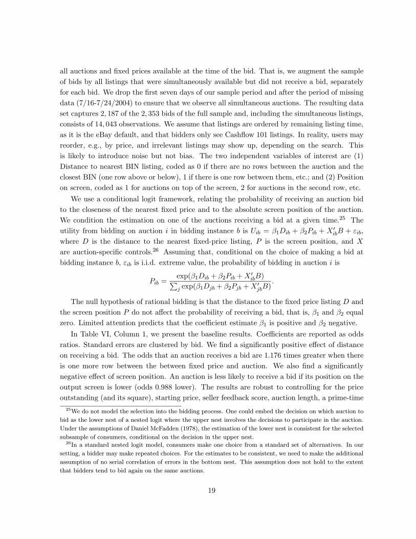
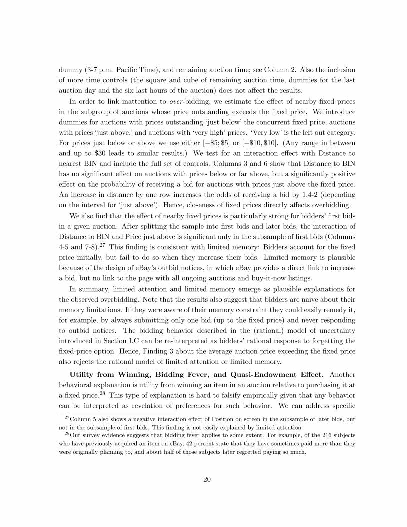

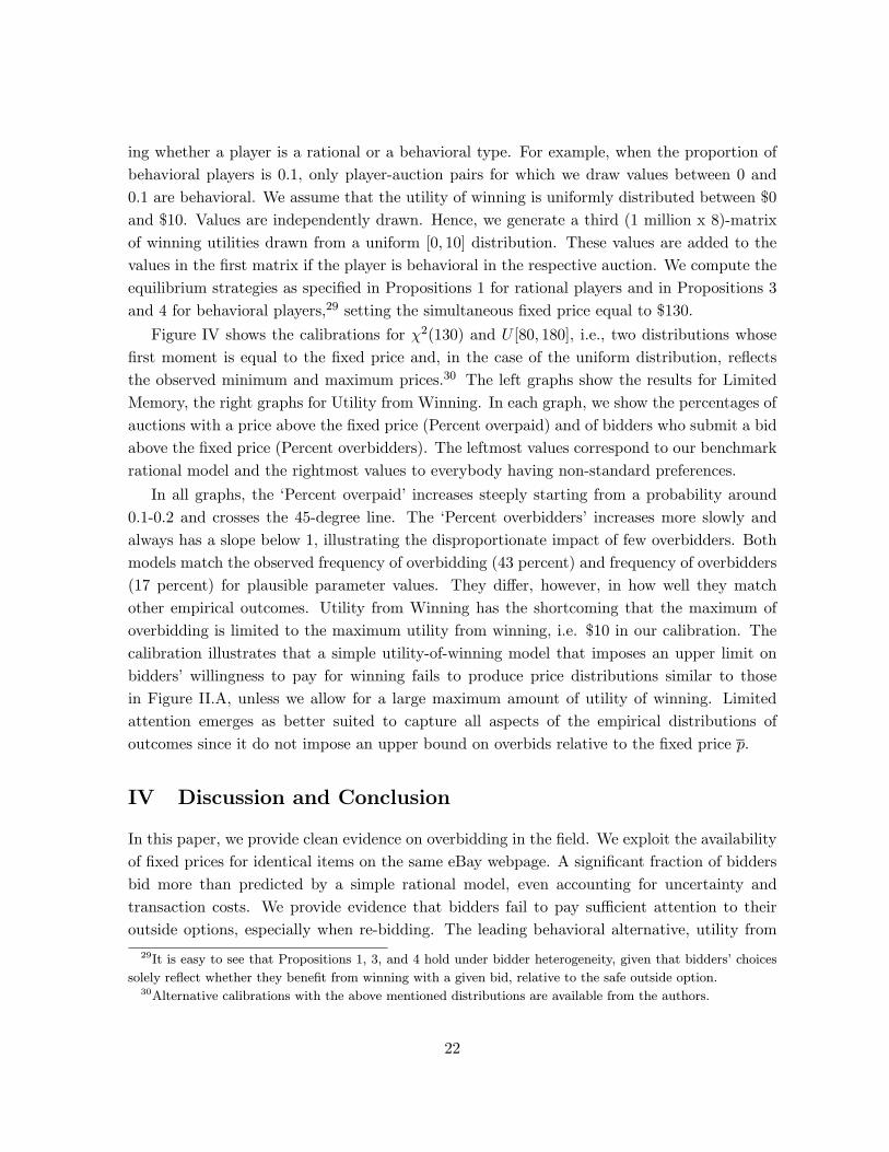


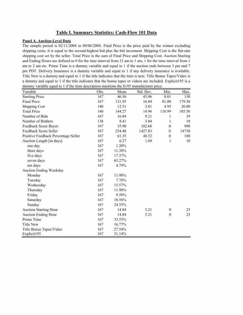
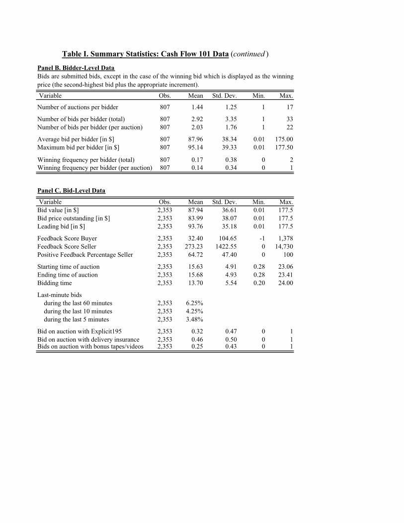
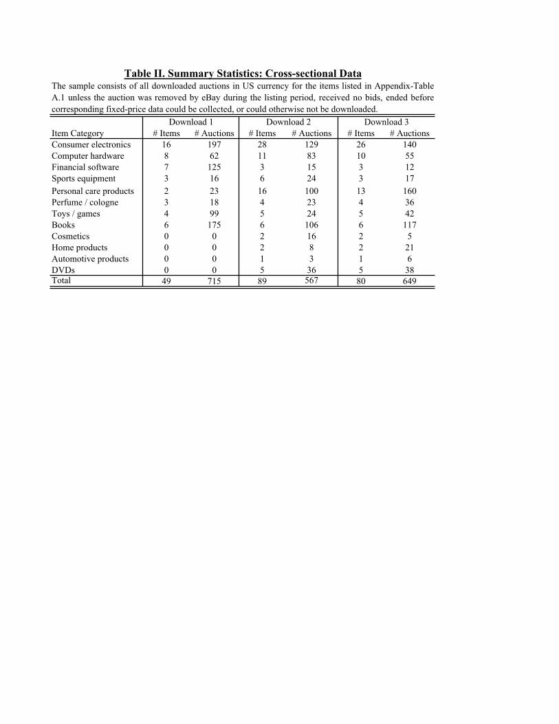
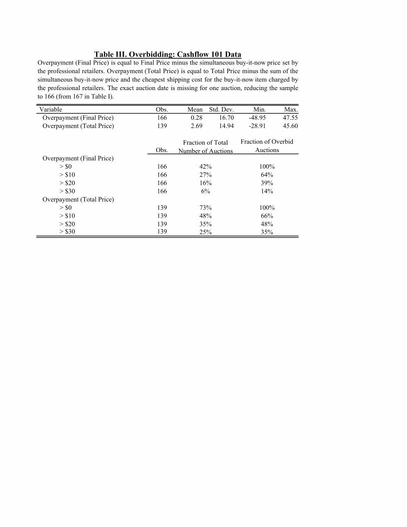
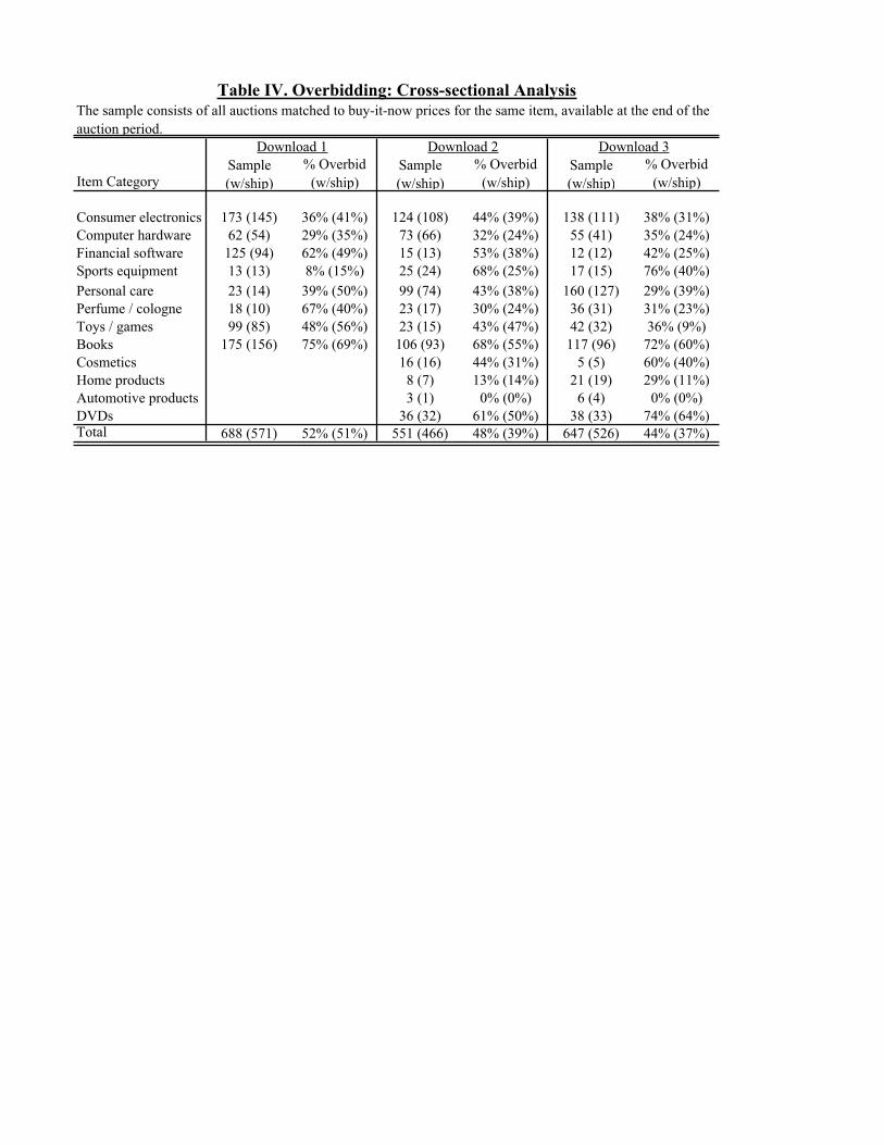


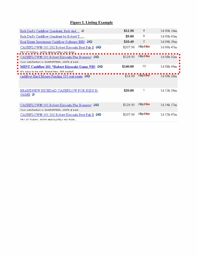


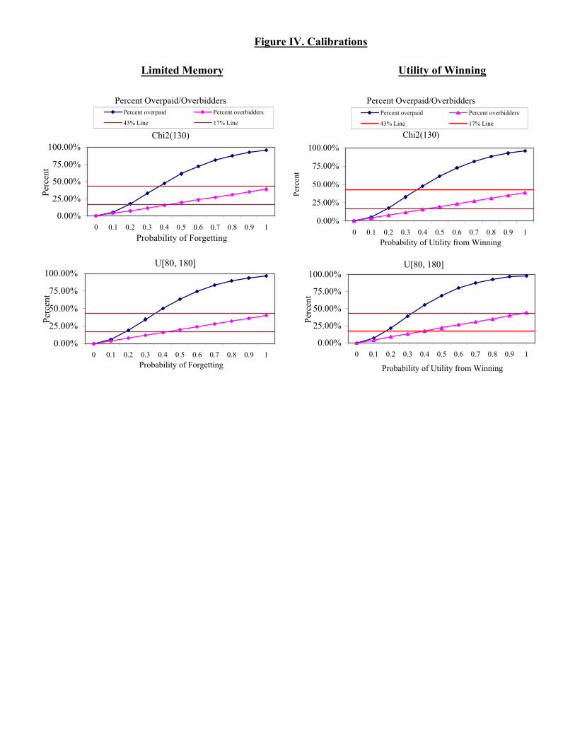


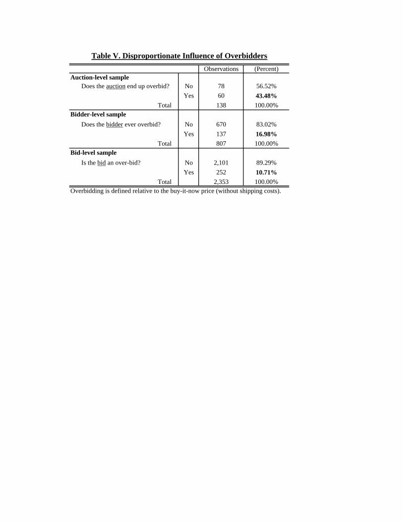

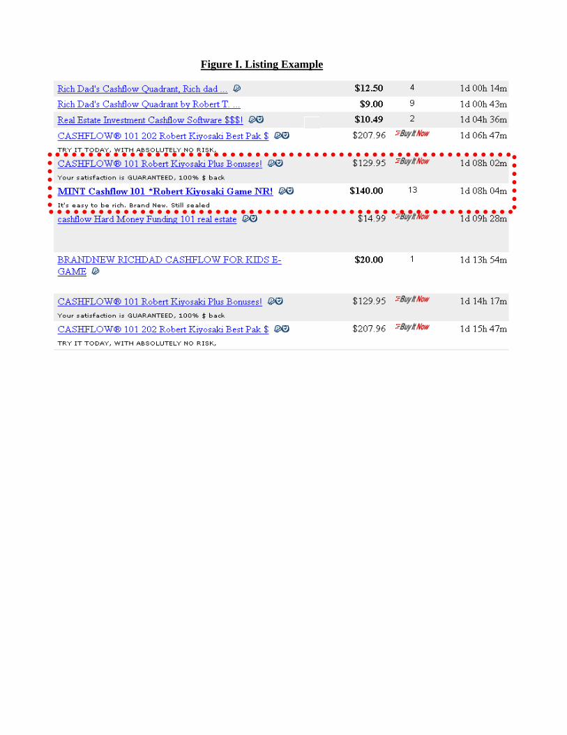
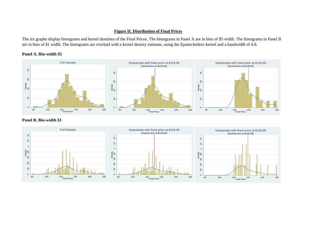


![meinhof, ulrike - bambule [1970].pdf](https://static.documents.pub/doc/80x56/5572010a4979599169a09eb3/meinhof-ulrike-bambule-1970pdf.jpg)


