The bottom-up beta of momentum Pedro Barroso y First version: September 2012 This version: November 2014 Abstract A direct measure of the cyclicality of momentum at a given point in time, its bottom-up beta with respect to the market, forecasts both the returns and the risk of the strategy. Challenging a potential risk-based explanation, a highly cyclical momentum portfolio forecasts both higher risk and lower returns for the strategy. The results show robustness out-of-sample (OOS) and controlling for other variables. One predictive regression of monthly momentum returns on its bottom-up beta produces an OOS R-square of 2.41%. This contrasts with the usual negative OOS R-squares of similar predictive regressions for the market excess return. I thank Alan Gregory, Miguel Ferreira, Pedro Santa-Clara, and Ronald Masulis for their suggestions. y University of New South Wales, School of Banking and Finance. E-mail: [email protected]1
Transcript
The bottom-up beta of momentum∗
Pedro Barroso†
First version: September 2012
This version: November 2014
Abstract
A direct measure of the cyclicality of momentum at a given point in time, its
bottom-up beta with respect to the market, forecasts both the returns and the risk
of the strategy. Challenging a potential risk-based explanation, a highly cyclical
momentum portfolio forecasts both higher risk and lower returns for the strategy.
The results show robustness out-of-sample (OOS) and controlling for other variables.
One predictive regression of monthly momentum returns on its bottom-up beta
produces an OOS R-square of 2.41%. This contrasts with the usual negative OOS
R-squares of similar predictive regressions for the market excess return.
∗I thank Alan Gregory, Miguel Ferreira, Pedro Santa-Clara, and Ronald Masulis for their suggestions.†University of New South Wales, School of Banking and Finance. E-mail: [email protected]
1
1 Introduction
Unconditionally, the Fama-French factors do not explain the risk or the returns of mo-
mentum (Fama and French (1996)). But Grundy and Martin (2001) show this is because
momentum portfolios have time-varying systematic risk and this is not captured in un-
conditional regressions.
The beta of the winners-minus-losers portfolio should depend by construction on the
previous returns of the market. For instance, in late 1999, and after good returns in the
stock market, the winners were mostly high beta stocks while the laggards were low beta
stocks. Hence the momentum portfolio, short on previous losers and long on previous
winners, should have a high beta by design. By contrast, at the end of 2008, in an
extreme bear market, previous losers should be typically stocks with high betas such as
financial firms at the time, while the group of winner stocks would have low betas. Thus
the momentum portfolio would have a negative beta by construction.
I compute the bottom-up beta of momentum using monthly returns from January
1950 to December 2012 for all stocks in the Center of Research for Security Prices
(CRSP). The bottom-up betas change quite substantially over time, ranging from a
minimum of -1.71 to a maximum of 2.09 and are positively related to previous returns
in the market.
Bottom-up betas are much better at explaining the risk of momentum than one
unconditional regression. The bottom-up betas with respect to the Fama-French factors
explain 39.59 percent of the out-of-sample variation in momentum returns, nearly 17
times more than one unconditional regression. They also compare favorably to other
methods of estimation of the conditional beta.
On the other hand, it is known that it is not persistence in returns of the Fama-
French factors that explains momentum profits (Grundy and Martin (2001), Blitz, Huij,
and Martens (2011), Chaves (2012)). As such, large loadings of momentum on some
other factors should constitute a warning against the attractiveness of investing in the
strategy.
The expected return of momentum diminishes significantly with the absolute loading
of the strategy on the market. An increase of one standard deviation in the absolute
value of the market beta leads to a 1.18 percentage points decrease in momentum’s
2
monthly expected return. One regression of momentum returns using this predictive
variable holds an out-of-sample (OOS) R-square of 2.41%, a very high value for a monthly
frequency. This contrasts with the predictability of the market, where similar regressions
typically have negative R-squares (Goyal and Welch (2008)). In fact, the predictive
models that show more robustness for the market achieve OOS R-squares of about 1%
for the same frequency, so the predictability of momentum returns is more than double
that of the market.
The absolute loading of momentum on the market also forecasts its risk. One pre-
dictive regression of the realized variance of momentum on the absolute value of its beta
holds an OOS R-square of 8.25 percentage points.
The results of predictive regressions for risk and returns are robust controlling for
other variables found relevant in the literature. In particular, the absolute loading on
the market is not subsumed by the market being in a bear state (Cooper, Gutierrez, and
Hameed (2004)) and the recent volatility of the market (Wang and Xu (2011); and Tang
and Xu (2012)).
One possible use of time-varying betas is to hedge the systematic risk of momentum
(Grundy and Martin (2001); Daniel and Moskowitz (2011); and Martens and Oord
(2014)). I examine the usefulness of bottom-up betas to hedge the risk of momentum in
real time and find that it does not avoid its large drawdowns. The hedged strategy still
has a high excess kurtosis and a pronounced left-skew, so the crash risk is not removed by
hedging. Daniel and Moskowitz (2011) estimate the beta of momentum with a regression
of daily returns and they also find momentum investors could not use time-varying betas
to avoid the crashes in real time. This contrasts with the benefits of using the time-
varying volatility of momentum to manage its risk (Barroso and Santa-Clara (2014)).
2 The time-varying beta of momentum
The momentum portfolio changes its composition as new stocks join the group of pre-
vious losers or the group of previous winners. This changing composition induces time
variation in the beta of the portfolio with respect to the market. I compare three meth-
ods of estimation of these time-varying betas: i) a bottom-up approach; ii) estimating
beta as a linear function of factor returns in the formation period; iii) a high-frequency
3
beta estimated from daily returns.
The bottom-up beta of the momentum portfolio is the weighted average of individual
betas in the portfolio:
βBU,t =
Nt∑i=1
wi,tβ̂i,t (1)
where Nt is the number of stocks in the portfolio at time t, wi,t is the weight of stock
i in the WML portfolio and β̂i,t is the beta of the individual stock estimated from past
monthly returns. This beta relies only on past information, known before time t, so its
forecasts are out-of-sample (OOS) by construction.1
Figure 1 shows the bottom-up beta of the momentum strategy and compares it with
the unconditional beta, obtained from running a regression of the WML on the market
with the full sample.
The unconditional beta is -0.27. So on average the losers portfolio has a higher beta
than the winners portfolio. But this unconditional beta masks substantial time-variation
in the composition of the WML portfolio. The bottom-up beta ranges from -1.71 to 2.09.
Therefore, the momentum strategy is at times highly exposed to the overall stock market,
while at other times it is actually negatively related with the market.
Grundy and Martin (2001) show that the time-varying systematic risk of momentum
is due to the return of the overall market during the formation period. After bear mar-
kets, winners tend to be low-beta stocks while losers are high-beta stocks. By shorting
losers to go long winners, the WML portfolio will have by construction a negative beta.
The opposite happens after bull markets. Figure 2 illustrates this point, confirming the
results of Grundy and Martin (2001) and Korajczyk and Sadka (2004).
The bottom-up beta, obtained from the individual stock level, is approximately a
linear function of market returns during the formation period. Following Grundy and
Martin (2001), I estimate this beta running an OLS regression:
rwml,t = α+ β0rmrft + β1rmrftrmrft−2,t−12 (2)
where rmrft−2,t−12 is the cumulative excess return of the market during the formation
period of the momentum portfolio. Then the time-varying linear beta is:
1 I describe with more detail the method of estimation of the bottom-up betas in the annex.
4
βL,t = β0 + β1rmrft−2,t−12 (3)
Another method to estimate the time-varying beta of momentum is to use the daily
returns of the WML portfolio and those of the market. Following Daniel and Moskowitz
(2011) we regress at the end of each month the daily returns of momentum on the
market in the previous 126 sessions (≈ 6 months).2 As the bottom-up beta, the one-
month lagged high-frequency beta (βHF,t−1) produces an OOS forecast of momentum’s
exposure to the market.
Table 1 presents descriptive statistics for different estimates of beta. The uncondi-
tional beta is the estimate from on OLS regression, which is constant. The first two
rows show the in-sample results for βunc and βL using returns from 1964:02 to 2010:12.3
The third and fourth rows present the OOS results for the same variables. Here I use
the period from 1950:01 to 1964:01 to obtain initial estimates of the betas, producing
an OOS forecast for the following month. Then I re-iterate the procedure every month
till the end of the sample using an expanding window of monthly observations. The
resulting OOS period is from 1964:02 to 2010:12.
The in-sample (out-of-sample) linear beta varies between a minimum of -1.74 (-
1.60) and a maximum of 1.61 (1.46). The high-frequency beta varies even more from
a minimum of -1.94 to a maximum of 2.16. So all estimates show there is substantial
time-variation in the market exposure of the momentum strategy.
A relevant test is whether time-varying betas explain the risk and returns of momen-
tum. For each estimation method I obtain the hedged momentum return as:
zt = rwml,t − β̂trmrft (4)
where β̂t is the conditional beta at time t.
Table 2 shows that time-varying risk does not explain the excess returns of the
momentum strategy. The mean excess return of the market-hedged momentum strategy
ranges from 1.19 percent per month to 1.47 percent per month. All the t-statistics
2They estimate the beta using 10 lags of daily returns to correct for stale quotes. This correctiondoes not improve results in my sample period, so I only repport results from regressions with no lags.
3To facilitate the comparison, the same sample period is examined for all methods. The daily returnsof the Fama-French factors is only available starting in 1963:07. This restricts the comparable sampleperiod to start in 1964:02.
5
exceed four, so they are highly significant. This confirms the results of Grundy and
Martin (2001) and Blitz, Huij, and Martens (2011). Grundy and Martin (2001) show
that time-varying risk does not explain the alpha of momentum. Conversely, Blitz,
Huij, and Martens (2011) and Chaves (2012) show that momentum profits come from
persistence in returns at the individual stock level, rather than in the factors themselves.
As a result, hedging market risk has little effect on the alpha of momentum.
Momentum has more beta risk in ‘good times’(in bull markets) than in ‘bad times’
(in bear markets). The opposite pattern should hold for time-varying beta to explain
momentum average excess returns.
But taking time-varying betas into consideration enhances substantially the under-
standing of momentum’s risk. The R-squared (1 − var(zt)var(rwml,t)
) improves OOS from just
1.93 percent for the unconditional model to values ranging from 15.78 percent to 24.81
percent using the conditional models.4 This is 8 to nearly 13 times more than the uncon-
ditional model. The bottom-up beta performs particularly well OOS, with the highest
R-square among those considered.
3 Exposure to the Fama-French factors
One unconditional OLS regression of monthly momentum returns on the Fama-French
factors from 1964:02 to 2010:12 holds (t-statistics in parenthesis):
The regression has an adjusted R-square of just 5.63 percent and a significant positive
alpha of 1.71 percent, confirming the result in Fama and French (1996) that their factors
do not explain the risk and returns of momentum. Still, this improves substantially the
fit of the CAPM, which has an adjusted R-square of just 2.54 percent for the same period.
This is mainly because momentum is significantly and negatively related to value. Yet,
as for the exposure to the market, these estimates mask substantial time-variation in
risk.4Note that the OOS r-squared can assume negative values. Goyal and Welch (2008) show this is often
the case with predictive regressions.
6
Figure 3 shows the exposure of momentum to the market (RMRF), value (HML),
and size (SMB) factors. Just as for the market, exposure to value and size varies a lot.5
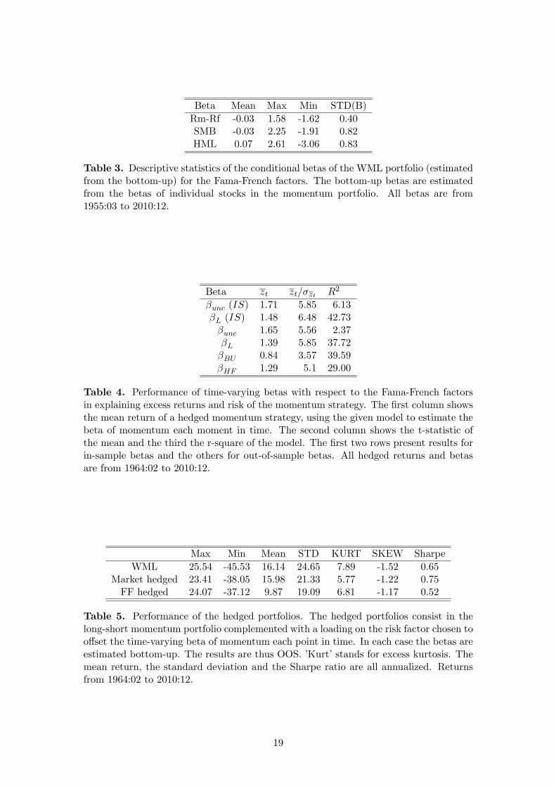
Table 3 shows the descriptive statistics of the bottom-up betas. The exposure of
the momentum portfolio to size and value varies even more than the exposure to the
market. For the HML factor, the beta ranges from -3.06 to 2.61, while for the market it
ranges only from -1.62 to 1.58. The standard deviation of the betas with respect to size
and value are, respectively, 0.82 and 0.83. This is more than the standard deviation of
βrmrf .
Table 4 shows the average excess returns of the hedged portfolio with respect to the
Fama-French factors, its t-statistics and R-square.
As for the CAPM, the conditional models do not explain the mean excess returns
of momentum which have always a positive mean with significant t-statistics ranging
between 3.57 (for the bottom-up beta) and 6.48 (for the beta linear with past returns).
However, the conditional models improve considerably the understanding of the sys-
tematic risk of momentum. In sample, the R-square of the unconditional model is 6.13
percent, which is reduced to only 2.37 percent in the out-of-sample (OOS) test. The
high-frequency beta, used in Daniel and Moskowitz (2011), produces an OOS R-square
of 29 percent. In spite of this large improvement, the high frequency approach underper-
forms other measures of systematic risk. The linear model has an OOS R-square of 37.72
percent. Even more so, bottom-up betas explain 39.59 percent of the systematic risk of
momentum OOS. This is nearly 17 times more than the unconditional model. As for
the CAPM, the bottom-up beta is the best conditional model to explain the systematic
risk of momentum.
4 Predicting the risk and return of momentum
At times, the momentum portfolio is well characterized by a directional exposure on
the persistence of returns for some factor. The bottom-up betas constitute a direct and
real-time measure of this. But the source of momentum returns is more likely to be
persistence in returns at the stock level, not in factor returns. As such, a larger beta (in
absolute value) should forecast a lower return for the momentum portfolio.
5 In unreported results, I find that the betas w.r.t. to each factor are positively related. Yet most oftheir variation is idiosyncratic (more than 90 percent). They do not move in tandem with each other.
7
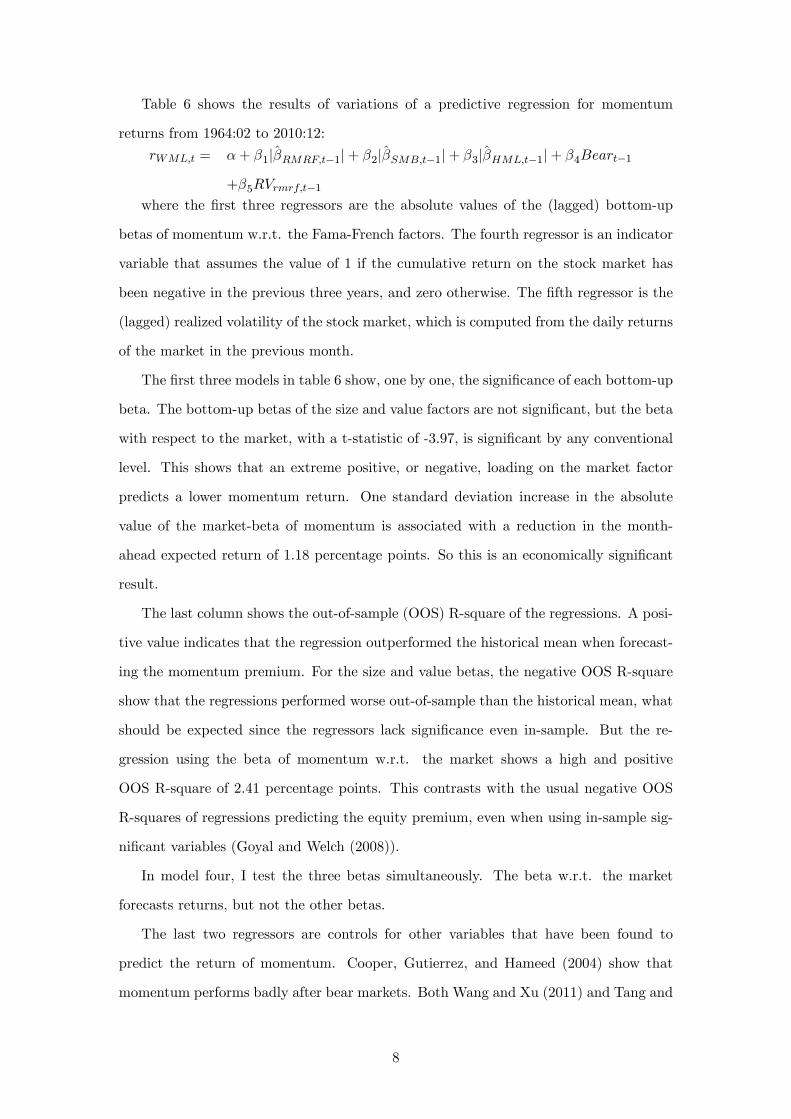
Table 6 shows the results of variations of a predictive regression for momentum
+β5RVrmrf,t−1where the first three regressors are the absolute values of the (lagged) bottom-up
betas of momentum w.r.t. the Fama-French factors. The fourth regressor is an indicator
variable that assumes the value of 1 if the cumulative return on the stock market has
been negative in the previous three years, and zero otherwise. The fifth regressor is the
(lagged) realized volatility of the stock market, which is computed from the daily returns
of the market in the previous month.
The first three models in table 6 show, one by one, the significance of each bottom-up
beta. The bottom-up betas of the size and value factors are not significant, but the beta
with respect to the market, with a t-statistic of -3.97, is significant by any conventional
level. This shows that an extreme positive, or negative, loading on the market factor
predicts a lower momentum return. One standard deviation increase in the absolute
value of the market-beta of momentum is associated with a reduction in the month-
ahead expected return of 1.18 percentage points. So this is an economically significant
result.
The last column shows the out-of-sample (OOS) R-square of the regressions. A posi-
tive value indicates that the regression outperformed the historical mean when forecast-
ing the momentum premium. For the size and value betas, the negative OOS R-square
show that the regressions performed worse out-of-sample than the historical mean, what
should be expected since the regressors lack significance even in-sample. But the re-
gression using the beta of momentum w.r.t. the market shows a high and positive
OOS R-square of 2.41 percentage points. This contrasts with the usual negative OOS
R-squares of regressions predicting the equity premium, even when using in-sample sig-
nificant variables (Goyal and Welch (2008)).
In model four, I test the three betas simultaneously. The beta w.r.t. the market
forecasts returns, but not the other betas.
The last two regressors are controls for other variables that have been found to
predict the return of momentum. Cooper, Gutierrez, and Hameed (2004) show that
momentum performs badly after bear markets. Both Wang and Xu (2011) and Tang and
8
Xu (2012) show that momentum has lower returns in volatile markets. Testing all these
simultaneously shows that the market-beta of momentum is significant controlling for the
other variables. This regression is not robust OOS as using too many regressors increases
the chances for in-sample overfitting, even if some predictors are indeed significant.
Daniel and Moskowtiz (2011) find that momentum crashes are due to the option-like
payoffs of the losers portfolios in extreme bear markets. As the bottom-up market beta
of momentum tends to be very negative in those situations, it is pertinent to examine if
my results are not driven by negative betas and momentum crashes alone. To test for
this, the following OLS regression distinguishes between positive and negative bottom-up
betas. It holds (t-statistics in parenthesis):
rWML,t = 2.56 −3.46 β̂+
RMRF,t−1 +4.70 β̂−RMRF,t−1
(6.05) (−2.71) (3.75)
where β̂+
RMRF,t−1 is the value of the beta of momentum w.r.t. the market if positive
and β̂−RMRF,t−1 the same if negative.
The results are stronger for the left tail of the bottom-up beta. A marginal increase
in the negative beta reduces the expected return of momentum more than in a positive
beta. But the predictability is quite significant in the right tail as well. A high positive
beta predicts lower returns for momentum, with a t-statistic of -2.71, the variable is
significant at the 1% level. So the result is not driven by the negative betas, momentum
crashes and option-like payoffs alone.6
As there is a large momentum crash in the sample, I also test for non-linearities in
this relation running a step-wise regression:
rWML,t = 2.64 −5.18 |β̂m−,t−1| −3.17 |β̂m+,t−1|
(6.19) (−4.00) (−2.55)where |β̂m−,t−1| is the absolute value of the bottom-up beta w.r.t. the market if this
value is below the median and |β̂m+,t−1| the same if it is above the median. I find the
results are not totally driven by observations with particularly high absolute values of
beta w.r.t the market. In fact, there is a slightly stronger association for smaller absolute
values of the predictor variable.
Another important issue is whether the bottom-up betas of momentum help predict
its risk. Table 7 presents variations of the predictive regression:
6 In fact, in unreported results, I find there is no supportive evidence that the market-beta of momen-tum forecasts market reversals, which have been interpreted as the cause of momentum crashes.
+β5RVrmrf,t−1 + β6RVwml,t−1where the dependent variable is the realized variance of momentum, at a monthly
frequency. The regressors are the same as above for predicting returns, except for the
last one which is the lagged value of momentum’s realized variance. Barroso and Santa-
Clara (2014) show the risk of momentum is highly predictable using its own lagged value
as a predictor. As such it is important to control for this variable.
The first three regressions show that the betas w.r.t. the market and value factors
are significant, but the beta of the size factor is not. The regressions that use the value
and market betas are robust, with an OOS R-square as high as 8.25 percentage points for
the market. The fourth regression includes all three variables and confirms this result.
The fifth regression includes the two control variables (the lagged risk of the market
and the state of the market). The bottom-up betas of the market and value factors
remain significant. The last model includes the lagged realized variance of momentum.
This variable with a t-statistic of 21.88 is highly significant and it increases the OOS
R-square from 22.77 percentage points to 53.84 percentage points. The significance of
the bottom-up beta of momentum w.r.t. the market remains significant but the beta
w.r.t. the value factor does not.
In general, the predictability of momentum’s risk is much higher than the predictabil-
ity of its returns. The most relevant predictor is the lagged value of momentum’s risk.
Still, the bottom-up beta of momentum w.r.t the market is significant in every regres-
sion considered and robust OOS. So a highly cyclical (or counter-cyclical) momentum
portfolio predicts a higher risk going forward.
5 Systematic risk and momentum crashes
Grundy and Martin (2001) find that hedging the time-varying risk exposures of mo-
mentum produces stable returns. Daniel and Moskowitz (2011) show that this relies on
using ex post information and that hedging in real time with time-varying betas does
not avoid the momentum crashes. However, their method of estimating the time varying
risk is with top-down regressions of daily data —the high-frequency beta. I find this is
a less satisfactory approach to capture the time-varying systematic risk of momentum
10
(although it still clearly outperforms an unconditional model).
Bottom-up betas provide a superior method to estimate the time-varying exposure
of momentum to other factors. This leads to the question of whether hedging this time-
varying risk with a more suitable method could avoid the large drawdowns of momentum.
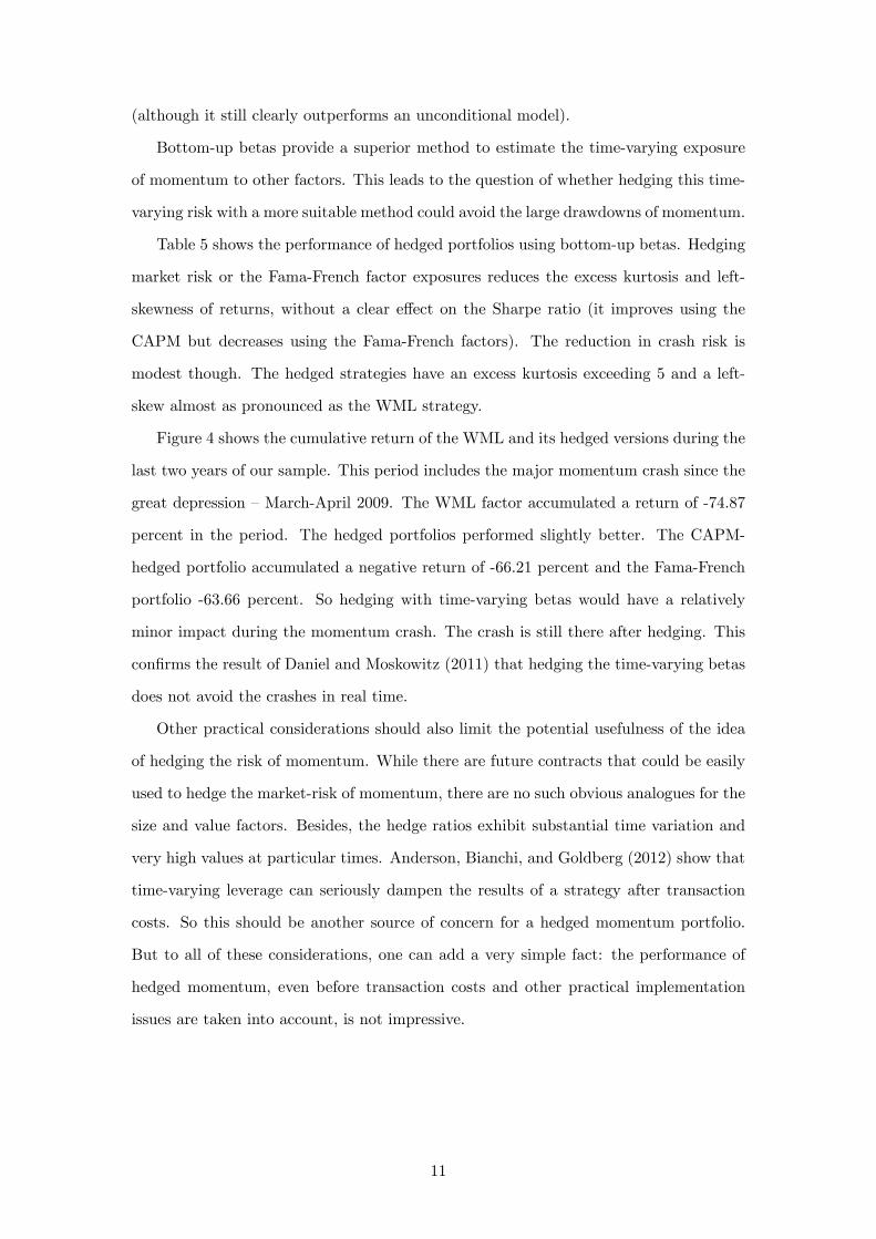
Table 5 shows the performance of hedged portfolios using bottom-up betas. Hedging
market risk or the Fama-French factor exposures reduces the excess kurtosis and left-
skewness of returns, without a clear effect on the Sharpe ratio (it improves using the
CAPM but decreases using the Fama-French factors). The reduction in crash risk is
modest though. The hedged strategies have an excess kurtosis exceeding 5 and a left-
skew almost as pronounced as the WML strategy.
Figure 4 shows the cumulative return of the WML and its hedged versions during the
last two years of our sample. This period includes the major momentum crash since the
great depression —March-April 2009. The WML factor accumulated a return of -74.87
percent in the period. The hedged portfolios performed slightly better. The CAPM-
hedged portfolio accumulated a negative return of -66.21 percent and the Fama-French
portfolio -63.66 percent. So hedging with time-varying betas would have a relatively
minor impact during the momentum crash. The crash is still there after hedging. This
confirms the result of Daniel and Moskowitz (2011) that hedging the time-varying betas
does not avoid the crashes in real time.
Other practical considerations should also limit the potential usefulness of the idea
of hedging the risk of momentum. While there are future contracts that could be easily
used to hedge the market-risk of momentum, there are no such obvious analogues for the
size and value factors. Besides, the hedge ratios exhibit substantial time variation and
very high values at particular times. Anderson, Bianchi, and Goldberg (2012) show that
time-varying leverage can seriously dampen the results of a strategy after transaction
costs. So this should be another source of concern for a hedged momentum portfolio.
But to all of these considerations, one can add a very simple fact: the performance of
hedged momentum, even before transaction costs and other practical implementation
issues are taken into account, is not impressive.
11
6 Conclusion
When the previous returns of a factor are high, the momentum portfolio rotates from
low-beta stocks to high-beta stocks on that factor. This changes the betas of momentum
over time.
Conditional betas capture the systematic risk of momentum much better than an
unconditional model. Using the Fama-French factors, the out-of-sample R-square in-
creases from just 2.37 percent for the unconditional model to as much as 39.59 percent
using conditional betas.
The bottom-up betas perform particularly well in capturing time variation in system-
atic risk. They achieve the best results comparing to the linear and the high-frequency
beta, both with the CAPM and the Fama-French factors. Using this method to hedge
the time-varying betas of momentum does not avoid its crashes though or translate into
any significant improvement.
Conventional momentum is a less appealing strategy whenever it relies excessively on
a (positive or negative) loading in the market factor. This forecasts both lower returns
and higher risk for the strategy.
This happens because the stocks in both legs of the portfolio are most likely selected
on the basis of their high exposure to the market in the formation window. The market
may have performed very well, or very badly, in that period but that says very little
about its performance going forward. On the other hand, it does convey important
information about the future performance of momentum.
12
Annex
To estimate the bottom-up betas, I use data from CRSP (Center for Research in Security
Prices) with monthly returns for all stocks listed in the NYSE, AMEX or NASDAQ
from January 1950 to December 2010. Following the standard practice, the momentum
portfolios are sorted according to accumulated returns in the formation period which is
from month t-12 to month t − 2. The stocks are classified into deciles using as cutoff
points the universe of all firms listed on the NYSE. This way there is an equal number
of firms listed in the NYSE in each decile. This is to prevent the possibility of very small
firms dominating either the long or short leg of the portfolio.
In order to be considered in the portfolio a firm’s stock must have a valid return in
month t−2, a valid price in month t−13, and information on the market capitalization of
the firm in the previous month. We take into consideration the delisting return of a stock
whenever it is available. Individual stocks are value-weighted within each decile. The
return of the winner-minus-losers (WML) is simply the return of the top decile portfolio,
sorted on previous momentum, minus the return of the bottom decile portfolio.
I estimate the beta of each individual stock running an OLS regression of its monthly
excess return on the excess return of the market from t − 61 to t − 2, the end of the
formation period. I require at least 24 valid returns in that period to estimate the beta.
The market return is the value-weighted return of all stocks in the CRSP universe, as
obtained from Kenneth French’s online data library.
13
References
[1] Anderson, R., S. Bianchi, and L. Goldberg (2012). “Will My Risk Parity Strategy
Outperform?”, Financial Analysts Journal, 68(6), pp. 75-93.
[2] Barroso, P. and P. Santa-Clara (2014). “Momentum has its moments”, forthcoming
in the Journal of Financial Economics.
[3] Blitz, D., J. Huij, and M. Martens (2011). “Residual momentum”, Journal of Em-
pirical Finance, Vol 18, 3. pp. 506-521.
[4] Chaves, D. (2012). “Eureka! A momentum strategy that also works in Japan”,
working paper.
[5] Cooper, M., R. Gutierrez Jr., and A. Hameed (2004). “Market states and momen-
tum”, The Journal of Finance, 59 (3), pp. 1345-1366.
[6] Daniel, K., and T. Moskowitz (2011).“Momentum crashes”, Working paper.
[7] Fama, E. and K. French (1992). “The cross-section of expected stock returns”, The
Journal of Finance, vol. 47, no. 2, pp. 427-465.
[8] Fama, E. and K. French (1996). “Multifactor explanations of asset pricing anom-
alies”, The Journal of Finance, vol. 51, no. 1, pp. 55-84.
[9] Goyal, A., and I. Welch (2008). “A comprehensive look at the empirical performance
of equity premium prediction”, Review of Financial Studies 21, pp. 1455-1508.
[10] Grundy, B., and J. S. Martin (2001). “Understanding the nature of the risks and
the source of the rewards to momentum investing”, Review of Financial Studies,
14, pp. 29-78.
[11] Jegadeesh, N., and S. Titman (1993). “Returns to buying winners and selling losers:
Implications for stock market effi ciency”, The Journal of Finance, vol. 48, no. 1, pp.
65-91.
[12] Martens, M., and A. Oord (2014). “Hedging the time-varying risk exposures of
momentum returns”, Journal of Empirical Finance, vol. 28, pp. 78-89.
[13] Tang, F., and J. Mu (2012). “Market Volatility and Momentum”, working paper.
14
[14] Wang, K., and W. Xu (2011). “Market Volatility and Momentum”, working paper.
15
Tables and Figures
60 65 70 75 80 85 90 95 00 05 10
1.5
1
0.5
0
0.5
1
1.5
2
Market beta of WML portfolioBe
ta o
f WM
L po
rtfol
io
Time
βbu
βunc
Figure 1. Bottom-up and unconditional beta of the WML portfolio. The bottom-upbeta of the WML portfolio is obtained from the previous 5 years of monthly returns ofindividual stocks. Returns from 1955:03 to 2010:12.
16
0.4 0.6 0.8 1 1.2 1.4 1.6 1.82
1.5
1
0.5
0
0.5
1
1.5
2
2.5Market beta of WML and return in the formation period
Beta
of W
ML
portf
olio
Gross return on market portfolio from t12 to t2
β t
β t = 2.76 + 2.55 rmrft2,t12
Figure 2. The bottom-up beta of the WML portfolio w.r.t. the market and the previousone-year return on the market portfolio. All returns from 1955:03 to 2010:12.
Table 1. Descriptive statistics of different betas of momentum. The first is the betafrom one unconditional regression of the returns of the WML portfolio on the market.The second is a conditional regression where the beta depends linearly on the previousone-year return of the market. The third and fourth rows present the results for thesesame regressions but out-of-sample. The fifth row shows the results for the bottom-upbeta of momentum w.r.t. the market. The final row shows the results for the high-frequency beta estimated from daily returns of momentum in the previous 6 months.The bottom-up and high-frequency betas are out-of-sample. All betas are from 1964:02to 2010:12. The final column shows the standard deviation of the beta estimate.
Table 2. Performance of time-varying betas in explaining the excess returns and riskof the momentum strategy. The first column shows the average return of a hedgedmomentum strategy using the estimated betas as hedge ratios. The second columnshows the t-statistic of the mean return of the hedged momentum strategy. The finalcolumn shows the r-squared of the model for the risk of momentum. The first two rowspresent results for in-sample betas and the others for out-of-sample betas. All hedgedreturns and betas are from 1964:02 to 2010:12.
1960 1970 1980 1990 2000 2010
1
0
1
Bet
a
Load on RmRf
1960 1970 1980 1990 2000 2010
1
0
1
2
Bet
a
Load on SMB
1960 1970 1980 1990 2000 2010
2
0
2
Bet
a
Load on HML
Figure 3. The loading of the WML on the FF factors using bottom-up betas. Thebottom-up betas are estimated from the betas of individual stocks in the momentumportfolio. The sample period is from 1955:02 to 2010:02.
18
Beta Mean Max Min STD(B)Rm-Rf -0.03 1.58 -1.62 0.40SMB -0.03 2.25 -1.91 0.82HML 0.07 2.61 -3.06 0.83
Table 3. Descriptive statistics of the conditional betas of the WML portfolio (estimatedfrom the bottom-up) for the Fama-French factors. The bottom-up betas are estimatedfrom the betas of individual stocks in the momentum portfolio. All betas are from1955:03 to 2010:12.
Table 4. Performance of time-varying betas with respect to the Fama-French factorsin explaining excess returns and risk of the momentum strategy. The first column showsthe mean return of a hedged momentum strategy, using the given model to estimate thebeta of momentum each moment in time. The second column shows the t-statistic ofthe mean and the third the r-square of the model. The first two rows present results forin-sample betas and the others for out-of-sample betas. All hedged returns and betasare from 1964:02 to 2010:12.
Max Min Mean STD KURT SKEW SharpeWML 25.54 -45.53 16.14 24.65 7.89 -1.52 0.65
Table 5. Performance of the hedged portfolios. The hedged portfolios consist in thelong-short momentum portfolio complemented with a loading on the risk factor chosen tooffset the time-varying beta of momentum each point in time. In each case the betas areestimated bottom-up. The results are thus OOS. ’Kurt’stands for excess kurtosis. Themean return, the standard deviation and the Sharpe ratio are all annualized. Returnsfrom 1964:02 to 2010:12.
19
0 5 10 15 20 250.2
0.3
0.4
0.5
0.6
0.7
0.8
0.9
1
1.1
1.2
cum
ulat
ive
retu
rn
WMLCAPMhedgedFFhedged
Figure 4. Momentum crash. The cumulative returns of the WML portfolio (blue), themomentum portfolio hedged for market risk (green) and for the Fama-French factors(red). Returns from 2008:12 to 2010:12.
20
Model Const RMRF SMB HML Bear RVrmrf adj-R2 OOS R2
Table 6. Predictive regressions of the return of the WML portfolio on the absolutevalue of the bottom up-betas of momentum with respect to the Fama-French factors.In model 5, we include the bear market indicator function and the lagged one-monthrealized variance of the market. The bear market indicator assumes the value of 1 ifthe cumulative return of the market for the previous 3 years is negative. The returnsare from 1964:02 to 2010:12. The coeffi cients are multiplied by 100 for readability. Itst-statistics are in squares brackets. The R-squares are in percentage points. The lastcolumn shows the out-of-sample r-squared, this is computed using an expanding windowof observations after an initial in-sample period of 240 months.
Table 7. Predictive regressions of the monthly realized variance of the WML portfolio onthe absolute value of the bottom-up betas of momentum with respect to the Fama-Frenchfactors. In model 5, we include the bear market indicator function, the lagged one-monthrealized variance of the market and the lagged one-month realized variance of momentumitself. The bear market indicator assumes the value of 1 if the cumulative return of themarket for the previous 3 years is negative. The forecasted realized variances are from1964:02 to 2010:12. The coeffi cients are multiplied by 100 for readability, its t-statisticsare in squares brackets. The R-squares are in percentage points. The returns are from1964:02 to 2010:12. The coeffi cients are multiplied by 100 for readability. Its t-statisticsare in squares brackets. The R-squares are in percentage points. The last column showsthe out-of-sample r-squared, this is computed using an expanding window of observationsafter an initial in-sample period of 240 months.