Bachelor Thesis The Boundary Layer over a Flat Plate July 4, 2014 M.P.J. Sanders Faculty of Engineering Technology Engineering Fluid Dynamics Examination committee: Prof.dr.ir. H.W.M. Hoeijmakers (Mentor/Chairman) Dr. H.K. Hemmes (External Member) Ir. R. Kommer (Mentor)
Transcript
Bachelor Thesis
The Boundary Layer over a Flat Plate
July 4, 2014
M.P.J. Sanders
Faculty of Engineering TechnologyEngineering Fluid Dynamics
Examination committee:Prof.dr.ir. H.W.M. Hoeijmakers (Mentor/Chairman)Dr. H.K. Hemmes (External Member)Ir. R. Kommer (Mentor)
i
I Abstract
The properties of the boundary-layer over a flat plate have been investigated analytically, experi-mentally and numerically employing XFOIL. With the theory from Blasius and von Karman, theboundary-layer properties over an infinitesimally thin flat plate have been investigated analytically. Afinite thickness plate, designed to behave aerodynamically as a flat plate, with a Hermite polynomialleading edge and a trailing edge corresponding to the last 70% of a NACA 4-series airfoil section, hasbeen analyzed with XFOIL and has been investigated mounted at zero angle of attack in the SilentWind Tunnel of the University of Twente.
Initial measurements have been performed to obtain the drag force and velocity profile. The dragforce was measured with load cells and the velocity profile was determined with a Pitot tube anda single-wire Hot Wire probe (55P11) at various Reynolds numbers. The measurements indicate adelayed transition from laminar to turbulent flow at a Reynolds number around Recrit=3·106 insteadof the expected Recrit=5·105. Leading-edge turbulence strips were also applied in order to investigatethe drag force and the transitional boundary layer.
The found delayed transition is unfavourable for further research on the influence of the surfaceroughness on transition because of the maximum velocity achievable in the Silent Wind Tunnel. Sincethe turbulence level of the Silent Wind Tunnel is relatively low (approximately 0.25%), other possibil-ities have been investigated on the cause of the delayed transition. Results of numerical simulationsusing XFOIL indicated that a small change in the streamwise pressure gradient can delay transitionsubstantially. Therefore, additional measurements have been performed on the streamwise pressuregradient in the Silent Wind Tunnel. These results indicate an existing streamwise pressure gradientin the test section of the Silent Wind Tunnel which is amplified when the plate is installed in the windtunnel and may have been the cause of the delayed transition.
ii
iii
II Nomenclature
English Symbols
ccdcfcpCfDFgmMNpp∞RecRexStiTuuujU∞vVV∞
m----NNm/s2
kgkg m/s-N/mN/m--m2
N/m%m/sm/sm/sm/sm3
m/s
Length of the plateThe drag coefficientLocal skin friction coefficientThe pressure coefficientTotal skin friction coefficientThe total drag forceForceGravitational accelerationMassMomentumThe amplification factorPressureFree stream pressureReynolds number of the entire plateLocal Reynolds numberSurface areaStress vectorTurbulence levelVelocity in the x-directionVelocity vectorFree stream velocity in the x-directionVelocity in the y-directionVolumeFree stream velocity in the y-direction
Greek Symbols
δδ∗
ηθµνρρ∞σijτ
mm-mkg/msm2/skg/m3
kg/m3
N/mN/m
Boundary layer thicknessDisplacement thicknessDimensionless parameterMomentum ThicknessViscosityKinematic viscosityDensityDensity in the free streamStress tensorShear stress
In 1908, H. Blasius, a student of Prandtl, published a paper about ’The Boundary Layers in Fluidswith Small Friction’. The paper discusses among other things, the two dimensional flow over a flatplate. The boundary-layer equations that Blasius derived were much simpler than the Navier-Stokesequations. Blasius found that these boundary layer equations in certain cases can be reduced to asingle ordinary differential equation for a similarity solution, which we now call the Blasius equation.This same method will be used in this report to derive the boundary layer equations over an infinites-imally thin flat plate. In 1921, von Karman, a former student of Prandtl, developed another form ofthe boundary-layer equations which will also be shown in this report. We will start with the derivationof the continuity equation and Navier-Stokes equation to eventually be able to obtain Blasius’ equation.
With the theory from Blasius and von Karman we will analyse the properties of the boundary layerabove an infinitesimally thin flat plate in two dimensional, steady and incompressible flow. More-over, the drag force exerted on the plate will be measured as well as the velocity profile for differentReynolds numbers. Analytical results will be compared to data obtained from measurements. Themeasurements will be performed in the Silent Wind Tunnel of the University of Twente. Numericalsimulations with XFOIL have also been used to simulate the flow over the designed plate to comparethe validity of the derived theory and to investigate if the designed plate behaves aerodynamically asa flat plate with infinitesimally thickness.
The obtained results will give further insight in the basic principles of the flow over streamlinedbodies. If we can successfully describe the flow over a simple geometry such as the flat plate, it be-comes easier to describe the flow over more complicated geometries using the approximations madefor the basic case of the flow over a flat plate.
1
2
2 Assumptions
Before we derive all the mathematical models, The assumptions that are made to analyse the incom-pressible, steady flow over an infinitesimally thin flat plate are listed.
1. 2-dimensional flow, ∂∂z = 0, i = 1,2
2. Steady flow, ∂∂t=0
3. Incompressible flow, ρ=constant
4. Neglect effects due to gravity ~g = ~0, and other body forces
5. Fourier’s law for heat conduction qi = −k ∂T∂xi6. The physical properties µ, cp, k are constant
7. There are no heat sources
8. Newtonian fluid
9. The tension vector ~t by medium A on B: ti = σijnj
10. The stress tensor: σij = −pδij + τij
11. For a Newtonian fluid the viscous stress tensor is τij = µ(∂ui∂xj
+∂uj∂xi
)+ λδij
∂uk∂xk
12. Stokes: 2µ+ 3λ = 0
Figure 2.1: The two dimensional flat plate analysis
3
4
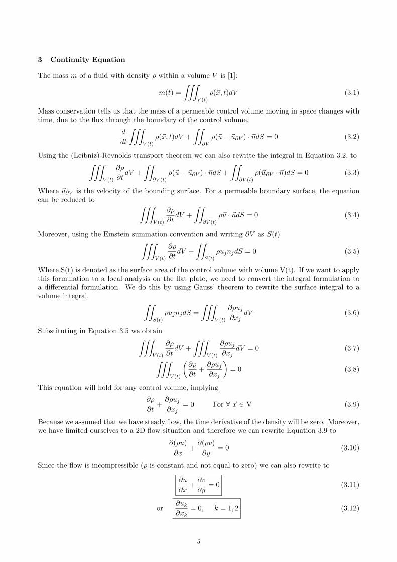
3 Continuity Equation
The mass m of a fluid with density ρ within a volume V is [1]:
m(t) =
∫∫∫V (t)
ρ(~x, t)dV (3.1)
Mass conservation tells us that the mass of a permeable control volume moving in space changes withtime, due to the flux through the boundary of the control volume.
d
dt
∫∫∫V (t)
ρ(~x, t)dV +
∫∫∂Vρ(~u− ~u∂V ) · ~ndS = 0 (3.2)
Using the (Leibniz)-Reynolds transport theorem we can also rewrite the integral in Equation 3.2, to∫∫∫V (t)
∂ρ
∂tdV +
∫∫∂V (t)
ρ(~u− ~u∂V ) · ~ndS +
∫∫∂V (t)
ρ(~u∂V · ~n)dS = 0 (3.3)
Where ~u∂V is the velocity of the bounding surface. For a permeable boundary surface, the equationcan be reduced to ∫∫∫
V (t)
∂ρ
∂tdV +
∫∫∂V (t)
ρ~u · ~ndS = 0 (3.4)
Moreover, using the Einstein summation convention and writing ∂V as S(t)∫∫∫V (t)
∂ρ
∂tdV +
∫∫S(t)
ρujnjdS = 0 (3.5)
Where S(t) is denoted as the surface area of the control volume with volume V(t). If we want to applythis formulation to a local analysis on the flat plate, we need to convert the integral formulation toa differential formulation. We do this by using Gauss’ theorem to rewrite the surface integral to avolume integral. ∫∫
S(t)ρujnjdS =
∫∫∫V (t)
∂ρuj∂xj
dV (3.6)
Substituting in Equation 3.5 we obtain∫∫∫V (t)
∂ρ
∂tdV +
∫∫∫V (t)
∂ρuj∂xj
dV = 0 (3.7)∫∫∫V (t)
(∂ρ
∂t+∂ρuj∂xj
)= 0 (3.8)
This equation will hold for any control volume, implying
∂ρ
∂t+∂ρuj∂xj
= 0 For ∀ ~x ∈ V (3.9)
Because we assumed that we have steady flow, the time derivative of the density will be zero. Moreover,we have limited ourselves to a 2D flow situation and therefore we can rewrite Equation 3.9 to
∂(ρu)
∂x+∂(ρv)
∂y= 0 (3.10)
Since the flow is incompressible (ρ is constant and not equal to zero) we can also rewrite to
∂u
∂x+∂v
∂y= 0 (3.11)
or∂uk∂xk
= 0, k = 1, 2 (3.12)
5
6
4 Navier-Stokes Equation
Newton’s second law states that the rate of change of momentum of an arbitrary control volume offluid is equal to the forces acting on it [1]. We can define the momentum inside the control volume(Equation 4.1) and momentum conservation (Equation 4.2,4.3) as
M(t) =
∫∫∫V (t)
ρ(x, t)u(x, t)dV (4.1)
dM
dt=
d
dt
∫∫∫V (t)
ρudV (4.2)
dM
dt= F (4.3)
The forces acting on the blob of fluid now need to be identified. The surrounding fluid acting on theboundary of the control volume, where t is the stress vector, is defined as
Fs =
∫∫S(t)
tsdS (4.4)
We can identify a second force caused by gravity which acts on all points of the entire volume of theblob.
FV =
∫∫∫V (t)
ρgdV (4.5)
We can now formulate the momentum conservation equation for an impermeable control volumemoving with the flow as
d
dt
∫∫∫V (t)
ρudV =
∫∫S(t)
tsdS +
∫∫∫V (t)
ρgdV (4.6)
Using the (Leibniz-)Reynolds transport theorem and Einstein summation convection we can rewritethis into the integral form∫∫∫
V (t)
∂
∂t(ρui)dV +
∫∫S(t)
ρuiujnjdS =
∫∫S(t)
tidS +
∫∫∫V (t)
ρgidV (4.7)
i = 1, 2, 3
To obtain the differential form we can again use Gauss’ divergence theorem to convert the surfaceintegrals to volume integrals.∫∫
S(t)tidS =
∫∫S(t)
σijnjdS =
∫∫∫V (t)
∂σij∂xj
dV (4.8)∫∫S(t)
ρuiujnjdS =
∫∫∫V (t)
∂
∂xj(ρuiuj)dV (4.9)
With these equations, the integral formulation can be rewritten∫∫∫V (t)
(∂
∂t(ρui) +
∂
∂xj(ρuiuj)−
∂σij∂xj
− ρgi)dV = 0 (4.10)
Because we can choose any arbitrary control volume, the formulation can be written to differentialform.
∂
∂t(ρui) +
∂
∂xj(ρuiuj)−
∂σij∂xj
− ρgi = 0 For ∀ ~x ∈ V (4.11)
7
With the assumptions we initially made; neglect gravity and assume steady flow, we can rewrite theequation
∂
∂xj(ρuiuj)−
∂σij∂xj
= 0 (4.12)
The stress tensor σij (for a Newtonian fluid) is defined as
σij = −pδij + τij (4.13)
and
τij = µ
(∂ui∂xj
+∂uj∂xi
)− 2
3µδij
∂uk∂xk
(4.14)
δij = 0 if i 6= j, 1 if i = j
∂uk∂xk
= 0 (Continuity equation for incompressible flow)
Equation 4.12 then becomes
∂
∂xj(ρuiuj) =
∂
∂xj
(µ
(∂ui∂xj
+∂uj∂xi
)− pδij
)(4.15)
We can also rewrite the left hand side of the equation using the chain rule of differentiation and the
continuity equation (∂ρuj∂xj
=0).
∂
∂xj(ρuiuj) = ui
∂ρuj∂xj
+ (ρuj)∂ui∂xj
(4.16)
∂
∂xj(ρuiuj) = (ρuj)
∂ui∂xj
(4.17)
We can then observe that Equation 4.15 becomes
(ρuj)∂ui∂xj
=∂
∂xj
(µ
(∂ui∂xj
+∂uj∂xi
)− pδij
)(Reduced Navier-Stokes) (4.18)
From the Reduced Navier Stokes equation we would like to set up the x-momentum and y-momentumequation.
In the x-direction, (i=1)
ρ
(u∂u
∂x+ v
∂u
∂y
)= −∂p
∂x+ µ
(∂2u
∂x2+∂2u
∂y2
)(4.19)
In the y-direction, (i=2)
ρ
(u∂v
∂x+ v
∂v
∂y
)= −∂p
∂y+ µ
(∂2v
∂x2+∂2v
∂y2
)(4.20)
8
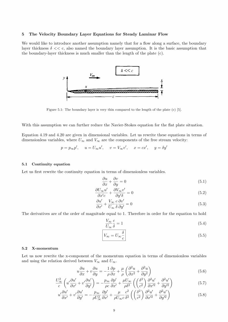
5 The Velocity Boundary Layer Equations for Steady Laminar Flow
We would like to introduce another assumption namely that for a flow along a surface, the boundarylayer thickness δ << c, also named the boundary layer assumption. It is the basic assumption thatthe boundary-layer thickness is much smaller than the length of the plate (c).
Figure 5.1: The boundary layer is very thin compared to the length of the plate (c) [5].
With this assumption we can further reduce the Navier-Stokes equation for the flat plate situation.
Equation 4.19 and 4.20 are given in dimensional variables. Let us rewrite these equations in terms ofdimensionless variables, where U∞ and V∞ are the components of the free stream velocity:
p = p∞p′, u = U∞u
′, v = V∞v′, x = cx′, y = δy′
5.1 Continuity equation
Let us first rewrite the continuity equation in terms of dimensionless variables.
∂u
∂x+∂v
∂y= 0 (5.1)
∂U∞u′
∂x′c+∂V∞v
′
∂y′δ= 0 (5.2)
∂u′
∂x′+V∞U∞
c
δ
∂v′
∂y′= 0 (5.3)
The derivatives are of the order of magnitude equal to 1. Therefore in order for the equation to hold
V∞U∞
c
δ= 1 (5.4)
V∞ = U∞δ
c(5.5)
5.2 X-momentum
Let us now rewrite the x-component of the momentum equation in terms of dimensionless variablesand using the relation derived between V∞ and U∞.
u∂u
∂x+ v
∂u
∂y= −1
ρ
∂p
∂x+µ
ρ
(∂2u
∂x2+∂2u
∂y2
)(5.6)
U2∞c
(u′∂u′
∂x′+ v′
∂u′
∂y′
)= −p∞
ρc
∂p′
∂x′+µU∞ρδ2
((δ2
c2
)∂2u′
∂x′2+∂2u′
∂y′2
)(5.7)
u′∂u′
∂x′+ v′
∂u′
∂y′= − p∞
ρU2∞
∂p′
∂x′+
µ
ρU∞c
c2
δ2
((δ2
c2
)∂2u′
∂x′2+∂2u′
∂y′2
)(5.8)
9
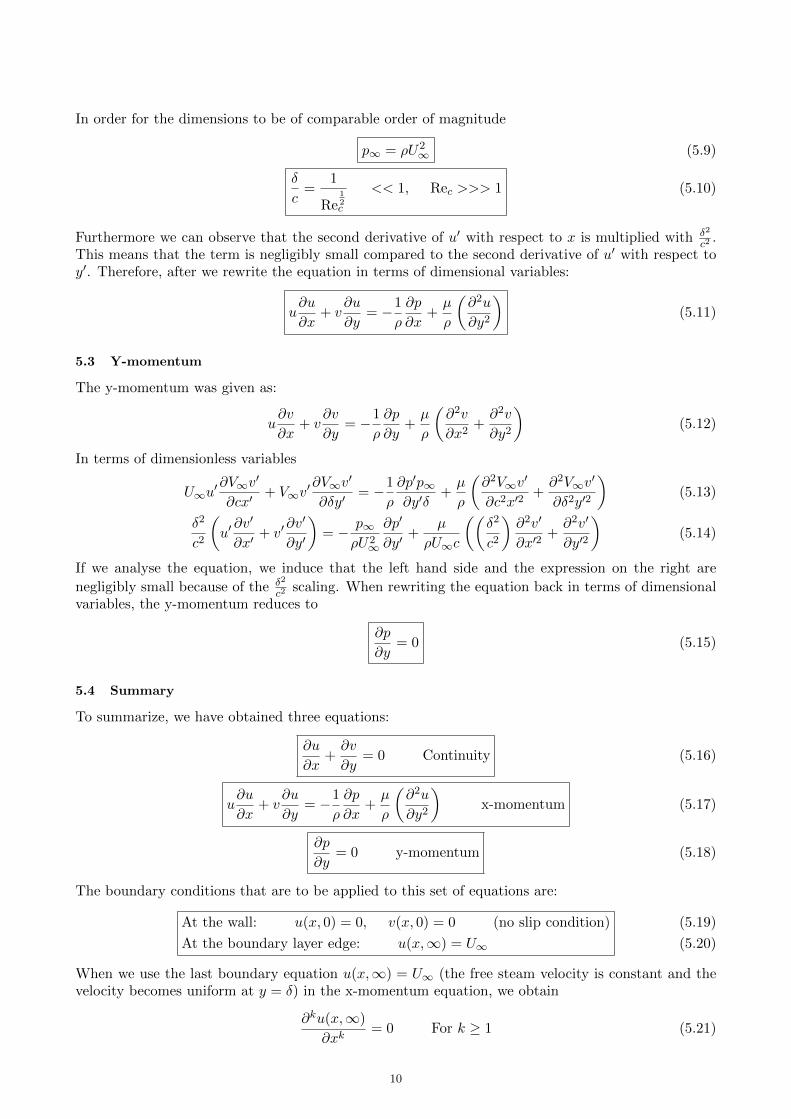
In order for the dimensions to be of comparable order of magnitude
p∞ = ρU2∞ (5.9)
δ
c=
1
Re12c
<< 1, Rec >>> 1 (5.10)
Furthermore we can observe that the second derivative of u′ with respect to x is multiplied with δ2
c2.
This means that the term is negligibly small compared to the second derivative of u′ with respect toy′. Therefore, after we rewrite the equation in terms of dimensional variables:
u∂u
∂x+ v
∂u
∂y= −1
ρ
∂p
∂x+µ
ρ
(∂2u
∂y2
)(5.11)
5.3 Y-momentum
The y-momentum was given as:
u∂v
∂x+ v
∂v
∂y= −1
ρ
∂p
∂y+µ
ρ
(∂2v
∂x2+∂2v
∂y2
)(5.12)
In terms of dimensionless variables
U∞u′∂V∞v
′
∂cx′+ V∞v
′∂V∞v′
∂δy′= −1
ρ
∂p′p∞∂y′δ
+µ
ρ
(∂2V∞v
′
∂c2x′2+∂2V∞v
′
∂δ2y′2
)(5.13)
δ2
c2
(u′∂v′
∂x′+ v′
∂v′
∂y′
)= − p∞
ρU2∞
∂p′
∂y′+
µ
ρU∞c
((δ2
c2
)∂2v′
∂x′2+∂2v′
∂y′2
)(5.14)
If we analyse the equation, we induce that the left hand side and the expression on the right are
negligibly small because of the δ2
c2scaling. When rewriting the equation back in terms of dimensional
variables, the y-momentum reduces to
∂p
∂y= 0 (5.15)
5.4 Summary
To summarize, we have obtained three equations:
∂u
∂x+∂v
∂y= 0 Continuity (5.16)
u∂u
∂x+ v
∂u
∂y= −1
ρ
∂p
∂x+µ
ρ
(∂2u
∂y2
)x-momentum (5.17)
∂p
∂y= 0 y-momentum (5.18)
The boundary conditions that are to be applied to this set of equations are:
At the wall: u(x, 0) = 0, v(x, 0) = 0 (no slip condition)
At the boundary layer edge: u(x,∞) = U∞
(5.19)
(5.20)
When we use the last boundary equation u(x,∞) = U∞ (the free steam velocity is constant and thevelocity becomes uniform at y = δ) in the x-momentum equation, we obtain
∂ku(x,∞)
∂xk= 0 For k ≥ 1 (5.21)
10
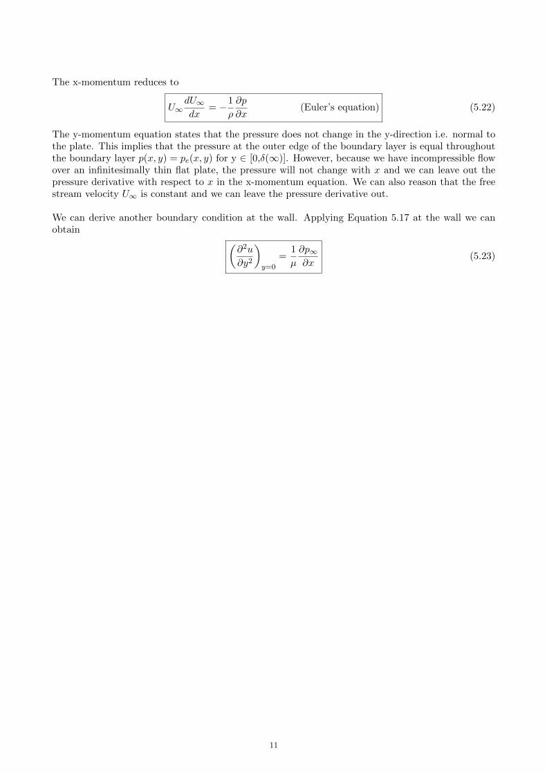
The x-momentum reduces to
U∞dU∞dx
= −1
ρ
∂p
∂x(Euler’s equation) (5.22)
The y-momentum equation states that the pressure does not change in the y-direction i.e. normal tothe plate. This implies that the pressure at the outer edge of the boundary layer is equal throughoutthe boundary layer p(x, y) = pe(x, y) for y ∈ [0,δ(∞)]. However, because we have incompressible flowover an infinitesimally thin flat plate, the pressure will not change with x and we can leave out thepressure derivative with respect to x in the x-momentum equation. We can also reason that the freestream velocity U∞ is constant and we can leave the pressure derivative out.
We can derive another boundary condition at the wall. Applying Equation 5.17 at the wall we canobtain (
∂2u
∂y2
)y=0
=1
µ
∂p∞∂x
(5.23)
11
12
6 The Solution of the Velocity Boundary Layer Equations for Steady, Laminar Flow
6.1 The Blasius equation
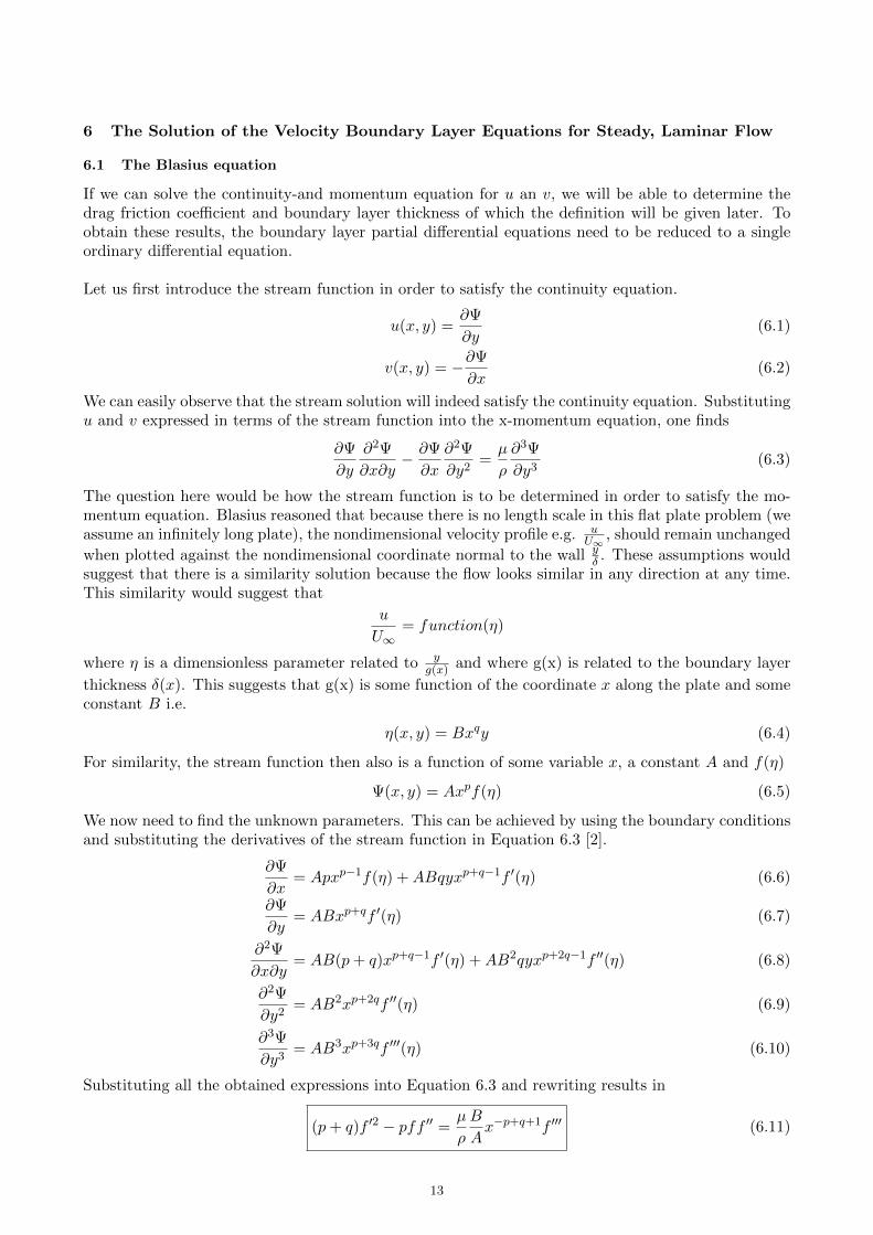
If we can solve the continuity-and momentum equation for u an v, we will be able to determine thedrag friction coefficient and boundary layer thickness of which the definition will be given later. Toobtain these results, the boundary layer partial differential equations need to be reduced to a singleordinary differential equation.
Let us first introduce the stream function in order to satisfy the continuity equation.
u(x, y) =∂Ψ
∂y(6.1)
v(x, y) = −∂Ψ
∂x(6.2)
We can easily observe that the stream solution will indeed satisfy the continuity equation. Substitutingu and v expressed in terms of the stream function into the x-momentum equation, one finds
∂Ψ
∂y
∂2Ψ
∂x∂y− ∂Ψ
∂x
∂2Ψ
∂y2=µ
ρ
∂3Ψ
∂y3(6.3)
The question here would be how the stream function is to be determined in order to satisfy the mo-mentum equation. Blasius reasoned that because there is no length scale in this flat plate problem (weassume an infinitely long plate), the nondimensional velocity profile e.g. u
U∞, should remain unchanged
when plotted against the nondimensional coordinate normal to the wall yδ . These assumptions would
suggest that there is a similarity solution because the flow looks similar in any direction at any time.This similarity would suggest that
u
U∞= function(η)
where η is a dimensionless parameter related to yg(x) and where g(x) is related to the boundary layer
thickness δ(x). This suggests that g(x) is some function of the coordinate x along the plate and someconstant B i.e.
η(x, y) = Bxqy (6.4)
For similarity, the stream function then also is a function of some variable x, a constant A and f(η)
Ψ(x, y) = Axpf(η) (6.5)
We now need to find the unknown parameters. This can be achieved by using the boundary conditionsand substituting the derivatives of the stream function in Equation 6.3 [2].
Substituting all the obtained expressions into Equation 6.3 and rewriting results in
(p+ q)f ′2 − pff ′′ = µ
ρ
B
Ax−p+q+1f ′′′ (6.11)
13
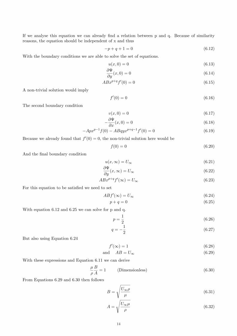
If we analyse this equation we can already find a relation between p and q. Because of similarityreasons, the equation should be independent of x and thus
−p+ q + 1 = 0 (6.12)
With the boundary conditions we are able to solve the set of equations.
u(x, 0) = 0 (6.13)
∂Ψ
∂y(x, 0) = 0 (6.14)
ABxp+qf ′(0) = 0 (6.15)
A non-trivial solution would imply
f ′(0) = 0 (6.16)
The second boundary condition
v(x, 0) = 0 (6.17)
−∂Ψ
∂x(x, 0) = 0 (6.18)
−Apxp−1f(0)−ABqyxp+q−1f ′(0) = 0 (6.19)
Because we already found that f ′(0) = 0, the non-trivial solution here would be
f(0) = 0 (6.20)
And the final boundary condition
u(x,∞) = U∞ (6.21)
∂Ψ
∂y(x,∞) = U∞ (6.22)
ABxp+qf ′(∞) = U∞ (6.23)
For this equation to be satisfied we need to set
ABf ′(∞) = U∞ (6.24)
p+ q = 0 (6.25)
With equation 6.12 and 6.25 we can solve for p and q.
p =1
2(6.26)
q = −1
2(6.27)
But also using Equation 6.24
f ′(∞) = 1 (6.28)
and AB = U∞ (6.29)
With these expressions and Equation 6.11 we can derive
µ
ρ
B
A= 1 (Dimensionless) (6.30)
From Equations 6.29 and 6.30 then follows
B =
√U∞ρ
µ(6.31)
A =
√U∞µ
ρ(6.32)
14
We gave now obtained all the unknown parameters and can substitute them in the momentum equationto obtain the third order ordinary differential equation (with its boundary conditions).
2f ′′′ + ff ′ = 0
f(0) = 0
f ′(0) = 0
f ′(∞) = 1
(6.33)
(6.34)
(6.35)
(6.36)
With the expressions for the stream function and η:
Ψ(x, y) = f(η)
√U∞
µ
ρx, η(x, y) = y
√U∞ρ
µx(6.37)
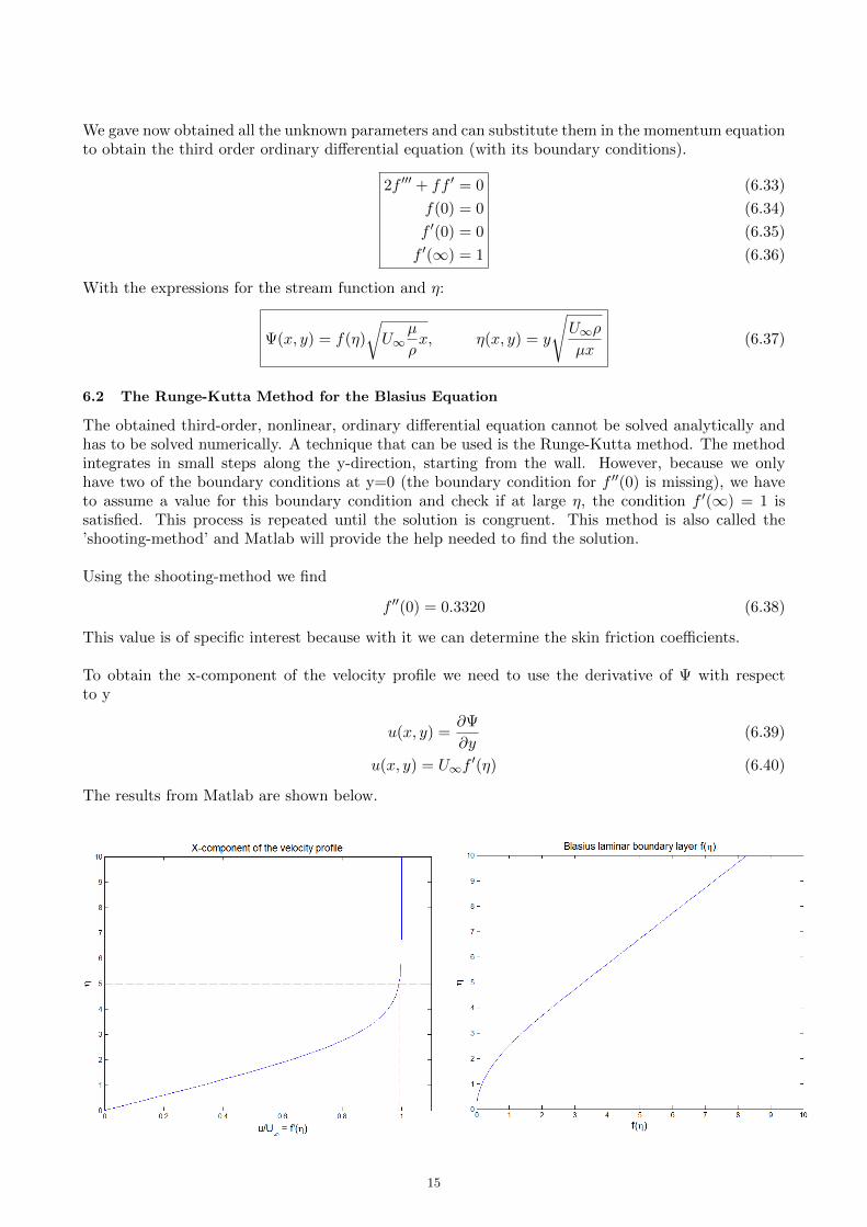
6.2 The Runge-Kutta Method for the Blasius Equation
The obtained third-order, nonlinear, ordinary differential equation cannot be solved analytically andhas to be solved numerically. A technique that can be used is the Runge-Kutta method. The methodintegrates in small steps along the y-direction, starting from the wall. However, because we onlyhave two of the boundary conditions at y=0 (the boundary condition for f ′′(0) is missing), we haveto assume a value for this boundary condition and check if at large η, the condition f ′(∞) = 1 issatisfied. This process is repeated until the solution is congruent. This method is also called the’shooting-method’ and Matlab will provide the help needed to find the solution.
Using the shooting-method we find
f ′′(0) = 0.3320 (6.38)
This value is of specific interest because with it we can determine the skin friction coefficients.
To obtain the x-component of the velocity profile we need to use the derivative of Ψ with respectto y
u(x, y) =∂Ψ
∂y(6.39)
u(x, y) = U∞f′(η) (6.40)
The results from Matlab are shown below.
15
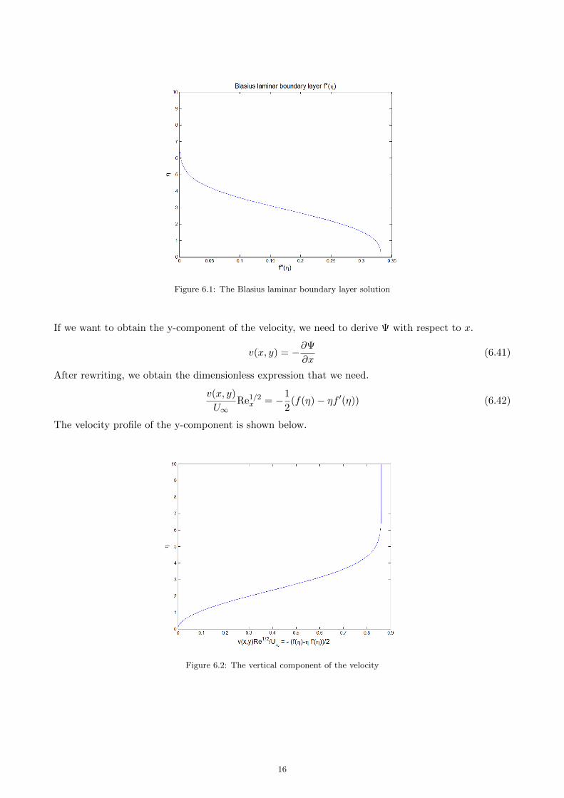
Figure 6.1: The Blasius laminar boundary layer solution
If we want to obtain the y-component of the velocity, we need to derive Ψ with respect to x.
v(x, y) = −∂Ψ
∂x(6.41)
After rewriting, we obtain the dimensionless expression that we need.
v(x, y)
U∞Re1/2x = −1
2(f(η)− ηf ′(η)) (6.42)
The velocity profile of the y-component is shown below.
Figure 6.2: The vertical component of the velocity
16
6.3 The Skin Friction Coefficient
With the results obtained by solving the Blasius equation we can now find further results such as theskin friction coefficients. The local skin friction coefficient is defined as
cf ≡τw
12ρU
2∞
(6.43)
And the wall shear stress τw is defined as
τw ≡ µ(∂u
∂y
)y=0
(6.44)
We can use Equation 6.40 to find
u(x, y) = U∞f′(η) (6.45)
∂u
∂y= U∞
df ′(η)
dy(6.46)
∂u
∂y= U∞
√U∞ρ
µxf ′′(η) (6.47)
So that
τw = U∞
√U∞ρµ
xf ′′(0) (6.48)
Substituting the obtained expression back into the local skin friction equation:
cf =
√U∞ρµx
12ρU
2∞f ′′(0) (6.49)
cf = 2
õ
U∞ρxf ′′(0) (6.50)
cf =2f ′′(0)
Re1/2x
(6.51)
Where Rex is the local Reynolds number. With the obtained approximation for f”(0) we find anexpression for the local skin friction coefficient.
cf (x) =0.664
Re1/2x
=0.664
Re1/2c
(xc
)−1/2(6.52)
The skin friction coefficient as function of the coordinate along the wall for a laminar air flow is plottedin Figure 6.3.
17
Figure 6.3: The local skin friction coefficient for laminar flow
From this expression we observe that the local skin friction coefficient is proportional to Re−1/2c and(
xc
)−1/2. The latter means that as the distance x increases from the leading edge, the local skin friction
coefficient decreases. We can now derive the total skin friction coefficient on the top of the flat plateby integrating the local skin friction coefficient from x=0 to x=c.
Cf =1
c
∫ c
0cfdx (6.53)
Cf =1.328
Re1/2c
(6.54)
Rec is the Reynolds number of the entire plate, meaning that the total skin friction coefficient decreasesas the Reynolds number increases.
6.4 The Boundary Layer Thickness
We are now able to derive the expression for the approximated boundary layer thickness using thedefinition of η.
η = y
√U∞ρ
µx(6.55)
Because the approximation is congruent, a point needs to be defined at which we choose that theboundary layer ends. We will define this as:
u/U∞ = 0.99 (6.56)
The calculation that was made with Matlab shows that η = 4.92 for u/U∞ = 0.99 (this can also beobserved in the first graph of Figure 6.1).
η = δ
√U∞ρ
µx= 4.92 (6.57)
δ(x) =4.92x
Re1/2x
(6.58)
δ
c=
4.92(xc
)1/2Re
1/2c
(6.59)
18
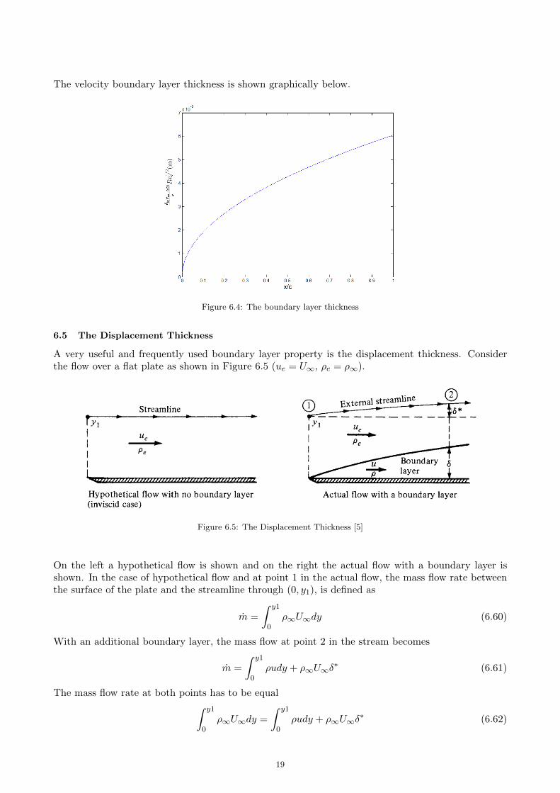
The velocity boundary layer thickness is shown graphically below.
Figure 6.4: The boundary layer thickness
6.5 The Displacement Thickness
A very useful and frequently used boundary layer property is the displacement thickness. Considerthe flow over a flat plate as shown in Figure 6.5 (ue = U∞, ρe = ρ∞).
Figure 6.5: The Displacement Thickness [5]
On the left a hypothetical flow is shown and on the right the actual flow with a boundary layer isshown. In the case of hypothetical flow and at point 1 in the actual flow, the mass flow rate betweenthe surface of the plate and the streamline through (0, y1), is defined as
m =
∫ y1
0ρ∞U∞dy (6.60)
With an additional boundary layer, the mass flow at point 2 in the stream becomes
m =
∫ y1
0ρudy + ρ∞U∞δ
∗ (6.61)
The mass flow rate at both points has to be equal∫ y1
0ρ∞U∞dy =
∫ y1
0ρudy + ρ∞U∞δ
∗ (6.62)
19
Rewriting yields
δ∗ =
∫ y1
0
(1− ρu
ρ∞U∞
)dy (6.63)
For incompressible flow, the equation becomes
δ∗ =
∫ y1
0
(1− u
U∞
)dy (6.64)
We also know that uU∞
= f ′(η) and then
δ∗ =
õx
ρU∞
∫ η1
0
(1− f ′(η)
)dη (6.65)
δ∗ =
õx
ρU∞[η1 − f(η1)] (6.66)
If we then consider points of η1 anywhere above the boundary-layer we observe with Matlab thatη1 − f(η1) is constant at a value of approximately 1.72. Therefore the approximated value of thedisplacement thickness can be expressed as
δ∗(x) =1.72x
Re1/2x
(6.67)
δ∗
c=
1.72(xc
)1/2Re
1/2c
(6.68)
Equation 6.68 indicates that the displacement thickness is proportional to the square root of x. More-over, when we compare this result with the result in Equation 6.59 we find that for the flat-plateboundary layer δ∗ = 0.35δ.
6.6 The Momentum Thickness
Another useful boundary-layer property is the momentum thickness. Figure 6.6 will help to understandthis concept.
Figure 6.6: The Momentum Thickness [5]
Let us consider a mass flow through a segment dy which is given as
dm = ρudy (6.69)
The momentum flow through this segment is then
dy = dm u = ρu2dy (6.70)
20
In a segment in the free stream, the momentum flow is
dy = dm U∞ = ρU∞udy (6.71)
And the decrement of momentum flow can be defined as
ρu(U∞ − u)dy (6.72)
The integral from the wall to the streamline passing through (0,y1) will then give the total decrement.∫ y1
0ρu(U∞ − u)dy (6.73)
Let us now assume that the missing momentum flow in the free stream is ρ∞U2∞θ. Then again,
according to momentum conservation we can state
ρ∞U2∞θ =
∫ y1
0ρu(U∞ − u)dy (6.74)
θ =
∫ y1
0
ρu
ρ∞U∞
(1− u
U∞
)dy (6.75)
We can again use the relation uU∞
= f ′(η).
θ =
õx
U∞
∫ η1
0f ′(η)(1− f ′(η))dη (6.76)
Equation 6.76 can only be evaluated numerically and results in
θ(x) =0.664x
Re1/2x
(6.77)
θ
c=
0.664(xc
)1/2Re
1/2c
(6.78)
We find that the momentum thickness is proportional to the square root of x. We can also find, usingpreviously obtained relations that for the flat-plate boundary layer θ = 0.13δ and θ = 0.39δ∗.
21
22
7 The von Karman and Pohlhausen Approximate Solution
Apart from the Blasius solution of the boundary-layer equation, it is also possible to use the vonKarman (and Pohlhausen) solution to determine the properties of the boundary layer from someapproximated velocity profile of the flow above an infinitesimally thin flat plate. Let us return to theboundary-layer equations in Section 5.4.
∂u
∂x+∂v
∂y= 0 Continuity (7.1)
u∂u
∂x+ v
∂u
∂y= −1
ρ
dp∞dx
+µ
ρ
(∂2u
∂y2
)x-momentum (7.2)
At the wall: u(x, 0) = 0, v(x, 0) = 0 (no slip condition)
At the boundary layer edge: u(x,∞) = U∞
And∂ku
∂yk(x,∞) = 0
(7.3)
(7.4)
(7.5)
Furthermore at the boundary layer edge:
U∞dU∞dx
= −1
ρ
dp∞dx
(Euler’s equation) (7.6)
Using Equation 7.2 and 7.6, the x-momentum becomes
u∂u
∂x+ v
∂u
∂y= U∞
dU∞dx
+ ν
(∂2u
∂y2
) (µ
ρ= ν
)(7.7)
u∂u
∂x+ v
∂u
∂y− U∞
dU∞dx− ν
(∂2u
∂y2
)= 0 (7.8)
We can rewrite the left hand side using some mathematical manipulation.
(u− U∞)
(∂u
∂x+∂v
∂y
)= 0 (Continuity equation) (7.9)
u∂u
∂x+ u
∂v
∂y− U∞
∂u
∂x− U∞
∂v
∂y= 0 (7.10)
We can use this to rewrite expression 7.8.
u∂u
∂x+ v
∂u
∂y− U∞
dU∞dx− ν
(∂2u
∂y2
)+
(u∂u
∂x+ u
∂v
∂y− U∞
∂u
∂x− U∞
∂v
∂y= 0
)= 0 (7.11)
Rewriting Equation 7.11 will eventually lead to
ν∂2u
∂y2= (U∞ − u)
dU∞dx
+ u∂(U∞ − u)
∂x+ (U∞ − u)
∂u
∂x(7.12)
ν∂2u
∂y2= (U∞ − u)
dU∞dx
+∂
∂x(u(U∞ − u)) (7.13)
Now integrate with respect to y and using the relation that(∂u∂y
)y=0
= τwµ :
ν∂u
∂y y=0
=
∫ y1
0
{(U∞ − u)
dU∞dx
+∂
∂x(u(U∞ − u))
}dy (7.14)
ν∂u
∂y y=0
= ντ
µ=τ
ρ(7.15)
τ
ρ=dU∞dx
∫ y1
0(U∞ − u)dy +
d
dx
∫ y1
0u(U∞ − u)dy (7.16)
τ
ρ=dU∞dx
U∞
∫ y1
0(1− u
U∞)dy +
d
dxU2∞
∫ y1
0
u
U∞(1− u
U∞)dy (7.17)
23
Let us now recall the equations for the displacement thickness and momentum integral for incom-pressible flow, Equation 6.75 and 6.63. We can substitute Equation 6.75 and 6.63 to obtain the vonKarman momentum integral for incompressible flow
τ
ρ=dU∞dx
U∞δ∗ +
d
dxU2∞θ (7.18)
In order to obtain an equation for the boundary-layer thickness δ(x)we need to assume a velocity pro-file. A second, third and (Pohlhausen’s) fourth-order polynomial function will be used to approximatethe velocity profile.
7.1 Second Order Velocity Profile
A second-order, quadratic function is of the form
u(x, y) = a+ by + cy2 (7.19)
Three boundary conditions are needed to determine the coefficients.
At the wall : u(0) = 0
At the boundary layer edge : u(δ) = U∞ and∂u(δ)
∂y= 0
Applying the boundary conditions we find the unknown parameters
a = 0 b =2U∞δ(x)
c = − U∞δ(x)
(7.20)
so thatu(x, y)
U∞= 2
y
δ
(1− 1
2
y
δ
)(7.21)
We have obtained a result similar to the Blasius equation except that here η = yδ(x) .
u(η)
U∞= 2η − η2 for η ∈ [0, 1] and (7.22)
u(η)
U∞= 1 for η ≥ 1. (7.23)
Subsequently, we want to derive an expression for the boundary-layer thickness. Let us return toEquation 7.18.
τ
ρ=dU∞dx
U∞δ∗ +
d
dxU2∞θ (7.24)
Analysing the equation, we observe that the free stream velocity U∞ is constant (i.e. for the Blasiussolution) and the equation reduces to
τwρ
=d
dxU2∞θ (7.25)
If we derive the expressions for τw and θ (which has the boundary layer thickness included), we obtainan expression for the boundary-layer thickness δ(x).
θ =
∫ y1
0
u
U∞
(1− u
U∞
)dy (7.26)
θ
δ=
∫ y,1δ
0
u
U∞
(1− u
U∞
)dη (7.27)
Substituting Equation 7.22 in Equation 7.27 we obtain
θ
δ=
2
15(7.28)
24
The wall shear stress is defined as
τw = µ
(∂u
∂y
)y=0
(7.29)
For this quadratic function τw becomes
τw =2µU∞δ(x)
(7.30)
Combining Equation 7.30 and 7.28 in Equation 7.25
2µU∞δ(x)
= ρU2∞dδ
dx
2
15(7.31)
We can now rearrange and integrate to derive the boundary layer thickness.∫ δ
0δ′(x)δdx =
∫ x
0
15µ
ρU∞dx (7.32)
δ(x) =
√30x
Re1/2x
(7.33)
δ(x) =5.48x
Re1/2x
(7.34)
δ
c=
5.48(xc
)1/2Re
1/2c
(7.35)
Another parameter we want to derive is the local skin friction coefficient cf (x) which is defined as
cf =τ
12ρU
2∞
(7.36)
And the total skin friction coefficients
Cf =1
c
∫ c
0cfdx (7.37)
Substituting the obtained expressions of the boundary-layer thickness δ in the stress tensor τ andsubsequently in the local skin friction coefficient we derive the expressions for the local and total skinfriction coefficients.
cf (x) =0.73
Re1/2x
=0.73
Re1/2c
(xc
)−1/2(7.38)
Cf =1.46
Re1/2c
(7.39)
25
7.2 Third Order Velocity Profile
Let us now consider a third-order, cubic function
u(x, y) = a+ by + cy2 + dy3 (7.40)
The function can also be written in terms of η
u(x, y)
U∞= a+ bη + cη2 + dη3 η =
y
δ(7.41)
To determine the coefficients, we will need an additional boundary condition. Let us examine thex-momentum. On the wall (y=0), we previously derived
−1
ρ
∂p
∂x+ ν
∂2u
∂y2 y=0
= 0 (7.42)
Substituting Equation 7.6 in 7.42 we obtain the additional boundary condition(∂2u
∂y2
)y=0
= −U∞ν
dU∞dx
(7.43)
Let us define
−U∞ν
dU∞dx
= −Λ (7.44)
The boundary conditions are
f(0) = 0 f(1) = 1 f ′(1) = 0 f ′′(0) = −Λ (7.45)
Solving the set of equations, we obtain
a = 0 b =3
2+
1
4Λ c = −1
2Λ d = −1
2+
1
4Λ (7.46)
so thatu(x, y)
U∞=
3
2η − 1
2η3 + Λ
1
4η(η − 1)2 for η ∈ [0, 1] and (7.47)
u(η)
U∞= 1 for η ≥ 1. (7.48)
Using the same steps as for the second-order velocity profile, we obtain the expressions for the mo-mentum integral, wall shear stress and boundary layer thickness. We again use the assumption thatthe free stream velocity is constant i.e. the Blasius solution (Λ = 0).
θ
δ=
234
1680(7.49)
τw =3µU∞2δ(x)
(7.50)
δ(x) =4.64x
Re1/2x
(7.51)
δ
c=
4.64(xc
)1/2Re
1/2c
(7.52)
With the derived expressions of the boundary-layer thickness and wall shear stress, we can derive theskin friction coefficients
cf (x) =0.647
Re1/2x
=0.647
Re1/2c
(xc
)−1/2(7.53)
Cf =1.29
Re1/2c
(7.54)
26
7.3 Pohlhausen’s Fourth Order Velocity Profile
We will finally consider a fourth-order, quartic velocity profile which was used by Pohlhausen.
u(x, y)
U∞= a+ bη + cη2 + dη3 + eη4 (7.55)
The additional boundary condition comes from the boundary condition at the edge of the boundary
layer where all the derivatives (∂ku∂yk
=0 for k≥1) because the velocity becomes uniform. Therefore, all
the boundary conditions are:
f(0) = 0 f(1) = 1 f ′(1) = 0 f ′′(1) = 0 f ′′(0) = Λ (7.56)
Solving the set of equations gives us the coefficients
a = 0 b =1
6Λ + 2 c = −1
2Λ d =
1
2Λ− 2 e = −1
6Λ + 1 (7.57)
u(x, y)
U∞= 2η − 2η3 + η4 + Λ
1
6η(η − 1)3 for η ∈ [0, 1] and (7.58)
u(η)
U∞= 1 for η ≥ 1. (7.59)
The equations for the momentum integral, wall shear stress and boundary-layer thickness (whileassuming a constant free stream velocity, Λ = 0) then become
θ
δ=
37
315(7.60)
τs =2µU∞δ(x)
(7.61)
δ(x) =5.84x
Re1/2x
(7.62)
δ
c=
5.84(xc
)1/2Re
1/2c
(7.63)
With the derived expressions of the boundary layer thickness and stress tensor we can derive the skinfriction coefficients
cf (x) =0.685
Re1/2x
=0.685
Re1/2c
(xc
)−1/2(7.64)
Cf =1.37
Re1/2c
(7.65)
27
28
8 Comparison of the Blasius and von Karman Approximations
The boundary-layer thickness and velocity profiles are compared below.
Blasius : δ(x) =4.92x
Re1/2x
u(x, y) = U∞f′(η)
Second-Order : δ(x) =5.48x
Re1/2x
u(x, y)
U∞= 2η − η2
Third-Order : δ(x) =4.64x
Re1/2x
u(x, y)
U∞=
3
2η − 1
2η3 + Λ
1
4η(η − 1)2
Fourth-Order : δ(x) =5.84x
Re1/2x
u(x, y)
U∞= 2η − 2η3 + η4 + Λ
1
6η(η − 1)3
In order to compare the Blasius solution to the von Karman solutions we first need to find a relationbetween the two.
Blasius : η = y
√U∞ρ
µx=y
xRe1/2x (8.1)
von Karman : η =y
δ(x)(8.2)
When we substitute the boundary layer thickness, obtained from the Blasius solution, into Equation8.2, we obtain the relation
ηBlasius = 4.92η (8.3)
In Figure 8.1, η is plotted against uU∞
and the four velocity profiles are compared.
Figure 8.1: Comparison of the velocity profiles
The second-order velocity profile appears to be closest to the Blasius solution. The third and fourth-order models deviate substantially from the Blasius equation.
29
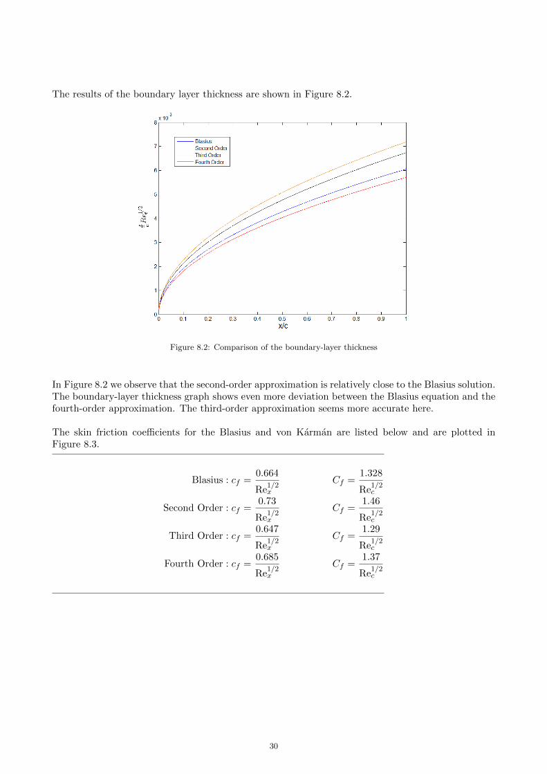
The results of the boundary layer thickness are shown in Figure 8.2.
Figure 8.2: Comparison of the boundary-layer thickness
In Figure 8.2 we observe that the second-order approximation is relatively close to the Blasius solution.The boundary-layer thickness graph shows even more deviation between the Blasius equation and thefourth-order approximation. The third-order approximation seems more accurate here.
The skin friction coefficients for the Blasius and von Karman are listed below and are plotted inFigure 8.3.
Blasius : cf =0.664
Re1/2x
Cf =1.328
Re1/2c
Second Order : cf =0.73
Re1/2x
Cf =1.46
Re1/2c
Third Order : cf =0.647
Re1/2x
Cf =1.29
Re1/2c
Fourth Order : cf =0.685
Re1/2x
Cf =1.37
Re1/2c
30
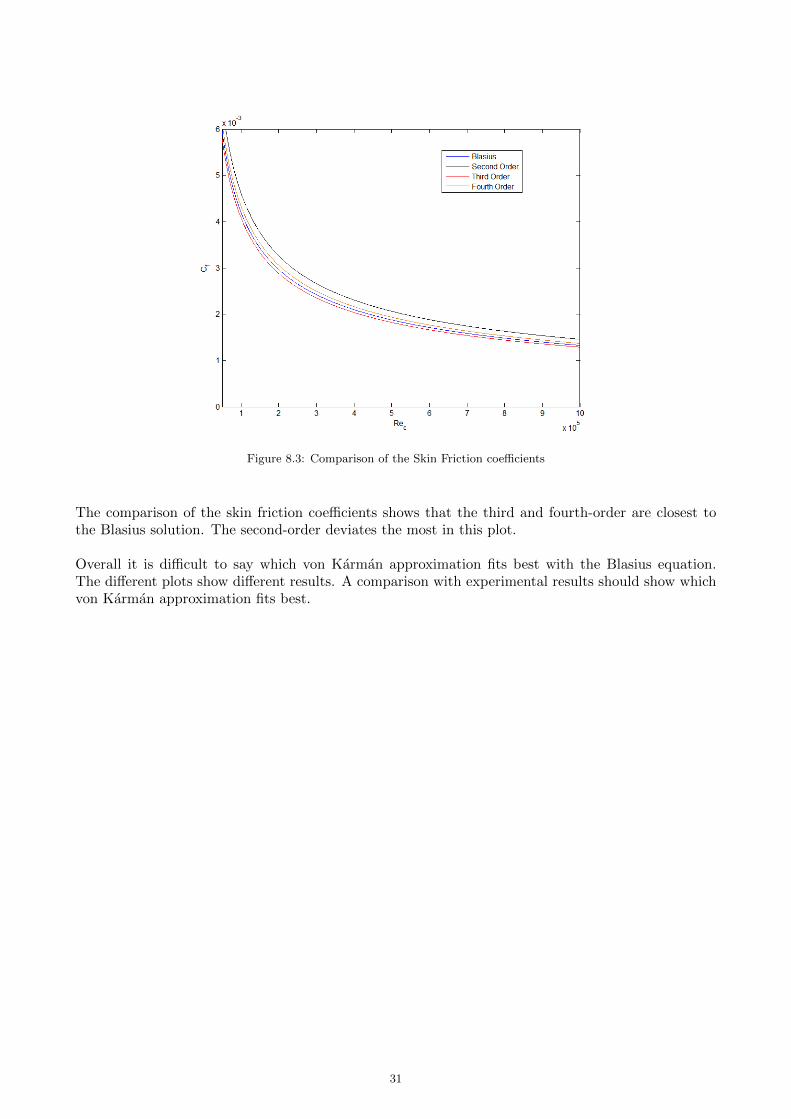
Figure 8.3: Comparison of the Skin Friction coefficients
The comparison of the skin friction coefficients shows that the third and fourth-order are closest tothe Blasius solution. The second-order deviates the most in this plot.
Overall it is difficult to say which von Karman approximation fits best with the Blasius equation.The different plots show different results. A comparison with experimental results should show whichvon Karman approximation fits best.
31
32
9 The Velocity Boundary Layer for Turbulent Flow
Turbulence is still an unsolved problem in fluid dynamics. The formulas used to describe turbulencehere are therefore based on data from experiments combined with theory.
9.1 The Boundary Layer Thickness
The velocity boundary layer thickness for incompressible turbulent flow over a flat plate is given as
δ(x) ∼=0.37x
Re1/5x
(9.1)
δ
c∼=
0.37
Re1/5c
(xc
)4/5(9.2)
Instead of the velocity boundary layer thickness to be proportional to x−1/2 for laminar flow, itis proportional to x−4/5 for turbulent flow. Figure 9.1 shows the difference between laminar andturbulent flow for an air flow of 15m/s i.e. Rec=1 · 106.
Figure 9.1: The comparison of the velocity boundary-layers for laminar and turbulent flow Rec=1 · 106
9.2 The Skin Friction Coefficients
The local and total skin friction drag coefficient for incompressible turbulent flow over an infinitesimallyflat plate are given as
cf (x) ∼=0.0592
Re1/5c
(xc
)−1/5(9.3)
Cf ∼=0.074
Re1/5c
(9.4)
Note that for the laminar flow the skin friction coefficient was proportional to Re−1/2c and for turbulent
flow it is proportional to Re−1/5c .
33
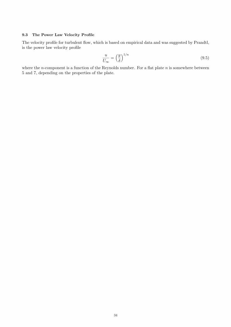
9.3 The Power Law Velocity Profile
The velocity profile for turbulent flow, which is based on empirical data and was suggested by Prandtl,is the power law velocity profile
u
U∞=(yδ
)1/n(9.5)
where the n-component is a function of the Reynolds number. For a flat plate n is somewhere between5 and 7, depending on the properties of the plate.
34
10 Transitional Flow
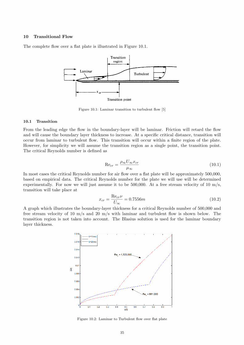
The complete flow over a flat plate is illustrated in Figure 10.1.
Figure 10.1: Laminar transition to turbulent flow [5]
10.1 Transition
From the leading edge the flow in the boundary-layer will be laminar. Friction will retard the flowand will cause the boundary layer thickness to increase. At a specific critical distance, transition willoccur from laminar to turbulent flow. This transition will occur within a finite region of the plate.However, for simplicity we will assume the transition region as a single point, the transition point.The critical Reynolds number is defined as
Recr =ρ∞U∞xcr
µ∞(10.1)
In most cases the critical Reynolds number for air flow over a flat plate will be approximately 500,000,based on empirical data. The critical Reynolds number for the plate we will use will be determinedexperimentally. For now we will just assume it to be 500,000. At a free stream velocity of 10 m/s,transition will take place at
xcr =Recrν
U∞= 0.7556m (10.2)
A graph which illustrates the boundary-layer thickness for a critical Reynolds number of 500,000 andfree stream velocity of 10 m/s and 20 m/s with laminar and turbulent flow is shown below. Thetransition region is not taken into account. The Blasius solution is used for the laminar boundarylayer thickness.
Figure 10.2: Laminar to Turbulent flow over flat plate
35
There are a number of factors that can have an influence on the boundary layer transition [3]:
1. The Streamwise Pressure Gradient
2. The Surface Roughness
3. The Turbulence Level in the Wind Tunnel
4. The Wall Temperature
5. Suction
6. Vibrations of the plate itself
7. Acoustic Disturbances
In current understandings, transition to turbulence is caused by the development of unstable Tollmien-Schlichting waves. Initially, disturbances in the boundary-layer will develop into unstable modes whichwill grow downstream inside the boundary layer. When these modes reach a certain amplification, theflow becomes turbulent. This amplification factor is used in the modelling of the flow over the plate inXFOIL and is further discussed in section 11.4. However, detailed theory on the Tollmien-Schlichtingwill not be further addressed in this report.
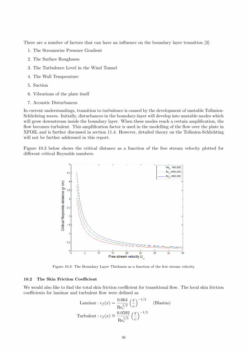
Figure 10.3 below shows the critical distance as a function of the free stream velocity plotted fordifferent critical Reynolds numbers.
Figure 10.3: The Boundary Layer Thickness as a function of the free stream velocity
10.2 The Skin Friction Coefficient
We would also like to find the total skin friction coefficient for transitional flow. The local skin frictioncoefficients for laminar and turbulent flow were defined as
Laminar : cf (x) =0.664
Re1/2c
(xc
)−1/2(Blasius)
Turbulent : cf (x) ∼=0.0592
Re1/5c
(xc
)−1/5
36
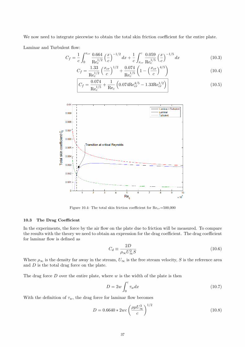
We now need to integrate piecewise to obtain the total skin friction coefficient for the entire plate.
Laminar and Turbulent flow:
Cf =1
c
∫ xcr
0
0.664
Re1/2c
(xc
)−1/2dx+
1
c
∫ c
xcr
0.059
Re1/5c
(xc
)−1/5dx (10.3)
Cf =1.33
Re1/2c
(xcrc
)1/2+
0.074
Re1/5c
(1−
(xcrc
)4/5)(10.4)
Cf =0.074
Re1/5c
+1
Rec
(0.074Re4/5cr − 1.33Re1/2cr
)(10.5)
Figure 10.4: The total skin friction coefficient for Recr=500,000
10.3 The Drag Coefficient
In the experiments, the force by the air flow on the plate due to friction will be measured. To comparethe results with the theory we need to obtain an expression for the drag coefficient. The drag coefficientfor laminar flow is defined as
Cd ≡2D
ρ∞U2∞S
(10.6)
Where ρ∞ is the density far away in the stream, U∞ is the free stream velocity, S is the reference areaand D is the total drag force on the plate.
The drag force D over the entire plate, where w is the width of the plate is then
D = 2w
∫ c
0τwdx (10.7)
With the definition of τw, the drag force for laminar flow becomes
D = 0.6640 ∗ 2wc
(ρµU3
∞c
)1/2
(10.8)
37
Substituting the obtained expression for D into the equation for the drag coefficient and rewriting willresult in the total drag force coefficient of both sides of the plate
Cd =2.656
Re1/2c
(10.9)
For Turbulent flow, the drag coefficient is given as
Cd =0.148
Re1/5c
(10.10)
38
11 Flow over a Flat Plate Predicted by XFOIL
The plate that is used in the experiments is modelled using XFOIL (Version 6.99). Appendix A showsthe dimensions of the plate. The leading edge is defined by a Hermite polynomial shape (set up byH.W.M. Hoeijmakers) in combination with a square root function and has a length of 5% of the entireplate. The trailing edge has a very sharp and fragile profile, defined by the last 70% of a NACA4-series with a length of 20% of the plate. The plate has a thickness of 10mm, width of 890mm andlength of 1000mm. The Matlab code which is used to generate the coordinates for XFOIL is shownin Appendix B.
The critical amplification factor in XFOIL is set to 5, which is most suitable for the silent WindTunnel of the UT as will be described in section 11.4.
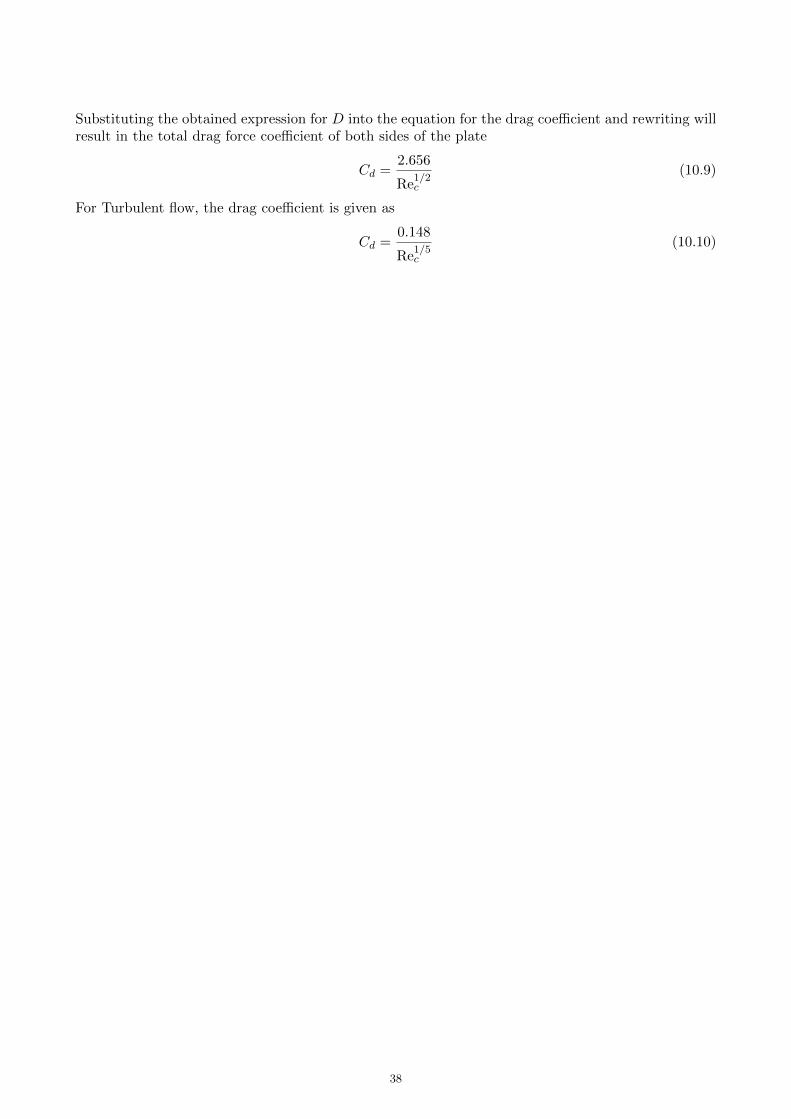
11.1 The Leading Edge
The shape of the leading edge is described by a Hermite polynomial in combination with a squareroot function. The Hermite polynomial function is continuous in function value, slope, curvature andcurvature derivative. The root function completes the nose and connects it with the middle section ofthe plate. The function of the plate in an (x,y) coordinate system is defined as
y(ξ) =t
2
[b1ξ
1/2 + b2ξ3/2 + f(0)P1(ξ) + f ′(0)Q1(ξ) + f(1)P2(ξ) + f ′(1)Q2(ξ)
](11.1)
With
ξ =x− xnose
xplate − xnose b1 =
√8
∆x
t
(−R(0))
tb2 = −16 + 5b1
P1(ξ) = (1− ξ)2(1 + 2ξ)
P2(ξ) = 1− P1(ξ)
Q1(ξ) = (1− ξ)2ξQ2(ξ) = −ξ2(1− ξ)
f(0) = 0
f(1) = 1− b1 − b2
f ′(0) = 3− 15
8b1 −
3
8b2
f ′(1) = −1
2b1 −
3
2b2
Figure 11.1: The Leading Edge
There are two free parameters, the length of the nose (∆x) and the radius of the leading edge (R(0)).These values are made dimensionless with the thickness t of the plate. The choice made for the presentplate is
∆x
t= 5
R(0)
t= 0.2
The resulting shape of the leading edge is shown in Appendix A.
39
11.2 The Trailing Edge
The shape of the trailing edge is determined by the last 70% of a NACA 4-series and is 20% of theplate length. The NACA 4-series has a constant value and slope, but not a constant curvature. Thefunction describing the coordinates is defined as:
y
c= ± t
2
[0.2969
√x
c− 0.1260
(xc
)− 0.3516
(xc
)2+ 0.2843
(xc
)3− 0.01015
(xc
)4](11.2)
With x = 0 the location of the leading edge of the airfoil and x = c its trailing edge. The resultingshape is shown in Appendix A.
40
11.3 Point Distribution
It was chosen to use a non-uniform point distribution, where the leading edge and trailing edge haveabout 4.5 times more points than the middle section. The maximum number of points you can useis 1000 (XFOIL does not allow more). The Matlab code in Appendix B shows how many points (i.e.panels) were eventually used for each section.
11.4 Turbulence Level of the Silent Wind Tunnel
It is given that the turbulence level (i.e. the environmental disturbance) of the Silent Wind Tunnel isdetermined as approximately 0.25% [9]. However, XFOIL uses the semi-empirical en method (based onlinear stability theory) and it works with the amplification factor N (based on the Tollmien-Schlichtinginstability). The relation between the N-factor and turbulence level is [4]
NT = −8.34− 2.4 ln(Tu) (11.3)
The relation is graphically shown in Figure 11.2 and only holds for Tu>0.1%. It is based on Mack’srelationship who proposed to (empirically) relate the N factor to the turbulence level.
Figure 11.2: The en method related to the turbulence level according to Mack’s relationship [6]
Using Equation 11.3 we find that for a turbulence level of 0.25%, the N factor is 5.02.
11.5 The Pressure Coefficient
First, we are interested in the dimensionless pressure coefficient [5] because it will give insight inthe pressure gradient of the plate. The pressure gradient will indicate if the plate behaves as ainfinitesimally flat plate. For a perfect flat plat Cp = 0 all along the surface of the plate. The pressurecoefficient is defined as
Cp ≡p− p∞12ρ∞U
2∞
(11.4)
and it describes the dimensionless pressure throughout the flow. Where p is the static pressure at thepoint of interest, p∞ is the free stream static pressure and ρ∞ is the free stream density. The pressurecoefficient describes the relative pressure throughout the flow. When the pressure coefficient is zero,the pressure is the same as in the free stream velocity. For Rec = 5 · 105 the pressure coefficient alongthe plate is shown in Figure 11.3.
41
Figure 11.3: The pressure coefficient along the plate for a flow of Rec = 5 · 105
The graph shows us that the pressure coefficient along the plate is very close to zero which confirmsthat we can assume that the pressure along the plate is close to the free stream pressure and thevelocity outside the boundary layer is close to the free stream velocity. The stagnation point (whereCp=1) can also be observed. Moreover, at the leading edge we observe that the pressure coefficientbecomes negative indicating that the pressure becomes lower than the free stream pressure and thevelocity exceeds the free stream value ( U
U∞≈ 1.2). The results for a Reynolds number of 1 · 106 and
2 · 106 are shown in Figure 11.4 and 11.5 respectively
Figure 11.4: The pressure coefficient along the plate for a flow of Rec = 1 · 106
42
Figure 11.5: The pressure coefficient along the plate for a flow of Rec = 1.5 · 106
The figures indicate that for higher Reynolds numbers, the flow can still be considered to be verysimilar to the flow along a flat plate of infinitesimally thickness placed flush in a uniform free stream.Therefore the Blasius solution should (with some accuracy) describe the flow over this plate.
43
11.6 The Skin Friction Coefficient
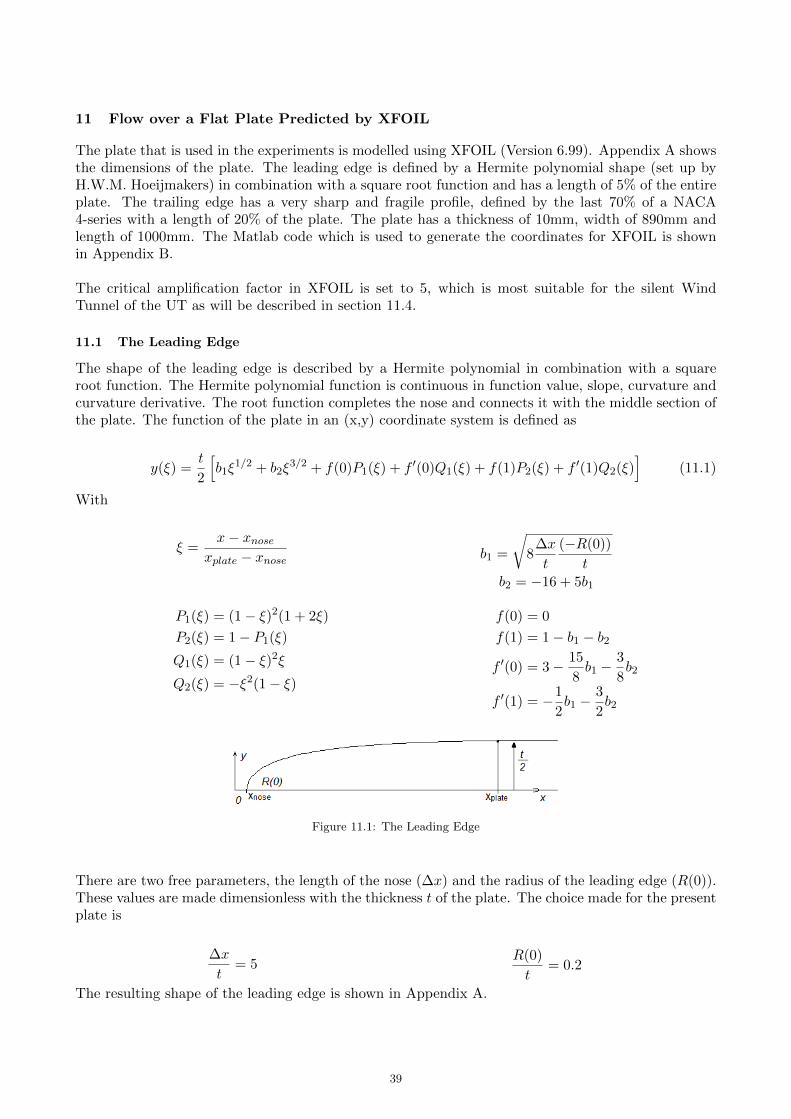
Figure 11.6: The local skin friction coefficient for various Reynolds numbers
The local skin friction coefficient is plotted in Figure 11.6 for various Reynolds numbers. The Reynoldsnumber of Rec = 5 · 105 shows the skin friction coefficient with full laminar flow. Higher Reynoldsnumbers show a transition from laminar to turbulent flow. The distance of the transition point fromthe leading edge decreases for increasing Reynolds numbers; Rec=1e6, Rec=1.5e6 and Rec=2e6 resultin xtr/c = 0.49, 0.24 and 0.15 respectively.
11.6.1 XFOIL compared to the (Blasius) Theory
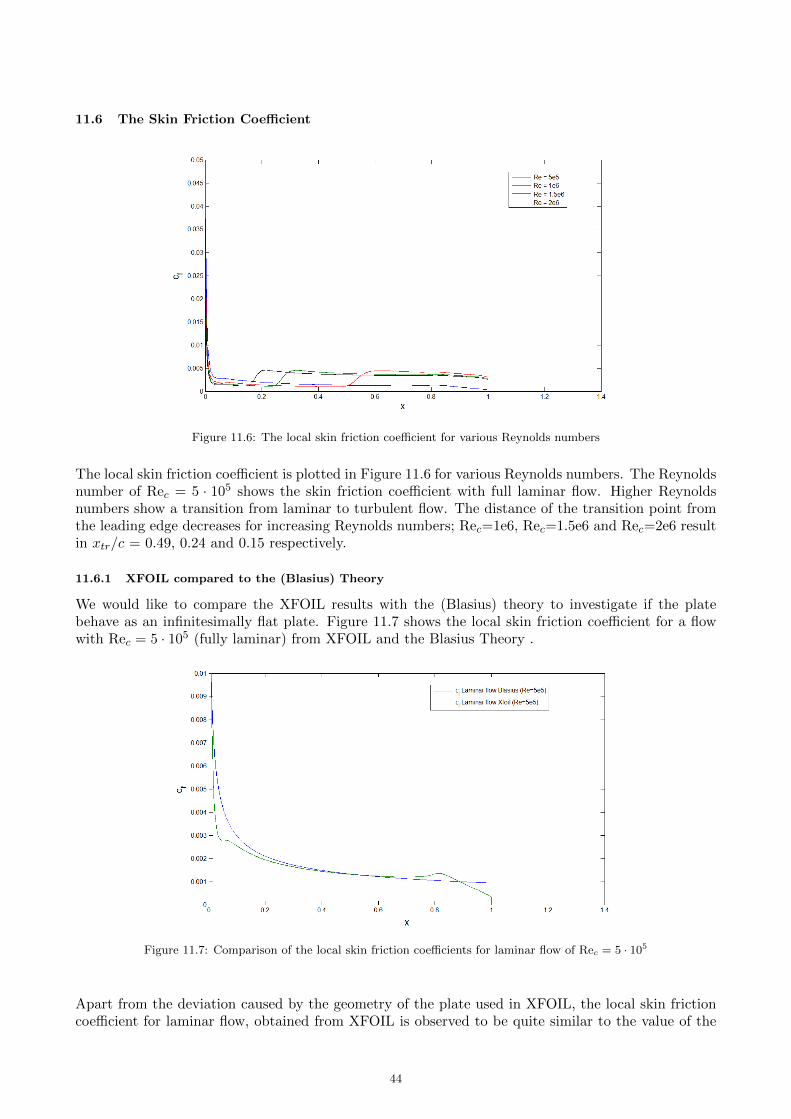
We would like to compare the XFOIL results with the (Blasius) theory to investigate if the platebehave as an infinitesimally flat plate. Figure 11.7 shows the local skin friction coefficient for a flowwith Rec = 5 · 105 (fully laminar) from XFOIL and the Blasius Theory .
Figure 11.7: Comparison of the local skin friction coefficients for laminar flow of Rec = 5 · 105
Apart from the deviation caused by the geometry of the plate used in XFOIL, the local skin frictioncoefficient for laminar flow, obtained from XFOIL is observed to be quite similar to the value of the
44
skin friction coefficient according to Blasius’ solution. The result for a (predominantly) turbulent flowwith Rec = 2 · 106 is shown in Figure 11.8.
Figure 11.8: Comparison of the local skin friction coefficients for turbulent flow of Rec = 2 · 106
Again, we observe great similarity between the local skin friction coefficient obtained from the (Blasius)theory and that predicted by XFOIL. This indicates that the designed plate should aerodynamicallybehave as an infinitesimally flat plate and the derived theory should describe the flow over the plate.
11.7 Boundary Layer Properties
The boundary layer properties are considered next, i.e. the boundary layer thickness, the displacementthickness and momentum thickness obtained from XFOIL. The results are shown below. The dashedline indicates the boundary-layer thickness δ/c.
Figure 11.9: The displacement thickness, boundary layer thickness and momentum thickness for a flow with Rec = 5 ·105.
45
Figure 11.10: The displacement thickness, boundary-layer thickness and momentum thickness for a flow with Rec = 1·106.
Figure 11.10 and 11.9 clearly show the relations between the boundary layer thickness, displacementthickness and momentum thickness as described in section 6.5 and 6.6. The properties for a flowwith Rec = 5 · 105 are mostly governed by laminar flow except for the forced transition caused bythe change of geometry. It is hard to quantitatively compare these XFOIL results with the obtainedtheory (about the boundary-layer thickness etc.), but they seem quite similar.
Figure 11.11: The displacement thickness, boundary-layer thickness and momentum thickness for a flow with Rec =1.5 · 106.
A final result is obtained for a flow with Rec = 1.5 ·106. We observe that the difference between θ andδ∗ becomes smaller in a turbulent flow. This can also be observed if we were to plot the kinematicshape factor Hk which gives the relation between θ and δ∗. However, because we are also able toobserve this in these plots and the kinematic shape factor is not of interest in this research. Therefore,the kinematic shape factor graph is not shown.
46
12 Experimental Details
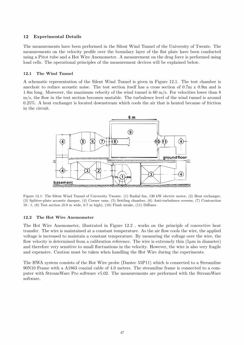
The measurements have been performed in the Silent Wind Tunnel of the University of Twente. Themeasurements on the velocity profile over the boundary layer of the flat plate have been conductedusing a Pitot tube and a Hot Wire Anemometer. A measurement on the drag force is performed usingload cells. The operational principles of the measurement devices will be explained below.
12.1 The Wind Tunnel
A schematic representation of the Silent Wind Tunnel is given in Figure 12.1. The test chamber isanechoic to reduce acoustic noise. The test section itself has a cross section of 0.7m x 0.9m and is1.8m long. Moreover, the maximum velocity of the wind tunnel is 60 m/s. For velocities lower than 8m/s, the flow in the test section becomes unstable. The turbulence level of the wind tunnel is around0.25%. A heat exchanger is located downstream which cools the air that is heated because of frictionin the circuit.
Figure 12.1: The Silent Wind Tunnel of University Twente. (1) Radial fan, 130 kW electric motor, (2) Heat exchanger,(3) Splitter-plate acoustic damper, (4) Corner vane, (5) Settling chamber, (6) Anti-turbulence screens, (7) Contraction10 : 1, (8) Test section (0.9 m wide, 0.7 m high), (10) Flush intake, (11) Diffuser.
12.2 The Hot Wire Anemometer
The Hot Wire Anemometer, illustrated in Figure 12.2 , works on the principle of convective heattransfer. The wire is maintained at a constant temperature. As the air flow cools the wire, the appliedvoltage is increased to maintain a constant temperature. By measuring the voltage over the wire, theflow velocity is determined from a calibration reference. The wire is extremely thin (5µm in diameter)and therefore very sensitive to small fluctuations in the velocity. However, the wire is also very fragileand expensive. Caution must be taken when handling the Hot Wire during the experiments.
The HWA system consists of the Hot Wire probe (Dantec 55P11) which is connected to a Streamline90N10 Frame with a A1863 coaxial cable of 4.0 meters. The streamline frame is connected to a com-puter with StreamWare Pro software v5.02. The measurements are performed with the StreamWaresoftware.
47
Figure 12.2: Hot Wire Anemometer [6]
12.3 Hot Wire Anemometer Calibration
Before every measurement, the HWA has to be calibrated. During the calibration, the Hot Wire isplaced in an uniform flow with known velocity. The flow is generated by blowing through a nozzle witha pressure supply (see Appendix C2). The pressure in the nozzle is measured with a Betz manometer.With Bernoulli’s equation the velocity is then determined. With the StreamWare software, the HWAis then calibrated. It is important that the calibration is performed in the wind tunnel in order forthe results to be consistent. Moreover, the probe has to be in the same position (i.e. facing the flowin the same attitude) as it will be in the measurements.
12.4 The Pitot Tube
A Pitot tube is also used to measure the flow velocity. By measuring the static and stagnation pressureof the flow, the flow velocity can be obtained.
Bernoulli’s equation for an incompressible flowstates that along a streamline
p1 +1
2ρU2
1 = p2 +1
2ρU2
2
where point 1 is the stagnation point, point 2 anarbitrary static point and U the flow velocity. Be-cause the velocity in the stagnation point is zero,the equation becomes
p1 = p2 +1
2ρU2
2
The flow velocity at point 2 can then be determineby measuring the pressure difference and using thedensity of the flow:
U2 =
√2(p1 − p2)
ρFigure 12.3: Pitot Tube Principle [7]
48
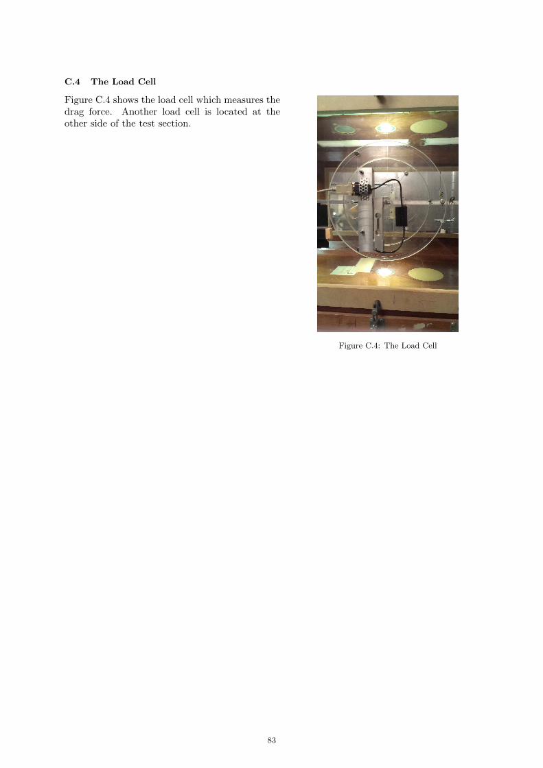
12.5 The Load Cell
The experimental set-up is shown in Figure 12.4. The plate is suspended by 4 rods in total. A rodthrough the middle of the plate pushes against both load cells. The second load cell is located onthe other side of the test section. A load cell works on the principle of a strain gauge which underdeformation will have a different electrical resistance. The load cell is calibrated by suspending aweight with known load to the plate through a pulley. Before the measurement, the voltage offset iszeroed. The measured voltage can then be used to calculate the exerted force.
Figure 12.4: The set-up of the plate in the Wind Tunnel
49
50
13 Experimental Results
13.1 The Velocity Boundary-Layer Measurement with the Pitot tube
Initial measurements on the velocity profile have been performed with a Pitot tube which was custommade. The Pitot tube has a diameter of 3mm. Consequently, the velocity profile could not be mea-sured closer than about 1.6mm from the surface of the plate.
The velocity in the wind tunnel is measured with a fixed Pitot tube in the wind tunnel which mea-sures both static and stagnation pressure to determine the velocity in the wind tunnel. However, thePitot tube which is used to determine the stagnation pressure in the boundary layer over the flatplat cannot measure the static pressure. Therefore, we will have a different offset in the measurementwith respect to the velocity determination with the Pitot tube in the wind tunnel. This is the resultof the different offset on each individual port of the measurement apparatus. However, because theresults are made nondimensional, the pressure measured with Pitot 2 in the free stream, compared tothe boundary-layer measurement should give valid results without an offset error. This is because wedivide the free stream velocity with the boundary layer velocity, effectively dividing out the offset.
Moreover, it is important to note that the results have been corrected due to a different static pressureof the flow below the plate. It was measured that there is a streamwise pressure gradient below theplate. Therefore, the static pressure of the Pitot tube in the wind tunnel, used to determine the flowvelocity, could not be used. The static pressure of the closest pressure orifice (orifice 3) in the windtunnel was therefore used to determine the dynamic pressure and consequently the velocity profiles.The results of the streamwise distribution of the pressure in the test section of the wind tunnel canbe found in section 13.4
The results of the Pitot tube measurements are shown in Figure 13.1-13.6 below. The velocity profileis measured in steps of 0.1mm and at a distance of x=0.62m from the leading edge. A comparisonis made with the Blasius solution and Pohlhausen’s 4th order approximation. Pohlhausen’s 4th or-der approximation is plotted because the velocity profile tends to show the 4th order behaviour athigher velocities (i.e. higher Reynolds numbers). Because the boundary layer is thinner at higherReynolds numbers, the region in the boundary layer in which measurements with the Pitot tubecan be performed decreases with increasing velocity. Moreover, the boundary layer thickness from themeasurements is determined with Matlab, using the criterion in Equation 6.56. To indicate a standarderror (of 0.1 mm) in the determination, the red lines are plotted.
51
Figure 13.1: The velocity profile as measured with the Pitot tube with Rex = 3.26 · 105 (U=8m/s).
Figure 13.1 also shows the instability of the Silent Wind Tunnel at low velocities.
Figure 13.2: The velocity profile as measured with the Pitot tube with Rex = 4.07 · 105 (U=10m/s).
52
Figure 13.3: The velocity profile as measured with the Pitot tube with Rex = 4.88 · 105 (U=12m/s).
Figure 13.4: The velocity profile as measured with the Pitot tube with Rex = 6.11 · 105 (U=15m/s).
53
Figure 13.5: The velocity profile as measured with the Pitot tube with Rex = 1.02 · 106 (U=25m/s).
We observe an unpredicted trend in the velocity profile. The shape of the velocity profile appears tocurve with increasing Reynolds number. The deviation can be caused by a combination of an errorin the boundary-layer thickness determination and some error in the determination of the free streamvelocity. A slight variation of 0.1m/s in the measured free stream velocity will result in a less curvedvelocity profile. It could also be caused by disturbances in the flow. Therefore the measurement witha free stream velocity of 25 m/s (Rex = 1.02 · 106) was repeated (at a different span of the plate) toverify the results. The resulting velocity profile of this second measurement in shown below.
54
Figure 13.6: The second measurement on the velocity profile as measured with the Pitot tube with Rex = 1.02 · 106
(U=25m/s).
The second velocity profile measurement seems much more in accordance with the Blasius Theory.However the difference between both measurements is striking. We found an indication that thevelocity measured with the Pitot tube varies in the span of the plate which could have caused theseresults. Therefore the pressure along the span of the plate was measured to verify the assumption.
55
13.1.1 The Stagnation Pressure along the Span of the Plate
The Pitot tube was placed along the span of the plate to measure the stagnation pressure. For everymeasurement point, the distance between the plate and Pitot tube was set identical. The measurementstarts at 5 cm from the center of the plate and ends at 15cm from the center of the plate. The pressurewas measured at 2.0 mm and 2.5 mm from the surface of the plate. The result of the measurement isshown in Figure 13.7.
Figure 13.7: The stagnation pressure along the span of the plate
The pressure measurement shows that the velocity is not constant along the span of the plate at themeasured velocity for 25 m/s (Rex = 1.02 · 106) and therefore the flow is not uniform in this direction.These changes are presumably due to anomalies of the surface of the plate, possibly also indicatingthe development of so-called turbulent wedges. The difference between the stagnation pressures is alsoplotted. The difference shows that when one would determine the velocity profiles at the measurementpoints, the resulting velocity profiles are not equal as Figure 13.5 and 13.6 already showed.
13.1.2 The Boundary-Layer Thickness
The boundary-layer thicknesses that are determined from the Pitot measurements are shown below.
Rexδx
Re1/2x (Blasius=4.92)
3.26 ·105 5.01
4.07 ·105 4.56
4.88 ·105 4.77
6.11 ·105 4.45
1.02 ·106 4.76 & 5.25
Table 1: The measured boundary layer thickness
56
13.1.3 Turbulent Flow Measurement
The velocity profile in a turbulent boundary layer has also been measured. The result is shown inFigure 13.8. Turbulence was induced with a turbulator strip placed just downstream of the leadingedge. With a very sensitive microphone it has been determined that there was indeed turbulent flow.However, the flow over the plate was not fully turbulent. A small area downstream of the leading edgestill showed laminar flow behaviour. The result of the turbulent flow measurement is compared withthe power law velocity profile. The 1/5th power law appears to fit the measurement results best.
Figure 13.8: The velocity profile as measured with the Pitot in a tripped boundary layer with Rex = 6.11·105 (U=15m/s).The boundary layer thickness is 9.3 mm.
57
13.2 The Velocity Boundary-Layer Measurement with the Hot Wire Anemometer
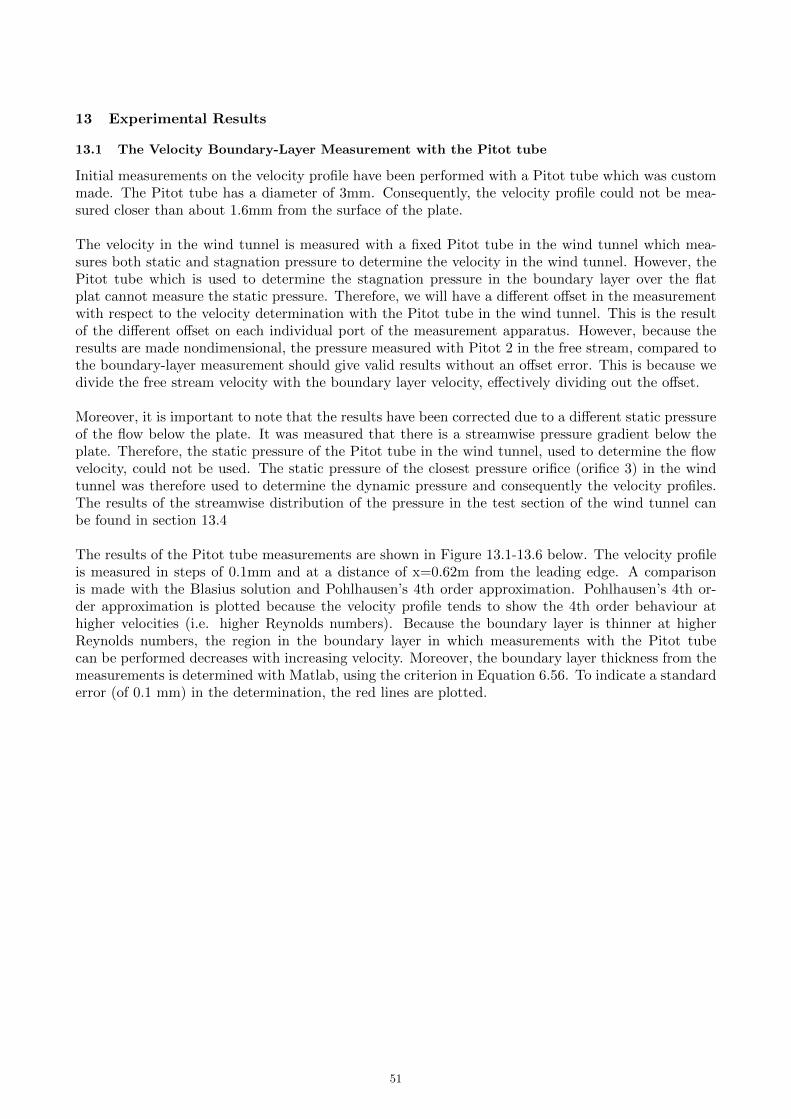
Figures 13.9 - 13.13 show the velocity profiles which have been measured with the HWA. The positionof the HWA relative to the leading edge is the same as the position of the Pitot tube, a distance ofx=0.62m from the leading edge. With the HWA it was very difficult to determine the distance fromthe plate since the HWA should not touch the plate. Therefore the HWA was placed increasinglycloser to the plate until the measured voltage increased again, indicating that the wire was losing heatto the plate. From this starting position, the velocity was determined in steps of 0.1mm. Becauseof the difficulty in measuring the exact distance, the results have been fitted to the velocity profileaccording to Blasius. This does not change the shape of the graph but only shifts it in the y-direction.
The measurements at U=8m/s and U=10m/s are plotted starting at a distance of 0.1mm from theplate. The measurements at U=12m/s, U=15m/s and U=25m/s are plotted starting at a distance of0.2mm from the plate. The measurements for U=12m/s and U=15m/s do not show the behaviourclose to the plate and thus the starting distance was set at a longer distance from the plate.
Figure 13.9: The velocity profile as measured with the Hot Wire with Rex = 3.26 · 105 (U=8m/s).
Figure 13.9 shows great similarity with the Blasius solution. The first few measurement points showthe effects of heat transfer to the plate which can also be observed in the U=10m/s and U=25m/smeasurement.
58
Figure 13.10: The velocity profile as measured with the Hot Wire with Rex = 4.07 · 105 (U=10m/s).
Figure 13.11: The velocity profile as measured with the Hot Wire with Rex = 4.88 · 105 (U=12m/s).
59
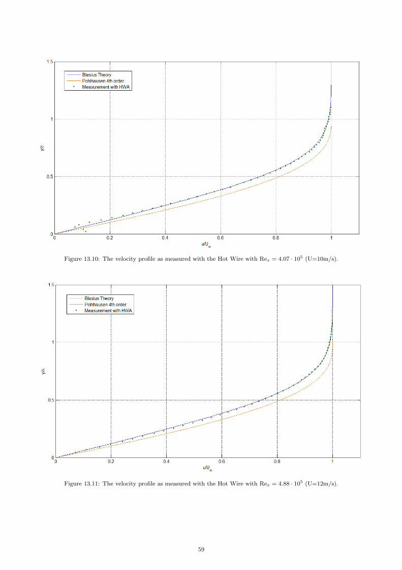
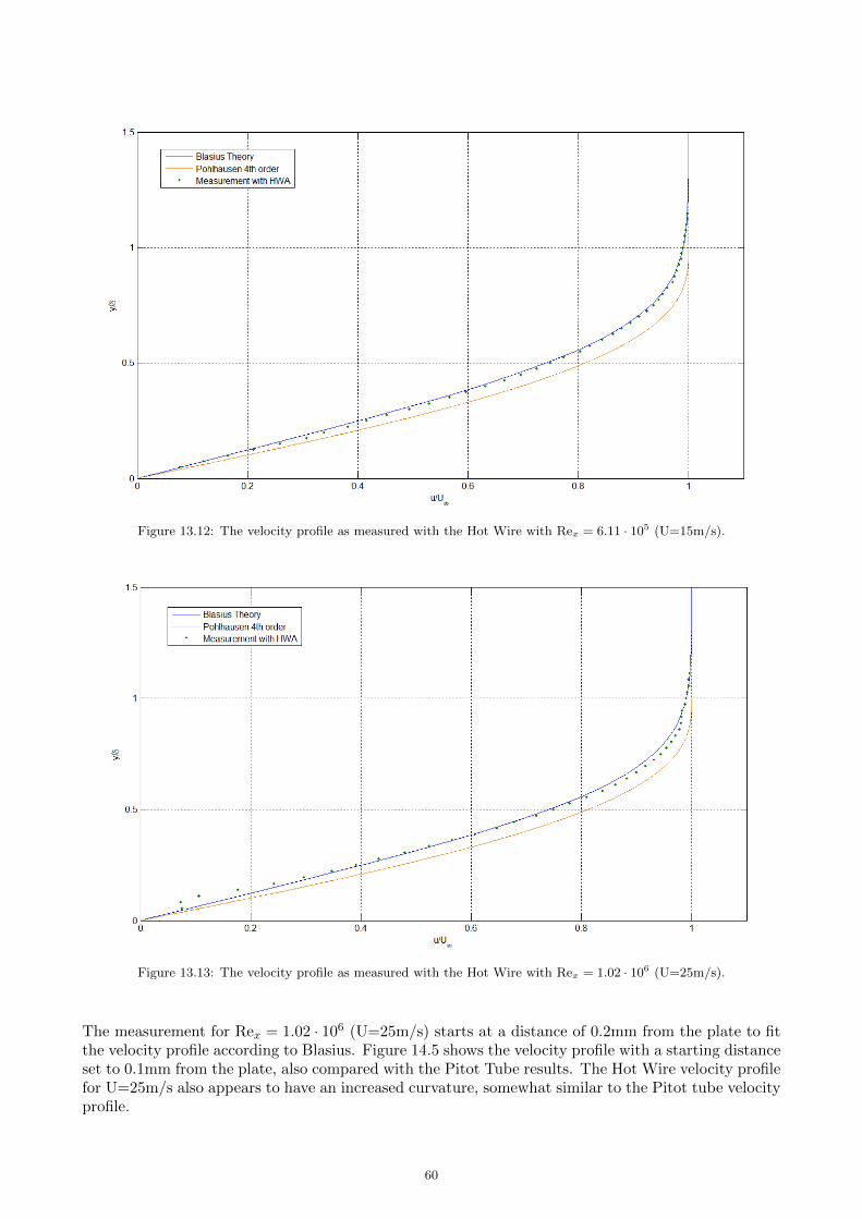
Figure 13.12: The velocity profile as measured with the Hot Wire with Rex = 6.11 · 105 (U=15m/s).
Figure 13.13: The velocity profile as measured with the Hot Wire with Rex = 1.02 · 106 (U=25m/s).
The measurement for Rex = 1.02 · 106 (U=25m/s) starts at a distance of 0.2mm from the plate to fitthe velocity profile according to Blasius. Figure 14.5 shows the velocity profile with a starting distanceset to 0.1mm from the plate, also compared with the Pitot Tube results. The Hot Wire velocity profilefor U=25m/s also appears to have an increased curvature, somewhat similar to the Pitot tube velocityprofile.
60
13.2.1 The Boundary Layer Thickness
The determined boundary layer thicknesses from the Hot Wire measurement are shown in the tablebelow. In general, the Hot Wire measurements are closer to the Blasius Theory than the Pitot tubemeasurements.
Rexδx
Re1/2x , Pitot δ
xRe
1/2x , Hot Wire
3.26 ·105 5.01 4.92
4.07 ·105 4.56 5.08
4.88 ·105 4.77 4.89
6.11 ·105 4.45 5.08
1.02 ·106 4.76 & 5.25 5.9
Table 2: The measured boundary layer thickness from both measurements (Blasius Theory = 4.92)
13.3 The Drag Force
The results of the drag force measurements are shown below. Information about the load cell, whichwas used to determine the drag force, can be found in Appendix C.4. The results show transitionat a quite high Reynolds number, which is not as expected. According to the theory and XFOILsimulations, the critical Reynolds number at which transition should occur is at approximately 500,000whereas in the present experiment transition occurs at a Reynolds number of about 3,000,0000. Apossible cause is the streamwise pressure gradient for which the results are represented in section 13.4.The measured drag coefficient for laminar flow is observed to be slightly higher than the value fromtheory, which is most likely caused by the interaction of the side walls of the wind tunnel with theboundary layer on the plate.
Figure 13.14: The drag coefficient measured using the load cells
Figure 13.14 shows two sets of measurements. One set in the lower Reynolds number range and a sec-ond set in the higher Reynolds number range, in which transition occurred. From these measurementswe conclude that the load cell is not very sensitive in the lower Reynolds number range, where it givesa lower output voltage. It was also observed that the load cell is very sensitive to small variations in
61
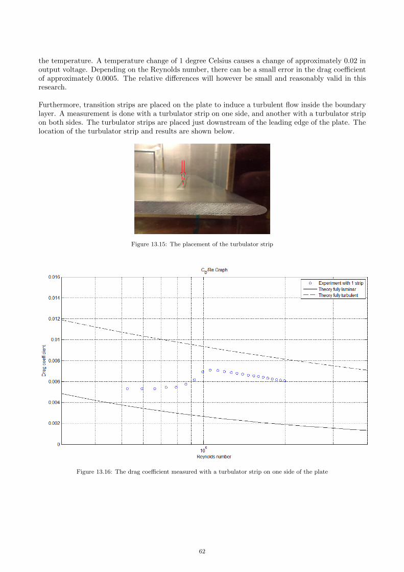
the temperature. A temperature change of 1 degree Celsius causes a change of approximately 0.02 inoutput voltage. Depending on the Reynolds number, there can be a small error in the drag coefficientof approximately 0.0005. The relative differences will however be small and reasonably valid in thisresearch.
Furthermore, transition strips are placed on the plate to induce a turbulent flow inside the boundarylayer. A measurement is done with a turbulator strip on one side, and another with a turbulator stripon both sides. The turbulator strips are placed just downstream of the leading edge of the plate. Thelocation of the turbulator strip and results are shown below.
Figure 13.15: The placement of the turbulator strip
Figure 13.16: The drag coefficient measured with a turbulator strip on one side of the plate
62
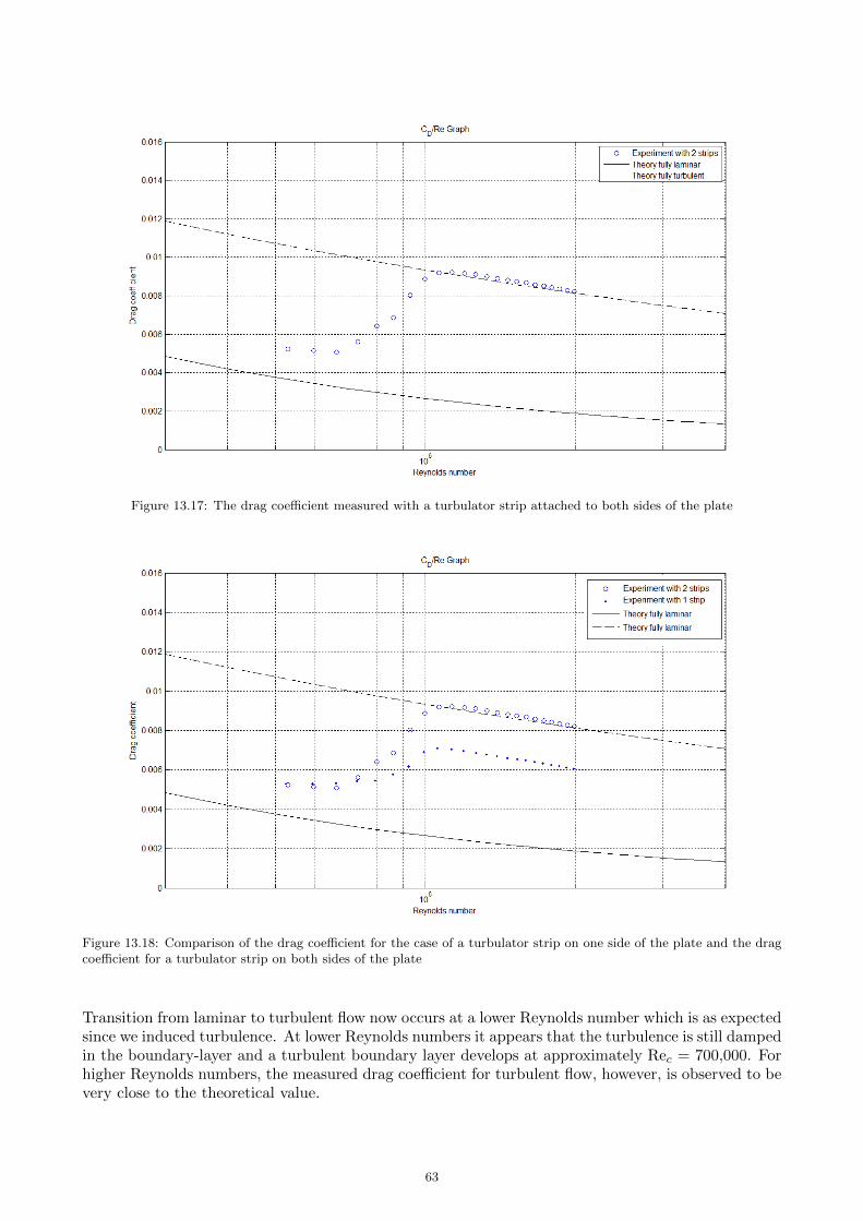
Figure 13.17: The drag coefficient measured with a turbulator strip attached to both sides of the plate
Figure 13.18: Comparison of the drag coefficient for the case of a turbulator strip on one side of the plate and the dragcoefficient for a turbulator strip on both sides of the plate
Transition from laminar to turbulent flow now occurs at a lower Reynolds number which is as expectedsince we induced turbulence. At lower Reynolds numbers it appears that the turbulence is still dampedin the boundary-layer and a turbulent boundary layer develops at approximately Rec = 700,000. Forhigher Reynolds numbers, the measured drag coefficient for turbulent flow, however, is observed to bevery close to the theoretical value.
63
13.4 The Streamwise Pressure Gradient in the Silent Wind Tunnel
The results of the drag force measurements gave rise to a number of possibilities that could havecaused the delayed transition. The most likely reasons are the turbulence level of the wind tunnel,acoustic disturbances or a change in streamwise pressure gradient. There has already been extensiveresearch in the turbulence level of the wind tunnel from which was concluded that the turbulence levelis around 0.25% [9]. In order for the turbulence level to have an influence on the delay of transition,the turbulence level would have to be very low (0.03%), which is highly unlikely. Because measuringacoustic disturbances was not possible, the possibility of a favourable streamwise pressure gradientwas investigated. Initially, numerical simulations were performed with XFOIL in order to investigatethe effects of a favourable pressure gradient.
13.4.1 XFOIL Simulations
To simulate a favourable pressure gradient in XFOIL, the plate was placed at a small positive angle ofattack. Figure 13.19 and 13.20 show an angle of attack of 0.5◦ and 1.0◦, respectively, which result ina small favourable pressure gradient along the lower surface of the plate. Table 3 shows the transitionpoint for various angles of attack.
Figure 13.19: The pressure coefficient obtained from XFOIL for the plate at an angle of attack of 0.50◦
64
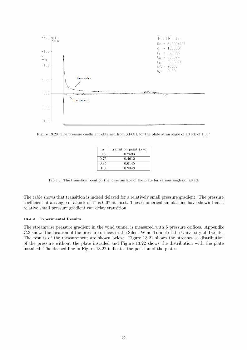
Figure 13.20: The pressure coefficient obtained from XFOIL for the plate at an angle of attack of 1.00◦
α transition point (x/c)
0.5 0.2593
0.75 0.4612
0.85 0.6145
1.0 0.9348
Table 3: The transition point on the lower surface of the plate for various angles of attack
The table shows that transition is indeed delayed for a relatively small pressure gradient. The pressurecoefficient at an angle of attack of 1◦ is 0.07 at most. These numerical simulations have shown that arelative small pressure gradient can delay transition.
13.4.2 Experimental Results
The streamwise pressure gradient in the wind tunnel is measured with 5 pressure orifices. AppendixC.3 shows the location of the pressure orifices in the Silent Wind Tunnel of the University of Twente.The results of the measurement are shown below. Figure 13.21 shows the streamwise distributionof the pressure without the plate installed and Figure 13.22 shows the distribution with the plateinstalled. The dashed line in Figure 13.22 indicates the position of the plate.
65
Figure 13.21: The streamwise distribution of the pressure in the Silent Wind Tunnel without the plate installed
Figure 13.22: The streamwise distribution of the pressure in the Silent Wind Tunnel with the plate installed
The measurement shows that the test section of the Silent Wind Tunnel has a pressure gradient whichis enhanced when the plate is installed. It is therefore possible that the pressure gradient is responsiblefor the delayed transition. Follow-up research should further investigate the effects of the streamwisepressure gradient on transition.
66
14 Comparison
In this chapter the velocity profiles obtained with the Pitot Tube and Hot Wire are compared. Theresults are compared for each free stream velocity. Figure 14.6 also shows the comparison of all theHot Wire measurements and Figure 14.7 shows the comparison of all the Pitot tube measurements.
Figure 14.1: Comparison of the results of the HWA, Pitot and Blasius velocity profiles for Rex = 3.26 · 105 (U=8m/s)
Figure 14.2: Comparison of the results of the HWA, Pitot and Blasius velocity profiles for Rex = 4.07 · 105 (U=10m/s)
67
Figure 14.3: Comparison of the results of the HWA, Pitot and Blasius velocity profiles for Rex = 4.88 · 105 (U=12m/s)
Figure 14.4: Comparison of the results of the HWA, Pitot and Blasius velocity profiles for Rex = 6.11 · 105 (U=15m/s)
68
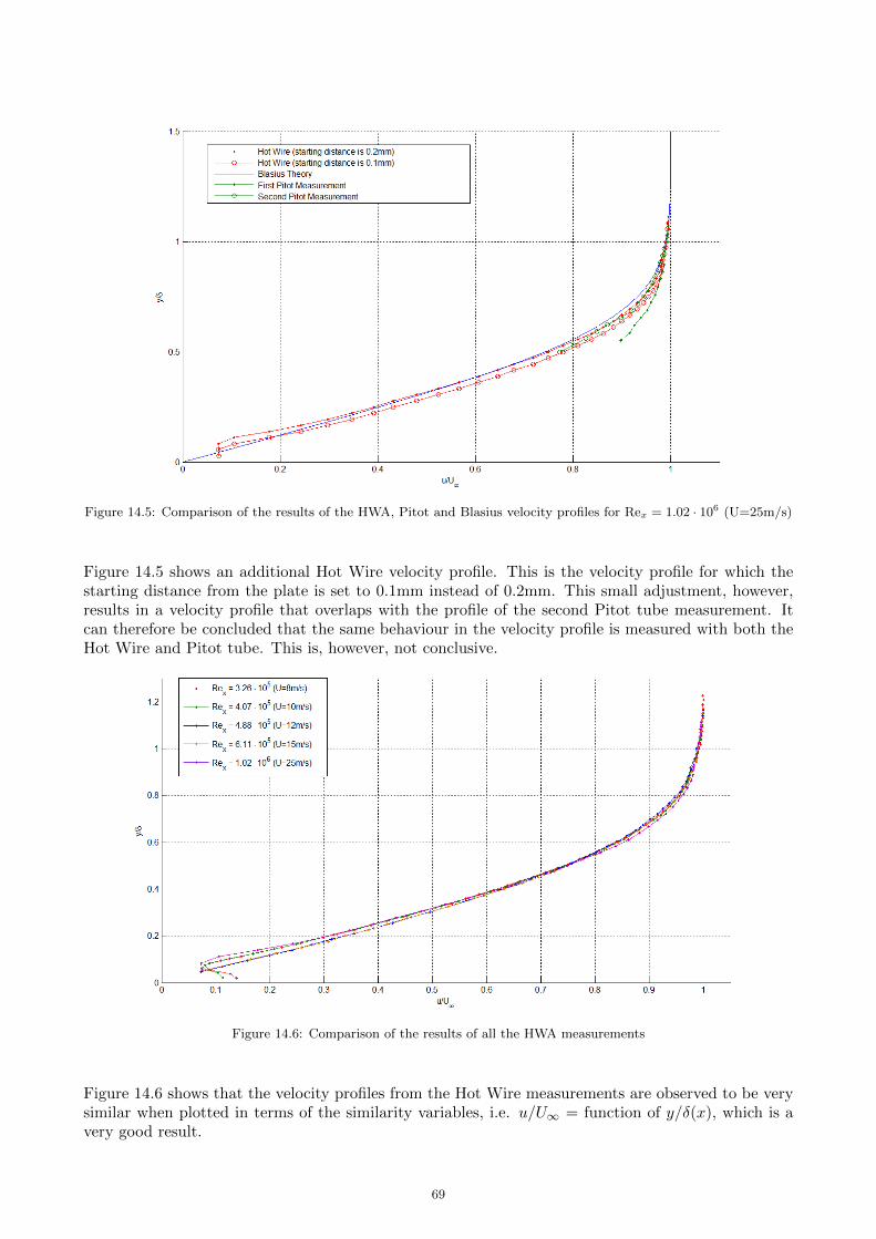
Figure 14.5: Comparison of the results of the HWA, Pitot and Blasius velocity profiles for Rex = 1.02 · 106 (U=25m/s)
Figure 14.5 shows an additional Hot Wire velocity profile. This is the velocity profile for which thestarting distance from the plate is set to 0.1mm instead of 0.2mm. This small adjustment, however,results in a velocity profile that overlaps with the profile of the second Pitot tube measurement. Itcan therefore be concluded that the same behaviour in the velocity profile is measured with both theHot Wire and Pitot tube. This is, however, not conclusive.
Figure 14.6: Comparison of the results of all the HWA measurements
Figure 14.6 shows that the velocity profiles from the Hot Wire measurements are observed to be verysimilar when plotted in terms of the similarity variables, i.e. u/U∞ = function of y/δ(x), which is avery good result.
69
Figure 14.7: Comparison of all the Pitot tube measurements
The comparison of all Pitot tube measurements do not collapse as nicely from the HWA results forthe U=8m/s, U=15m/s and U=25m/s measurements. A follow-up research should investigate if thevariation in the velocity profile relates to anomalies of the surface of the plate as was described insection 13.1.1.
70
15 Discussion
15.1 The Pitot Tube Measurement
If one wants to be more accurate in a measurement with the Pitot tube, some details should betaken into consideration. The pressure difference between the static pressure and stagnation pressureis determined with two different Pitot tubes which are not on the same streamline and Bernoulli’sequation does not hold. Moreover, the static pressure below the plate was found to be not identicalto the static pressure measured with the Pitot tube in the wind tunnel. Therefore a more accuratemethod would be to place the Pitot tubes on the same streamline as much as possible or a Pitot tubeshould be designed which can measure the stagnation and static pressure in the boundary layer.
15.2 The Hot Wire Measurement
In the Hot Wire measurements, the temperature was not logged. However, a temperature changein the flow will have an effect on the voltage which is applied on the HWA. Unfortunately, in thisresearch there was not another opportunity to repeat the measurements and log the temperature.In a follow-up study this should be taken into consideration. Equation 15.1 shows the relation tocompensate for the change in ambient temperature from a reference temperature Ta,r to the actualtemperature Ta which will change the reference voltage Ew,r to Ew. The equation has been obtainedfrom Bruun [8]
Ew = Ew,r
(Tw − TaTw − Ta,r
)1/2
(15.1)
The determination of the distance between the HWA and the plate has also proven to be quite achallenge. We did not have the appropriate tools to determine the distance of the HWA from theplate. The heat transfer from the Hot Wire to the plate also had an influence, specifically close to theplate which can be observed in some of the measurements. However, by referencing the data to theBlasius Theory these effects were minimized.
15.3 The Load Cell Measurement
The drag force measurement gave a very clear picture of the transition from laminar to turbulentflow. However, the temperature of the flow in the wind tunnel affects the measurement of the loadcell and thus the accuracy of the measurement. However, these effects were absolute and did not havean influence on the transition delay. Nonetheless a less temperature sensitive load cell should be usedin future measurements.
71
72
16 Conclusions and Recommendations
16.1 Conclusion
Numerical simulations with XFOIL showed that the designed plate behaves aerodynamically as aninfinitesimally thin flat plate. With a Hot Wire Anemometer and a Pitot tube we were able to measurethe laminar and turbulent velocity profile of the boundary layer on the flat plate. The results showedgreat similarity with the derived theory. The result of the drag force measurement, specifically thevalue of the drag coefficient matched well with the derived theory. However, the measurements canbe performed more accurately if more appropriate methods are used.
The possibility of the presence of disturbances (i.e. turbulent wedges) in the boundary layer at avelocity of U=25m/s (Rex = 1.02 · 106) were observed with the Pitot tube. Furthermore, the result ofthe drag force measurement showed a delayed transition of the flow over the plate in de Silent WindTunnel at Rec ≈ 3 · 106. It was found that the pressure gradient in the test section of the Silent WindTunnel is a possible cause of the transition delay.
16.2 Recommendations
Based on the performed research, a number of recommendations are made for follow-up research.
The measurement with the Pitot tube showed some divergent results compared to the Blasius Theoryand Hot Wire measurement. The discussed difference in stagnation pressure along the span of theplate indicated anomalies in the boundary layer flow. Further research should investigate the devel-opment of disturbances (i.e. turbulent wedges) over the plate in the wind tunnel and the effect of thedisturbances on the measurement.
It should be considered to find a more accurate method to measure the velocity profile with thePitot tube. The used method to calculate the velocity with the stagnation and static pressure wasadequate in this research. Though, a more accurate method to measure the static pressure closer tothe Pitot tube should be reviewed.
During the Hot Wire measurement, it was difficult to determine the exact distance between theHot Wire and the surface of the plate. Accurate methods to determine the exact distance betweenthe Hot Wire and the surface of the plate should be reviewed. A possibility would be to use a laser.Another follow-up study can be considered where one would derive a model for the heat loss of theHot Wire when it gets closer to the surface of the plate.
To investigate the effects of the streamwise pressure gradient on transition, a follow-up research shouldbe conducted in which the plate is installed at a specific angle of attack to change the streamwisepressure gradient. Numerical simulations with XFOIL showed that an angle of attack of 1 ◦ should besufficient to change the streamwise pressure gradient. The effects of the streamwise pressure gradienton transition can then be analyzed. It can also be considered to investigate the origin of the streamwisepressure gradient in the test section of the Silent Wind Tunnel.
The accuracy of the drag force measurement can be increased if a less temperature sensitive loadcell is used, especially for the lower Reynolds number range. It should therefore be considered to useanother load cell for measurements at low Reynolds numbers.
73
74
17 References
1. Dr. R. Hagmeijer, Dictaat ’Inleiding Stromingsleer’, Februari 2013, University of Twente.
2. H.W.M. Hoeijmakers, lecture slide 8, Stromingsleer en Warmteoverdracht, University of Twente,2014.
3. Tuncer Cebeci and Jean Cousteix, ’Modeling and Computation of Boundary-Layer Flow.’, SecondEdition.
4. D. Arnal, G. Casalis and R. Houdeville, ’Practical Transition Prediction Methods: Subsonic andTransonic Flows’, ONERA/DMAE, Toulouse.
5. John D. Anderson Jr., ’Fundamentals of Aerodynamics’, 4th edition, McGraw-Hill InternationalEdition.
6. Jack Chen, ’Journal of Microelectromechanical Systems’ , Vol. 12, No. 6, December 2003.
8. H.H. Bruun, ’Hot-Wire Anemometry: Principles and Signal Analysis’, June 8 1995.
9. Ir. Emiel Koopmans and Jelle Will, ’Turbulence Intensity Measurements of the 130kW SilentWind Tunnel’, December 2013
75
76
Appendix
A The Dimensions of the Plate
The Leading Edge (Hermite Polynomial):
The Trailing Edge (last 70% of NACA 4-series):
77
78
B Matlab Code
clear allclose allclc
%% General Parameters
% Flat plate parametersLE = 'Harry'TE = 'NACA0010';le perc = 0.05;te perc = 0.20;thickness = 0.01;
% Define grid sizenr panels le = 223;nr panels te = 223;nr panels mid = 50;nr panels tot = nr panels le + nr panels te + nr panels mid;% number of points is two times as large.
%% Symbolic curvesyms x;
folder = '01 Nose Harry';airfoil name = ['LE(' LE '-' num2str(le perc) '-R0.2) TE(' TE '-' ...num2str(te perc) ') T(' num2str(thickness) ')'];
P1 = (1+2.0.*x LE temp).*(1.0-x LE temp).*(1.0-x LE temp);P2 = 1.0 - P1;Q1 = x LE temp.*(1.0-x LE temp).*(1.0-x LE temp);Q2 = -x LE temp.*x LE temp.*(1.0-x LE temp);y LE temp = 0.5.*(sqrt(x LE temp).*(b1 + b2.*x LE temp) + df0*Q1 + ...f1*P2 + df1*Q2);
0.1015.*x.ˆ4);diff NACA0010 = diff(NACA0010);maximum = solve(diff NACA0010==0);real maximum = maximum(1);y value maximum = subs(NACA0010,x,real maximum);
x TE temp = (x-(1-te perc/(1-real maximum)))./(te perc/(1-real maximum));y TE temp = 0.05/y value maximum*subs(NACA0010,x,x TE temp);
%% Create one file with all coordinatesx coord upper = zeros(nr panels tot,1);x1 = x values LE';x2 = x values Middle';x3 = x values TE';x coord upper(1:(length(x1)))=x1(1:(length(x1)));x coord upper((length(x1)):(length(x1)+length(x2)-1))=x2(1:length(x2));x coord upper((length(x1)+length(x2)-2):(length(x1)+length(x2)+length(x3)-3))= ...x3(1:length(x3));
y coord upper = zeros((length(x1)+length(x2)+length(x3)-3),1);
for i = 1:length(x coord upper)if x coord upper(i)<le perc
y coord upper(i) = subs(curve LE,x,x coord upper(i));elseif x coord upper(i)>(1-te perc)
y coord upper(i) = subs(curve TE,x,x coord upper(i));else
y coord upper(i) = subs(curve Middle,x,x coord upper(i));end
end
x coord = [flipdim(x coord upper,1); 0; x coord upper];y coord = [-flipdim(y coord upper,1); 0; y coord upper];
Xfoil Airfoil File = [x coord,y coord];%% Check if the maximum number of points in Xfoil is not exceededlength(Xfoil Airfoil File)if length(Xfoil Airfoil File)<1000save('FlatPlate.txt', 'Xfoil Airfoil File', '-ASCII','-append')else
close allerrordlg('Maximum number of points exceeded. Please Reduce','Writing Error');
end
80
C Measurement Apparatus
C.1 The Pitot Tube
Figure C.1 shows the custom made Pitot tube.The tube has a diameter of 3mm. The tip ofthe Pitot tube is located at a distance of approx-imately 620mm from the leading edge. The Pitottube is not located exactly in the middle of thespan of the plate, though this is not expected tohave an effect on the results of the measurement.
Figure C.1: The Pitot tube that was used in the measure-ments
81
C.2 Hot Wire Anemometer
Figure C.2 shows the calibration of the Hot Wire in the Silent Wind Tunnel. The HWA has the sameposition in the tunnel as the Pitot tube. A 1-Dimensional 55P11 Probe from Dantec was used.
Figure C.2: The Hot Wire Anemometer during calibration
C.3 The Streamwise Pressure Gradient Measurement
Figure C.3 shows the position of the pressure orifices in the test section of the Silent Wind Tunnel.Pressure orifice 3 is shown as a lamp in the picture. However, it can be replaced by a pressure gate.
Figure C.3: The pressure gates from which the pressure distribution has been measured in the Silent Wind Tunnel
82
C.4 The Load Cell
Figure C.4 shows the load cell which measures thedrag force. Another load cell is located at theother side of the test section.