Comment. Math. Helv. 72 (1997) 285–315 0010-2571/97/020285-31 $ 1.50+0.20/0 c 1997 Birkh¨auser Verlag, Basel Commentarii Mathematici Helvetici The braid monodromy of plane algebraic curves and hyperplane arrangements Daniel C. Cohen and Alexander I. Suciu * Abstract. To a plane algebraic curve of degree n, Moishezon associated a braid monodromy homomorphism from a finitely generated free group to Artin’s braid group Bn. Using Hansen’s polynomial covering space theory, we give a new interpretation of this construction. Next, we provide an explicit description of the braid monodromy of an arrangement of complex affine hyperplanes, by means of an associated “braided wiring diagram.” The ensuing presentation of the fundamental group of the complement is shown to be Tietze-I equivalent to the Randell- Arvola presentation. Work of Libgober then implies that the complement of a line arrangement is homotopy equivalent to the 2-complex modeled on either of these presentations. Finally, we prove that the braid monodromy of a line arrangement determines the intersection lattice. Examples of Falk then show that the braid monodromy carries more information than the group of the complement, thereby answering a question of Libgober. Mathematics Subject Classification (1991). Primary 14H30, 20F36, 52B30; Secondary 05B35, 32S25, 57M05. Keywords. Braid monodromy, plane curve, hyperplane arrangement, fundamental group, poly- nomial cover, braid group, wiring diagram, intersection lattice. 1. Introduction 1.1. Let C be an algebraic curve in C 2 . In the 1930’s, Zariski commissioned van Kampen to compute the fundamental group of the complement, π 1 (C 2 \C ). The algorithm for doing this was developed in [vK]. Refinements of van Kampen’s algorithm were given by Chisini in the 50’s, and Ch´eniot, Abelson, and Chang in the 70’s. In the early 80’s, Moishezon [Mo] introduced the notion of braid monodromy, which he used to recover van Kampen’s presentation. Finally, Libgober [L1] showed that the * The second author was partially supported by NSF. grant DMS–9504833, and an RSDF grant from Northeastern University.
The braid monodromy of plane algebraic curves andhyperplane arrangements
Daniel C. Cohen and Alexander I. Suciu∗
Abstract. To a plane algebraic curve of degree n, Moishezon associated a braid monodromyhomomorphism from a finitely generated free group to Artin’s braid group Bn. Using Hansen’spolynomial covering space theory, we give a new interpretation of this construction. Next, weprovide an explicit description of the braid monodromy of an arrangement of complex affinehyperplanes, by means of an associated “braided wiring diagram.” The ensuing presentationof the fundamental group of the complement is shown to be Tietze-I equivalent to the Randell-Arvola presentation. Work of Libgober then implies that the complement of a line arrangement ishomotopy equivalent to the 2-complex modeled on either of these presentations. Finally, we provethat the braid monodromy of a line arrangement determines the intersection lattice. Examplesof Falk then show that the braid monodromy carries more information than the group of thecomplement, thereby answering a question of Libgober.
Let C be an algebraic curve in C2. In the 1930’s, Zariski commissioned van Kampento compute the fundamental group of the complement, π1(C2 \ C). The algorithmfor doing this was developed in [vK]. Refinements of van Kampen’s algorithm weregiven by Chisini in the 50’s, and Cheniot, Abelson, and Chang in the 70’s. In theearly 80’s, Moishezon [Mo] introduced the notion of braid monodromy, which heused to recover van Kampen’s presentation. Finally, Libgober [L1] showed that the
∗The second author was partially supported by NSF. grant DMS–9504833, and an RSDFgrant from Northeastern University.
286 D. C. Cohen and A. I. Suciu CMH
2-complex associated to the braid monodromy presentation is homotopy equivalentto C2 \ C.
Let A be an arrangement of hyperplanes in C`. In the early 80’s, Randell[R1] found an algorithm for computing the fundamental group of the complement,π1(C` \ A), when A is the complexification of a real arrangement. Salvetti [S1]subsequently found a regular cell complex that is a deformation retract of the com-plement of such an arrangement. When ` = 2, Falk [Fa] proved that the 2-complexassociated to the Randell presentation is homotopy equivalent to C2 \A by show-ing that it is homotopy equivalent to Salvetti’s complex. The braid monodromy ofa complexified real arrangement was determined by Salvetti [S2], Hironaka [Hir],and Cordovil and Fachada [CF], [Cor]. An algorithm for computing the funda-mental group of an arbitrary complex arrangement was found by Arvola [Ar] (seealso Orlik and Terao [OT], and see Dung and Ha [DH] for another method).
In this paper, we present a unified view of these two subjects, extending severalof the aforementioned results. In particular, we give in 5.3 an algorithm for findingthe (pure) braid monodromy of an arbitrary arrangement A of complex lines inC2. Furthermore, we show in Theorem 6.4 that the corresponding presentation ofπ1(C2 \ A) is equivalent to the Randell-Arvola presentation. We also strengthenFalk’s result, by showing that the 2-complex modeled on the Arvola presentationis homotopy equivalent to C2 \ A.
The determination of the braid monodromy of an arrangement A is facilitat-ed by use of a braided wiring diagram associated to A, a natural generalizationof a combinatorial notion of Goodman [Go]. For a real arrangement, Cordoviland Fachada have shown that the braid monodromy of the complexification isdetermined by an associated (unbraided) wiring diagram, and have defined thebraid monodromy of an abstract wiring diagram. Hironaka’s technique may alsobe applied in this generality. The algorithm presented here generalizes both thesemethods.
1.2.
Before specializing to arrangements, we present a new interpretation of the processby which the braid monodromy of a curve C is defined. This follows in spirit theapproach in [L1], but uses a self-contained argument based on Hansen’s theoryof polynomial covering maps, [H1], [H2]. Given a simple Weierstrass polynomialf : X × C → C of degree n, we consider the space Y = X × C \ {f(x, z) =0}. In Theorem 2.3, we show that the projection p = pr1 |Y : Y → X is afiber bundle map, with structure group the braid group Bn, and monodromy thehomomorphism from π1(X) to Bn induced by the coefficient map of f .
This result is applied in the situation where f defines a plane curve C, andX = C \ {y1, . . . , ys} is the set of regular values of a generic linear projection.The braid monodromy of C is simply the coefficient homomorphism, α : Fs → Bn.This map depends on choices of projection, generating curves, and basepoints.
Vol. 72 (1997) Braid monodromy of curves and arrangements 287
However, the braid-equivalence class of the monodromy—the double coset [α] ∈Bs\Hom(Fs, Bn)/Bn, where Bs acts on the left by the Artin representation, andBn acts on the right by conjugation—is uniquely determined by C.
For a line arrangementA, changes in the various choices noted above give rise tochanges in the associated braided wiring diagram W. These, and other, “Markovmoves” do not affect the braid monodromy. In practice, the braided wiring diagramof a given arrangement may be simplified via these moves. Such simplifications,together with use of the braid relations, make the braid monodromy presentationof the group of a complex arrangement accessible. Furthermore, braided wiringdiagrams associated to arrangements which are lattice-isotopic in the sense ofRandell [R2] are related by Markov moves. A combinatorial characterization ofthis fact remains to be determined. Such a characterization, suggested for (un-braided) wiring diagrams by Bjorner, Las Vergnas, Sturmfels, White, and Zieglerin [BLSWZ], Exercise 6.12, would likely lead to the development of a Jones-typepolynomial for arrangements.
The braid monodromy is also useful in defining Alexander-type invariants ofplane algebraic curves. Given a curve C with braid monodromy α : Fs → Bn,one may consider a representation θ : Bn → GL(N,R), and compute the mod-ule of coinvariants of θ ◦ α. As noted by Libgober in [L3], the R-module Aθ(C) =H0(Fs;RNθ◦α) depends only on the equisingular isotopy class of C (and on θ). Whenθ is the Burau representation, Aθ(C) equals the Alexander module, and thus de-pends only on π1(C2 \ C). For other representations of the braid group, such asthe generalized Burau representations of [CS1], the module Aθ(C) is more likely tobe a homeomorphism-type (rather than homotopy-type) invariant of the comple-ment, see the discussion in 1.3, and section 7. For a detailed analysis of Alexanderinvariants of hyperplane arrangements, based on the techniques developed in thispaper, we refer to [CS2].
1.3.
In general, the braid monodromy of a plane algebraic curve depends not only on thenumber and type of singularities, but on the relative positions of the singularitiesas well. A famous example of Zariski [Z1], [Z2] consists of two sextics, both withsix cusps, one with all cusps on a conic, the other not. Explicit braid monodromygenerators for these curves were given by Rudolph [Ru], Example 3. As shownby Zariski, the two curves have distinct fundamental groups. Further informationconcerning such “Zariski couples” may be found in [A-B]. An example of a differentnature is given in 7.4. There, the two sextics have the same number of doublepoints (9) and triple points (2); their fundamental groups are isomorphic, but,nevertheless, their braid monodromies are not braid-equivalent.
The above example provides an affirmative answer to a question of Libgober,who raised the possibility in [L3] that the braid monodromy of a plane algebraiccurve which is transverse to the line at infinity carries more information than the
288 D. C. Cohen and A. I. Suciu CMH
fundamental group of the complement. The sextics in 7.4 define arrangements,originally studied by Falk [Fa], with distinct lattices. This explains the differencein the braid monodromies: In Theorem 7.2, we show that the braid-equivalenceclass of the monodromy of an arrangement determines the lattice. On the otherhand, as Falk demonstrated with these examples, the homotopy type of the com-plement of an arrangement does not determine the lattice. However, as noted byJiang and Yau [JY], the complements of these arrangements are not homeomor-phic. This, and other evidence, suggests that the braid monodromy of a curve ismore closely tied to the homeomorphism type of the complement (or even to theambient homeomorphism type of the curve) than to the fundamental group of thecomplement.
In the other direction, using classical configurations of MacLane [MacL], Ryb-nikov [Ry] constructs complex arrangements with isomorphic lattices and distinctfundamental groups. It follows that the lattice of a complex arrangement doesnot determine the braid monodromy. We provide another illustration of this phe-nomenon. In Theorem 3.9, we show that complex conjugate algebraic curves haveequivalent braid monodromies. However, we show in 7.7 that the monodromies ofa pair of conjugate arrangements associated to MacLane’s configurations are notbraid-equivalent, despite the fact that these arrangements have isomorphic latticesand groups (and, in fact, diffeomorphic complements).
It is not known whether the lattice of a real arrangement determines the braidmonodromy of its complexification. A result along these lines may be found in[CF]. There, the image in the pure braid group of the braid monodromy of awiring diagram W is called the braid monodromy group of W. Cordovil andFachada show that wiring diagrams which determine identical matroids give rise toequal braid monodromy groups. This result is not as widely applicable as it mayappear. In 7.5, we consider arrangements with isomorphic (oriented) matroidsand homeomorphic complements. Their monodromies are braid-equivalent, butthe associated braid monodromy groups are not conjugate subgroups of the purebraid group.
Conventions. Given elements x and y in a group G, we will write xy = y−1xyand [x, y] = xyx−1y−1. Also, we will denote by Aut(G) the group of right auto-morphisms of G, with multiplication α · β = β ◦ α.
Acknowledgements
We would like to thank Mike Falk for useful conversations, and for sharing withus his unpublished work with Bernd Sturmfels, as well as that of John Keaty.
Vol. 72 (1997) Braid monodromy of curves and arrangements 289
2. Polynomial covers and Bn-bundles
We begin by reviewing polynomial covering maps. These were introduced byHansen in [H1], and studied in detail in his book [H2], which, together with Bir-man’s book [Bi], is our basic reference for this section. We then consider bundleswhose structure group is Artin’s braid group Bn, and relate them to polynomialn-fold covers.
2.1. Polynomial covers
Let X be a path-connected space that has the homotopy type of a CW-complex.A simple Weierstrass polynomial of degree n is a map f : X × C→ C given by
f(x, z) = zn +n∑i=1
ai(x)zn−i,
with continuous coefficient maps ai : X → C, and with no multiple roots forany x ∈ X . Given such f , the restriction of the first-coordinate projection mappr1 : X × C→ X to the subspace
E = E(f) = {(x, z) ∈ X × C | f(x, z) = 0}
defines an n-fold cover π = πf : E → X , the polynomial covering map associatedto f .
Since f has no multiple roots, the coefficient map a = (a1, . . . , an) : X → Cntakes values in the complement of the discriminant set, Bn = Cn \∆n. Over Bn,there is a canonical n-fold polynomial covering map πn = π
fn: E(fn) → Bn,
determined by the Weierstrass polynomial fn(x, z) = zn +∑ni=1 xiz
n−i. Clearly,the polynomial cover πf : E(f) → X is the pull-back of πn : E(fn) → Bn alongthe coefficient map a : X → Bn.
This can be interpreted on the level of fundamental groups as follows. Thefundamental group of the configuration space, Bn, of n unordered points in Cis the group, Bn, of braids on n strands. The map a determines the coefficienthomomorphism α = a∗ : π1(X)→ Bn, unique up to conjugacy. One may charac-terize polynomial covers as those covers π : E → X for which the characteristichomomorphism to the symmetric group, χ : π1(X) → Σn, factors through thecanonical surjection τn : Bn → Σn as χ = τn ◦ α.
Now assume that the simple Weierstrass polynomial f is completely solvable,that is, factors as
f(x, z) =n∏i=1
(z − bi(x)),
with continuous roots bi : X → C. Since the Weierstrass polynomial f is sim-ple, the root map b = (b1, . . . , bn) : X → Cn takes values in the complement,
290 D. C. Cohen and A. I. Suciu CMH
Pn = Cn \ An, of the braid arrangement An = {ker(wi − wj)}1≤i<j≤n. Over Pn,there is a canonical n-fold covering map, qn = πQn : E(Qn)→ Pn, determined bythe Weierstrass polynomial Qn(w, z) = (z −w1) · · · (z −wn). Evidently, the coverπf : E → X is the pull-back of qn : E(Qn)→ Pn along the root map b : X → Pn.
The fundamental group of the configuration space, Pn, of n ordered points inC is the group, Pn = ker τn, of pure braids on n strands. The map b determinesthe root homomorphism β = b∗ : π1(X) → Pn, unique up to conjugacy. Thepolynomial covers which are trivial covers (in the usual sense) are precisely thosefor which the coefficient homomorphism factors as α = ιn ◦β, where ιn : Pn → Bnis the canonical injection.
2.2. Bn-Bundles
The group Bn may be realized as the mapping class group Mn0,1 of orientation-
preserving diffeomorphisms of the disk D2, permuting a collection of n markedpoints. Upon identifying π1(D2 \ {n points}) with the free group Fn, the actionof Bn on π1 yields the Artin representation, αn : Bn → Aut(Fn). As shown byArtin, this representation is faithful. Hence, we may—and often will—identify abraid θ ∈ Bn with the corresponding braid automorphism, αn(θ) ∈ Aut(Fn).
Now let f : X×C→ C be a simple Weierstrass polynomial. Let πf : E(f)→ Xbe the corresponding polynomial n-fold cover, and a : X → Bn the coefficient map.Consider the complement
Y = Y (f) = X × C \E(f),
and let p = pf : Y (f)→ X be the restriction of pr1 : X × C→ X to Y .
Theorem 2.3. The map p : Y → X is a locally trivial bundle, with structuregroup Bn and fiber Cn = C \ {n points}. Upon identifying π1(Cn) with Fn, themonodromy of this bundle may be written as αn ◦ α, where α = a∗ : π1(X)→ Bnis the coefficient homomorphism.
Moreover, if f is completely solvable, the structure group reduces to Pn, andthe monodromy factors as αn ◦ ιn ◦ β, where β = b∗ : π1(X) → Pn is the roothomomorphism.
Proof. We first prove the theorem for the configuration spaces, and their canonicalWeierstrass polynomials. Start with X = Pn, f = Qn, and the canonical coverqn : E(Qn) → Pn. Clearly, Y (Qn) = Cn+1 \ E(Qn) is equal to the configurationspace Pn+1. Let ρn = p
Qn: Pn+1 → Pn be the restriction of pr1 : Cn ×C→ Cn.
As shown by Fadell and Neuwirth [FN], this is a bundle map, with fiber Cn, andmonodromy the restriction of the Artin representation to Pn.
Next, consider X = Bn, f = fn, and the canonical cover πn : E(fn) →Bn. Forgetting the order of the points defines a covering projection from theordered to the unordered configuration space, κn : Pn → Bn. In coordinates,
Vol. 72 (1997) Braid monodromy of curves and arrangements 291
κn(w1, . . . , wn) = (x1, . . . , xn), where xi = (−1)isi(w1, . . . , wn), and si are theelementary symmetric functions. By Vieta’s formulas, we have
Qn(w, z) = fn(κn(w), z).
Let Y n+1 = Y (fn) and pn = pfn : Y n+1 → Bn. By the above formula, we seethat κn× id : Pn×C→ Bn×C restricts to a map κn+1 : Y (Qn)→ Y (fn), whichfits into the fiber product diagram
Pn+1 ρn−−−−→ Pnyκn+1
yκnY n+1 pn
−−−−→ Bn
where the vertical maps are principal Σn-bundles. Since the bundle map ρn :Pn+1 → Pn is equivariant with respect to the Σn-actions, the map on quotients,pn : Y n+1 → Bn, is also a bundle map, with fiber Cn, and monodromy action theArtin representation of Bn. This finishes the proof in the case of the canonicalWeierstrass polynomials over configuration spaces.
Now let f : X × C → C be an arbitrary simple Weierstrass polynomial. Wethen have the following cartesian square:
Y −−−−→ Y n+1yp ypnX
a−−−−→ Bn
In other words, p : Y → X is the pullback of the bundle pn : Y n+1 → Bn alongthe coefficient map a. Thus, p is a bundle map, with fiber Cn, and monodromyrepresentation αn ◦ α. When f is completely solvable, the bundle p : Y → X isthe pullback of ρn : Pn+1 → Pn along the root map b. Since α = ιn ◦ β, themonodromy is as claimed. �
Remark 2.4. Let us summarize the above discussion of braid bundles over con-figuration spaces. From the Fadell-Neuwirth theorem, it follows that Pn is aK(Pn, 1) space. Since the pure braid group is discrete, the classifying Pn-bundle(in the sense of Steenrod) is the universal cover Pn → Pn. We considered twobundles over Pn, both associated to this one:(i) qn : E(Qn)→ Xn, by the trivial representation of Pn on {1, . . . , n};(ii) ρn : Pn+1 → Pn, by the (geometric) Artin representation of Pn on Cn.Since Bn is covered by Pn, it is a K(Bn, 1) space, and the classifying Bn-bundleis Bn → Bn. There were three bundles over Bn that we mentioned, all associatedto this one:
292 D. C. Cohen and A. I. Suciu CMH
(iii) κn : Xn → Bn, by the canonical surjection τn : Bn → Σn;(iv) πn : E(fn)→ Bn, by the above, followed by the permutation representation of
Σn on {1, . . . , n};(v) pn : Y n+1 → Bn, by the (geometric) Artin representation of Bn on Cn.Finally, note that π1(Y n+1) is isomorphic to B1
n = FnoαnBn, the group of braidson n + 1 strands that fix the endpoint of the last strand, and that Y n+1 is aK(B1
n, 1) space.
3. The braid monodromy of a plane algebraic curve
We are now ready to define the braid monodromy of an algebraic curve in thecomplex plane. The construction, based on classical work of Zariski and van Kam-pen, is due to Moishezon [Mo]. We follow the exposition of Libgober [L1], [L2],[L3], but interpret the construction in the context established in the previous sec-tion.
3.1. The construction
Let C be a reduced algebraic curve in C2, with defining polynomial f of degreen. Let π : C2 → C be a linear projection, and let Y = {y1, . . . , ys} be the set ofpoints in C for which the fibers of π contain singular points of C, or are tangentto C. Assume that π is generic with respect to C. That is, for each k, the lineLk = π−1(yk) contains at most one singular point vk of C, and does not belongto the tangent cone of C at vk, and, moreover, all tangencies are simple. Let Ldenote the union of the lines Lk, and let y0 be a basepoint in C\Y. The definitionof the braid monodromy of C depends on two observations:
(i) The restriction of the projection map, p : C2 \C ∪L → C\Y, is a locally trivialbundle.
Fix the fiber Cn = p−1(y0) and a basepoint y0 ∈ Cn. The monodromy of C is,by definition, the holonomy of this bundle, ρ : π1(C \ Y, y0) → Aut(π1(Cn, y0)).Upon identifying π1(C\Y, y0) with Fs, and π1(Cn, y0) with Fn, this can be writtenas ρ : Fs → Aut(Fn).
(ii) The image of ρ is contained in the braid group Bn (viewed as a subgroup ofAut(Fn) via the Artin embedding αn).
The braid monodromy of C is the homomorphism α : Fs → Bn determined byαn ◦ α = ρ.
We shall present a self-contained proof of these two assertions, and, in theprocess, identify the map α. The first assertion is well-known, and can also be
Vol. 72 (1997) Braid monodromy of curves and arrangements 293
proved by standard techniques (using blow-ups and Ehresmann’s criterion—see[Di], page 123), but we find our approach sheds some light on the underlyingtopology of the situation.
3.2. Braid monodromy and polynomial covers
Let π : C2 → C1 be a linear projection, generic with respect to the given algebraiccurve C of degree n. We may assume (after a linear change of variables in C2
if necessary) that π = pr1, the projection map onto the first coordinate. In thechosen coordinates, the defining polynomial f of C may be written as f(x, z) =zn +
∑ni=1 ai(x)zn−i. Since C is reduced, for each x /∈ Y, the equation f(x, z) = 0
has n distinct roots. Thus, f is a simple Weierstrass polynomial over C \ Y, and
π = πf : C \ C ∩ L → C \ Y (1)
is the associated polynomial n-fold cover.Note that Y (f) = ((C \ Y) × C) \ (C \ C ∩ L) = C2 \ C ∪ L. By Theorem 2.3,
the restriction of pr1 to Y (f),
p : C2 \ C ∪ L → C \ Y, (2)
is a bundle map, with structure group Bn, fiber Cn, and monodromy homomor-phism
α = a∗ : π1(C \ Y)→ Bn. (3)
This proves assertions (i) and (ii). Furthermore, we have
Theorem 3.3. The braid monodromy of a plane algebraic curve coincides withthe coefficient homomorphism of the associated polynomial cover.
In the case where C = A is an arrangement of (affine) lines in C2, more can besaid. First, the critical set Y = {y1, . . . , ys} consists (only) of the images underπ = pr1 of the vertices of the arrangement. Furthermore, a defining polynomialfor A can be written as f(x, z) =
∏ni=1(z − `i(x)), where each `i is a linear
function in x. Thus, the associated polynomial cover is trivial, and the monodromyrepresentation is
λ = `∗ : π1(C \ Y)→ Pn.
An explicit formula for λ will be given in section 5. For now, let us record thefollowing:
Theorem 3.4. The pure braid monodromy of a line arrangement coincides withthe root homomorphism of the associated (trivial) polynomial cover.
294 D. C. Cohen and A. I. Suciu CMH
3.5. Braid equivalence
The braid monodromy of a plane algebraic curve is not unique, but rather, dependson the choices made in defining it. This indeterminacy was studied by Libgoberin [L2], [L3]. To make the analysis more precise, we first need a definition.
Definition 3.6. Two homomorphisms α : Fs → Bn and α′ : Fs → Bn are equiva-lent if there exist automorphisms ψ ∈ Aut(Fs) and φ ∈ Aut(Fn) with φ(Bn) ⊂ Bnsuch that α′(ψ(g)) = φ−1 · α(g) · φ, for all g ∈ Fs. In other words, the followingdiagram commutes
Fsα
−−−−→ Bnyψ yconjφ
Fsα′
−−−−→ Bn
If, moreover, ψ ∈ Bs and φ ∈ Bn, the homomorphisms α and α′ are braid-equivalent.
Theorem 3.7. The braid monodromy of a plane algebraic curve C is well-definedup to braid-equivalence.
Proof. First fix the generic projection. The identification π1(C \ Y) = Fs dependson the choice of a “well-ordered” system of generators (see [Mo] or the discussionin 4.1), and any two such choices yield monodromies which differ by a braid auto-morphism of Fs, see [L2]. Furthermore, there is the choice of basepoints, and anytwo such choices yield monodromies differing by a conjugation in Bn.
Finally, one must analyze the effect of a change in the choice of generic projec-tion. Let π and π′ be two such projections, with critical sets Y and Y ′, and braidmonodromies α : π1(C \ Y)→ Bn and α′ : π1(C \ Y ′)→ Bn. Libgober [L3] showsthat there is a homeomorphism h : C → C, isotopic to the identity, and takingY to Y ′, for which the isomorphism h∗ : π1(C \ Y) → π1(C \ Y ′) induced by therestriction of h satisfies α′ ◦ h∗ = α. From the construction, we see that h can betaken to be the identity outside a ball of large radius (containing Y ∪ Y ′). Thus,once the identifications of source and target with Fs are made, h∗ can be written asthe composite of an inner automorphism of Fs with a braid automorphism of Fs:h∗ = conjg ◦ψ. Trading the inner automorphism of Fs for an inner automorphismof Bn, we obtain α′ ◦ ψ = conjα′(g) ◦α, completing the proof. �
Thus, we may regard the braid monodromy of C as a braid-equivalence class,i.e., as a double coset [α] ∈ Bs\Hom(Fs, Bn)/Bn, uniquely determined by C. Infact, it follows from [L3] that [α] depends only on the equisingular isotopy class ofthe curve.
Vol. 72 (1997) Braid monodromy of curves and arrangements 295
3.8. Conjugate curves
If C is a plane curve with defining polynomial f = f(x, z) of degree n, let C be thecurve defined by the polynomial f whose coefficients are the complex conjugates ofthose of f . In other words, f(x, z) = f(x, z). In this subsection, we relate the braidmonodromies of C and C. In general, the braid monodromies of conjugate curvesare not braid-equivalent, as shown in 7.7. Nevertheless, we have the following:
Theorem 3.9. The braid monodromies of conjugate curves are equivalent.
Proof. Let C and C be conjugate curves defined by polynomials f and f of degreen. Choose coordinates in C2 so that π = pr1 is generic with respect to C. Thenπ is evidently also generic with respect to C. Let Y and Y be the critical sets ofC and C with respect to this projection. Complex conjugation C → C restrictsto a map d : C \ Y → C \ Y. Choose a basepoint y0 with Im(y0) = 0. Thend induces an isomorphism d∗ : π1(C \ Y, y0) → π1(C \ Y, y0). Identifying thesegroups with Fs = 〈x1, . . . , xs〉, we have d∗ = δs, where δs ∈ Aut(Fs) is given byδs(xk) = (x1 · · ·xk−1) · x−1
k · (x1 · · ·xk−1)−1.Since the discriminant locus ∆n is defined by a polynomial with real coefficients,
complex conjugation Cn → Cn restricts to a map e : Bn → Bn. The induced mapεn = e∗ : Bn → Bn is readily seen to be the automorphism defined on generatorsby εn(σi) = σ−1
i . As shown by Dyer and Grossman [DG], this involution generatesOut(Bn) = Z2, for n ≥ 3.
Let a and a be the coefficient maps of f and f respectively. The fact thatthe defining polynomials of C and C have complex conjugate coefficients may beexpressed as a ◦ d = e ◦ a. Passing to fundamental groups, we have α ◦ δs = εn ◦α.Checking that εn = conjδn (see [DG]) completes the proof. �
4. The fundamental group of a plane algebraic curve
We now give the braid monodromy presentation of the fundamental group of thecomplement of a plane algebraic curve C. This presentation first appeared in theclassical work of van Kampen and Zariski [vK], [Z2], and has been much studiedsince, see e.g. [Mo], [MT], [L1], [L2], [Ru], [Di].
4.1. Braid monodromy presentation
The homotopy exact sequence of the bundle p : C2 \ C ∪ L → C \ Y of (2) reducesto
1→ π1(Cn)→ π1(C2 \ C ∪ L)p∗−→ π1(C \ Y)→ 1.
This sequence is split exact, with action given by the braid monodromy homo-
296 D. C. Cohen and A. I. Suciu CMH
morphism α of (3). To extract a presentation of the middle group, order thepoints of Y by decreasing real part, and pick the basepoint y0 in C \ Y withRe(y0) > max{Re(yk)}. Choose loops ξk : [0, 1] → C \ Y based at y0, goingup and above y1, . . . , yk−1, passing around yk in the counterclockwise direction,and coming back the same way. Setting xk = [ξk], identify π1(C \ Y, y0) withFs = 〈x1, . . . , xs〉. Similarly, identify π1(Cn, y0) with Fn = 〈t1, . . . , tn〉. Hav-ing done this, π1(C2 \ C ∪ L, y0) becomes identified with the semidirect productFn oα Fs. The corresponding presentation is
The fundamental group of the complement of the curve is the quotient ofπ1(C2 \ C ∪ L) by the normal closure of Fs = 〈x1, . . . , xs〉. Thus, π1(C2 \ C) =〈t1, . . . , tn | ti = α(xk)(ti)〉. This presentation can be simplified by Tietze-IImoves—eliminating redundant relations. Doing so, one obtains the braid mon-odromy presentation
π1(C2 \ C) = 〈t1, . . . , tn | ti = α(xk)(ti), i = j1, . . . , jmk−1; k = 1, . . . , s〉. (4)
If yk corresponds to a singular point of C, then mk denotes the multiplicity of thatsingular point, while if yk corresponds to a (simple) tangency point, mk = 2. Ineither case, the indices j1, . . . , jmk−1 must be chosen appropriately, see [L1] andthe discussions in 5.1 and 6.1.
Let K(C) be the 2-complex modeled on the braid monodromy presentation.There is an obvious embedding of this complex into the complement of C. Themain result of [L1] is the following.
Theorem 4.2. (Libgober) The 2-complex K(C) is a deformation retract of C2\C.
Remark 4.3. The group G(α) defined by presentation (4) is the quotient ofFn by the normal subgroup generated by {γ(t) · t−1 | γ ∈ im(α), t ∈ Fn}. Inother words, G(α) is the maximal quotient of Fn on which the representationα : Fs → Bn acts trivially. If α′ : Fs → Bn is equivalent to α, then G(α) isisomorphic to G(α′). Indeed, the equivalence condition α′ ◦ ψ = conjφ ◦α can bewritten as φ(α(g)(t) · t−1) = α′(ψ(g))(φ(t)) · φ(t)−1, ∀g ∈ Fs, ∀t ∈ Fn. Thusφ ∈ Aut(Fn) induces an isomorphism φ : G(α)→ G(α′).
4.4. Braid monodromy generators
We now make the presentation (4) more precise. First recall that the braid groupBn has generators σ1, . . . , σn−1, and relations σiσi+1σi = σi+1σiσi+1 (1 ≤ i <n − 1), σiσj = σjσi (|i − j| > 1), see [Bi], [H2]. The Artin representation αn :
Vol. 72 (1997) Braid monodromy of curves and arrangements 297
Bn → Aut(Fn) is given by:
σi(tj) =
titi+1t
−1i if j = i,
ti if j = i+ 1,tj otherwise.
For each k = 1, . . . , s, let γk ∈ Bmk < Bn be the “local monodromy” aroundyk. Then
α(xk) = β−1k γkβk,
where βk ∈ Bn is the monodromy along the portion of ξk from y0 to just beforeyk. One would like to express these braids in terms of the standard generators σiof Bn. This may be accomplished in two steps.
Step 1. The structure of the (isolated) singularity vk above yk determines thelocal braid γk. This braid may be obtained from the Puiseux series expansion ofthe defining polynomial f(x, z) of C. This is implicit in the work of Brieskorn andKnorrer [BK] and Eisenbud and Neumann [EN].
Example 4.5. Consider the plane curve C : zp−xq = 0. The fundamental groupof its complement was determined by Oka [Ok]. A look at Oka’s computationreveals that the braid monodromy generator is (σ1 · · ·σp−1)q ∈ Bp. For instance,to a simple tangency corresponds σ1, to a node, σ2
1 , and to a cusp, σ31 .
Example 4.6. By the above, the braid monodromy generator of a central linearrangementA : zn−xn = 0 is a full twist on n strands, ∆2 = (σ1 · · ·σn−1)n ∈ Bn(see also [Hir]).
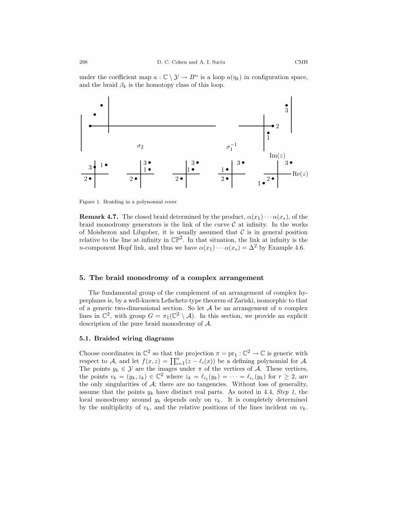
Step 2. The conjugating braids βk depend on the relative positions of the singu-larities of C. These braids may be specified as follows. Let ηk denote the portionof the path ξk from y0 to just before yk. The braid βk is identified by trackingthe components of the fiber of the polynomial cover π = πf : C \ C ∩ L → C \ Yof (1) over ηk. Generically, these components have distinct real parts. Braidingoccurs when the real parts of two components coincide. We record this braidingby analyzing the imaginary parts of the components, as indicated in the figurebelow.
More explicitly, recall that the polynomial cover π is embedded in the trivialline bundle pr1 : (C \ Y) × C → C \ Y. Let y′k = yk + ε denote the endpoint ofthe path ηk. Without loss of generality, we may assume that the components ofπ−1(y′k) (resp. π−1(y0)) have distinct real parts. After an isotopy of C, we mayassume further that the positions of the components of π−1(y′k) in pr−1
1 (y′k) = Care identical to those of π−1(y0) in pr−1
1 (y0) = C. Then the image of the path ηk
298 D. C. Cohen and A. I. Suciu CMH
under the coefficient map a : C \ Y → Bn is a loop a(ηk) in configuration space,and the braid βk is the homotopy class of this loop.
Remark 4.7. The closed braid determined by the product, α(x1) · · ·α(xs), of thebraid monodromy generators is the link of the curve C at infinity. In the worksof Moishezon and Libgober, it is usually assumed that C is in general positionrelative to the line at infinity in CP2. In that situation, the link at infinity is then-component Hopf link, and thus we have α(x1) · · ·α(xs) = ∆2 by Example 4.6.
5. The braid monodromy of a complex arrangement
The fundamental group of the complement of an arrangement of complex hy-perplanes is, by a well-known Lefschetz-type theorem of Zariski, isomorphic to thatof a generic two-dimensional section. So let A be an arrangement of n complexlines in C2, with group G = π1(C2 \ A). In this section, we provide an explicitdescription of the pure braid monodromy of A.
5.1. Braided wiring diagrams
Choose coordinates in C2 so that the projection π = pr1 : C2 → C is generic withrespect to A, and let f(x, z) =
∏ni=1(z − `i(x)) be a defining polynomial for A.
The points yk ∈ Y are the images under π of the vertices of A. These vertices,the points vk = (yk, zk) ∈ C2 where zk = `i1(yk) = · · · = `ir (yk) for r ≥ 2, arethe only singularities of A; there are no tangencies. Without loss of generality,assume that the points yk have distinct real parts. As noted in 4.4, Step 1, thelocal monodromy around yk depends only on vk. It is completely determinedby the multiplicity of vk, and the relative positions of the lines incident on vk.
Vol. 72 (1997) Braid monodromy of curves and arrangements 299
These data, and the braiding of the lines of A over the paths ηk, determine thebraid monodromy of the arrangement. All of this information may be effectivelyrecorded as follows.
Order the points of Y as before, and choose the basepoint y0 ∈ C \ Y so thatRe(y0) > Re(y1) > · · · > Re(ys). Let ξ : [0, 1]→ C be a (smooth) path emanatingfrom y0 and passing through y1, . . . , ys in order. Note that we may take the pathξ to be a horizontal line segment in a neighborhood of each yk. Call such a pathadmissible. Let
W = {(x, z) ∈ ξ × C | f(x, z) = 0}be the braided wiring diagram associated to A. Note that W depends on thegeneric linear projection π and on the admissible path ξ. If {z = `i(x)} is a line ofA, we call W ∩ {z = `i(x)} the associated wire. Since the path ξ passes throughthe points of Y, the vertices of A are contained in W.
Over portions of the path ξ between the points of Y, the lines of A (resp. wiresof W) may braid. Let y′k = yk + ε, and y′′k = yk − ε, for some sufficiently small ε.We may assume that, over y′k and y′′k , the wires of W (i.e., the components of thefiber of the polynomial cover πf ) have distinct real parts. Arguing as in 4.4, Step2, we associate a braid βk,k+1 to the portion of ξ from y′′k to y′k+1.
After an isotopy of A, we may also assume that the positions of the wires ofW over the points y0, y′k, and y′′k are all identical. Thus a braided wiring diagramW may be abstractly specified by a sequence of states, vertices, and braids:
Πs+1βs,s+1←−−−−−
Vs←− Πs ←−←− · · · ←−←− Π2β1,2←−−−
V1←− Π1β0,1←−−− Π0,
where the states Πk are permutations of {1, . . . , n} beginning with the identitypermutation and recording the relative heights of the wires. The vertex set Vk ={i1, . . . , ir} records the indices of the wires incident on the kth vertex vk of A (interms of the order given by the initial state Π0). The braids βk,k+1 are obtainedas above. By choosing the basepoint y0 sufficiently close to y1, we may assumethat the initial braid β0,1 is trivial. If such a diagram is depicted as above, thebraids βk,k+1 should be read off from left to right. Note that the this notiongeneralizes that of a wiring diagram due to Goodman [Go], and that the admissible2-graphs utilized by Arvola [Ar], [OT], may be viewed as examples of braidedwiring diagrams. Explicit examples are given in section 7.
5.2. Generators of Pn
Before proceeding, we need to review some facts about the pure braid group Pn =ker(τn : Bn → Σn). This group has generators
Ai,j = σj−1 · · ·σi+1 · σ2i · σ−1
i+1 · · ·σ−1j−1, 1 ≤ i < j ≤ n,
and relations that set a generator equal to a certain conjugate of itself, see [Bi],[Ha]. In particular, H1(Pn) = Z(n2) is generated by the images of the generators
300 D. C. Cohen and A. I. Suciu CMH
Ai,j . The conjugation action of Bn on Pn is given by the following formulas(compare [DG]):
Aσki,j =
Ai−1,j if k = i− 1,
AAi,i+1i+1,j if k = i < j − 1,
Ai,j−1 if k = j − 1 > i,
AAj,j+1i,j+1 if k = j,
Ai,j otherwise,
Aσ−1ki,j =
AA−1i−1,i
i−1,j if k = i− 1,Ai+1,j if k = i < j − 1,
AA−1j−1,j
i,j−1 if k = j − 1 > i,Ai,j+1 if k = j,Ai,j otherwise.
(5)We shall work mainly with a particular type of pure braids. These “twist
braids” are defined as follows. Given an increasingly ordered set I = {i1, . . . , ir},let
We extend this definition to sets which are not increasingly ordered (such as thevertex sets Vk in 5.1) by first ordering, then proceeding as above. The conjugationaction of an arbitrary braid β ∈ Bn on the twist braid AI ∈ Pn takes the form
AβI = ACω(I), (7)
where ω = τn(β), and C = C(I, β) is a pure braid that may be computed recur-sively from (5).
5.3. Braid monodromy
We now extract the braid monodromy of A from an associated braided wiringdiagram W. By Theorem 3.4, the image of the braid monodromy is containedin the pure braid group Pn. We shall express the braid monodromy generators,λk := λ(xk), in terms of the standard generators Ai,j .
The vertex set Vk = {i1, . . . , ir} gives rise to a partition Πk = Lk ∪ Vk ∪ Uk,where Lk (resp. Uk) consists of the indices of the wires below (resp. above) thevertex vk. Let Ik = {j, j + 1, . . . , j + r − 1} denote the local index of Vk, wherej = |Lk|+ 1. The local monodromy γk around the point yk ∈ Y is a full twist onIk given by the pure braid AIk (compare 4.6). Note that AIk = µ2
is a permutation braid—a half twist on Ik. Also notice that the monodromy alonga path from y′k to y′′k above (or below) the point yk is given by µIk .
To specify the braid monodromy of A, it remains to identify the conjugatingbraids βk of 4.4, Step 2. Choosing the paths ηk to coincide with ξ between y′′j andy′j+1 for j < k, these conjugating braids may be expressed as β1 = β0,1 = 1, and
Vol. 72 (1997) Braid monodromy of curves and arrangements 301
βk+1 = βk,k+1 · µIk · βk for k ≥ 1. Hence the braid monodromy generators aregiven by
λk = AβkIk . (9)
Note that the state Πk of the braided wiring diagram W is the image of thebraid βk in the symmetric group, Πk = τn(βk). Note also that the vertex set Vkand its local index Ik are related by Vk = Πk(Ik). Thus, the braid monodromygenerators may be expressed solely in terms of pure braids:
λk = ACkVk , (10)
for certain Ck ∈ Pn.
5.4. Conjugate arrangements
Let A be an arrangement of n lines in C2, with associated braided wiring diagramW corresponding to a generic projection π : C2 → C and admissible path ξ. LetA denote the conjugate arrangement (see 3.8). Clearly, the vertices of A are thecomplex conjugates of those of A. Thus, π is generic with respect to A, and ξ isadmissible. The corresponding braided diagram, W, is then obtained from W bysimply reversing the crossings of all the intermediate braids. Thus, the local indicesof W are given by Ik = Ik, the conjugating braids by βk+1 = εn(βk,k+1) · µIk · βk,and the braid monodromy generators by λk = AβkIk . From the proof of Theorem 3.9,we see that the braid monodromy generators of the two conjugate arrangementsare related by
λk = εn(
(λ−1k )λ
−1k−1···λ
−11).
5.5. Real arrangements
If A is a real arrangement in C2 (that is, A is the complexification of a linearrangement AR in R2), then the defining polynomial f(x, z) has real coefficients.Consequently, the vertices of A all have real coordinates, and their images underfirst-coordinate projection all lie on the real axis in C. In this instance, we maytake the path ξ : [0, 1] → C to be a directed line segment along the real axis.The resulting diagram W is unbraided—all the intermediate braids βk,k+1 aretrivial. In other words, the diagram is a wiring diagram in the combinatorial sense[Go], affine if A contains parallel lines (see also [BLSWZ]). In this instance, thedescription of the braid monodromy given in 5.3 specializes to the algorithm ofHironaka [Hir], modulo some notational differences.
Another description of the braid monodromy of an abstract (unbraided) wiringdiagram was provided by Cordovil and Fachada in [CF] (see also [Cor]). Thisdescription, based on Salvetti’s work [S1], [S2], may be paraphrased as follows.
Recall that the vertex set Vk = {i1, . . . , ir} gives rise to a partition Πk =Lk ∪ Vk ∪ Uk. Let Vk = {i | i1 ≤ i ≤ ir}, and set Jk = (Vk \ Vk) ∩ Uk. Let
302 D. C. Cohen and A. I. Suciu CMH
BJk =∏Aj,i, where the product is over all j ∈ Jk and i ∈ Vk with j < i,
taken in the natural order (so that BJk is a subword of ∆2 = A1,...,n, equalto 1 if Jk = ∅). Then the braid monodromy generators may be expressed asλk = AJkVk := B−1
JkAVkBJk , where AVk is as defined in (6).
Using the Artin representation, one can show that the braids λk and λk areequal. The action of the braid λk is given in formulas (12) and (13) in section 6.The same formulas hold for λk, but the computation is more involved. Thus, thetwo descriptions of the braid monodromy of a real arrangement (or more generally,of an arbitrary wiring diagram) coincide.
5.6. Markov moves
For an arbitrary complex arrangement A, changes in the choices made in theconstruction of the braid monodromy (see 3.5) give rise to changes in the braidedwiring diagram W associated to A. For instance, changing the basepoint y0 mayalter the initial braid β0,1, while changes in the generic projection may alter theorder of the vertices.
We refer to these (and other) changes in a braided wiring diagram as “Markovmoves.” In practice, these moves may be used to simplify a braided wiring di-agram associated to an arrangement A (and consequently the braid monodromygenerators of A as well). We now record these simplifying Markov moves and theireffects on the braid monodromy. In the following, we record only the local index ofa vertex, so “vertex {j, . . . , k}” means “a vertex with local index {j, . . . , k}.” Re-call that, while we depict braided wiring diagrams right to left, their intermediatebraids are read left to right.
Geometric moves.(1) Insert an arbitrary braid β0 at the beginning of the braided wiring diagram.(2) Insert an arbitrary braid βs+1 at the end of the braided wiring diagram.(3) Replace vertex {i, . . . , j}, then vertex {k, . . . , l} with
(a) vertex {k, . . . , l}, then vertex {i, . . . , j}, if j < k or i > l.(b) braid (σk · · ·σi+1) · (σk+1 · · ·σi+2) · · · (σl−1 · · ·σj),
then vertex {i, . . . , i+ l − k}, then vertex {i+ l − k, . . . , l},then braid (σ−1
Figure 3. Moves 5b (left), 5c (right), and 5d (bottom)
The parity of the braids in move (3) and move (5) may be switched. Forinstance, one can replace braid σ−1
i , then vertex {j, . . . , k}, with braid σj · · ·σk−1,then vertex {j + 1, . . . , k + 1}, then braid σ−1
k · · ·σ−1j if i = k (move 5b).
Note that the triangle-switches and flips discussed in [BLSWZ] and [Fa] in thecontext of (unbraided) wiring diagrams may be accomplished using Markov movesof types (3), (4), and (5).
Theorem 5.7. The braid monodromy of a braided wiring diagram is invariantunder Markov moves: If the braided wiring diagram W is obtained from the braidedwiring diagram W by a finite sequence of Markov moves of types (1)–(5) and theirinverses, then the braid monodromy homomorphisms λ of W and λ of W arebraid-equivalent.
Sketch of Proof. One can check, either algebraically or by drawing the appropriate
304 D. C. Cohen and A. I. Suciu CMH
braids, that the (only) effects on the braid monodromy of the Markov moves listedabove are as follows:
(1) Global conjugation by β0: λ = β−10 · λ · β0.
(2) None.(3) Suppose the vertices in question are the kth and (k + 1)st vertices of W
(resp. W). Then the corresponding braid monodromy generators, λk, λk+1 andλk, λk+1, satisfy:
(a) λk = λk+1 and λk+1 = λk. Note that the permutation braids µIk and µIk+1
commute in this instance. Thus we can write λk = λk · λk+1 · λ−1k = λk+1,
and λ = λ ◦ σk.(b) λk = λk · λk+1 · λ−1
k and λk+1 = λk. Thus λ = λ ◦ σk.(c) λk = λk+1 and λk+1 = λ−1
k+1 · λk · λk+1. Thus λ = λ ◦ σ−1k .
(4) None.(5) None.Hence λ and λ are braid-equivalent. �
Recall that curves in the same connected component of an equisingular familyhave braid-equivalent monodromies (see [L3] and 3.5). In particular, this is thecase for arrangements which are lattice-isotopic [R2].
Corollary 5.8. Let A and A′ be lattice-isotopic arrangements in C2, with asso-ciated braided wiring diagrams W and W ′. Then W ′ may be obtained from W viaa finite sequence of Markov moves and their inverses.
6. The group of a complex arrangement
We now turn our attention the fundamental group G of the complement of theline arrangement A in C2. In this section, we describe the braid monodromy andArvola presentations of G, show that they are Tietze-I equivalent, and derive somehomotopy type consequences.
6.1. Presentations
Using the (pure) braid monodromy generators {λk} from (9) and the proceduredescribed in 4.1, we obtain the braid monodromy presentation
G = 〈t1, . . . , tn | λk(ti) = ti for i ∈ Vk and 1 ≤ k ≤ s〉,
where Vk = Vk \maxVk.We may also use the braided wiring diagramW to find the Arvola presentation
of G. This presentation is obtained by applying the Arvola algorithm [Ar], [OT],
Vol. 72 (1997) Braid monodromy of curves and arrangements 305
to W. Explicitly, we sweep a vertical line across the braided wiring diagram fromright to left, introducing relations and keeping track of conjugations as we passthrough the vertices vk and the braids βk,k+1. Note that the braids βk,k+1 do notgive rise to any relations, but do cause additional conjugations. It is convenientto express the generators and these relations and conjugations in terms of theinverses of the generators typically used in the Arvola algorithm. Apart from thisnotational difference, our description of this method follows Falk’s discussion in[Fa] of the Randell algorithm for real arrangements (to which the Arvola algorithmspecializes).
Recall that the symbol [g1, . . . , gr] denotes the family of r − 1 relations
The Arvola presentation of the group G is given by
G = 〈t1, . . . , tn | R1, . . . ,Rs〉,
where if Vk = {i1, . . . , ir}, then Rk denotes the family of relations [xi1(k), . . . , xir (k)].The word xi(k) denotes the meridian about wire i at state Πk. Let yi(k) denotethe meridian about wire i between vertex k and braid k. Then we have
yi(k) ={xi(k) if i /∈ Vk,xi1(k) · · ·xil(k) · xi(k) · (xi1(k) · · ·xil(k))−1 if i = il+1 ∈ Vk.
(11)
(see below). The words xi(k) satisfy the recursion xi(1) = ti, and xi(k + 1) =βk,k+1(yi(k)) for k > 0, where βk,k+1 records the effect of the braiding βk,k+1 onthe meridian yi(k) as indicated below.
Note that, locally, the conjugation arising from a vertex (resp. braiding) coincideswith the action of a permutation braid (resp. an elementary braid or its inverse).To make the description of βk,k+1 explicit, we require some notation.
The state Πk of the braided wiring diagramW is a permutation of {1, . . . , n},recording the relative heights of the wires at this state. Recall the local index Ikof the vertex set Vk of W, and the associated permutation braid µIk . Let µIk =τn(µIk) denote the permutation induced by µIk , and let βk,k+1 = τn(βk,k+1). Itis easily seen that Πk+1 = βk,k+1 · µIk · Πk.
306 D. C. Cohen and A. I. Suciu CMH
Note that the sets {xi(k)} and {yi(k)} generate the free group Fn = 〈t1, . . . , tn〉.Define φk, ψk ∈ Aut(Fn) by
φk(tq) = xi(k) if Πk(q) = i and ψk(tq) = xi(k) if µIk · Πk(q) = i.
If Πk+1(q) = i, then the effect of the braiding βk,k+1 on yi(k) may be expressedas βk,k+1(yi(k)) = βk,k+1 · ψk(tq) = ψk(βk,k+1(tq)).
Lemma 6.2. We have ψk = µIk · φk.
Proof. Compute:
µIk ·φk(tq) ={φk(tq) if q /∈ Ik,φk(tj · · · tj+l−1 · tj+l · (tj · · · tj+l−1)−1) if q = j + r − 1− l ∈ Ik.
Checking that this agrees with the description of the meridians yi(k) given in (11),we have µIk · φk(tq) = yi(k) = ψk(tq) for all q. �
We now show that the meridians xi(k) may be expressed in terms of the con-jugating braids βk from the braid monodromy constructions of 4.4 and 5.3. Recallthat these braids are defined by β1 = 1, and βk+1 = βk,k+1 · µIk · βk for k ≥ 1.
Proposition 6.3. If wire i is at height q at state Πk+1 in the braided wiringdiagram W (that is, Πk+1(q) = i), then xi(k + 1) = βk+1(tq).
Proof. We use induction on k, with the case k = 0 trivial.In general, assume Πk+1(q) = i. We have
using the above lemma, the inductive hypothesis to identify φk = βk, and theidentification of the braids βk from 5.3. �
We may now state and prove the main theorem of this section.
Theorem 6.4. The braid monodromy and Arvola presentations of the group G ofthe arrangement A are Tietze-I equivalent.
Proof. Let V = Vk = {i1, . . . , ir} denote the kth vertex of a braided wiring diagramW associated to A, with local index I = Ik = {j, . . . , j + r − 1}. Write β = βkand α = αk = AβI , and recall that V = V \maxV . Using Proposition 6.3, we mayexpress the family Rk of Arvola relations as
[β(tj), . . . , β(tj+r−1)].
Vol. 72 (1997) Braid monodromy of curves and arrangements 307
We will show that these r−1 relations and the braid monodromy relations α(ti) =ti, i ∈ V are equivalent. It is easy to see that the r− 1 Arvola relations above areequivalent to β(AI(ti)) = β(ti), i ∈ I.
Using Proposition 6.3 again, we have β(ti) = xip(k) if i = j + p− 1 ∈ I. Con-sequently, β(ti) is some conjugate of tip , say β(ti) = wp · tip ·w−1
p . A computationshows that α(tip) = α(w−1
p ) · β(AI(ti)) · α(wp). Therefore the braid monodromyrelation α(tip) = tip may be expressed as β(AI(ti)) = α(wp) · tip · α(w−1
p ). Nowit follows from the relations α(ti) = ti for i ∈ V that α(ti) = ti for all i. Thusα(wp) = wp, and the braid monodromy relation above is clearly equivalent to thecorresponding Arvola relation. �
Since the braid monodromy and Arvola presentations of the group G of A areTietze-I equivalent, the associated 2-complexes are homotopy equivalent. Fur-thermore, Libgober’s theorem [L1] stated in 4.2 provides a homotopy equivalencebetween the braid monodromy presentation 2-complex and the complement C2\A.Thus we obtain the following corollary.
Corollary 6.5. The complement of a complex arrangement A in C2 has the ho-motopy type of the 2-complex modeled on the Arvola presentation of the group G.
Prior to our obtaining this result, Arvola informed us that he had a proof ofit. We are not cognizant of the details of that proof.
6.6. Real arrangements
If A is a real arrangement in C2, then, as noted in 5.5, the braided wiring diagramW is unbraided, so is a (possibly affine) wiring diagram. In this instance, Arvola’salgorithm specializes to that of Randell [R1]. Using Theorem 6.4, we obtain:
Corollary 6.7. The braid monodromy and Randell presentations of the group Gof a real arrangement A in C2 are Tietze-I equivalent.
As above, combining this result with Libgober’s theorem yields the followingcorollary, which constitutes the main result of Falk [Fa].
Corollary 6.8. The complement of a real arrangement A in C2 has the homotopytype of the 2-complex modeled on the Randell presentation of the group G.
The braid monodromy and Randell presentations of G may be obtained imme-diately from the description of the generators λk = AJkVk in terms of pure braidsprovided by [CF] and described in 5.5. This is accomplished by finding the actionof the braids λk. For the sake of completeness, we find the action of λk on theentire free group Fn.
308 D. C. Cohen and A. I. Suciu CMH
Write V = Vk and J = Jk. If V = {i1, . . . , ir}, let tV = ti1 · · · tir (set tV = 1if V = ∅). For i ∈ V \ V , let V <i = {i1, . . . , iq} and V >i = {iq+1, . . . , ir} ifiq < i < iq+1. If J = ∅, a straightforward computation yields
AV (ti) =
tV · ti · t−1
V if i ∈ V,[tV <i , tV >i ] · ti · [tV <i , tV >i ]−1 if i ∈ V \ V,ti otherwise.
(12)
If J 6= ∅, let
zJ,i =
1 if i < j1 or i ∈ J or i > ir,tJ<i if i ∈ J \ J ,tJ if maxJ < i ≤ ir,
and define γJ ∈ Aut(Fn) by γJ(ti) = zJ,i · ti · z−1J,i . Induction on |J |, starting from
(12), yields:
AJV (ti) =
z−1J,i · γJ (tV · ti · t−1
V ) · zJ,i if i ∈ V ,
z−1J,i · γJ ([tV <i , tV >i ] · ti · [tV <i , tV >i ]−1) · zJ,i if i ∈ V \ (V ∪ J),
ti if i ∈ J or i /∈ V .(13)
Proposition 6.9. Let A be a real arrangement. If W is an associated wiringdiagram with vertex sets Vk and conjugating sets Jk, then the braid monodromyand Randell presentations of the group G(A) are given by
G = 〈t1, . . . , tn | γk(tVk · ti · t−1Vk
) = γk(ti) for i ∈ Vk and 1 ≤ k ≤ s〉= 〈t1, . . . , tn | R1, . . . ,Rs〉,
where γk = γJk , and Rk denotes the family of relations [γk(ti1), . . . , γk(tir )].
7. Applications and examples
In this section, we demonstrate the techniques described above by means of severalexplicit examples and provide some applications.
7.1. The intersection lattice
Let A = {H1, . . . ,Hn} be an arrangement, and let L(A) be the ranked poset ofnon-empty intersections of A, ordered by reverse inclusion, and with rank functiongiven by codimension. Two arrangements A and A′ are lattice-isomorphic if thereis an order-preserving bijection π : L(A)→ L(A′) (see [OT] for further details).
Vol. 72 (1997) Braid monodromy of curves and arrangements 309
Let A be an arrangement of n lines in C2 with s vertices. Choose (arbitrary)orderings of the lines and vertices of A. Then the intersection lattice may beencoded simply by a map V : {1, . . . , s} → S(n), where S(n) denotes the set ofall subsets of {1, . . . , n}, and V (k) = Vk is the kth vertex set. Two arrangementsA and A′ in C2 are lattice-isomorphic if, upon ordering their respective lines andvertices, there exist permutations π ∈ Σs and ρ ∈ Σn such that V ′
π(k) = ρ(Vk).
Theorem 7.2. Line arrangements with braid-equivalent monodromies are lattice-isomorphic.
Proof. First recall that, if AI is one of the (extended) generators of Pn specified in(6), and β ∈ Bn with τn(β) = ω, then AβI = AC
ω(I), for some C ∈ Pn, see (7). Alsonote that, since the abelianization of Pn is a free abelian group on the images ofthe standard generators Ai,j , if a pure braid γ can be written as γ = B−1 ·A±1
I ·B,for some B ∈ Pn, then the indexing set I is uniquely determined by γ.
Now let A and A′ be line arrangements with braid-equivalent monodromies αand α′. Note that the braid monodromy construction determines orderings of thelines and vertices of the arrangements. Write α(xk) = ACkVk and α′(xk) = A
C′kV ′k
,with Ck, C
′k ∈ Pn as in (10). By assumption, α′ ◦ ψ = conjφ ◦α, with ψ ∈ Bs,
φ ∈ Bn. Write ψ(xk) = z−1k ·xπ(k) · zk, where π = τs(ψ). Also, set ρ = τn(φ). The
braid-equivalence then reads:
AC′kα
′(zk)V ′π(k)
= ABkC
φk
ρ(Vk) .
Since both exponents in the above equation are pure braids, we conclude thatV ′π(k) = ρ(Vk), as required. �
Example 7.3. One can easily find pairs of arrangements whose groups are isomor-phic, yet whose monodromies are not equivalent. For instance, consider arrange-ments with defining polynomials Q(A) = xy(x − y) and Q(A′) = xy(x − 1), re-spectively. It is readily checked that G(A) = P3 is isomorphic to G(A′) = F2×F1.Furthermore, it can be seen that C2 \A = (S3 \ 3 Hopf circles)×R+ is diffeomor-phic to C2\A′ = S1×(S2\3 points)×R+. On the other hand, the respective purebraid monodromies, λ : F1 → P3, λ(x) = A1,2,3, and λ′ : F2 → P3, λ′(x1) = A1,2,λ′(x2) = A1,3, are obviously not equivalent. This may be explained by the factthat there is no ambient diffeomorphism of C2 taking A to A′.
While these examples do show that the braid monodromy of a plane curvecarries more information than the fundamental group of the complement, they areunsatisfying for several reasons. Combinatorially, L(A) is a lattice, while L(A′) ismerely a poset. Geometrically, A is transverse to the line at infinity, while A′ isnot. This being the case, these examples do not address Libgober’s question [L3],which was posed for plane curves that are transverse to the line at infinity in CP2.We now present examples which do fit into this framework.
Taking generic sections, we get a pair of real line arrangements A and A′ in C2
which are transverse to the line at infinity, and have the same numbers of doubleand triple points. Wiring diagrams for these line arrangements are depicted below.
These groups are isomorphic. In fact, one can check that the map G(A′)→ G(A)defined by v1 7→ u1u
−15 u−1
4 , v6 7→ u4u5u6, vi 7→ ui if i 6= 1, 6 is an isomorphismthrough Tietze-I moves, so the complements of A and A′ are homotopy equivalent.Falk obtained analogous results for the original central 3-arrangements by workingwith decones as opposed to generic sections.
On the other hand, the lattices ofA and A′ are not isomorphic: For A′, the twotriple points are incident on a line, while for A, they are not. By Theorem 7.2, themonodromies λ, λ′ : F11 → B6 are not braid-equivalent. Moreover, the fact thatL(A) 6∼= L(A′) implies, by results of Jiang and Yau [JY], that the complements ofA and A′ are not homeomorphic.
Vol. 72 (1997) Braid monodromy of curves and arrangements 311
7.5. Falk-Sturmfels arrangements
Consider the pair of (central) plane arrangements in C3, with defining polynomials
5)/2. These arrangements, studied by Falk and Sturmfels(unpublished), are real realizations of a minimal matroid, whose realization spaceis disconnected (see also [BLSWZ]). They have isomorphic lattices and homo-topy equivalent complements. In fact, Keaty (also unpublished) has shown thatthe oriented matroids of these arrangements are isomorphic. Thus, by results ofBjorner and Ziegler [BZ], their complements are homeomorphic. Checking thatH+ = {z = 1− 2
5x+ 27y} and H− = {z = 1− 4
9x+ 17y} are generic with respect to
these arrangements, we get a pair of real line arrangements, A±, in C2 by takingsections. Wiring diagrams for these line arrangements are depicted below.
Figure 6. Wiring diagrams for A+ (left) and A− (right)
Applying the techniques described in the previous sections, we obtain the fol-lowing braid monodromy generators:
~λ+ = {A1,2,3, A1,4, A1,5,6, A1,7, A1,8,9, A{5}2,4,6, A
{8}2,5,7,9, A
{5,7,8}4,9 , A
{4,5,7,8}3,6,9 ,
A{5}3,4,7, A2,8, A3,5, A3,8, A4,5,8, A6,7,8},
~λ− = {A6,7, A{6}5,7 , A2,3, A
{5,6}2,4,7 , A2,5,6, A2,8, A
{2,4,5,6}1,3,7 , A
{2,5}1,4,6 , A
{2}1,5,8,
A{5}4,8 , A1,2,9, A
{4,5}3,6,8 , A3,4,5,9, A6,9, A7,8,9}.
The monodromy homomorphisms λ+, λ− : F15 → B9 are braid-equivalent. IfI = {i, i + 1, . . . , j}, write µi,j = µI , see (8). One can check that λ+ ◦ ψ =conjφ ◦λ−, where ψ ∈ B15 is given by
and φ ∈ B9 is given by φ = (σ8σ7 · · ·σ1)4σ3σ4σ3σ2σ5σ6. It follows from Remark4.3 that the groups G(A+) and G(A−) are isomorphic.
Remark 7.6. If λ : Fs → Pn is the braid monodromy of an arrangement or wiringdiagram, let Γ = im(λ) < Pn. In [CF], it is asserted that if W and W ′ are wiringdiagrams determining the same underlying matroid, then the corresponding braidmonodromy subgroups Γ and Γ′ of Pn are equal. A subsequent result for realarrangements may be found in [Cor].
These results cannot be strengthened. By construction, the wiring diagramsW+ and W− above determine isomorphic underlying matroids. However, theirbraid monodromy groups Γ+ and Γ− do not coincide. In fact, Γ+ and Γ− arenot conjugate in P9 (although, as shown previously, they are conjugate in B9).This can be seen by using the representation θ : P9 → GL(8,ZZ10), which isobtained from the generalized Gassner representation θ1
9,2,2 of [CS1], Section 5.8,by restriction to a direct summand. The corresponding modules of coinvariants,Aθ(A±) = H0(F15; (ZZ10)8
θ◦λ±), are not isomorphic. One can show that the grad-ed modules associated to their I-adic completions have different Hilbert series.
This difference may be explained combinatorially as follows. Though the (little)oriented matroids of W+ and W− are isomorphic, their big oriented matroids arenot. One can check that the spectra of the tope graphs (see [BSLWZ]) associatedto these big oriented matroids differ.
7.7. MacLane configurations
We consider complex conjugate arrangements arising from the MacLane matroidML8 [MacL]. This matroid is minimal non-orientable in the sense that it is thesmallest matroid that is realizable over C but not over R [BLSWZ]. FollowingRybnikov [Ry], we take arrangements with defining polynomials
where ω = (−1 ±√−3)/2, as complex realizations of this matroid. Deconing by
setting x = 1, we obtain two affine arrangements A± in C2. By construction, A+
and A− are lattice-isomorphic. Also, note that A+ and A− are conjugate arrange-ments; in particular, they have diffeomorphic complements, and thus isomorphicgroups.
Check that the projection π(y, z) = 3y + z is generic with respect to A+.Changing coordinates accordingly, and choosing an admissible path ξ, we obtainthe braided wiring diagram W+ depicted below.
Vol. 72 (1997) Braid monodromy of curves and arrangements 313
Since A+ and A− are conjugate, a braided wiring diagram W− for A− may beobtained fromW+ by switching the crossings of the intermediate braids, as notedin 5.4. Applying the algorithm of 5.3 and carrying out some elementary simplifica-tions using (5), (7), and the braid relations, we get the following braid monodromygenerators:
As mentioned above, G+ ∼= G−. An explicit isomorphism is given by
u1 7→ v4v−11 v−1
4 , u2 7→ (v6v3)−1v−12 v6v3, u3 7→ v−1
3 , u4 7→ v−14 ,
u5 7→ v4v−15 v−1
4 , u6 7→ v−16 , u7 7→ v5v
−17 v−1
5 .
Presentations for G± were first obtained by Rybnikov [Ry], using Arvola’s algo-rithm. By Theorem 6.4, the above presentations are Tietze-I equivalent to thoseof Rybnikov. This can also be seen directly: For G+, an isomorphism is given
314 D. C. Cohen and A. I. Suciu CMH
by u1 7→ w−17 , u2 7→ w7w
−14 w−1
7 , u3 7→ w−16 , u4 7→ w−1
3 , u5 7→ w−15 , u6 7→ w−1
1 ,u7 7→ w−1
2 , and similarly for G−.Since A+ and A− are conjugate, their braid monodromies are equivalent by
Theorem 3.9. But the two monodromies are not braid-equivalent. For, if theywere, there would be an isomorphism φ : G+ → G− determined by a braid au-tomorphism φ : F7 → F7 (see Remark 4.3). In particular, the induced map onhomology, φ∗ : H1(G+) → H1(G−), would be a permutation matrix in GL(7,Z),and this is ruled out by a result of Rybnikov [Ry], Theorem 3.1.
References
[A-B] E. Artal-Bartolo, Sur les couples de Zariski, J. Alg. Geom. 3 (1994), 223–247.[Ar] W. Arvola, The fundamental group of the complement of an arrangement of complex
hyperplanes, Topology 31 (1992), 757–766.[Bi] J. Birman, Braids, Links and Mapping Class Groups, Annals of Math. Studies 82,
Princeton Univ. Press, 1975.[BZ] A. Bjorner, G. Ziegler, Combinatorial stratification of complex arrangements, J.
Amer. Math. Soc. 5 (1992), 105–149.[BLSWZ] A. Bjorner, M. Las Vergnas, B. Sturmfels, N. White, G. Ziegler, Oriented Matroids,
Encyclopedia Math. and Appl. 46, Cambridge Univ. Press, 1993.[BK] E. Brieskorn, H. Knorrer, Plane Algebraic Curves, Birkhauser, 1986.
[CS1] D. Cohen, A. Suciu, Homology of iterated semidirect products of free groups, J. PureAppl. Algebra 126 (1998).
[CS2] D. Cohen, A. Suciu, Alexander invariants of complex hyperplane arrangements,preprint, 1997.
[Cor] R. Cordovil, Braid monodromy groups of arrangements of hyperplanes preprint.1994.
[CF] R. Cordovil, J. Fachada, Braid monodromy groups of wiring diagrams, Boll. Un.Mat. Ital. 9 (1995), 399–416.
[Di] A. Dimca, Singularities and Topology of Hypersurfaces, Universitext, Springer-Verlag,1992.
[DH] N. Dung, H. Ha, The fundamental group of complex hyperplane arrangements, ActaMath. Vietnam 20 (1995), 31–41.
[DG] J. Dyer, E. Grossman, The automorphisms groups of the braid groups, Amer. Math.J. 103 (1981), 1151–1169.
[EN] D. Eisenbud, W. Neumann, Three-Dimensional Link Theory and Invariants of PlaneCurve Singularities, Annals of Math. Studies 110, Princeton Univ. Press, 1985.
[FN] E. Fadell, L. Neuwirth, Configuration spaces Math. Scand. 10 (1962), 111–118.[Fa] M. Falk, Homotopy types of line arrangements Invent. Math. 111 (1993), 139–150.[Go] J. Goodman, Proof of a conjecture of Burr, Grunbaum and Sloane, Discrete Math.
32 (1980), 27–35.[H1] V. L. Hansen, Coverings defined by Weierstrass polynomials, J. reine angew. Math.
314 (1980), 29–39.[H2] V. L. Hansen, Braids and Coverings, London Math. Soc. Student Texts 18, Cam-
bridge Univ. Press, 1989.[Hir] E. Hironaka, Abelian Coverings of the Complex Projective Plane Branched along
Configurations of Real Lines, Memoirs AMS 502, Amer. Math. Soc. 1993.[JY] T. Jiang, S. S.-T. Yau, Topological invariance of intersection lattices of arrangements
in CP2, Bull. Amer. Math. Soc. 29 (1993), 88–93.
Vol. 72 (1997) Braid monodromy of curves and arrangements 315
[vK ] E. R. van Kampen On the fundamental group of an algebraic plane curve, Amer. J.Math. 55 (1933), 255–260.
[L1 ] A. Libgober, On the homotopy type of the complement to plane algebraic curves, J.reine angew. Math. 397 (1986), 103–114.
[L2] A. Libgober, Fundamental groups of the complements to plane singular curves, Proc.Symp. Pure Math. 46 (1987), 29–45.
[L3] A. Libgober, Invariants of plane algebraic curves via representations of the braidgroups, Invent. Math. 95 (1989), 25–30.
[MacL] S. MacLane, Some interpretations of abstract linear independence in terms of projec-tive geometry, Amer. J. Math. 58 (1936), 236–241.
[Mo] B. Moishezon, Stable branch curves and braid monodromies, In: Algebraic Geometry.,Lect. Notes in Math. 862 Springer-Verlag, 1981, 107–192.
[MT] B. Moishezon, M. Teicher, Braid group technique in complex geometry I: Line ar-rangements in CP2, In: Braids. Contemporary Math. 78 Amer. Math. Soc, 1988,425–555.
[Ok] M. Oka, On the fundamental group of the complement of certain plane curves, J.Math. Soc. Japan 30 (1978) 579–597.
[OT ] P. Orlik, H. Terao, Arrangements of Hyperplanes, Grundlehren 300 Springer-Verlag,1992.
[R1] R. Randell, The fundamental group of the complement of a union of complex hyper-planes, Invent. Math. 69 (1982), 103–108. Correction, Invent. Math. 80 (1985),467–468.
[R2] R. Randell, Lattice-isotopic arrangements are topologically isomorphic, Proc. Amer.Math. Soc. 107 (1989), 555–559.
[Ru] L. Rudolph, Some knot theory of complex plane curves, In: Nœuds, Tresses et Sin-gularites, L’Enseignement Math. 31, Kundig, 1983, 99–122.
[Ry] G. Rybnikov, On the fundamental group of the complement of a complex hyperplanearrangement, preprint, 1993.
[S1] M. Salvetti, Topology of the complement of real hyperplanes in CN , Invent. Math.88 (1987), 603–618.
[S2] M. Salvetti, Arrangements of lines and monodromy of plane curves, Compositio Math.68 (1988), 103–122.
[Z1] O. Zariski, On the problem of existence of algebraic functions of two variables poss-esing a given branch curve, Amer. J. Math. 51 (1929), 305–328.


![THE BRAID MONODROMY OF PLANE ALGEBRAIC ...in the 50’s, and Ch eniot, Abelson, and Chang in the 70’s. In the early 80’s, Moishezon [Mo] introduced the notion of braid monodromy,](https://static.documents.pub/doc/80x56/5f5e02bf859738382e21f74e/the-braid-monodromy-of-plane-algebraic-in-the-50as-and-ch-eniot-abelson.jpg)


