in the Physica D (1994) special issue on the Proceedings of the Oji International Seminar Complex Systems — from Complex Dynamics to Artificial Reality held 5 - 9 April 1993, Numazu, Japan SFI 94-03-016 The Calculi of Emergence: Computation, Dynamics, and Induction James P. Crutchfield Physics Department University of California Berkeley, California 94720 Abstract Defining structure and detecting the emergence of complexity in nature are inherently subjective, though essential, scientific activities. Despite the difficulties, these problems can be analyzed in terms of how model-building observers infer from measurements the computational capabilities embedded in nonlinear processes. An observer’s notion of what is ordered, what is random, and what is complex in its environment depends directly on its computational resources: the amount of raw measurement data, of memory, and of time available for estimation and inference. The discovery of structure in an environment depends more critically and subtlely, though, on how those resources are organized. The descriptive power of the observer’s chosen (or implicit) computational model class, for example, can be an overwhelming determinant in finding regularity in data. This paper presents an overview of an inductive framework — hierarchical -machine reconstruction — in which the emergence of complexity is associated with the innovation of new computational model classes. Complexity metrics for detecting structure and quantifying emergence, along with an analysis of the constraints on the dynamics of innovation, are outlined. Illustrative examples are drawn from the onset of unpredictability in nonlinear systems, finitary nondeterministic processes, and cellular automata pattern recognition. They demonstrate how finite inference resources drive the innovation of new structures and so lead to the emergence of complexity.
Transcript
in the Physica D (1994) special issue on the Proceedings of the Oji International SeminarComplex Systems — from Complex Dynamics to Artificial Realityheld 5 - 9 April 1993, Numazu, Japan SFI 94-03-016
The Calculi of Emergence:
Computation, Dynamics, and Induction
James P. Crutchfield
Physics DepartmentUniversity of California
Berkeley, California 94720
Abstract
Defining structure and detecting the emergence of complexity in nature are inherently subjective, thoughessential, scientific activities. Despite the difficulties, these problems can be analyzed in terms of howmodel-building observers infer from measurements the computational capabilities embedded innonlinear processes. An observer’s notion of what is ordered, what is random, and what is complex inits environment depends directly on its computational resources: the amount of raw measurement data,of memory, and of time available for estimation and inference. The discovery of structure in anenvironment depends more critically and subtlely, though, on how those resources are organized. Thedescriptive power of the observer’s chosen (or implicit) computational model class, forexample, can be an overwhelming determinant in finding regularity in data.
This paper presents an overview of an inductive framework — hierarchical �-machine reconstruction —in which the emergence of complexity is associated with the innovation of new computational modelclasses. Complexity metrics for detecting structure and quantifying emergence, along with an analysisof the constraints on the dynamics of innovation, are outlined. Illustrative examples are drawn from theonset of unpredictability in nonlinear systems, finitary nondeterministic processes, andcellular automata pattern recognition. They demonstrate how finite inference resources drivethe innovation of new structures and so lead to the emergence of complexity.
Figure 1 Agent-centric view of the environment: The universe can be considered adeterministic dynamical system (DS). The environment, as seen by any oneagent, is a stochastic dynamical system (SDS) consisting of all the otheragents. Its apparent stochasticity results from several effects — someintrinsic and some due to an agent’s limited computational resources. Eachagent is itself a stochastic dynamical system, since it may sample, or beplagued by, the uncontrollable randomness in its substrates and inenvironmental stimuli. The substrates represent the available resourcesthat support and limit information processing, model building, and decisionmaking. The arrows indicate the flow of information into and out of the agent. . 5
Figure 2 The discrete computation hierarchy. Adjective legend: 1 = one way inputtape, 2 = two way input tape, D = deterministic, N = nondeterministic, I =indexed, RI = restricted I, n = nested, NE = nonerasing, CF = context free,CS = context sensitive, R = recursive, RE = R enumerable, and U =universal. Object legend: G = grammar, A = automata, FA = finite A, PDA= pushdown A, SA = stack A, LBA = linear bounded A, RPA = ReadingPDA, TM = Turing machine, LS = Lindenmayer system, 0L = CF LS, 1L =CS LS, and RS = R set. (After .) . . . . . . . . . . . . . . . . . . . . . . . . . . . 12
Figure 3 The Bernoulli-Turing Machine (BTM) is a deterministic Turing machineaugmented by contact to an information source — a heat bath denoted asa boiling water pot. Like a Turing machine, it is a transducer that mapsinput tapes (0+1)* to output tapes (0+1)*. The input (output) tape cells areread (written) sequentially and once only. Any intermediate processing andstorage is provided by the working tape which allows bidirectional access toits contents. The BTM defines the most general model of discretestochastic sequential computation. . . . . . . . . . . . . . . . . . . . . . . . . . . 16
Figure 4 (a) Deterministic complexity — relative to (say) a deterministic universalTuring machine — is a measure of the degree of unpredictability of aninformation source. It indicates the degree of randomness which can bemeasured with the Shannon entropy rate ��. (b) Statistical complexity isbased on the notion that randomness is statistically simple: an idealrandom process has zero statistical complexity. At the other end of thespectrum, simple periodic processes have low statistical complexity.Complex processes arise between these extremes and are an amalgam ofpredictable and stochastic mechanisms. (After .) . . . . . . . . . . . . . . . . 17
iii
Figure 5 Within a single data stream, morph-equivalence induces conditionally-independent states. When the templates of future possibilities — that is,the allowed future subsequences and their past-conditioned probabilities —have the same structure, then the process is in the same causal state. At ��and at ���, the process is in the same causal state since the future morphshave the same shape; at ��� it is in a different causal state. The figure onlyillustrates the nonprobabilistic aspects of morph-equivalence. (After .) . . . 18
Figure 6 (a) Statistical complexity �� versus specific entropy ������ for theperiod-doubling route to chaos. Triangles denote estimated ����������� at193 values of the logistic map nonlinearity parameter. �-machines werereconstructed using a subsequence length of � � ��. The heavy solid linesoverlaying some of this empirical data are the analytical curves derived for�� versus �������. (After .) (b) At one of the critical parameter values ofthe period-doubling cascade in the logistic map the number ��� of inferredstates grows without bound. Here � � �� � ������������� � � � and thesequence length ranges up to � � � where ��� � ��� states are found. Itcan be shown, and can be inferred from the figure, that the per symbol densityof states �������� does not have a limiting value as ���. (After .) . . . 28
Figure 7 (a) Approximation of the critical �-machine at the period-doubling onset ofchaos. (After .) (b) The dedecorated version of the machine in (a). Herethe deterministic state chains have been replaced by their equivalentstrings. (After .) . . . . . . . . . . . . . . . . . . . . . . . . . . . . . . . . . . . . . 29
Figure 8 (a) The finite version of Figure 7(b)’s infinite critical �-machine. This is astring production machine that, when making a transition from the squarestates, updates two string registers with the productions A � BB and B �BA. B’ is the contents of B with the last bit flipped. (b) Another finiterepresentation of the period-doubling critical �-machine — a one-waynondeterministic nested stack automaton (1NnSA in Figure 2) — thatproduces symbols one at a time. (After .) . . . . . . . . . . . . . . . . . . . . . 30
Figure 9 (a) Statistical complexity �� versus specific entropy ������ for thequasiperiodic route to chaos. Tokens denote estimated �������� at 303values of the circle map with � ��
��
�and nonlinearity parameter � in three
different ranges: 101 values for � � �� �� (triangles), 101 values for � � ��� ��� (circles), and 101 values for � � �� �� (crosses). These are rangesin which the behavior is more than simple periodic. �-machine reconstructionused a tree depth of � � �� and a morph depth of � � �� for the first rangeand ����� � ���� �� for the second two ranges, which typically have higherentropy rates. The entropy density was estimated with a subsequencelength of � � ��. Refer to Figure 6(a) for details of the annotations. (b) At thegolden mean critical winding number (with � � �) in the quasiperiodic routeto chaos the number ��� of inferred states grows without bound. Here thesequence length ranges up to � � � where ��� � ��� states are found. . 32
iv
Figure 10 (a) A portion of the infinite critical machine for the quasiperiodic route tochaos at the golden mean winding number. Note that the dedecoratedmachine is shown — that is, the intervening states along deterministicchains have been suppressed. (b) The Fibonacci machine: the finiterepresentation of the infinite machine in (a). . . . . . . . . . . . . . . . . . . . 33
Figure 11 The source is a stochastic nondeterministic finite automaton — a classsometimes referred to as hidden Markov models. The hidden processconsists of two states ����� and uniform branching between them —denoted by the fractions � on the edge labels ���. The observer does nothave access to the internal state sequences, but instead views theprocess through the symbols � on the edge labels ���. The inscribed circlein each state indicates that both states are start states. The fractions inparentheses give their asymptotic probabilities, which also will be taken astheir initial probabilities. . . . . . . . . . . . . . . . . . . . . . . . . . . . . . . . 36
Figure 12 The minimal machine for Figure 11’s internal state process. It has a singlestate and equal branching probabilities. The topological and statisticalcomplexities are zero and the topological and metric entropies are 1 bitper state symbol — a highly unpredictable, but low complexity process.That this is the correct minimal description of the internal state processfollows directly from using machine reconstruction, assuming direct accessto the internal state sequences ������ � � �. All state sequences areallowed and those of equal length have the same probability. . . . . . . . 36
Figure 13 The process’s topological structure is given by a deterministic finiteautomaton — the golden mean machine. The only rule defining thesequences is “no consecutive �s”. The number of sequences of length �
is given by the Fibonacci number ����; the growth rate or topologicalentropy �, by the golden mean � � �
�
�� �
���: � � ��� �. The numbers in
parentheses give the states’ asymptotic probabilities. . . . . . . . . . . . . . 37
Figure 15 The infinite causal representation of the nondeterministic process ofFigure 11. The labels in the states indicate the relative weights of theoriginal internal states �����. The numbers in parentheses are theasymptotic state probabilities: ��� � � �� � �� �������. . . . . . . . . . 39
Figure 16 At a higher computational level a single state machine, augmented by acounter register, finitely describes the process of Figures 11 and 15. . . . 39
v
Figure 17 Stochastic deterministic automata (SDA): (a) Denumerable SDA: Adenumerable �-machine for the simple nondeterministic source of Figure11. It is shown here in the (two-dimensional) 3–simplex defining itspossible deterministic states (indicated with enlarged dots). Since thestate probability decays exponentially, the simulation only shows a verytruncated part of the infinite chain of states that, in principle, head offtoward the upper vertex. Those dots correspond to the �s backbone ofFigure 15. The state on the lower lefthand vertex corresponds to the “reset”state ���� in that figure. (b) Fractal SDA: A nondenumerable fractal�-machine shown in the 4–simplex defining the possible deterministicstates. (c) Continuum SDA: A nondenumerable continuum �-machineshown in the 3–simplex defining the possible deterministic states. . . . . . 41
Figure 18 The computational hierarchy for finite-memory nonstochastic (below theMeasure-Support line) and stochastic discrete processes (above that line).The nonstochastic classes come from Figure 2, below the Finite-Infinitememory line. Here “Support” refers to the sets of sequences, i.e. formallanguages, which the “topological” machines describe; “Measure” refers tosequence probabilities, i.e. what the “stochastic” machines describe. Theabbreviations are: A is automaton, F is finite, D is deterministic, N isnondeterministic, S is stochastic, MC is Markov chain, HMM is hiddenMarkov model, RHMM is recurrent HMM, and FMC is function of MC. . . 42
Figure 19 (a) Elementary cellular automaton 18 evolving over 200 time steps froman initial arbitrary pattern on a lattice of 200 sites. (b) The filtered versionof the same space-time diagram that reveals the diffusive-annihilatingdislocations obscured in the original. (After Ref. .) . . . . . . . . . . . . . . 43
Figure 20 (a) Elementary cellular automaton 54 evolving over 200 time steps froman initial arbitrary pattern on a lattice of 200 sites. (b) The filtered versionof the same space-time diagram that reveals a multiplicity of differentparticle types and interactions. (From Ref. . Reprinted with permission ofthe author. Cf. .) . . . . . . . . . . . . . . . . . . . . . . . . . . . . . . . . . . . . 44
Figure 21 A schematic summary of the three examples of hierarchical learning inmetamodel space. Innovation across transitions from periodic to chaotic,from stochastic deterministic to stochastic nondeterministic, and fromspatial stationary to spatial multistationary processes were illustrated. Thefinite-to-infinite memory coordinate from Figure 2 is not shown. Theperiodic to chaotic and deterministic to nondeterministic transitions wereassociated with the innovation of infinite models from finite ones. Thecomplexity (�) versus entropy (�) diagrams figuratively indicate thegrowth of computational resources that occurs when crossing theinnovation boundaries. . . . . . . . . . . . . . . . . . . . . . . . . . . . . . . . . 45
vi
Figure 22 Schematic diagram of an evolutionary hierarchy in terms of the changes ininformation-processing architecture. An open-ended sequence ofsuccessively more sophisticated computational classes are shown. Theevolutionary drive up the hierarchy derives from the finiteness ofresources to which agents have access. The complexity-entropy diagramsare slightly rotated about the vertical to emphasize the difference inmeaning at each level via a different orientation. (Cf. Table 1.) . . . . . . . 49
List of Tables
Table 1 A causal time-series modeling hierarchy. Each level is defined in terms of itsmodel class. The models themselves consist of states (circles or squares) andtransitions (labeled arrows). Each model has a unique start state denoted byan inscribed circle. The data stream itself is the lowest level. From it a tree ofdepth � is constructed by grouping sequential measurements into recurringsubsequences. The next level models, finite automata (FA) with states � andtransitions �, are reconstructed from the tree by grouping tree nodes. Thelast level shown, string production machines (PM), are built by grouping FAstates and inferring production rules � that manipulate strings in register �. 22
Table 2 Contents of the Fibonacci machine registers A and B as a function ofmachine transitions. The registers contain binary strings and are modified bystring concatenation: A � AB and B � A. That is, the previous contents ofA are moved to B and the previous contents of B are appended to A. . . . 34
vii
The Calculi of Emergence 1
Order is not sufficient. What is required, is something much morecomplex. It is order entering upon novelty; so that the massiveness oforder does not degenerate into mere repetition; and so that the noveltyis always reflected upon a background of system.
A. N. Whitehead on “Ideal Opposites” in Process and Reality.[1]
How can complexity emerge from a structureless universe? Or, for that matter, how can itemerge from a completely ordered universe? The following proposes a synthesis of tools fromdynamical systems, computation, and inductive inference to analyze these questions.
The central puzzle addressed is how we as scientists — or, for that matter, how adaptiveagents evolving in populations — ever “discover” anything new in our worlds, when it appearsthat all we can describe is expressed in the language of our current understanding. Thisdilemma is analyzed in terms of an open-ended modeling scheme, called hierarchical �-machinereconstruction, that incorporates at its base inductive inference and quantitative measures ofcomputational capability and structure. The key step in the emergence of complexity is the“innovation” of new model classes from old. This occurs when resource limits can no longersupport the large models — often patchworks of special cases — forced by a lower-level modelclass. Along the way, complexity metrics for detecting structure and quantifying emergence,together with an analysis of the constraints on the dynamics of innovation, are outlined.
The presentation is broken into four parts. Part I is introductory and attempts to define theproblems of discovery and emergence. It delineates several classes of emergent phenomena interms of observers and their internal models. It argues that computation theory is central to aproper accounting of information processing in nonlinear systems and in how observers detectstructure. Part I is intended to be self-contained in the sense that the basic ideas of the entirepresentation are outlined. Part II reviews computation theory — formal languages, automata,and computational hierarchies — and a method to infer computational structure in nonlinearprocesses. Part III, the longest, builds on that background to show formally, and by analyzingexamples, how innovation and the emergence of complexity occur in hierarchical processes.Part IV is a summary and a look forward.
PART IINNOVATION, INDUCTION, AND EMERGENCE
1 Emergent?
Some of the most engaging and perplexing natural phenomena are those in which highly-structured collective behavior emerges over time from the interaction of simple subsystems.Flocks of birds flying in lockstep formation and schools of fish swimming in coherent arrayabruptly turn together with no leader guiding the group.[2] Ants form complex societies whose
2 J. P. Crutchfield
survival derives from specialized laborers, unguided by a central director.[3] Optimal pricingof goods in an economy appears to arise from agents obeying the local rules of commerce.[4]Even in less manifestly complicated systems emergent global information processing plays a keyrole. The human perception of color in a small region of a scene, for example, can depend onthe color composition of the entire scene, not just on the spectral response of spatially-localizedretinal detectors.[5,6] Similarly, the perception of shape can be enhanced by global topologicalproperties, such as whether or not curves are opened or closed.[7]
How does global coordination emerge in these processes? Are common mechanisms guidingthe emergence across these diverse phenomena? What languages do contemporary science andmathematics provide to unambiguously describe the different kinds of organization that emergein such systems?
Emergence is generally understood to be a process that leads to the appearance of structurenot directly described by the defining constraints and instantaneous forces that control a system.Over time “something new” appears at scales not directly specified by the equations of motion.An emergent feature also cannot be explicitly represented in the initial and boundary conditions.In short, a feature emerges when the underlying system puts some effort into its creation.
These observations form an intuitive definition of emergence. For it to be useful, however,one must specify what the “something” is and how it is “new”. Otherwise, the notion has littleor no content, since almost any time-dependent system would exhibit emergent features.
1.1 Pattern!
One recent and initially baffling example of emergence is deterministic chaos. In this, de-terministic equations of motion lead over time to apparently unpredictable behavior. Whenconfronted with chaos, one question immediately demands an answer — Where in the determin-ism did the randomness come from? The answer is that the effective dynamic, which maps frominitial conditions to states at a later time, becomes so complicated that an observer can neithermeasure the system accurately enough nor compute with sufficient power to predict the futurebehavior when given an initial condition. The emergence of disorder here is the product of boththe complicated behavior of nonlinear dynamical systems and the limitations of the observer.[8]
Consider instead an example in which order arises from disorder. In a self-avoiding randomwalk in two-dimensions the step-by-step behavior of a particle is specified directly in stochasticequations of motion: at each time it moves one step in a random direction, except the one itjust came from. The result, after some period of time, is a path tracing out a self-similar setof positions in the plane. A “fractal” structure emerges from the largely disordered step-by-stepmotion.
Deterministic chaos and the self-avoiding random walk are two examples of the emergenceof “pattern”. The new feature in the first case is unpredictability; in the second, self-similarity.The “newness” in each case is only heightened by the fact that the emergent feature stands indirect opposition to the systems’ defining character: complete determinism underlies chaos andnear-complete stochasticity, the orderliness of self-similarity. But for whom has the emergenceoccurred? More particularly, to whom are the emergent features “new”? The state of a chaoticdynamical system always moves to a unique next state under the application of a deterministic
The Calculi of Emergence 3
function. Surely, the system state doesn’t know its behavior is unpredictable. For the randomwalk, “fractalness” is not in the “eye” of the particle performing the local steps of the randomwalk, by definition. The newness in both cases is in the eye of an observer: the observer whosepredictions fail or the analyst who notes that the feature of statistical self-similarity captures acommonality across length scales.
Such comments are rather straightforward, even trivial from one point of view, in thesenow-familiar cases. But there are many other phenomena that span a spectrum of noveltyfrom “obvious” to “purposeful” for which the distinctions are less clear. The emergence ofpattern is the primary theme, for example, in a wide range of phenomena that have cometo be labeled “pattern formation”. These include, to mention only a few, the convectiverolls of Benard and Couette fluid flows, the more complicated flow structures observed inweak turbulence,[9] the spiral waves and Turing patterns produced in oscillating chemicalreactions,[10–12] the statistical order parameters describing phase transitions, the divergentcorrelations and long-lived fluctuations in critical phenomena,[13–15] and the forms appearingin biological morphogenesis.[10,16,17]
Although the behavior in these systems is readily described as “coherent”, “self-organizing”,and “emergent”, the patterns which appear are detected by the observers and analysts themselves.The role of outside perception is evidenced by historical denials of patterns in the Belousov-Zhabotinsky reaction, of coherent structures in highly turbulent fluid flows, and of the energyrecurrence in anharmonic oscillator chains reported by Fermi, Pasta, and Ulam. Those experi-ments didn’t suddenly start behaving differently once these key structures were appreciated byscientists. It is the observer or analyst who lends the teleological “self” to processes whichotherwise simply “organize” according to the underlying dynamical constraints. Indeed, the de-tected patterns are often assumedimplicitly by analysts via the statistics they select to confirmthe patterns’ existence in experimental data. The obvious consequence is that “structure” goesunseen due to an observer’s biases. In some fortunate cases, such as convection rolls, spiralwaves, or solitons, the functional representations of “patterns” are shown to be consistent withmathematical models of the phenomena. But these models themselves rest on a host of theoret-ical assumptions. It is rarely, if ever, the case that the appropriate notion of pattern is extractedfrom the phenomenon itself using minimally-biased discovery procedures. Briefly stated, in therealm of pattern formation “patterns” are guessed and then verified.
1.2 Intrinsic Emergence
For these reasons, pattern formation is insufficient to capture the essential aspect of theemergence of coordinated behavior and global information processing in, for example, flockingbirds, schooling fish, ant colonies, financial markets, and in color and shape perception. At somebasic level, though, pattern formation must play a role. The problem is that the “newness” in theemergence of pattern is always referred outside the system to some observer that anticipates thestructures via a fixed palette of possible regularities. By way of analogy with a communicationchannel, the observer is a receiver that already has the codebook in hand. Any signal sent downthe channel that is not already decodable using it is essentially noise, a pattern unrecognizedby the observer.
4 J. P. Crutchfield
When a new state of matter emerges from a phase transition, for example, initially noone knows the governing “order parameter”. This is a recurrent conundrum in condensedmatter physics, since the order parameter is the foundation for analysis and, even, furtherexperimentation. After an indeterminant amount of creative thought and mathematical invention,one is sometimes found and then verified as appropriately capturing measurable statistics. Thephysicists’ codebook is extended in just this way.
In the emergence of coordinated behavior, though, there is a closure in which the patternsthat emerge are important within the system. That is, those patterns take on their “newness”with respect to other structures in the underlying system. Since there is no external referent fornovelty or pattern, we can refer to this process as “intrinsic” emergence. Competitive agents inan efficient capital market control their individual production-investment and stock-ownershipstrategies based on the optimal pricing that has emerged from their collective behavior. Itis essential to the agents’ resource allocation decisions that, through the market’s collectivebehavior, prices emerge that are accurate signals “fully reflecting” all available information.[4]
What is distinctive about intrinsic emergence is that the patterns formed confer additionalfunctionality which supports global information processing, such as the setting of optimal prices.Recently, examples of this sort have fallen under the rubric of “emergent computation”.[18] Theapproach here differs in that it is based on explicit methods of detecting computation embeddedin nonlinear processes. More to the point, the hypothesis in the following is that during intrinsicemergence there is an increase in intrinsic computational capability, which can be capitalizedon and so lends additional functionality.
In summary, three notions will be distinguished:
1. The intuitive definition of emergence: “something new appears”;2. Pattern formation: an observer identifies “organization” in a dynamical system; and3. Intrinsic emergence: the system itself capitalizes on patterns that appear.
2 Evolutionary Processes
One arena that frames the question of intrinsic emergence in familiar terms is biologicalevolution, which presumes to explain the appearance of highly organized systems from adisorganized primordial soup. Unfortunately, biological evolution is a somewhat slipperyand difficult topic; not the least reason for which is the less-than-predictive role played byevolutionary theory in explaining the present diversity of life forms. Due to this, it is mucheasier to think about a restricted world whose structure and inhabitants are well-defined. Thoughvastly simplified, this world is used to frame all of the later discussion, since it forces one tobe clear about the nature of observers.
The prototype universe I have in mind consists of an environment and a set of adaptiveobservers or “agents”. (See Figure 1.) An agent is a stochastic dynamical system that attempts tobuild and maintain a maximally-predictive internal model of its environment. The environmentfor each agent is the collection of other agents. At any given time an agent’s sensorium isa projection of the current environmental state. That is, the environmental state is hiddenfrom the agent by its sensory apparatus. Over time the sensory apparatus produces a series
The Calculi of Emergence 5
of measurements which guide the agent’s use of its available resources — the “substrates” ofFigure 1 — in the construction of an internal model. Based on the regularities captured by itsinternal model, the agent then takes actions via effectors that ultimately change the environmentalstate. The “better” its internal model, the more regularity in the environment the agent can takeadvantage of. Presumably, that advantage increases the agent’s survivability. If the availableinference resources are limited, then the internal model may fail to capture useful environmentalstates.
The basic problem facing an agent is the prediction of future sensory input based onmodelling the hidden environmental states and on selecting possible actions. The problem facingthe designer of such a prototype universe is how to know if the agents have adapted and how theydid so. This requires a quantitative theory of how agents process information and build models.
Universe (DS)
Environment (SDS)Agent (SDS)
Sensors
Effectors
Modelof
Environ
Metabolic
Macromolecular
ChemicalPhysicalS
ub
stra
tes
Agent (SDS)
Sensors
Effectors
Modelof
Environ
Metabolic
MacromolecularChemicalPhysicalS
ubst
rate
s
Agent (SDS)
Sensors
Effectors
Modelof
Environ
Metabolic
MacromolecularChemicalPhysicalS
ub
stra
tes
Agent (SDS)
Sensors
Effectors
Modelof
Environ
Metabolic
MacromolecularChemicalPhysicalS
ub
stra
tes
Agent (SDS)
Sensors
Effectors
Modelof
Environ
Metabolic
MacromolecularChemicalPhysicalS
ub
stra
tes
Agent (SDS)
Sensors
Effectors
Modelof
Environ
Metabolic
MacromolecularChemicalPhysicalS
ub
stra
tes
Agent (SDS)
Sensors
Effectors
Modelof
Environ
Metabolic
MacromolecularChemicalPhysicalS
ub
stra
tes
Agent (SDS)
Sensors
Effectors
Modelof
Environ
Metabolic
MacromolecularChemicalPhysicalS
ub
str
ate
s
Agent (SDS)
Sensors
Effectors
Modelof
Environ
Metabolic
MacromolecularChemicalPhysicalS
ub
str
ate
s
Figure 1 Agent-centric view of the environment: The universe can be considered a deterministic dynamical system (DS). Theenvironment, as seen by any one agent, is a stochastic dynamical system (SDS) consisting of all the other agents. Its apparentstochasticity results from several effects — some intrinsic and some due to an agent’s limited computational resources. Eachagent is itself a stochastic dynamical system, since it may sample, or be plagued by, the uncontrollable randomness in itssubstrates and in environmental stimuli. The substrates represent the available resources that support and limit informationprocessing, model building, and decision making. The arrows indicate the flow of information into and out of the agent.
3 What’s in a Model?In moving from the initial intuitive definition of emergence to the more concrete notion of
pattern formation and ending with intrinsic emergence, it became clear that the essential noveltyinvolved had to be referred to some evaluating entity. The relationship between novelty and itsevaluation can be made explicit by thinking always of some observer that builds a model of aprocess from a series of measurements. At the level of the intuitive definition of emergence,the observer is that which recognizes the “something” and evaluates its “newness”. In patternformation, the observer is the scientist that uses prior concepts — e.g. “spiral” or “vortex”
6 J. P. Crutchfield
— to detect structure in experimental data and so to verify or falsify their applicability to thephenomenon at hand. Of the three, this case is probably the most familiarly appreciated in termsof an “observer” and its internal “model” of a phenomenon. Intrinsic emergence is more subtle.The closure of “newness” evaluation pushes the observer inside the system, just as the adaptiveagents are inside the prototype universe. This requires in turn that intrinsic emergence be definedin terms of the “models” embedded in the observer. The observer in this view is a subprocess ofthe entire system. In particular, the observer subprocess is one that has the requisite informationprocessing capability with which to take advantage of the emergent patterns.
“Model” is being used here in a sense that is somewhat more generous than found in dailyscientific practice. There it often refers to an explicit representation — an analog — of asystem under study. Here models will be seen in addition as existing implicitly in the dynamicsand behavior of a process. Rather than being able to point to (say) an agent’s model of itsenvironment, the designer of the prototype universe may have to excavate the “model”. To dothis one might infer that an agent’s responses are in co-relation with its environment, that anagent has memory of the past, that the agent can make decisions, and so on. Thus, “model”here is more “behavioral” than “cognitive”.
4 The Modeling DilemmaThe utility of this view of intrinsic emergence depends on answering a basic question: How
does an observer understand the structure of natural processes? This includes both the scientiststudying nature and an organism trying to predict aspects of its environment in order to survive.The answer requires stepping back to the level of pattern formation.
A key modeling dichotomy that runs throughout all of science is that between order andrandomness. Imagine a scientist in the laboratory confronted after days of hard work withthe results of a recent experiment — summarized prosaically as a simple numerical recordingof instrument responses. The question arises, What fraction of the particular numerical valueof each datum confirms or denies the hypothesis being tested and how much is essentiallyirrelevant information, just “noise” or “error”?
A fundamental point is that any act of modeling makes a distinction between data that isaccounted for — the ordered part — and data that is not described — the apparently random part.This distinction might be a null one: for example, for either completely predictable or ideallyrandom (unstructured) sources the data is explained by one descriptive extreme or the other.Nature is seldom so simple. It appears that natural processes are an amalgam of randomnessand order. It is the organization of the interplay between order and randomness that makesnature “complex”. A complex process then differs from a “complicated” process, a large systemconsisting of very many components, subsystems, degrees of freedom, and so on. A complicatedsystem — such as an ideal gas — needn’t be complex, in the sense used here. The ideal gashas no structure. Its microscopic dynamics are accounted for by randomness.
Experimental data are often described by a whole range of candidate models that arestatistically and structurally consistent with the given data set. One important variation over thisrange of possible “explanations” is where each candidate draws the randomness-order distinction.That is, the models vary in the regularity captured and in the apparent error each induces.
The Calculi of Emergence 7
It turns out that a balance between order and randomness can be reached and used to definea “best” model for a given data set. The balance is given by minimizing the model’s sizewhile minimizing the amount of apparent randomness. The first part is a version of Occam’sdictum: causes should not be multiplied beyond necessity. The second part is a basic tenetof science: obtain the best prediction of nature. Neither component of this balance can beminimized alone, otherwise absurd “best” models would be selected. Minimizing the model sizealone leads to huge error, since the smallest (null) model captures no regularities; minimizingthe error alone produces a huge model, which is simply the data itself and manifestly not auseful encapsulation of what happened in the laboratory. So both model size and the inducederror must be minimized together in selecting a “best” model. Typically, the sum of the modelsize and the error is minimized.[19–23]
From the viewpoint of scientific methodology the key element missing in this story of whatto do with data is how to measure structure or regularity. Just how structure is measureddetermines where the order-randomness dichotomy is drawn. This particular problem can besolved in principle: we take the size of the candidate model as the measure of structure. Thenthe size of the “best” model is a measure of the data’s intrinsic structure. If we believe the datais a faithful representation of the raw behavior of the underlying process, this then translatesinto a measure of structure in the natural phenomenon originally studied.
Not surprisingly, this does not really solve the problem of quantifying structure. In fact,it simply elevates it to a higher level of abstraction. Measuring structure as the length of thedescription of the “best” model assumes one has chosen a language in which to describe models.The catch is that this representation choice builds in its own biases. In a given language someregularities can be compactly described, in others the same regularities can be quite baroquelyexpressed. Change the language and the same regularities could require more or less description.And so, lacking prior God-given knowledge of the appropriate language for nature, a measureof structure in terms of the description length would seem to be arbitrary.
And so we are left with a deep puzzle, one that precedes measuring structure: Howis structure discovered in the first place? If the scientist knows beforehand the appropriaterepresentation for an experiment’s possible behaviors, then the amount of that kind of structurecan be extracted from the data as outlined above. In this case, the prior knowledge about thestructure is verified by the data if a compact, predictive model results. But what if it is notverified? What if the hypothesized structure is simply not appropriate? The “best” model couldbe huge or, worse, appear upon closer and closer analysis to diverge in size. The latter situationis clearly not tolerable. At the very least, an infinite model is impractical to manipulate. Thesesituations indicate that the behavior is so new as to not fit (finitely) into current understanding.Then what do we do?
This is the problem of “innovation”. How can an observer ever break out of inadequatemodel classes and discover appropriate ones? How can incorrect assumptions be changed? Howis anything new ever discovered, if it must always be expressed in the current language?
If the problem of innovation can be solved, then, as the preceding development indicated,there is a framework which specifies how to be quantitative in detecting and measuring structure.
8 J. P. Crutchfield
5 A Computational View of Nature
Contemporary physics does not have the tools to address the problems of innovation, thediscovery of patterns, or even the practice of modeling itself, since there are no physical principlesthat define and dictate how to measure natural structure. It is no surprise, though, that physicsdoes have the tools for detecting and measuring complete order — equilibria and fixed point orperiodic behavior — and ideal randomness — via temperature and thermodynamic entropy or,in dynamical contexts, via the Shannon entropy rate and Kolmogorov complexity. What is stillneeded, though, is a definition of structure and way to detect and to measure it. This would thenallow us to analyze, model, and predict complex systems at the emergent scales.
One recent approach is to adapt and extend ideas from the theory of discrete computation,which has developed measures of information-processing structure, to inferring complexity indynamical systems.[24] Computation theory defines the notion of a “machine” — a devicefor encoding the structures in discrete processes. It has been argued that, due to the inherentlimitations of scientific instruments, all an observer can know of a process in nature is a discrete-time, discrete-space series of measurements. Fortunately, this is precisely the kind of thing —strings of discrete symbols, a “formal” language — that computation theory analyzes for structure.
How does this apply to nature? Given a discrete series of measurements from a process, amachine can be constructed that is the best description or predictor of this discrete time series.The structure of this machine can be said to be the best approximation to the original process’sinformation-processing structure, using the model size and apparent error minimization methoddiscussed above. Once we have reconstructed the machine, we can say that we understand thestructure of the process.
But what kind of structure is it? Has machine reconstruction discovered patterns in thedata? Computation theory answers such questions in terms of the different classes of machinesit distinguishes. There are machine classes with finite memory, those with infinite one-waystack memory, those with first-in first-out queue memory, those with counter registers, andthose with infinite random access memory, among others. When applied to the study of nature,these machine classes reveal important distinctions among natural processes. In particular, thecomputationally distinct classes correspond to different types of pattern or regularity.
Given this framework, one talks about the structure of the original process in terms ofthe complexity of the reconstructed machine. This is a more useful notion of complexity thanmeasures of randomness, such as the Kolmogorov complexity, since it indicates the degree towhich information is processed in the system, which accords more closely to our intuitionsabout what complexity should mean. Perhaps more importantly, the reconstructed machinedescribes how the information is processed. That is, the architecture of the machines themselvesrepresents the organization of the information processing, that is, the intrinsic computation. Thereconstructed machine is a model of the mechanisms by which the natural process manipulatesinformation.
That completes the general discussion of the problem of emergence and the motivationsbehind a computational approach to it. A number of concrete steps remain to implement and testthe utility of this proposal. In particular, a key step concerns how a machine can be reconstructedfrom a series of discrete measurements of a process. Such a reconstruction is a way that anobserver can model its environment. In the context of biological evolution, for example, it isclear that to survive agents must detect regularities in their environment. The degree to which anagent can model its environment in this way depends on its own computational resources and onwhat machine class or language it implicitly is restricted to or explicitly chooses when makinga model. The second key step concerns how an agent can jump out of its original assumptionsabout the model class and, by induction, can leap to a new model class which is a much betterway of understanding its environment. This is a formalization of what is colloquially called“innovation”.
The overall goal, then, concerns how to detect structures in the environment — how to forman “internal model” — and also how to come up with true innovations to that internal model.There are applications of this approach to time series analysis and other areas, but the maingoal is not engineering but scientific: to understand how structure in nature can be detectedand measured and, for that matter, discovered in the first place as wholly new innovations inone’s assumed representation.
What is new in this approach? Computation theorists generally have not applied the existingstructure metrics to natural processes. They have mostly limited their research to analyzingscaling properties of computational problems; in particular, to how difficulty scales in certaininformation processing tasks. A second aspect computation theory has dealt with little, if at all,is measuring structure in stochastic processes. Stochastic processes, though, are seen throughoutnature and must be addressed at the most basic level of a theory of modeling nature. Thedomain of computation theory — pure discreteness, uncorrupted by noise — is thus only apartial solution. Indeed, the order-randomness dichotomy indicates that the interpretation of anyexperimental data has an intrinsic probabilistic component which is induced by the observer’schoice of representation. As a consequence probabilistic computation must be included in anystructural description of nature. A third aspect computation theory has considered very little ismeasuring structure in processes that are extended in space. A fourth aspect it has not dealtwith traditionally is measuring structure in continuous-state processes. If computation theoryis to form the foundation of a physics of structure, it must be extended in at least these threeways. These extensions have engaged a number of workers in dynamical systems recently, butthere is much still to do.[24–30]
7 AgendaThe remainder of the discussion focuses on temporal information processing and the first two
extensions — probabilistic and spatial computation — assuming that the observer is looking at aseries of measurements of a continuous-state system whose states an instrument has discretized.
10 J. P. Crutchfield
The phrase “calculi of emergence” in the title emphasizes the tools required to address theproblems which intrinsic emergence raises. The tools are (i) dynamical systems theory withits emphasis on the role of time and on the geometric structures underlying the increase incomplexity during a system’s time evolution, (ii) the notions of mechanism and structure inherentin computation theory, and (iii) inductive inference as a statistical framework in which to detectand innovate new representations. The proposed synthesis of these tools develops as follows.
First, Part II defines a complexity metric that is a measure of structure in the way discussedabove. This is called “statistical complexity”, and it measures the structure of the minimalmachine reconstructed from observations of a given process in terms of the machine’s size.Second, Part II describes an algorithm — �-machine reconstruction — for reconstructing themachine, given an assumed model class. Third, Part III presents an algorithm for innovation— called hierarchical �-machine reconstruction — in which an agent can inductively jump to anew model class by detecting regularities in a seriesof increasingly-accurate models. Fourth,the remainder of Part III analyzes several examples in which these general ideas are put intopractice to determine the intrinsic computation in continuous-state dynamical systems, recurrenthidden Markov models, and cellular automata. Finally, Part IV concludes with a summary ofthe implications of this approach for detecting and understanding the emergence of structure inevolving populations of adaptive agents.
PART IIMECHANISM AND COMPUTATION
Probably the most highly developed appreciation of hierarchical structure is found in thetheory of discrete computation, which includes automata theory and the theory of formallanguages.[31–33] The many diverse types of discrete computation, and the mechanisms thatimplement them, will be taken in the following as a framework whose spirit is to be emulatedand extended. The main objects of attention in discrete computation are strings, or words, �
consisting of symbols � from a finite alphabet: � � ������ � � � ����� �� � � � ��� �� � � � � � � ��.Sets of words are called formal languages; for example, � � ���� ��� � � � � ���. One of themain questions in computation theory is how difficult it is to “recognize” a language — thatis, to classify any given string as to whether or not it is a member of the set. “Difficulty” ismade concrete by associating with a language different types of machines, or automata, that canperform the classification task. The automata themselves are distinguished by how they utilizevarious resources, such as memory or logic operations or even the available time, to completethe classification task. The amount and type of these resources determine the “complexity”of a language and form the basis of a computational hierarchy — a road map that delineatessuccessively more “powerful” recognition mechanisms. Particular discrete computation problemsoften reduce to analyzing the descriptive capability of an automaton, or of a class of like-structured automata, in terms of the languages it can recognize. This duality, between languagesas sets and automata as functions which recognize sets, runs throughout computation theory.
The Calculi of Emergence 11
Although discrete computation theory provides a suggestive framework for investigatinghierarchical structure in nature, a number of its basic elements are antithetical to scientificpractice. Typically, the languages are countable and consist of arbitrary length, but finite words.This restriction clashes with basic notions from ergodic theory, such as stationarity, and fromphysics, such as the concept of a process that has been running for a long time, that is, a systemin equilibrium. Fortunately, many of these deficiencies can be removed, with the result that theconcepts of complexity and structure in computation theory can be usefully carried over to theempirical sciences to describe how a process’s behavioral complexity is related to the structureof its underlying mechanism. This type of description will be one of the main points of reviewin the following. Examples later on will show explicitly how nonlinear dynamical systems havevarious computational elements embedded in them.
But what does it mean for a physical device to perform a computation? How do its dynamicsand the underlying device physics support information processing? Answers to these questionsneed to distinguish two notions of computation. The first, and probably more familiar, is thenotion of “useful” computation. The input to a computation is given by the device’s initialphysical configuration. Performing the computation corresponds to the temporal sequence ofchanges in the device’s internal state. The result of the computation is read off finally inthe state to which the device relaxed. Ultimately, the devices with computational utility arethose we have constructed to implement input-output mappings of interest to us. In this type ofcomputation an outside observer must interpret the end product as useful: it involves a semanticsof utility. One of the more interesting facets of useful computation is that there are universalcomputers that can emulate any discrete computational process. Thus, in principle, only onetype of device needs to be constructed to perform any discrete computation.
In contrast, the second notion — “intrinsic” computation — focuses on how structures ina device’s state space support and constrain information processing. It addresses the questionof how computational elements are embedded in a process. It does not ask if the informationproduced is useful. In this it divorces the semantics of utility from computation. Instead, theanalysis of a device’s intrinsic computation attempts to detect and quantify basic informationprocessing elements — such as memory, information transmission and creation, and logicaloperations.[34]
1 Road Maps to InnovationWith this general picture of computation the notion of a computational hierarchy can be
introduced. Figure 2 graphically illustrates a hierarchy of discrete-state devices in terms of theircomputational capability. Each circle there denotes a class of languages. The abbreviationsinside indicate the class’s name and also, in some cases, the name of the grammar and/orautomaton type. Moving from the bottom to the top one finds successively more powerfulgrammars and automata and harder-to-recognize languages. The interrelationships between theclasses is denoted with a line: if class�� is below and connected to�� , then�� recognizesall of the languages that �� does and more. The hierarchy itself is only a partial orderingof descriptive capability. Some classes are not strictly comparable. The solid lines indicateinclusion: a language lower in the diagram can be recognized by devices at higher levels, but
12 J. P. Crutchfield
there are languages at higher levels not recognizable at lower levels. The least powerful models,at the hierarchy’s bottom, are those with finite memory — the finite automata (DFA/NFA).At the top are the universal Turing machines (UTM) which have infinite random-access tapememories. In between, roughly speaking, there are two broad classes of language: context-sensitive languages that can be recognized by machines whose infinite memories are organizedin a stack, and context-sensitive languages recognized by machines whose memory accesses arelimited by a linear function of the initial input’s length. What is remarkable about this hierarchyis the wealth of intervening model classes and the accumulated understanding of their relativelanguage classification powers. Figure 2 includes more detail than is necessary for the followingdiscussion, but it does demonstrate some of the diversity of computational mechanisms that havebeen studied.[31]
TM/UTMRE/2LS
1LS
0LS
NLBA/CSGNSPACE(n)
RICFG
1NnSAICFG
1NSA
1NENSA
1NEDSADPDADCFL
PDACFG
1DSA
RS
Des
crip
tive
Cap
abili
ty
DFA/NFARegular
Subshifts ofFinite Type
StrictlySofic
PeriodicUniformBernoulli
1NRPA
FiniteInfinite
2NENSANSPACE(n )2
2NEDSADSPACE(nlogn)
2DLBADSPACE(n)
2DSAU DTIME(n^cn)
2DSAU DTIME(n )cn
c
2NSAU DTIME(2 )cn
2
c
Figure 2 The discrete computation hierarchy. Adjective legend: 1 = one way input tape, 2 = two way input tape, D =deterministic, N = nondeterministic, I = indexed, RI = restricted I, n = nested, NE = nonerasing, CF = context free, CS = contextsensitive, R = recursive, RE = R enumerable, and U = universal. Object legend: G = grammar, A = automata, FA = finite A,PDA = pushdown A, SA = stack A, LBA = linear bounded A, RPA = Reading PDA, TM = Turing machine, LS = Lindenmayersystem, 0L = CF LS, 1L = CS LS, and RS = R set. (After [31,35–39].)
Figure 2 includes the formal grammar models of Chomsky and others, the associated finiteand stack automata, and the arbitrary-access tape machines of Turing. Hierarchical structureshould not be thought of as being limited to just these, however. Even staying within the
The Calculi of Emergence 13
domain of discrete symbol manipulation, there are the (Lindenmayer) parallel-rewrite[40] andqueue-based[41,42] computational models. There are also the arithmetic and analytic hierarchiesof recursive function theory.[43] The list of discrete computation hierarchies seems large becauseit is and needs to be to capture the distinct types of symbolic information processing mechanisms.
Although the discrete computation hierarchy of Figure 2 can be used to describe informationprocessing in some dynamical systems, it is far from adequate and requires significant extensions.Several sections in Part III discuss three different extensions that are more appropriate tocomputation in dynamical systems. The first is a new hierarchy for stochastic finitary processes.The second is a new hierarchy for discrete spatial systems. And the third is the �-machinehierarchy of causal inference. A fourth and equally important hierarchy, which will not bediscussed in the following, classifies different types of continuous computation.[26,30] Thebenefit of pursuing these extensions is found in what their global organization of classes indicatesabout how different representations or modeling assumptions affect an observer’s ability to buildmodels. What a natural scientist takes from the earliest hierarchy — the Chomsky portion ofFigure 2 — is the spirit in which it was constructed and not so much its details. On the onehand, there is much in the Chomsky hierarchy that is deeply inappropriate to general scientificmodeling. The spatial and stochastic hierarchies introduced later give an idea of those directionsin which one can go to invent computational hierarchies that explicitly address model classeswhich are germane to the sciences. On the other hand, there is a good deal still to be gleanedfrom the Chomsky hierarchy. The recent proposal to use context-free grammars to describenonlocal nucleotide correlations associated with protein folding is one example of this.[44]
2 Complexity RandomnessThe main goal here is to detect and measure structure in nature. A computational road
map only gives a qualitative view of computational capability and so, within the reconstructionframework, a qualitative view of various types of possible natural structure. But empiricalscience requires quantitative methods. How can one begin to be quantitative about computationand therefore structure?
Generally, the metrics for computational capability are given in terms of “complexity”. Thecomplexity ���� of an object � is taken to be the size of its minimal representation ���������when expressed in a chosen vocabulary �: ���� � �����������. � can be thought of as aseries of measurements of the environment. That is, the agent views the environment as a processwhich has generated a data stream �. Its success in modeling the environment is determined inlarge part by the apparent complexity ����. But different vocabularies, such as one based onusing finite automata versus one based on pushdown stack automata, typically assign differentcomplexities to the same object. This is just the modeling dilemma discussed in Part I.
Probably the earliest attempt at quantifying information processing is due to Shannonand then later to Chaitin, Kolmogorov, and Solomonoff. This led to what can be calleda “deterministic” complexity, where “deterministic” means that no outside, e.g. stochastic,information source is used in describing an object. The next subsection reviews this notion; thesubsequent one introduces a relatively new type called “statistical complexity” and comparesthe two.
14 J. P. Crutchfield
2.1 Deterministic Complexity
In the mid-1960s it was noted that if the vocabulary was taken to be programs for uni-versal Turing machines, then a certain generality obtained to the notion of complexity. TheKolmogorov-Chaitin complexity ���� of an object � is the number of bits in the smallest pro-gram that outputs � when run on a universal deterministic Turing machine (UTM).[45–47] Themain deficiency that results from the choice of a universal machine is that ���� is not com-putable in general. Fortunately, there are a number of process classes for which some aspectsof the deterministic complexity are well understood. If the object in question is a string �� of� discrete symbols produced by an information source, such as a Markov chain, with Shannonentropy rate ��,[48] then the growth rate of the Kolmogorov-Chaitin complexity is
�����
��
����� (1)
The growth rate �� is independent of the particular choice of universal machine. In the modelingframework it can be interpreted as the error rate at which an agent predicts successive symbolsin ��.
Not surprisingly, for chaotic dynamical systems with continuous state variables and for thephysical systems they describe, we have
�����
��
���
���
��� (2)
where the continuous variables are coarse-grained at resolution � into discrete “measurement”symbols �� �
��� �� �� � � � � ��� � �
�and � is the state space dimension.[49] Thus, there are
aspects of deterministic complexity that relate directly to physical processes. This line ofinvestigation has led to a deeper (algorithmic) understanding of randomness in physical systems.In short, ���� is a measure of randomness of the object � and, by implication, of randomnessin the process which produced it.[50]
2.2 Statistical Complexity
Roughly speaking, the Kolmogorov-Chaitin complexity ���� requires accounting for allof the bits, including the random ones, in the object �. The main consequence is that ����,considered as a number, is dominated by the production of randomness and so obscures importantkinds of structure in � and in the underlying process. In contrast, the statistical complexity ����discounts the computational effort the UTM expends in simulating random bits in �. One ofthe defining properties of statistical complexity is that an ideal random object � has ���� � �.Also, like ����, for simple periodic processes, such as � � ������� � � � �, ���� � �. Thus,the statistical complexity is low for both (simple) periodic and ideal random processes. If ��
denotes the first � symbols of �, then the relationship between the complexities is simply
������ �
����� ��� (3)
This approximation ignores important issues of how averaging should be performed; but, asstated, it gives the essential idea.
The Calculi of Emergence 15
One interpretation of the statistical complexity is that it is the minimum amount of historicalinformation required to make optimal forecasts of bits in � at the error rate ��. Thus, �� isnot a measure of randomness. It is a measure of structure above and beyond that describableas ideal randomness. In this, it is complementary to the Kolmogorov-Chaitin complexity andto Shannon’s entropy rate.
Various complexity metrics have been introduced in order to capture the properties ofstatistical complexity. The “logical depth” of �, one of the first proposals, is the run time of theUTM that uses the minimal representation �������.[51] Introduced as a practical alternative tothe uncomputable logical depth, the “excess entropy” measures how an agent learns to predictsuccessive bits of �.[52] It describes how estimates of the Shannon entropy rate converge to thetrue value ��. The excess entropy has been recoined twice, first as the “stored information” andthen as the “effective measure complexity”.[53,54] Statistical complexity itself was introduced inRef. [24]. Since it makes an explicit connection with computation and with inductive inference,�� will be the primary tool used here for quantifying structure.
2.3 Complexity Metrics
These two extremes of complexity metric bring us back to the question — What needs to bemodified in computation theory to make it useful as a theory of structures found in nature? Thatis, how can it be applied to, say, physical and biological phenomena? As already noted, there areseveral explicit differences between the needs of the empirical sciences and formal definitionsof discrete computation theory. In addition to the technical issues of finite length words andthe like, there are three crucial extensions to computation theory: the inclusion of probability,inductive inference, and spatial extent. Each of these extensions has received some attention intheoretical computer science, coding theory, and mathematical statistics.[23,55] Each plays aprominent role in one of the examples to come later.
More immediately the extension to probabilistic computation gives a unified comparison ofthe deterministic and statistical complexities and so indicates a partial answer to these questions.Recall that the vocabulary underlying � consists of minimal programs that run on a deterministicUTM. We can think of �� similarly in terms of a Turing machine that can guess. Figure 3shows a probabilistic generalization — the Bernoulli-Turing machine (BTM) — to the basicTuring machine model of the discrete computation hierarchy.[56] The equivalent of the roadmap shown in Figure 2 is a “stochastic” computation hierarchy, which will be the subject ofa later section.
With the Bernoulli-Turing machine in mind, the deterministic and statistical complexitiescan be formally contrasted. For the Kolmogorov-Chaitin complexity we have
���� � ������������� (4)
and for the statistical complexity we have
����� � ������������� (5)
The difference between the two over processes that range from simple periodic to ideal random isillustrated in Figure 4. As shown in Figure 4(a), the deterministic complexity is a monotonically
16 J. P. Crutchfield
1 0 1 1 1 0 1 0 1 0 1 1
0 0 0 1 0 1 1 0 0 0 0 0
1 1 1 0 0 0FiniteState
Control
Input Tape
Working Tape
Output Tape
Bernoulli-Turing
Machine
Figure 3 The Bernoulli-Turing Machine (BTM) is a deterministic Turing machine augmented by contact to an informationsource — a heat bath denoted as a boiling water pot. Like a Turing machine, it is a transducer that maps input tapes (0+1)* tooutput tapes (0+1)*. The input (output) tape cells are read (written) sequentially and once only. Any intermediate processingand storage is provided by the working tape which allows bidirectional access to its contents. The BTM defines the most generalmodel of discrete stochastic sequential computation.
increasing function of the degree of ideal randomness in a process. It is governed by a process’sShannon entropy rate ��. The statistical complexity, in contrast, is zero at both extremesand maximized in the middle. (See Figure 4(b).) The “complex” processes at intermediatedegrees of randomness are combinations of ordered and stochastic computational elements. Thelarger the number of such irreducible components composing a process, the more “complex”the process. The interdependence of randomness as measured by Shannon entropy rate andstatistical complexity is a surprisingly universal phenomenon. A later section analyzes twofamilies of dynamical systems using the complexity-entropy diagram of Figure 4(b) to describetheir information processing capabilities.
It is notable, in this context, that current physical theory does not provide a measure ofstructure like statistical complexity. Instead one finds metrics for disorder, such as temperatureand thermodynamic entropy. In a sense, physics has incorporated elements from the Kolmogorov-Chaitin framework, but does not include the elements of computation theory or of statisticalcomplexity. There are, though, some rough physical measures of structure. These are seen inthe use of group theory in crystallography and quantum mechanics. Group theoretic properties,though, only concern periodic, reversible processes or operations. Unlike ergodic theory anddynamical systems theory, contemporary physical theory is mute when it comes to quantitativelydistinguishing, for example, the various kinds of chaotic and stochastic systems. This is whatthe statistical complexity is intended to provide.
The statistical complexity is a relative, not an absolute, measure of structure. It is relative toa source of ideal randomness — relative to a Random Oracle, in the parlance of computationalcomplexity theory. A scientist might object to the use of statistical complexity, therefore, byarguing that it is important in a physical setting to account for all of the mechanisms involvedin producing information. This is a fair enough comment. It acknowledges the study ofrandomness and it is compatible with the original spirit of Kolmogorov’s program to investigate
The Calculi of Emergence 17
the algorithmic basis of probability. Deterministic chaos, though, has shown us that thereare many sources of effective randomness in nature. One can simply use a chaotic systemor appeal to the “heat bath” as an effective Random Oracle. In physics and most empiricalsciences explicit accounting for random bits is neither necessary nor desirable. Ultimately, thereis no contradiction between the deterministic and statistical views. Within each one simply isinterested in answers to different questions.
RandomnessSt
atis
tical
Com
plex
ity
0 10
1
Randomness
Det
erm
inis
ticC
ompl
exity
0 10
1
(a) (b)Figure 4 (a) Deterministic complexity — relative to (say) a deterministic universal Turing machine — is a measure of the degreeof unpredictability of an information source. It indicates the degree of randomness which can be measured with the Shannonentropy rate ��. (b) Statistical complexity is based on the notion that randomness is statistically simple: an ideal random processhas zero statistical complexity. At the other end of the spectrum, simple periodic processes have low statistical complexity.Complex processes arise between these extremes and are an amalgam of predictable and stochastic mechanisms. (After [56].)
The explication of the discrete computation hierarchy of Figure 2 and the two notions ofdeterministic and statistical complexity begins to suggest how different types of structure canbe investigated. In addition to the probabilistic extension to computation theory that shed somelight on the distinction between ���� and �����, another important generalization is to spatially-extended systems — those that generate “patterns” — will be the subject of later discussion. Butbefore considering this or any other extension, the intervening sections review how complexityand randomness can be inferred from a measurement time series by an observer. The result ofthis will be the inductive hierarchy of �-machines, which will capture the intrinsic computationalstructure in a process. This inductive hierarchy stands in contrast to the engineering-orientedhierarchy of Figure 2.
3 -Machine Reconstruction
How can an agent detect structure — in particular, computation — in its measurementsof the environment? To answer this, let us continue with the restriction to discrete-valued timeseries; that is, the agent reads off a series of discrete measurements from its sensory apparatus. Ifone is interested in describing continuum-state systems, then this move should be seen as purelypragmatic: an instrument will have some finite accuracy, generically denoted �, and individualmeasurements, denoted �, will range over an alphabet � �
��� �� �� � � � �
����
�� �
�. It is
18 J. P. Crutchfield
understood that the measurements � � � are only indirect indicators of the hidden environmentalstates.
The goal for the agent is to detect the “hidden” states � � ���� ��� � � � � �� ��� in its sensorydata stream that can help it predict the environment. The states so detected will be called “causal”states. For discrete time series a causal state is defined to be the set of subsequences that renderthe future conditionally independent of the past. Thus, the agent identifies a state at differenttimes in a data stream as being in identical conditions of knowledge about the future.[24] (SeeFigure 5 for a schematic illustration that ignores probabilistic aspects.)
t
5 835629
5 362951
1 4 1 5 9 2 6
t11
t9
t13
Figure 5 Within a single data stream, morph-equivalence induces conditionally-independent states. When the templates of futurepossibilities — that is, the allowed future subsequences and their past-conditioned probabilities — have the same structure, thenthe process is in the same causal state. At �� and at ��� , the process is in the same causal state since the future morphs have thesame shape; at ��� it is in a different causal state. The figure only illustrates the nonprobabilistic aspects of morph-equivalence.(After [57].)
The notion of causal state can be defined as follows. Consider two parts of a data stream� � � � � �
����������� � � �. The one-sided forward sequence ��
�� �������������� � � � and one-
sided reverse sequence ���
� � � � �������������� are obtained from � by splitting it at time � intothe forward- and reverse-time semi-infinite subsequences. They represent the information aboutthe future and past, respectively. Consider the joint distribution of possible forward sequences���� and reverse sequences ���� over all times �:
����� � ������ ��� � ��������������� (6)
The conditional distribution �������� is to be understood as a function over all possible forwardsequences ���� that can follow the particular sequence � wherever � occurs in �.
Then the same causal state � � � is associated with all those times �� �� �
����� ���� ��� � � � � �� � �� such that past-conditioned future distributions are the same. Thatis,
� � �� if and only if ��������� � � ���������� � (7)
Here “�” denotes the equivalence relation induced by equivalent future morphs. If the processgenerating the data stream is ergodic, then there are several comments that serve to clarify how
The Calculi of Emergence 19
this relation defines causal states. First, the particular sequences ��� and ���� are typically distinct.If � � ��, Eq. (7) means that upon having seen different histories one can be, nonetheless, in thesame state of knowledge or ignorance about what will happen in the future. Second, ��� and��
�� , when considered as particular symbol sequences, can each occur in � many times other than� and ��, respectively. Finally, the conditional distributions ��������� � and ���������� � typicallyare functions over a nonempty range of “follower” sequences ��.
This gives a formal definition to the set � of causal states as equivalence classes of futurepredictability: � is the underlying equivalence relation that partitions temporal shifts of thedata stream into equivalence classes. In the following the states will be taken simply as thelabels for those classes. This does more than simplify the discussion. As integers rangingover ����� �� � � � � ��� � ��, the states convey all of the information required to render thefuture conditionally independent of the past. For a given state � the set of future sequences���
� � � ��
that can be observed from it is called its “future morph”. (Recall Fig. 5.) Theset of sequences that lead to � is called its “past morph”.
Note that a state and its morphs are the contexts in which an individual measurement takeson semantic content. Each measurement is anticipated or “understood” by the agent vis a vis theagent’s internal model and, in particular, the structure of the states. This type of measurementsemantics is discussed elsewhere.[34]
Once the causal states are found, the temporal evolution of the process — its symbolicdynamic — is given by a mapping � � � � from states to states; that is, ���� ���. Thepair � ��� � � is referred to as an �-machine; where � simply reminds us that what we havereconstructed (i) is an approximation of the process’s computational structure and (ii) depends onthe measuring instrument’s characteristics, such as its resolution. The procedure that begins witha data stream and estimates the number of states and their transition structure and probabilitiesis referred to as �-machine reconstruction.[24]
What do these reconstructed machines represent? First, by the definition of future-equivalentstates, the machines give the minimal information dependency between the morphs. It is in thisrespect that they represent the causal structure of the morphs considered as events. The machinescapture the information flow within the given data stream. If state � follows state � then, as faras the observer is concerned, � is a cause of � and � is one effect of �. Second, �-machinereconstruction produces minimal models up to the given prediction error level. The effective errorlevel is determined by the available inference resources. Minimality guarantees that there are noother events (morphs) that intervene, at the given error level, to render � and � independent.In this case, we say that information flows from � to �. The amount of information that flowsis the negative logarithm of the connecting transition probability: � � �� ����. Finally, timeis the natural ordering captured by �-machines.
4 Measuring Predictability and StructureWith the modeling methodology laid out, several statistics can be defined that capture how
information is generated and processed by the environment as seen by an agent. A usefulcoordinate-independent measure of information production has already been introduced — theShannon entropy rate ��.[48] If the agent knows the distribution ����� over infinite measurement
20 J. P. Crutchfield
sequences �, then the entropy rate is defined as
�� � ������
���������
�(8)
in which ������
is the marginal distribution, obtained from �����, over the set of length �
sequences �� and � is the average of the self-information, � ��� ������, over ��
����. In
simple terms, �� measures the rate at which the environment appears to produce information.Its units are bits per symbol. The higher the entropy rate, the more information produced, andthe more unpredictable the environment appears to be.
Typically, the agent does not know ����� and so the definition in Eq. (8) is not directlyapplicable. Assuming that the agent has observed a “typical” data stream � and that the processis ergodic, the entropy becomes
�� ������������
� �� (9)
where ����������
� � is the conditional distribution of the next symbol ���� given the semi-infinitepast ��� and � averages the conditional distribution over ������. Using the agent’s current set� of inferred causal states and finding the one to which �
�
� leads, the agent can estimate theentropy in a much simpler way using
�� ���������� (10)
in which ������� is the conditional distribution of the next symbol � given the current state� � �.
Thinking about quantifying unpredictability in this way suggests there are other, perhapsmore immediate, measures of the environment’s structure. The topological complexity �� of aprocess is simply given in terms of the minimal number of causal states in the agent’s model
�� ��� ��� (11)
It is an upper bound on the amount of information needed to specify which state the environmentis in. There is also a probabilistic version of the “counting” topological complexity. It isformulated as follows. The ������� transition probability matrix � determines the asymptoticcausal state probabilities as its left eigenvector
�� � (12)
in which � is the causal states’ asymptotic probability distribution:�
���
� �. From this we
have an informational quantity for the machine’s size
�� ���� (13)
This is the statistical complexity. If, as provided by machine reconstruction, the machine isminimal, then �� is the amount of memory (in bits) required for the agent to predict theenvironment at the given level “” of accuracy.[24]
The Calculi of Emergence 21
Let’s step back a bit. This section reviewed how an agent can build a model from a timeseries of measurements of its environment. If one considers model building to be a dynamicprocess, then during model construction and refinement there are two quantities, entropy rate andstatistical complexity, that allow one to monitor the effectiveness and size, respectively, of theagent’s model. Since the absolute difference between the environment’s actual entropy rate andthat of the agent’s internal model determines the agent’s rate of incorrect predictions, the closerthe model’s entropy is to that of the environment, the higher the agent’s chance for survival.This survivability comes at a cost determined by the resources the agent must devote to makingthe predictions. This, in turn, is measured as the model’s statistical complexity.
PART IIITOWARD A MATHEMATICAL THEORY OF INNOVATION
1 Reconstructing Language Hierarchies
Complexity, entropy, and �-machine reconstruction itself concern incremental adaptationfor an agent: the agent’s “development” or its “interim” evolution when survival is viewed asan optimization and the environmental statistics are quasi-stationary. In contrast, innovationis associated with a change in model class. One would expect this change to correspond toan increase in computational sophistication of the model class, but it need not be. Roughly,innovation is the computational equivalent of speciation — recall that the partial ordering of acomputational hierarchy indicates that there is no single way “up” in general. In concrete terms,innovation is the improvement in an agent’s notionof environmental (causal) state. However it isinstantiated in physical and biological processes, innovation seems to be an active process giventhe demonstrated robustness and creativity of life in the face of adversity. Innovation, in thenarrow sense used here, should be distinguished from the passive, random forces of evolutionarychange implied by mutation and recombination.
The computational picture of innovation, shown schematically in Table 1, leads to an enlargedview of the evolutionary dynamic. This can be described from the agent’s view in terms ofhierarchical �-machine reconstruction as follows.[28,58]
1. Start at the lowest level of the computational hierarchy by building stochastic finite automatavia �-machine reconstruction. There are, in fact, transitions over three levels implicit in theprevious introduction of �-machine reconstruction; these are shown explicitly as levels 0through 2 in Table 1. These go from the data stream (Level 0) to trees (Level 1) and thento stochastic finite automata (Level 2).
2. At any given level, if the approximations continue increasing in size as more data andresources are used in improving the model’s accuracy, then “innovate” a new class whenthe current representation hits the limits of the agent’s computational resources.
22 J. P. Crutchfield
The innovation step is the evolutionary dynamic that moves from less to more capable modelclasses by looking for similarities between state-groups within the lower level models. Thisis how the agent’s notion of causal state changes: from states to state-groups. The effectivedynamic is one of increasing abstraction. The process is open-ended, though a possible firstfour levels are shown in Table 1.
LevelModelClass
MachineModel Size,
if class is appropriateEquivalence
Relation
... ... ... ...
3String
Production
1\A0\\A
0\A
1\\A
A 1 0 1 1 1
������ ���� ����
Finitary-Recursive
ConditionalIndependence
2Finite
Automata1
0 1
1
0
������ ����Conditional
Independence
1 Tree
0
0
0
0
1
1 1
1 1 1
������
� BlockIndependence
0Data
Stream1 1 10
� Measurement
Table 1 A causal time-series modeling hierarchy. Each level is defined in terms of its model class. The models themselvesconsist of states (circles or squares) and transitions (labeled arrows). Each model has a unique start state denoted by an inscribedcircle. The data stream itself is the lowest level. From it a tree of depth � is constructed by grouping sequential measurementsinto recurring subsequences. The next level models, finite automata (FA) with states � and transitions �, are reconstructedfrom the tree by grouping tree nodes. The last level shown, string production machines (PM), are built by grouping FA statesand inferring production rules � that manipulate strings in register �.
Consider a data stream � of � measurements. If the source is periodic, then Level 0, thedata itself, gives a representation that depends on �. In the limit � � � Level 0 producesan infinite representation. Level 0, of course, is the most accurate model of the data, though itis largely unhelpful and barely worth the label “model”. In contrast, a depth � tree will givea finite representation, though, of a data stream with period � �, even if the data stream isinfinite in length. This tree has paths of length � given by the source’s period. Each of thesepaths corresponds to a distinct phase of the repeating pattern in �.
The Calculi of Emergence 23
If � is nonperiodic, then the tree model class will no longer be finite and independent of �.Indeed, if the source has positive entropy (�� � �) then the tree’s size will grow exponentially,� ������ , as � is increased to account for subsequences in � of increasing length �.
If the source has, roughly speaking, correlations that decay fast enough over time, thenthe next level of (stochastic) finite automata, will give a finite representation. The number ofstates ��� indicates the amount of memory in the source and so the typical time over whichcorrelations can exist between the measurements in �. But it could very well be, and exampleswill show this shortly, that Level 2 does not give a finite representation. Then yet another level(Level 3) will be required.
The next section gives a more precise statement of this picture. And later sections will gothrough several examples in detail to illustrate the dynamic of increasing abstraction. But brieflythe idea is to move up the hierarchy in search of a representation that gives a finite model ofthe environment with optimal prediction of the environment’s behavior.
2 At Each Level in a HierarchyTo be more precise about the innovation step, let’s review the common aspects across the
levels in the hierarchy of Table 1; and, for that matter, in the computational hierarchy of Figure2. At each level in a hierarchy there are a number of elements that can be identified, such asthe following.
1. Symmetries reflecting the agent’s assumptions about the environment’s structure. Thesedetermine the semantic content of the model class �, which is defined by equivalencerelations ��� corresponding to each symmetry.
2. Models �, in some class �, consisting of states and transitions observed via measurements.3. Languages being the ensembles of finitely representable behaviors.4. Reconstruction being the procedure for producing estimated models. Formally, reconstruc-
tion of model � � � is denoted as � � �� �. That is, reconstruction factors out asymmetry from a data stream �.
5. Complexity of a process being the size of the minimal reconstructed model � with respectto the given class �: ����� � ������.
6. Predictability being estimated with reference to the distinguishable states as in Eq. (10).
It is crucial that reconstructed models � � � be minimal. This is so that � contains nomore structure than and no additional properties beyond those in the environment. The simplestexample of this is to note that there are many multiple-state representations of an ideal randombinary string. But if the size of representation is to have any meaning, such as the amountof memory, only the single state process can be allowed as the model from which complexityis computed.
3 The -Machine HierarchyAt this level of analysis — namely, discussing the structure of a hierarchy of model classes
— the relativity of information, entropy, and complexity becomes clear. They all depend on
24 J. P. Crutchfield
the agent’s assumed representation. Indeed, the representation’s properties determine what theirvalues can mean to the agent.
�-machine reconstruction was introduced above as a way for the agent to detect causalstates. Although causal states as formulated here can be related to notions of state employed inother fields, it should be clear now that there is an inductive hierarchy delineated by differentnotions of state. Once this is appreciated, the full definition of an �-machine can be given. An�-machine is that
minimal model at theleast computationally powerful level yielding afinite description.
The definition builds in an adaptive notion that the agent initially might not have the correctmodel class. How does it find a better representation? Moving up the inductive hierarchy canbe associated with the innovation of new notions of causal state and so new representationsof the environment’s behavior. In formal terms, an �-machine is reconstructed at some levelin the computational hierarchy when hierarchical reconstruction — considered as an operatoron representations — falls onto a fixed point. One can envision a procedure, analogous tothe schematic view in Table 1, that implements this incremental movement up the hierarchyas follows.
1. At the lowest level, the data stream is its own, rather degenerate and uninformative, model:�� � �. Initially set the hierarchy level indicator to one step higher: � � �.
2. Reconstruct the level � model �� from the lower level model by factoring out the regularities— equivalence classes — in the state transition structure of the lower level model ����:�� � ����� �, where � denotes the equivalence relation defining the level � causal-stateequivalence classes. Literally, one looks for regularities in groups of states in ����. Thegroups revealing regularity in ���� become the causal states of ��; the transitions betweenthe ����-state groups become the transitions in ��.
3. Test the parsimony of the �-level class’s descriptive capability by estimating successivelymore accurate models. As before, the degree of approximation is generally denoted �, with� � � being the limit of increasingly accurate models.
4. If the model complexity diverges, ���� ����
�, then set � � � � � and go back to 2 and
move up another level.5. If ���� �
���
�, then the procedure has found the first level that is the least computationally
powerful and that gives a finite description. An �-machine has been reconstructed. Quit.
The essential idea in moving up the hierarchy is that the symmetries assumed by the agent arebroken by the data when reconstruction leads to an infinite model at some level of representation.The process of going from step 4 back to step 2 — i.e. of jumping up the hierarchy to a newmodel class — is what has been referred to as “innovation”. The key step in innovating a newmodel class is the discovery of new equivalence relations. A large part of this, though, is simplya reapplication of �-machine reconstruction: discovering new structure is done by groupinglower-level states into equivalence classes of the same future morph. These equivalence classesthen become the notion of causal state at the new higher level. A series of increasingly-accurate
The Calculi of Emergence 25
lower level models are, in this sense, a data stream — ������������
���
������
���
������
���
�� � � �
— for reconstruction at the next higher level ��. A section to follow shortly will show that,for example, at the onset of chaos hierarchical �-machine reconstruction goes across four levels— data, trees, finite automata, and stack automata — before finding a finite representation. Thedetails in Table 1 were selected in anticipation of those results.
There is an additional element beyond the grouping of states according to their transition(morph) structure, though. This will be seen shortly in the section on hidden Markov modelsas the innovation of a resettable counter register,[59] at the onset of chaos as the innovation ofstring productions,[56] and in discrete spatial processes as the innovation of regular domains,domain walls, and particles.[60] It is also seen in the innovation of local state machines tobreak away from cellular automata look-up table representations; an example of this can befound elsewhere.[29] In each case it is quite straightforward to find the additional structuralelement riding on top of the higher-level causal states. But since, as far as is known, no onehas delineated an exhaustive and ordered spectrum of basic computational elements, innovationmust contain a component, albeit small, of undetermined discovery.
The meta-reconstruction algorithm results in a hierarchy of computation classes — the �-machine hierarchy. Unlike the generative hierarchy of Chomsky,[31] this is a causal hierarchyfor inductive inference. It takes into account the possibility, for example, that causal recognitionmight be distinct from the complexity of the generating process.
4 The Threshold of InnovationWhen should innovation occur? A basic premise here is that an agent can only call upon
finite resources. The answer then is straightforward. Innovation should occur as the agent’smodeling capacity, denoted ���, is approached by the complexity of the agent’s internal model�. That is, the threshold of innovation is reached when ��� � ���. To be more explicit aboutwhat is happening, one can use a diagnostic for innovating a new model class. Let � �
���� denotethe complexity of one model ����� in the increasing-accuracy series. Then the innovation rate�� at the given level is defined
�� � ������
��
�����
��� �(14)
The innovation rate monitors the increase in model size. If �� � � the model size at level �diverges and the agent will have to innovate a new model class at the first accuracy threshold�� where � �
����� � ���. Failure to do so is tantamount to precluding the use of an enhanced
notion of environmental state to represent new forms of regularity. The ultimate result of failingto innovate is that some deterministic aspect of the environment will appear forever random.The consequence may be, nonetheless, a perfectly appropriate balance of evolutionary forces;there is a reason why houseflies and humans coexist in the same environment.
It turns out that �� has a simpler interpretation. First, note that from Eq. (14), it can berewritten
�� � ������
��
������� � �
�����
�(15)
26 J. P. Crutchfield
Expanding this, one finds
�� � ������
�
��������
�������
�� ������
���(16)
where ���� is the sets of states in �����. Thus, � is the information gain in going from onemodel to a more accurate one. Under �-machine reconstruction the states �� � �
��
�
�of the more
accurate model come from the “splitting” of states �� � ���� in the less accurate model.
One might be tempted to define a single number � for hierarchical complexity, such as
� �� �� � ����� (17)
where � is the (integer) level above the raw data stream at which an �-machine is reconstructed and�� ����
�
� ��� � is the fractional complexity at that level. Although in some circumstancesthis could be useful, it is ultimately doomed, since there is no linear order of computationalcapability. The hierarchies are only partial orderings.
Casting innovation in this formal light emphasizes one important consequence: Whenconfronted with hierarchical processes, finite computational resources fuel the drive toward highercomplexity — toward agents with internal models of increasing computational power.
5 Examples of Hierarchical LearningThe preceding sections laid out an abstract framework for computation, dynamics, and
innovation. The intention was to show how the different calculi of emergence are relatedand how together they address the problem of inadequate representations both qualitatively andquantitatively. The discussion was couched in terms of an agent that learns models of anenvironment via a data stream of sensory measurements.
The following sections take a more concrete approach and demonstrate how several of thesegeneral ideas are put into practice. In a sense, the following examples put us in the position ofthe agents above. The examples analyze the intrinsic computation in a wide range of processes:continuous-state dynamical systems, hidden Markov models, and cellular automata. The intentionhere is not only to be explicit, but to also broaden the notion of computation that has been usedup to this point.
5.1 The cost of chaos
The following three subsections review how intrinsic discrete computation is embeddedin two well-known continuous-state dynamical systems. The connection between discretecomputation and the continuous states is made via symbolic dynamics. In this approach acontinuous-state orbit is observed through an instrument that produces very coarse, in fact binary,measurements. To detect the intrinsic computation the resulting binary data stream is fed into�-machine reconstruction to produce a minimal computational model. The resulting �-machinedescribes the intrinsic computational capability of the observed process — dynamical system plusinstrument. Due to the choice of a particular type of instrument, the �-machine also describesthe computational capability of the hidden dynamical system.
The Calculi of Emergence 27
Intrinsic computation in the period-doubling cascade
The first dynamical system to be analyzed for computational structure is the logistic mapand, in particular, its period-doubling route to chaos. The data stream used for reconstructingmodels is derived from a trajectory of the logistic map when it is started with an initial conditionon its attractor. This makes the observed process stationary. The trajectory is generated byiterating the map
���� � ����� (18)
with the logistic function ���� � ����� ��, with nonlinearity parameter � � ��� �� andinitial condition �� � ��� ��. Note that the map’s maximum occurs at �� � �
�. The orbit
� � �������� is converted to a discrete sequence by observing it via the binary partition
This partition is “generating” which means that sufficiently long binary sequences come fromarbitrarily small intervals of initial conditions. Due to this, the information processing in thelogistic map can be studied using the “coarse” measuring instrument � .
Many investigations of the logistic map concentrate on how its time-asymptotic behavior,its attractor, changes with the nonlinearity parameter �. Here, however, the interest is in how itsvarious information processing capabilities are related to one another. The two basic measuresof this that can be directly taken from the reconstructed �-machines were introduced above.The first was the statistical complexity ��, which is the size of the reconstructed �-machineor, equivalently, the effective amount of memory in the logistic map. The second measure ofinformation processing is the entropy rate ��, which is the rate in bits per time step at whichinformation is produced. The net result of using just the complexity and entropy rate is thatthe original equations of motion and the nonlinearity parameter are simply forgotten. All that isof interest is how the complexity �� of the data stream depends on the rate �� of informationproduction.
The complexity-entropy plot of Figure 6(a) summarizes this relationship by showing theresults of reconstructing �-machines from data streams produced at different parameter values.For each data set produced, an �-machine is reconstructed and its statistical complexity �� andentropy rate �� are estimated. In order to show the full range of behavior, from periodic tochaotic, the latter is estimated as ���� � ��� where �� is the Shannon informationof length sequences. Figure 6(a) is simply a scatter plot of the estimated complexity-entropypairs, in emulation of Figure 4(b).
There are a number of important features exhibited by the complexity-entropy diagram.(Details are given in Refs. [24] and [56].) The first is that the extreme values of entropy leadto zero complexity. That is, the simplest periodic process at ��� � � and the most randomone at ��� � � are statistically simple. They both have zero complexity since they aredescribed by �-machines with a single state. Between the extremes the processes are noticeablymore complex with an apparent peak about a critical entropy value denoted �. Below thisentropy, it turns out, all of the data streams come from parameters at which the logistic map
28 J. P. Crutchfield
5.0
0.00.0 1.0
C
H(16)/16
C∆
Hc
|V|
L
200
00 64
(a) (b)Figure 6 (a) Statistical complexity �� versus specific entropy ������ for the period-doubling route to chaos. Triangles denoteestimated ����������� at 193 values of the logistic map nonlinearity parameter. �-machines were reconstructed using asubsequence length of � � ��. The heavy solid lines overlaying some of this empirical data are the analytical curves derivedfor �� versus �������. (After [24].) (b) At one of the critical parameter values of the period-doubling cascade in the logisticmap the number ��� of inferred states grows without bound. Here � � �� � �������������� � � � and the sequence lengthranges up to � � � where ��� � ��� states are found. It can be shown, and can be inferred from the figure, that the persymbol density of states �������� does not have a limiting value as � � �. (After [56].)
is periodic — including parameters within the “periodic windows” found in the map’s chaoticregime. The data sets with ������ � � are produced at chaotic parameter values.
A theory was developed in Ref. [56] to explain the emergence of high computationalcapability between the ordered and disordered regimes. For processes with ������ � � theentropy and complexity are equivalent
� � � (20)
This is shown as a solid straight line on the left portion of Figure 6(a). For processes with������ � � the dependence of complexity on entropy is more interesting. In fact, thesolution is given in terms of the dependence of the entropy on the topological complexity. Theresult, a lower bound, is that
���� � � � ����
����
���
� ����
(21)
The curved solid line in Figure 6(a) shows the relevant portion of Eq. (21).
Comparing the periodic and chaotic analyses — i.e. Eqs. (20) and (21) — provides adetailed picture of the complexity-entropy phase transition. The critical entropy � at eachsequence length � is given
���� � � ���� � ������� � ���
�(22)
The Calculi of Emergence 29
where � ���� � ����� � ���
����
�� is the complexity on the high entropy side at ��, � �
��� is the solution of � ����� � � � ��� � �, and � � � � � ��
�
� � ��� � is aconstant. From Eq. (20) it follows immediately that the complexity � �� on the low-entropy sideof the transition is itself �
�� �. The difference is a finite constant — the latent complexity
of the transition �� � � �� � � � � �������� bits. The latent complexity is independent ofthe sequence length.
This analysis of the interdependence of complexity and entropy is nonasymptotic in thesense that it applies at each sequence length �. If, as done for Figure 6(a), this length is fixedat � � � , the preceding results predict the transition’s location. The critical entropy there, forexample, is �� � ���� ��. But for any � the overall behavior is universal. All behaviorswith specific entropy densities ������ � �� are periodic. All behaviors with higher entropydensities are chaotic. The functional forms in Eqs. (20) and (21) are general lower bounds.The statistical complexity is maximized at the border between the predictable and unpredictable“thermodynamic phases”. It is important to emphasize that the complexity-entropy diagrammakes no explicit reference to the system’s nonlinearity parameter. The diagram was definedthis way in order to show those properties which depend only on the intrinsic informationproduction and intrinsic computational structure.
1
2
3
6
8
4
5
7
9
10
15
13
35
12
31 27 23
21
24
32
26
30
34
3825
11
17
16 19
28
36
14 18 20 22
2942 40 37 3346 44
45 43 41 39
1
0
0
0
0
0 0
0
0
00
00
0
0
0
00
0
0
1
1
1
1
1
1
1
1
11
1
1 1
11 1
1
1
1
1
1
1
1
11111
11111
6
8
4
5
7
13
12 23
24
25
11
14
1
0
0
0
0
10
11
1
1
11
1011
11 1010
1011
10111010
10111010
10
1010
10101011
1011
10111011
26
1011
10110
1
2
1
3
...
...
(a) (b)Figure 7 (a) Approximation of the critical �-machine at the period-doubling onset of chaos. (After [24].) (b) The dedecoratedversion of the machine in (a). Here the deterministic state chains have been replaced by their equivalent strings. (After [56].)
Up to this point the overall interplay between complexity and entropy for the period-doublingcascade has been reviewed. But what happens at the phase transition; i.e. at the critical entropydensity �
�? One parameter value, out of the many possible, corresponding to ������ � �
�
is the first period-doubling onset of chaos at � � � � ��� ��� ��� � � �. Figure 7(a)shows the 47 state -machine reconstructed with window size � � � at this parameter setting.An improved approximation can be attempted by increasing the window length � to take intoaccount structure in longer subsequences. Figure 6(b) shows the result of doing just this: atthe onset of period-doubling chaos the number ��� of states for the reconstructed -machinesgrows without bound.
30 J. P. Crutchfield
The consequence is that the data stream produced at the onset of chaos leads to an infinitemachine. This is consonant with the view introduced by Feigenbaum that this onset of chaos canbe viewed as a phase transition at which the correlation length diverges.[61] The computationalanalog of the latter is that the process intrinsically has an infinite memory capacity. But thereis more that the computational analysis yields. As will now be shown, for example, the infinitememory is organized in a particular way such that the logistic map is not a universal Turingmachine, but instead is equivalent to a less powerful stack automaton.
The “explicit state” representation of Figure 7(a) does not directly indicate what type ofinformation processing is occurring at the phase transition. Nor does the unbounded growth ofmachine size shown in Figure 6(b) give much help. A simple transformation of the 47 statemachine in 7(a) goes some distance in uncovering what is happening. Replacing the unbranched“chains” in the machine with the corresponding sequences produces the “dedecorated” criticalmachine of Figure 7(b). In this representation is it evident that the branching states are quiteregularly organized. Beyond the discovery of this higher-order regularity, there is an additionalelement that consists of manipulating the intervening strings between the branching states.
4
B
B′
B′
B′
B′
B′
B
B
B
B
11
13
B′
B
B′
6
8
B
B′B
2
1
3 5
12
14
7
B
B
B′
B′
B
A 1 0 1 0
B 1 1 10
Stack
Bottom
Top
A
B
$
¢
¢
f
q
qA q
B
${S,T,T,C,D,E,F} → ${Tg,Tf,BA,BB,BA,0,1}
{A,B,f,g,¢} → -1 ${f,g} → $
{$f,f} → {$f,f}$D¢{$f,f} → {$f,f}$F¢
{$f,f} → {$f,f}$C¢
${A,B,¢},{A,B,¢} → 1
$B → $
{$f,f} → {$f,f}$E¢
$A → $
${A,B,¢},{A,B,¢} → 1
$¢ →
(0,$0),(1,$1) → (1,$)
(a) (b)
Figure 8 (a) The finite version of Figure 7(b)’s infinite critical �-machine. This is a string production machine that, whenmaking a transition from the square states, updates two string registers with the productions A � BB and B � BA. B’ is thecontents of B with the last bit flipped. (b) Another finite representation of the period-doubling critical �-machine — a one-waynondeterministic nested stack automaton (1NnSA in Figure 2) — that produces symbols one at a time. (After [56].)
By following in detail the increasing-accuracy modeling experiment shown in Figure 6(b),one can ask how the machines in a series of successively-improved models grow in size. Theresult, as disclosed by the dedecorated machine, is that only the branching states and “stringproductions” are needed to describe the regularity in the growth of the machines. This in turnleads to the innovation, shown in Figure 8(a), of a finite machine with two kinds of states (thenew type is denoted with squares) and two registers A and B that hold binary strings. Simpleinspection of the dedecorated machine shows that the string manipulations can be described byappending a copy of A’s contents onto B and replacing the contents of A with two copies of B’scontents. These string productions are denoted A � BB and B � BA. At the outset, registerA contains “0” and B contains “1”.
One problem with the string production machine of Figure 8(a) is that the length of stringsin the registers grows exponentially fast, which contrasts sharply with the sequential production
The Calculi of Emergence 31
of symbols by the logistic map. Figure 8(b) gives an alternative, but equivalent, serial machinethat produces a single symbol at a time. It is called a one-way nondeterministic nested stackautomaton and was denoted 1NnSA in Figure 2. The memory in this machine is organizednot as string registers, but as a pushdown stack. The latter is a type of memory whose onlyaccessible element is on the top. In fact, the automaton shown has a slightly more sophisticatedstack that allows the finite control to begin a new “nested” stack within the existing one. Theonly restriction is that the automaton cannot move on to higher levels in the outer stack(s) untilit is finished with its most recently created stack.
The net effect of these constructions is that a finite representation has been discovered froman infinite one. One of the main benefits of this, aside from producing a manageable descriptionand the attendant analytical results it facilitates, is that the type of information processing in thecritical “state” of the logistic map has been made transparent.
Intrinsic computation in frequency-locking route to chaosThe second route to chaos of interest, which also has received extensive study, is that through
quasiperiodicity. In the simplest terms, this route to chaos and the models that exhibit it describethe coupling of two oscillators whose periods are incommensurate — the ratio of periods is notrational. The ratio of the number of periods of one oscillator to the other in order to completea full cycle for both is called the winding number ��. This is a key parameter that controls theentire system’s behavior: when �� is rational the two oscillators are phase-locked. Quasiperiodicbehavior is common in nature and underlies such disparate phenomena as cardiac arrhythmia,the stability of the solar system, and the puzzling synchronization of two mechanical clockslocated in close proximity.
The simplest model of two “competing” oscillators is the discrete-time circle map
���� � ���
�� ��� �
��� ���� � � � �
����� ���
(23)
The map’s name derives from the fact that the ��� � operation keeps the state ��
on the unitcircle. One thinks of �� then as a phase — or, more properly, the relative phase of the twooriginal oscillators. There are two control parameters, � and �. The former directly sets thephase advance and the latter the degree of nonlinearity, which can be roughly interpreted as thecoupling strength between the two oscillators.
As a function of the nonlinearity parameter the behavior makes a transition to chaos. Likethe logistic map, there is a signature to the path by which chaotic behavior is approached fromperiodic behavior. Furthermore, the circle map’s signature has the basic character of a phasetransition.[62]
The following will investigate one arc through ��� ��-space that exhibits just such a phasetransition to chaos. This is a path that includes the golden mean circle map — so-called sinceits winding number is the golden mean �� � ��
��
�. The easiest way to implement this is to set
� � ��. Varying � � ��� �� then gives a wide sample of behavior types on the quasiperiodic routeto chaos. � � � is the threshold of nonlinear behavior, since the map for larger values becomesmany-to-one; � � � is also a necessary, but not sufficient condition for deterministic chaos.
32 J. P. Crutchfield
The measuring instrument uses three types of partition depending on the parameter range:� � �, � � ��� ��, and � � �. Generally, the instrument is a binary partition that labels��� ���� ���� with � � � and �
�� ����� ��� with � � �. For � � �, �� � �
� and ��� � �; for� � ��� ��, �� � �
� and ��� � ������
�; and, for � � �, �� is the larger and ��� the smaller value of
������
��������
�on the interval. By iterating the map many times on an initial condition
a time series � � ������ � � � is produced. When observed with an instrument the time series isconverted to a binary string � � ������ � � � of coarse measurements �� � ��� ��.
5.0
0.00.0 1.0
C
H(16)/16
C∆
Hc
|V|
L
120
01 64
(a) (b)Figure 9 (a) Statistical complexity �� versus specific entropy ������ for the quasiperiodic route to chaos. Tokens denoteestimated �������� at 303 values of the circle map with � � ��
��
�and nonlinearity parameter � in three different ranges:
101 values for � � ��� �� (triangles), 101 values for � � �� �� (circles), and 101 values for � � ��� � (crosses). These areranges in which the behavior is more than simple periodic. -machine reconstruction used a tree depth of � � � and a morphdepth of � � � for the first range and ����� � �� � �� for the second two ranges, which typically have higher entropy rates.The entropy density was estimated with a subsequence length of � � � . Refer to Figure 6(a) for details of the annotations.(b) At the golden mean critical winding number (with � � �) in the quasiperiodic route to chaos the number ��� of inferredstates grows without bound. Here the sequence length ranges up to � � �� where ��� � ��� states are found.
Figure 9(a) shows the complexities and entropies estimated for the quasiperiodic route tochaos at several hundred settings along the chosen parameter arc. As with period-doubling,the quasiperiodic behavior with entropies ������ � �� are periodic. All those with higherentropies are unpredictable. The statistical complexity is maximized at the border between theordered and chaotic “thermodynamic phases”. The lower bounds, Eqs. (20) and (21), are shownagain as solid lines for both phases. The circle map clearly obeys them, as did the logisticmap, though the scatter differs. For example, there is a cluster of points just below �� at highcomplexity. These are all due to the “irrational” quasiperiodic behavior that is predictable. Thecomplexity derives from the fact that the map essentially “reads out” the digits of their irrationalwinding number. This leads to data streams that require large �-machines to model. There isalso some scatter at high entropy and low complexity. This is due to highly intermittent behaviorthat results in all subsequences being observed, but with an underlying probability distribution
The Calculi of Emergence 33
that is far from uniform. The result is that �-machine reconstruction approximates the behavioras a biased coin — zero complexity, since it has a single state, and entropy less than unity.
What happens at the quasiperiodic onset at � � �? The metric entropy is zero here,since the number of length � subwords increases strictly linearly: � ��� � � � �. Thesingle symbol entropy is high, ���� � ������� bits, since the frequency of isolated zerosis ��
���
����
��� ��� � ��������, where �� is the �
�� Fibonacci number.
�-machine reconstruction applied to this “critical” data stream does not lead to a finitestate machine. In fact, just as for the logistic map at the onset of chaos, the machine sizekeeps diverging. (See Figure 9(b).) A finite approximation to the presumably infinite “critical”machine is shown in Figure 10(a).
Notably, the intrinsic computation in quasiperiodicity can be finitely represented at a nexthigher level. When the average winding number is the golden mean, one finds the “Fibonacci”machine shown in Figure 10(b). There is a two state finite control automaton shown at the topportion of Figure 10(b) that determines copying operations on two registers, A and B, holdingbinary strings. The finite control is started in the left-most, double-circled state, A begins with“1”, and B with “0”. The finite control machine’s edges are labelled with the actions to betaken on each state-to-state transition. The first symbol on each edge label is a zero or one readfrom the input data stream that is to be recognized. The symbol read determines the edge takenwhen in a given state. The backward slash indicates that a string production is performed onregisters A and B. This consists of copying the previous contents of A to B and appending theprevious contents of B to A. The string productions are denoted A� AB and B � A. They areapplied simultaneously. If there are two backward slashes, then two “Fibonacci” productions areperformed. The input string must match the contents of register A, when register A is read inreverse. The latter is denoted by the left-going arrow above A in the edge label. Table 2 showsthe temporal development of the contents of A and B.
101
01
101
10101101
1
0110
1
01 01101
10101101
0110
1101
0110
1
0110110101101
101011010110110101101
101011010110110...
...
0110110101101...
0\A
1\A
1\\A0\\A
B 1 1 10 0
A 01 1 1 1 10 0
Hierarchical
Reconstruction
Figure 10 (a) A portion of the infinite critical machine for the quasiperiodic route to chaos at the golden mean winding number.Note that the dedecorated machine is shown — that is, the intervening states along deterministic chains have been suppressed.(b) The Fibonacci machine: the finite representation of the infinite machine in (a).
The basic computation step describing the quasiperiodic critical dynamics employs a pairof string productions. The computational class here is quite similar to that for period-doublingbehavior — that is, nested stack automata. It is at this higher level that a finite description of thegolden mean critical behavior is found. This is demonstrated, as for period-doubling, by notingthat the productions are context-free Lindenmayer productions and that these can be mappedfirst to an indexed context-free grammar and then to nested stack automaton.[31] Thus, ratherthan Figure 10(b) the Fibonacci machine can be represented with a stack automaton analogousto that shown in Figure 8(b) for the period-doubling onset of chaos.
34 J. P. Crutchfield
t � � ���
1 1 0 1
2 10 1 2
3 101 10 3
4 10110 101 5
5 10110101 10110 8
Table 2 Contents of the Fibonacci machine registers A and B as a function of machine transitions. The registers contain binarystrings and are modified by string concatenation: A � AB and B � A. That is, the previous contents of A are moved to Band the previous contents of B are appended to A.
The required length of the Fibonacci machine registers grows as a function of the numberof applications of the production at an exponential rate which is the golden mean, since thestring length grows like the Fibonacci numbers — an observation directly following from theproductions. Thus, with very few transitions in the machine input strings of substantial lengthcan be recognized.
Another interpretation of the recognition performed by the Fibonacci machine in Figure 10(b)is that it phase locks to the quasiperiodic data stream. That is, the Fibonacci machine can jumpin at any point in the “critical” string, not necessarily some special starting time, and, from thatsymbol on, determine if the subword it is reading is in the language of all Fibonacci subwords.
Temporal computation in deterministic chaos
This investigation of the computational structure of two well-known routes to chaos showthat away from the onset of chaos there are (at least) finite memory processes. Finite memoryprocesses are all that is found below the onset — that is, with periodic processes. Abovethe onset the situation is much more interesting. There is a universal lower bound that theprimary band-merging sequence obeys. But above this there can be more complex and highlyunpredictable processes. These examples make it clear how to construct processes in this regionof the complexity-entropy plane. Take a nonminimal representation of the all-sequences process,(say) one with 16 states. Add transition probabilities randomly to the outgoing edges, observingthe need to have them sum to unity for each state. Typically, this machine will be minimal.And if the range of probabilities is restricted to be near 1/2, then the entropy will be high andby construction the process has a statistical complexity of about 4 bits. Now an entire family ofhigh complexity, moderate entropy machines can be constructed by applying the period-doublingoperator to the high entropy machine just created. This results in processes of lower and lowerentropy and higher and higher complexity. These move down to the onset of chaos. Finally,note that the analysis of this family’s complexity versus entropy dependence is not so differentfrom that for the lower bound.
The preceding subsections also showed that to get a simple model that captures the system’strue computational capability, as determined by observations, it is sometimes necessary to jumpup to a more powerful computational class. At both onsets of chaos the computational analysisidentified structures that were higher than finite memory devices. The onset of chaos led to
The Calculi of Emergence 35
infinite memory and, just as importantly, to memory that is organized in a particular way tofacilitate some types of computation and to proscribe others. The logistic and circle maps at theirrespective onsets of chaos are far less than Turing machines, especially ones that are universal.At the onset the information processing embedded in them jumps from the finitary level to thelevel of stack automata. One practical consequence of failing to change to a more powerfulrepresentation for these critical systems is that an observer will conclude that they are morerandom, less predictable, and less complex, than they actually are. More generally, appreciatinghow infinite complexity can arise at the onset of chaos leads one to expect that highly nonlinearsystems can perform significant amounts of and particular forms of information processing.
5.2 The cost of indeterminism
This section explores the possible ill-effects of measurement distortion: the apparent com-plexity can diverge if the “wrong” instrumentation is used. (This section follows Ref. [63].)Along the way a new class of processes will be considered — the stochastic nondeterministicfinite automata, often called hidden Markov models. One of the main conclusions will be that anagent’s sensory apparatus can render a simple environment apparently very complex. Thus, inan evolutionary setting the effects described here indicate that there should be a strong selectionpressure on the quality of measurements produced by an agent’s sensory apparatus.
The simplest exampleReturning to the logistic map, let’s fix its parameter to � � � — where its attractor fills the
interval and has the maximal entropy rate of �� � �. The probability density function for theinvariant measure over “internal” real-valued states � � ��� �� is
��� ��
���� ��
(24)
Then, we associate a state � with the event �� � ��� �� and a state � with the event �� � ���� ��;recalling that �� � �
�is the map’s maximum. Finally, we use a sliding-block code on the resulting
��� stream that outputs � � � when the length 2 subsequences ��, ��, or �� occur, and� � � when �� occurs. The � � � data stream that results is produced by the machine shownin Figure 11 — a stochastic nondeterministic finite automaton (SNFA).
That Figure 11 gives the correct model of this source is seen by first noting that theintermediate states � and � have the asymptotic probabilities
��� �
���
�
����� ��
�(25)
and, by symmetry, ��� � �
�. The two inverse iterates of ��, �� � �� � �
�
��, delimit the
interval segments corresponding to the occurrence of � � � pairs. These then give the fourstate transition probabilities, such as
���� � �����
���� �
���
�
����� (26)
36 J. P. Crutchfield
It turns out they are all equal to �
�.
With the use of the pairwise��� coding this construction might seem somewhat contrived.But it can be reinterpreted without recourse to an intermediate code. It turns out that the � � �
data stream comes directly from the binary partition
This is a partition that is not much more complicated than the original. The main difference isthat the “decision point”, originally at ��, has been moved over to ��.
1|1/21|1/2 1|1/2
0|1/2
A(1/2)
B(1/2)
Figure 11 The source is a stochastic nondeterministic finite automaton — a class sometimes referred to as hidden Markovmodels. The hidden process consists of two states ����� and uniform branching between them — denoted by the fractions �
on the edge labels ���. The observer does not have access to the internal state sequences, but instead views the process throughthe symbols � on the edge labels ���. The inscribed circle in each state indicates that both states are start states. The fractionsin parentheses give their asymptotic probabilities, which also will be taken as their initial probabilities.
The result is that the environment seen by the agent is described by the two-state stochasticprocess shown in Figure 11. There are two internal states �����. Transitions between themare indicated with labeled, directed edges. The labels ��� give the probability � of taking thetransition. When the transition is taken the agent receives the measurement symbol � � ��� ��.In effect, the agent views the internal state dynamics through the instrument defined by theparticular association of the measurement symbols and the transitions. The agent assumes noknowledge of the start state and so the environment could have started in either � or � withequal likelihood.
Figure 12 shows the minimal machine for the environment’s internal state dynamics. It isthe single state Bernoulli process �
��
�� ��
�— a fair coin. From Eqs. (10) and (12) it is evident
that the metric entropy is �� � � bit per symbol, as is the topological entropy �. From Eqs.(11), (12), and (13) both the topological complexity and statistical complexities are zero. It isa very random, but simple process.
B|1/2A|1/2
Figure 12 The minimal machine for Figure 11’s internal state process. It has a single state and equal branching probabilities.The topological and statistical complexities are zero and the topological and metric entropies are 1 bit per state symbol —a highly unpredictable, but low complexity process. That this is the correct minimal description of the internal state processfollows directly from using machine reconstruction, assuming direct access to the internal state sequences ������ � � �. Allstate sequences are allowed and those of equal length have the same probability.
The Calculi of Emergence 37
The goal, of course, is for the agent to learn the causal structure of this simple process fromthe ��� �� data stream. It has no knowledge of Figure 11, for example. The overall inferenceprocedure is best illustrated in two steps. The first is learning a model of the “topological”process that produces the set of sequences in the data stream, ignoring the probabilities withwhich they occur. The second step is to learn a model that gives the sequences’ probabilities.
1
1
0
(2/3)a
(1/3)b
Figure 13 The process’s topological structure is given by a deterministic finite automaton — the golden mean machine. Theonly rule defining the sequences is “no consecutive �s”. The number of sequences of length � is given by the Fibonacci number����; the growth rate or topological entropy �, by the golden mean � � �
�
�� �
���: � � ���� �. The numbers in parentheses
give the states’ asymptotic probabilities.
The first step is relatively straightforward and can be explained briefly in words. Inspectionof the stochastic automaton’s output symbols in Figure 11 shows that if � � � is observed, then� � � must follow. Further reflection shows that this is the only restriction: consecutive �s arenot produced. All other binary sequences occur.
The automaton, again “topological”, that captures this property is shown in Figure 13. Thisautomaton is also what machine reconstruction generates. There are several things to notice.First, the state a has a circle inscribed in it. This denotes that a is the start state; and ithappens to be the unique start state. The reconstructed �-machine has removed the first elementof non-causality in the original process: ignorance of the start state. Second, the automaton isdeterministic — a term used here as it is in formal language theory and which does not referto probabilistic elements. Determinism means that from each state a symbol selects a uniquesuccessor state.
Note that the original process (Figure 11) with its measurement labeling is not deterministic.If the process happens to be in state � and the observer then sees � � �, then at the next time stepthe internal process can be in either state � or �. This ambiguity grows as one looks at longerand longer sequences. Generally, indeterminism leads to a many-to-one association betweeninternal state sequences and measurement sequences. In this example, the observation of ����could have been produced from either the internal state sequence ����� or �����.
The consequences of indeterminism, though, become apparent in the second inference step:learning the observed sequences’ probabilities. To implement this, a series of increasingly-accurate machines approximating the process of Figure 11 is reconstructed; these are shownin Figure 14. Each gives a systematically better estimate of the original process’s sequencedistribution. The machine resulting from full reconstruction is shown in Figure 15. It hasan infinite number of causal states. All of their transitions are deterministic. Note that theinfinite machine preserves the original process’s reset property: when � � � is observed themachine moves to a unique state and from this state � � � must be seen. But what happened,
38 J. P. Crutchfield
(1)0|1/4 1|3/41A
1|1.0
1|3/4
0|1/4
(2/3)1A
(1/3)1A1B
1|1
1|2/3
0|1/4
1A1B1|3/4
1A2B
1A
0|1/3
1|1
0|1/4
1A1B1|3/4
1A2B
1A
0|1/3
1|5/8
1A3B1|2/3
0|3/8
(a) (b)
(c) (d)
Figure 14 (a) - (d) The zeroth- through third-order causal approximations to the process of Figure 11.
in comparison to the finite machine of Figure 13, to produce the infinite machine in Figure15? The indeterminism mentioned above for state � has lead to a causal representation thatkeeps track of the number of consecutive �s since the last � � �. For example, if �� has beenobserved, then ���� � �� � �
�and ���� � �� � �
�. But if ��� has been observed, ���� � �� � �
�
and ���� � �� � �
�. In this way the causal representation accounts for the agent’s uncertainty
in each internal states’ contribution to producing the next symbol. The result is that as moreconsecutive �s are seen the relative probability of seeing � � � or � � � continues to change —and eventually converges to a fair coin. This is reflected in the change in transition probabilitiesdown the machine’s backbone. Causal machine reconstruction shows exactly what accountingis required in order to correctly predict the transition probabilities. But it gives more thanjust optimal prediction. It provides an estimate of the process’s complexity and a completerepresentation of the distribution ����� over infinite sequences.
Interestingly, even if the agent has knowledge of Figure 11, the infinite causal machine ofFigure 15 represents in a graphical way the requirements for achieving optimal predictabilityof the original process. There is no shortcut to computing, for example, the original process’sentropy rate and complexities, since the machine in Figure 15, though infinite, is minimal. Thatis, there is no smaller (causal) machine that correctly gives �����. From the topological machineit follows that the topological entropy is � � �
�� � ���� � � and from Eqs. (10) and (12)
that the metric entropy is �� � �������� bits per symbol. Recall that the original process’stopological and statistical complexities were zero. From Eqs. (11), (12), and (13) the causalmachine’s topological complexity is infinite, �� � �� ���, and its statistical complexity is�� � ����� � bits. These are rather large changes in appearance due to the instrumentation.
The Calculi of Emergence 39
1|5/81|3/4 1|2/3
0|1/3 0|3/8
1|1
0|1/4
1A1B(1/4)
1A2B(3/16)
1A0B(1/4)
1A3B(1/8)
1|1/2
1A B(0)∞
0|1/2
1A4B(5/64)
0|2/5
1|3/5
Figure 15 The infinite causal representation of the nondeterministic process of Figure 11. The labels in the states indicatethe relative weights of the original internal states �����. The numbers in parentheses are the asymptotic state probabilities:���� � ����� � �� ������.
c = 20
0 | | c=112c
12 - 1 | | c++1
2c12 +
Figure 16 At a higher computational level a single state machine, augmented by a counter register, finitely describes the processof Figures 11 and 15.
In this example, the agent can be considered to have simply selected the wrong instrument.The penalty is infinite complexity. Thus, the logistic map can appear to have an infinite number ofcausal states and so infinite topological complexity. In contrast to the preceding sections, whichillustrated infinite intrinsic complexity, this example illustrates measurement-induced complexity.
Stochastic counter automataThe apparent infinite complexity of the deterministic denumerable-state machine of Figure
15 gives way to a finite representation once the regularity of the change in transition probabilitiesis discovered. The resulting model — in the class of stochastic counter automata for this oneexample — is shown in Figure 16. The structural innovation is a counter, denoted �, thatbegins with the value �. � can be either incremented by one count or reset to �. When � � � isobserved, the counter is reset to �. As long as � � � is observed, the counter is incremented. Thenondeterminism of the original process is simulated in this deterministic representation using thecounter to modify the transition probabilities: it keeps track of the number of consecutive �s. Thetransition probabilities are calculated using the value stored in the counter: ���� � ���� � �
���
and ���� � ���� � � �
� . The finite control portion of the machine is simply a single statemachine, and so its complexity is zero. But the required register length grows like �� �. Thecost of nondeterminism in this example is this increment-reset counter.
Recurrent hidden Markov modelsThis example is just one from a rich class of processes called — depending on the field
— recurrent hidden Markov models, stochastic nondeterministic finite automata, or functions of
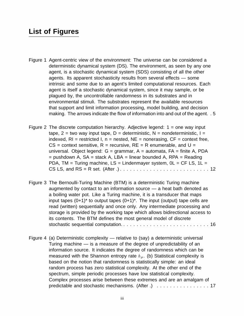
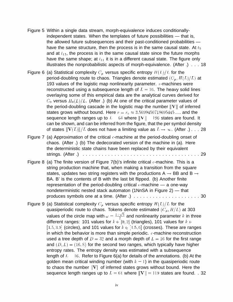


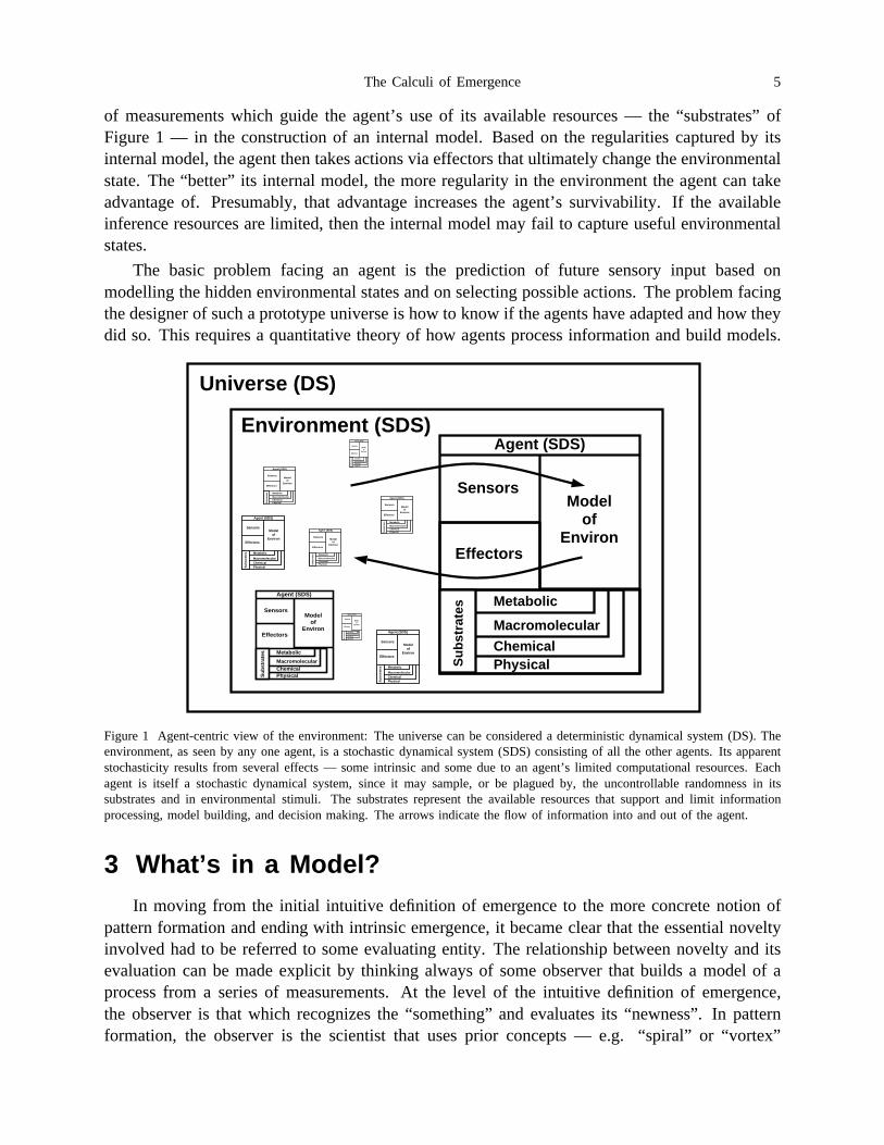
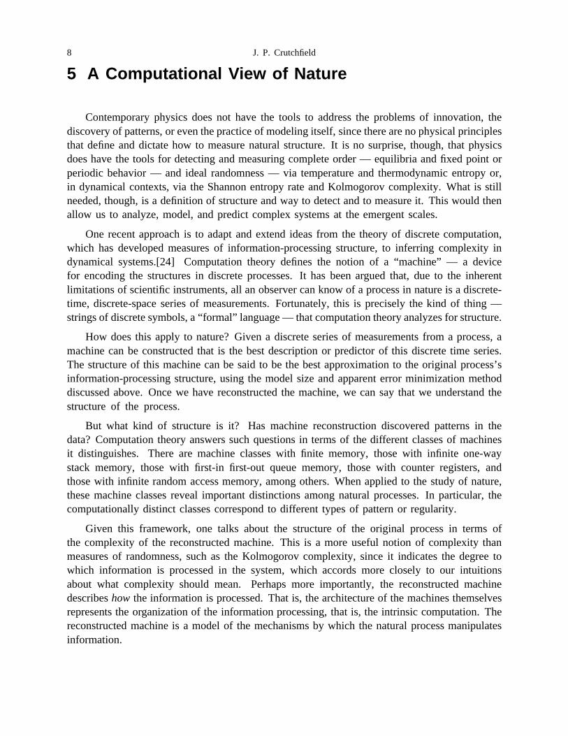
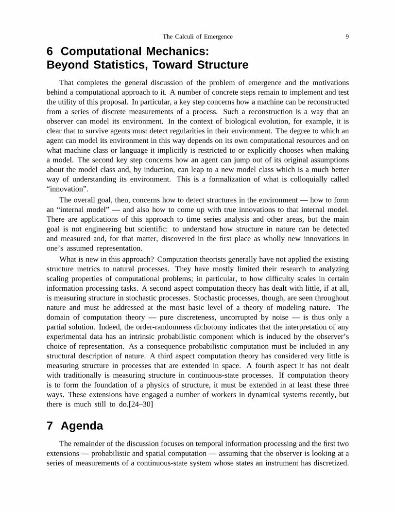
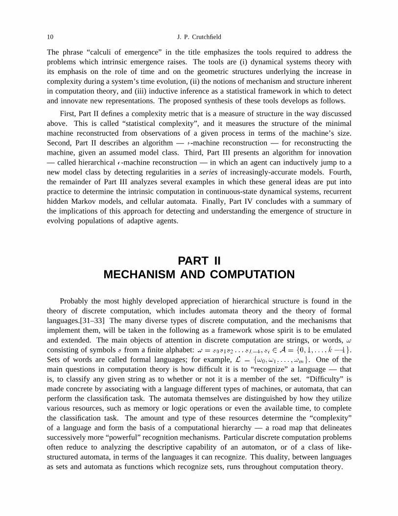
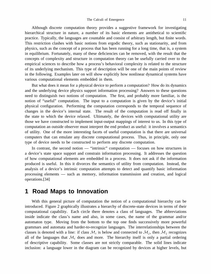
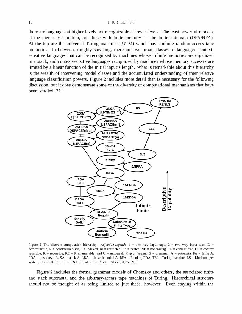
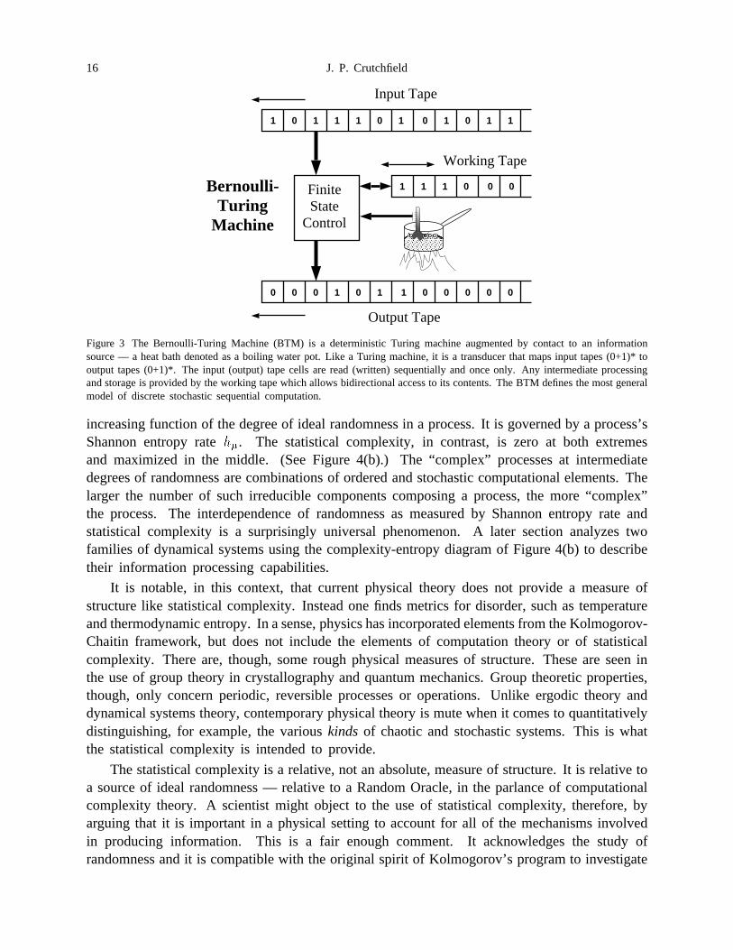
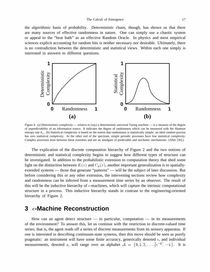
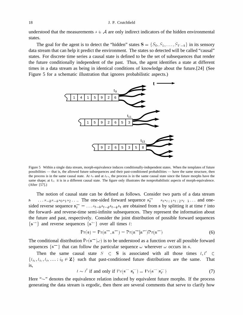
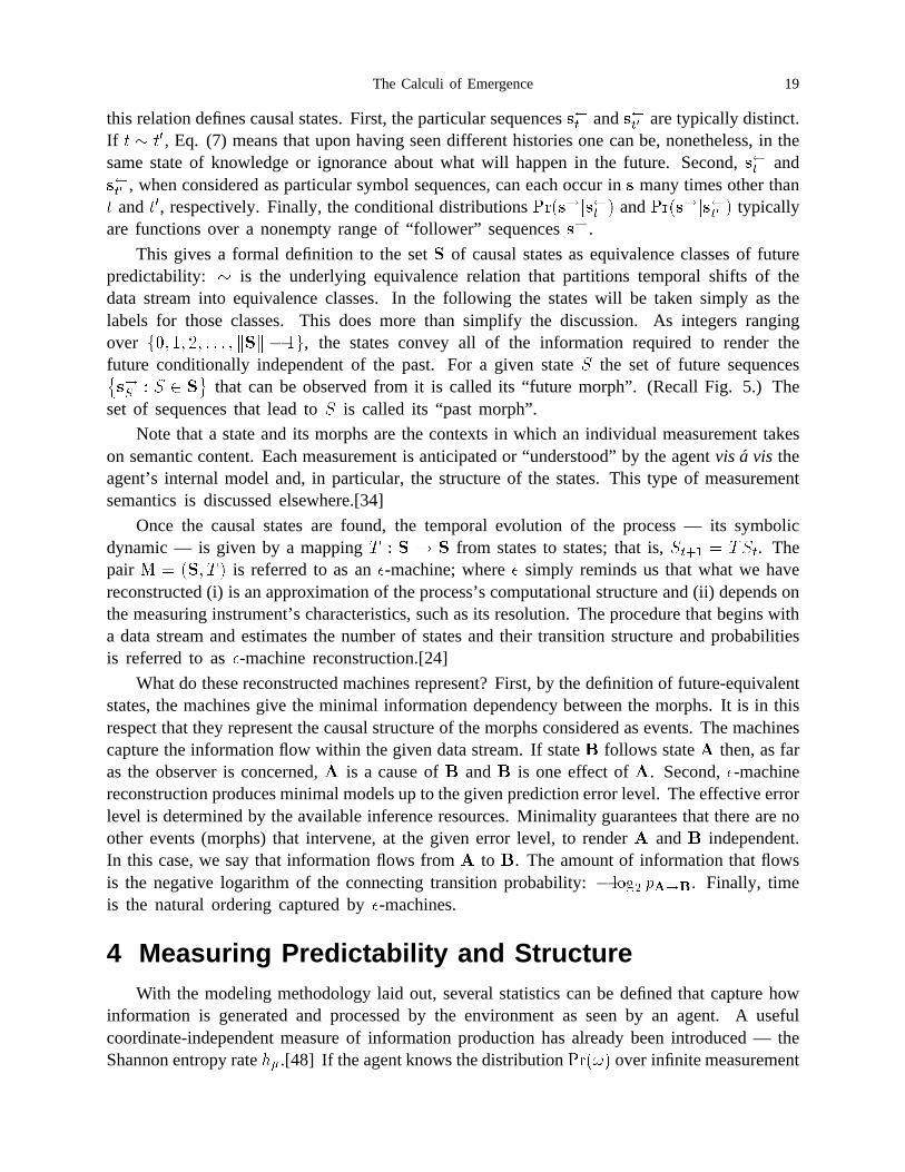
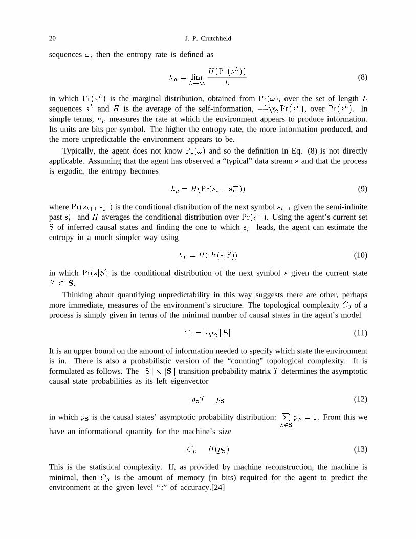
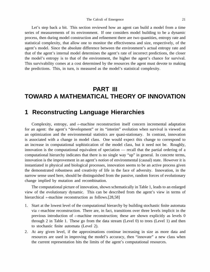
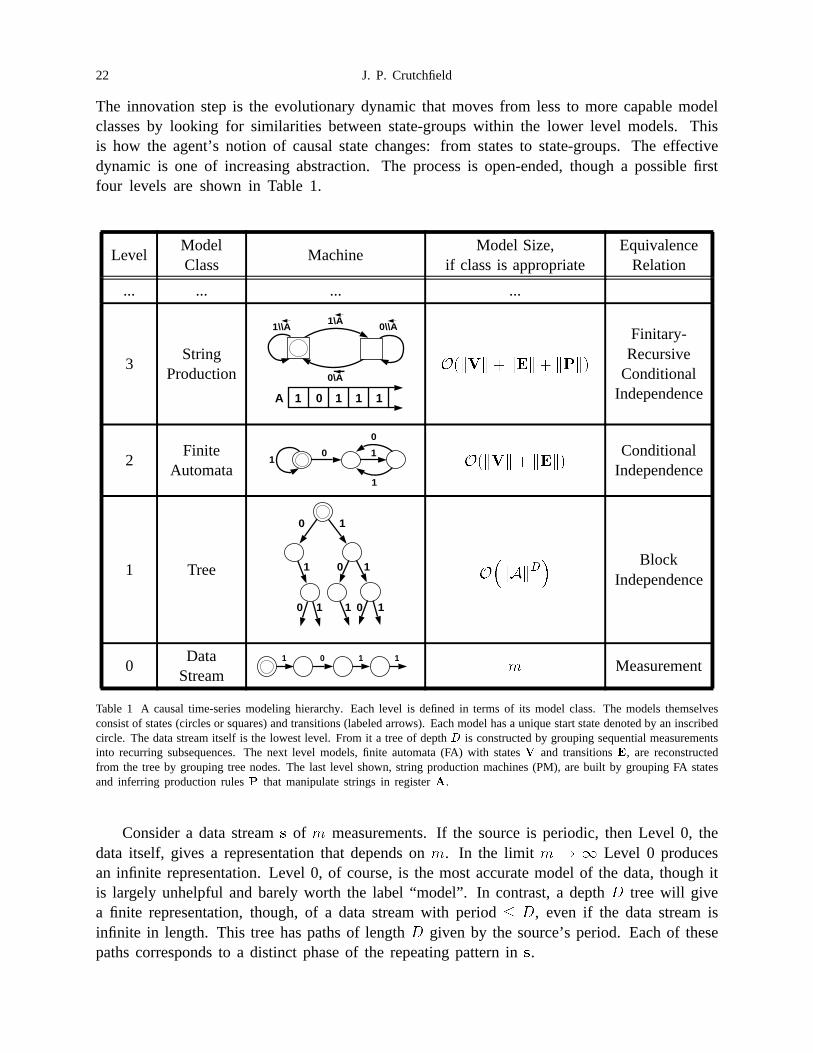
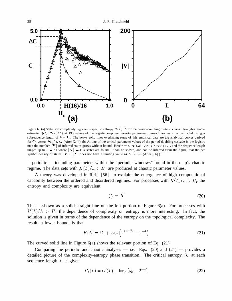
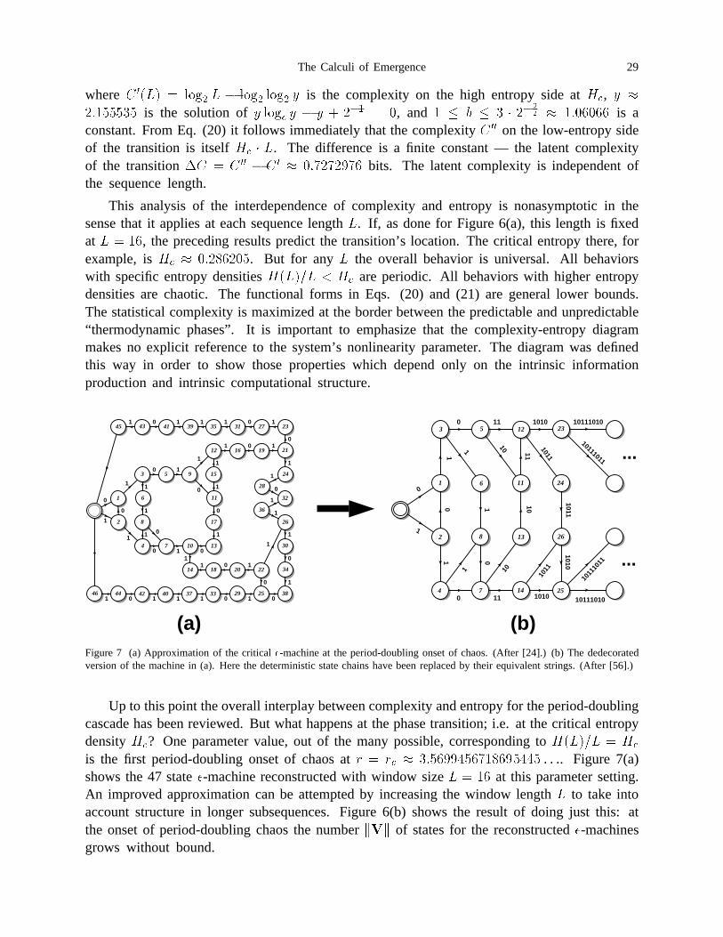
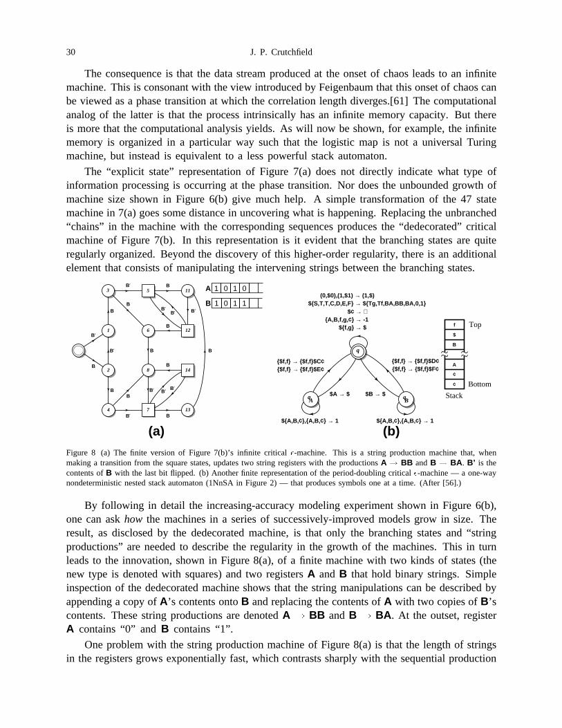
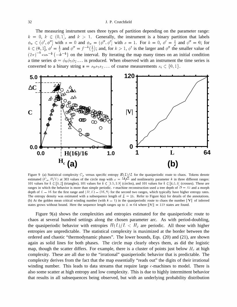
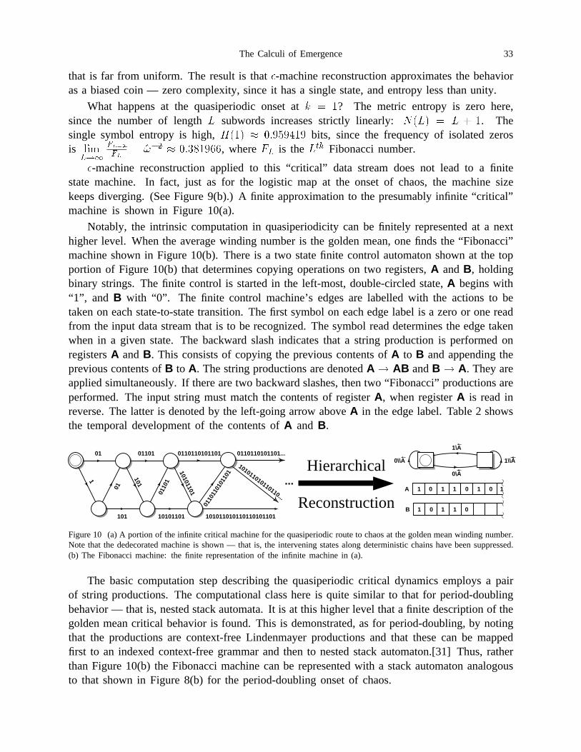
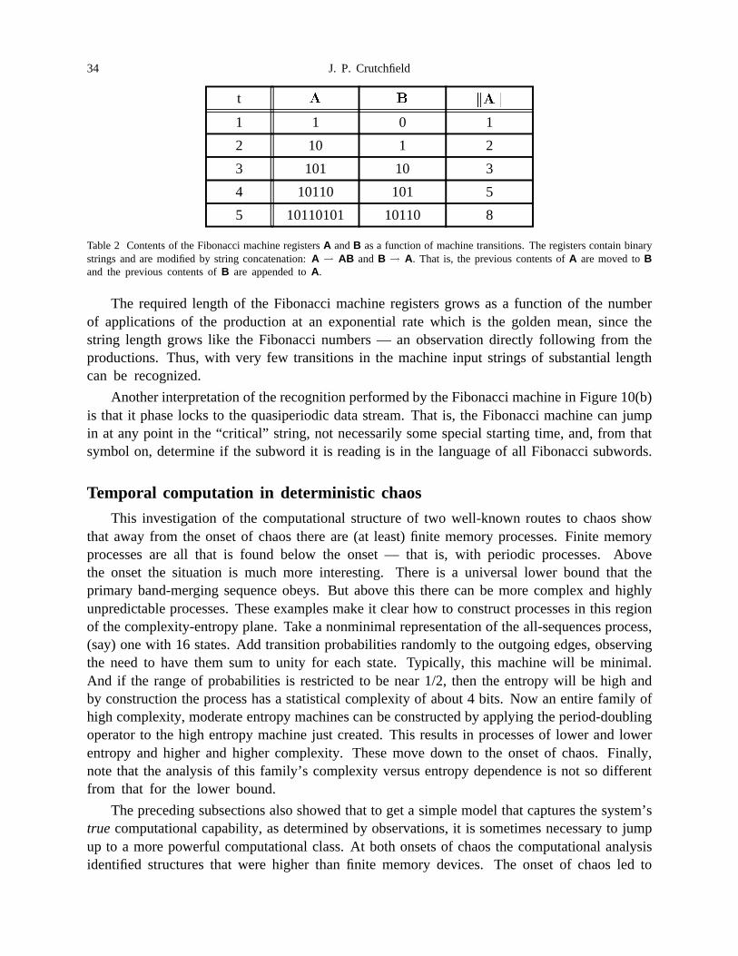
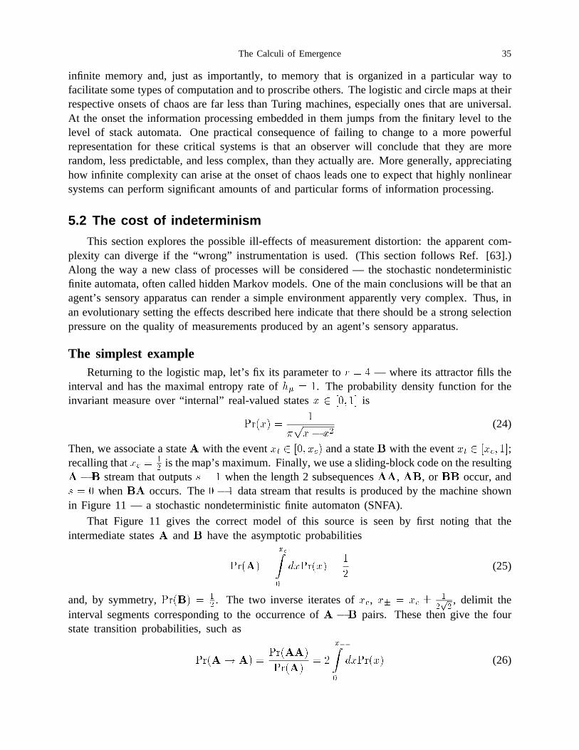
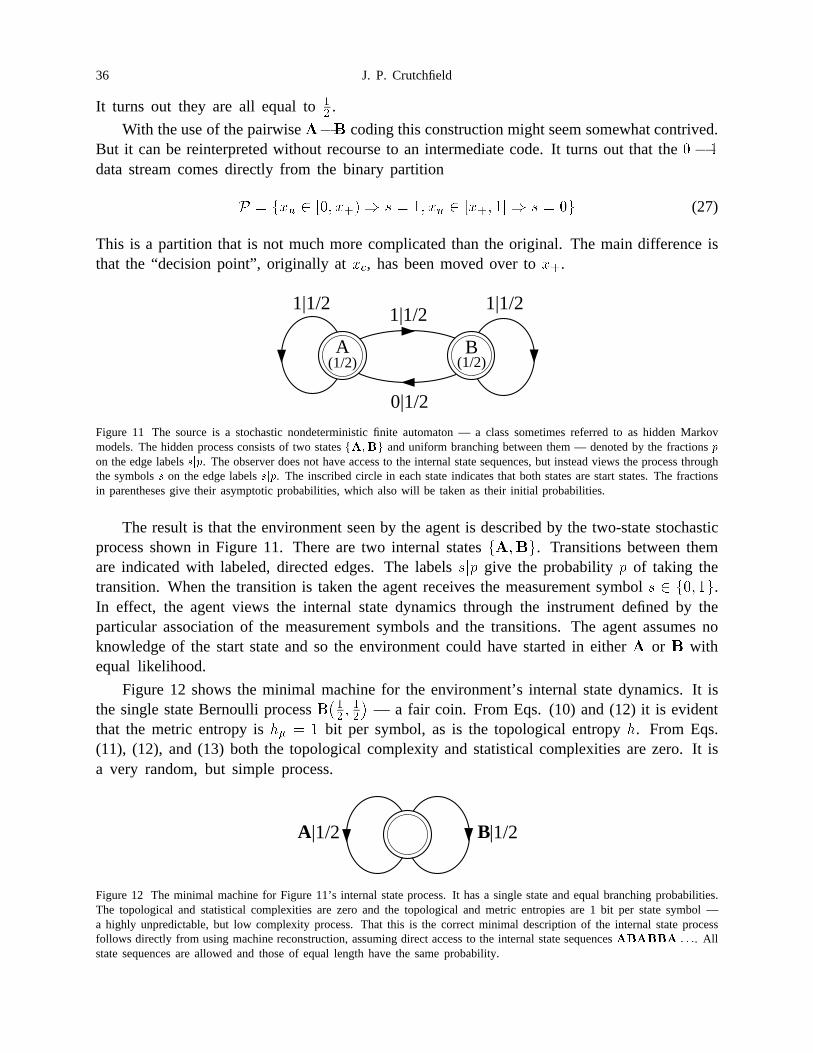
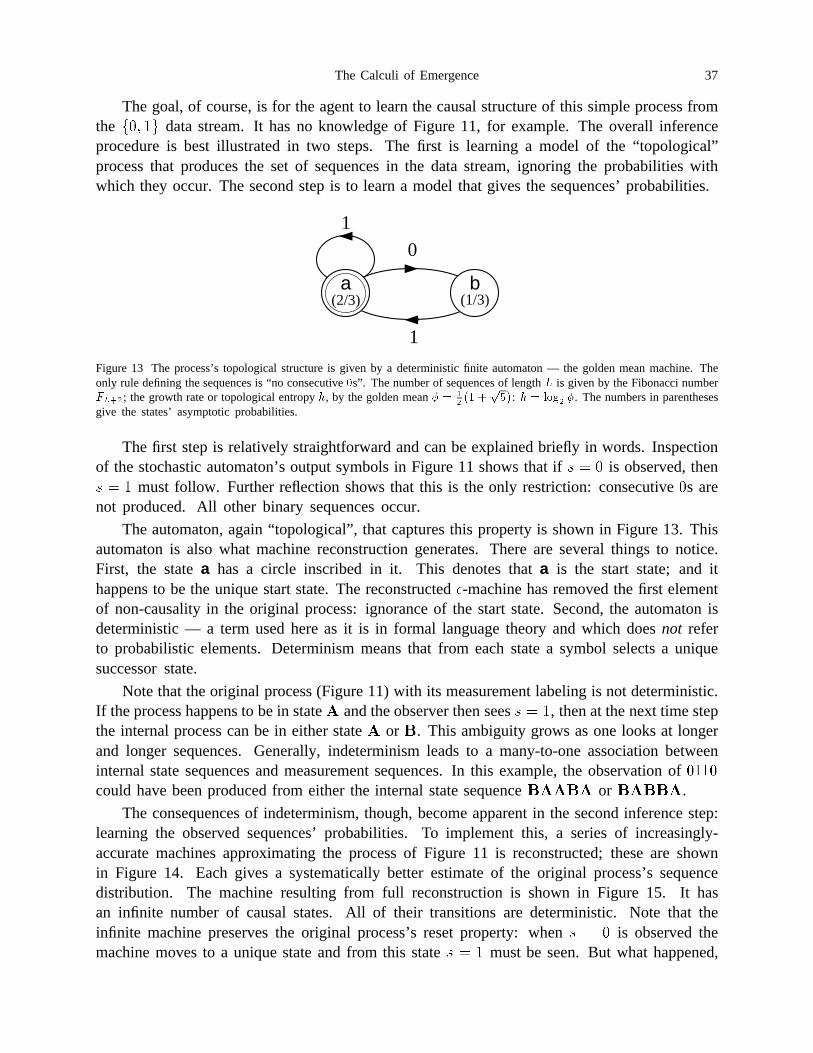
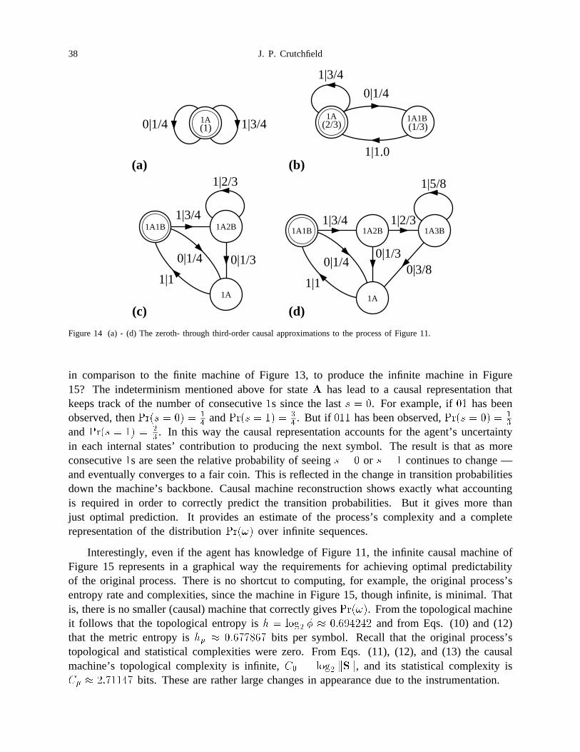
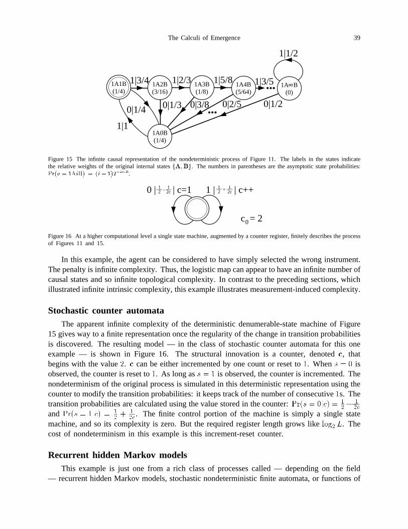

![Biological sequence annotation with hidden Markov modelscompbio.fmph.uniba.sk/papers/10nanasith.pdfHidden Markov Models A hidden Markov model (HMM) [DEKM98] is a frequently used generative](https://static.documents.pub/doc/80x56/5fb45168e0de87028d36a1d7/biological-sequence-annotation-with-hidden-markov-hidden-markov-models-a-hidden.jpg)


