The Calibration of Stochastic-Local Volatility Models -An Inverse Problem Perspective

Yuri F. Saporito∗, Xu Yang† and Jorge P. Zubelli‡

November 9, 2017

Abstract

We tackle the calibration of the so-called Stochastic-Local Volatility (SLV) model.This is the class of financial models that combines the local and stochastic volatilityfeatures and has been subject of the attention by many researchers recently. More pre-cisely, given a local volatility surface and a choice of stochastic volatility parameters,we calibrate the corresponding leverage function. Our approach makes use of regu-larization techniques from the inverse-problem theory, respecting the integrity of thedata and thus avoiding data interpolation. The result is a stable and robust algorithmwhich is resilient to instabilities in the regions of low probability density of the spotprice and of the instantaneous variance. We substantiate our claims with numericalexperiments using simulated as well as real data.

1 Introduction

The search for parsimonious models that would capture the market-observed smilebehavior in the implied volatility surface (IVS) is still one of the main research top-ics in Mathematical Finance. Among the different models that have been introduced,perhaps the two most important attempts are the Stochastic Volatility (SV) models,[Hes93] and [Gat06], and the Local Volatility (LV) model of [Dup94]. While SV modelscapture crucial stylized facts of the volatility dynamics, they cannot perfectly calibratethe IVS, especially for short maturities. On the other hand, the LV model was con-structed to fit any arbitrage-free IVS. However, it has poor dynamical properties, see[AN04]. A very important issue when considering these models is their calibrationto the market-observed IVS; we forward the reader to [AAYZ17, Kil11, MN04] andreferences therein for different calibration methods of SV and LV models, individually.

The Stochastic-Local Volatility (SLV) model is able to combine the best aspects ofeach one of such model classes, see [GHL11, LTZ14, TZL+15]. In the present articlewe shall present a stable and effective method to calibrate the SLV model that consistsof adapting the method proposed in [EE05] and [EHN96] to the SLV framework.

∗Escola de Matematica Aplicada (EMAp), Fundacao Getulio Vargas (FGV), Rio de Janeiro, Brazil,yuri.saporito@fgv.br†Instituto de Matematica Pura e Aplicada (IMPA), Rio de Janeiro, Brazil, xuyang@impa.br‡Instituto de Matematica Pura e Aplicada (IMPA), Rio de Janeiro, Brazil, zubelli@impa.br

1

arX

iv:1

711.

0302

3v1

[q-

fin.

CP]

8 N

ov 2

017

Although, separately, the calibration of SV and LV models has been extensivelydiscussed in the literature, to the best of our knowledge, there are three approaches tocalibrate an SLV model: [HL09, GHL11] and [TZL+15]. The first two are Monte Carlobased methods, while the last one relies on the numerical solution of a partial differentialequation (PDE). Since the method we propose here is also based on PDEs, we will useas benchmark the method presented [TZL+15]. Additionally, [WitH17] uses the samecalibration idea as in this benchmark method, but considers an adjoint method to solvethe related Fokker-Planck equation for the transition probability density, see Section3.1.1.

In order to exemplify our method, we consider two numerical exercises. One usessynthetic data generated from a known SLV model and the other uses real option datafrom an FX market. These examples corroborate to the theoretical conclusions of thecomparison of the benchmark and our proposed method. In fact, we verify that ourmethod is more robust against noise and more resilient to instabilities.

The paper is organized as follows. In Section 2, we briefly describe the SLV model.The benchmark and proposed calibration procedures are outlined in Section 3. Finally,in Section 4, we test our method with synthetic and real FX data.

2 Model Description

The Stochastic-Local Volatility (SLV) model assumes that, under a risk-neutral mea-sure, the spot price satisfies

dSt = (r − d)Stdt+√VtL(t, St)StdW

St ,

dVt = κ(m− Vt)dt+ ξ√VtdW

Vt ,

dWSt dW

Vt = ρdt.

(2.1)

The rates r and d are the risk-free interest rate and the dividend rate, respectively.In this version of the SLV model, we assume that the stochastic part of the volatil-ity is following the Heston model, [Hes93]. The parameters κ, m, ξ and ρ have thesame interpretation as in the pure SV model. Moreover, notice that this SLV modelsimplifies to the Heston model when L ≡ 1. With respect to our proposed calibrationprocedure, the choice of the SV model could have been easily modified. For exam-ple, we could have considered the SABR model of [HKLW02] or the Inverse Gammamodel of [LLZ16]. Additionally, it is fairly easy to extend the method presented here todeal with time dependent interest and dividend rates, as we consider in our numericalexamples. However, for cleaner exposition we will consider constant rates.

The function L is called the leverage function and it plays a very important role inthe model above. It is the ingredient that allows the model to perfectly calibrate theIVS seen in the market. In order to achieve this goal, the function L must satisfy (see[Gyo86])

σ2loc(t, S) = E[VtL

2(t, St) | St = S] = L2(t, S)E[Vt | St = S],(2.2)

where σloc is the local volatility function calibrated to the market, see Section 3.1.3.We define then

Σ(t, S) = E[Vt | St = S].(2.3)

2

It is important to notice that Equation (2.2) is an implicit equation for L, since it isneeded for the computation of Σ(t, S).

Note that the parameters of the SV part of the model may be (almost) freely chosen.Given a reasonable choice of parameters, choosing L to satisfy Equation (2.2) allowsthe model to fit any arbitrage-free IVS. The adjectives almost and reasonable used hererefer to the fact that the SDE (2.1) using formula (2.2) for L might not have a solutionfor certain choices of parameters, see Remark 3.1.

3 Calibration

In this section we shall discuss two different PDE techniques that can be applied tocalibrate an SLV model, namely the benchmark and our proposed method. For both,we will assume that the local volatility surface and the SV parameters of the modelhave been already computed.

Notice now that we can rewrite Equation (2.3) as

Σ(t, S) = E[Vt | St = S] =

∫ +∞0 V p(t, S, V )dV∫ +∞0 p(t, S, V )dV

,(3.1)

where p(t, ·, ·) is the joint density probability (St, Vt) and solves the Fokker-PlanckPDE:

∂p

∂t+

∂

∂S((r − d)Sp) +

∂

∂V(κ(m− V )p)− 1

2

∂2

∂S2(V L2(t, S)S2p)(3.2)

− 1

2

∂2

∂V 2(ξ2V p)− ∂2

∂S∂V(ρξV L(t, S)Sp) = 0,

with initial condition p(0, S, V ) = δ(S − S0)δ(V − V0), i.e. the Dirac mass at (S0, V0).

Remark 3.1 (Existence of Solution for SDE (2.1)). Using Equation (3.1), we mayrewrite the SDE (2.1) as

dSt = (r − d)Stdt+√VtσL(t, St)

√ ∫ +∞0 p(t, St, V )dV∫ +∞

0 V p(t, St, V )dVStdW

St ,

dVt = κ(m− Vt)dt+ ξ√VtdW

Vt ,

dWSt dW

Vt = ρdt.

(3.3)

This is called a McKean SDE, since the diffusion coefficient depends on the law of(S, V ). The existence of solutions of this SDE is a very challenging problem, andoutside the scope of this paper. For a discussion of this topic, see [GHL11] and [JZ17].For our work here, we will assume that the SDE has a unique strong solution.

Remark 3.2 (Mixing Fraction). Additional parameters could be considered in orderto calibrate some exotic derivatives (e.g. Barrier or Asian options). In particular, givensome fixed vol-of-vol, ξ, and correlation, ρ, one could define

ξλ = λξ and ρλ = λρ,

for λ ∈ [0, 1]. This parameter is usually called mixing fraction, as it mixes the stochas-tic and local aspects of the volatility. Notice that λ = 0 implies a pure LV model.

3

Moreover, the parameters ξ and ρ could be taken as the calibrated parameters of apure SV model. The goal is then to choose λ in order to calibrate a given exotic deriva-tive price. For instance, if we choose a down-and-out barrier Call option with barrierB and strike K > B, we could numerically solve the following PDE

∂P

∂t+ (r − d)S

∂P

∂S+

1

2vL2(t, S)S2∂

2P

∂S2+ κ(m− v)

∂P

∂v+

1

2λ2ξ2v

∂2P

∂v2(3.4)

+ λ2ξρvL(t, S)S∂2P

∂S∂V− rP = 0,

for S ∈ [B,+∞), with P (t, B, V ) = 0 and final condition P (T, S, V ) = (S −K)+. It isstraightforward to consider λ time-dependent.

Remark 3.3 (Monte Carlo Methods). For multi-factor SV models, both methodsdescribed in this paper require a high dimensional PDE solver to numerically deal withthe Fokker-Planck equation and therefore suffers from the curse of dimensionality. Thisissue would be circumvented using a Monte Carlo method. For instance, in [HL09],using the Markovian projection technique, an algorithm is proposed to calibrate theleverage function L. Additionally, in [GHL11], the authors applied the McKean’sparticle method, and developed an algorithm to hybrid models, where the short-termrate and the volatility are modeled as diffusions.

3.1 Numerical Aspects

There are some common numerical aspects for both benchmark and our calibrationprocedures, and we will state them here. Firstly, since the methods considered hereare based on finite difference methods for PDEs, we will consider discrete meshes fortime, spot price and spot volatility. A (uniform) mesh for a variable y depends on achoice for a finite lower bound ymin, a finite upper bound ymax and a step size ∆y. Itis assumed that Ny = (ymax − ymin)/∆y ∈ N. The mesh for y is then

yi = ymin + i∆y, for i = 0, . . . , Ny.

In our case, we will assume that tmin = Smin = Vmin = 0. We will use the sub-indexn for t, i for S and j for V . One could surely use non-uniform meshes, but we willpresent the results here with uniform meshes for clearer illustration.

3.1.1 Numerical Methods for the Fokker-Planck PDE

The Fokker-Planck PDE, shown in Equation (3.2), will have to be numerically solvedgiven the parameters of the SV model and a fixed leverage function L. That is, discretiz-ing the Fokker-Planck PDE with any chosen method, we will compute an approxima-tion for p(tn, Si, Vj). A sensible choice for the discretization method is of AlternatingDirection Implicit (ADI) type, see [itHF10]. Namely, in our numerical example, weconsider the Douglas scheme, which was proposed in [DR56]. Moreover, the choice ofboundary conditions for the numerical method is also very important. We have chosenthe zero flux condition, see for instance [Luc12].

Note that, by using an ADI method to solve for the Fokker-Planck equation,p(tn, ·, ·) would depend on L(tn, ·) and L(tn−1, ·). However, the benchmark methodassumes that p(tn, ·, ·) only depends on L(tn−1, ·). For more details, see Appendix A.

In a different direction, one could consider adjoint methods to numerically solvethe Fokker-Planck PDE as in [WitH17].

4

3.1.2 Approximation of the Initial Condition

The initial condition for our Fokker-Planck PDE is not well-behaved; it is a Diracmass at the point (S0, V0). In order to avoid numerical issues arising from this lack ofsmoothness, we consider a smooth approximation of this Dirac mass. Specifically, weuse a bivariate normal distribution with small variances to represent the initial density:

p(0, S, V ) =1

2πσSσVexp

{− 1

2σ2S

(S − S0)2 − 1

2σ2V

(V − V0)2

}.(3.5)

In our numerical experiment, we have used σ2S = σ2

V = 10−3. See, for instance,[TZL+15] for details.

3.1.3 Numerical Computation of the Local Volatility

The calibration of local volatility surfaces is an important inverse problem in Math-ematical Finance. In [Dup94], the author has proposed the local volatility model, inwhich the European options prices satisfy the PDE of the form

∂C

∂T+ (r − d)K

∂C

∂K− 1

2σ2loc(T,K)K2 ∂

2C

∂K2+ dC = 0, T > 0,K > 0,(3.6)

with initial and boundary conditions given by

C(0,K) = (S0 −K)+,(3.7)

limK→∞

C(T,K) = 0,

limK→0

C(T,K) = S0,

where C = C(T,K) is the value of the European call option with expiration date Tand strike price K. The inverse problem of the local volatility model is that, giventhe options prices {C(T,K)}T,K , we want to find a plausible local volatility surface,{σloc(T,K)}T,K , which can explain these options prices. Two of the challenges ofthis inverse problem are the ill-posedness, [CCZ12], and the scarceness of the data ofoptions prices, [AAYZ17]. To solve an ill-posed inverse problem, one popular methodis to use the Tikhonov regularization [ACZ16, AZ14, CCZ12, CZ15, ACZ17]. We willbriefly introduce this regularization method in Section 3.3. To solve the problem of thescarceness of the data, one possibility is to interpolate/extrapolate the data of optionsprices to all the locations of the mesh, [Kah05]. In this paper, however, we apply themethod discussed in [AAYZ17, AAZ17], where we use a P matrix to map the gridlocations of the estimated options prices to those of real data.

3.2 Benchmark Method

In this section, we will describe the method proposed in [RMQ07] and further developedin [TZL+15], which is our benchmark method. From Equation (2.2), we have

L(t, S) =σloc(t, S)√

Σ(t, S)= σloc(t, S)

√√√√ ∫ +∞0 p(t, S, V )dV∫ +∞

0 V p(t, S, V )dV.

5

The benchmark calibration procedure is based on the equation above. As we havepreviously mentioned, this is an implicit equation for L, since p depends on it. Moreprecisely, the leverage function is initialized at Si as

LB0,i := σloc(0, Si)

√√√√ ∑NVj=0 p0,i,j∆V∑NVj=0 Vjp0,i,j∆V

,(3.8)

with p0,i,j given by Equation (3.5). We are using the superscript B to denote thatthis is the leverage function computed by the benchmark method. Assuming we havecomputed LB at time tn, we use the numerical method discussed in Section 3.1.1to solve the Fokker-Planck Equation (3.2) from tn to tn+1 with L(t, Si) = LBn,i, fort ∈ [tn, tn+1]. Hence, we find an approximation for p(tn+1, Si, Vj), which we will denoteby pBn+1,i,j . Finally, we set

LBn+1,i := σloc(tn+1, Si)

√√√√ ∑NVj=0 p

Bn+1,i,j∆V∑NV

j=0 VjpBn+1,i,j∆V

,(3.9)

and repeat the procedure above.

Algorithm 1 Benchmark Algorithm of [RMQ07]

1: Set the initial condition of p0,i,j and LB0,i using Equations (3.5) and (3.8), respectively.2: for n = 0, 1, 2, . . . , Nt − 1 do3: Set L(t, Si) = LBn,i, for t ∈ [tn, tn+1].

4: Solve the Fokker-Planck PDE (3.2) in t ∈ [tn, tn+1].

5: Update LBn+1,i with Equation (3.9).6: end for7: return LBn,i for n = 0, . . . , Nt and i = 0, . . . , NS.

3.3 Proposed Method

The problem under consideration is a classical example of an ill-posed inverse problem.We shall now provide some background on inverse problems in general and on ourspecific problem.

Ill-posed problems have been treated extensively in the literature since they arerelevant in several fields, see [Vog02] and references therein. Amongst the main tech-niques to address these problems, it is safe to say that one of the most well-known isthe so-called Tikhonov regularization. It consists basically in transforming the problemunder consideration, say that of trying to solve F (x) = y, into a minimization of theform

arg min ||F (x)− y||2 + α|||x− x0|||2,

where || · || and ||| · ||| are two norms, and x0 incorporates the a priori informationthat will allow the regularization of the problem. By changing the scale factor α of thenorm ||| · |||, one would put more or less emphasis on such a priori information. Theoptimal choice of α is the subject of intense investigation. Among the more well-knownmethods one can cite the discrepancy principle and the L-curve method, see [Vog02].

6

Further, developments led to the use of other metrics (or more generally functionalsinstead of norms), see [KNS08] and references therein.

Let Ln,i be the leverage function at time tn and spot price Si, where n = 0, 1, . . . , Nt

and i = 0, 1, . . . , NS , computed using our proposed method described below. Then thedensity function p(tn+1, ·, ·) is computed by the numerical method discussed in Section3.1.1 to solve the Fokker-Planck Equation (3.2) from tn to tn+1 with L(t, Si) = Ln,i,for t ∈ [tn, tn+1]. We denote this approximation by pn+1,i,j . Define G1 the operator

that associates a given {Ln,i}NSi=0 to the corresponding approximation of this density:

(3.10) {pn+1,i,j}NS ,NVi,j=0 =: G1({Ln,i}NS

i=0).

The initialization {L0,i}NSi=0 will be discussed in the sequel.

Fix now {yi}NSi=0 and let G2 be the operator mapping a choice of leverage function

equals {yi}NSi=0 to the local volatility function at time tn following Equation (2.2),

G2({yi}NSi=0, {pn,i,j}

NS ,NVi,j=0 ) :=

yi√√√√∑NV

j=0 Vjpn,i,j∆V∑NVj=0 pn,i,j∆V

NS

i=0

.(3.11)

Notice

G2({yi}NSi=0, {pn,i,j}

NS ,NVi,j=0 ) = G2({yi}NS

i=0,G1({Ln−1,i}NSi=0)) =: G({yi}NS

i=0, {Ln−1,i}NSi=0)

i.e. G is the operator that takes {Ln−1,i}NSi=0 and {yi}NS

i=0 to the local volatility at timetn. Therefore, in order to obtain the surface of the leverage function, we have to solvethe following Tikhonov-type optimization problem for n = 1, 2, . . . , Nt.

{Ln,i}NSi=0 := arg min

{yi}NSi=0

‖σloc(tn, ·)− G({yi}NSi=0, {Ln−1,i}NS

i=0)‖2Γ−1(3.12)

+ α1‖{yi}NSi=0 − {Ln−1,i}NS

i=0‖2D−1

0+ α2‖RS{yi}NS

i=0‖2D−1

S,

where Γ, D0 and DS are chosen symmetric positive definite covariance matrices.We define the vector norm ‖x‖C =

√xTCx and RS is the matrix representing

the finite-difference approximation of the linear operator ∂S. The initial value{L0,i}NS

i=0 is chosen by solving the minimization (3.12) with L−1,i = c, for alli = 0, . . . , NS, for some chosen constant.

Algorithm 2 Proposed Algorithm

1: Set the initial condition of {p0,i,j}NS ,NVi,j=0 using Equation (3.5) and set {L−1,i}NS

i=0 to achosen constant.

2: for n = 0, 1, 2, . . . , Nt do3: Solve the minimization problem (3.12) for {Ln,i}NS

i=0.

4: If n < Nt solve the finite difference problem in (3.10) for {pn+1,i,j}NS ,NVi,j=0 .

5: end for6: return Ln,i for n = 0, . . . , Nt and i = 0, . . . , NS.

7

4 Numerical Example

We will now compare the methods described in Sections 3.2 and 3.3 within syn-thetic and real data examples. The following information is common to bothcases:

Variable Lower Bound Upper Bound Fine Mesh Coarse Mesh

time 0 1 0.001 0.025log-moneyness -3 3 0.025 0.05volatility 0 1 0.005 0.01

Table 1: Mesh parameters

The coarse mesh is the one used in the finite difference methods in our nu-merical examples below.

Figure 1: Domestic and foreign interest rates

4.1 Synthetic Data

In this synthetic data example, we suppose the ground truth leverage function(see Figure 2) is given by

(4.1) L(t, x) := 1.14 cos(2πxt), where x ∈ [−3, 3], t ∈ [0, 1].

We calculate Σ(t, x) and local volatility surface σloc based on this given L in thefine mesh. The details of the mesh for maturity, log-moneyness and volatility aregiven in the Table 1. We then add a relative noise to the local volatility surface

(4.2) σloc(t, x)η := σloc(t, x)(1 + 0.01ηt,x)

where ηt,x are independent draws from the standard normal distribution N (0, 1).In order to avoid the so-called inverse crime ([KS06]), we sample the data to acoarser mesh, which is also given in Table 1. Figure 2 presents the noisy localvolatility surface. The parameters of the SV part of the model are given in Table2. The Tikhonov parameters are α1 = 0 and α2 = 10−2, see Equation (3.12).

8

Parameter Value

V0 0.04κ 2m 0.04ξ 0.25ρ -0.5

Table 2: SV parameters for the synthetic data example

Figure 2: The ground truth leverage function (left) and the local volatility surface σloc(t, x)η

(right).

4.2 Real Data

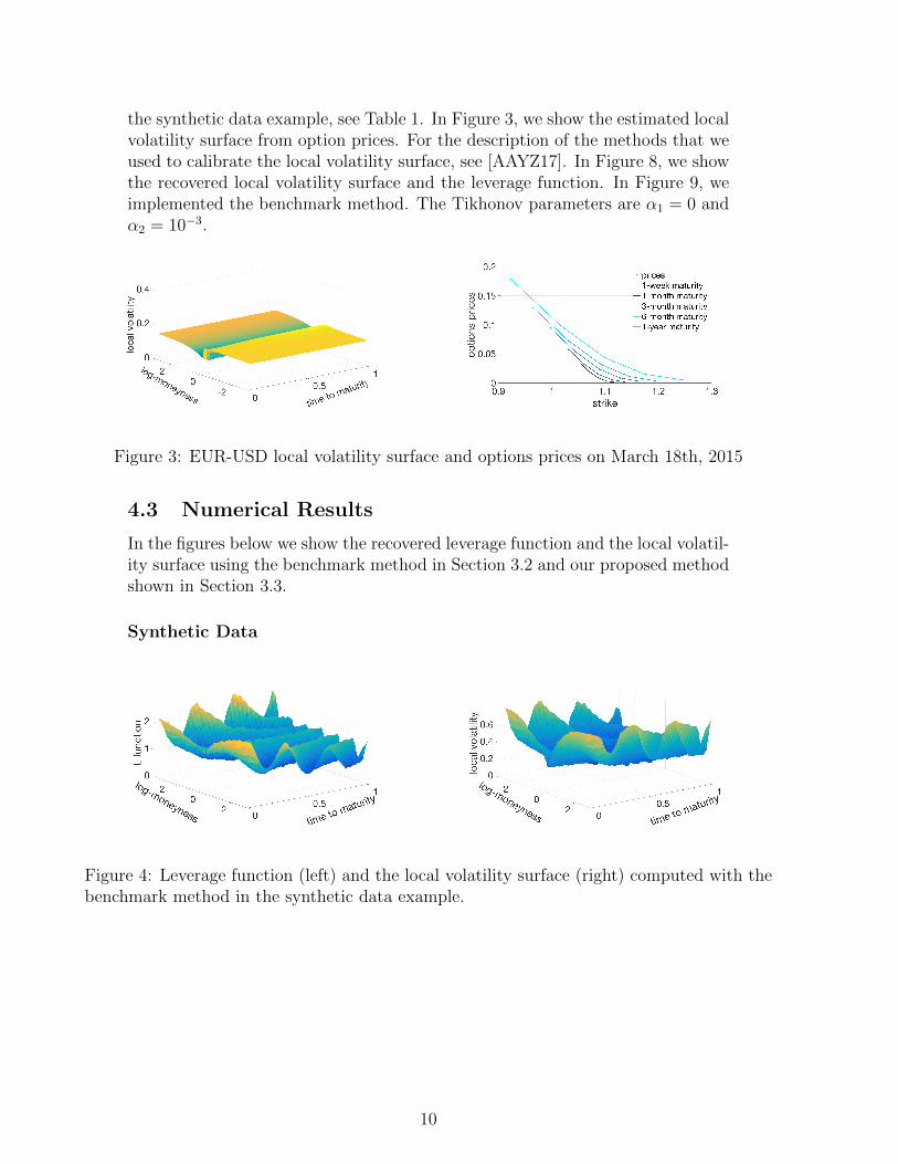
In this section we present a real data example. We chose FX options on EURUSDon March 18th, 2015. They include the typical 25 liquid option contracts, with5 maturities (1W, 1M, 3M, 6M, 1Y) and 5 strikes (related to 10 and 25 Call andPut Delta and to ATM) per maturity (see Figure 3). The spot value was 1.0864.The parameters of the Heston model are calibrated to this data set and given inTable 3.

Parameter Value

V0 0.013κ 1.025m 0.013ξ 0.161ρ -0.626

Table 3: SV parameters calibrated to real data

These parameters were required to satisfy the Feller condition. This translatesinto more realistic dynamics for the volatility, since it prevents the volatilityprocess V to reach the zero boundary. The domestic and foreign interest ratesare the same as in Figure 1. We choose the same discretization parameters as in

9

the synthetic data example, see Table 1. In Figure 3, we show the estimated localvolatility surface from option prices. For the description of the methods that weused to calibrate the local volatility surface, see [AAYZ17]. In Figure 8, we showthe recovered local volatility surface and the leverage function. In Figure 9, weimplemented the benchmark method. The Tikhonov parameters are α1 = 0 andα2 = 10−3.

Figure 3: EUR-USD local volatility surface and options prices on March 18th, 2015

4.3 Numerical Results

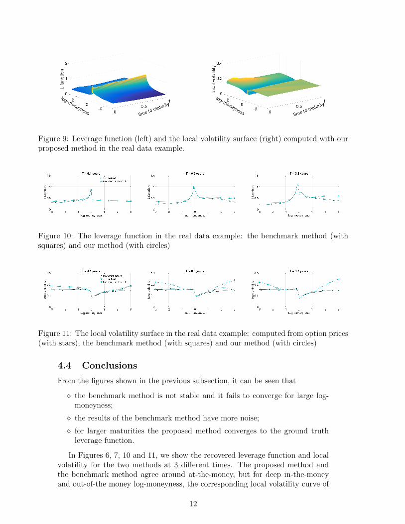
In the figures below we show the recovered leverage function and the local volatil-ity surface using the benchmark method in Section 3.2 and our proposed methodshown in Section 3.3.

Synthetic Data

Figure 4: Leverage function (left) and the local volatility surface (right) computed with thebenchmark method in the synthetic data example.

10

Figure 5: Leverage function (left) and the local volatility surface (right) computed with ourproposed method in the synthetic data example.

Figure 6: The leverage function in the synthetic data example: the ground truth (with stars),the benchmark method (with squares) and our method (with circles)

Figure 7: The local volatility surface in the synthetic data example: the ground truth (withstars), the benchmark method (with squares) and our method (with circles)

Real Data

Figure 8: Leverage function (left) and the local volatility surface (right) computed with thebenchmark method in the real data example.

11

Figure 9: Leverage function (left) and the local volatility surface (right) computed with ourproposed method in the real data example.

Figure 10: The leverage function in the real data example: the benchmark method (withsquares) and our method (with circles)

Figure 11: The local volatility surface in the real data example: computed from option prices(with stars), the benchmark method (with squares) and our method (with circles)

4.4 Conclusions

From the figures shown in the previous subsection, it can be seen that

� the benchmark method is not stable and it fails to converge for large log-moneyness;

� the results of the benchmark method have more noise;

� for larger maturities the proposed method converges to the ground truthleverage function.

In Figures 6, 7, 10 and 11, we show the recovered leverage function and localvolatility for the two methods at 3 different times. The proposed method andthe benchmark method agree around at-the-money, but for deep in-the-moneyand out-of-the money log-moneyness, the corresponding local volatility curve of

12

the benchmark method is distant from the market’s local volatility surface. Wehave shown three maturities, but this phenomenon can also be observed for theother maturities. This phenomenon is observed less prominently in the syntheticdata example and the reason is that the local volatility surface is smoother.

Once we estimate the leverage function L, we can recover the local volatilitysurface using the Alternating Direction Implicit (ADI) method for the Fokker-Planck PDE with the leverage function at both times, tn and tn+1, see Section3.1.1. Comparing with the ground truth of local volatility surface in the syntheticdata example, we can calculate the relative residuals. In Table 4, we present therelative residuals in two intervals of the log-moneyness, which are [−3, 3] and[−2, 2]. We also report the relative residuals of the real data example. For bothexamples, we see that the proposed method generates better results with relativeerrors significantly smaller than the benchmark method. We would like to pointout that this failure of convergence of the benchmark method is not relatedto a boundary issue. Indeed, numerical experiments on smaller log-moneynessintervals have similar results to the truncated version of the results we have found.

Example Benchmark in [−3, 3] (in [−2, 2]) Proposed in [−3, 3] (in [−2, 2])

Synthetic 7.92% (2.07%) 1.40% (1.09%)Real 27.82% (15.44%) 7.93% (5.44%)

Table 4: Relative residuals

The conclusion from our numerical exercises, that corroborates the theoreticalreasoning, is that, when compared to the benchmark, the proposed method

� is more robust against noise;

� is more resilient to instabilities in the regions of low probability density ofthe spot prices and instantaneous variance;

� does not require ad hoc procedures to avoid instabilities due to low proba-bility regions.

� respects the data in the sense that we do not apply interpolation. Moreprecisely, the benchmark method requires the knowledge of the local vol onthe same mesh as the one used for the Fokker-Planck Equation (3.2).

5 Concluding Remarks

We have studied the calibration of the Stochastic-Local Volatility model andproposed a numerical method based on the Tikhonov regularization framework.We compared this proposed method with a benchmark method based on PDEtechniques defined in [TZL+15] with two different numerical examples. Underboth cases, we have observed that the proposed method is more robust and hassignificantly smaller relative error when compared to the benchmark method.

Since our proposed method is aimed to improve the error created by usingEquation (3.9) to updated the leverage function, we would have observed the

13

same improvement documented in Section 4.4 if we had used the adjoint methodproposed in [WitH17] to solve the related Fokker-Planck PDE.

Future development could consider the implementation of the online cali-bration procedure of [AAZ17]. This could not be achieved for the benchmarkmethod. Another avenue would be to explore the fast mean reversion stochasticvolatility setting conjoined with the local volatility surface estimation as de-scribed in [NP06].

A Specification of the ADI method

To solve Equation (3.2) numerically, we apply the finite difference Douglas-Rachford (DR) method [DR56]. For completeness, we shall now give the detailsof the implementation.

We suppose (t, S, V ) ∈ [tmin, tmax]× [Smin, Smax]× [Vmin, Vmax]. The discretiza-tion contains NS + 1 nodes in S direction, NV + 1 nodes in v direction andNt + 1 nodes in t direction. By using the central difference for the first-orderdifferentiation, all partial differentiations could be approximated as follows:

∂(Sp)

∂S≈ Si+1pn,i+1,j − Si−1pn,i−1,j

2∆S=:

δSSpn,i,j2∆S

∂((m− V )p

)∂V

≈ (m− Vj+1)pn,i,j+1 − (m− Vj−1)pn,i,j−1

2∆V=:

δm−VV pn,i,j2∆V

∂2(V L2(tn, S)S2p

)∂S2

≈ 1

(∆S)2(VjL

2(tn, Si+1)S2i+1pn,i+1,j

− 2VjL2(tn, Si)S

2i pn,i,j + VjL

2(tn, Si−1)S2i−1pn,i−1,j)

=:δV L2(t,S)S2

SS pn,i,j(∆S)2

∂2(V p)

∂V 2≈ Vj+1pn,i,j+1 − 2Vjpn,i,j + Vj−1pn,i,j−1

(∆V )2=:

δVV V pn,i,j(∆V )2

∂2(V L(tn, S)Sp

)∂S∂V

≈ 1

4∆S∆V(Vj+1L(tn, Si+1)Si+1pn,i+1,j+1+

Vj−1L(tn, Si−1)Si−1pn,i−1,j−1 − Vj+1L(tn, Si−1)Si−1pn,i−1,j+1−Vj−1L(tn, Si+1)Si+1pn,i+1,j−1)

=:δV L(t,S)SSV pn,i,j4∆S∆V

We replace the derivative in Equation (3.2) by these finite difference quotients.We then define the discretized system for the approximation pn,i,j for p(tn, Si, Vj)given by the θ-scheme:

(1− θA1 − θA2)p(n+1) = [1 + A0 + (1− θ)A1 + (1− θ)A2]p(n) +O(∆t3)

for n = 0, 1, 2, . . . , Nt − 1, where p(n) = {pn,i,j}NS ,NVi,j=0 , θ ∈ [0, 1] and

A0 :=1

4ρξRSV δ

V L(t,S)SSV ,

14

A1 := RS2δV L2(t,S)S2

SS +1

2(r − d)RSδ

SS ,

A2 := ξ2RV 2δVV V +

1

2κRV δ

m−VV ,

RS :=∆t

∆S, RV :=

∆t

∆V, RS2 :=

∆t

∆S2, RV 2 :=

∆t

∆V 2, RSV :=

∆t

∆S∆V.

The Douglas-Rachford method (DR method) is then defined as:

(1− θA1)W = [1 + A0 + (1− θ)A1 + A2]p(n)

(1− θA2)p(n+1) = W − θA2p(n)

Note that, here, for notational reason, we assume the rate r−d is constant. Inour experiment, with a slight modification of A1 and A2, we developed the methodfor the case of r−d being time-dependent and also the zero flux condition[Luc12].

References

[AAYZ17] V. Albani, U. Ascher, X. Yang, and J.P. Zubelli. Data driven recoveryof local volatility surfaces. Inverse Problems and Imaging, 11:2–2,2017.

[AAZ17] V. Albani, U. Ascher, and J.P. Zubelli. Local volatility models incommodity markets and online calibration. Journal of ComputationalFinance, 21:1–33, 2017.

[ACZ16] V. Albani, A. De Cezaro, and J.P. Zubelli. On the choice of theTikhonov regularization parameter and the discretization level: adiscrepancy-based strategy. Inverse Probl. Imaging, 10(1):1–25, 2016.

[ACZ17] V. Albani, A. De Cezaro, and J.P. Zubelli. Convex regularization oflocal volatility estimation. International Journal of Theoretical andApplied Finance, 20(01):1750006, 2017.

[AN04] C. Alexander and L. M. Nogueira. Stochastic local volatility. InProceedings of the Second IASTED, Nobember 2004.

[AZ14] V. Albani and J.P. Zubelli. Online local volatility calibration by con-vex regularization. Appl. Anal. Discrete Math., 8(2):243–268, 2014.

[CCZ12] A. De Cezaro, O. Cherzer, and J.P. Zubelli. Convex regularization oflocal volatility models from option prices: convergence analysis andrates. Nonlinear Anal., 75(4):2398–2415, 2012.

[CZ15] A. De Cezaro and J.P. Zubelli. The tangential cone condition for theiterative calibration of local volatility surfaces. IMA J. Appl. Math.,80(1):212–232, 2015.

[DR56] J. Douglas and H. Rachford. On the numerical solution of heat con-duction problems in two and three space variables. Transactions ofthe American mathematical Society, 82(2):421–439, 1956.

15

[Dup94] B. Dupire. Pricing with a smile. Risk, 7(1):18–20, 1994.

[EE05] H. Egger and H.W. Engl. Tikhonov regularization applied to theinverse problem of option pricing: convergence analysis and rates.Inverse Problems, 21(3):1027–1045, 2005.

[EHN96] H. W. Engl, M. Hanke, and A. Neubauer. Regularization of inverseproblems, volume 375. Springer Science & Business Media, 1996.

[Gat06] J. Gatheral. The Volatility Surface - A Practitioner’s Guide. Wiley,2006.

[GHL11] J. Guyon and P. Henry-Labordere. The Smile Calibration ProblemSolved. Risk, 2011.

[Gyo86] I. Gyongy. Mimicking the One-Dimensional Marginal Distributions ofProcesses Having an Ito Differential. Probab. Theory Related Fields,71(4):501–516, 1986.

[Hes93] S. L. Heston. A Closed-Form Solution for Options with StochasticVolatility with Applications to Bond and Currency Options. TheReview of Financial Studies, 6(2):327–343, 1993.

[HKLW02] P. S. Hagan, D. Kumar, A. S. Lesniewski, and D. E. Woodward.Managing Smile Risk. Wilmott Magazine, 2002.

[HL09] P. Henry-Labordere. Calibration of Local Stochastic Volatility Mod-els: A Monte-Carlo Approach. Risk, 2009. Extended version athttp://ssrn.com/abstract=1493306.

[itHF10] K.J. in ’t Hout and S. Foulon. ADI Finite Difference Schemes forOptions Pricing in the Heston Model with Correlation. Int. J. Numer.Anal. Model., 7(2):303–320, 2010.

[JZ17] B. Jourdain and A. Zhou. Existence of a calibrated regime switchinglocal volatility model and new fake brownian motions. arXiv preprintarXiv:1607.00077, 2017.

[Kah05] N. Kahale. Smile interpolation and calibration of the local volatilitymodel. Risk Magazine, 1(6):637–654, 2005.

[Kil11] F. Kilin. Accelerating the Calibration of Stochastic Volatility Models.The Journal of Derivatives, 18(3):7–16, 2011.

[KNS08] B. Kaltenbacher, A. Neubauer, and O. Scherzer. Iterative regulariza-tion methods for nonlinear ill-posed problems, volume 6 of Radon Se-ries on Computational and Applied Mathematics. Walter de GruyterGmbH & Co. KG, Berlin, 2008.

[KS06] J. Kaipio and E. Somersalo. Statistical and computational inverseproblems, volume 160. Springer Science & Business Media, 2006.

[LLZ16] N. Langrene, G. Lee, and Z. Zhu. Switching to nonaffine stochasticvolatility: A closed-form expansion for the inverse gamma model. Int.J. Theor. Appl. Finance, 19(5), 2016.

16

[LTZ14] G. Lee, Y. Tian, and Z. Zhu. Monte Carlo Pricing Scheme fora Stochastic-Local Volatility Model. In Proceedings of the WorldCongress on Engineering 2014 Vol II, London, U.K., July 2014.

[Luc12] V. Lucic. Boundary conditions for computing densities in hybridmodels via PDE methods. Stochastics, 84(5–6):705–718, 2012.

[MN04] S. Mikhailov and U. Nogel. Heston’s Stochastic Volatility Model: Im-plementation, Calibration and Some Extensions. Wilmott Magazine,2004.

[NP06] S. Nayak and G. Papanicolaou. Stochastic Volatility Surface Estima-tion. Preprint available in http://math.stanford.edu/~papanico/

pubftp/svcalp3.pdf. Consulted on Nov. 5th, 2017., 2006.

[RMQ07] Y. Ren, D. Madan, and M.Q. Qian. Calibrating and Pricing withEmbedded Local Volatility Models. Risk Magazine, pages 138–143,September 2007.

[TZL+15] Y. Tian, Z. Zhu, G. Lee, F. Klebaner, and K. Hamza. Calibratingand Pricing with a Stochastic-Local Volatility Model. The Journalof Derivatives, 22(3):21–39, 2015.

[Vog02] C. R. Vogel. Computational methods for inverse problems, volume 23of Frontiers in Applied Mathematics. Society for Industrial and Ap-plied Mathematics (SIAM), Philadelphia, PA, 2002. With a forewordby H. T. Banks.

[WitH17] M. Wyns and K.J. in ’t Hout. An adjoint method for the exactcalibration of stochastic local volatility models. Accepted at Journalof Computational Science, 2017.

17