36
Working Paper/Document de travail 2007-38 The Canadian Business Cycle: A Comparison of Models by Frédérick Demers and Ryan Macdonald www.bankofcanada.ca
| Date post: | 27-Aug-2018 |
| Category: |
Documents |
| Upload: | duongnguyet |
| View: | 212 times |
| Download: | 0 times |

Working Paper/Document de travail2007-38
The Canadian Business Cycle: A Comparison of Models
by Frédérick Demers and Ryan Macdonald
www.bankofcanada.ca

Bank of Canada Working Paper 2007-38
July 2007
The Canadian Business Cycle:A Comparison of Models
by
Frédérick Demers and Ryan Macdonald
Research DepartmentBank of Canada
Ottawa, Ontario, Canada K1A [email protected]
Bank of Canada working papers are theoretical or empirical works-in-progress on subjects ineconomics and finance. The views expressed in this paper are those of the authors.
No responsibility for them should be attributed to the Bank of Canada.
ISSN 1701-9397 © 2007 Bank of Canada

ii
Acknowledgements
Special thanks for the useful comments and suggestions from Sharon Kozicki, Robert Vigfusson,
and Raphael Solomon. Thanks also to seminar participants at the Bank of Canada, and the XL
meeting of the Canadian Economic Association (Montreal, May 2006).

iii
Abstract
This paper examines the ability of linear and nonlinear models to replicate features of real
Canadian GDP. We evaluate the models using various business-cycle metrics. From the 9 data
generating processes designed, none can completely accommodate every business-cycle metric
under consideration. Richness and complexity do not guarantee a close match with Canadian data.
Our findings for Canada are consistent with Piger and Morley’s (2005) study of the United States
data and confirms the contradiction of their results with those reported by Engel, Haugh, and
Pagan (2005): nonlinear models do provide an improvement in matching business-cycle features.
Lastly, the empirical results suggest that investigating the merits of forecast combination would be
worthwhile.
JEL classification: C32, E37Bank classification: Business fluctuations and cycles; Econometric and statistical methods
Résumé
Les auteurs évaluent la capacité des modèles linéaires et non linéaires à reproduire les
caractéristiques de l’évolution du PIB réel canadien en ayant recours à diverses mesures du cycle
économique. Aucun des neuf processus générateurs de données qu’ils élaborent ne permet de
recréer chacune des caractéristiques du cycle considérées. La richesse et la complexité du modèle
ne garantissent pas une concordance parfaite avec les données canadiennes. Selon les résultats
obtenus par les auteurs pour le Canada, les modèles non linéaires permettent de mieux reproduire
les caractéristiques du cycle; ces résultats sont conformes à ceux de Piger et Morley (2005) fondés
sur les données américaines et vont à l’encontre, comme les résultats de ces deux auteurs, de ceux
présentés par Engel, Haugh et Pagan (2005). Enfin, les résultats empiriques donnent à penser qu’il
vaudrait la peine d’examiner les avantages à tirer de la combinaison des prévisions.
Classification JEL : C32, E37Classification de la Banque : Cycles et fluctuations économiques; Méthodes économétriques etstatistiques

1 Introduction
In the view of early business-cycle writers, (e.g., Keynes 1936; and Mitchell 1927), the busi-
ness cycle, or classical cycle, is characterized by long expansions in real aggregate economic
activity, punctuated by sudden, infrequent, and violent contractions. These phenomenon
summarize the so-called turning-point features of the business cycle with two distinct phases,
namely recessions and expansions. Consequently, a central feature of the Burns and Mitchell
(1946) business-cycle methodology is that the relation between expansions and recessions is
asymmetric. Business-cycle asymmetry implies, among other things, that the mean duration
of each phase is di¤erent: recessions are short-lived relative to expansions.
Neftçi (1984) and Hamilton (1989) propose models that include a regime-switching mech-
anism that explicitly addresses Burns andMitchell�s idea of asymmetry in a time series. Their
approach has in�uenced a large body of work by suggesting that univariate linear models are
not �optimal�in describing the empirical process of macroeconomic time series such as real
output or the unemployment rate. The literature, however, is not unanimous on whether
nonlinear models are indeed admitted by the macroeconomic data (e.g., Hansen 1992; Garcia
1998) or on whether nonlinear models provide a better approximation of the business-cycle
features of the data than do linear ones (Harding and Pagan 2002a).
For instance, Fisher (1925, p. 191) points out that �so-called business-cycles�likely result
from pure randomness in output �uctuations, something which he describes as the �Monte
Carlo cycle�; this is later associated by Neftçi (1984) with the presence of a �drift�in most
macroeconomic time series. Harding and Pagan (2002a) �nd that non-linear e¤ects are not
important in explaining the U.S. business cycle, while Engel, Haugh, and Pagan (2005; EHP)
point out that the bene�ts of nonlinear methods come at non-negligible costs: �rst, nonlinear
methods are more cumbersome; second, the expansions suggested by these models tend to
last longer than what is observed in the data. Morley and Piger (2006) �nd opposite results,
however, when using a di¤erent set of nonlinear speci�cations.
The objective of this paper is to investigate the ability of a variety of models to re-
produce selected features (e.g., amplitudes of business-cycle phases, frequency of recessions,
higher-order moments, etc) of the Canadian data, including the aforementioned business-
cycle asymmetry. To analyze this question, we borrow both from EHP and from Morley and
Piger (2006) and extend their analysis by considering a simple multivariate model as well.
We compare the ability of univariate linear and nonlinear models and a multivariate linear
model to match Canadian data in a Monte Carlo exercise. We extend the range of metrics
1

and statistics considered to address some of Pérez Quirós�s (2005, p.664) critiques of EHP.1
There are two key �ndings. First, from the nine data generating processes under in-
vestigation, none can completely accommodate our diversi�ed set of metrics. Second, our
simulation exercise shows that rich and complex functional forms do not guarantee a close
match with data. Our �ndings for Canada are also in line with Morley and Piger�s (2006)
study for the United States and con�rms their contradictions with the results reported by
Engel, Haugh, and Pagan (2005): nonlinear models do provide an improvement in matching
business-cycle features.
The implications of our results are twofold. On the one hand, our �ndings provide support
to the notion of forecast combination because of model uncertainty. On the other hand,
given that recessions occur very rarely in Canada, the results suggest that when developing
models of Gross Domestic Product (GDP), we should also examine the model�s ability to
match selected business-cycle metrics such as the frequency of observing a recession, its
average duration, its average depth, as well as the variability of output growth. For the
formulation of monetary policy, where analyses based on stochastic simulations are one of
the key inputs, evaluation of business-cycle metrics could enrich the understanding of the
model and its implications for the real economy.
The rest of the paper is organized as follows. Section 2 describes some concepts rele-
vant to business-cycle analysis and presents some results for Canada. Section 3 discusses
how business-cycles features relate to a mixture of distributions, in particular to Markov-
Switching models. Section 4 presents the results of a Monte Carlo exercise that compares
the performance of each speci�cation. Section 5 concludes with brief remarks.
2 Concepts and their Application to Canadian Data
2.1 The data
The data employed in our study are seasonally-adjusted market-prices Canadian GDP at
(chained) 1997 dollars taken from Statistics Canada�s national accounts. The log level series,
denoted as Yt, spans from 1961Q1 to 2005Q2. Because we are interested in asymmetries in
GDP associated with the business cycle, the level series is detrended by log di¤erencing:
yt = Yt � Yt�1: The top of Figure 1 plots real Canadian GDP (Yt), the middle plots its(annualized) growth rate (yt), while the bottom panel plots the change of the growth rate.
Unless stated otherwise, our analysis of the stochastic properties of the Canadian data is
1This paper does not, however, revisit an important ongoing debate: namely the statistical justi�cationof nonlinear models by means of linearity tests or by means of out-of-sample forecast evaluations.
2

based on the log di¤erence approximation to the quarterly growth rate, namely the basic
(1 � L) �lter, where L is the lag operator such that Lyt = yt�1.2 As argued by Harding
and Pagan (2002a, 2005), removing the trend, or a so-called �permanent component� of
GDP, is not recommended when investigating business-cycle features. Not only may such a
decomposition oddly reveal that GDP series may not exhibit a business-cycle� a situation
that arises when detrended GDP is not serially correlated� , but the conclusion about the
properties of the business cycle will also largely depend upon the decomposition method
used (e.g., Hodrick-Prescott �lter, Beveridge-Nelson).3
2.2 Dating the business cycle
In the spirit of Burns and Mitchell, the study of movements in the level of aggregate eco-
nomic activity requires determining turning points between the phases of economic activity.
We employ the version of Bry and Boshans�(1971) monthly dating algorithm modi�ed by
Harding and Pagan (2002a) for use at the quarterly frequency. The algorithm, henceforth
referred to as BBQ, requires that business-cycle phases last a minimum of two quarters,
while a full cycle is required to last a minimum of �ve quarters.4 Harding and Pagan (2002b)
show that their modi�ed algorithm performs well when compared to the National Bureau of
Economic Research (NBER) business-cycle dates in the United States. Furthermore, they
argue the algorithm is a transparent and simple method for dating the business cycle.
The basic principles of the BBQ algorithm can be summarized by the following rules:
i) From the log level of real GDP (Yt), at time t a peak is de�ned as
Yt�2 � Yt < 0; Yt�1 � Yt < 0;Yt+1 � Yt < 0; Yt+2 � Yt < 0; (1)
whereas a trough is said to occur if
Yt�2 � Yt > 0; Yt�1 � Yt > 0;Yt+1 � Yt > 0; Yt+2 � Yt > 0: (2)
ii) Appropriate censoring is necessary to ensure that peaks and troughs alternate. If twoconsecutive peaks (troughs) are found, the peak (trough) with the higher (lower) value
is selected.2This contrasts with Sichel (1993) and Knüppel (2004), among others, who detrend output using methods
such as HP �ltering, or some other linear �lter.3For excellent discussions on this issue, see Harding and Pagan (2002a, 2004) and Sichel (1993).4Morley and Piger (2005) apply further modi�cations to the BBQ algorithm by selecting a turning-point
threshold parameter to improve the signaling properties of the dating algorithm.
3

iii) Additional censoring is necessary to ensure that each business-cycle phase has a minimalduration: the minimum duration for a full cycle is set to 5 quarters, and each phase is
required to last a minimum of 2 quarters.
As a basis for assessing the accuracy of the BBQ algorithm using Canadian data, we
compare the business-cycle chronology of the Economic Cycle Research Institute (ECRI) with
that obtained from BBQ.5 Because the ECRI follows the NBER methodology, it provides us
with business-cycle dates that are consistent both with the existing literature on the U.S.
and with Burns and Mitchell�s interpretation of business cycles.6
Table 1 compares the peak and trough dates from the ECRI with those from the BBQ
algorithm. The BBQ algorithm provides turning points similar to the ECRI for the 1981-82
recession and the start of the 1990 recession. However, it di¤ers from the ECRI chronology
in two notable ways. First, the algorithm identi�es the downturn seen in the �rst half of
1980 as a recession, while the ECRI does not; second, the length of the recession in the early
1990s is four quarters longer using the ECRI chronology rather than the BBQ chronology.
2.3 Selected business-cycle metrics
A number of metrics are available to analyze moments of GDP resulting from the business
cycle. We employ metrics based on the level of GDP, the probability distribution function
(pdf) of GDP growth, the average number of recessions, and the percentage of negative
growth periods. The �rst set of metrics, based on the level of GDP, are the ones evaluated
by Harding and Pagan (2002a); the second set stems from criticisms of Harding and Pagan
(2005) by Perez Quirós (2005) and is based on the pdf (i.e., higher-order moments) of GDP
growth and of the change in GDP growth. Finally, we compare the occurrence of recessions
and of negative growth rates in GDP, metrics also analyzed by Morley and Piger (2006).
2.3.1 Level metrics
While the BBQ algorithm provides a business-cycle chronology, it does not allow us to
compare the relative performance of the di¤erent models in our simulation. We therefore
follow Harding and Pagan (2002a) and EHP, and de�ne a number of metrics that allow us
to dissect the business cycle.
5The ERCI applies the NBER�s dating methodology to a number of countries. Because there is no o¢ cialagency in Canada responsible for dating the business cycle, the ERCI dates are chosen for consistency ofmethodology with the literature, which is mostly devoted to U.S. data.
6We are grateful to James Engel for providing us with his dating-algorithm Gauss code, which is availableat http://members.iinet.net.au/~james.engel.
4

The �rst metrics of interest are the duration and amplitude of the business-cycle phases.
Duration is de�ned to be the average length (in quarters) of a particular phase. Following
notation close to Harding and Pagan (2002a) we denoteDi as the length of the i-th occurrence
of the phase so that the mean durations are obtained from De = K�1PKi=1D
ei and D
c =
K�1PKi=1D
ci , where K is the total number of occurrences of each phase; the superscripts e
and c denote the phase: expansion and contraction, respectively.
The amplitude is de�ned as the percentage change from a business-cycle phase, and
is expressed as the percentage increase (decrease) relative to the preceding trough (peak).
We let Ani denote the amplitude of the i-th phase over the cycle and compute the average
amplitude of both business-cycle phases in the same manner as the average durations.
The amplitude and duration of each phase can be used to approximate the cumulative
change in output. This approximation, referred to as the triangle approximation in EHP, is
de�ned as ADni = (D
ni �Ani )=2, for n = c; e; and represents the cumulative change in output
that would result if the economy evolved at a constant rate over a phase.
An alternative measure of cumulative output can be computed using a Riemann sum.
This measure of actual movement in output during the i-th phase is de�ned as
Cni =
DiXj=1
(Yj � Y0;i)�Ani2; for i = 1; :::; K; and n = c; e; (3)
where Ani2is the necessary adjustment that results from basing the approximation on a sum
of rectangles, and where Y0;i is the log level of GDP at the beginning of the i-th phase.
Finally, we compare the two measures of cumulated change in output within a phase to
assess the degree of asymmetry present in the level of output. The metric of interest is thus
the di¤erence between the actual change and the constant-rate variation (i.e., the excess
movement in output), which is the de�ned as follows:
Eni =Cni � ADn
i
ADni
; for n = c; e; (4)
with mean En = K�1PKi=1E
ni . Such excess metrics are another way to illustrate the shape
of recessions and expansions.
EHP argue that a necessary condition for E to equal 0 is that the distribution of GDP
growth must be symmetric about 0. This condition implies that symmetry and trend growth
(in this case, the drift) in real output are important determinants of the degree of excess
(E). This is formalized by EHP (p. 654�55), who derive Pr[yt < 0jyt�1 > 0] and show thatit depends upon the intercept, the autoregressive coe¢ cient(s), and on the ratio of long-run
growth to the innovation variance.
5

EHP also report other metrics of interest such as the coe¢ cients of variation of durations
(CVD) and amplitudes (CVA). Again, these metrics are de�ned for both phases of the cycle.
For durations, they are obtained from the following expression:
CV nD =
r�K�1PK
i=1 (Dni �Dn)2
�K�1PK
i=1Dni
; for n = c; e; (5)
while for amplitudes we have:
CV nA =
r�K�1PK
i=1 (Ani � An)
2�
K�1PKi=1A
ni
; for n = c; e: (6)
It is important to note that, as EHP point out, metrics computed for the contraction
phase must be interpreted with caution since they are calculated using a small sample.
2.3.2 Higher-order moments
Business-cycle asymmetries may be present in the pdf of GDP growth and represent a com-
plementary approach to that of Harding and Pagan (2002a) and EHP. They can be re�ected
in the pdf of growth rates in one of three ways.
First, a series may be deep. The notion of deepness, formally introduced by Sichel (1993),
refers to the �relative depths of troughs and heights of peaks� (Sichel 1993). A process is
said to be deep if the magnitude of the growth rates during expansions is smaller than the
magnitude of growth rates during contractions. When a process is deep, it is negatively
skewed, whereas a positively skewed process is referred to as tall. The series y, of mean �y,
is nondeep when the process is symmetric:
Eh�y � �y
�3i= 0:
Second, there is the notion of steepness. It refers to the �relative slope of expansions and
contractions�(Sichel 1993). Processes de�ned to be negatively steep would enter recessions
very rapidly, but recover slowly. A process is nonsteep when
E��y3
�= 0;
where � = (1� L):The last concept of interest, sharpness, is introduced by McQueen and Thorley (1993).
A sharp series has the transition from contraction to expansion occurring more rapidly than
6

the transition from expansion to contraction, or vice versa. This feature results in the
level series being more round at peaks (troughs) than at troughs (peaks). For an excellent
technical discussion and graphical illustrations of these three concepts, see Clements and
Krolzig (2003).
If business-cycle features such as asymmetry are present in the data, we would conclude
that yt is departing from normality. In the case where the marginal distribution of a process
is a mixture of, say,M normal distributions, Timmermann (2000) and Clements and Krolzig
(2003) explain how a state-dependent mean and variance will a¤ect the realized density of the
process. The view that the business cycle is characterized by sudden and violent recessions
(e.g., Keynes 1936; Mitchell 1927), implies, among other things, that the empirical process is
deep and (negatively) steep. In other words, GDP growth should exhibit negative skewness
(i.e., contractions are short-lived but violent) and possibly some excess kurtosis. The latter
could result from heteroskedasticity across phases, due to the �rare� occurrence of large
negative/positive growth rates.
Because the business cycle may a¤ect the empirical distribution of GDP growth, it is
instructive also to present metrics that examine how well models are able to match the
business-cycle features that manifest themselves in the pdfs. In addition to metrics from
Harding and Pagan (2002a), EHP, and Morley and Piger (2006), we also report metrics from
the simulated series for the mean (Mean), the standard deviation (Std), as well as the third
(Skew) and fourth (Kurt) central moments of GDP growth (yt) and its change (�yt).
2.3.3 Negative-growth-rate metrics
We consider one �nal set of metrics that deal with negative innovations and recessions. These
features are of primary importance when modelling the business cycle, but little attention is
given to them in the literature.7 To analyze the ability of our simulated models to capture
recessions, we therefore report both the average number of recessions from each model as
well as the percentage of quarters for which growth is negative.
2.4 Metrics of real Canadian GDP
Table 2 reports the metrics of Canadian GDP for the 1962Q1�2005Q2 period. The BBQ
algorithm indicates that there have been three recessions in Canada over the last 44 years.
The cycle is asymmetric: recessions last an average of 4 quarters while expansions last, on
average, about 40 quarters. The amplitudes indicate that the level of output is on average 3
7A notable exception is Morley and Piger (2005).
7

per cent lower after a recession and 40 per cent higher after an expansion. During recessions,
the cumulative loss in output is 1 per cent smaller than a triangle approximation would
imply, whereas the cumulative gains during expansions are (on average) 9.4 per cent higher
than the triangle approximation. Figure 2 illustrates the excess observed in the data by
plotting the gain curves for the expansion and recession phases. For both phases, the degree
of excess seen in the data suggests that GDP exhibits some form of non-linearity.
The pdf of GDP growth provides conclusive evidence about the presence of non-linearities.
While there is some positive skewness and kurtosis present in yt; the null hypothesis of
normality using the Jarque-Bera test is easily rejected (p-value: 0.01).8 Similarly, the null
hypothesis of the Jarque-Bera test is easily rejected for �yt (p-value: 0.00). This last series
exhibits skewness and kurtosis, indicating that non-linearities may play an important role
in de�ning its shape� particularly if the kurtosis is derived from heteroskedasticity between
business-cycle phases (Clements and Krolzig 2003). The non-normality seen in the pdf of
�yt implies that the pdf of yt is non-normal as well.
We also brie�y examine summary statistics and moments such as the median, the mean,
standard deviation, skewness and kurtosis for yt and for �yt (Table 3). Additionally, we
evaluate the sensitivity of the estimates to the sample period by reporting estimates of the
central moments for three subperiods.9 For yt, the mean and median are virtually equal over
the full sample period, but discrepancies arise when subsamples are analyzed. While the full-
sample estimate of the skewness coe¢ cient indicates that output growth is a tall process, the
process can either be deep or tall when looking at subperiods. Although we do not formally
test the hypothesis that the mean has remained constant over time, the fact that it varies
by roughly 1 percentage point over the two subsamples suggests that structural changes, in
the spirit of Chow (1960) or Bai and Perron (1998), are probably not the dominant driver
of the dynamics: because of the variability of the data, such a change seems small. The
sign of skewness coe¢ cient switches from positive to negative, ranging from 0:27 during the
1962Q2�1982Q2 period to -0:58 during the 1982Q3�2005Q2 period. DeLong and Summers
(1984) examine U.S. output data and similarly found that the sign of skewness coe¢ cient
alternates.
The calculated skewness coe¢ cient for �yt over the full sample provides strong evidence
that output growth declines less rapidly when entering a recession than when recovering (i.e.,
a positively steep process). This assertion is supported for both subperiods. Over the last
8The test is based on a whitened version� i.e., the residuals of an AR(1) for yt.9While the sample splitting was done in an ad hoc fashion, Chacra and Kichian (2004) have found a
break in the mean of output growth in 1972Q4 and a break in the conditional variance in 1991Q2. The lastsubsample is chosen simply as to re�ect the last ten years of observations.
8

ten years, however, the estimate of skewness coe¢ cient for �yt is about zero. This likely
results from the fact Canada did not experience a recession during this period. For this
reason, this is not contradictory to the idea that output growth is a positively steep process.
The tails of the distribution of �yt are also thick, suggesting that there is some information
to be exploited by allowing for heteroskedasticity or for an intercept-switching mechanism.
Given our preliminary analysis, usual linear models will likely not provide a satisfactory
approximation of the data generating process (DGP), although non-linear models could
perform better.
3 Business-Cycle Asymmetry and Markov-Switching Models
3.1 Mixtures of distributions
Burns and Mitchell�s view of the business cycle implies that the mean growth rate di¤ers
whether the economy is in an expansion or in a recession. This concept is nicely formalized
by Hamilton�s (1989) Markov-Switching (MS) model of GDP. MS models are based on the
principle of time-dependent mixtures of distributions.
Before further discussing the MS models, it is instructive to consider the following simple
two-component mixture model for some process y = fytgTt=1 ; with mixing weight �:
p(y) = �f1(y) + (1� �)f2(y); with 0 < � < 1; (7)
given some pdf of interest, f1(�) and f2(�), p(y) is thus a mixture pdf. A speci�cation like(7) could easily be used to characterize a process where the dynamics of output growth
are asymmetric in the sense that the process could depend upon whether the economy is
contracting or expanding.
If we assume that an economy can be divided into two distinct phases, expansion and
recession, and that we know the chronology of the phases, it is possible to construct an ana-
lytic expression for the mixing weight, as well as calculate the moments of the distributions
in each phase. When the chronology is known, we can build a binary indicator function,
say st, that discriminates between recession and expansion phases. If there are T = T1 + T2observations for the process y, with T1 observations associated with y being in a state of re-
cession (st = 1) and T2 observations associated with y being in a state of expansion (st = 2),
then � = T1=T: Since � is observed, inference about chosen functional forms (i.e., the fi(�)s)can be calculated from known observations and is trivial in this context.
Over the whole sample, the average growth rate in Canada is about 3.5 per cent. The
recession phase in Canada, which accounts for 15 of the last 174 quarters, has an average
9

growth rate of -1:8 per cent with a standard deviation of 2:7 percentage points. The growth
rates observed during recessions are overwhelmingly negative, although some quarters are
marked with slight positive growth rates. The expansion phase, which accounts for 159 of
the 174 quarters, has an average growth rate of 4:0 per cent with a standard deviation of 3:1
percentage points.10
Based on the number of quarters for which each of the phases occurred in Canada, there
is a 9 per cent probability (i.e., � = 0:09) that a quarter drawn at random is a recessionary
quarter and a 91 per cent (i.e., 1 � �) chance that the quarter will be an expansionaryone. These probabilities can be interpreted as the probabilities that at time t a quarter will
be drawn from either the expansionary or recessionary distributions. These probabilities
can be used to form an unconditional distribution for GDP growth on using a mixture of
two distributions. Figure 3 shows the (conditional) expansion and contraction densities.
The realized process of Canadian GDP growth then has an unconditional density that is a
weighted sum of the two underlying densities that describe the business cycle (Figure 4).
While mixture models provide a simple way to characterize the phenomenon of expan-
sions and contractions, they do not address the issue of state persistence. In the following
subsection, we consider the case of mixture models with Markov dependence.
3.2 Markov-Switching models
An important stylized fact about business cycles is that expansions last longer than reces-
sions. An expansionary quarter is more likely to be followed by another quarter of positive
growth, and vice versa. These features, however, cannot be parameterized under the simple
mixture model described above. The probabilities of being in either states must therefore be
serially correlated, or have Markov dependence. These are the so-called Markov-Switching
models.
While it is trivial to analyze the mixture of distributions when a binary indicator function
can be built using known business-cycle chronology, learning about mixtures is not trivial
when either � or the fi(�)�s are unknown (see, e.g., Titterington, Smith, and Makov 1985;Hamilton 1989). MS models, as argued by Hamilton (1989, 2005), among others, are a
natural way of combining a mixture of distributions using endogenously estimated mixing
weights with Markov dependence. These models have been used to endogenously generate
a binary indicator function using the probability of a particular phase occurring in a given
quarter. MS models replicate U.S. business-cycle peak and trough dates from the NBER
10In contrast, the United States has experienced 21 recessionary quarters during the same period, with agrowth rate of -1.4 per cent during recessions, compared to 3.9 during expansions.
10

(Hamilton 1989; Chauvet and Hamilton 2005).
Consider the following MS-AR(p) model with switching means (MSM), as proposed by
Hamilton (1989):
(yt � �st) =kXj=1
�j(yt�j � �st�j) + "t; (8)
where k is the lag length. Although Hamilton (1989) treated the innovations as homoskedas-
tic Gaussians, we generalize so that the variance of the innovations is state-dependent
(MSMH), namely "t s i:i:d:N(0; �2st). The unobserved state, st, is the stochastic process
governed by a discrete time, ergodic, �rst order autoregressive M -state Markov chain with
transition probabilities, or mixing weights, Pr [st = jjst�1 = i] = pi;j for 8i; j 2 f1; :::;Mg,and transition matrix, P :
P =
0BBB@p1;1 � � � pM;1...
. . ....
p1;M � � � pM;M
1CCCA :For more technical details, interested readers should consult Hamilton (1994, chap. 22). It
is worth noting that the presence of business-cycle phenomena� e.g., sharpness, deepness,
tallness, etc� depends upon the elements of P and their implications on the higher-order
moments of a series (Timmermann 2000; Clements and Krolzig 2003; and Knüppel 2004).
As with most of the existing literature� largely inspired by Hamilton (1989)� , we adopt
the convention that the two-state model corresponds to
st =
8<: 1; recession
2; expansion:
While the two-state classi�cation is a natural analogy to the traditional de�nition of business
cycle phases, the possibility of a third state has been largely documented in the literature.
For instance, Bodman and Crosby (2000) �nd that a three-regime model provides the most
satisfactory speci�cation for Canadian GDP growth. Similar results are also found for the
GDP growth data of the United States (e.g., Sichel 1994; and Krolzig 1997). Because three-
regime models allow for a richer description of the business cycle than two-regime models,
we adopt the following taxonomy of phases:
st =
8>>><>>>:1; low growth
2; medium growth
3; high growth
:
11

A natural alternative to the switching-mean speci�cation is the switching-intercept (MSI)
model:
yt = �st +
pXj=1
�jyt�j + "t; (9)
where the innovation process may be state-dependent. While similar, (8) and (9) di¤er
on how the process evolves. Under general conditions, the two processes generate the same
limiting value when the system is shocked. The propagation of the shocks over time, however,
will di¤er. For (8), a shock causes a one-time jump whereas for (9) the process asymptotically
approaches its limiting value.
Additional interesting generalizations of MS processes could also include regime-dependent
autoregressive parameters, as discussed in Hansen (1992).
3.3 Types of Markov-Switching models
The assumption that the mixing weights are not i.i.d. processes, and that the intercept
switches, rather than the mean, a¤ects higher-order moments of the distribution of yt and
�yt, in particular the skewness and kurtosis (Krolzig 1997; Timmermann 2000; and Knüppel
2004). As a result, the form of asymmetry generated by the business cycle has important
implications for selecting the form of MS model used.
A mean-switching model, which moves rapidly between the average growth-rates of the
business-cycle phases, is more appropriate if the series rapidly enter and exit recessions. If,
however, the series enter and exit recessions gradually, the intercept-switching model is more
appropriate, since the realization of the process asymptotically approaches the mean of a
given regime. For a discussion on the implied asymmetries of the two functional forms, see
Knüppel (2004) and Clements and Krolzig (2003).
The nature of the asymmetry also has important implications for the number of regimes
and the types of possible switching mechanisms. If the series is characterized as either deep or
tall, then a two-regime MSM or MSI model will adequately capture all asymmetries resulting
from the business cycle. If, on the other hand, the series exhibits steepness, then a third
regime is required for the MSM models, whereas a two-state MSI model can admit steepness
(Knüppel 2004).
4 Monte Carlo Experiment
In the previous sections, we discussed and examined business-cycle metrics and how certain
models can accommodate these features. In this section, we report results of a Monte Carlo
12

experiment that evaluates the ability of selected DGPs to replicate the selected features of
Canadian data, namely:
i) Duration of phases (De; Dc);
ii) Amplitude of phases (Ae; Ac);
iii) Cumulative change in output (Ce; Cc);
iv) Excess movement in phases (Ee; Ec);
v) Coe¢ cient of variation of duration of phases (CV eD; CVcD);
vi) Coe¢ cient of variation of amplitude of phases (CV eA; CVcA);
vii) Number of recessions;
viii) Frequency of negative growth rates; and
ix) Mean (mean), Standard deviation (Std), skewness (Skew), and kurtosis (Kurt) on
growth (yt) and on the change in growth (�yt).
To conduct the experiment, the data are calibrated using the estimates from the models.
In order to insure that the in-sample results of the di¤erent models are comparable, the
starting date of yt is trimmed by four quarters (the models analyzed have at most four
lags). This leaves 173 observations for estimation, spanning from 1962Q2 to 2005Q2. The
estimated parameters of each model are used to generate 1000 simulated level data, each
of which spans 174 periods. The BBQ algorithm is applied to each series and the relevant
metrics are calculated. The averages of each metric over the 1000 replications are reported.
For each replication the initial value is set equal to the log of Canadian GDP in 1962Q1.
4.1 Design of data generating processes
4.1.1 Univariate models
EHP and Neftçi (1984) argue that a linear model with a drift to account for long run growth
is su¢ cient to generate business cycles in GDP. While this is true, we note that in the general
case where the process that generates yt is an ARMA(p; q) function, say f(�), then yt willbe linear and Gaussian if all the arguments of f(�) are linear and if its innovations are alsoGaussians. This implies that linear structural and time-series models could be misspeci�ed if
13

asymmetries or non-linearities exist. By de�nition, a linear model with Gaussian innovations
will therefore fail to reproduce the skewness and kurtosis found in the pdf of �yt.
If a preferred linear model provides a good approximation to the series, then non-
linearities are likely not a signi�cant factor that needs to be addressed. To examine this
question and to provide a benchmark that is comparable with the existing literature, AR(p)
models are estimated for all combinations of p = 1; :::; 4 :
�(L)yt = �+ "t; (10)
where �(L) is the operator in the lag polynomial, with, for instance, �(L) = 1� �1L� :::��pL
p; � is an intercept such that the mean, �, is de�ned as �=(1 �Pp
j=1 �j). The optimal
lag is chosen using Akaike�s information criterion (AIC). According to AIC, the optimal
speci�cation for (10) is a simple AR(1), for which we obtain the following estimates:
yt = 0:00605 + 0:3yt�1 + 0:00816"t (11)
"t � i:i:d: N(0; 1):
Because it has been argued that long run growth is the only necessary component of simple
linear models needed to generate a business cycle (Neftçi 1984), we also consider that GDP
follows a random walk with drift (RWD):
yt = 0:008725 + 0:0086"t (12)
"t � i:i:d: N(0; 1):
The di¤ering business-cycle implications of the possible MS speci�cations, as well as
model uncertainty arising from inconclusive signals from the pdf of yt and �yt, leads us to
consider a total of 6 di¤erent parameterization schemes to construct the MS DGP. Based on
a preliminary analysis of the data, it appears that Canadian GDP growth over the last 44
years is a non-deep, positively steep series. Although this �nding is not constant across all
subdivisions of the data presented (during the 1962�82 and 1982�2004 subperiods it appears
as though Canadian GDP growth may be respectively tall or deep as well as positively steep),
the data are unambiguously positively steep. This pattern indicates that a two-regime model
may not adequately capture the asymmetries of the data. Additionally, the kurtosis found
in the pdf of �yt suggests that models that are heteroskedastic across regimes could be more
appropriate.
To formally analyze the need for regime dependent variances and the need for a third
regime, homoskedastic and heteroskedastic two- and three-regime MS-AR(1) models are
14

estimated. These models are speci�ed with either an intercept- or a mean-switching mecha-
nism.11 The parameter estimates for these speci�cations are reported in Tables 4 and 5.
4.1.2 Multivariate model
In their conclusion, EHP suggest that �The current generation of non-linear models has
become extremely complicated, and one suspects that we have reached the limit concerning
the ability of these models to generate realistic business cycles and that the introduction of
multivariate models would be bene�cial�(EHP, p. 661). We address this issue by simulating
data from a multivariate model. The DGP is a simple vector autoregression of order p
(VAR(p)) of the Canadian economy. This model is inspired by Duguay�s (1994) IS-curve
framework: it is approximated by relating real Canadian output growth to the slope of the
yield curve12, real Canada-U.S. exchange rate13, and real U.S. output growth. To simulate
data from this model, we use estimated parameters from a N -variable VAR model with lag
order 2. Using matrix notation, this multivariate model can be written as follows:
(L)yt = �+ ut;
where yt collects the four variables that enter the model. (L) is a matrix polynomial in
the lag operator, such that (L) = 1�1L� :::pLp; with p associated coe¢ cient matrices. The N -dimensional vector ut collects the innovations and has variance-covariance matrix
� = E[utu0t]; all other correlations between period t and t� s are zero. Finally, � is a vector
of intercepts. One thousand replications of pseudo-arti�cial data are thus constructed using
estimates of (L); �; and �.
4.2 Monte-Carlo evaluation results
Tables 6 and 7 report the calculated business-cycle metrics of our proposed DGPs. Items
in bold are metrics for which the metrics calculated using actual data is less than the 10th
percentile or more than the 90th percentile of the metrics calculated using simulated data.
The RWD model generates business cycles with expansion durations compatible with the
data, but the length of the recessions appear to be signi�cantly too short with an average
duration of only 2.5 quarters. The amplitude of expansions from the RWD model is on
average a 35 per cent increase, which is similar to the 40 per cent gain seen in the data. The
11Results for three-regime MSM models are not presented since we could not obtain economically sensibleestimation results.12De�ned as the yield on the 90 day commercial paper minus the yield on the 10 year government bond.13The Canada-U.S. exchange rate is the noon-spot rate. Implicit price indices of chained real GDP were
used to construct the real exchange rate.
15

average amplitude of the recessions, however, is not large enough and the RWD model fails
to generate average excess growth similar to the data. The average number of recessions from
the RWD model, at 3.9, is slightly above the actual, at 3.0, but it is nevertheless compatible
with the actual data since it falls within the 10-to-90 per cent con�dence interval. Unlike
EHP, we �nd that the RWD model is able to replicate the variability (CV ) of the cycle
reasonably well. On average, over 16 per cent of the simulated growth rates are negative,
whereas they represent only about 13 per cent of the actual data, but this falls within the
10-to-90 per cent con�dence interval. As expected, the RWD model is unable to match the
higher order moments of �yt. Over all, our Monte Carlo results are in line with EHP: the
RWDmodel can entertain a limited number of business-cycle metrics, but it fails signi�cantly
in a few aspects. First, it cannot, as expected, generate higher-order moments compatible
with Canadian data. Second, the duration of recessions is too short. Third, the amplitude
and the excess metrics over the contraction phases are not consistent with actual data.
For the AR(1) model, the results are very similar to the RWD model, with the notable
exception that this model has an excess growth during expansions compatible with the data.
While the AR(1) model creates an asymmetric pattern of expansions and contractions�
because of the estimated drift term, �; and serial correlation� , the duration of the simulated
contractionary phases does not match the data. The expansionary phase has a duration that
is markedly quite below the actual data (28 vs 40.25), but it nevertheless matches the data
since the calculated metric is at the boundary of the 10-to-90 per cent con�dence interval.
The AR(1) model generates an average of 5.5 recessions, but again, the 10-to-90 per cent
con�dence interval encompasses the actual average duration of recessions.
The VAR(2) generates a number of business cycle metrics that are similar to the AR(1)
and the RWD estimates, but performs worse than them in a number of areas. The expansion
has a duration of 29.3, quite below the actual expansion length, but it nevertheless matches
the actual data at the boundary of the 10-to-90 per cent con�dence interval. The VAR(2),
however, is less capable than the AR(1) to match the excess seen in the actual data, and, in
fact generates average estimates of excess that have the opposite sign of the actual excess.
As with the AR(1) and RWD models, the VAR(2) generates too many recessions and has
too high a percentage of quarters with negative growth. Lastly, and again similar to the
AR(1)�s DGP, the VAR is unable to match the higher order moments of �yt� again, this
is to be expected given that the innovations are assumed to be Gaussians and that all the
arguments of the pdf are linear. Overall, there is little improvement from moving to a richer,
multivariate, linear model.
Table 7 reports the calculated business-cycle metrics of our nonlinear univariate DGPs.
16

The two-regime intercept-switching models provide an improvement by matching a few key
business-cycle metrics such as phase duration and amplitude. The two-regime MSI and MSM
models generate an asymmetric cycle for which the simulated averaged durations and ampli-
tudes of both the expansion and contraction phases are compatible with the actual average.
On the other hand, the three-regime MSI model generates expansion duration and amplitude
compatible with actual duration and amplitude, but not for the contraction phase. Among
all of our suggested DGPs, the MSIH2 perform best at reproducing the actual duration and
amplitude of the Canadian data. Our MSI3 models are the only DGPs that are able to
generate an amount of kurtosis that is compatible with the observed �yt, whereas none of
DGPs can replicate the skewness that we see in this series.
Of the metrics reported in this paper, the most relevant for monetary policy are probably
the variance of output, the duration of phases, the frequency of switching phase, depth of
recessions, or the measures of kurtosis in yt and �yt. These metrics examine the ability of a
model to replicate certain important features of the data. They contribute, for instance, to
minimizing policy makers�uncertainty regarding the true DGP. They also allow to improve
our understanding about the recessions and expansions process; for instance: the frequency
of recessions and the severity, or the strength of expansions. Finally, they help us understand
movements between business cycle phases.
Using the variance of output growth as the decision criterion, there is no gain by using
a multivariate or nonlinear modelling strategy.14 In fact, both the RWD and the AR(p) are
able to closely match this metric. Among the linear models, only the AR(1) is able to match
business cycle phase durations and output variability. None of the linear models match the
kurtosis measures, which suggest that they are unable to generate extreme events that arecomparable to the actual data.
The only nonlinear model that provides a noticeable improvement over the linear models
is the two-regime, mean-switching Markov-Switching model. It does as well, if not better on
average, than the linear models at matching phase length duration and output variability,
and provides a good average estimate for the kurtosis of yt.
5 Conclusion
In this paper, we have discussed several important business-cycle concepts. We have inves-
tigated some properties of the Canadian business cycle and analyzed how various economet-
ric speci�cations can accommodate business-cycle metrics and higher-order moments. In a14This is true for estimated models, but in the case where some parameters are calibrated, the resulting
variance of output in a simulation exercise could turn out larger (smaller) than the actual data.
17

Monte Carlo exercise, we have compared the ability of a number of models (linear, nonlinear,
univariate, and multivariate) to replicate the properties of actual Canadian data.
From this simulation exercise, a couple key �ndings emerge. First, from the nine data
generating processes that we have designed, not a single one can completely accommodate
our diversi�ed set of metrics. Second, richness and complexity does not guarantee a close
match with the actual data: even basic considerations such as the number of recessions or
the frequency of observing negative growth rates can be markedly di¤erent from what has
been observed in Canada since the 1960s.
With respect to the question of whether nonlinear or complex multivariate models can
improve over simple models� e.g., AR(p)� , we �nd that, while none of the models dominates
over all the metrics, a two-regime Markov-Switching model, which lets the intercept and the
variance switch, appears to match the data best among our nine models. In this respect, our
�ndings for Canada are in line with Morley and Piger�s (2006) study of the United States
data and con�rms their contradictions with Engel, Haugh, and Pagan (2005): nonlinear
models do provide an improvement in matching business-cycle features.
Our �ndings suggest that it would be worthwhile in future research to investigate the
merits of forecast combination. A diversi�ed portfolio of models could most probably reduce
the overall uncertainty that surrounds the structure of the Canadian economy and how its
statistical dynamics operate. As we have shown, each model tends to o¤er local advantages
in capturing business-cycle features of interest while none can globally address all features
of the data.
18

References
Bai, J., and P. Perron 1998. �Estimating and Testing Linear Models with Multiple Struc-
tural Changes.�Econometrica 66: 47�78.
Burns, A., and W.C. Mitchell. 1946. Measuring Business Cycles. New York: National
Bureau of Economic Research.
Bodman, P.M., and M. Crosby. 2000. �Phases of the Canadian Business Cycle.�Canadian
Journal of Economics 33: 618�33.
Chauvet, M. and J.D. Hamilton. 2005. �Dating Business Cycle Turning Points.�NBER,
Working Paper No. 11422.
Clements, M.P., and H.-M. Krolzig. 2003. �Business Cycle Asymmetries: Characterization
and Testing Based on Markov-Switching Autoregressions.� Journal of Business and
Economic Statistics 21: 196�211.
Chow, G.C. 1960. �Tests of Equality Between Sets of Coe¢ cients in Two Linear Regres-
sions.�Econometrica 28: 591�605.
DeLong, J.B., and L.H. Summers. 1984. �Are Business Cycles Symmetric?�NBER, Work-
ing Paper No. 1444.
Engel, J., D. Haugh, and A. Pagan. 2005 �Some Methods for Assessing the Need for Non-
Linear Business Cycle Models in Business Cycle Analysis.� International Journal of
Forecasting 21: 651�62.
Fisher, I. 1925. �Our Unstable Dollar and the So-called Business-Cycle.� Journal of the
American Statistical Association 20: 179�202.
Hamilton, J.D. 1989. �A New Approach to the Economic Analysis of Nonstationary Time
Series and the Business Cycle.�Econometrica 57: 357�384.
. 1994. Time Series Analysis. New Jersey: Princeton University Press.
. 2005. �What�s Real About Business Cycle?� NBER, Working Paper No.
11161.
Hansen, B.E. 1992. �The Likelihood Ratio Test Under Nonstandard Conditions: Testing
the Markov Switching Model of GNP.�Journal of Applied Econometrics 7: 561�82.
19

Harding, D. and A. Pagan. 2002a. �Dissecting the Cycle: A methodological investigation.�
Journal of Monetary Economics 49: 365�81.
. 2002b. �A Comparison of Two Business Cycle Dating Methods.� Journal of
Economic Dynamics and Control 27: 1681�90.
. 2005. �A Suggested Framework for Classifying the Modes of Cycle Research.�
Journal of Applied Econometrics 20: 151�159.
Keynes, J.M. 1936. The General Theory of Employment, Interest and Money. London:
MacMillan.
Knüppel, M. 2004. �Testing for Business Cycle Asymmetries Based on Autoregressions with
Markov-Switching Intercept.�Deutsche Bundesbank, Working Paper No. 41-2004.
McQueen, G., and S. Thorley. 1993. �Asymmetric Business Cycle Turning Points.� Journal
of Monetary Economics 31: 341�62.
Mitchell, W.C. 1927. Business Cycles: The Problem and its Setting. New York: National
Bureau of Economic Research.
Morley, J. and J. Piger. 2006. �The Importance of Nonlinearity in Reproducing Business
Cycle Features.�In Nonlinear Time Series Analysis of Business Cycles, edited by C.
Milas, P. Rothman, and D. van Dijk, Amsterdam: Elsevier Science.
Neftçi, S.N. 1984. �Are Economic Time Series Asymmetric over the Business Cycle?�
Journal of Political Economy 92: 307�28.
. 1993. �Statistical Analysis of Shapes in Macroeconomic Time Series: Is There
a Business Cycle?�Journal of Business and Economic Statistics 11: 215�24.
Pérez Quirós, G. 2005. �Comments on Some Methods for Assessing the Need for Non-
Linear Business Cycle Models in Business Cycle Analysis.� International Journal of
Forecasting 21: 663�66.
Sichel, D.R. 1993. �Business Cycle Asymmetry: A Deeper Look.�Economic Inquiry 31:
224�36.
Silverman, B.W. 1986. Density Estimation for Statistics and Data Analysis. Chapman &
Hall: New York.
20

Timmermann, A. 2000. �Moments of Markov Switching Models.�Journal of Econometrics
96: 75�111.
Titterington, D.M., A.F.M. Smith, and U.E. Makov. Statistical Analysis of Finite Mixture
Distributions. Wiley: London.
21

Table 1: Canadian Business-Cycle Dates
Peak Trough
ECRI BBQ ECRI BBQ
� 1980Q1 � 1980Q3
1981 Q1 1981Q2 1982Q4 1982Q4
1990 Q1 1990Q1 1992Q1 1991Q1
22

Table 2: Business Cycle Metrics for Canadian GDP (1961Q1�2005Q2)
Metric
Duration (in quarters)
expansion
recession
4.0
40.25
Amplitude
expansion
recession
-0.03
0.4
Cumulative
expansion
recession
-0.08
12.32
Excess
expansion
recession
1.07
9.39
Coef. of variation of duration
expansion
recession
0.5
0.76
Coef. of variation of amplitude
expansion
recession
-0.84
0.81
Occurrence of negative growth 13.3
Number of recessions 3
Std. dev. of output growth 3.42
Skew. of output growth 0.15
Kurt. of output growth 3.33
Skew. of the change in growth 0.59
Kurt. of the change in growth 4.48
Notes: All metrics are de�ned on p. 13. Bold items denote metrics for which the value
calculated using actual data is less (more) than the 10th (90th) percentile.
23
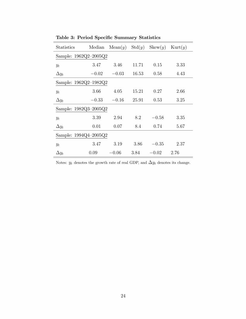
Table 3: Period Speci�c Summary Statistics
Statistics Median Mean(y) Std(y) Skew(y) Kurt(y)
Sample: 1962Q2�2005Q2
yt 3:47 3:46 11:71 0:15 3:33
�yt �0:02 �0:03 16:53 0:58 4:43
Sample: 1962Q2�1982Q2
yt 3:66 4:05 15:21 0:27 2:66
�yt �0:33 �0:16 25:91 0:53 3:25
Sample: 1982Q3�2005Q2
yt 3:39 2:94 8:2 �0:58 3:35
�yt 0:01 0:07 8:4 0:74 5:67
Sample: 1994Q4�2005Q2
yt 3:47 3:19 3:86 �0:35 2:37
�yt 0:09 �0:06 3:84 �0:02 2:76
Notes: yt denotes the growth rate of real GDP, and �yt denotes its change.
24

Table 4: Parameter Estimates for 2-Regime
Markov-Switching Models
Parameter MSI MSIH MSM MSMH
p1;1 0.98 0.99 0.98 0.99
p2;2 0.81 0.76 0.77 0.81
�1 3.38 3.23 3.91 3.68
�2 -1.78 -3.04 -2.14 -3.29
�1 0.14 0.16 0.14 0.22
�1 2.98 3.03 2.97 3.13
�2 2.98 0.97 2.97 0.71
Notes: 1 refers to the expansionary state, and 2 to the contractionary
state. The p�s are the transition probabilities de�ned in p. 11.
25
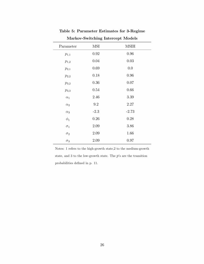
Table 5: Parameter Estimates for 3-Regime
Markov-Switching Intercept Models
Parameter MSI MSIH
p1;1 0.92 0.96
p1;2 0.04 0.03
p2;1 0.69 0.0
p2;2 0.18 0.96
p3;2 0.36 0.07
p3;3 0.54 0.66
�1 2.46 3.39
�2 9.2 2.27
�3 -2.3 -2.73
�1 0.26 0.28
�1 2.09 3.86
�2 2.09 1.66
�3 2.09 0.97
Notes: 1 refers to the high-growth state,2 to the medium-growth
state, and 3 to the low-growth state. The p�s are the transition
probabilities de�ned in p. 11.
26

Table 6: Business-Cycle Metrics for Linear Univariate and Multivariate Models
Metric / Model Actual RWD AR(1) VAR(2)
Duration (in quarters)
expansion
recession
4.0
40.25
2.47
37.68
2.8
28.0
2.96
29.3
Amplitude
expansion
recession
-0.03
0.4
-0.01
0.35
-0.01
0.03
-0.01
0.29
Cumulative
expansion
recession
-0.08
12.32
-0.02
11.39
-0.03
7.1
-0.03
7.45
Excess
expansion
recession
1.07
9.39
0.16
0.37
0.94
0.04
-0.55
-0.18
Coef. of variation of duration
expansion
recession
0.5
0.76
0.23
0.8
0.35
0.82
0.37
0.78
Coef. of variation of amplitude
expansion
recession
-0.84
0.81
-0.57
0.8
-0.64
0.85
-0.85
0.8
Occurrence of negative growth 13.3 16.2 16.7 16.3
Number of recessions 3 3.9 5.5 5.2
Std. dev. of output growth 3.42 3.46 3.43 3.5
Skew. of output growth 0.15 0.0 0.01 0.0
Kurt. of output growth 3.33 2.97 2.95 2.96
Skew. of the change in growth 0.59 0.0 0.01 0.0
Kurt. of the change in growth 4.48 2.97 2.97 2.95
Notes: All metrics are de�ned on p. 13. Bold items denote metrics for which the value calculated using
actual data is less (more) than the 10th (90th) percentile.
27

Table 7: Business-Cycle Metrics for Markov-Switching Models
Metric / Model Actual MSI2 MSIH2 MSI3 MSIH3 MSM2 MSMH2
Duration (in quarters)
expansion
recession
4.0
40.25
4.13
33.97
3.48
37.83
8.49
11.01
16.96
26.66
4.39
41.67
5.09
46.74
Amplitude
expansion
recession
-0.03
0.4
-0.2
0.34
-0.02
0.38
-0.06
0.11
-0.15
0.27
-0.03
0.47
-0.05
0.55
Cumulative
expansion
recession
-0.08
12.32
-0.09
10.24
-0.08
12.35
-0.45
1.22
-3.04
5.9
-0.12
16.53
-0.26
20.96
Excess
expansion
recession
1.07
9.39
-0.01
-0.31
-1.75
-0.68
-4.37
5.08
-2.28
-4.16
-0.29
0.34
-0.34
0.33
Coef. of variation of duration
expansion
recession
0.5
0.76
0.55
0.84
0.46
0.8
0.76
0.95
0.09
0.76
0.5
0.81
0.55
0.79
Coef. of variation of amplitude
expansion
recession
-0.84
0.81
-0.82
0.87
-0.83
0.82
-0.83
0.89
-1.05
0.76
-0.71
0.83
-0.83
0.79
Occurrence of negative growth 13.3 16.3 14.8 47.0 40.5 13.5 13.8
Number of recessions 3 4.3 3.8 8.8 3.9 3.3 2.8
Std. dev. of output growth 3.42 3.44 3.32 4.63 4.32 3.59 3.78
Skew. of output growth 0.15 -0.26 -0.12 0.55 0.34 -0.43 -0.35
Kurt. of output growth 3.33 3.15 2.86 2.94 2.65 3.47 2.98
Skew. of the change in growth 0.59 0.0 0.01 0.18 0.0 0.0 0.01
Kurt. of the change in growth 4.48 3.01 3.02 4.17 5.26 3.14 3.22
Notes: All metrics are de�ned on p. 13. Bold items denote metrics for which the value calculated using actual data
is less (more) than the 10th (90th) percentile.
28

Figure 1: Logarithm of Real Canadian GDP (top), Growth (middle), and Changein Growth (bottom)
29

Figure 2: Gain Curve of Expansions
30

Figure 3: Conditional Densities: Expansion vs. Contraction
31

Figure 4: Mixture of Densities (Notes: the solid line is the unconditional density ofCanadian GDP growth while long and short dashed lines are probability weighted conditionalexpansion and contraction densities, respectively. The mixing weight, �; is described inSection 3.1.)
32


