This article is the second in a series whose aim is to study existence, uniqueness and regular-ity of solutions of the Cauchy problem for the homogeneous (real and complex) Monge–Ampèreequation (HRMA/HCMA). The main result of the present article (Theorem 1) is that the well-known Legendre transform method for linearizing the HRMA fails to solve the equation, in evena weak sense, as soon as the solution develops singularities, or equivalently, as soon as the solu-tion of the linear equation fails to be convex. That is, the Monge–Ampère mass of the Legendretransform ‘solution’ becomes positive after this loss of convexity. At the same time, we showthat it does solve the equation on its dense regular locus, and we derive an explicit a priori upperbound on this mass. The proof of Theorem 1 uses tools of convex analysis and is independentof the quantum techniques of [27]. An important part of the analysis is to determine rather pre-cise regularity estimates for this function. This is achieved by establishing partial regularity forLegendre transforms of families of non-convex functions.
To put this result into context, we recall that the Cauchy problem studied in this article cor-responds to the initial value problem (IVP) for geodesics in the infinite dimensional space Hof Kähler metrics in a fixed class with the Riemannian metric defined by Mabuchi, Semmes,and Donaldson [19,31,4]. That is, the IVP for the geodesic equation is equivalent to a Cauchyproblem for the HCMA on the product ST × M of a strip, ST := [0, T ] × R, and a Kähler man-ifold M . As explained in more detail in [27], H is formally a symmetric space of non-positivecurvature and the behavior of its exponential map is related to several important conjectures inKähler geometry. The results of this article concern Kähler manifolds with torus symmetry (e.g.,toric or Abelian varieties) and to the flat, totally geodesic submanifold of torus-invariant metricsin H. In this case, the HCMA reduces to the HRMA on [0, T ] × R
n. Theorem 1 shows that formost initial directions, the “Legendre transform” curve ceases to be a geodesic (even in a weaksense) as soon as it develops singularities, but that it does solve the equation on its dense regular
Y.A. Rubinstein, S. Zelditch / Advances in Mathematics 228 (2011) 2989–3025 2991
locus. It is possible, but appears unlikely to us, that there exists an alternative definition of weaksolution which extends the solution to later times (or into the singular locus of the Legendre‘subgeodesic’) or that geodesics exist for longer times in less symmetric directions. Indeed, inthe first part [27], we constructed a general quantum analytic continuation potential on any pro-jective Kähler manifold M and conjectured that it solved the IVP for as long as a solution exists.In the torus-invariant case, we showed that it equals the Legendre transform potential. Hence theresults of this article cast serious doubt on the existence of weak geodesics rays through mostsmooth initial directions. We discuss the possibilities further after stating our results.
The Cauchy problem for HRMA studied in this article is given by
MAψ = 0, on [0, T ] × Rn,
ψ(0, · ) = ψ0( · ), on Rn,
∂ψ
∂s(0, · ) = ψ0( · ), on R
n. (1)
Here, MA denotes the real Monge–Ampère operator that associates a Borel measure to a convexfunction (see Section 2.2) and equals det∇2ψ dx1 ∧· · ·∧dxn+1 on C2 functions. For the Cauchydata we require that ψ0 be smooth, strictly convex with invertible Hessian, and of linear growthon R
n, and that ψ0 be bounded and smooth on Rn.
It is well known that the HRMA is linearized by the Legendre transform. In geometric terms,the Legendre transform is an isometry between the space of open-orbit Kähler potentials and thespace of symplectic potentials. Both spaces are flat, however the latter also has a trivial connec-tion (see [26, §3]). Therefore, a geodesic {ψs} of open-orbit Kähler potentials, i.e., a solution of(1) with ψs = ψ(s, · ), is transformed under the Legendre transform to a straight line of sym-plectic potentials
ψ�s = us = u0 + su0 (2)
where
u0 := ψ�0 , u0 := −ψ0 ◦ (∇ψ0)
−1,
are defined on the polytope P = Im∇ψs corresponding to the toric Kähler class (see Section 2.3for more background, as well as [26, §3], and [27, §§4.2]). There exists a certain (typically)finite time T cvx
span, that we call the convex lifespan, such that (1) restricted to [0, T cvxspan) × R
n maybe linearized and hence solved via the Legendre transform. One has
T cvxspan(ψ0, ψ0) := sup
{s: ψ�
0 − sψ0 ◦ (∇ψ0)−1 is convex on Im∇ψ0
}. (3)
The corresponding solution, that we call the Legendre transform potential, can be written explic-itly as,
The standard proofs that ψ solves the HRMA when us = u(s, · ) solves the linear equationu = 0, break down as soon as ψ is not twice differentiable, or equivalently when us ceases to beconvex. The underlying reason is that the Legendre transform is not a bijection on non-convex
2992 Y.A. Rubinstein, S. Zelditch / Advances in Mathematics 228 (2011) 2989–3025
functions. Nevertheless it is possible that ψ solves HRMA even for T > T cvxspan in a weak sense.
As explained in Section 10, ψ is convex in (s, x) and therefore is always a subsolution of (1).The main result of this article is that ψ does not solve the HRMA (1) for any T > T cvx
span,even in a weak sense. At the same time, we prove that ψ does solve the equation wherever it isdifferentiable, and in particular on a dense set whose complement has zero Lebesgue measure.To state our result, let
�(ψ) := {(s, x): ψ is finite and differentiable at (s, x)
} ⊂ R+ × Rn, (5)
denote the regular locus of ψ . Similarly, we denote the regular locus of ψs (i.e., where ψs isdifferentiable as a function of x alone) by �(ψs) ⊂ R
n. Let
Σsing := R+ × Rn \ �(ψ),
denote the singular locus of ψ , and set
Σsing(T ) := Σsing ∩ [0, T ] × Rn.
Since ψ is everywhere finite the singular locus of ψ has Lebesgue measure zero, and the regularlocus is dense in R+ × R
n.
Theorem 1. Let ψ be defined by (4) for all (s, x) ∈ R+ × Rn. Then
(i) ψ solves the HRMA (1) on the regular locus. Namely,
MAψ = 0 on �(ψ).
In addition, [0, T cvxspan) × R
n ⊂ �(ψ).(ii) Whenever T > T cvx
span, ψ fails to solve the HRMA (1). In particular, the Monge–Ampère mea-sure of ψ charges the set Σsing(T ) with positive mass and we have,
∫[0,T ]×Rn
MAψ =∫
Σsing(T )
MAψ > 0.
Before sketching the proof, we briefly continue the discussion at the start of the introductionabout the implications of Theorem 1 for the general question of defining weak geodesic rays inthe space of Kähler metrics.
The results suggest that there do not exist even weak geodesic rays in the space of Kählermetrics for most smooth initial directions, and it raises the question of characterizing initial di-rections of rays on general Kähler manifolds. But it leaves open the possibility that there existssome other notion of weak solution besides the Legendre transform definition that might extendthe solution to later times or through the singular set of the Legendre transform potential. Thismight seem plausible at first if one considers that smooth solutions of the HRMA can be ex-pressed in terms of the initial data by the method of characteristics. Indeed, when φ ∈ C3 anddet∇2
s,xφ = 0, and when ∇2xφ(s, ·) is non-degenerate for each s, then ker∇2φ is a 1-dimensional
distribution whose characteristics are straight lines, and φ is linear along them [14,8]. Loss ofconvexity occurs when the characteristics intersect. Hence the situation is somewhat analogous
Y.A. Rubinstein, S. Zelditch / Advances in Mathematics 228 (2011) 2989–3025 2993
to conservation laws or Hamilton–Jacobi equations, and one might hope to define non-smoothweak solutions by some analogue of the Lax–Oleinik and Hopf–Lax formulas, whose definitionin fact involves the Legendre transform [6]. However, the fact that the HRMA is second orderinstead of first order makes this possibility seem dubious to us. The usual integration by partsargument used to define weak solutions for conservation laws breaks down when the equationis second order. As mentioned above, we previously proposed a general definition of a weaksolution by a quantization method and in the torus-invariant case it was shown to coincide withthe Legendre definition [27]. This, together with the fact that the Legendre transform definitionappears to be the closest analogue of the Lax–Oleinik and Hopf–Lax formulas, cast doubt on theexistence of an alternative (inequivalent) definition of weak solution. We pursue this further inthe sequels to this article, and build upon the partial regularity theory developed here in order tounderstand general weak solutions to the HRMA. In the apparent absence of global in time weaksolutions we also initiate a study of certain ‘optimal’ subsolutions, and among these the notionof a “leafwise subsolution” [28].
There do exist at least two other approaches to finding weak geodesic rays through a point ϕ0in H (see [27] for references). One is by constructing special degenerations or test configurationsusing the projective embeddings associated to ϕ0, and converting them into geodesic rays. Itappears that in most cases the test configuration method produces C1,1 geodesics, and thereforethe initial data ϕ0 ∈ Tϕ H would not be smooth (as we assume). Another approach is to connect ϕ0to a distant point ϕ1 by a geodesic, and move ϕ1 off to ‘infinity’. But again the known regularityresults for the end-point problem only ensure that the initial velocity ϕ0 is at best C0,1. It thereforeseems quite possible that, generically, geodesic rays exist mostly in singular directions.
1.1. Outline of the proof
Let us outline the main steps in the proof. In addition, a concrete overview of the proof isgiven in Section 3 for the case n = 1.
In order for a convex function to be a weak solution of the HRMA the image of its subdiffer-ential must be a set of Lebesgue measure zero. Our goal is therefore to obtain some descriptionof the subdifferential mapping ∂ψ . First, we study the regularity of the restriction ψs of ψ toeach time slice. Let
As := {y ∈ P : us(y) = u��
s (y)} ⊂ P. (6)
Proposition 1. For each s > 0, the function
ψs(x) := (u0 + su0)�(x), x ∈ R
n,
is a continuous strictly convex function on Rn. It is Lipschitz continuous but not everywhere
differentiable. The singular locus of ψs contains the set ∇u��s (As \ ∂P ).
Geometrically, Proposition 1 implies that ψ can be regarded as a ray in the space of Lipschitzcontinuous open-orbit Kähler potentials. Its proof is completed at the end of Section 10, and isdivided into several steps. We also remark that the strict convexity is not directly used for theproof of Theorem 1, however several of the ingredients in its derivation are.
2994 Y.A. Rubinstein, S. Zelditch / Advances in Mathematics 228 (2011) 2989–3025
First, in order to prove that ψs is strictly convex we study the regularity of its dual u��s . We
prove interior C1 regularity for u��s (Lemma 4.1). Then we prove that u��
s is moreover essentiallysmooth (Lemma 6.1), i.e., its gradient blows up on ∂P . These results, together with a classicalduality result, then imply the strict convexity of ψs . Here one uses the fact that ψs is everywherefinite, and so its subdifferential has domain equal to R
n, and also Im ∂u��s = R
n. These facts canbe seen directly for our explicit ψs , but we also include a different proof (Lemma 7.2) using ahomotopy argument that may have its own interest, and also shows as a by-product that u��
s and∇u��
s are continuous in s, a fact that is used later.Second, to show that ψs is not differentiable we show that u��
s is not strictly convex. To thatend, for each s > T cvx
span, we consider the set As ⊂ P defined in (6). We show that this set can bepartitioned into convex sets
As \ ∂P =⋃
v∈As
Q(s, v) ∩ As \ ∂P
along which ∇u��s is constant (Sections 9 and 13). Each such convex set Q(s, y) (see (62))
contains at least a line, proving that ψs is not differentiable at x. We then obtain an estimate onthe regular locus of ψs in terms of us and As (Lemmas 9.1 and 10.3), and this concludes theproof of Proposition 1.
The results above describe the singularities of each ψs . Next, we prove a partial C1 regularityresult for ψ (Lemma 10.4) that, as a corollary, gives a precise description of the singularities ofψ . Recall that �(f ) denotes the set on which f is finite and differentiable.
Proposition 2. Assume that x ∈ �(ψs). Then (s, x) ∈ �(ψ). I.e., the singular locus of ψ is the(indexed) union over s of the singular loci of the functions ψs . In terms of the regular loci,
�(ψ) =⋃s�0
{s} × �(ψs).
In other words, wherever ψ is differentiable in x it is also differentiable in s. The resultsdescribed so far then imply an alternative description for the regular locus �(ψ) in terms of themaps ∂us , s ∈ R+ (Proposition 10.1). This allows us to show that ψ solves the HRMA on theregular locus. In fact, the image of the (total) subdifferential of ψ evaluated on the regular locusis just the graph of −u0 over P \ ∂P , and this, as a set in R
n+1, has Lebesgue measure zero(Proposition 11.1).
To conclude the proof it thus remains to analyze the Monge–Ampère measure MAψ onthe singular locus. By using some elementary facts regarding partial subdifferentials of con-vex functions of several variables we obtain some lower and upper bounds on ∂ψ({s} × R
n)
(Lemma 12.4).
Lemma 1. Let y ∈ As \ ∂P , and let x := ∇u��s (y). Then
co{(−u0(v), v
): v ∈ γxψ(s, x)
} ⊂ ∂ψ(s, x) ⊂ co{(−u0(v), v
): v ∈ ∂xψ(s, x)
}.
These bounds are obtained in terms of certain convex sets projecting onto the pieces Q(s, v)
of the partition of As . Using these bounds, along with monotonicity and continuity of the familyof the one-parameter family of sets As (Lemmas 8.1 and 8.2), we show that the subdifferential
Y.A. Rubinstein, S. Zelditch / Advances in Mathematics 228 (2011) 2989–3025 2995
of ψ in fact “fills-in” a portion of the region lying between the graph of −u0 and the graphof minus the convexification of u0 (see Figs. 3 and 4), hence the mass of MAψ necessarilybecomes positive for any T > T cvx
span (Proposition 13.1 and Lemma 13.3), completing the proof ofTheorem 1.
Thus, perhaps the main new picture this article conveys is that when convexity is lost, theimage of the subdifferential is no longer confined to the graph of −u0 but rather to the openregion between this graph and that of its concavification. Possibly surprisingly, this indicates thatthe exponential map of the flat space of toric Kähler metrics does not exist for all time.
It is worth pointing out that the proof also shows that the Monge–Ampère mass of ψ has ana priori upper bound depending only on the Cauchy data (Lemma 13.3). Let epif denote theepigraph of f (see Section 2.1).
Proposition 3. Let T > 0. One has,
∫[0,T ]×Rn
MAψ � Vol(epi(−u0) \ epi
(−(u0)��
)),
where the right-hand side denotes the Euclidean volume in Rn+1 of the set of points lying below
the graph of u0 and above the graph of its convexification, over P .
The graph of ψ defines a hypersurface in Rn+2 that is Gauss flat over [0, T cvx
span) × Rn. Propo-
sition 3 implies that the non-compact hypersurface in Rn+2 defined by the graph of ψ over
[0, T ] × Rn, while not flat, has finite total Gauss curvature (see Sections 1.4 and 3).
Note that the right-hand side is zero if and only if u0 is convex, thus T cvxspan = ∞. The inequality
is also optimal when the right-hand side is positive. This can be seen by considering, for instance,explicit examples in n = 1 (see Section 3), where equality is attained in the limit where T tendsto infinity.
It is interesting to give a geometric description of the singular locus Σsing on which theMonge–Ampère mass is concentrated. By Propositions 1 and 2 we have an explicit descriptionof the singular locus (assuming the Cauchy data (u0, u0) is generic),
Σsing =⋃
s�T cvxspan
{s} × ∇u��s (As \ ∂P ). (7)
Now, by the continuity of ∇u��s in s and the set-valued continuity of the sets As , it follows
that Σsing is a countable union of C0 hypersurfaces in Rn+1. Moreover, by general results of
Alberti [1] in fact Σsing must be a countable union of locally Lipschitz continuous hypersurfacesin R
n+1. Further, for reasonable Cauchy data, e.g., such that As has finitely many componentsfor all s > 0, it follows from (7) that Σsing will also be composed of finitely many hypersurfaces.A visualization of the singular set and the corresponding ‘corner set’ of the graph of ψ is givenin Section 3 (see Figs. 2 and 3).
1.2. Examples on S2
We illustrate with an example the behavior of the family of Kähler metrics (viewed as a pathin H) associated with the quantum analytic continuation (or Legendre transform) potential.
2996 Y.A. Rubinstein, S. Zelditch / Advances in Mathematics 228 (2011) 2989–3025
Let (P1,ω) denote the Riemann sphere equipped with a Kähler form ω. Consider an S1-invariant Kähler metric ωϕ0 on P
1 that equals√−1∂∂ψ0 away from the poles. Let ϕ0 denote a
given S1 invariant initial velocity. The geodesic equation
∂2ψ
∂s2=
(∂2ψ
∂x2
)−1(∂2ψ
∂x∂s
)2
, (8)
can be interpreted as the HRMA det∇2ψ = 0. Denote
ψ ′(s, x) := ∂ψ(s, x)
∂x, ψ(s, x) := ∂ψ(s, x)
∂s.
By letting y := ψ ′(s, x), and u(ψ ′(s, x)) := xψ ′(s, x) − ψ(s, x), a computation shows thatEq. (8) becomes u(s, y) = 0, solved by u(s, y):= u0(y)+su0(y), with u0(y) = −ψ0((ψ
′0)
−1(y)).Note that y = ys, θ are the action-angle variables for ωs = √−1∂∂ψ(s, x), i.e. ωs = dys ∧dθ
and ys is the moment map of the S1 action with respect to ωs . Let z = ex+√−1θ denote theholomorphic coordinate away from the poles. The metric gs at time s is then given by
gs = ψ ′′(s, x)(dx2 + dθ2), (9)
expressed in action-angle variables as
gs = u(s)yydy2 + 1
u(s)yy
dθ2, (10)
where u(s)yy denotes the second derivative of the symplectic potential u at time s with respectto the action variable y = ys . Also, let rs denote the geodesic distance function from the northpole (the fixed point of the S1 action on which ys takes its maximum). Then rs is a function onlyof ys . Hence the change of variables from ys to rs does not add any term containing dθ , and
gs = dr2s + 1
u(s)yy
dθ2. (11)
Formulas (10)–(11) are valid only as long as u(s, · ) = u0 + su0 remains convex, and theyshow that in that regime gs is a smooth metric. The Legendre transform potential ψ definedby (4) provides an extension of the path of metrics {gs}s∈[0,T cvx
span)given by (10) to s ∈ [T cvx
span,∞),given by
gs = u�s′′(s, x)
(dx2 + dθ2). (12)
Eq. (4) also means that ψ(s, · ) is the Legendre dual of the convexification of u(s, · ). The con-vexified symplectic potential u��
s is C1 but develops straight segments on some intervals (seeFig. 1). At these, u��(s)yy = 0. Thus, the metric develops an S1-invariant delta-function singu-larity at the corresponding value of rs . Theorem 1 is the statement that the path of metrics gs
ceases to be a geodesic precisely at T cvxspan, when the singularities appear. However, it does satisfy
the geodesic equation on a dense set, whose time slice is the complement of a discrete set ofsingular S1 orbits.
Y.A. Rubinstein, S. Zelditch / Advances in Mathematics 228 (2011) 2989–3025 2997
Fig. 1. The graphs of us and u��s over P for s > T cvx
span.
1.3. Asymptotic behavior of geodesic and subgeodesic rays
It has been conjectured by Donaldson that smooth geodesic rays in the space of Kähler met-rics should play an important role in questions regarding geometric ‘stability’ and existence ofcanonical metrics [4]. An important question is therefore precisely which directions yield smoothgeodesic rays. We prove in the sequel that for the HRMA (1) one has T ∞
span = T cvxspan [28], i.e., the
lifespan of a smooth solution, is equal to the convex lifespan (the notation follows that of [27]).Therefore the directions of smooth toric geodesic rays are precisely those with infinite convexlifespan, or, in other words, with u0 smooth and convex. Further, as a corollary of the results hereand in the sequel we obtain a description of the limiting behavior of the rays obtained by solvingthe IVP using the quantum method of [27], or, equivalently, by means of the Legendre transformmethod. This holds whether they be smooth geodesics or only ‘subgeodesics’, by which we meansubsolutions of the HCMA.
1.4. Other Cauchy problems for the HRMA
The IVP for geodesics in the space of toric metrics on toric varieties gives rise to a specificCauchy problem for the HRMA. A natural question is to what extent do the techniques usedin this article generalize to other Cauchy problems for the HRMA. We briefly discuss severalpossible problems and generalizations, some of which we hope to discuss in more detail else-where.
Aside from the fact that the Cauchy data and the Cauchy hypersurface are smooth, and thatwe require all solutions to be convex, the main distinctive features of the Cauchy problem (1)are:
(i) the Cauchy hypersurface is an Rn-slice of the total space [0, T ] × R
n,(ii) the initial convex function has linear growth at infinity, and the initial velocity is uniformly
bounded.
An example of a Cauchy problem where (i), but not (ii), holds, is the IVP for geodesics in thespace of toric metrics on Abelian varieties. In that setting the convex function ψ0 has quadraticgrowth at infinity. On the other hand, the gradient map ∇ψ0 now maps to a torus instead of apolytope. It follows that the symplectic potential ψ�
0 can be considered as a convex function onR
n with quadratic growth and no singularities. This fact eliminates the need for the analysis nearthe boundary of P that was necessary in this article. Although we do not go into the details here,
2998 Y.A. Rubinstein, S. Zelditch / Advances in Mathematics 228 (2011) 2989–3025
using the methods of this series one may prove an analogue of our main results for this class ofmanifolds.
Note that the requirement in (ii) that the initial velocity be bounded, while the initial convexfunction divergent at infinity, guarantees that the gradient image of ψs remains constant, and thisstill held true in the Abelian case. Removing this assumption from (ii) would require dealingwith a one-parameter family of gradient images Ps , and would certainly complicate some of theanalysis.
Next, one may allow the Cauchy hypersurface to be more general, for example a smooth affinehypersurface in an affine manifold. Geometrically, this setting arises when one considers the IVPfor geodesics in spaces of invariant metrics in various classes of manifolds with large symmetrygroups (for examples see, e.g., [5, §4]). It would be interesting to obtain a formula for T ∞
spananalogous to the one for the convex lifespan (3). We note that in the affine setting Foote [8,9] hasgiven a sufficient condition on the Cauchy data and hypersurface to have T ∞
span > 0.Although the affine situation is certainly more complicated than the Euclidean one it seems
plausible to us that one could generalize at least some of the techniques of the present series tothe affine setting.
Finally, we mention that the Cauchy problem for the HRMA is also classically used to con-struct smooth Gauss flat hypersurfaces in R
n+2 (this is carried out in R3 in [33,29]; a classical
reference on flat surfaces is Pogorelov [22]). It seems interesting to investigate what kind of sin-gular hypersurfaces are obtained from the Legendre transform method when extended beyondthe convex lifespan. A consequence of the a priori bound of Proposition 3 is that the resultinghypersurface has bounded total Gauss curvature, a fact that might seem rather surprising at first.In Section 3 we briefly touch upon this point of view by sketching the proof of Theorem 1 in thecase n = 1, and also illustrate explicitly the finite curvature phenomenon.
2. Background
In this section, we recall some basic definitions relating to convex analysis, the real Monge–Ampère operator, and the reduction of HCMA on toric Kähler manifolds to the HRMA. Foradditional necessary notation and definitions that are used throughout we refer to [27, §§4.3].
2.1. Convex analysis
For general background on Legendre duality and convexity we refer the reader to [16,17,24],whose notation and terminology we largely adhere to. Denote by intA the interior of a set A, andby
coA
its convex hull. Given a function f defined on a set P ⊂ Rn let
epif := {(x, r): r � f (x), x ∈ P
}denote its epigraph. A vector v ∈ (Rn)� is said to be a subgradient of a function f at a point x iff (z) � f (x)+〈v, z−x〉 for all z. The set of all subgradients of f at x is called the subdifferentialof f at x, denoted ∂f (x).
Y.A. Rubinstein, S. Zelditch / Advances in Mathematics 228 (2011) 2989–3025 2999
The Legendre–Mandelbrojt–Fenchel conjugate of a continuous function f = f (x) on Rn is
defined by [20,7]
f �(y) := supx∈Rn
(〈x, y〉 − f (x)).
For simplicity, we will refer to f � sometimes as the Legendre dual, or just dual, of f .
Definition 2.1. A convex function f is called proper if it is not identically +∞ and is uniformlybounded below. A proper convex function is called closed if it is lower semi-continuous. Thedomain of ∂f is defined by dom(∂f ) := {x: ∂f (x) = ∅}.
(i) A function on a convex set C is called strictly convex on C if for every λ ∈ (0,1) and alldistinct points x1, x2 ∈ C holds f ((1 − λ)x1 + λx2) < (1 − λ)f (x1) + λf (x2).
(ii) A proper convex function is called essentially strictly convex if it is strictly convex on everyconvex subset of dom(∂f ).
(iii) A proper convex function is called essentially smooth if C := int(dom(∂f )) = ∅, if f isdifferentiable on C and if limi→∞ |∇f (xi)| = +∞ whenever {xi}i�1 is a sequence in C
converging to x ∈ ∂C.
2.2. The real Monge–Ampère operator
We recall the definition of the Monge–Ampère operator and its basic characterization, due toAlexandrov and Rauch–Taylor. Let M(Rn+1) denote the space of differential forms of degreen+ 1 on R
n+1 whose coefficients are Borel measures (i.e., currents of degree n+ 1 and order 0).
Proposition 2.2. (See [23, Proposition 3.1].) Define by
MAf := d∂f
∂x1∧ · · · ∧ d
∂f
∂xn+1,
an operator MA : C2(Rn+1) → M(Rn+1). Then MA has a unique extension to a continuousoperator on the cone of convex functions.
An alternative, geometric, definition is due to Alexandrov, and uses the notion of a subdiffer-ential of a convex function.
Proposition 2.3. (See [23, Section 2].) For any convex function f , the measure M A f , definedby
(M A f )(E) := Lebesgue measure of ∂f (E),
is a Borel measure.
The following result links these two definitions and will be crucial below.
3000 Y.A. Rubinstein, S. Zelditch / Advances in Mathematics 228 (2011) 2989–3025
Theorem 2.4. (See [23, Proposition 3.4].) For every convex function f on Rn+1 one has the
equality of Borel measures MAf = M A f . In particular, the real Monge–Ampère measure iszero if and only if the image of the subdifferential map has Lebesgue measure zero in R
n+1.
2.3. The Cauchy problem for the symplectic potential
It is well known that the Legendre transform linearizes the HRMA [14,30]. This fact also hasan infinite dimensional geometric interpretation that we now briefly review.
Let (M,ω) be a toric Kähler manifold of complex dimension n and let T = (S1)n denotethe real torus of dimension n which acts on (M,ω) in a Hamiltonian fashion. We denote byH(T) the class of T-invariant Kähler metrics in the cohomology class of ω. On the open-orbit ofTC = (C�)n, a T-invariant Kähler metric has a Kähler potential ψ and we also write ψ ∈ H(T).
Since it is T-invariant, the Kähler potential may be identified with a smooth strictly convexfunction on R
n in logarithmic coordinates. Therefore its gradient ∇ψ is one-to-one onto theconvex polytope P = Im∇ψ and one has the following explicit expression for its Legendre dual,
u(y) = ψ�(y) = ⟨y, (∇ψ)−1(y)
⟩ − ψ ◦ (∇ψ)−1(y), (13)
which is a smooth strictly convex function on P , satisfying
∇u(y) = (∇ψ)−1(y), (14)
and
(∇2u(y))−1 = ∇2ψ
((∇ψ)−1(y)
)(15)
([24], or [25, pp. 84–87]). Following Guillemin, the function u is called the symplectic potentialof the metric
√−1∂∂ψ . The space of all symplectic potentials is denoted by L H(T). Put
uG :=d∑
k=1
lk log lk, (16)
where lk are the defining linear functionals of the polytope P (we refer to [27, §§4.2] for nota-tion). A result of Guillemin [12] states that for any symplectic potential u the difference u − uG
is a smooth function on P (that is, up to the boundary). In other words,
L H(T) = {u ∈ C∞(P \ ∂P ): u = uG + F, with F ∈ C∞(P )
}. (17)
The Legendre transform is an isometry between (H(T), gL2) and (L H(T),L2(P )). It trans-forms the Christoffel symbols of (H(T), gL2) to zero and thus linearizes the Monge–Ampèreequation to the equation u = 0 (for more on this see [30,11], or [26, §3]). The differential of theLegendre transform acts as minus the identity, that is, if ηs is a curve in H(T) and if us := η�
s arethe corresponding symplectic potentials then
ηs = −us ◦ ∇ηs (18)
Y.A. Rubinstein, S. Zelditch / Advances in Mathematics 228 (2011) 2989–3025 3001
(see, e.g., [25, p. 85]). Therefore the IVP on (H(T), gL2) is transformed to the following initialvalue problem for geodesics in the space of symplectic potentials:
u = 0, u0 = ψ�0 , u0 = −ψ0 ◦ (∇ψ0)
−1. (19)
3. Legendre continuation of flat surfaces in RRR3
Our purpose in this section is to explain the proof of Theorem 1 in the case where n = 1,i.e., for the Cauchy problem for the 2-dimensional HRMA of Section 1.2. This special setting issimpler to visualize explicitly and helps motivate and better capture some of the constructionscarried out in the proof of Theorem 1, and also, part of the analysis simplifies. Many of theassertions in this section are stated without rigorous justification, and their proofs can be found(for all n) in later sections.
The graph of ψ(s, x)
{(s, x,ψ(s, x)
)} ⊂ R3
over [0, T cvxspan] × R is a flat surface since its second fundamental form is proportional to the
Hessian of ψ . We are interested in what happens to this surface when extended beyond T cvxspan:
does ψ still define a flat surface, in a weak sense, after T cvxspan?
Let ωFS denote the Fubini–Study form of constant Ricci curvature 1 on the Riemann sphere,given locally by
ωFS =√−1
π
dz ∧ dz
(1 + |z|2)2.
The associated open-orbit Kähler potential can be taken as
ψ0(x) = log(1 + |z|2) − 1
2Re z = log
(1 + e2x
) − x. (20)
The corresponding moment polytope is [−1,1], and the symplectic potential dual to ψ0 can becomputed via the moment map y(x) = ψ ′
We start with the analysis of u��s . By (21) we have limy→±1 u′
0 = ±∞, and the same holds forus since u0 is bounded on P . Therefore, when restricted to a neighborhood of {±1} in [−1,1] thetangent lines to the graph of us lie below the graph. Hence, As ∩ {±1} = ∅, and the graphs of us
and of u��s differ only above (−1 + ε,1 − ε) for some ε > 0. Above every connected component
of As the graph of u��s is necessarily affine with slope precisely equal to the derivative of us at
the end-points. Hence u�� is continuously differentiable in P \ ∂P (and even C1,1).
s
3002 Y.A. Rubinstein, S. Zelditch / Advances in Mathematics 228 (2011) 2989–3025
Let s > T cvxspan so As = ∅. Let us assume for simplicity that As is connected, with As =
(as, bs) ⊂ [−1,1], and that u��s is nowhere affine outside of As . Set xs := ∇u��
s ((as, bs)).Then the graph of ψs has a corner of angle αs = tan−1 as − tan−1 bs at (xs,ψs(xs)),and is smooth elsewhere. The set of reachable subgradients of ψs at xs is γψs(xs) ={as, bs}. It follows that γψ(s, xs), the set of reachable subgradients of ψ at (s, xs), contains{(−u0(as), as), (−u0(bs), bs)}. Thus, by convexity, the total subdifferential of ψ at (s, xs) con-tains the line connecting these two points:
co{(−u0(as), as
),(−u0(bs), bs
)} ⊂ ∂ψ(s, xs). (22)
On the other hand, the graph of −u0 cannot be linear on (as, bs) since that would implythat u0 + su0 were strictly convex on (as, bs). It follows that the affine segment in (22) doesnot intersect the graph of −u0 over (as, bs) at least above some open subset of (as, bs). SinceAs is monotonically increasing in s in a continuous fashion, we conclude that the image of ∂ψ
fills-in a region in R × [−1,1] above the graph of −u0, and consequently that ψ is not a weaksolution of the 2-dimensional HRMA on [0, T ] × R for any T > T cvx
span. Moreover, the regionfilled out, as T tends to infinity, is contained in the region above the graph of −u0 and below thegraph of −(u0)
��. We conclude that the non-compact surface defined by ψ is flat precisely onthe complement of the corner set, but not globally flat. However, its total curvature in the senseof Alexandrov while positive, is finite, and is concentrated on the codimension one corner set.
Example 3.1. The graph of ψ may be parametrized with respect to the moment coordinate onthe domain of its invertibility, namely,
graph of ψ = {(s,∇us(y),
⟨y,∇us(y)
⟩ − us(y)): s ∈ R+, y ∈ P \ (As ∪ ∂P )
}.
To visualize the graph of ψ in a specific example let ψ0 be given by (20), and set
ϕ0(z) =( |z|2 − 1
|z|2 + 1
)2
, or ψ0(x) =(
e2x − 1
e2x + 1
)2
. (23)
Hence, u0(y) = −y2.A portion of this graph is drawn in Fig. 2. In this example, T cvx
span(ψ0, ψ0) = 1, and the graphof ψ develops a kink along the corner set above Σsing = {x = 0, s > 1}. For each s > 1 the graphof ψs has a kink at x = 0, and so the corner set of ψ is precisely the union over s of the cornersets of ψs . Moreover, in this special example u0 and u0 are even functions. The same is thentrue for ψs , and one may further show that ψ is differentiable in s. Let As = (−as, as). Then∂xψ(s, xs) = [−as, as], and
∂ψ(s, xs) = {ψs(xs)
} × ∂xψ(s, xs) = {(a2s , y
): y ∈ [−as, as]
}.
A typical set of the form ∂ψ([0, T ] × Rn) is illustrated in Fig. 3. It is contained in the set
epi(−u0) \ epi(−(u0)��), with (u0)
��(y) ≡ −1. The total curvature of graph(ψ) is boundedfrom above by the area of the difference between the epigraph of −u0 and that of −(u0)
��
Y.A. Rubinstein, S. Zelditch / Advances in Mathematics 228 (2011) 2989–3025 3003
Fig. 2. The graph of ψ for (s, x) ∈ [0,2] × [−3,3] and Cauchy data (ψ0, ψ0) given by (20) and (23).
Fig. 3. The dotted and shaded region is ∂ψ([0,1.5] × R) for the Cauchy data (ψ0, ψ0) given by (20) and (23).
(over [−1,1]),
∞∫0
∞∫−∞
MAψ =1∫
−1
(1 − y2)dy = 4
3.
Indeed, the total curvature is given by the measure in Sn of the unit normals to the surface, that isdominated from above by the Lebesgue measure of its stereographic projection in R
n. The latteris precisely the Monge–Ampère mass (see [23, Proposition 2.3], or [22]). Thus, while the surface
3004 Y.A. Rubinstein, S. Zelditch / Advances in Mathematics 228 (2011) 2989–3025
has an infinitely long corner set, the surface quickly becomes ‘almost linear’ outside it, and in amanner guaranteeing its total curvature remains finite.
4. Interior C1 regularity of u��s
The purpose of this section is to prove Lemma 4.1, which shows that u��s is C1 on the interior
of P .Let f ∈ C0(P ). The biconjugate f �� of f is a convex function on P and can be characterized
as the ‘convex envelope’ of f [17, Theorem 1.3.5, p. 45]
f ��(x) = sup{g(x): g convex on P and g � f
}= sup
{a(x): a affine on P and a � f
}. (24)
Consider a smooth function defined on a compact convex set and smooth in its interior. It is nottrue in general that its biconjugate is differentiable in the interior. However, in our situation thebiconjugate enjoys the maximal degree of regularity possible in general, i.e., it is C1,1 (no gain isachieved by considering a real-analytic function). General results in the literature (see [2,10,18]and [17, §X.1.5]) are usually stated for functions defined on all of R
n that obey certain growthconditions at infinity (cf. [10, (2.3)], [17, (1.5.2), p. 50], [2, (18)], [18, (1)]) or else make certainassumptions regarding boundary behavior that need not hold in our situation (cf. [10, (4.1)] andparticularly [10, Remark 4.3]). For these reasons, and since the constructions involved will beuseful later, we find it beneficial to extract from the references above partially self-containedproofs of differentiability of u��
s . The C1,1 estimate can be deduced from the C1 estimate, but wewill not need that here.
Lemma 4.1. Let s > 0.
(i) The graph of the Legendre double dual of us is the lower boundary of the closed convex hullof the epigraph of us .
(ii) u��s ∈ C1(P \ ∂P ) ∩ C0(P ).
Proof. (i) From (24) it follows that for any finite convex function f defined on P , one has
co epif = epif ��. (25)
Since us is smooth and continuous up to the boundary of P the convex hull of epius is closed,and the result follows.
(ii) From (24) we have u��s � us . Since us majorizes a linear function on P it also follows that
u��s is bounded below. Hence u��
s ∈ C0(P ).We divide the proof of the C1 estimate into two steps and closely follow [2,17]. The proof
will show that for any compact subset Ω ⊂ P \ ∂P there exists a compact subset Ω ′ ⊂ P \ ∂P
with Ω ⊂ Ω ′ such that
∥∥∇u��s
∥∥C0(Ω)
� ‖∇us‖C0(Ω ′) < C(s + 1),
with C = C(Ω,Ω ′, u0, u0) > 0.
Y.A. Rubinstein, S. Zelditch / Advances in Mathematics 228 (2011) 2989–3025 3005
First step. Denote by �n+1 ⊂ Rn+1 the unit simplex
�n+1 :={
λ = (λ1, . . . , λn+1) ∈ Rn+1: λi � 0,
n+1∑i=1
λi = 1
}.
Recall the following representation formula for the biconjugate function [24, Corollary 17.1.5],
u��s (y) = inf
{λ · (us(y1), . . . , us(yn+1)
): λ ∈ �n+1, yi ∈ P,
n+1∑i=1
λiyi = y
}. (26)
We claim that there exist—for each y ∈ P \ ∂P —points y1, . . . , yn+1 ∈ P and a vector λ ∈ �n+1such that
(y,u��
s (y)) =
n+1∑i=1
λi
(yi, us(yi)
). (27)
To see that, observe that according to (i) the epigraph of u��s is the closed convex hull of the
epigraph of us . Hence, by convexity, for each y ∈ P \ ∂P there exists an m ∈ N and a λ ∈ �m
and {(yi, ri)}mi=1 ⊂ epius such that
(y,u��
s (y)) =
m∑i=1
λi(yi, ri). (28)
But then since us(yi) � ri , and∑m
i=1 λi(yi, us(yi)) also belongs to epius it follows that when-ever λi > 0 there holds ri = us(yi): otherwise (y,u��
s (y)) would lie “directly above” anotherpoint in the convex hull of epius , contradicting (i). Finally, using (i), since the convex hull of theepigraph of us is closed, it follows that (y,u��
s (y)) lies on its boundary; then by a consequenceof Carathéodory’s theorem it is possible to take m = n+ 1 in (28) [16, Proposition 4.2.3, p. 126].
Second step. When Eq. (27) holds, set
I := {i: λi > 0}. (29)
Following the terminology of [2, §3], we say that the points {yi}i∈I are called upon by y. Weomit from the notation the dependence of yi on y. By (24) u��
s is convex and u��s � us . Hence,
u��s (y) � λ · (u��
s (y1), . . . , u��s (yn+1)
)� λ · (us(y1), . . . , us(yn+1)
),
which together with (27) implies
u��s (yi) = us(yi), ∀i ∈ I. (30)
Claim 4.2. Let y ∈ P \ ∂P , and let {yi} and I be defined by (27) and (29), respectively. Then foreach i ∈ I one has yi ∈ P \ ∂P .
3006 Y.A. Rubinstein, S. Zelditch / Advances in Mathematics 228 (2011) 2989–3025
Proof. The proof relies on the formula
∂u��s (y) =
⋂i∈I
∂us(yi) (31)
([2, Theorem 3.6], [17, Theorem 1.5.6, p. 53]) whose derivation applies verbatim in our sit-uation: indeed y∗ ∈ ∂u��
s (y) iff u���s (y∗) + u��
s (y) = 〈y∗, y〉, or (using u���s = u�
s and (27))∑i∈I λi(u
�s (y
∗) + us(yi) − 〈y∗, yi〉) = 0, and (31) follows by the characterization of the sub-differential.
Since u��s ∈ C0(P ) and y ∈ P \ ∂P , there exists a neighborhood of y in P \ ∂P on which
u��s is finite. Hence, since u��
s is convex on P it follows that the left-hand side of (31) is non-empty (observe that this argument fails on the boundary: formally one thinks of us as definedon all of Rn and identically equal to +∞ outside P ). However, by Guillemin’s formula (16) thesubdifferential of uG and hence of us at every point of ∂P is empty. Therefore (31) implies thatyi ∈ P \ ∂P . �
Since us ∈ C1(P \∂P ) it follows from the claim and (31) that u��s is differentiable at yi , i ∈ I ,
and ∇u��s (yi) = ∇us(yi) (observe that by (30) yi is the only point called upon by yi and apply
(31) to y = yi ; alternatively, note that whenever g � f and g(x) = f (x) for g convex and f
differentiable, then g is differentiable at x and ∇g(x) = ∇f (x) (indeed any element of ∂g(x)
defines a supporting hyperplane to f at x, hence a tangent hyperplane)). Therefore, by using (31)once more, it follows that ∂us(yi) = {∇us(yi)} is identical for all i ∈ I . We conclude
∇u��s (y) = ∇u��
s (yi) = ∇us(yi), (32)
hence u��s is differentiable at y, as desired. Continuity of ∇u��
s now follows from convexity ([24,Corollary 25.5.1], [18]). This concludes the proof of Lemma 4.1. �5. The set As
As indicated in Section 1 the following set plays an important role in the analysis:
As := {y ∈ P : us(y) = u��
s (y)}. (33)
In this section, we first prove a basic characterization of this set which is later used repeatedly.In addition, we give a geometric description of this set that is used to prove Lemma 6.1 in thenext section. In Section 8 we prove further properties of As which are needed for the proof ofTheorem 1.
When s � T cvxspan the set As is empty. When s > T cvx
span this set is an open non-empty set relativeto the topology of P (it may intersect ∂P —see Example 5.2 below). The set As ∩ (P \ ∂P )
is a non-empty open set in the usual topology of Rn. Both of these assertions follow from the
continuity of us and u��s .
Lemma 5.1. One has As ∩ P \ ∂P = {y ∈ P \ ∂P : ∂us(y) = ∅}.
Y.A. Rubinstein, S. Zelditch / Advances in Mathematics 228 (2011) 2989–3025 3007
Proof. Let y ∈ P \ ∂P . If ∂us(y) = ∅ then u��s (y) = us(y) (by definition u��
s majorizes thesupporting affine function at y, while u��
s � us always), hence
As ∩ P \ ∂P ⊂ {y ∈ P \ ∂P : ∂us(y) = ∅}
.
Conversely, if us(y) = u��s (y) then y itself can be viewed as the only point called upon by y.
According to Lemma 4.1, convexity of u��s , Eq. (31), and since y ∈ P \ ∂P , we have
∂us(y) = ∂u��s (y) = {∇us(y)
} = {∇u��s (y)
} = ∅. (34)
Hence {y ∈ P \ ∂P : ∂us(y) = ∅} ⊂ As ∩ P \ ∂P . �It is important to note that unlike the intuition from the case n = 1 (see Section 3), the set As
may intersect the boundary of P . We illustrate with a simple example.
Example 5.2. We follow the notation of Section 3. Consider M = P1 × P1 endowed with theGuillemin Kähler structure ωϕ0 = π∗
1 ωFS + π∗2 ωFS, where πj : M → P1 is the projection onto
the j -th factor. The associated polytope is P = [−1,1] × [−1,1], and the symplectic potentialdual to ψ0 is
u0(y) = 1
2
2∑j=1
(1 + yj ) log(1 + yj ) + (1 − yj ) log(1 − yj ).
Let f (y) : R → R be a strictly concave function, and let u0(y) = f (y1), y ∈ P . Then for s
sufficiently large, As ∩ {(y1,±1): y1 ∈ (−1,1)} = ∅.
Nevertheless, as illustrated in this example, what does generalize from the case n = 1 is thefollowing fact.
Lemma 5.3. The set As is at positive distance from the vertices of P .
Proof. Recall that by the Delzant condition, if p is a vertex of P then p is the intersection ofexactly n of the d defining half-spaces of P ; in the notation of [27, §§4.2],
{p} =n⋂
k=1
{y ∈ R
n: ljk(p)(y) = 0}, (35)
with jk ∈ {1, . . . , d}. The functions lj1(p)(y), . . . , ljn(p)(y) provide a coordinate system in whichthe Hessian of uG has eigenvalues {λk = fkl
−1jk(p) + gk}nk=1, where fk, gk ∈ C∞(P ) are bounded
functions up to the boundary, and fk > 0. The same holds for u0 ∈ L H(T ) and hence also for us
since us − u0 is smooth up to the boundary. Hence, for some ε > 0, that we assume is the largestsuch possible, us is strictly convex on P ∩ B(p, ε), where B(p, ε) := {v ∈ R
n: |v − p| < ε}.Let now δ ∈ (0, ε) and let y ∈ B(p, δ)∩P \ ∂P . By convexity the graph of the tangent hyper-
plane H(w) := us(y) + 〈w − y,∇us(y)〉 to the graph of us at y supports the graph of us aboveP ∩ B(p, ε). Suppose that this is not true globally, namely, minP us − H < 0. From the explicitexpression for uG we obtain that in the aforementioned coordinates the gradient of us can bewritten in the form (log lj (p) + h1, . . . , log ljn(p) + hn), where hj ∈ C∞(P ), j = 1, . . . , n. Since
1
3008 Y.A. Rubinstein, S. Zelditch / Advances in Mathematics 228 (2011) 2989–3025
us is bounded on P , it follows that by making δ > 0 smaller (and hence making y closer to p),we may assume that for some w ∈ P \ ({y} ∪ ∂P ), the graph of H is tangent to that of us at w,namely ∇us(y) = ∇us(w). However, we already know that w /∈ B(p, ε), and by evaluating theexpression for ∇us with respect to the coordinates lj1(p), . . . , ljn(p) at w and comparing with(35) we obtain a contradiction once δ is chosen sufficiently small with respect to ε (in a mannerdepending on maxj maxP hj ). Thus, by Lemma 5.1, it follows that for such a choice of δ > 0(that depends only on p and s) we have (B(p, δ) ∩ P) ∩ As = ∅. �6. Essential smoothness of u��
s
Having established the interior C1 regularity of u��s we now turn to a result concerning the
boundary behavior of its gradient.
Lemma 6.1. For each s > 0 the function u��s is essentially smooth.
Proof. First observe that by Lemma 4.1(i) the function u��s is proper, as required by Defini-
tion 2.1. Next, observe that u��s is differentiable on P \ ∂P = int dom(∂u��
s ) by Lemma 4.1(ii).Also, from Lemmas 4.1 and 5.3 and their proofs, if {wi} ⊂ P \ ∂P is a sequence converg-ing to one of the vertices of P then limi→∞ |∇u��
s (wi)| = +∞ (since ∇u��s (wi) = ∇us(wi)
for large i). Consider now a sequence {wi} ⊂ P \ ∂P converging to a point p in ∂P con-tained in the interior of a face F of dimension 1, that we assume, without loss generality, iscut out by the equations lj = 0, for j = 1, . . . , n − 1, with ln ∈ [0,C] a coordinate on thisface. Then limi→∞ lj (wi) = 0 for j = 1, . . . , n − 1. Let {p0
i }, {p1i } ⊂ P \ ∂P be sequences
defined by the equations lk(pji ) = lk(wi), k = 1, . . . , n − 1 and ln(p
ji ) = Cj + (1/2 − j)ε/i,
with j = 0,1, where ε > 0 is some sufficiently small constant depending on p and P . Thenlimi→∞ p
ji , with j = 0,1, are two distinct vertices of P . Using the functions l1, . . . , ln as coor-
dinates in a neighborhood of the face F ⊂ P , it follows from Guillemin’s formula (16) that foreach k ∈ {1, . . . , n − 1} one has
Lk := limi→∞
∂u��s
∂lk
(p0
i
) = limi→∞
∂u��s
∂lk
(p1
i
) ∈ {±∞},
since by Lemma 5.3 one may replace u��s by us in this equation. Considering then the function
u��s restricted to the line connecting p0
i and p1i (necessarily contained in P by convexity), and
taking the limit it follows that
limi→∞
∂u��s
∂lk(wi) = Lk,
and so limi→∞ |∇u��s (wi)| = +∞. The general case where p is contained in a boundary face of
dimension m � n − 1 now follows by induction on m, using arguments as above. �7. Gradient and subdifferential mappings of us and u��
s
The surjectivity of ∇u��s can be proved as follows. By definition,
ψs(x) = sup(〈x, y〉 − us(y)
),
y∈P
Y.A. Rubinstein, S. Zelditch / Advances in Mathematics 228 (2011) 2989–3025 3009
and since P is compact and us bounded it follows that the supremum is achieved at somey ∈ P . Duality then implies that x ∈ ∂us(y) = ∂u��
s (y) [17, Theorem 1.4.1, p. 47], and essentialsmoothness (Lemma 6.1) implies that y ∈ P \ ∂P . Thus, ∂us(P \ ∂P ) = ∇u��
s (P \ ∂P ) = Rn
(using Lemma 4.1), as desired.Our goal in this section is to prove the surjectivity of ∇u��
s by using an alternative homotopyargument. An advantage of this approach is that in the course of the proof we also obtain thatu��
s and ∇u��s are continuous in s. This fact is useful when studying the structure of the singular
locus of ψ (see the discussion following (7)). We believe that albeit being more involved, thisapproach has its own interest, and might also find applications in situations where the families offunctions studied are less explicit.
First, we state an elementary lemma that describes the gradient image of us .
Lemma 7.1. For each s ∈ R+, we have
∇us(P \ ∂P ) = Rn.
Proof. Recall that by (17) we have
u0 − uG ∈ C∞(P ). (36)
From the explicit formula (16) for uG and the Delzant conditions one may verify directly that∇uG(P \ ∂P ) = R
n. Note that (16) and (36) also imply that ∇us is, as a smooth map of P \ ∂P
into Rn, properly homotopic to ∇u0, that is itself properly homotopic to ∇uG. It follows that the
topological degree of ∇us equals that of ∇uG. Since ∇uG is a bijection we have deg(∇us) = 1.It follows that ∇us : P \∂P → R
n is surjective (see, e.g., [21, Chapter 3], or [13, Theorems 3.6.6,3.6.8]). �Lemma 7.2. Let s > 0.
(i) We have,
∇u��s (P \ ∂P ) = ∂us(P \ ∂P ) = R
n.
(ii) Moreover,
∂us
(P \ (∂P ∪ As)
) = Rn, (37)
and
∇u��s = ∇us = ∂us, on P \ (∂P ∪ As).
Proof. (i) Eq. (31) implies that ∂u��s (P \ ∂P ) ⊂ ∂us(P \ ∂P ). On the other hand, if ∂us(y) = ∅
then by Lemma 5.1 and its proof we have u��s (y) = us(y) and ∂u��
s (y) = ∂us(y). Therefore,∂us(P \ ∂P ) ⊂ ∂u��
s (P \ ∂P ). Thus,
∂us(P \ ∂P ) = ∂u��s (P \ ∂P ). (38)
3010 Y.A. Rubinstein, S. Zelditch / Advances in Mathematics 228 (2011) 2989–3025
Since (by Lemma 4.1) ∇u��s (P \ ∂P ) = ∂u��
s (P \ ∂P ), it suffices to show
∇u��s (P \ ∂P ) = R
n. (39)
We will rely again on degree theory, now for continuous maps of Sn := Rn ∪ {∞}. We extend∇u��
s to a map G(s, y) : Sn → Sn, defined by
G(s, y) ={∇u��
s (y), y ∈ P,
∞, y ∈ Sn \ P.
Observe that by Lemma 6.1 for each fixed s the map G(s, · ) : Sn → Sn is continuous, and
G(s, y) ={∇u��
s (y), y ∈ P \ ∂P,
∞, y ∈ Sn \ P .(40)
Next, we prove that this map is also continuous in s.
Claim 7.3. As continuous maps, ∇u��s is homotopic to ∇u0.
Proof. By definition, we need to show that the map G : R+ × Sn → Sn defined above is contin-uous. As pointed out, it remains to show that for each fixed y ∈ Sn, the map G( · , y) : R+ → Sn
is continuous. Observe that by (40) it only remains to treat the case y ∈ P \ ∂P .Fix y ∈ P \ ∂P as well as s > 0. Let {sj }j�1 ⊂ R+ satisfy limj→∞ sj = s. By convexity and
Lemma 4.1(ii) we have for each j � 1,
u��sj
(y′) � u��
sj(y) + ⟨
y′ − y,∇u��sj
(y)⟩, ∀y′ ∈ P. (41)
Let y∗ be any limit point of {∇u��sj
(y)}j�1. If for each v ∈ P the map s �→ u��s (v) were continuous
then taking the limit as j tends to infinity in (41) would imply
u��s
(y′) � u��
s (y) + ⟨y′ − y, y∗⟩, ∀y′ ∈ P,
implying that y∗ ∈ ∂u��s (y). Lemma 4.1 would then imply that y∗ = ∇u��
s (y), proving the claim.Now, to prove the continuity of u��
s (v) in s it suffices to use the representation formula (26). Onthe one hand,
u��s′ (y) = inf
{n+1∑i=1
λius′(yi): λ ∈ �n+1, yi ∈ P,
n+1∑i=1
λiyi = y
}
= inf
{n+1∑i=1
λius(yi) + (s′ − s
) n+1∑i=1
λiu0(yi): λ ∈ �n+1, yi ∈ P,
n+1∑i=1
λiyi = y
}
� inf
{n+1∑
λius(yi): λ ∈ �n+1, yi ∈ P,
n+1∑λiyi = y
}
i=1 i=1
Y.A. Rubinstein, S. Zelditch / Advances in Mathematics 228 (2011) 2989–3025 3011
+ inf
{(s′ − s
) n+1∑i=1
λiu0(yi): λ ∈ �n+1, yi ∈ P,
n+1∑i=1
λiyi = y
}
� u��s (y) + min
P
(s′ − s
)u0.
And on the other hand,
u��s′ (y) � inf
{n+1∑i=1
λius(yi) + maxP
(s′ − s
)u0: λ ∈ �n+1, yi ∈ P,
n+1∑i=1
λiyi = y
}
= u��s (y) + max
P
(s′ − s
)u0.
Hence,
∣∣u��s′ (v) − u��
s (v)∣∣ <
∣∣s′ − s∣∣ · ‖u0‖C0(P ) < C
∣∣s′ − s∣∣,
as desired. �Thus, applying Lemma 7.1 for s < T cvx
span, it follows that deg∇u��s = 1, and hence that ∇u��
s issurjective (see, e.g., [15, §2.2]). This implies (39).
(ii) The second part of the statement is already contained in Lemma 5.1 and its proof(see (34)). The first part follows from (i) and Lemma 5.1. �8. Monotonicity and continuity of As
The following two lemmas establish the continuity of the set-valued map s �→ As , its strictmonotonicity, and identify its asymptotic limit A∞. Later, in Lemma 13.3, the first two facts areused to establish a strict lower bound on the Monge–Ampère mass of the Legendre transformpotential, while the third fact is used to show an a priori upper bound.
Lemma 8.1. Let s2 > s1 > 0. Then
As1 \ ∂P ⊂ intAs2 . (42)
In addition,
A∞ :=⋃s>0
As \ ∂P = {y ∈ P \ ∂P : u0(y) = (u0)
��(y)}. (43)
Proof. We claim that whenever s1 < s2 one has
As1 \ ∂P ⊂ As2 \ ∂P. (44)
Let y ∈ As1 \ ∂P . By Lemma 5.1 then ∂us1(y) = ∅. Hence, ∇us1(y) is not a subgradient for us1
at y, so there exists y′ ∈ P \ {y} such that
us
(y′) <
⟨y′ − y,∇us (y)
⟩ + us (y). (45)
1 1 1
3012 Y.A. Rubinstein, S. Zelditch / Advances in Mathematics 228 (2011) 2989–3025
On the other hand, since u0 is strictly convex,
u0(y′) >
⟨y′ − y,∇u0(y)
⟩ + u0(y), (46)
and it follows that
u0(y′) <
⟨y′ − y,∇u0(y)
⟩ + u0(y). (47)
Multiplying (47) by s2 − s1 > 0 and adding to (45) then implies that ∂us2(y) = ∅, proving (44).To prove (42) it remains to show that ∂As1 \ ∂P ⊂ intAs2 . Assume that y ∈ ∂As1 \ ∂P . Then
there exists some y′ ∈ P \ {y} such that
us1
(y′) = ⟨
y′ − y,∇us1(y)⟩ + us1(y). (48)
It then follows from (46) that (47) holds. As before, this implies that
us2
(y′) <
⟨y′ − y,∇us2(y)
⟩ + us2(y),
hence y ∈ intAs2 , as desired.Next, note that (47) implies that ∂u0(y) = ∅, hence
As \ ∂P ⊂ {y ∈ P : u0(y) = (u0)
��(y)},
for every s > 0.Conversely, given y ∈ P \ ∂P such that ∂u0(y) = ∅, let y′ ∈ P \ ∂P be such that (47) holds. It
follows that (45) must hold for s1 > 0 large enough, i.e., ∂us1(y) = ∅ and y ∈ As1 . By (42) theny ∈ As for every s > s1 and (43) follows. �Lemma 8.2. The map s �→ As is continuous as a set-valued map.
Proof. We will show that the map is both lower and upper semi-continuous. Namely, for givens and ε > 0 there exists δ > 0 such that for all s′ ∈ (s − δ, s + δ) holds
As ⊂ As′ + B(0, ε), (49)
and
As′ ⊂ As + B(0, ε), (50)
where B(0, ε) := {y ∈ Rn: |y| < ε}, and the sum is in the sense of Minkowski.
First, we prove the lower semi-continuity. Let y ∈ As . We start with the special case whereδs := d(As, ∂P ) > 0, where d denotes the Euclidean distance function. Hence, by the preceding
Y.A. Rubinstein, S. Zelditch / Advances in Mathematics 228 (2011) 2989–3025 3013
lemma we may assume that s′ < s. Consider the function F : R+ × (P \ ∂P ) × P → R definedby
F(σ, v,w) := uσ (w) − uσ (v) − ⟨w − v,∇uσ (v)
⟩.
Note that F is smooth on its domain. Let G : R+ × P \ ∂P → R be defined by
G(σ,v) := minw∈P
F (σ, v,w).
Then G is continuous. Since F is uniformly Lipschitz on [s − 1, s] × P \ B(∂P, δs) × P , itfollows that G is uniformly continuous on [s − 1, s]×P \B(∂P, δs) (we assume without loss ofgenerality that s > 1), where B(∂P, δs) denotes a δs -neighborhood of ∂P in P . Note that in gen-eral Aσ \ ∂P = {y ∈ P \ ∂P : G(σ,y) < 0}. By the preceding lemma we have d(As′, ∂P ) � δs .Hence, under our assumption that δs > 0, it follows that there exists some δ > 0 such that (49)holds whenever |s′ − s| < δ.
We now turn to the general case, and assume As ∩ ∂P = ∅. By the previous case, we alreadyknow that we may choose δ = δ(δs) > 0 such that for every y ∈ As with d(y, ∂P ) � δs thereexists some y′ ∈ As′ satisfying |y − y′| < ε. However, we need to show that δ does not tend tozero as δs does.
To that end, let us assume that y is close to the boundary of P , but not in ∂P . We will return tothe case y ∈ ∂P later. We assume also, without loss of generality, that l1(y) = mini∈{1,...,d} lj (y),with l1(y) < lj (y) for all j ∈ {2, . . . , d}. We complement l1 with n−1 other functions, which forsimplicity of notation we assume are l2, . . . , ln, in such a manner that l1, . . . , ln form a coordinatesystem in R
n.Now, we consider the function F with its last argument restricted to the line L := {v ∈ P :
lj (v) = lj (y), j = 2, . . . , n} in P that passes through y and is perpendicular to the face
F := {v: l1(v) = 〈v, v1〉 − λ1 = 0
},
i.e.,
H(σ,y, t) := uσ (y + tv1) − uσ (y) − ⟨tv1,∇uσ (y)
⟩, t ∈ [−C1,C2],
with C1 = C1(y) > 0 proportional to d(y, ∂P ) (up to some uniform constant), and such thatl1(y − C1v1) = 0, and with C2 = C2(y) > 0 uniformly bounded from above and away from zero(under the assumption that l1(y) < δs ), and such that y + C2v1 ∈ ∂P .
The last term in H , computed with respect to the coordinates l1, . . . , ln, equals
⟨w − v,∇uσ (v)
⟩ = aσ (t) log l1(y) + bσ (t) (where w = v + tv1),
for some uniformly bounded functions aσ (t), bσ (t) of t ∈ [−C1,C2], and with aσ (t) < 0 fort > 0, and aσ (t) � 0 for t � 0. Hence,
H(σ,y, t) < C′ − aσ (t) log l1(y),
for some C′ = C′(σ ) > 0. It then follows that if y is taken close enough to F , i.e., − log l1(y) islarge enough, then for some t ∈ [0,C2) we will have H(σ,y, t) < 0.
3014 Y.A. Rubinstein, S. Zelditch / Advances in Mathematics 228 (2011) 2989–3025
Note that C′ = C′(σ ) is uniformly bounded for σ in some small neighborhood in R+ (in-dependently of y). Hence, the above arguments imply that given ε > 0, we may find δ > 0such that whenever |s′ − s| < δ we may also find y′ ∈ P \ ∂P with |y′ − y| < ε and suchthat H(s′, y′, t ′) < 0 with t ′ ∈ (0,C2(y
′)). In particular, we found a w′ := y′ + t ′v1 satisfyingF(s′, y′,w′) < 0, hence y′ ∈ As′ , as desired.
Finally, if y ∈ ∂P , since As is open in the relative topology of P we may choose y ∈ As ∩P \ ∂P with |y − y| < ε/2. We may then carry out the arguments above for y to find δ > 0such that whenever |s′ − s| < δ there exists y′ ∈ As′ with |y′ − y| < ε/2. Hence, once again,y ∈ As′ + B(0, ε), and this concludes the proof of the lower semi-continuity.
The proof of the upper semi-continuity (50) involves similar arguments, by switching the rolesof s and s′. �9. On the invertibility of ∇u��
s and strict convexity of u��s
In this section we describe the set on which u��s is strictly convex.
Lemma 9.1.
(i) Let y ∈ P \ ∂P . Assume that u��s is strictly convex in some neighborhood of y. Then y ∈
int(P \ (∂P ∪ As)).(ii) Let y ∈ As \ ∂P . Then there exists a line in As \ ∂P passing through y and intersecting
∂As \ ∂P , along which ∇u��s is constant.
Proof. We only prove (ii) since it implies (i).Let y ∈ As \ ∂P . Consider the tangent hyperplane at y, given by the equation
l(y′) = u��
s (y) + ⟨∇u��s (y), y′ − y
⟩.
By convexity l � u��s on P . If one has l < u��
s = us on P \ As , then by compactness for someε > 0 one has also has l + ε < u��
s there. However, by (24) a fortiori u��s equals the supremum
of all affine functions majorized by us over P \ As . But then one would obtain a contradictionto l(y) = u��
s (y). It follows that for some y′ ∈ P \ As one has l(y′) = u��s (y′). Note that by the
essential smoothness of u��s proved in Lemma 6.1 we must have y′ ∈ P \ ∂P . Since l is affine,
convexity then implies that for each point on the line segment connecting y to y′ one has l = u��s .
It follows that l is the tangent hyperplane to u��s at each one of those points. Since y′ /∈ intAs it
follows that the line connecting y and y′ intersects ∂As \ ∂P , proving our claim.As an alternative proof, one may also show that u��
s is affine on the polyhedron co{yi : i ∈ I }containing y and generated by the points called upon by y [17, Theorem 1.5.5, p. 52]. �
Note that the preceding lemma does not quite give a foliation of As \ ∂P by lines along which∇u��
s is constant. The rank of ker∇2u��s may jump in As \ ∂P and so there may be more than
one line with that property passing through a given point. Instead, As \ ∂P is partitioned intomaximal sets along which ∇u��
s is constant (see (62), (72) and Section 13).Yet, as a corollary of Lemma 9.1(ii) (or of Lemma 7.2(ii)) we have
∂u��s (As \ ∂P ) ⊂ ∂u��
s (∂As \ ∂P )
Y.A. Rubinstein, S. Zelditch / Advances in Mathematics 228 (2011) 2989–3025 3015
(cf. [14, Theorem I]). Together with Theorem 2.4 it follows that over As \ ∂P the functionu��
s is the solution of the HRMA (in dimension n) MAu��s = 0. The difficulty in replacing the
regularity results of Sections 4–6 by the general C1,1 regularity results for the Dirichlet problemfor the HRMA is that, aside from the fact that As may be disconnected and P \ As might not beconvex, it is not clear that ∂As will be regular enough to apply the results of [32,3]. Further, itsboundary may intersect ∂P , in which case we would not be able to prescribe the Dirichlet data.
10. Partial C1 regularity of the Legendre transform potential
Recall the definition of the Legendre transform potential,
ψ(s, x) = ψs(x) := u�s (x), s � 0, x ∈ R
n.
It is a one-parameter family of convex functions (in x), and for each s the function ψs is definedand finite on all of R
n (see Section 7). Moreover, it is a convex function of (s, x): by definition
ψ(s, x) = supy∈P
[〈x, y〉 − u0(y) − su0(y)] = sup
y∈P
[⟨(s, x),
(−u0(y), y)⟩ − u0(y)
], (51)
i.e., ψ is the supremum of linear functions in (s, x), hence convex. Observe also that if we wouldhave taken the Legendre transform of u0 + su0 with respect to all n + 1 variables the resultingfunction would be equal a.e. to +∞.
Set
A′s := {
y ∈ P \ ∂P : ∃v = y with ∇u��s (v) = ∇u��
s (y)},
and
Σreg(T ) :=⋃
s∈[0,T ]{s} × ∂us
(int
(P \ (∂P ∪ A′
s))) ⊆ [0, T ] × R
n.
Note that by Lemma 4.1 we could have replaced the subdifferential with the gradient in thedefinition of Σreg(T ). By Lemma 9.1 As \ ∂P ⊂ A′
s . For generic (u0, u0), As \ ∂P = A′s .
Given a convex function f , recall that �(f ) (see (5)) denotes the set on which f is finite anddifferentiable.
The following result states that Σreg(T ) coincides with the regular locus of ψ in [0, T ] × Rn.
Moreover, it shows the following partial C1 regularity for ψ—the regular set of ψ is simply the(indexed) union of the regular sets of ψs .
Proposition 10.1. We have
Σreg(T ) = �(ψ) ∩ [0, T ] × Rn.
Further, �(ψ) = ⋃ {s} × �(ψs).
s�0
3016 Y.A. Rubinstein, S. Zelditch / Advances in Mathematics 228 (2011) 2989–3025
The proposition will follow from Lemmas 10.3 and 10.4 below.Recall the definition of the singular locus of ψ (Section 1)
Σsing(T ) := [0, T ] × Rn \ (
�(ψ) ∩ [0, T ] × Rn).
The proposition gives the following description
Σsing(T ) ⊃⋃
s∈[0,T ]{s} × ∇u��
s (As \ ∂P ).
Note that �(ψ) is not in general open (for instance, consider the situation when a sequence ofsingular points {(sk, xk)}k�1 ⊂ Σsing(T ) with limk→∞ sk = T cvx
span converges to a point in �(ψ)).However, it is dense, and its complement has Lebesgue measure zero ([24, Theorem 25.5], [23,Proposition 2.4]).
Recall the following duality between differentiability and strict convexity.
Lemma 10.2. (See [24, Theorem 26.3].) A closed proper convex function is essentially strictlyconvex if and only if its Legendre dual is essentially smooth.
First, we show that ψ is differentiable in x on Σreg(T ).
Lemma 10.3. (s, x) ∈ Σreg(T ) if and only if x ∈ �(ψs).
Proof. By definition ψs(x) = supy′∈P (〈x, y′〉 − u��s (y′)) and the supremum is achieved when
x ∈ ∂ψ�s (y′) = ∂u��
s (y′) = ∇u��s (y′). Assume (s, x) ∈ Σreg(T ). Then by definition y′ ∈ int(P \
(∂P ∪ A′s)) is unique. Thus,
∇ψs(x) = (∇u��s
)−1(x), (52)
is a singleton.Conversely, assume x ∈ �(ψs). Then by Lemma 10.2 it follows that ψ�
s is strictly convex in aneighborhood of ∇ψs(x). Then ∇ψs(x) ∈ int(P \ (∂P ∪ A′
s)), and by duality (and Lemma 4.1)x ∈ ∂u��
s (int(P \ (∂P ∪ A′s))) = ∂us(int(P \ (∂P ∪ A′
s))), i.e., (s, x) ∈ Σreg(T ). �Combining the results obtained so far we may give a proof of Proposition 1.
Proof of Proposition 1. According to Lemma 4.1 for each s > 0 the function u��s is finite, and
according to Lemma 7.2 its gradient surjects to Rn. It follows that its dual ψs must be finite,since for every x ∈ R
n the supremum in the definition of the Legendre transform is necessarilyachieved for y ∈ ∂ψs(x) and any y ∈ P satisfying ∂u��
s (y) = x will do. Convexity then impliesthat ψs will be Lipschitz continuous (see [23, Proposition 2.4]).
Lemma 10.2, combined with Lemma 6.1, Lemma 9.1, and the fact that As = ∅ for s > T cvxspan,
implies simultaneously that ψs is essentially strictly convex, and that it is not differentiable. Infact, since ψs is convex and continuous on R
n it follows that dom(∂ψs) = Rn, thus ψs is strictly
convex. In addition, the exact description of the regular locus of ψs in Lemma 10.3 and thedifferentiability of u��
s (Lemma 4.1) imply that the singular locus of ψs contains ∇u��s (As \ ∂P ).
This concludes the proof of Proposition 1. �
Y.A. Rubinstein, S. Zelditch / Advances in Mathematics 228 (2011) 2989–3025 3017
The next lemma shows that wherever ψ is differentiable in x it is also differentiable in s.
Lemma 10.4. Assume that x ∈ �(ψs). Then (s, x) ∈ �(ψ).
The proof is postponed to Lemma 12.4 where a more general statement is proved.
11. The Legendre transform potential on the regular locus
The following proposition shows that ψ solves the HRMA wherever it is differentiable. Thisis part of the statement of Theorem 1.
Proposition 11.1.
(i) For T < T cvxspan,
∂ψ([0, T ] × R
n) = graph of − u0 over P \ ∂P. (53)
(ii) Let T > 0. One has
MAψ |Σreg(T ) = 0. (54)
Moreover,
∂ψ(Σreg(T ) ∩ {s} × R
n) = graph of − u0 over int
(P \ (∂P ∪ As)
). (55)
(iii) Σreg(T ) is dense in [0, T ] × Rn and its complement has zero Lebesgue measure there.
Proof. (i) For T < T cvxspan one has using (18),
∂ψ(s, x) = (ψs(x),∇xψs(x)
) = (−us ◦ ∇xψs(x),∇xψs(x))
= (−u0 ◦ ∇xψs(x),∇xψs(x)). (56)
Eq. (53) now follows from ∇xψs(Rn) = P \ ∂P .
(ii) Since, by duality,
∂xψ(Σreg(T ) ∩ {s} × R
n) = int
(P \ (∂P ∪ As)
),
Eq. (55) follows from Lemma 12.4 below. Note that Eq. (55), together with Theorem 2.4, givesanother proof of MAψ |Σreg(T ) = 0, since the graph of −u0 over P is a set of Lebesgue measurezero in R
n+1.(iii) Observe that Σsing(T ) is a set of Lebesgue measure zero in [0, T ] × R
n since by Propo-sition 10.1 it is precisely the set on which the convex function ψ is not differentiable. �
Observe that the proof of Proposition 11.1(iii) relies on Lemma 7.2(i) implicitly. Alternatively,one may also use Lemma 7.2(ii) directly to prove that Σreg(T ) is dense in [0, T ] × R
n withoutusing the characterization of Σreg(T ) in Proposition 10.1.
3018 Y.A. Rubinstein, S. Zelditch / Advances in Mathematics 228 (2011) 2989–3025
12. The subdifferential of the Legendre transform potential
In this section we prove upper and lower bounds on the total subdifferential of ψ (Lemma 12.4)in terms of u��
s and a partition of As . To that end, we first collect some elementary facts con-cerning subdifferentials of convex functions of several variables. The proof of Lemma 12.4 alsoyields the partial C1 regularity of ψ .
Given a convex function f , define the set of reachable subgradients by
γf (x) :={x∗: exists {xk}k�1 ⊂ �(f ) with lim
k→∞(xk,∇f (xk)
) = (x, x∗)} (57)
(recall (5)).
Lemma 12.1. (See [16, Theorem 6.3.1, p. 285].) Let f be a closed proper convex function. Then∂f (x) = coγf (x) for x ∈ dom(∂f ).
When f (x1, x2) is convex in both of its arguments x1 ∈ Rm1, x2 ∈ R
m2 , we will denote thereachable partial x1 subgradients by
γx1f (x1, x2) := γfx2(x1),
where fx2(x1) := f (x1, x2) is considered as a function of x1. Similarly we also defineγx2f (x1, x2). We will denote by ∂x1f the partial x1 subdifferential of f considered as a functionof x1 alone,
∂x1f (x1, x2) := ∂fx2(x1).
Similarly we also define ∂x2f .We will need the following elementary consequence of Lemma 12.1.
Lemma 12.2. Let f (x1, x2), x1 ∈ Rm1 , x2 ∈ R
m2 , be a closed proper convex function on Rm1+m2 .
Assume that f is subdifferentiable, and differentiable in x1. Then wherever f is finite
∂f = ∇x1f × ∂x2f. (58)
Proof. Fix x = (x1, x2). By Lemma 12.1, we have
∂f (x1, x2) ⊃ {(x∗
1 , x∗2
): x∗
1 ∈ γx1f (x1, x2), x∗2 ∈ γx2f (x1, x2)
}= ∇x1f (x) × γx2f (x1, x2). (59)
Indeed, one takes sequences of points where f is differentiable and for these points ∇f =(∇x1f,∇x2f ). This is possible since a closed proper function is differentiable on a dense setin the interior of dom(f ), the set where it is subdifferentiable [24, Theorem 25.5]. Lemma 12.1implies that ∂f (x) is a convex set, and by applying this lemma yet once more, that is, takingconvex hulls in (59), we obtain
∂f (x1, x2) ⊃ ∇x f (x) × ∂x f (x).
1 2
Y.A. Rubinstein, S. Zelditch / Advances in Mathematics 228 (2011) 2989–3025 3019
and this completes the proof. �The following lemma describes a general property of convex functions of several variables,
that we prove using the concept of reachable subgradients. It also appears, with a different proofusing the Hahn–Banach theorem, in [1, Proposition 2.4].
Lemma 12.3. The projection πx : ∂ψ(s, x) �→ ∂xψ(s, x) is surjective.
Proof. First, as in (60), we have
∂ψ(s, x) ⊂ ∂xψ(s, x) × ∂sψ(s, x), (61)
and so πx indeed maps ∂ψ(s, x) into ∂xψ(s, x). The set ∂ψ(s, x) ⊂ Rn+1 is convex. Therefore,
by Lemma 12.1, it suffices to verify that the projection πx surjects to γxψ(s, x).Let y ∈ γxψ(s, x). Then there exists a sequence of points {xi}i�1 converging to x and such
that ∇xψ(s, xi) exists and limi→∞ ∇xψ(s, xi) = y. By Lemma 12.2
limi→∞ ∂ψ(s, xi) = lim
i→∞ ∂sψ(s, xi) × {∇xψ(s, xi)},
from which πx(limi→∞ ∂ψ(s, xi)) = y. By the upper semi-continuity of the subdifferentialmapping [24, Corollary 24.5.1] limi→∞ ∂ψ(s, xi) ⊂ ∂ψ(s, x). Thus, y ∈ πx(∂ψ(s, x)), asclaimed. �
For each y ∈ P \ ∂P , set
Q(s, y) := {v ∈ P : ∇u��
s (v) = ∇u��s (y)
}. (62)
Note that Q(s, y) is the projection of the intersection of the tangent hyperplane to the graph ofu��
s at y with the graph itself. Thus, convexity of u��s implies that Q(s, y) is closed and convex.
Lemma 10.4 is a special case of the following lemma.
Lemma 12.4. Let y ∈ P \ ∂P , and set x := ∇u��s (y). Then
co{(−u0(v), v
): v ∈ γxψ(s, x)
} ⊂ ∂ψ(s, x) ⊂ co{(−u0(v), v
): v ∈ ∂xψ(s, x)
}. (63)
Proof. First, let v ∈ γψ(s, x) ⊂ ∂ψ(s, x), and let {(sk, xk)}k�1 ⊂ �(ψ) satisfy
limk→∞(sk, xk) = (s, x), lim
k→∞∇ψ(sk, xk) = v.
Then, as in (18) and (56) (since we are in �(ψ) and we may assume further that ψ is twicedifferentiable at {(sk, xk)}k�1),
∇ψ(sk, xk) = (ψ(sk, xk),∇xψ(sk, xk)
) = (−u0 ◦ ∇xψs (xk),∇xψs (xk)). (64)
k k
3020 Y.A. Rubinstein, S. Zelditch / Advances in Mathematics 228 (2011) 2989–3025
Let v := limk→∞ ∇xψ(sk, xk) ∈ ∂xψ(s, x) (making use of (61)). Then (64) implies that
v = (−u0(v), v).
The second inclusion in (63) now follows from Lemma 12.1.Next, to prove the first inclusion we may assume y ∈ A′
s . We will show that
{(−u0(v), v): v ∈ γxψ(s, x)
} ⊂ γψ(s, x). (65)
Together with Lemma 12.1 this implies the first inclusion in (63). For that, let v ∈ γxψ(s, x). Let{vk}k�1 and {xk}k�1 be such that ψs is twice differentiable at xk , ∇ψs(xk) = vk , limk→∞ xk = x
and limk→∞ vk = v. By the second inclusion in (63) we have (s, xk) ∈ �(ψ) and
∇ψ(s, xk) = (−u0 ◦ ∇ψs(xk),∇ψs(xk)).
Hence, limk→∞ ∇ψ(s, xk) = (−u0(v), v) ∈ γψ(s, x), and (65) follows. �We note that an alternative proof, starting from the formula (51), may be given. Also, the
lower bound can in fact be shown to be sharp. We do not go into the details here since we willnot need these facts in the present article.
13. Monge–Ampère measure of the Legendre transform potential
We are now in a position to complete the proof of Theorem 1, and show that the Legendretransform potential ψ is not a weak solution of the HRMA (1) for T > T cvx
span. Moreover, buildingon the partial regularity theory of the previous sections, we obtain a sharp upper bound for theMonge–Ampère mass of ψ which can itself be considered as a partial regularity estimate.
Theorem 1 is a direct corollary of the following result, stating that the Monge–Ampère mea-sure of ψ charges the singular locus of ψ with positive mass.
Proposition 13.1. Let T > T cvxspan. Then
∫[0,T ]×Rn
MAψ =∫
Σsing(T )
MAψ > 0. (66)
The proof of Proposition 13.1 will occupy most of this section. For simplicity, we assumethroughout the proof that As \ ∂P = A′
s . This is true generically and only serves to lighten thenotation. Since A∞ = ⋃
s>0 A′s this does not make a difference on either the upper or the lower
bounds obtained in this section. Note also that when As \ ∂P = A′s . one has γxψ(s, x) ⊂ ∂As .
Set
Q(s, y) := co{(−u0(v), v
): v ∈ γxψ
(s,∇u��
s (y))} ⊂ R × P. (67)
Note that by Lemma 12.4 this convex set is contained in ∂ψ(s,∇u��(y)).
s
Y.A. Rubinstein, S. Zelditch / Advances in Mathematics 228 (2011) 2989–3025 3021
Let
q(s, y) := dimQ(s, y) � n.
Recall that
{yi}i∈I ⊂ Q(s, y),
and that |I | > 1, whenever y ∈ As . Hence, when y ∈ As , the set Q(s, y) contains at leasta line, and q(s, y) � 1. By Lemma 12.1 we have πP (Q(s, y)) = Q(s, y). Hence, q(s, y) �dim Q(s, y) � q(s, y) + 1.
Lemma 13.2. Let y ∈ As \ ∂P . Then
U(s, y) := πP
(Q(s, y) \ {(−u0(v), v
): v ∈ Q(s, y)
}) ⊂ Q(s, y) (68)
is a set with a non-empty interior relative to Q(s, y). If dim Q(s, y) = q(s, y) then
Q(s, y) ∩ {(−u0(v), v): v ∈ U(s, y)
} = ∅. (69)
Proof. We may assume that dim Q(s, y) = q(s, y) since if dim Q(s, y) = q(s, y)+1 then in factthe set in (68) contains intQ(s, y).
By our assumption Q(s, y) contains at most q(s, y) + 1 linearly independent points in Rn+1.
By convexity, Q(s, y) must be an affine graph over Q(s, y).Let v0, v1 ∈ Q(s, y)∩ ∂As (necessarily in ∂As \ ∂P by Lemma 6.1) and assume v0 = v1. This
is possible since {yi}i∈I ⊂ Q(s, y) ∩ ∂As and |I | > 1. Consider the function
F(a) := us
((1 − a)v0 + av1
), a ∈ [0,1].
Denote v(a) := (1 − a)v0 + av1 ∈ Q(s, y) (the inclusion follows from convexity of Q(s, y)).Then
F ′′(a) = ⟨∇2u0|v(a).(v1 − v0), v1 − v0⟩ + s
⟨∇2u0|v(a).(v1 − v0), v1 − v0⟩. (70)
If the statement of the lemma were false then in fact by continuity it would necessarily followthat
Q(s, y) = graph of − u0 over Q(s, y).
However, since Q(s, y) is affine over Q(s, y) then the second term in (70) would vanish, imply-ing strict convexity of F on [0,1]. However, that contradicts the fact that ∇us(v0) = ∇us(v1)
(see (34) and (62)), hence F ′(0) = F ′(1).Finally, (69) follows from (68) since, if dim Q(s, y) = q(s, y), the fibers of the projection
πP : Q(s, y) → Q(s, y) are singletons. �
3022 Y.A. Rubinstein, S. Zelditch / Advances in Mathematics 228 (2011) 2989–3025
Fig. 4. The graphs of −u0 and −(u��0 ) over P , and line segments in the image of ∂ψ corresponding to Q(s, y) for
different values of s.
Lemma 13.3. Let T > T cvxspan. Then
0 <
∫Σsing(T )
MAψ < Vol(epi(−u0) \ epi
(−(u0)��
)). (71)
Proof. Let s > T cvxspan and let y ∈ As \ ∂P . Note that we have a partition
As \ ∂P =⋃
v∈As\∂P
Q(s, v), (72)
that is, any two sets appearing in the union are either disjoint or else coincide. Denotex := ∇u��
s (Q(s, y)). Now Q(s, y) = ∂xψ(s, x), and further by Lemma 12.4,
Q(s, y) ⊂ ∂ψ(s, x). (73)
Therefore, from (72) we conclude that
∂ψ({s} × R
n) ⊃
⋃v∈As\∂P
Q(s, v). (74)
According to Proposition 11.1(i) the set ∂ψ([0, T cvxspan)×R
n) is equal to the graph of −u0 overP \ ∂P . On the other hand, whenever T > T cvx
span, the set on the right-hand side of (74) projects
to the non-empty set As \ ∂P . Above each piece Q(s, v) of the partition of As \ ∂P , the setQ(s, v) satisfies πP (Q(s, v)) = Q(s, v) and is either a convex body of one dimension higherthan Q(s, v) or else is an affine graph over Q(s, v). We now describe these two possibilities inmore detail.
Let s ∈ (T cvxspan, T ) and let y ∈ As \ ∂P . Either,
(a) dim Q(s, y) = q(s, y), in which case by Lemma 13.2 there exists a subset U(s, y) of Q(s, y),with non-empty interior relative to Q(s, y), such that
U (s, y) := Q(s, y) ∩ π−1P
(U(s, y)
)is affine and does not intersect the graph of −u0 over U(s, y). Or,
Y.A. Rubinstein, S. Zelditch / Advances in Mathematics 228 (2011) 2989–3025 3023
(b) dim Q(s, y) = q(s, y) + 1 (while the graph of −u0 over Q(s, y) has dimension q(s, y)). Inthis case there exist q(s, y) + 1 distinct points {vi}q(s,y)+1
i=1 ⊂ γxψ(s, x) such that
Q′(s, y) := co{vi}q(s,y)+1i=1 ⊂ Q(s, y)
is a polyhedron of dimension q(s, y), and such that {(−u0(vi), vi)}q(s,y)+1i=1 ⊂ Q(s, y), are
linearly independent in Rn+1. Then
Q′(s, y) := co{(−u0(vi), vi)
}q(s,y)+1i=1 ⊂ Q(s, y)
is a polyhedron of dimension q(s, y) that can be considered as an affine graph over Q′(s, y).Imitating the proof of Lemma 13.2 for Q′(s, y) instead of Q(s, y) then implies that thereexists a set U(s, y) ⊂ Q′(s, y) with non-empty interior relative to Q′(s, y), and hence alsorelative to Q(s, y), such that if we set
U (s, y) := Q′(s, y) ∩ π−1P
(U(s, y)
)then
U (s, y) ∩ {(−u0(v), v): v ∈ U(s, y)
} = ∅.
Note that the construction in (b) in effect reduces case (b) to case (a).Let
V (s) :=⋃
v∈As
U(s, v) ⊂ As \ ∂P.
It follows from the above and a Fubini-type theorem that for each s > T cvxspan the non-empty set
V (s) has positive Lebesgue measure in Rn (note that, in principle, as defined, V (s) might not be
open): indeed, each U(s, y) is open relative to Q(s, y) and by (72) the union of the sets Q(s, v)
over v ∈ As \ ∂P equals As \ ∂P , that has non-empty interior in Rn. We set
V (s) :=⋃
v∈As
U(s, y) ⊂ R × As \ ∂P.
By construction, V (s) is a locally affine graph over V (s).
Definition 13.4. For each s > T cvxspan, let f (s, · ) : As → R denote the unique locally affine func-
tion whose graph over V (s) equals V (s) and that is affine over each of the sets Q(s, y).
The graph of f (s, · ) is obtained by extending affinely each affine piece U (s, y) originallydefined over U(s, y) to all of Q(s, y). Note that the graph of f (s, · ) restricted to V (s) satisfies
∅ = {(−u0(v), v): v ∈ V (s)
} ∩ {(f (s, v), v
): v ∈ V (s)
}.
Further, ∂ψ({s} × Rn) contains V (s), i.e., the graph of f (s, · ) restricted to V (s).
3024 Y.A. Rubinstein, S. Zelditch / Advances in Mathematics 228 (2011) 2989–3025
Now, by Lemmas 8.1 and 8.2 the sets As vary continuously and are strictly monotonicallyincreasing in s. Also, As′ = ∅ for s′ < T cvx
span. In addition, each piece Q(s, v) intersects ∂As .It follows that we may assume that f (s, y) defined above is continuous in s for a.e. y ∈ As .Furthermore, it also follows that there exists a set I ⊂ (T cvx
span, T ] of positive measure (in R) andsubsets V ′(s) ⊂ V (s) of positive Lebesgue measure (in R
n), for each s ∈ I , such that
{(f (s, v), v
): v ∈ V ′(s)
} ∩ {(f
(s′, v
), v
): v ∈ V ′(s′)} = ∅, s = s′, s, s′ ∈ I.
Let F(s, y) dy be the volume form induced on the graph of f (s, y) over As , regarded as ahypersurface in R
n+1, from the Euclidean volume form of Rn+1. From the above we have∫
V ′(s) F (s, y) dy > 0 for each s > T cvxspan. Fubini’s theorem now gives that
T∫T cvx
span
ds
∫V (s)
F (s, y) dy >
∫I
ds
∫V ′(s)
F (s, y) dy > 0.
Hence,
⋃s∈(T cvx
span,T ]v∈V (s)
{(f (s, v), v
): v ∈ V (s)
}
and therefore also
⋃s∈(T cvx
span,T ]v∈As\∂P
Q(s, v)
contains a set of positive Lebesgue measure in Rn+1. By (74) this set is contained in
∂ψ((T cvxspan, T ] × R
n). According to Theorem 2.4 this implies the lower bound in (71).The upper bound in (71) follows from Lemma 8.1 and the upper bound of Lemma 12.4. �Lemma 13.3, together with Proposition 11.1 conclude the proof of Proposition 13.1, from
which Theorem 1 follows.
Acknowledgments
We thank the referees for their comments. This material is based upon work supported inpart under National Science Foundation grants DMS-0603355, 0603850, 0904252. Y.A.R. wasalso supported by a National Science Foundation Postdoctoral Research Fellowship (at JohnsHopkins University during the academic year 2008–2009).
References
[1] G. Alberti, On the structure of singular sets of convex functions, Calc. Var. Partial Differential Equations 2 (1994)17–27.
[2] J. Benoist, J.-B. Hiriart-Urruty, What is the subdifferential of the closed convex hull of a function?, SIAM J. Math.Anal. 27 (1996) 1661–1679.
Y.A. Rubinstein, S. Zelditch / Advances in Mathematics 228 (2011) 2989–3025 3025
[3] L. Caffarelli, L. Nirenberg, J. Spruck, The Dirichlet problem for the degenerate Monge–Ampère equation, Rev. Mat.Iberoam. 2 (1986) 19–27.
[4] S.K. Donaldson, Symmetric spaces, Kähler geometry and Hamiltonian dynamics, in: Ya. Eliashberg, et al. (Eds.),Northern California Symplectic Geometry Seminar, American Mathematical Society, 1999, pp. 13–33.
[5] S.K. Donaldson, Kähler geometry on toric manifolds, and some other manifolds with large symmetry, in: L.-Z. Ji,et al. (Eds.), Handbook of Geometric Analysis I, International Press, 2008, pp. 29–75.
[6] L.C. Evans, Partial Differential Equations, second ed., American Mathematical Society, 2010.[7] W. Fenchel, On conjugate convex functions, Canad. J. Math. 1 (1949) 73–77.[8] R.L. Foote, Differential geometry of real Monge–Ampère foliations, Math. Z. 194 (1987) 331–350.[9] R.L. Foote, A geometric solution to the Cauchy problem for the homogeneous Monge–Ampère equation, Proc.
Workshops in Pure Math. 11 (1991) 31–39, The Korean Academic Council.[10] A. Griewank, P.J. Rabier, On the smoothness of convex envelopes, Trans. Amer. Math. Soc. 322 (1990) 691–709.[11] D.Z.-D. Guan, On modified Mabuchi functional and Mabuchi moduli space of Kähler metrics on toric bundles,
Math. Res. Lett. 6 (1999) 547–555.[12] V. Guillemin, Kaehler structures on toric varieties, J. Differential Geom. 40 (1994) 285–309.[13] V. Guillemin, Lecture notes for course 18.952, Spring 2010, Massachusetts Institute of Technology, available at
http://math.mit.edu/classes/18.952/book.pdf.[14] P. Hartman, L. Nirenberg, On spherical image maps whose Jacobians do not change sign, Amer. J. Math. 81 (1959)
901–920.[15] A. Hatcher, Algebraic Topology, Cambridge University Press, 2002.[16] J.-B. Hiriart-Urruty, C. Lemaréchal, Convex Analysis and Minimization Algorithms I, Springer, 1993.[17] J.-B. Hiriart-Urruty, C. Lemaréchal, Convex Analysis and Minimization Algorithms II, Springer, 1993.[18] B. Kirchheim, J. Kristensen, Differentiability of convex envelopes, C. R. Acad. Sci. Paris, Ser. I 333 (2001) 725–
728.[19] T. Mabuchi, Some symplectic geometry on compact Kähler manifolds (I), Osaka J. Math. 24 (1987) 227–252.[20] S. Mandelbrojt, Sur les fonctiones convexes, C. R. Acad. Sci. Paris 209 (1939) 977–978.[21] E. Outerelo, J.M. Ruiz, Mapping Degree Theory, American Mathematical Society, 2009.[22] A.V. Pogorelov, Extrinsic Geometry of Convex Surfaces, American Mathematical Society, 1973.[23] J. Rauch, B.A. Taylor, The Dirichlet problem for the multidimensional Monge–Ampère equation, Rocky Mountain
J. Math. 7 (1977) 345–364.[24] R.T. Rockafellar, Convex Analysis, Princeton University Press, 1970.[25] Y.A. Rubinstein, Geometric quantization and dynamical constructions on the space of Kähler metrics, PhD thesis,
Massachusetts Institute of Technology, 2008.[26] Y.A. Rubinstein, S. Zelditch, Bergman approximations of harmonic maps into the space of Kähler metrics on toric
varieties, J. Symplectic Geom. 8 (2010) 239–265.[27] Y.A. Rubinstein, S. Zelditch, The Cauchy problem for the homogeneous Monge–Ampère equation, I. Toeplitz
quantization, J. Differential Geom., in press.[28] Y.A. Rubinstein, S. Zelditch, The Cauchy problem for the homogeneous Monge–Ampère equation, III. Lifespan,
preprint, 2011.[29] I.Kh. Sabitov, Isometric Immersions and Embeddings of Locally Euclidean Metrics, Cambridge Scientific Publish-
ers, 2008.[30] S. Semmes, Interpolation of Banach spaces, differential geometry and differential equations, Rev. Mat. Iberoam. 4
(1988) 155–176.[31] S. Semmes, Complex Monge–Ampère and symplectic manifolds, Amer. J. Math. 114 (3) (1992) 495–550.[32] N.S. Trudinger, J.I.E. Urbas, On second derivative estimates for equations of Monge–Ampere type, Bull. Aust.
Math. Soc. 30 (1984) 321–334.[33] V. Ushakov, The explicit general solution of trivial Monge–Ampère equation, Comment. Math. Helv. 75 (2000)


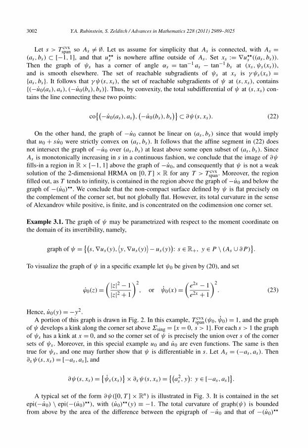


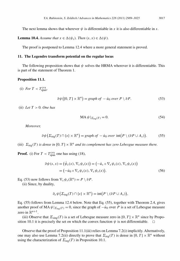

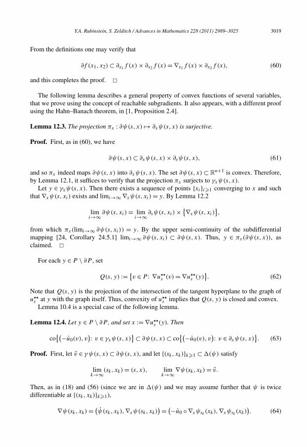


![Interior gradient estimates for solutions to the ... · The linearized Monge–Ampère equation was studied by Caffarelli and Gutiérrez in [5] where the authors showed that nonnegative](https://static.documents.pub/doc/80x56/5f5b2d06b951d83e9874ce06/interior-gradient-estimates-for-solutions-to-the-the-linearized-mongeaampre.jpg)


