The Cauchy transform - University of Richmondwross/PDF/cauchy.pdf · The Cauchy transform Joseph A....

The Cauchy transform

Joseph A. Cima, Alec Matheson, and William T. Ross

To Prof. Harold S. Shapiro on the occasion of his seventy-fifth birthday.

1. Motivation

In this expository paper, we wish to survey both past and current work on thespace of Cauchy transforms on the unit circle. By this we mean the collection K ofanalytic functions on the open unit disk D = z ∈ C : |z| < 1 that take the form

(1.1) (Kµ)(z) :=∫

dµ(ζ)1− ζz

,

where µ is a finite, complex, Borel measure on the unit circle T = ∂D. Our motiva-tion for writing this paper stems not only from the inherent beauty of the subject,but from its connections with various areas of measure theory, functional analy-sis, operator theory, and mathematical physics. We will provide a survey of someclassical results, some of them dating back to the beginnings of complex analy-sis, in order to prepare a reader who wishes to study some recent and importantwork on perturbation theory of unitary and compact operators. We also gather upthese results, which are often scattered throughout the mathematical literature, toprovide a solid bibliography, both for historical preservation and for further study.

Why is the Cauchy transform important? Besides its obvious use, via Cauchy’sformula, in providing an integral representation of analytic functions, the Cauchytransform (with dµ = dm - normalized Lebesgue measure on the unit circle) is theRiesz projection operator f → f+ on L2 := L2(T,m), where the Fourier expansionsof f and f+ are given by

f ∼∞∑

n=−∞anζ

n and f+ ∼∞∑

n=0

anζn.

Questions such as which classes of functions on the circle are preserved (continu-ously) by the Riesz projection were studied by Riesz, Kolmogorov, Privalov, Stein,and Zygmund. For example, the Lp(1 < p <∞) and Lipschitz classes are preservedunder the Riesz projection operator while L1, L∞, and the space of continuousfunctions are not. With the Riesz projection operator, we can define the Toeplitzoperators f → Tφ(f) := (φf)+, where φ ∈ L∞. Questions about continuity, com-pactness, etc., depend not only on properties of the symbol φ but on how the

2 Joseph A. Cima, Alec Matheson, and William T. Ross

Cauchy transform acts on the underlying space of functions f . The Cauchy trans-form is also related to the classical conjugation operator Qµ = 2=(Kµ), at leastfor real measures µ, and similar preservation and continuity questions arise.

Though this classical material is certainly both elegant and important, ourreal inspiration for wanting to write this survey is the relatively recent work be-ginning with a seminal paper of Clark [18] which relates the Cauchy transformto perturbation theory. Due to recent advances of Aleksandrov [4] and Poltoratski[65, 66, 67], this remains an active area of research rife with many interesting prob-lems connecting Cauchy transforms to a variety of ideas in classical and modernanalysis.

Let us take a few moments to describe the basics of Clark’s results. Accordingto Beurling’s theorem [25, p. 114], the subspaces of the classical Hardy space H2

invariant under the unilateral shift Sf = zf have the form ϑH2, where ϑ is aninner function. Consequently, the backward shift operator

S∗f =f − f(0)

z

has invariant subspaces (ϑH2)⊥. A description of (ϑH2)⊥, involving the concept ofa ’pseudocontinuation’, can be found in [16, 24, 75]. Clark studied the compression

Sϑ = PϑS|(ϑH2)⊥

of the shift S to the subspace (ϑH2)⊥, where Pϑ is the orthogonal projection of H2

onto (ϑH2)⊥ (see [60, p. 18]), and determined that all possible rank-one unitaryperturbations of Sϑ (in the case where ϑ(0) = 0) are given by

Uαf := Sϑf +⟨f,ϑ

z

⟩α, α ∈ T.

Furthermore, Uα is unitarily equivalent to the operator ‘multiplication by z’, g →zg, on the space L2(σα), where σα is a certain singular measure on T naturallyassociated with the inner function ϑ. This equivalence is realized by the unitaryoperator

Fα : (ϑH2)⊥ → L2(σα),

which maps the reproducing kernel

kϑλ(z) =

1− ϑ(λ)ϑ(z)1− λz

for (ϑH2)⊥ to the function

ζ → 1− ϑ(λ)α1− λζ

in L2(σα) and extends by linearity and continuity. This measure σα arises asfollows: For each α ∈ T the analytic function

(1.2)α+ ϑ(z)α− ϑ(z)

The Cauchy transform 3

on the unit disk has positive real part, which, by Herglotz’s theorem [25, p. 3],takes the form

<( α+ ϑ(z)α− ϑ(z)

)=

∫T

1− |z|2

|ζ − z|2dσα(ζ),

where the right-hand side of the above equation is the Poisson integral (Pσα)(z)of a positive measure σα. Without too much difficulty, one can show that themeasure σα is carried by the set ζ ∈ T : ϑ(ζ) = α and hence singular withrespect to Lebesgue measure on the circle. Moreover, the measures (σα)α∈T arepairwise singular.

This idea extends via eq.(1.2) beyond inner functions ϑ to any φ in the unitball of H∞ to create a family of positive measures (µα)α∈T associated with φ. Onthe other hand, for a given positive measure µ, the Poisson integral Pµ of µ is apositive harmonic function on the disk and so

(1.3) Pµ = <( 1 + φ

1− φ

)for some φ ∈ ball(H∞). That is to say, every positive measure µ is the Clarkmeasure µ1 for some φ in the unit ball of H∞. It is worth mentioning that φis an inner function if and only if the boundary function for (1 + φ)/(1 − φ) ispurely imaginary. Using eq.(1.3) as well as Fatou’s theorem (which says that theboundary function for Pµ1 is dµ1/dm almost everywhere [25, p. 4]), we concludethat φ is inner if and only if µ1 ⊥ m.

The family (µα)α∈T of Clark measures for some function φ ∈ ball(H∞) alsoprovide a disintegration of normalized Lebesgue measure m on the circle. A beau-tiful theorem of Aleksandrov [4] says that∫

Tµα dm(α) = m,

where the integral is interpreted in the weak-∗ sense, that is,∫T

[ ∫Tf(ζ) dµα(ζ)

]dm(α) =

∫Tf(ζ) dm(ζ)

for all continuous functions f on T. Moreover, if Σ = ζ ∈ T : |φ(ζ)| = 1 ,∫Tµs

α dm(α) = χΣ ·m and∫

Tµac

α dm(α) = (1− χΣ) ·m,

where µsα is the singular part and µac

α is the absolutely continuous part of µα (withrespect to Lebesgue measure m), and again, the above equation is interpreted inthe weak-∗ sense.

One can show that the Cauchy transform of σα (a Clark measure for theinner function ϑ)

(Kσα)(z) =∫

11− ζz

dσα(ζ)


is equal to the function1

1− αϑ(z).

Furthermore, one can use this to produce the following formula for F∗α : L2(σα) →

(ϑH2)⊥ in terms of the ‘normalized’ Cauchy transform

F∗αf =

K(f dσα)K(σα)

.

Poltoratski [65] showed that some striking things happen here. The first is that forσα-almost every ζ ∈ T, the non-tangential limit of the above normalized Cauchytransform exists and is equal to f(ζ). On the other hand, for g ∈ (ϑH2)⊥, thenon-tangential limits certainly exist almost everywhere with respect to Lebesguemeasure on the circle (since (ϑH2)⊥ ⊂ H2). But in fact, for σα-almost every ζ, thenon-tangential limit of g exists and is equal to (Fαg)(ζ). Remarkable here is thesignificance of the role Cauchy transforms play not only in the above perturbationproblem involving the rank-one perturbations of the model operator Sϑ but inother perturbation problems as well (see [67] and the references therein).

After a brief historical introduction in §2, we begin in §3 with a descriptionof some of the classical function theoretic properties of Cauchy transforms, viewedas functions on the unit disk. This will include their boundary and mapping prop-erties, as well as their relationships with the classical Hardy spaces Hp. In §4 weexplore the general question: Which analytic functions on the disk can be rep-resented as Cauchy transforms of measures on the circle? Though the answer tothis question is still incomplete, there is a related result of Aleksandrov, extendingwork of Tumarkin, which characterizes the analytic functions on C\T which areCauchy transforms of measures on the circle.

The space of Cauchy transforms can be viewed in a natural way as the dualspace of the disk algebra, or equivalently, as the quotient space M/H1

0 . We willdescribe this duality in §5, including facts about the weak and weak-∗ topologyon this space. In §6 we will describe multiplication and division in the space ofCauchy transforms and examine such questions as: (i) Which bounded analyticfunctions φ on the disk satisfy φK ⊆ K (the multiplier question)? (ii) If ϑ is innerand divides Kµ, that is, Kµ/ϑ ∈ Hp for some p > 0, does Kµ/ϑ belong to K (thedivisor question)? In §7 we explore the classical operators on Hp (forward andbackward shifts, composition operators, and the Cesaro operator) in the settingof the space of Cauchy transforms. Questions relating to continuity and invariantsubspaces will be explored. In §8 we will touch more briefly on such topics asthe distribution of boundary values of Cauchy transforms. This will include theHavin-Vinogradov-Tsereteli theorem, and its recent improvement by Poltoratski,as well as Aleksandrov’s weak-type characterization using the A-integral. We willalso discuss the maximal properties of Cauchy transforms arising in the recentwork of Poltoratski.

Conspicuously missing from this survey are results about the Cauchy trans-form of a measure compactly supported in the plane. Certainly this is an important


object to study and there are many wonderful ideas here. However, broadening thesurvey to include those Cauchy transforms opens up such a vast array of topicsfrom so many other fields of analysis such as potential theory and partial differ-ential equations, that our original theme and motivation for writing this survey -a brief overview of the subject with a solid bibliography for further study - wouldbe lost. We feel that focusing on the Cauchy transform of measures on the circlelinks the classical function theory with more modern applications to perturbationtheory. If one is interested in exploring the Cauchy transform of a measure on theplane we suggest that the books [9, 28, 61] are a good place to start.

2. Some early history

In a series of papers from the mid 1800’s [86], Cauchy developed what is knowntoday as the ‘Cauchy integral formula’: If f is analytic in |z| < 1 + ε for someε > 0, then

f(z) =1

2πi

∫T

f(ζ)ζ − z

dζ, |z| < 1.

After Cauchy, others, such as Sokhotski, Plemelj, and Privalov [58], examinedthe ‘Cauchy integral’

φ(z) =1

2πi

∫T

φ(ζ)ζ − z

dζ,

where the boundary function f(ζ) in Cauchy’s formula is replaced by a ‘suitable’function φ defined only on the unit circle T. Amongst other things, they exploredthe relationship between the density function φ and the limiting values of φ, as|z| → 1, as well as the Cauchy principal-value integral

12πi

P.V.

∫T

φ(ζ)ζ − eiθ

dζ.

In particular, Sokhotski [87] in his 1873 thesis (see also [54, Vol. I, p. 316]) provedthe following.

Theorem 2.1 (Sokhotski, 1873). Suppose φ is continuous on T and, for a particularζ0 ∈ T, satisfies the condition

|φ(ζ)− φ(ζ0)| 6 C|ζ − ζ0|α, ζ ∈ T

for some positive constants C and α. Then the limits

φ−(ζ0) := limr→1−

φ(rζ0) and φ+(ζ0) := limr→1−

φ(ζ0/r)

exist and moreover, φ−(ζ0)− φ+(ζ0) = φ(ζ0). Furthermore, the Cauchy principal-value integral

P.V.

∫T

φ(ζ)ζ − ζ0

dζ := limε→0

∫|ζ−ζ0|>ε

φ(ζ)ζ − ζ0

dζ


exists and

φ+(ζ0) + φ−(ζ0) =1πiP.V.

∫T

φ(ζ)ζ − ζ0

dζ.

Though Sokhotski first proved these results in 1873, the above formulas areoften called the ‘Plemelj formulas’ due to reformulations and refinements of themby J. Plemelj [64] in 1908.

I. I. Privalov, in a series of papers and books1, beginning with his 1919 Saratovdoctoral dissertation [70], began to examine the Plemelj formulas for integrals ofCauchy-Stieltjes type

F (z) :=1

2πi

∫[0,2π]

11− e−iθz

dF (θ),

where F is a function of bounded variation on [0, 2π]. Privalov, knowing the re-cently discovered integration theory of Lebesgue and following the lead of histeacher Golubev [30], developed the Sokhotski-Plemelj formulas for these Cauchy-Stieltjes integrals.

Theorem 2.2 (Privalov, 1919). Suppose F is a function of bounded variation on[0, 2π]. Then for almost every t, F−(eit), the non-tangential limit of F (z) as z →eit (|z| < 1) and F+(eit), the non-tangential limit at z → eit (|z| > 1), exist andmoreover, F−(eit)− F+(eit) = F ′(t). Furthermore, for almost every t, the Cauchyprincipal-value integral

P.V.

∫[0,2π]

11− e−iθeit

dF (θ) := limε→0

∫|t−θ|>ε

11− e−iθeit

dF (θ)

exists and

F+(eit) + F−(eit) =1πiP.V.

∫[0,2π]

11− e−iθeit

dF (θ).

A well-known theorem from Fatou’s 1906 thesis [26] (see also [25, p. 39])states that F (reit) − F (eit/r) → F ′(t) as r → 1−, whenever F ′(t) exists (whichis almost everywhere). Privalov’s contribution was to prove the existence of theprincipal-value integral as well as to generalize to the case when the unit circle isreplaced with a general rectifiable curve (see [31, 58] for more).

A question explored for some time, and for which there is still no completelysatisfactory answer is: Which analytic functions f on D can be represented as aCauchy-Stieltjes integral? Perhaps a first step in answering this question would beto determine which functions can be represented as the Cauchy integral of theirboundary values. The following theorem of the brothers Riesz [72] (see also [25, p.41]) gives the answer 2.

1There is Privalov’s famous book [71] as well as a nice survey of his work in [53].2A nice survey of these results (and others) can be found in [31, Ch. IX].


Theorem 2.3 (F. and M. Riesz). Let f be analytic on D. Then f has an almosteverywhere defined, integrable - with respect to Lebesgue measure on T - non-tangential limit function f∗ and

f(z) =1

2πi

∫T

f∗(ζ)ζ − z

dζ, z ∈ D

if and only if f belongs to H1.

Though the question as to which analytic functions on D can be representedas Cauchy integrals of their boundary functions has been answered, there is nocomplete description of these functions, though there are some nice partial results(see Theorem 4.9 below).

To give the reader some historical perspective, we stated these classical the-orems of Sokhotski, Plemelj, Riesz, and Privalov, in terms of Cauchy-Stieltjesintegrals of functions of bounded variation. However, for the rest of this survey, wewill use the more modern, but equivalent, notation of Cauchy integrals of finite,complex, Borel measures on the circle as in eq.(1.1). This is done by equating afunction of bounded variation with a corresponding measure and vice-versa (see[39, p. 331] for further details).

3. Some basics about the Cauchy transform

Before moving on, let us set some notation. Throughout this survey, C will denotethe complex numbers, C := C ∪ ∞ the Riemann sphere, D := |z| < 1 theopen unit disk, D− := |z| 6 1 its closure, T := ∂D = |z| = 1 its boundary,and De := C \ D− will denote the (open) extended exterior disk. M := M(T) willdenote the complex, finite, Borel measures on T, M+ the positive measures in M ,Ma := µ ∈ M : µ m (dm = |dζ|/2π is normalized Lebesgue measure onthe circle), and Ms := µ ∈ M : µ ⊥ m. The norm on M , the total variationnorm, will be denoted by ‖µ‖. The Lebesgue decomposition theorem says thatM = Ma⊕Ms and that if µ = µa+µs (µa ∈Ma, µs ∈Ms), then ‖µ‖ = ‖µa‖+‖µs‖.

For 0 < p 6 ∞ we will let Lp := Lp(m) denote the usual Lebesgue spaces,Hp the standard Hardy spaces, and ‖ · ‖p the norm on these spaces. When p = ∞,H∞ will denote the bounded analytic functions on D. Recall that every function inHp has finite non-tangential limits almost everywhere and this boundary functionbelongs to Lp. In fact, the Lp norm of this boundary function is the Hp norm.We will use N to denote the Nevanlinna class of the disk and N+ to denote theSmirnov class. We refer the reader to some standard texts about the Hardy spaces[25, 29, 40, 51, 77].

The following theorem of F. and M. Riesz [25, p. 41] plays an important rolein the theory of Cauchy transforms and will be mentioned many times in thissurvey.


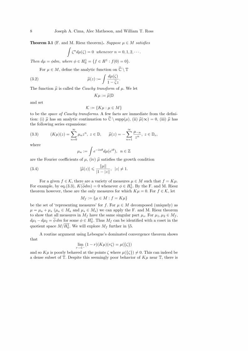
Theorem 3.1 (F. and M. Riesz theorem). Suppose µ ∈M satisfies∫ζndµ(ζ) = 0 whenever n = 0, 1, 2, · · · .

Then dµ = φdm, where φ ∈ H10 = f ∈ H1 : f(0) = 0.

For µ ∈M , define the analytic function on C \ T

(3.2) µ(z) :=∫

dµ(ζ)1− ζz

.

The function µ is called the Cauchy transform of µ. We let

Kµ := µ|Dand set

K := Kµ : µ ∈Mto be the space of Cauchy transforms. A few facts are immediate from the defini-tion: (i) µ has an analytic continuation to C \ supp(µ), (ii) µ(∞) = 0, (iii) µ hasthe following series expansions:

(3.3) (Kµ)(z) =∞∑

n=0

µnzn, z ∈ D, µ(z) = −

∞∑n=1

µ−n

zn, z ∈ De,

where

µn :=∫e−inθdµ(eiθ), n ∈ Z

are the Fourier coefficients of µ, (iv) µ satisfies the growth condition

(3.4) |µ(z)| 6 ‖µ‖|1− |z||

, |z| 6= 1.

For a given f ∈ K, there are a variety of measures µ ∈M such that f = Kµ.For example, by eq.(3.3), K(φdm) = 0 whenever φ ∈ H1

0 . By the F. and M. Riesztheorem however, these are the only measures for which Kµ = 0. For f ∈ K, let

Mf := µ ∈M : f = Kµbe the set of ‘representing measures’ for f . For µ ∈ M decomposed (uniquely) asµ = µa + µs (µa ∈ Ma and µs ∈ Ms) we can apply the F. and M. Riesz theoremto show that all measures in Mf have the same singular part µs. For µ1, µ2 ∈Mf ,dµ1− dµ2 = φdm for some φ ∈ H1

0 . Thus Mf can be identified with a coset in thequotient space M/H1

0 . We will explore Mf further in §5.

A routine argument using Lebesgue’s dominated convergence theorem showsthat

limr→1−

(1− r)(Kµ)(rζ) = µ(ζ)

and so Kµ is poorly behaved at the points ζ where µ(ζ) 6= 0. This can indeed bea dense subset of T. Despite this seemingly poor behavior of Kµ near T, there is


some regularity in the boundary behavior of a Cauchy transform. For 0 < p 6 ∞,let Hp(C \ T) denote the class of analytic functions f on C \ T for which

‖f‖p

Hp(C\T):= sup

r 6=1

∫T|f(rζ)|pdm(ζ) <∞.

A well-known theorem of Smirnov [85] (see also [25, p. 39]) is the following.

Theorem 3.5 (Smirnov). If µ ∈M , then

µ ∈⋂

0<p<1

Hp(C \ T)

and moreover, ‖µ‖Hp(C\T) 6 cp‖µ‖, where cp = O((1− p)−1).

The above theorem says that for fixed 0 < p < 1, the operator µ → Kµ isa continuous linear operator from M to Hp. What is the norm of this operator?Equivalently, what is the best constant Ap in the estimate ‖Kµ‖p 6 Ap‖µ‖? Wedo not know the answer to this. However, we can say that

sup‖Kµ‖p : µ ∈M+, ‖µ‖ = 1 = ‖ 11− z

‖p.

To see this note that Kµ is subordinate to φ(z) = (1−z)−1. Now use Littlewood’ssubordination theorem [25, p. 10]. For any complex measure µ = (µ1 − µ2) +i(µ3−µ4), µj > 0, one can use a slight variation of the above argument four timesto prove Smirnov’s theorem: ‖Kµ‖p 6 Ap‖µ‖. However, the best constant Ap isunknown for general complex measures.

The containmentK

⋂0<p<1

Hp

is strict since f(z) = (1 − z)−1 log(1 − z) ∈ Hp for all 0 1) can be written as the Cauchyintegral of its boundary function. Thus⋃

p>1

Hp K ⋂

0<p<1

Hp.

The first containment above is strict since (1 − z)−1 = Kδ1 but does not belongto H1. For 0 < p < 1, the boundary functions for Hp functions certainly belongto Lp. However, they may not be integrable on the circle and so their Cauchyintegral does not always make sense. There is a remedy for this in the theory of‘A-integrals’ that will be described in §4, which says that some, but not all, Cauchytransforms can be written as the Cauchy A-integral of their boundary functions.

Smirnov’s theorem has been refined in a variety of ways. The first refinementdue to M. Riesz [73] (see also [25, p. 54]) deals with the case when the measure µ


takes the form dµ = fdm for f ∈ Lp (1 < p < ∞). Since the notation K(fdm)can be a bit cumbersome, we use f+ to denote K(fdm) for f ∈ L1.

Theorem 3.6 (M. Riesz). If 1 < p <∞ then f+ ∈ Hp whenever f ∈ Lp. Moreover,the map f → f+ from Lp to Hp is continuous and onto.

For f ∈ Lp (1 < p <∞) with Fourier series

f ∼∞∑

n=−∞fnζ

n, fn :=∫ 2π

0

e−inθf(eiθ)dθ

2π,

it is not too difficult to see that the Lp boundary function for f+ has Fourier series

f+ ∼∞∑

n=0

fnζn.

Thus we can think of the Cauchy transform as projection operator P : Lp → Hp,Pf = f+. Hollenbeck and Verbitsky [41] compute the norm of the Riesz projectionas

sup‖f+‖p : ‖f‖Lp= 1 =

1sin(π/p)

, 1 < p <∞.

The endpoint cases p = 1 and p = ∞ are more complicated. For example [25,pp. 63 - 64], the f ∈ L1 whose Fourier series is

∞∑n=2

cosnθlog n

has Cauchy transform equal to

f+ =∞∑

n=2

zn

log n

which does not belong to H1 [25, p. 48]3. It is worth remarking here that notonly does the Riesz projection f → f+ fail to be continuous from L1 onto H1,but there is no other continuous projection of L1 onto H1 [59]. If the function isslightly better than L1, there is the following theorem of Zygmund [100] (see also[25, p. 58]): If |f | log+ |f | ∈ L1, then f+ ∈ H1.

Despite these pathologies with p = 1, there is a well-known, and often re-visited, theorem about the Cauchy transforms of L1 functions due to Kolmogorov[50] (see also [51, p. 92]).

Theorem 3.7 (Kolmogorov).For f ∈ L1,

m(|f+| > λ) 6 A‖f‖1λ

, λ > 0.

3If f =∑

n anzn ∈ H1, then∑

n |an|/(n + 1) 6 π‖f‖1.


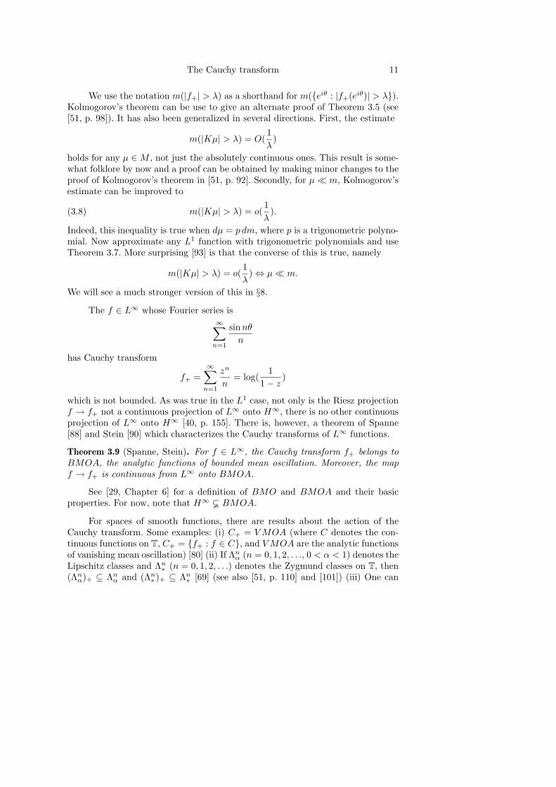
We use the notation m(|f+| > λ) as a shorthand for m(eiθ : |f+(eiθ)| > λ).Kolmogorov’s theorem can be use to give an alternate proof of Theorem 3.5 (see[51, p. 98]). It has also been generalized in several directions. First, the estimate

m(|Kµ| > λ) = O(1λ

)

holds for any µ ∈M , not just the absolutely continuous ones. This result is some-what folklore by now and a proof can be obtained by making minor changes to theproof of Kolmogorov’s theorem in [51, p. 92]. Secondly, for µ m, Kolmogorov’sestimate can be improved to

(3.8) m(|Kµ| > λ) = o(1λ

).

Indeed, this inequality is true when dµ = p dm, where p is a trigonometric polyno-mial. Now approximate any L1 function with trigonometric polynomials and useTheorem 3.7. More surprising [93] is that the converse of this is true, namely

m(|Kµ| > λ) = o(1λ

) ⇔ µ m.

We will see a much stronger version of this in §8.

The f ∈ L∞ whose Fourier series is∞∑

n=1

sinnθn

has Cauchy transform

f+ =∞∑

n=1

zn

n= log(

11− z

)

which is not bounded. As was true in the L1 case, not only is the Riesz projectionf → f+ not a continuous projection of L∞ onto H∞, there is no other continuousprojection of L∞ onto H∞ [40, p. 155]. There is, however, a theorem of Spanne[88] and Stein [90] which characterizes the Cauchy transforms of L∞ functions.

Theorem 3.9 (Spanne, Stein). For f ∈ L∞, the Cauchy transform f+ belongs toBMOA, the analytic functions of bounded mean oscillation. Moreover, the mapf → f+ is continuous from L∞ onto BMOA.

See [29, Chapter 6] for a definition of BMO and BMOA and their basicproperties. For now, note that H∞ BMOA.

For spaces of smooth functions, there are results about the action of theCauchy transform. Some examples: (i) C+ = VMOA (where C denotes the con-tinuous functions on T, C+ = f+ : f ∈ C, and VMOA are the analytic functionsof vanishing mean oscillation) [80] (ii) If Λn

α (n = 0, 1, 2, . . ., 0 < α < 1) denotes theLipschitz classes and Λn

∗ (n = 0, 1, 2, . . .) denotes the Zygmund classes on T, then(Λn

α)+ ⊆ Λnα and (Λn

∗ )+ ⊆ Λn∗ [69] (see also [51, p. 110] and [101]) (iii) One can


check just by looking at Fourier and power series coefficients that if f ∈ C∞(T),then every derivative of f+ has a continuous extension to the closed disk D−.

What about Cauchy transforms of functions from weighted Lp spaces? Thequestion here is the following: Given 1 < p < ∞, what are the conditions on ameasure µ ∈M+ (the non-negative measures in M) such that∫

|g+|pdµ 6 C

∫|g|pdµ

for all trigonometric polynomials g? Though there has been earlier work on thisproblem [32, 38] (for example dµ must take the form wdm), the definitive resulthere is a celebrated theorem of Hunt, Muckenhoupt, and Wheeden [45] (a precisecondition on the weight w called the ‘Ap condition’).

In looking at the references for the above results, one notices that they alldeal with ‘conjugate functions’ (fonctions conjuguees). The relationship betweenthis conjugation operator and the Cauchy transform is as follows. A computationreveals that

11− ζz

=12

[1 + Pz(ζ) + iQz(ζ)

],

where

(3.10) Pz(ζ) =1− |z|2

|ζ − z|2Qz(ζ) =

2=(ζz)|ζ − z|2

, ζ ∈ T, z ∈ D,

are the Poisson and conjugate Poisson kernels. For f ∈ L1,

f+(z) =12

[ ∫Tf(ζ)dm(ζ) +

∫TPz(ζ)f(ζ)dm(ζ) + i

∫TQz(ζ)f(ζ)dm(ζ)

].

By Fatou’s theorem [25, p. 5],

lim]z→eiθ

∫TPz(ζ)f(ζ)dm(ζ) = f(eiθ) a.e.

and [101, Vol. I, p. 131] the following limit

f(eiθ) := lim]z→eiθ

∫TQz(ζ)f(ζ)dm(ζ)

exists for almost all eiθ. Here ] denotes the non-tangential limit. Moreover,

f(eiθ) = limε→0+

12π

∫|θ−t|>ε

cot( θ − t

2)f(eit) dt a.e.

One can also define, for µ ∈M ,

(Qµ)(z) =∫Qz(ζ)dµ(ζ)


and note that the above function has non-tangential limits almost everywheredenoted by µ(eiθ). The operator f → f (or µ → µ) is called the conjugationoperator. Thus, for example,

f+(eiθ) =12

[ ∫Tf(ζ)dm(ζ) + f(eiθ) + if(eiθ)

]a.e.

Thus questions about the continuity of the operator f → f+ (on spaces of functionson T) are equivalent to questions about the continuity of the conjugation operatorf → f . The norm of the operator f → f+ is known when 1 1 and anoperator from L1 to Lp for 0 2; (cos(pπ/2))−1/p‖f‖1 6 ‖f‖p 621/p−1(cos(pπ/2))−1/p‖f‖1 for 0 < p < 1.

A variant of Kolmogorov’s theorem (Theorem 3.7) says that for fixed 0 <p < 1 and µ ∈M , µ belongs to Lp and

‖µ‖Lp 6 cp‖µ‖.

B. Davis [19, 20, 21] computes the best constant cp, at least for real measures MRas

sup‖µ‖Lp : µ ∈MR, ‖µ‖ = 1 = ‖ν‖Lp ,

where ν is a measure given by ν(1) = 1/2, ν(−1) = −1/2 and |ν|(T\−1, 1) =0.

Kolmogorov’s theorem says that

m(|Kµ| > λ) 6 C‖µ‖λ, µ ∈M.

The best constant C is unknown. However, there is information about the bestconstant in the related inequality

m(|µ| > λ) 6 C‖µ‖λ.

When µ dm, the best constant C is Θ−1, where Θ = (1− 3−2 +5−2−· · · )/(1+3−2 + 5−2 + · · · ). For µ ∈M+, the best constant C is one.

Here is a good place to mention that the conjugation operator Q is closelyrelated to the Hilbert transform

(Hf)(x) := P.V.1π

∫ ∞

−∞

f(t)x− t

dt,

defined almost everywhere for f ∈ L1(R, dx). Results for the conjugation operatorfrequently have direct analogs for the Hilbert transform in that they are bothsingular integral operators [29, 91].


4. Which analytic functions are Cauchy transforms?

For an analytic f on D, when is f = Kµ? Gathering up the observations fromprevious sections of this survey, there are the following necessary conditions.

Proposition 4.1. Suppose f = Kµ for some µ ∈M . Then1. f satisfies the growth condition |f(z)| 6 Cµ(1− |z|)−1.2. f has finite non-tangential limits m-almost everywhere on T and

m(|f | > λ) 6 Cf/λ, λ > 0.

3. f ∈ Hp for all 0 0 anz

n, then (an)n>1 is a bounded sequence of complex num-bers.

Known necessary and sufficient conditions for an analytic function on the diskto be a Cauchy transform are difficult to apply and in a way, the very question isunfair. For example, suppose that f is analytic on D with power series

f(z) = a0 + a1z + a2z2 + · · ·

and we want to know if f = Kµ on D for some µ ∈ M . Since, from eq.(3.3), Kµcan be written as

(Kµ)(z) = µ0 + µ1z + µ2z2 + · · · ,

we would be trying to determine (comparing an with µn) the measure µ from only‘half’ its Fourier coefficients (the non-negative ones).

If one can settle for a functional analysis condition, there is characterizationof K [33], albeit difficult to apply. The proof follows directly by a duality argument(see §5 below).

Theorem 4.2 (Havin). Suppose f =∑∞

k=0 akzk is analytic on D. Then the following

statements are equivalent.1. There is some constant C > 0, depending only on f , such that∣∣ p∑

k=0

λkak

∣∣6 Cmax∣∣ p∑

k=0

λk

zk+1

∣∣: z ∈ T for any complex numbers λ0, . . . , λp.

2. f = Kµ for some µ ∈M .

Instead of asking whether or not an analytic function defined only on D isa Cauchy transform, suppose we were to ask if an analytic function f on C\T isa Cauchy transform µ on C\T (recall the definition of µ from eq.(3.2)). This is amore tractable question since we would be comparing the Laurent series of thesetwo functions which would involve knowing all of the Fourier series coefficients ofµ and not just the non-negative ones as before (see eq.(3.3)). An early result whichanswers this question is one of Tumarkin [95] (see [55] for a generalization).


Theorem 4.3 (Tumarkin). Let f be analytic on C \ T with f(∞) = 0 and setf1 = f |D and f2 = f |De. Then f = µ for some µ ∈M if and only if

(4.4) sup0<r<1

∫T|f1(rζ)− f2(ζ/r)|dm(ζ) <∞.

The Havin and Tumarkin results are easily seen to be equivalent using thetechnique of dual extremal problems as pioneered by S. Ja. Khavinson [36, 37] andW. Rogosinski and H. S. Shapiro [74].

There is a refinement of Tumarkin’s due to Aleksandrov [2, Thm. 5.3] whicheven identifies the type of representing measure µ for f . From the previous section,a Cauchy transform f = µ on C\T satisfies the four conditions

(4.5) f(∞) = 0,

(4.6) f ∈⋂

0<p<1

Hp(C \ T),

(4.7) ‖f‖Hp(C\T) = O(1

1− p),

(4.8) Jf ∈ L1, (Jf)(ζ) := limr→1−

[f(rζ)− f(ζ/r)

].

Theorem 4.9 (Aleksandrov). Let f be an analytic function on C \ T satisfyingthe conditions in eq.(4.5) through eq.(4.8) above. Then f = µ for some µ ∈ M .Moreover, if the conditions in eq.(4.5) and eq.(4.6) are satisfied, then

1. f = µ for some µ dm if and only if

limp→1−

‖f‖Hp(C\T)(1− p) = 0

and Jf ∈ L1.2. f = µ for some µ ⊥ dm if and only if

limp→1−

‖f‖Hp(C\T)(1− p) <∞

and Jf = 0 m-almost everywhere.

There is even a further refinement. Let X be a class of analytic functions onD and E be a closed subset of T. Let F(X,E) denote the functions f ∈ X suchthat f = Kµ, where µ ∈M and has support in E. Under what conditions on E isF(X,E) 6= (0)? When 0 1, Havin proves that F(Hp, E) 6= (0) if and onlym(E) > 0 [34]. Though the analysis is more complicated, Hruscev [42] answersthis question for the disk algebra and various other spaces of functions that aresmooth up to the boundary.


We close this section by mentioning the following generalization of the Cauchyintegral formula involving the theory of A-integrals as studied by Denjoy, Titch-marsh, Kolmogorov, Ul’yanov, and Aleksandrov. A measurable function g : T→ Cis A-integrable if

(4.10) m(|g| > t) = o(1/t)

and

(A)∫g(ζ)dm(ζ) := lim

t→∞

∫|g|<t

g(ζ)dm(ζ)

exists. For µ ∈ M with µ m, f = Kµ has non-tangential boundary values m-almost everywhere and, by eq.(3.8), f satisfies the condition in eq.(4.10). However,this Cauchy transform may not belong to H1 and so cannot be recovered from itsboundary function via the Cauchy integral formula. A theorem of Ul’yanov [96] isthe substitute ‘Cauchy A-integral formula’.

Theorem 4.11 (Ul’yanov). For µ ∈ M with µ m, the function f = Kµ isA-integrable and

(4.12) f(z) =1

2πi(A)

∫T

f(ζ)ζ − z

dζ, z ∈ D.

A theorem of Aleksandrov [1] says that if f ∈ N+ (the Smirnov class) satisfiesm(|f | > t) = o(1/t) as t → ∞ then eq.(4.12) holds. The condition in eq.(4.10)cannot be weakened since the function i(1 + z)/(1 − z) cannot be written as theCauchy A-integral of its boundary values. More about this can be found in thereferences in [79]. There is even a version of the conjugation operator using A-integrals in [8] and moreover, this book also contains a nice historical treatmentof A-integrals.

5. Topology on the space of Cauchy transforms

In this section we consider the space K of Cauchy transforms as a Banach space.We will show how it arises naturally as the dual space to the disk algebra A andindicate its relationship to the space of measures M .

Let C = C(T) denote the Banach space of complex-valued continuous func-tions on the unit circle endowed with the supremum norm ‖f‖∞. Every µ ∈ Mdetermines a bounded linear functional `µ on C by

`µ(f) :=∫

Tf dµ

with norm equal to the total variation norm ‖µ‖ of µ. Conversely, the Riesz repre-sentation theorem [77] guarantees that every bounded linear functional on C hassuch a representation, and in fact the map µ → `µ is an isometric isomorphismfrom M onto C∗ (the dual space of C). Thus, by tradition, we identify C∗ withM .


The disk algebra A is the closure of the analytic polynomials in C or equiv-alently, the space of functions analytic on D that have continuous extensions toD−. Its annihilator A⊥ is a closed subspace of C∗ 'M which we identify with theset of measures µ ∈M for which∫

gdµ = 0 for all g ∈ A.

By the F. and M. Riesz theorem (Theorem 3.1), such annihilating measures µtake the form dµ = fdm, where f ∈ H1

0 and so we identify A⊥ and H10 . We

can identify C∗/A⊥ with A∗ via the mapping `µ + A⊥ → `µ|A and furthermore,endowing C∗/A⊥ with the usual quotient space norm

‖`µ +A⊥‖ = dist(`µ, A⊥),

the above mapping is an isometric isomorphism [78, pp. 96 - 97]. Putting this alltogether, we have

A∗ 'M/H10 ,

where, as before, ' denotes an isometric isomorphism.Since Kµ = 0 if and only if µ ∈ A⊥ ' H1

0 , the map µ + H10 → Kµ from

M/H10 to K is bijective. From here it makes sense to endow K with the norm of

M/H10 , that is

‖Kµ‖ := dist(µ,H10 ) = inf‖dµ+ fdm‖ : f ∈ H1

0.

Hence K 'M/H10 .

Finally, recall that for f ∈ K we let Mf = µ ∈ M : f = Kµ be the setof representing measures for f . Since Kµ = Kν if and only if dµ − dν = fdm(f ∈ H1

0 ), it follows that

‖f‖ = inf‖ν‖ : ν ∈Mf.

Gathering up these facts, we have the following summary result.

Theorem 5.1. The norm dual of A can be identified in an isometric and isomorphicway with K via the sesquilinear pairing

(5.2) 〈f,Kµ〉 =∫

Tf dµ,

or equivalently, by a power series computation,

(5.3) 〈f,Kµ〉 = limr→1−

∞∑n=0

fnµnrn,

where (fn)n>0 are the Taylor coefficients of f and (µn)n>0 are the Fourier coeffi-cients of µ.


From the Lebesgue decomposition theorem, the space of measures M admitsa direct sum decomposition

M = L1 ⊕Ms.

where L1 is identified with the absolutely continuous measuresMa. SinceH10 ⊂ L1,

A∗ satisfiesA∗ ' L1/H1

0 ⊕Ms.

Similarly, the space of Cauchy transforms can be decomposed as

K = Ka ⊕Ks,

where Ka = Kµ : µ m and Ks = Kµ : µ ⊥ dm. Furthermore, if µ = µa+µs

(µa m and µs ⊥ m), then

‖Kµ‖ = ‖Kµa‖+ ‖Kµs‖.We point out a few more items of interest. First,

µ ⊥ dm⇒ ‖Kµ‖ = ‖µ‖.

Secondly, Ka ' L1/H10 and is the norm closure of the analytic polynomials in K.

Thirdly, Ks 'Ms and as such is non-separable since Ms is non-separable. Fourth,since, for f ∈ K,

‖f‖ = inf‖ν‖ : ν ∈Mf,there is a sequence of measures (νn)n>1 in Mf such that ‖νn‖ 6 ‖f‖ + 1/n foreach n. If ν is a weak-∗ limit point of (νn)n>1 in M , it follows that ν ∈ Mf and‖Kµ‖ = ‖ν‖. It is known that the measure ν is unique [35, 46]. We denote thisunique representing measure ν by νf . Since all measures in Mf have the samesingular part, a similar theorem holds for Ka. Indeed, if f ∈ Ka, then there is aunique h ∈ L1 such that h dm ∈Mf and ‖f‖ = ‖h‖1.

There is another topology on K namely the weak-∗ topology it inherits frombeing the norm dual of A. The Banach-Alaoglu theorem says that the closed unitball of K is compact. In this case, the weak-∗ topology on bounded sets can becharacterized by its action on sequences. To be specific, we say that a sequence(fn)n>1 ⊂ K converges weak-∗ to zero if 〈g, fn〉 → 0 for every g ∈ A. From thepointwise estimate

(5.4) |f(z)| 6 11− |z|

‖f‖ for all z ∈ D, f ∈ K 4

one can prove that a sequence (fn)n>1 in K converges to f weak-∗ if and only if(fn)n>1 is uniformly bounded in the norm of K and fn(z) → f(z) for each z ∈ D[13, Prop. 2]. Although K is not separable in the norm topology, it is separable inthe weak-∗ topology. This follows from the same fact about M 5 and the weak-∗continuity of the canonical quotient map π : M →M/H1

0 ' K.

4‖f‖ is the norm in K. We know from eq.(3.4) that |f(z)| 6 ‖µ‖(1 − |z|)−1, where µ ∈ Mf .

When µ = µf , then ‖µ‖ = ‖f‖.5In M , the linear span of the unit point masses δζ : ζ = eiθ, θ ∈ Q form a weak-∗ dense set.


Since K, with the norm topology, is a Banach space, it can be endowedwith a weak topology, though the dual space of K is not a readily identifiablespace of analytic functions. There are two interesting theorems regarding this weaktopology on K. The first deals with weak completeness. A Banach space is weaklycomplete (weak Cauchy nets convergence in the space) if and only if it is reflexive(a consequence of Goldstine’s theorem [23, p. 13]) and so K is not weakly complete.However, K is weakly sequentially complete. In general, a sequence (xn)n>1 in aBanach space X is weak Cauchy if the numerical sequence (`(xn))n>1 convergesfor each ` ∈ X∗. Thus X is weakly sequentially complete if every weak Cauchysequence in X converges weakly to some element of X. Mooney’s Theorem [57]asserts that K is weakly sequentially complete and is a consequence of the followingresult: Let (φn)n>1 be a sequence in L1 such that the limit

limn→∞

∫Tφnf dm := L(f)

exists for every f ∈ H∞. Then there is a function φ ∈ L1 such that

L(f) =∫

Tφf dm for all f ∈ H∞.

A proof of this can be found in [29, pp. 206–209]. How does this implyMooney’s theorem? Since H1

0 is the annihilator of H∞ in L1, it follows thatH∞ can be regarded as the dual space of L1/H1

0 . The above theorem is thenjust the statement that L1/H1

0 is weakly sequentially complete. Now notice thatK ' L1/H1

0 ⊕Ms and so K∗ ' H∞ ⊕M∗s . Suppose (φn)n>1 is a weak Cauchy

sequence in K. Each φn has a unique decomposition as φn = ψn + νn, whereψn ∈ Ka and νn ∈ Ks. Because of the direct sum decomposition of K∗, it is evi-dent that each of the sequences (ψn)n>1 and (νn)n>1 is a weak Cauchy sequence.By the result quoted above, the first sequence converges weakly to some ψ ∈ Ka.On the other hand, a theorem of Kakutani says that Ms is isometrically isomor-phic to L1(Ω,Σ, µ) for some abstract measure space (Ω,Σ, µ) [47]. It follows thatMs is weakly sequentially complete since every such space L1(Ω,Σ, µ) is weaklysequentially complete [23].

The second theorem we will present on the weak topology in K is a deepresult due independently to Delbaen [22] and Kisliakov [49]. For each f ∈ K, recallthat µf is the unique measure such that f = Kµf and ‖f‖ = ‖µf‖.

Theorem 5.5. Let W be a weakly compact set in K, and let W = µf : f ∈ W .Then W is relatively weakly compact.

A thorough discussion of this theorem can be found in [62, Ch. 7] or [99]. Thistheorem derives its significance from the Dunford-Pettis Theorem characterizingweakly compact subsets in M . This characterization says that a set W in M isweakly compact if and only if it is bounded and uniformly absolutely continuous(cf. [23]).


We now talk about a basis for K. A sequence (xn)n>1 in a Banach space Xis a Schauder basis for X if every x ∈ X can be written uniquely as

x =∞∑

n=1

cnxn,

where cn are complex numbers and the = sign means convergence in the norm ofX. A sequence (`n)n>1 ⊂ X∗ is called a weak-∗ Schauder basis if every ` ∈ X∗

can be written uniquely as

` =∞∑

n=1

dn`n,

where dn are complex numbers and = means weak-* convergence.For a Schauder basis (xn)n>1, there is a natural sequence (x∗n)n>1 of contin-

uous linear functionals defined by

x∗n(f) = cn, where f =∞∑

n=1

cnxn

(remember that the expansion of f is unique and so x∗n is well-defined). One canprove the following: If (xn)n>1 is a Schauder basis for X, then (x∗n)n>1 is a weak-*Schauder basis for X∗. If (xn)n>1 is a Schauder basis for X, then (x∗n)n>1 is aSchauder basis for its closed linear span [23, p. 52].

Let us apply the above to X = A and X∗ ' K to identify a weak-* Schauderbasis for K and a Schauder basis for Ka ' L1/H1

0 . The result which drives this isone of Bockarev [10] which produces a Schauder basis (bn)n>1 for the disk algebraA. Moreover, by its actual construction, bnn>1 is an orthonormal set in L2. LetBn := (bn)+. We do this to not confuse bn, the element of the disk algebra A, withBn, the element of K. The result here is the following.

Proposition 5.6. (Bn)n>1 is a weak-∗ Schauder basis for K and a Schauder basisfor Ka.

6. Multipliers of the space of Cauchy transforms

For a linear space of analytic functions X on the unit disk, an important collectionof functions are those φ, analytic on D, for which φf ∈ X whenever f ∈ X. Suchφ are called multipliers of X and we denote this class by M(X). For the Hardyspaces Hp (0 < p 6 ∞) it is routine to check that M(Hp) = H∞. For other classesof functions such as the classical Dirichlet space or the Besov spaces, characterizingthe multipliers is more difficult [56, 89]. For the space of Cauchy transforms, themultipliers are not completely understood but they do have several interestingproperties.

For example, there is a nice relationship between multipliers and Toeplitzoperators. If φ ∈ H∞ and Tφ(f) = P (φf) is the co-analytic Toeplitz operator,then the Riesz theorem (Theorem 3.6) says that P , and hence Tφ, is a bounded


operator onHp for 1 < p <∞. When p = ∞, the Riesz projection P is unbounded.However, this following theorem of Vinogradov [97] determines when Tφ is boundedon H∞.

Proposition 6.1. For φ ∈ H∞, the following are equivalent.1. φ ∈M(K).2. φ ∈M(Ka).3. Tφ : A→ A is bounded.4. Tφ : H∞ → H∞ is bounded.

Moreover, ‖Tφ : A→ A‖ is equal to the multiplier norm, see below, of φ.

If φ is a multiplier of K, the closed graph theorem, says that the multiplicationoperator f → φf on K is continuous. The norm of this operator is denoted by ‖φ‖.The weak-∗ density of the convex hull of δζ : ζ ∈ T in the unit ball of M ,together with the identity (Kδζ)(z) = (1− ζz)−1 yields [98]

‖φ‖ = sup∥∥ φ

1− ζz

∥∥K: ζ ∈ T

.

Since the constant functions belong to K, any multiplier belongs to K. Infact, one can show that any multiplier φ is a bounded function on D and satisfies‖φ‖∞ 6 ‖φ‖. This standard fact is true for the multipliers for just about anyBanach space of analytic functions. Although a usable characterization of themultipliers of K is unknown, there are some sufficient conditions one can quicklycheck to see if a given φ ∈ H∞ is a multiplier of K. See [98] for details.

Theorem 6.2 (Goluzina-Havin-Vinogradov). Let φ be an analytic function on D.Then any one of the following conditions imply that φ is a multiplier of K.

1. φ ∈ H∞ and

sup ∫

T

∣∣ φ(ζ)− φ(ξ)ζ − ξ

∣∣ dm(ξ) : ζ ∈ T<∞.

2. φ extends to be continuous on D− and∫0

ω(t)tdt <∞,

where ω is the modulus of continuity of φ.3. The quantity

∞∑n=0

|φ(n)(0)|n!

log(n+ 2)

is finite.

This next theorem says that the multipliers of K are reasonably regular nearthe boundary of D. Again, see [98] for details.

Theorem 6.3. If φ is a multiplier of K, then


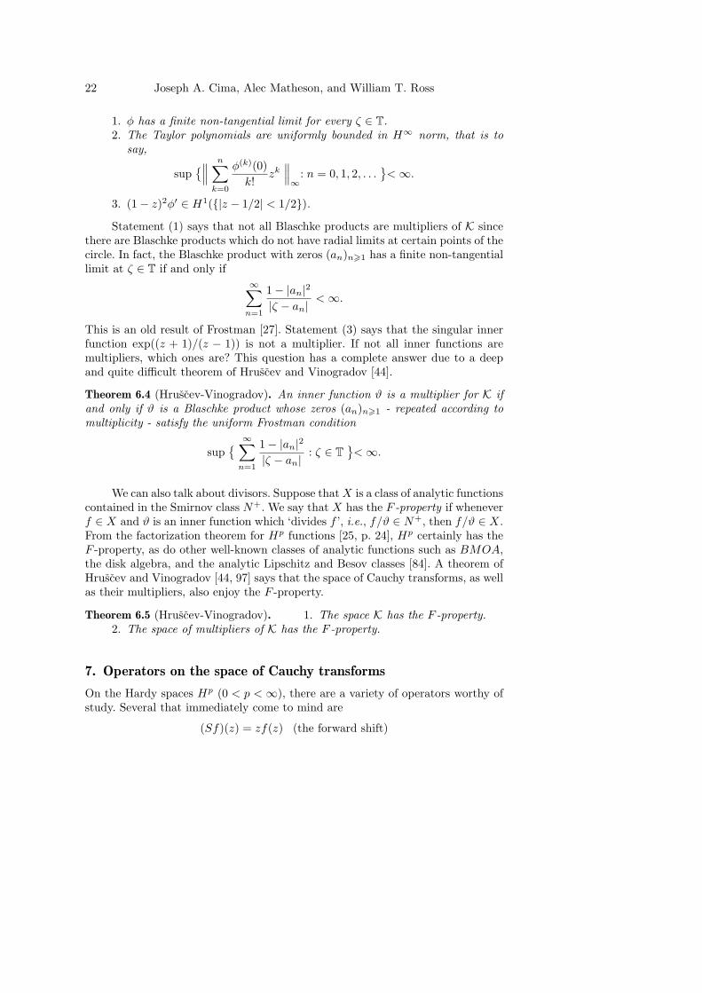
1. φ has a finite non-tangential limit for every ζ ∈ T.2. The Taylor polynomials are uniformly bounded in H∞ norm, that is to

say,

sup∥∥∥ n∑

k=0

φ(k)(0)k!

zk∥∥∥∞

: n = 0, 1, 2, . . .<∞.

3. (1− z)2φ′ ∈ H1(|z − 1/2| < 1/2).

Statement (1) says that not all Blaschke products are multipliers of K sincethere are Blaschke products which do not have radial limits at certain points of thecircle. In fact, the Blaschke product with zeros (an)n>1 has a finite non-tangentiallimit at ζ ∈ T if and only if

∞∑n=1

1− |an|2

|ζ − an|<∞.

This is an old result of Frostman [27]. Statement (3) says that the singular innerfunction exp((z + 1)/(z − 1)) is not a multiplier. If not all inner functions aremultipliers, which ones are? This question has a complete answer due to a deepand quite difficult theorem of Hruscev and Vinogradov [44].

Theorem 6.4 (Hruscev-Vinogradov). An inner function ϑ is a multiplier for K ifand only if ϑ is a Blaschke product whose zeros (an)n>1 - repeated according tomultiplicity - satisfy the uniform Frostman condition

sup ∞∑

n=1

1− |an|2

|ζ − an|: ζ ∈ T

<∞.

We can also talk about divisors. Suppose thatX is a class of analytic functionscontained in the Smirnov class N+. We say that X has the F -property if wheneverf ∈ X and ϑ is an inner function which ‘divides f ’, i.e., f/ϑ ∈ N+, then f/ϑ ∈ X.From the factorization theorem for Hp functions [25, p. 24], Hp certainly has theF -property, as do other well-known classes of analytic functions such as BMOA,the disk algebra, and the analytic Lipschitz and Besov classes [84]. A theorem ofHruscev and Vinogradov [44, 97] says that the space of Cauchy transforms, as wellas their multipliers, also enjoy the F -property.

Theorem 6.5 (Hruscev-Vinogradov). 1. The space K has the F -property.2. The space of multipliers of K has the F -property.

7. Operators on the space of Cauchy transforms

On the Hardy spaces Hp (0 < p <∞), there are a variety of operators worthy ofstudy. Several that immediately come to mind are

(Sf)(z) = zf(z) (the forward shift)


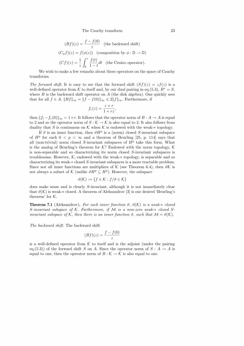
(Bf)(z) =f − f(0)

z(the backward shift)

(Cφf)(z) = f(φ(z)) (composition by φ : D→ D)

(Cf)(z) =1z

∫ z

0

f(t)1− t

dt (the Cesaro operator).

We wish to make a few remarks about these operators on the space of Cauchytransforms.

The forward shift. It is easy to see that the forward shift (Sf)(z) = zf(z) is awell-defined operator from K to itself and, by our dual pairing in eq.(5.3), B∗ = S,where B is the backward shift operator on A (the disk algebra). One quickly seesthat for all f ∈ A, ‖Bf‖∞ = ‖f − f(0)‖∞ 6 2‖f‖∞. Furthermore, if

fr(z) =z + r

1 + rz,

then ‖fr−fr(0)‖∞ = 1+r. It follows that the operator norm of B : A→ A is equalto 2 and so the operator norm of S : K → K is also equal to 2. It also follows fromduality that S is continuous on K when K is endowed with the weak-∗ topology.

If ϑ is an inner function, then ϑHp is a (norm) closed S-invariant subspaceof Hp for each 0 < p < ∞ and a theorem of Beurling [25, p. 114] says thatall (non-trivial) norm closed S-invariant subspaces of Hp take this form. Whatis the analog of Beurling’s theorem for K? Endowed with the norm topology, Kis non-separable and so characterizing its norm closed S-invariant subspaces istroublesome. However, K, endowed with the weak-∗ topology, is separable and socharacterizing its weak-∗ closed S-invariant subspaces is a more tractable problem.Since not all inner functions are multipliers of K (see Theorem 6.4), then ϑK isnot always a subset of K (unlike ϑHp ⊆ Hp). However, the subspace

ϑ(K) := f ∈ K : f/ϑ ∈ K

does make sense and is clearly S-invariant, although it is not immediately clearthat ϑ(K) is weak-∗ closed. A theorem of Aleksandrov [3] is our desired ‘Beurling’stheorem’ for K.

Theorem 7.1 (Aleksandrov). For each inner function ϑ, ϑ(K) is a weak-∗ closedS-invariant subspace of K. Furthermore, if M is a non-zero weak-∗ closed S-invariant subspace of K, then there is an inner function ϑ, such that M = ϑ(K).

The backward shift. The backward shift

(Bf)(z) =f − f(0)

z

is a well-defined operator from K to itself and is the adjoint (under the pairingeq.(5.3)) of the forward shift S on A. Since the operator norm of S : A → A isequal to one, then the operator norm of B : K → K is also equal to one.


The space Ka = f+ : f ∈ L1 is the norm closure of the polynomials andhence is separable. A theorem of Aleksandrov [3] (see also [16, p. 99]) characterizesthe B-invariant subspaces of Ka.

Theorem 7.2 (Aleksandrov). If M is a norm closed B-invariant subspace of Ka,then there is an inner function ϑ such that f ∈ M if and only if there is aG ∈ N+(De) with G(∞) = 0 and such that

limr→1−

f

ϑ(rζ) = lim

r→1−G(ζ/r)

for m-almost every ζ ∈ T.

The function G is known in the literature as a ‘pseudocontinuation’ of thefunction f/ϑ (see [75] for more on pseudocontinuations). We compare Aleksan-drov’s result to the characterization of the backward shift invariant subspaces ofH2 which, as mentioned in the introduction, are all of the form (ϑH2)⊥. A theo-rem of Douglas-Shapiro-Shields [24] says that f ∈ (ϑH2)⊥ if and only if there isa function G ∈ H2(De), with G(∞) = 0, such that G is a pseudocontinuation off/ϑ, i.e., G (from the outside of the disk) has the same radial limits as f/ϑ (fromthe inside of the disk) almost everywhere.

For a weak-∗ closed B-invariant subspace N ⊆ K, the dual pairing eq.(5.3)tells us that N⊥ (the pre-annihilator of N ) is an S-invariant subspace of A. Since Ais a Banach algebra and polynomials are dense in A, then N⊥ is a closed ideal of A.A result of Rudin [76] (see also [40, p. 82]) characterizes these ideals by their innerfactors and their zero sets on the circle. A result in [15] uses the Rudin characteri-zation to describe the corresponding N using analytic continuation across certainportions of the circle. This result also has connections to an analytic continuationresult of Korenblum [52]. Some partial results on the B-invariant subspaces of K,when endowed with the norm topology, can be found in [15].

Composition operators. For an analytic map φ : D → D, define, for a Cauchytransform f , the function

(Cφf)(z) = f(φ(z)).

Clearly Cφf is an analytic function on D. What is not immediately clear is thatCφf is a Cauchy transform. The proof of this follows from the Herglotz theorem[25, p. 2] and the decomposition of any measure as the complex linear sum of fourpositive measures. Furthermore, we note that if G is simply connected and theRiemann map g : D → G belongs to K, then any analytic map f of D into Gbelongs to K. Indeed, set φ = g−1 f and notice that f = Cφg ∈ K. Finally, if fis analytic on D and C \ f(D) contains at least two oppositely oriented half-lines,then f ∈ K [12].


Without too much difficulty, one can show that Cφ has closed graph and soCφ is bounded on K. Bourdon and Cima [12] proved that

‖Cφ‖ 62 + 2

√2

1− |φ(0)|which was improved to

‖Cφ‖ 61 + 2|φ(0)|1− |φ(0)|

by Cima and Matheson [14]. Moreover, equality is attained for certain linear frac-tional maps φ.

The theory of Clark measures, as discussed in § 1, leads us to a characteriza-tion of the compact composition operators on K. Following Sarason, for each selfmap φ : D→ D, we define an operator on M as follows: For µ in M+ the function(Pµ)(z), the Poisson integral of the measure µ, is positive and harmonic in D.Hence, the function v(z) = (Pµ)(φ(z)) is also positive and harmonic. By the Her-glotz theorem there is ν ∈M+ with v(z) = (Pν)(z). Let Sφ(µ) = ν, where ν is the(positive) measure for which (Pν)(z) = (Pµ)(φ(z)). Extended Sφ linearly to all ofM in the obvious way (writing every measure as a complex linear combination offour positive measures).

Theorem 7.3 (Sarason [81]). The operator Sφ is compact if and only if each Clarkmeasure µα associated with φ satisfies µα m for all α ∈ T. Moreover, Sφ mapsL1 continuously to L1.

We comment that Sarason’s result is equivalent to J. Shapiro’s condition forcompactness on H2 [14, 83]. Also worth noting is that if the map φ is inner, it cannot induce a compact operator in this setting, since the Clark measure σα will becarried by φ = α, and hence is singular. Using these results, one can show thefollowing [14].

Theorem 7.4. Let φ be an analytic self map of the disk. Then

1. Cφ is compact on K if and only if Sφ is compact on M.2. if Cφ is weakly compact on K, then Cφ is compact on K.

The Cesaro operator. The Cesaro operator, as it originally appeared in the operatorsetting, was simply the map defined on the sequence space (`2)+ by

(an)n>0 → (bN )N>0,

where

bN :=1

N + 1(a0 + a1 + · · ·+ aN

), N = 0, 1, 2, . . .

is the N -th Cesaro mean of the sequence (an)n>0. It is easy to see, equating the `2

sequence (an)n>0 with the H2 function f =∑anz

n, that this operator, denoted


by C, can be viewed on H2 as the integral operator

(Cf)(z) :=1z

∫ z

0

f(t)(1− t)

dt.

Cima and Siskakis [17] prove that the Cesaro operator is continuous from K to K.An interesting problem to consider is whether or not any of the generalized Cesarooperators on Hp considered in [6, 7] are continuous on K.

8. Distribution of boundary values

For a measurable (with respect to normalized Lebesgue measure m) function f onT, the distribution function

λ→ m(|f | > λ)

is seen throughout analysis. For example, there is Chebyshev’s inequality

m(|f | > λ) 61λp‖f‖p

and the ’layer cake representation’ formula

‖f‖pp = p

∫ ∞

0

λp−1m(|f | > λ)dλ.

In this brief section, we mention some known results about the distribution func-tions for Kµ and Qµ and how they relate in quite surprising ways to µ.

Perhaps the earliest result on the distribution function for Qµ is one of G.Boole [11] who in 1857 found, in the special case where µ is a finite positive linearcombination of point masses, the exact formula

m(Qµ > λ) = m(Qµ < −λ) =1π

arctan‖µ‖λ.

Although, for positive measures with an absolutely continuous component(i.e., dµ/dm 6≡ 0), Boole’s formula is not true, it is ‘asymptotically true’ as morerecent results of Tsereteli [94] and Poltoratski [66] show.

Theorem 8.1 (Poltoratski). Let µ ∈M+ and Eµ = ζ ∈ T :dµ

dm(ζ) > 0. Then

1π

arctan‖µ‖λ

−m(Eµ) 6 m(Qµ > λ \ Eµ) 61π

arctan‖µ‖λ,

1π

arctan‖µ‖λ

−m(Eµ) 6 m(Qµ < −λ \ Eµ) 61π

arctan‖µ‖λ.

The above theorem is an improvement of [94]. Another fascinating aspectof Qµ (and hence Kµ) is a result of Stein and Weiss [92] (see also [48, p. 71])which says that if χU is the characteristic function of some set U ⊂ T, then thedistribution function forQ(χUdm) depends only onm(U) and not on the particulargeometric structure of U .


The next series of results deal with reproducing the singular part of a measurefrom knowledge of the distribution function for Qµ (or Kµ). Probably one of theearliest of such theorems is this one of Hruscev and Vinogradov [43].

Theorem 8.2 (Hruscev and Vinogradov). For any µ ∈M ,

limλ→∞

πλm(|Kµ| > λ) = ‖µs‖.

Note that if µ m, then we get the well-known estimate (see eq.(3.8))

m(|Kµ| > λ) = o(1/λ).

Recent work of Poltoratski [66] says that not only can one recover the total varia-tion norm of µs from the distribution function for Kµ, but one can actually recoverthe measure µs. For any measure µ ∈M decomposed as µ = (µ1−µ2)+i(µ3−µ4),where µj > 0, let |µ| be the measure |µ| :=

∑4j=1 µj .

Theorem 8.3 (Poltoratski). For µ ∈ M , the measure πλχ|Kµ|>λ · m convergesweak-∗ to |µs| as λ→∞.

Though we don’t have time to go into the details, we do mention that at theheart of these Poltoratski theorems is the Aleksandrov conditional expectationoperator and the relationship between the distribution functions for Qµ and Kµand Clark measures (as described in §1).

9. The normalized Cauchy transform

If σα is a Clark measure for the inner function ϑ, the adjoint F∗α of the unitary

operator Fα : (ϑH2)⊥ → L2(σα) (as described in §1) is

F∗αf =

K(f dσα)K(σα)

In general, for µ ∈M+ we can consider the normalized Cauchy transform

Vµf =K(f dµ)K(µ)

, f ∈ L1(µ).

This transform has been studied by several authors, beginning with D. Clark [18],with significant contributions by Aleksandrov [4] and Poltoratski [65, 66, 67].

In this section we wish to describe some recent work of Poltoratski on maximalproperties of this normalized transform. Poltoratski’s motivation for this study isthe famous theorem of Hunt, Muckenhoupt, and Wheeden [29, p. 255] [45], whichstates that the Cauchy transform is bounded on Lp(w), 1 < p <∞, if and only if wis an ‘Ap-weight’. Moreover, if MKf denotes the standard nontangential maximalfunction of the Cauchy transform Kf , we have similarly MKf ∈ Lp(w) for allf ∈ Lp(w) if and only if w is an Ap-weight.

We can ask about the behavior of the normalized Cauchy transform Vµ andthe associated maximal operator MVµ on Lp(µ). We first note that Vµ is alwaysbounded on L2(µ). In fact if µ = m, then Vµ(L2(µ)) is just the Hardy space H2,


while if µ is singular Vµ(L2(µ)) = (ϑH2)⊥, where ϑ is the inner function relatedto µ by the formula

Kµ =1

1− ϑ.

If µ is an arbitrary positive measure, Vµ(L2(µ)) is the de Branges-Rovnyak spaceMϑ, where ϑ comes from the above formula, but is no longer inner [82]. In par-ticular, Vµ is a bounded operator from L2(µ) to H2 for any µ ∈M+. When p 6= 2the situation is described by the following theorem of Aleksandrov [5].

Theorem 9.1. For any µ ∈ M+, Vµ is a bounded operator from Lp(µ) to Hp for1 2. If µ is singular and Vµ is boundedfrom Lp(µ) to Hp, then µ is a discrete measure.

The following theorem of Poltoratski [65] describes the boundary behavior ofVµf .

Theorem 9.2. Let µ ∈ M+ and f ∈ L1(µ). Then the function Vµf has finitenontangential boundary values µ-a.e. These values coincide with f µs-a.e.

The above result shows in particular that if µ is singular, then Vµ is in factthe identity operator on L1(µ), and so is certainly a bounded operator from Lp(µ)to itself. The situation for arbitrary µ and for the maximal operator MVµ is moreinvolved and was examined by the following theorem of Poltoratski [68].

Theorem 9.3. For any µ ∈ M+, Vµ is a bounded operator from Lp(µ) to itselffor 1 < p 6 2. In addition, the maximal operator MVµ is bounded on Lp(µ) for1 < p < 2, and of weak type (2, 2) on L2(µ).

Even for singular µ, the maximal operator MVµ may be unbounded. Indeed,Poltoratski provides an example of a singular measure µ and an f ∈ L∞(µ) suchthat MVµf 6∈ Lp(µ) for any p > 2. Finally, although MVµ is always of weak type(2, 2), it is not known whether or not it is bounded on L2(µ) in general. It is alsonot known under what conditions it is of weak type (1, 1).

References

1. A. B. Aleksandrov, A-integrability of boundary values of harmonic functions, Mat.Zametki 30 (1981), no. 1, 59–72, 154. MR 83j:30039

2. , Essays on nonlocally convex Hardy classes, Complex analysis and spectraltheory (Leningrad, 1979/1980), Springer, Berlin, 1981, pp. 1–89. MR 84h:46066

3. , Invariant subspaces of shift operators. An axiomatic approach, Zap. Nauchn.Sem. Leningrad. Otdel. Mat. Inst. Steklov. (LOMI) 113 (1981), 7–26, 264, Investi-gations on linear operators and the theory of functions, XI. MR 83g:47031

4. , Multiplicity of boundary values of inner functions, Izv. Akad. Nauk Armyan.SSR Ser. Mat. 22 (1987), no. 5, 490–503, 515. MR 89e:30058


5. , Inner functions and related spaces of pseudocontinuable functions, Zap.Nauchn. Sem. Leningrad. Otdel. Mat. Inst. Steklov. (LOMI) 170 (1989), no. Issled.Linein. Oper. Teorii Funktsii. 17, 7–33, 321. MR 91c:30063

6. A. Aleman and J. Cima, An integral operator on Hp and Hardy’s inequality, J. Anal.Math. 85 (2001), 157–176. MR 1 869 606

7. A. Aleman and A. Siskakis, An integral operator on Hp, Complex Variables TheoryAppl. 28 (1995), no. 2, 149–158. MR 2000d:47050

8. N. K. Bary, A treatise on trigonometric series. Vols. I, II, Authorized translationby Margaret F. Mullins. A Pergamon Press Book, The Macmillan Co., New York,1964. MR 30 #1347

9. S. Bell, The Cauchy transform, potential theory, and conformal mapping, CRC Press,Boca Raton, FL, 1992. MR 94k:30013

10. S. V. Bockarev, Existence of a basis in the space of functions analytic in the disc,and some properties of Franklin’s system, Mat. Sb. (N.S.) 95(137) (1974), 3–18, 159.MR 50 #8036

11. G. Boole, On the comparison of transcendents with certain applications to the theoryof definite integrals, Phil. Trans. Royal Soc. 147 (1857), 745–803.

12. P. Bourdon and J. A. Cima, On integrals of Cauchy-Stieltjes type, Houston J. Math.14 (1988), no. 4, 465–474. MR 90h:30095

13. L. Brown and A. L. Shields, Cyclic vectors in the Dirichlet space, Trans. Amer.Math. Soc. 285 (1984), no. 1, 269–303. MR 86d:30079

14. J. A. Cima and A. Matheson, Cauchy transforms and composition operators, IllinoisJ. Math. 42 (1998), no. 1, 58–69. MR 98k:42028

15. J. A. Cima, A. Matheson, and W. T. Ross, The backward shift on the space ofCauchy transforms, to appear, Proc. Amer. Math. Soc.

16. J. A. Cima and W. T. Ross, The backward shift on the Hardy space, AmericanMathematical Society, Providence, RI, 2000. MR 2002f:47068

17. J. A. Cima and A. Siskakis, Cauchy transforms and Cesaro averaging operators,Acta Sci. Math. (Szeged) 65 (1999), no. 3-4, 505–513. MR 2000m:47043

18. D. Clark, One dimensional perturbations of restricted shifts, J. Analyse Math. 25(1972), 169–191. MR 46 #692

19. B. Davis, On the distributions of conjugate functions of nonnegative measures, DukeMath. J. 40 (1973), 695–700. MR 48 #2649

20. , On the weak type (1, 1) inequality for conjugate functions, Proc. Amer.Math. Soc. 44 (1974), 307–311. MR 50 #879

21. , On Kolmogorov’s inequalities fp ≤ Cp f1, 0 < p < 1, Trans. Amer. Math.Soc. 222 (1976), 179–192. MR 54 #10967

22. F. Delbaen, Weakly compact operators on the disc algebra, J. Algebra 45 (1977),no. 2, 284–294. MR 58 #2304

23. J. Diestel, Sequences and series in Banach spaces, Springer-Verlag, New York, 1984.MR 85i:46020

24. R. G. Douglas, H. S. Shapiro, and A. L. Shields, Cyclic vectors and invariant sub-spaces for the backward shift operator., Ann. Inst. Fourier (Grenoble) 20 (1970),no. fasc. 1, 37–76. MR 42 #5088


25. P. L. Duren, Theory of Hp spaces, Academic Press, New York, 1970. MR 42 #3552

26. P. Fatou, Series trigonometriques et series de Taylor, Acta Math. 30 (1906), 335 –400.

27. O. Frostman, Sur les produits de Blaschke, Kungl. Fysiografiska Sallskapets i LundForhandlingar [Proc. Roy. Physiog. Soc. Lund] 12 (1942), no. 15, 169–182. MR6,262e

28. J. B. Garnett, Analytic capacity and measure, Springer-Verlag, Berlin, 1972, LectureNotes in Mathematics, Vol. 297. MR 56 #12257

29. , Bounded analytic functions, Academic Press Inc., New York, 1981. MR83g:30037

30. V. V. Golubev, Single valued analytic functions with perfect sets of singular points,Ph.D. thesis, Moscow, 1917.

31. G. M. Goluzin, Geometric theory of functions of a complex variable, American Math-ematical Society, Providence, R.I., 1969. MR 40 #308

32. G. H. Hardy and J. E. Littlewood, Some more theorems concerning Fourier seriesand Fourier power series, Duke Math. J. 2 (1936), 354 – 382.

33. V. P. Havin, On analytic functions representable by an integral of Cauchy-Stieltjestype, Vestnik Leningrad. Univ. Ser. Mat. Meh. Astr. 13 (1958), no. 1, 66–79. MR20 #1762

34. , Analytic representation of linear functionals in spaces of harmonic andanalytic functions which are continuous in a closed region, Dokl. Akad. Nauk SSSR151 (1963), 505–508. MR 27 #2636

35. , The spaces H∞ and L1/H10 , Zap. Naucn. Sem. Leningrad. Otdel. Mat.

Inst. Steklov. (LOMI) 39 (1974), 120–148, Investigations on linear operators andthe theory of functions, IV. MR 50 #965

36. S. Ya. Havinson, On an extremal problem of the theory of analytic functions, UspehiMatem. Nauk (N.S.) 4 (1949), no. 4(32), 158–159. MR 11,508e

37. , On some extremal problems of the theory of analytic functions, Moskov.Gos. Univ. Ucenye Zapiski Matematika 148(4) (1951), 133–143. MR 14,155f

38. H. Helson and G. Szego, A problem in prediction theory, Ann. Mat. Pura Appl. (4)51 (1960), 107–138. MR 22 #12343

39. E. Hewitt and K. Stromberg, Real and abstract analysis. A modern treatment ofthe theory of functions of a real variable, Springer-Verlag, New York, 1965. MR 32#5826

40. K. Hoffman, Banach spaces of analytic functions, Dover Publications Inc., New York,1988, Reprint of the 1962 original. MR 92d:46066

41. B. Hollenbeck and I. Verbitsky, Best constants for the Riesz projection, J. Funct.Anal. 175 (2000), no. 2, 370–392. MR 2001i:42010

42. S. V. Hruscev, The problem of simultaneous approximation and of removal of thesingularities of Cauchy type integrals, Trudy Mat. Inst. Steklov. 130 (1978), 124–195,223, Spectral theory of functions and operators. MR 80j:30055

43. S. V. Hruscev and S. A. Vinogradov, Free interpolation in the space of uniformly con-vergent Taylor series, Complex analysis and spectral theory (Leningrad, 1979/1980),Springer, Berlin, 1981, pp. 171–213. MR 83b:30032


44. , Inner functions and multipliers of Cauchy type integrals, Ark. Mat. 19(1981), no. 1, 23–42. MR 83c:30027

45. R. Hunt, B. Muckenhoupt, and R. Wheeden, Weighted norm inequalities for theconjugate function and Hilbert transform, Trans. Amer. Math. Soc. 176 (1973), 227–251. MR 47 #701

46. J.-P. Kahane, Best approximation in L1(T ), Bull. Amer. Math. Soc. 80 (1974), 788–804. MR 52 #3845

47. S. Kakutani, Concrete representation of abstract (L)-spaces and the mean ergodictheorem, Ann. of Math. (2) 42 (1941), 523–537. MR 2,318d

48. Y. Katznelson, An introduction to harmonic analysis, corrected ed., Dover Publica-tions Inc., New York, 1976. MR 54 #10976

49. S. V. Kisljakov, The Dunford-Pettis, Pe lczynski and Grothendieck conditions, Dokl.Akad. Nauk SSSR 225 (1975), no. 6, 1252–1255. MR 53 #1241

50. A. N. Kolmogorov, Sur les fonctions harmoniques conjuquees et les series de Fourier,Fund. Math. 7 (1925), 24 – 29.

51. P. Koosis, Introduction to Hp spaces, second ed., Cambridge University Press, Cam-bridge, 1998. MR 2000b:30052

52. B. I. Korenblum, Closed ideals of the ring An, Funkcional. Anal. i Prilozen. 6 (1972),no. 3, 38–52. MR 48 #2776

53. P. I. Kuznetsov and E. D. Solomentsev, Ivan Ivanovich Privalov (on the ninetiethanniversary of his birth), Uspekhi Mat. Nauk 37 (1982), no. 4(226), 193–211 (1plate). MR 84b:01049

54. A. I. Markushevich, Theory of functions of a complex variable. Vol. I, II, III, Englished., Chelsea Publishing Co., New York, 1977. MR 56 #3258

55. L. A. Markushevich and G. Ts. Tumarkin, On a class of functions that can berepresented in a domain by an integral of Cauchy-Stieltjes type, Uspekhi Mat. Nauk52 (1997), no. 3(315), 169–170. MR 98j:30045

56. V. G. Maz′ya and T. O. Shaposhnikova, Theory of multipliers in spaces of differen-tiable functions, Pitman (Advanced Publishing Program), Boston, MA, 1985. MR87j:46074

57. M. Mooney, A theorem on bounded analytic functions, Pacific J. Math. 43 (1972),457–463. MR 47 #2374

58. N. I. Muskhelishvili, Singular integral equations, Dover Publications Inc., New York,1992, Boundary problems of function theory and their application to mathematicalphysics, Translated from the second (1946) Russian edition and with a preface byJ. R. M. Radok, Corrected reprint of the 1953 English translation. MR 94a:45001

59. D. J. Newman, The nonexistence of projections from L1 to H1, Proc. Amer. Math.Soc. 12 (1961), 98–99. MR 22 #11276

60. N. K. Nikol′skiı, Treatise on the shift operator, Springer-Verlag, Berlin, 1986. MR87i:47042

61. H. Pajot, Analytic capacity, rectifiability, Menger curvature and the Cauchy integral,Lecture Notes in Mathematics, vol. 1799, Springer-Verlag, Berlin, 2002. MR 1 952175


62. A. Pe lczynski, Banach spaces of analytic functions and absolutely summing oper-ators, American Mathematical Society, Providence, R.I., 1977, Expository lecturesfrom the CBMS Regional Conference held at Kent State University, Kent, Ohio, July11–16, 1976, Conference Board of the Mathematical Sciences Regional ConferenceSeries in Mathematics, No. 30. MR 58 #23526

63. S. K. Pichorides, On the best values of the constants in the theorems of M. Riesz,Zygmund and Kolmogorov, Studia Math. 44 (1972), 165–179. (errata insert), Collec-tion of articles honoring the completion by Antoni Zygmund of 50 years of scientificactivity, II. MR 47 #702

64. J. Plemelj, Ein Erganzungssatz zur Cauchyschen Integraldarstellung analytischerFunctionen, Randwerte betreffend, Monatshefte fur Math. u. Phys. XIX (1908), 205– 210.

65. A. Poltoratski, Boundary behavior of pseudocontinuable functions, Algebra i Analiz5 (1993), no. 2, 189–210. MR 94k:30090

66. , On the distributions of boundary values of Cauchy integrals, Proc. Amer.Math. Soc. 124 (1996), no. 8, 2455–2463. MR 96j:30057

67. , Kreın’s spectral shift and perturbations of spectra of rank one, Algebra iAnaliz 10 (1998), no. 5, 143–183. MR 2000d:47028

68. , Maximal properties of the normalized Cauchy transform, J. Amer. Math.Soc. 16 (2003), no. 1, 1–17 (electronic). MR 2003j:30056

69. I. I. Privalov, Sur les fonctions conjuguees, Bull. Soc. Math. France 44 (1916), 100–103.

70. , Integral de Cauchy, Ph.D. thesis, Saratov, 1919.

71. , Randeigenschaften analytischer Funktionen, VEB Deutscher Verlag derWissenschaften, Berlin, 1956. MR 18,727f

72. F. Riesz and M. Riesz, Uber die Randwerte einer analytischen Function, IV Skand.Math. Kongr., Mittag-Leffler, Uppsala (1920), 27–44.

73. M. Riesz, Sur les fonctions conjugees, Math. Z. 27 (1927), 218 – 244.

74. W. W. Rogosinski and H. S. Shapiro, On certain extremum problems for analyticfunctions, Acta Math. 90 (1953), 287–318. MR 15,516a

75. W. T. Ross and H. S. Shapiro, Generalized analytic continuation, University Lec-ture Series, vol. 25, American Mathematical Society, Providence, RI, 2002. MR2003h:30003

76. W. Rudin, The closed ideals in an algebra of analytic functions, Canad. J. Math. 9(1957), 426–434. MR 19,641c

77. , Real and complex analysis, third ed., McGraw-Hill Book Co., New York,1987. MR 88k:00002

78. , Functional analysis, second ed., McGraw-Hill Inc., New York, 1991. MR92k:46001

79. A. Rybkin, On an analogue of Cauchy’s formula for Hp, 1/2 ≤ p < 1, and theCauchy type integral of a singular measure, Complex Variables Theory Appl. 43(2000), no. 2, 139–149. MR 2001i:30042

80. D. Sarason, Functions of vanishing mean oscillation, Trans. Amer. Math. Soc. 207(1975), 391–405. MR 51 #13690


81. , Composition operators as integral operators, Analysis and partial differentialequations, Dekker, New York, 1990, pp. 545–565. MR 92a:47040

82. , Sub-Hardy Hilbert spaces in the unit disk, University of Arkansas LectureNotes in the Mathematical Sciences, 10, John Wiley & Sons Inc., New York, 1994,A Wiley-Interscience Publication. MR 96k:46039

83. J. Shapiro and C. Sundberg, Compact composition operators on L1, Proc. Amer.Math. Soc. 108 (1990), no. 2, 443–449. MR 90d:47035

84. N. A. Shirokov, Analytic functions smooth up to the boundary, Springer-Verlag,Berlin, 1988. MR 90h:30087

85. V. I. Smirnov, Sur les valeurs limites des fonctions, regulieres a l’interieur d’uncercle, Journal de la Societe Phys.-Math. de Leningrade 2 (1929), 22–37.

86. F. Smithies, Cauchy and the creation of complex function theory, Cambridge Uni-versity Press, Cambridge, 1997. MR 99b:01013

87. Yu. B. Sokhotskii, On definite integrals and functions using series expansions, Ph.D.thesis, St. Petersburg, 1873.

88. S. Spanne, Sur l’interpolation entre les espaces LkpΦ, Ann. Scuola Norm. Sup. Pisa

(3) 20 (1966), 625–648. MR 35 #728

89. D. Stegenga, Multipliers of the Dirichlet space, Illinois J. Math. 24 (1980), no. 1,113–139. MR 81a:30027

90. E. M. Stein, Singular integrals, harmonic functions, and differentiability propertiesof functions of several variables, Singular integrals (Proc. Sympos. Pure Math.,Chicago, Ill., 1966), Amer. Math. Soc., Providence, R.I., 1967, pp. 316–335. MR 58#2467

91. , Singular integrals and differentiability properties of functions, PrincetonMathematical Series, No. 30, Princeton University Press, Princeton, N.J., 1970.MR 44 #7280

92. E. M. Stein and G. Weiss, An extension of a theorem of Marcinkiewicz and some ofits applications, J. Math. Mech. 8 (1959), 263–284. MR 21 #5888

93. O. D. Tsereteli, Remarks on the theorems of Kolmogorov and of F. and M. Riesz,Proceedings of the Symposium on Continuum Mechanics and Related Problemsof Analysis (Tbilisi, 1971), Vol. 1 (Russian), Izdat. “Mecniereba”, Tbilisi, 1973,pp. 241–254. MR 52 #6306

94. , Conjugate functions, Mat. Zametki 22 (1977), no. 5, 771–783. MR 58#12166

95. G. C. Tumarkin, On integrals of Cauchy-Stieltjes type, Uspehi Mat. Nauk (N.S.) 11(1956), no. 4(70), 163–166. MR 18,725f

96. P. L. Ul′yanov, On the A-Cauchy integral. I, Uspehi Mat. Nauk (N.S.) 11 (1956),no. 5(71), 223–229. MR 18,726a

97. S. A. Vinogradov, Properties of multipliers of integrals of Cauchy-Stieltjes type, andsome problems of factorization of analytic functions, Mathematical programmingand related questions (Proc. Seventh Winter School, Drogobych, 1974), Theory of

functions and functional analysis (Russian), Central Ekonom.-Mat. Inst. Akad. NaukSSSR, Moscow, 1976, pp. 5–39. MR 58 #28518


98. S. A. Vinogradov, M. G. Goluzina, and V. P. Havin, Multipliers and divisorsof Cauchy-Stieltjes type integrals, Zap. Naucn. Sem. Leningrad. Otdel. Mat. Inst.Steklov. (LOMI) 19 (1970), 55–78. MR 45 #562

99. P. Wojtaszczyk, Banach spaces for analysts, Cambridge University Press, Cam-bridge, 1991. MR 93d:46001

100. A. Zygmund, Sur les fonctions conjugees, Fund. Math. 13 (1929), 284 – 303.

101. , Trigonometric series. 2nd ed. Vols. I, II, Cambridge University Press, NewYork, 1959. MR 21 #6498

Department of Mathematics, University of North Carolina, Chapel Hill, NorthCarolina 27599E-mail address: [email protected]

Department of Mathematics, Lamar University, Beaumont, Texas 77710E-mail address: [email protected]

Department of Mathematics and Computer Science, University of Richmond, Rich-mond, Virginia 23173E-mail address: [email protected]

Date post:	13-May-2018
Category:	Documents
Upload:	ngodien
View:	216 times
Download:	1 times

The Cauchy transform - University of Richmondwross/PDF/cauchy.pdf · The Cauchy transform Joseph A....

Documents