The Causal Impact of Common Native Language on International Trade: Evidence from a Spatial Regression Discontinuity Design * Peter H. Egger and Andrea Lassmann October 10, 2013 * Acknowledgements: We thank the Swiss Federal Customs Administration for generously pro- viding data on trade transactions and the Swiss Federal Statistical Office for providing data on language use. We further thank Raphael Auer, Christoph Basten, Claudia Bernasconi, Paola Conconi, Andreas Fischer, Taiji Furusawa, Victor Ginsburgh, James Harrigan, Jota Ishikawa, Michaela Kesina, Veronika Killer, Mariko Klasing, Jacob LaRiviere, Thierry Mayer, Jacques Melitz, William S. Neilson, Harald Oberhofer, Emanuel Ornelas, Rapha¨ el Parchet, Mathieu Parenti, Philip Saur´ e, Georg Schaur, Jan Schymik, Ren´ e Sieber, Daniel Sturm, Mathias Thoenig, Farid Toubal, Christian Volpe Martincus, and Hannes Winner for numerous useful comments. We benefited from comments of participants at the Annual Conference of the Canadian Economics Association 2011, the SSES Annual Meeting 2011, the 26th Annual European Economic Association Congress 2011, European Trade Study Group 2011, the Young Swiss Economists Meeting 2012, the Spring Meeting of Young Economists 2012, the Annual Meeting of the Austrian Economic Association 2012, the Brixen Workshop & Summer School on International Trade and Finance 2012, the HSE Center for Market Studies and Spatial Economics at St. Petersburg 2012, the Heriot-Watt University at Edinburgh 2012, the Inter-American Development Bank 2012, the Swiss National Bank 2012, the University of Heidelberg 2013, the University of Tennessee at Knoxville 2012, the CEPR Conference on Causal Analysis in International Trade 2013, the Hitotsubashi University Winter International Trade Seminar, the University of Salzburg 2013, the London School of Economics 2013, and the 13th Research in International Trade and International Finance meetings at Paris I University 2013. Egger : ETH Zurich (KOF Swiss Economic Institute), CEPR, CESifo, WIFO; Email: eg- [email protected]. Lassmann : ETH Zurich (KOF Swiss Economic Institute); Email: lass- [email protected]; Address: KOF Swiss Economic Institute, WEH D4, Weinbergstrasse 35, 8092 Zurich, Switzerland.
Transcript
The Causal Impact of Common Native Language on
International Trade: Evidence from a Spatial Regression
Discontinuity Design∗
Peter H. Egger and Andrea Lassmann
October 10, 2013
∗Acknowledgements: We thank the Swiss Federal Customs Administration for generously pro-viding data on trade transactions and the Swiss Federal Statistical Office for providing data onlanguage use. We further thank Raphael Auer, Christoph Basten, Claudia Bernasconi, PaolaConconi, Andreas Fischer, Taiji Furusawa, Victor Ginsburgh, James Harrigan, Jota Ishikawa,Michaela Kesina, Veronika Killer, Mariko Klasing, Jacob LaRiviere, Thierry Mayer, Jacques Melitz,William S. Neilson, Harald Oberhofer, Emanuel Ornelas, Raphael Parchet, Mathieu Parenti, PhilipSaure, Georg Schaur, Jan Schymik, Rene Sieber, Daniel Sturm, Mathias Thoenig, Farid Toubal,Christian Volpe Martincus, and Hannes Winner for numerous useful comments. We benefited fromcomments of participants at the Annual Conference of the Canadian Economics Association 2011,the SSES Annual Meeting 2011, the 26th Annual European Economic Association Congress 2011,European Trade Study Group 2011, the Young Swiss Economists Meeting 2012, the Spring Meetingof Young Economists 2012, the Annual Meeting of the Austrian Economic Association 2012, theBrixen Workshop & Summer School on International Trade and Finance 2012, the HSE Centerfor Market Studies and Spatial Economics at St. Petersburg 2012, the Heriot-Watt University atEdinburgh 2012, the Inter-American Development Bank 2012, the Swiss National Bank 2012, theUniversity of Heidelberg 2013, the University of Tennessee at Knoxville 2012, the CEPR Conferenceon Causal Analysis in International Trade 2013, the Hitotsubashi University Winter InternationalTrade Seminar, the University of Salzburg 2013, the London School of Economics 2013, and the13th Research in International Trade and International Finance meetings at Paris I University 2013.Egger : ETH Zurich (KOF Swiss Economic Institute), CEPR, CESifo, WIFO; Email: [email protected]. Lassmann: ETH Zurich (KOF Swiss Economic Institute); Email: [email protected]; Address: KOF Swiss Economic Institute, WEH D4, Weinbergstrasse 35, 8092Zurich, Switzerland.
Abstract
This paper studies the causal effect of sharing a common native languageon international trade. Switzerland is a multilingual country that hosts fourofficial language groups of which three are major (French, German, and Italian).These groups of native language speakers are geographically separated, with thecorresponding regions bordering countries which share a majority of speakersof the same native language. All of the three main languages are understoodand spoken by most Swiss citizens, especially the ones residing close to internallanguage borders in Switzerland. This unique setting allows for an assessmentof the impact of common native (rather than spoken) language as a culturalaspect of language on trade from within country-pairs. We do so by exploitingthe discontinuity in various international bilateral trade outcomes based onSwiss transaction-level data at historical language borders within Switzerland.The effect on various margins of imports is positive and significant. Theresults suggest that, on average, common native language between regionsbiases the regional structure of the value of international imports towardsthem by 18 percentage points and that of the number of import transactionsby 20 percentage points. In addition, regions import 102 additional productsfrom a neighboring country sharing a common native language compared to adifferent native language exporter. This effect is considerably lower than theoverall estimate (using aggregate bilateral trade and no regression discontinuitydesign) of common official language on Swiss international imports in the samesample. The latter subsumes both the effect of common spoken language as acommunication factor and of confounding economic and institutional factorsand is quantitatively well in line with the common official (spoken or native)language coefficient in many gravity model estimates of international trade.
Keywords: Common language; Culture; International trade;Regression discontinuity design; Quasi-randomized experimentsJEL Classification: C14, C21, F14, R12, Z10
1 Introduction
This paper revolves around three pertinent questions in economics. First, why isconsumption so much biased towards domestic goods? Second, why are importsso much biased towards similar countries? Third, what is the economic value ofcommon culture?1 The question of key interest to this paper is to which extentcommon language as a measure cultural proximity affects international trade.
The overall quantitative effect (and even the channels of influence) of a commonlanguage on trade is well studied in empirical international economics. Tradeeconomists usually estimate the impact of common language on bilateral trade fromgravity model regressions of the following general form:
Mij = eλlanguageijdijµimjuij, (1)
where Mij measures bilateral trade (imports) of country j from country i, languageijis a binary indicator variable which is unity whenever two countries have the sameofficial language and zero else, λ is an unknown but estimable parameter on languageij ,dij is the joint impact of other measurable bilateral trade-impeding or trade-enhancingfactors (such as bilateral distance or trade agreement membership) on bilateral trade,µi and mj are exporter- and importer-specific factors of influence (such as GDP, priceindices, etc.), and uij is a country-pair-specific error term. λ should be interpreted asa direct effect of common language on bilateral trade in terms of a semi-elasticity.2 Akey problem with this identification strategy is that λ may be biased due to omittedconfounding cultural, institutional, and political factors in uij beyond the usuallyemployed trade cost variables in dij that are correlated with languageij (see Eggerand Lassmann, 2012, for a meta-analysis of the common language effect on trade
1The first question is one of Obstfeld and Rogoff’s (2001) six major puzzles in internationalmacroeconomics. The second one is the very root of new trade theory as developed in Krugman(1980). The last question is at the heart of a young literature which aims at quantifying the roleof preferences for economic outcomes (see Guiso, Sapienza, and Zingales, 2006, for a survey).
2New trade models suggest that λ is not a marginal effect or a semi-elasticity of trade but onlya direct or immediate effect, since µi and mj depend on languageij as well (see Krugman, 1980;Helpman and Krugman, 1985; Eaton and Kortum, 2002; Anderson and van Wincoop, 2003; Melitz,2003; or Helpman, Melitz, and Rubinstein, 2008, for such models). We leave this issue aside heresince we are primarily interested in estimating the parameter on common native language ratherthan the corresponding semi-elasticity of trade consistently. In principal, the estimate of thisparameter may then serve as an input to assess general equilibrium effects of languageij dependingon the assumed model structure. In all of the aforementioned models, Armington-type preferencesand iceberg-type bilateral trade costs exhibit an isomorphic impact on trade flows (see Andersonand van Wincoop, 2004). Hence, preference-related and transaction-cost-related effects of commonlanguage on trade are inherently indistinguishable.
3
which points to the importance of such confounding factors in related empiricalwork). As a consequence, λ cannot be interpreted as a causal direct treatmenteffect of language on trade.3 Moreover, Melitz and Toubal (2012) point out that λreflects a weighted impact of spoken language as a mere vehicle of communicationand native language as a contextual cultural factor, rendering the interpretation of λdifficult.4 The present paper is devoted to estimating the direct effect of commonnative language as a measure of cultural proximity rather than spoken language as ameans of communication.
We contribute to the literature on common language and trade by utilizing aquasi-experimental design. The causal role of a common native language on tradecan be estimated from utilizing the discontinuity of native language in a smallneighborhood around internal historical language borders in Switzerland togetherwith information on trade between a spatial unit in Switzerland and a country oforigin. This strategy obtains an estimate of λCNL which may be interpreted as a localaverage direct (and causal) treatment effect of common native language on bilateral(country-to-Swiss-zip-code) imports. Estimates in this study amount to about 0.18for the value share of import transactions and to about 0.20 for the share of numbersof import transactions. The corresponding semi-elasticities to those parameters are0.28 for the log (positive) import value and 0.31 for the log number of transactions.The comparable naıve (non-causal) impact of common official language on trade inthe data is much larger. The naıve estimate of common official language betweenSwiss zip codes and all countries (adjacent and non-adjacent) in the data at handamounts to 0.99 for the log import value and to 0.81 for the log number of importtransactions.5 With adjacent exporter countries only – Austria, France, Germany,
3For instance, such confounding factors are the religious orientation (see Helpman, Melitz, andRubinstein, 2008) or common culture and institutions (see Greif, 1989, 1993; Casella and Rauch,2002; Rauch and Trindade, 2002; and Guiso, Sapienza, and Zingales, 2006).
4Technically, one could refer to a variable reflecting common spoken language by CSLij and onereflecting common native language by CNLij . Then, one could replace eλlanguageij in (1) byeλCNLCNLijeλCSLCSLij . This illustrates that λ in traditional models reflects a weighted average ofeffects of native and spoken language.
5Common official language is the measure of common language which is typically used in theliterature (see Egger and Lassmann, 2012). The estimates are based on Poisson pseudo-maximum-likelihood regressions of positive import flows (Mij > 0) and, alternatively, the number of importtransactions on the following covariates: common language which is coded as one whenever aforeign country uses the majoritarian native language of a Swiss zip code as an official languageand zero else; log geographical distance between a Swiss zip code and the capital of the foreignexport country of origin of Swiss imports; and a full set of fixed zip code effects (there are 3,079 zipcodes) and fixed exporting country of origin effects (there are 220 countries of origin). The totalnumber of zip code by country observations with positive bilateral imports in those regressionsis 153, 256. Notice that those regressions may be viewed as one part of two-part models which
4
and Italy, yet excluding Liechtenstein which does not collect its own trade data butforms part of Switzerland’s trade statistics – these effects amount to 1.21 for importvalue and 0.68 for the number of transactions in the data at hand.6 Using exactlythe same zip codes that are used for identification of the causal effect of commonnative language – their number amounts to 1,485 – , the naıve estimates amount to0.97 for import value and to 0.75 for the number of import transactions. Hence, arelatively small fraction of the naıve (non-causal) estimate of λ accrues to commonnative language as a measure of cultural proximity. In our data, less than one-thirdof the naıve λ parameter for import value and about 40% of the one for the numberof import transactions is attributable to cultural proximity. The rest is either due tobias (owing to omitted confounding factors) or to spoken language as a mere vehicleof communication. From this perspective, earlier estimates on the effect of commonlanguage on trade should not be interpreted as economic effects of cultural proximityalone.
The remainder of the paper is organized as follows. The next section providessome institutional background supporting the use of internal native language zoneboundaries in Switzerland as instruments for causal inference about language-borneeffects of common culture on international trade. Section 3 relates ours to earlierwork on the impact of a common language on bilateral trade. Section 4 providesdetails about the data-set and descriptive statistics for core variables of interest.Section 5 outlines briefly the spatial regression discontinuity design for the dataat hand, summarizes the results, and assesses their robustness. The last sectionconcludes by summarizing the key insights.
2 Native languages as cultural traits in Switzer-
land
The paper adopts an identification strategy which differs from previous work byexploiting data on native language differences within a country, Switzerland, and(transaction-level) data on imports of different language zones in Switzerland withother countries. That said, we should emphasize that Switzerland is not justanother country where several languages are spoken (see Melitz and Toubal, 2012,
distinguish between the margin referring to whether there are any imports at all and other marginswhich we focus on (see Egger, Larch, Staub, and Winkelmann, 2011).
6Recall that nothing of that effect could be explained by common official language because alladjacent countries’ official languages are also official languages of Switzerland. And little shouldbe explained by spoken languages (which at the required detailed geographical level cannot bemeasured) for the arguments given in Footnote 2.
5
for descriptive evidence on multi-linguality on the globe). Switzerland consistsof four language communities – German, French, Italian, and Romansh (orderedby the number of speakers) – that mainly reside in geographically distinct areaswhose internal borders have deep historical roots. According to the Census of theSwiss Federal Statistical Office from 2000, German is the native language of roughly4,640,400 speakers, French that of roughly 1,485,100 speakers, Italian of about471,000 speakers, and Romansh of about 35,100 speakers.7 Except for Romansh,all languages are main national tongues (the official and main native languages) incountries adjacent to Switzerland.8 Among Switzerland’s five neighboring countries,German is the official language in Germany, Austria, and Liechtenstein, French isthe official language of France, and Italian the one of Italy such that everyone of thethree main languages of Switzerland is the single official language spoken in at leastone of the adjacent countries as shown in Figure 1. In fact, none of Switzerland’sneighboring countries has an official (or main native) language beyond the threeaforementioned tongues. These languages are important among the 6,909 knownlanguages spoken worldwide at our time. German ranks 10th among the nativelanguages spoken worldwide (90.3 million speakers), French ranks 16th (67.8 millionspeakers), and Italian ranks 19th (61.7 million speakers).9 Every student in a Swissschool has to learn a second language of the country mostly from third grade and, insome German-speaking cantons, from fifth to seventh grade onwards. Swiss pupilslearn a third language from fifth to seventh grade onwards, and Swiss citizens aresupposed to understand if not speak all three main tongues. In any case, residentsclose to internal language borders tend to speak the main native languages on eitherside of an internal border particularly well.10
7One may distinguish between five main dialects of Romansh (Bundnerromanisch) and considerthe official Romansh an artificial language.
8Whether the three languages Swiss (Bundner-)Romansh and the Ladin and Friulian – spokenin the Alps of northern Italy – form three subgroups of a common Rhaeto-Roman language ornot is a controversial question in linguistic research (questione ladina, see Bossong, 2008; andLiver, 2010). In any case, the Romansh regions in Switzerland and northern Italy do neithershare common borders nor do they share obvious common socio-linguistic or historic roots as theFrench-, German-, and Italian-speaking regions of Switzerland do with their respective neighboringcountries. Since Romansh was never the official language of a state or country in modern historyand there is no large-enough foreign language base so as to identify specific language-relatedtrade ties, we will not consider the Romansh language boundaries in our analysis and exclude thecorresponding regions and data in the regression analysis.
9According to Lewis (2009), the top five native languages on the globe are: Chinese (1,213 millionspeakers), Spanish (329 million speakers), English (328 million speakers), Arabic (221 millionspeakers), and Hindi (182 million speakers).
10French-speaking cantons teach German as the second language, Ticino teaches French as thesecond language, Graubunden teaches one of the three languages – German, Italian, or Romansh
6
All of that leaves the issue at stake in this paper not one of common officiallanguage in very broad terms, and also not one of spoken language as such, butmainly one of common native language as a measure of cultural proximity. Ofcourse, the notion of native language does not just refer to linguistic proficiencybut entails persistent common cultural traits and preferences that individuals andregions speaking a common language share. In particular, a common native languagegenerates trust, knowledge of cultural habits and social norms of interaction and,through this channel, stimulates economic exchange beyond the impact of spokenlanguage in a narrow sense on trade. Our definition of language will thus refer tothe concept of common native language as a measure of cultural proximity ratherthan to the concept of mere language proficiency and ability to speak.11
– Figure 1 about here –
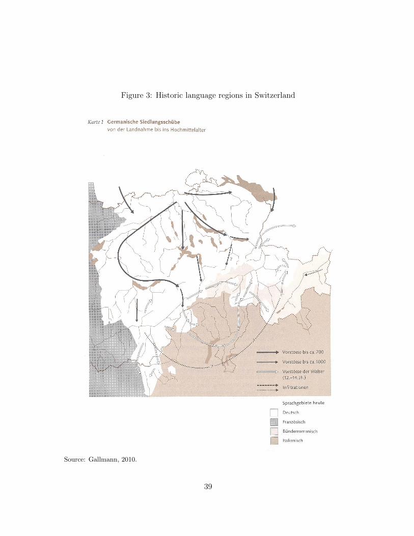
The geographical pattern of agglomeration of native speakers with differentlanguage background in Switzerland is strong and can best be visualized on a map ofthe country as in Figure 2. Each of the four colors corresponds to one language spokenby the majority (at least 50%) of inhabitants in a Swiss municipality.12 Of course,using a majoritarian rule to cut native language zones would be misleading if today’slanguage borders were largely different from the historical ones or the discontinuityabout language usage were rather smooth at the majority-based language borders.It turns out that historical and majority-rule-based language borders are the same(see Figure 3), and we will illustrate below that there is a clear (though not asharp) discontinuity about the main native language within relatively narrow spatialintervals around the Swiss internal historical language borders. We will utilize exactlythis discontinuity to infer the causal impact of language on measures of internationaltrade transactions of small spatial units.
– Figure 2 about here –
– as the second language, and the following six of the 21 (mostly) German-speaking cantons teachFrench as the second language: Bern, Basel-Landschaft, Basel Stadt, Fribourg, Solothurn, andValais. The other cantons teach English as the second language (Source: EDK Swiss Conferenceof Cantonal Ministers of Education).
11The deep cultural aspect particularly of native language was emphasized in anthropology (e.g.,the work of Franz Boas), linguistics (e.g., in Benjamin Whorf’s concept of linguistic relativity)and philosophy (e.g., the work of Johann Gottfried Herder, Wilhelm von Humboldt, or LudwigWittgenstein).
12While we use zip codes in the regression analysis, we employ municipality aggregates of zip codesin some of the graphical analysis for reasons of presentation.
7
It is worth emphasizing that language borders within Switzerland do not alwayscoincide with the ones of Cantons which have some economic and political autonomy(e.g., with regard to setting profit tax rates, etc.).13 As will become clear below, byisolating spatial units of different native language majority within cantons we maycondition on most economic, institutional, and political factors that may change atcantonal borders (certainly, in comparison to country-level studies; see also Brugger,Lalive, and Zweimuller, 2009; Eugster and Parchet, 2011).14
– Figure 3 about here –
The use of transaction-level data with spatial information is essential to ouranalysis for two reasons. First, it allows us to geo-spatially identify the locationof importers within Switzerland. This is essential to determine the majoritariannative language zone an importer resides in as well as her distance to the respectivelanguage border within Switzerland. Second, it reveals novel insights into theimpact of common native language on alternative margins of trade such as thenumber of bilateral transactions and the number of products traded as examples ofextensive margins, versus the value per transaction or the unit value as examplesof intensive margins. The latter may be useful to determine whether language ismainly a determinant of variable trade costs (as is commonly assumed; see Eggerand Lassmann, 2012) or of fixed trade costs.
The results in this study can be summarized as follows. Suppose we were interestedin the size of the discontinuity of the average of the three considered native languagesspoken in Switzerland at the intra-Swiss language borders. Then, we would have
13Politically, cantons can be compared to what are called States in the United States and Landerin Germany. The Swiss Federation consists of 26 cantons which joined the country sequentiallybetween 1291 (the foundation of inner Switzerland by the four German-speaking so-calledUrkantone) and 1815 (when the Congress of Vienna established independence of the SwissFederation and when the French-speaking cantons Geneve, Valais, and Neuchatel joined theFederation, consisting of 22 cantons by then). In 1979, the French-speaking canton Jura separatedfrom the canton of Berne and constituted the 26th canton (with six half-cantons that becamefull cantons as of the Constitution of 1999: Appenzell-Ausserrhoden, Appenzell-Innerrhoden,Basel-Stadt, Basel-Landschaft, Nidwalden, and Obwalden).
14In contrast to other studies exploiting language differences within Switzerland, we think of nativelanguage borders as to entail a fuzzy identification design. Most (but even not all) individualshave one native language. Yet, spatial aggregates host fractions of individuals of different nativelanguage. Hence, native language borders do not generate a sharp design: there are Germannative speakers on either side of the German-French border in Switzerland and the same is truefor French native speakers, etc. It has been neglected in earlier work that this calls for suitableidentification strategies (such as instrumental variable estimation) in order to render estimateddiscontinuities at language borders interpretable as (causal) local average treatment effects.
8
to consider the degree of fuzziness of native language: native German speakers onthe German-speaking versus the French-speaking (or Italian-speaking) side of thelanguage borders within Switzerland. If native language use jumped from zero (onthe untreated side) to one(-hundred percent; on the treated side) we would have asharp design. It turns out that this discontinuity is not one but about 0.66 (acrossall three native language usages and regions in Switzerland within a close enoughdistance around internal language borders). Hence, we could say that the degree offuzziness in the data amounts to about 34%. The estimated cultural bias on tradeinduced by common native language is estimated at 0.18 for import value and at0.20 for the number of import transactions. Hence, an increase in common nativelanguage similarity by 100 percent raises the import value share from countrieswith that native language by about 18 percentage points and that of the numberof import transactions by about 20 percentage points. We find significant positiveeffects on the share of import value, the number of transactions, and the number ofproducts imported from adjacent foreign countries with a (majoritarian) commonnative language as opposed to ones with a different native language. There is no sucheffect on the unit value, the value per transaction, or the quantity per transaction.Hence, common native language seems to affect bilateral trade primarily throughvarious extensive margins. Arguably, the latter points to common (at least native)language as a factor that reduces fixed market access costs rather than variable tradecosts. In addition, we provide evidence on the heterogeneity of the language effect.It turns out to differ with transaction size and across industries, and seems to bemore relevant for differentiated goods in comparison to homogeneous products.
The findings are important in three regards. First, they allow isolating andquantifying economic effects of pure cultural aspects of common native language. Apositive impact of common culture speaks to the relevance of the size of culturalcommunities and could tell an economic lesson against separatist movements thatdraw a romantic picture of cultural isolation that might ultimately lead to economicdisruption and a lack of economic prosperity. Second, a comparison of the findingswith naıve estimates in this paper and a large body of estimates in earlier worksuggests that aspects of language as a mere means of communication are probablynot much more important than cultural aspects (to some extent, this differs fromconclusions in Melitz and Toubal, 2012). However, the estimates nevertheless indicatethat there are also sizable potential gains from common spoken language, e.g., throughforeign language training in schools which can be affected by policy makers. Third,evidence of common language as a fixed trade cost factor may potentially influencethe specification of structural trade models which distinguish between fixed andvariable trade costs. For instance, modeling language effects on trade by way of fixedtrade costs may lead to largely different economic effects of common language in
9
general equilibrium relative to earlier research.
3 Common language as a driver of trade in the
literature
The interest in the role of language as a means of interaction and its consequencesfor outcome has its habitat at the interface of several disciplines within and at theboundaries of the social sciences.15 Common language – partly as a reflection ofcultural proximity – is understood to stimulate interaction in general and cross-bordertransactions of various kinds in particular.16
In the context of international economics, theoretical research identifies a rolefor common language as a mere means of communication or as a broader substrateon which common culture and externalities florish (see, e.g., Konya, 2006; Janeba,2007; and Melitz, 2012). Empirical research typically models common language as anon-tariff barrier to trade – mostly in the form of an iceberg-type, ad-valorem tradecost element among the numerous variable costs to trade. Among geographical andcultural trade-impeding or trade-facilitating factors (see McCallum, 1995; Helliwell,1996; Frankel and Romer, 1999; Eaton and Kortum, 2002; Anderson and van Wincoop,2004; Disdier and Head, 2008), common language is one of the usually employeddeterminants of trade costs usually employed in gravity models of bilateral goodstrade (see Helliwell, 1999; Melitz, 2008; Fidrmuc and Fidrmuc, 2009; Egger andLassmann, 2012; Melitz and Toubal, 2012; Sauter, 2012).
In a meta-analysis, Egger and Lassmann (2012) find that the language coefficientin gravity models likely captures confounding economic, cultural, and institutionaldeterminants in cross-country studies. In general, cultural proximity is viewed asan endogenous variable owing to confounding factors (see Disdier, and Mayer, 2007;Guiso, Sapienza, and Zingales, 2009; Felbermayr and Toubal, 2010). Accordingly, theparameter on common language indicators tends to be very sensitive to the exclusionof covariates among the determinants of bilateral trade flows – much more so than,e.g., that of bilateral distance (see Table 4 in Head and Mayer, 2013). Hence, thecommon language parameters in previous studies on the determinants of bilateral
15See Laitin (2000), Hauser, Chomsky, and Fitch (2002), Fidrmuc and Ginsburgh (2007), Holman,Schultze, Stauffer, and Wichmann (2007), Chiswick (2008), Fidrmuc and Fidrmuc (2009), Matser,van Oudenhoven, Askevis-Leherpeux, Florack, Hannover, and Rossier (2010), and Falck, Heblich,Lameli, and Sudekum (2012) for recent important contributions on the matter in political science,sociology, socio-linguistics, economics, and psychology.
16See the references to 81 studies in Egger and Lassmann (2012) for evidence on the language effecton international goods transactions.
10
trade should not be interpreted as to reflect a causal impact of common culture ontrade. Differentiating the communication and cultural aspects of common languageis difficult. Some authors have attempted measuring cultural proximity and avoidingthe bias of language coefficients through instrumental variables in a variety of relatedcontexts (e.g., Sauter, 2012 uses official language status across Canadian provincesas an instrument for spoken language in provinces). However, one would ideally usedata which allow for a better isolation of cultural from other aspects of language(see Falck, Heblich, Lameli, and Sudekum, 2012, for such an approach). The latter isa strategy pursued in this paper.
4 Transaction-level import data and spoken lan-
guages in Switzerland
4.1 Data sources
To identify the direct treatment effect of common native language for alternativemargins of bilateral imports, we use data from various sources. First of all, weutilize transaction-level import data (imports from abroad) of the Swiss FederalCustoms Administration (EDEC ) between January 2006 and June 2011. This datasource contains for the universe of import transactions (102,518,645 data points) thefollowing information (inter alia): an identifier for the importing authority (a person,a firm, or a political entity); an identifier of the address of the importing authority;the value per transaction; the quantity imported; the product (Harmonized System8-digit code; HS 8 ); the time (day and even hour) of entering the country; and thecountry of origin.17 We collapse this information at the zip code and country-of-originlanguage zone level across all years and compute the following outcome variables:the aggregate value of imports per country-of-origin language zone relative to allimports of that zip code for all dates and importing authorities covered, Valueshare; the number of transactions per country-of-origin language zone relative toall transactions of that zip code for all dates and importing authorities covered,Transactions share; the number of HS 8-digit product codes per country-of-originlanguage zone imported by that zip code for all dates and importing authoritiescovered, Number of products (HS8 tariff lines); the logarithm of the average unitvalue per country-of-origin language zone of all imports by that zip code for all dates
17Compared to the import data, the transaction-level export data at our disposal do not cover theuniverse of transactions (but only about 40%) so that we suppress the corresponding informationand results here and focus on imports.
11
and importing authorities covered, Log unit value; the logarithm of the value perimport transaction by country-of-origin language zone of all imports by that zip codefor all dates and importing authorities covered, Log value per transaction; and thelogarithm of the quantity per import transaction by country-of-origin language zoneof all imports by that zip code for all dates and importing authorities covered, Logquantity per transaction. The outcomes are based on trade with countries adjacentto Switzerland, with Germany and Austria as German-speaking exporters, France asthe French-speaking exporter and Italy as the Italian-speaking exporter.18
We match this information with geo-spatial data on the exact location of languageborders within Switzerland at 100-meter intervals. Language borders are determinedby exploiting zip-code-based information from the 1990 Census and GeographicalInformation Systems data of the Swiss Federal Statistical Office (Bundesamt furStatistik). Moreover, we utilize Geographical Information Systems data provided bySwisstopo (Amtliche Vermessung Schweiz) to determine the location of Swiss zipcode centroids in space and their Haversine distance in kilometers to all points alongthe internal language border in Switzerland as well as to all points along the nationalborder. This allows for an exact determination of the minimal great circle distanceof each zip code (of which there are 3,079 in the data) from the language border.19
The geospatial information and the use of distances to internal language borders iselemental for the identification strategy towards a causal effect of common nativelanguage as an aspect of common culture on trade. In particular, the chosen approachhelps avoiding a bias from omitted confounding factors. Moreover, we can utilize thegeospatial information to determine the minimal great circle distance of each spatialunit in Switzerland from the country’s external border (even of the external border
18Liechtenstein is a German-speaking country but, as indicated before, its trade flows are reportedwithin Switzerland’s trade statistics so that the country appears neither as a country of origin nor– due to its large distance to the Swiss language border – as an importing unit within Switzerland.
19These belong in 3,495 zip codes for the sample period of which 3,079 can be used after droppingRomansh, non-trading, and non-matchable (between customs and spatial data) zip codes. Unlikewith many firm-level data-sets available nowadays, the present one is untruncated. Hence, itcontains all transactions that cross Swiss international borders officially. Some transactionsare as small as one Swiss Franc. Moreover, since Switzerland charges a lower value-addedtax rate than its neighboring countries and most products from neighboring (European Unionmember) countries are exempted from tariffs, there is an incentive even for individuals to declareforeign-purchased products when entering Switzerland. More precisely, everything shipped intoSwitzerland by postal services is subject to customs checking (including taxation and, whereapplying, tariff payments). Personally imported goods of a value below 300 Swiss Francs can beimported without declaration, though one would save on taxes when declaring. For alcohol andother sensitive products, there are numerous exceptions from the 300 Swiss Francs rule, and evensmaller purchases have to be declared. More details on this matter are available from the authorsupon request.
12
of a specific foreign language zone). As alternative geo-spatial information, we usedata from Die Post to determine road distances from Swiss zip code centroids to theclosest point on the language border on a road. We conjecture that road distancesreflect transaction costs more accurately than great circle distances. In general, wefocus on spatial units within a radius of 50 kilometers from internal language interms of great circle or road distances with the zip code sample being generallysomewhat smaller for the latter than the former.20 The fact that the data containboth the intermediate importer and the final recipient as well as the shipper suggeststhat we are able to exploit all shipments imported by firms or individuals that arelocated within the zip codes included in our sample (we will assess the sensitivity ofthe results with regard to this point below).
Moreover, we augment the data-set by information on the mother tongue spokenin households per municipality from the 2000 Census. This information was kindlyprovided by the Swiss Federal Statistical Office (Bundesamt fur Statistik). Inconjunction with geo-spatial information, the data on the distribution of actualmother tongue may be used to measure the discontinuity in the majority use ofnative language as a percentage-point gap in mother tongue spoken of spatial unitson one side of the Swiss language border relative to exporting foreign language zonesto ones on the other side of the Swiss language border. Later on, this will allow usto express the estimated treatment effect of common language on various importaggregates per percentage point gap in common native language.
4.2 Descriptive statistics
The value of the average transaction in the covered sample is 9,930 Swiss Francs(CHF) and the median value is 376 CHF. Figures 4–7 summarize for all geographicalunits the frequency of positive import transactions per geographical unit withadjacent German-speaking, French-speaking, Italian-speaking, and (non-adjacent)other countries (rest of the world, RoW), respectively.
– Figures 4–7 about here –
The figures support the following conclusions. First, the share of positive importtransactions from the same language zone is generally higher for units with the samedominant mother tongue in Switzerland than for other regions. Very few spatial units
20Calculating minimal road distances of all zip codes to internal language borders in Switzerlandis time-consuming and costly. Since identification of the causal direct effect of common nativelanguage is local at the language border by way of the chosen design, it is unproblematic to focuson a band of 50 kilometers around internal language borders anyway.
13
outside the German- or Romansh-speaking parts have a similarly high concentrationof imports from Germany or Austria as the ones in those zones (see Figure 4). Thesame pattern is true for the French-speaking and the Italian-speaking parts of thecountry with respect to destinations that share a common language (see Figures5 and 6). Figure 7 shows that imports to the rest of the world are much moreevenly distributed over the three considered language regions. Unsurprisingly, ruralregions exhibit lower shares with the RoW than the densely populated regions inthe French-speaking part of the country and the Swiss-German agglomerations, inparticular around Zurich (the largest city of Switzerland) and Berne (the capital ofSwitzerland).21 Second, a randomly drawn unit from all over Switzerland accountsfor a larger share of import transactions from German-speaking countries than fromelsewhere for three reasons: the German-speaking part of Switzerland is relativelylarge, Germany is larger than France or Italy, and the transport network opennessof Switzerland to German-speaking countries is relatively higher than to otherlanguage zones due to (relevant, non-mountainous) border length, road accessibility,etc. Altogether, Figures 4–7 provide clear evidence of a language divide in theconcentration of import transactions in Switzerland.
– Tables 1–3 about here –
Tables 1–3 provide a more detailed overview of the importing behavior of Swissregions (zip codes) located within alternative (great circle) distance brackets fromthe language border.22 The tables indicate that Swiss regions import a larger shareof import volume or transactions and more products from neighboring countries witha common native language that is spoken by a majority of the inhabitants than onaverage. This pattern is similar for units within the same canton (see the lower panelof Tables 1–3) – where the language border within Switzerland divides a canton andinstitutional differences between treated and untreated regions are minimal – andfor all units (see the upper panel of Tables 1–3) at cross-cantonal or intra-cantonallanguage borders.23 Moreover, language differences appear to affect predominantly
21We will demonstrate later on that the pattern of RoW imports is non-discontinuous about internallanguage borders.
22The estimation procedures below will alternatively utilize road distances and great circle distancesto determine a zip code’s distance to the internal language border. For the sake of brevity (andsince results are very similar between the two concepts) and smaller sample size when using roaddistances at given distance bands to the internal language borders, we suppress numbers basedon road distance in Tables 1–3.
23Later on, we will provide evidence that average fixed importing zip code effects estimatedfrom a gravity model of log bilateral imports of Swiss zip codes from foreign countries are notdiscontinuous at the Swiss internal language borders. Hence, the differences in trade between
14
extensive transaction margins of trade (such as the share of transactions) but lessso intensive transaction margins of trade (such as the value per transaction or theunit value). Hence, the total value of a region’s imports is predominantly skewedtowards countries of origin with a common native language due to the number oftransactions and the number of products traded. This suggests that common nativelanguage mainly affects fixed transaction costs rather than marginal (or ad-valorem)trade costs, in contrast to traditional gravity modeling.
Let us just single out a few numbers for a discussion of Tables 1–3. According tothe bottom row of the top panel of Table 1, German-speaking regions in Switzerlandtrade on average 53.8% of their import volume and 51.9% of their transactions withGerman-speaking countries. These numbers are 50.9% and 47.1% for zip codeswhich are located on the German side of intra-cantonal Swiss language borders thatseparate French-speaking and German-speaking regions. They are 56.3% and 49%for German-speaking zip codes around the intra-cantonal language border betweenItalian-speaking and German-speaking regions. German-speaking Swiss regionsimport only 5.1% and 9.7% of their import volume from French- and Italian-speakingcountries of origin, respectively. The corresponding shares of transactions from thesesource countries are 3.6% and 8.6%, respectively. The same qualitative pattern (withsome quantitative differences) arises when considering French- and Italian-speakingregions’ common-language versus different-language imports.24 The same is truefor the number of imported products as shown in Table 2. Clearly, the number ofproducts imported from countries with a common native language spoken by themajority is relatively higher. On the other hand, Tables 2 and 3 do not confirm similarpatterns for the log unit value, the log value per transaction, and the log quantity pertransaction. These outcomes do not differ between imports from differing languagegroups. Tables 4–5 summarize further features of the Swiss spatially disaggregateddata.
– Tables 4–5 about here –
Table 4 indicates the number of zip codes in different language areas and distancebrackets from the Swiss internal language borders. For instance, that table demon-strates that the number of German-speaking regions in the data is much biggerthan that of French- and Italian-speaking regions. However, Table 4 suggests that
units with common and non-common language at internal language borders do not arise fromdifferences in characteristics which are specific to zip codes (such as income, taxation, or the like).
24The import shares of French-speaking regions from France tend to increase with increasingdistance from the respective language border, while import shares of Italian-speaking regionsfrom Italy tend to decrease with increasing distance from the language border.
15
the number of zip codes is relatively symmetric on either side of Swiss languageborders within symmetric distance bands around those borders. If all zip codes witha native majority of one of the three languages considered were used to infer theaverage treatment effect of common native language independent of their distanceto language borders, transactions from 3,079 zip codes could be utilized. Of those,only 986 zip codes would be used when focusing on intra-cantonal language borders.Of course, the number of zip codes used in estimation declines as one narrows thesymmetric distance window around language borders: there are 30 zip codes within a±1-kilometer band of language borders all over Switzerland of which 24 are located atintra-cantonal language borders; there are 706 zip codes within a ±20-kilometer bandof language borders all over Switzerland of which 435 are located at intra-cantonallanguage borders.
Table 5 indicates that the language border effect is drastic and discontinuousin the sense that, no matter how narrow of a distance band around the internalborder we consider, the one language is spoken by a large native majority while themajoritarian language of the adjacent different-language community accounts for apositive but much smaller fraction. Nevertheless, the design is fuzzy regarding theshare of individuals of any of the native languages considered on any side and type(French, German, Italian) of internal language border considered. This suggests thatthe parameter on majority-related common native language should not be interpretedas a local direct average treatment effect of common language (LATE; i.e., locally atthe language border). With a sharp design, the parameter would measure the LATEassociated with a jump of the difference in common native language from zero toone-hundred percent of all speakers.25
5 Spatial RDD estimation of the local average
treatment effect (LATE) of common native lan-
guage on trade
This section is organized in three subsections. First, we briefly outline the identifica-tion strategy of the LATE as a spatial regression discontinuity design in Subsection5.1. Then, we summarize the corresponding benchmark results regarding the LATEin Subsection 5.2. Finally, we assess the robustness of the findings and extensions invarious regards in Subsection 5.3.
25Melitz and Toubal (2012) provide evidence that the fraction of native language in virtually allexporting countries with only a single official language is less than 100%. Not surprisingly, this istrue as well for Switzerland.
16
5.1 A spatial regression discontinuity design (RDD) for theLATE of common native language majority
This paper’s empirical approach is based on the following identification strategy.Bilateral imports of geographical unit j = 1, ..., N which, in our case, is a Swiss zipcode, from country i are given by the relationship in Equation (1). Let us specify twosuch bilateral import relationships based on the latter equation. Imports of j from iare determined as Mij = eλCNLCNLijeλCSLCSLijdijµimjuij , where CNL and CSL reflectcommon native and common spoken language variables (shares), and ones of k fromi by Mik = eλCNLCNLikeλCSLCSLikdikµimkuik. Suppose that we pick countries and zipcodes such that CNLij ≥ 0.5 while CNLik < 0.5, CSLij ≈CSLik and dij ≈ dik. Then,
Mij
Mik
= eλCNLuijuik
(2)
Notice that λCNL can be estimated as a constant to the log-transformed relationshipin Equation (2), if (conditional or unconditional) independence of (CNLij − CNLik)and ln
uijuik
is achieved. Econometric theory proposes two elementary options toachieve such independence, instrumental variables estimation or – in very broadterms – a control function approach, where we subsume any form of controlling forobservable variables (with more or less flexible functional forms) under the latterapproach.26
The variable CNLij measures the share of speakers in zip code j with the samecommon native language as the majority of the population in exporting country i.Alternatively, we may determine a binary variable RULEij which is unity betweeni and j for, say, historically mainly German-speaking zip codes in Switzerland fortheir imports from Germany and Austria, and similarly for French-speaking andItalian-speaking zip codes with imports from France or Italy. Notice that we focusonly on imports from four included exporting countries which share common landborders with Switzerland (Austria, France, Germany, and Italy), for reasons of cleanidentification. As said before, the dominant language is the mother tongue of at least
26Hence, we use the term control function for conditioning on regressors beyond ones ineλCNLCNLijdij for all countries i and regions j in parametric and nonparametric frameworks.Naturally, this notion includes switching regression models, matching, as well as regression discon-tinuity designs (see Wooldridge, 2002), all of which may be portrayed as to involve some sort ofcontrol function (and some weighting of units). Notice that when formulating the control functionfor an outcome equation in terms of residuals from first-stage regressions, even instrumentalvariable estimation can be cast as a control function approach. In terms of the above notation,the usual approach adopted in the literature was one where the assumption was made that
E[uij
uik
]= 1, and all variables in the model were assumed to comprehensively control for dijµimj
for all units i, j, and k.
17
50% of the residents by definition, but not necessarily and even not actually of 100%.As indicated before and as is visible from Figures 8–10, treatment assignment isdiscontinuous but not sharp at the historical language borders, since the percentageof speakers is not 100% for any native language in any region.27 In addition, Figure11 – which is organized in such a way that the treatment (averaged within distancebins of 1 km) is shown in the vertical dimension, and panels on the left-hand side arebased on great circle distance to the language border as the forcing variable, whilepanels on the right-hand side are based on road distance to the language borderas the forcing variable – visualizes the discontinuity of treatment at the languageborder. Akin to Figures 8–10, it is shown that the discontinuity is pronounced butdoes not jump from zero to one at the border. The curvature is quite flat and similaron both sides of the language border.
– Figures 8–11 about here –
Let us generally refer to an import outcome of any kind for spatial unit j asyj. Recall from Section 4 that we employ six alternative bilateral import outcomes(generally referred to as yij) in the analysis: Value share; Transactions share; Numberof products (HS8 tariff lines); Log unit value; Log value per transaction; and Logquantity per transaction.
We follow the literature on regression discontinuity designs (RDDs; see Imbensand Lemieux, 2008; Angrist and Pischke, 2009; and Lee and Lemieux, 2010) andpostulate a flexible function about a so-called forcing variable, which may removethe endogeneity bias of the average treatment effect on outcome. For this, let usdefine the forcing variable for imports from country i by spatial unit (zip code) j, xij ,as the centered (road or great circle) distance to the intra-Swiss language border inkilometers. We code the forcing variable negatively in the non-treatment case (xij < 0if CNLij < 0.5)28 and positively in the treatment case (xij ≥ 0 if CNLij ≥ 0.5). Forconvenience, we will sometimes refer to zip codes with xij < 0 as to be situated to the
27The figures indicate that the share of the population speaking the native language spoken by themajority of the population in a zip code is higher than 80% in most regions, and that the changeat the language borders is drastic but not sharp. The degree of fuzziness may be measured by thedifference in the fraction of speakers of a common language to the ”right” of the border (in thetreatment region) and those to the ”left” of the border (in the control region). This differenceamounts to 0.66. This estimate is based on an optimally chosen bandwidth around internallanguage borders for treatment which amounts to 18 km (Imbens and Kalyanaraman, 2012). Anestimate across all three native language usages and regions in Switzerland within 50 km aroundinternal language borders amounts to 0.81. With a sharp design, the corresponding differencewould be unity. Hence, a larger deviation of that difference from unity is associated with a largerdegree of fuzziness.
28Then, there is a different language majority between j and the respective foreign language zone.
18
left of the border and ones with xij ≥ 0 as to be situated to the right of the border.Notice that the historical language borders which coincide with historical politicalborders probably do not appear randomly in space. However, this does not implythat a causal treatment effect of historical language borders cannot be identified (seeLee and Lemieux, 2010). The forcing variable in this paper is distance to languageborders. Observations are zip codes on either side of the border, and there is nodifference in the density or emergence of zip codes on either side of any languageborder in Switzerland. There is also no difference in the density or emergence ofindividual importers on either side of any language border in Switzerland, at leastnot when conditioning on intra-cantonal language borders. We will demonstratelater on that there is also no discontinuity about zip-code specific fixed effects aboutthe language borders that could confound the results.29
Let us define the sufficiently smooth (parametric polynomial or nonparametric)continuous functions f0(xij) at xij < 0, f1(xij) at xij ≥ 0, and f ∗1 (xij) ≡ f1(xij) −f0(xij). With a fuzzy treatment assignment design – where, say, any main languagezone in Switzerland contains native speakers of another main language type – as inthe data at hand, the average treatment effect (ATE) in an arbitrary geo-spatial unitand the local average treatment effect (LATE) in a close neighborhood to a Swissinternal language border of CNLij on outcome are defined as
ATE ≡ E[yij|xij ≥ 0]− E[yij|xij < 0]
E[CNLij|xij ≥ 0]− E[CNLij|xij < 0](3)
= λCNL + E
[f ∗1 (xij)
E[CNLij|xij ≥ 0]− E[CNLij|xij < 0]
]LATE ≡ lim
∆→0
(E[yij|0 ≤ xij < ∆]− E[yij| −∆ < xij < 0])
(E[CNLij|0 ≤ xij < ∆]− E[CNLij| −∆ < xij < 0])
= λCNL. (4)
Hence, ATE is the adjusted difference in conditional expectations of outcome betweentreated and untreated units, while LATE is the conditional expectation in outcomebetween treated and untreated units in the neighborhood of xij = 0. Both ATE andLATE are adjusted for the degree of fuzziness in the denominator which is a scalarin the open interval (0, 1) in case of some finite degree of fuzziness as is the case withthe data at hand. If treatment assignment is truly random conditional on xij andthere is no other discontinuity determining treatment assignment other than aboutxij. Then, the limit of the difference in conditional expectations in Equation (4) is
29Moreover, we discuss issues relating to placebo effects, measurement error, and other potentialproblems such as cross-border selling of importers, cross-border shopping of consumers, andcross-border working of natives of different languages in Section 5.3.
19
unconfounded by other covariates and there is no need to control for observablesbeyond f0(xij) and f1(xij).
30
Empirically, the adjustment through the denominator in (3) and (4) can easily
be made when regressing outcome yij on CNLij instead of CNLij (apart from the
control functions f0(.) and f1(.)), where CNLij is the prediction from a regression ofCNLij on the indicator variable RULEij which is unity whenever xij ≥ 0 and zeroelse (and on the control functions f0(.) and f1(.)).31
Regarding the design of the data-set for identification of the LATE of commonnative language on import outcomes, notice that each Swiss spatial unit (zip code)within a certain distance bracket to the left and the right of a Swiss language border isused up to thrice: once as a treated observation (xij ≥ 0) and up to twice (dependingon the considered distance window around language borders) as a control observation(xij < 0). This is because, say, a unit j in the German-speaking part and adjacent tothe French-speaking part of Switzerland is considered as treated with imports fromthe German-speaking foreign language zone but as untreated (control) with importsfrom the French-speaking or the Italian-speaking foreign language zone, respectively.Given the choice of a certain distance window around language borders, only unitswhich are within the respective window of two different language borders will showup thrice in the data.32
5.2 Main results
In the empirical analysis, we only consider zip codes within a radius of 50 kilometers(defined as either the minimum road or the minimum great circle distance) aroundinternal language borders in Switzerland. We summarize regression results for theLATE of a common native language of residents in a region on the aforementionedoutcomes for imports in Table 6 (using road distance as the forcing variable) and
30We will check this later on by additionally controlling for the demeaned distance of zip code jto the Swiss external language border to a specific language zone and by estimating LATE in asubsample of observations where λCNL is only estimated from units to the left and the right ofintra-cantonal language borders as is the case in the cantons of Bern (German/French), Valais(German/French), Fribourg (German/French), and Graubunden (German/Italian). Moreover, wewill demonstrate that, for a given exporting country i and bilateral imports of zip code j from iversus zip code k from i as in (1), there is no discontinuity about zip code-specific effects mj andmk at internal language borders in Switzerland.
31Of course, as is standard with two-stage least squares, the standard errors have to be adjusted
properly for the fact that CNLij is estimated rather than observed.32In the sample at hand, 15 German-speaking zip codes lie within 50 km from both the German-
French and the German-Italian language border if we use the great circle distance as a distancemeasure. The corresponding number with respect to road distance is 4.
20
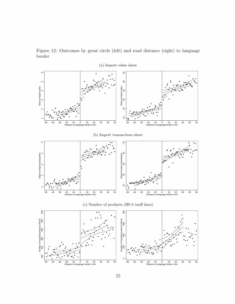
Table 7 (using great circle distance as the forcing variable) and in Figures 12 and 13.Notice that the adopted instrumental variable strategy entails that the estimatedparameter on common native language reflects the LATE associated with a jumpfrom zero (to the conceptual left of the border) to one-hundred percent (to theconceptual right of the border). Hence, the impact of common native languageper percentage point overlap in common native language amounts to 0.01× λCNL.Tables 6 and 7 contain eight numbered columns each, which indicate the functionalform of the control functions f0(xij) and f1(xij), and Figures 12 and 13 illustratethe estimates of the nonparametric control functions in Column (4) of Tables 6and 7. For each outcome considered, we report information with regard to thepoint estimate of LATE (λCNL) and its standard error with a parametric controlfunction and the correlation coefficient between the model prediction and the datawith a nonparametric control function, estimated in line with Fuji, Imbens, andKalyanaraman (2009) and Imbens and Kalyanaraman (2012). Moreover, we reportinformation on the number of cross-sectional units used for estimation, the R2, and –for nonparametric estimates – the chosen bandwidth.33 Tables 6 and 7 are organizedin four panels: the panel on the upper left contains the results for the LATE ofλCNL estimated from units within and across cantons; the panel on the upper rightestimates the LATE by conditioning not only on the control function based onthe forcing variables but also on the demeaned distance to Switzerland’s externalborder with the respective language;34 the two panels in the lower part of the tablescorrespond to the respective ones in the upper part but are only based on regressionsinvolving intra-cantonal language borders in Switzerland to eliminate institutionaldifferences between zip codes on two sides of a language border to the largest possibleextent.
– Tables 6–7 and Figures 12–13 about here –
The tables and figures suggest the following conclusions. First, the quantitativedifference between most of the comparable estimates of LATE on the same outcomein the upper left and upper right panels of Table 6 is relatively small and so is the onebetween the corresponding estimates of LATE in the upper and lower panels of Table6. Hence, the results suggest that the RDD about road distance to internal languageborders is capable of reducing substantially the possible bias of the LATE of common
33Recall that units may surface up to thrice in a regression: once as a treated and up to twice as acontrol unit. Therefore, the number of observations is relatively large in comparison to the onesreported in Table 4.
34Austria and Germany for German imports (relative to others), France for French imports, andItaly for Italian imports. The respective distance is demeaned properly such that λCNL stillmeasures the LATE of a common language majority.
21
language majorities on (Switzerland’s) import behavior. Second, model selectionamong the polynomial models based on the Akaike Information Criterion (AIC) assuggested by Lee and Lemieux (2010) leads to the choice of first-order to third-orderpolynomial control functions: higher-order polynomials are rejected in comparisondue to efficiency loss. The AIC is minimized for the first-order polynomial controlfunction for the value share and the transactions share. A second-order polynomialcontrol function is selected for the number of products as outcome and the logquantity per transaction. A third-order polynomial is selected for the log unit value.And a fifth-order polynomial is selected for the log value per transaction.35 Tables 6–7indicate that there is some sensitivity of the point estimates to the functional form ofthe control function. The reason for this might be that within a band of 50 kilometersaround the internal language borders the functional form of the control functionstill matters. Therefore, it may be preferable to consider a nonparametric ratherthan a parametric control function. The point estimates indicate that the first-orderpolynomial parametric control functions tend to generate LATE parameters whichtend to be closer to the nonparametric counterparts than the ones based on higher-order polynomials, on average. Third, utilizing the great circle distance instead ofroad distance in Table 7, the results are robust compared to Table 6. The LATEamounts to 0.222 for the import volume share, to 0.218 for the import transactionsshare and to 174 for the number of products with a parametric first-order polynomialcontrol function. With a nonparametric control function, it amounts to 0.179 withrespect to the import value share, to 0.199 regarding the import transaction share,and to 145 regarding the number of products. We find no significant effect regardingthe log unit value, the log value per transaction, and the log quantity per transaction.Finally, the results suggest that speaking a common native language mainly reducesfixed rather than variable trade costs. The latter flows from the fact that we identifyeffects mainly at extensive import margins in the upper part of each panel in thevertical dimension but not on intensive import margins.
Table 6 suggests a significant LATE of common native language of 0.187 forthe import volume share and 0.202 for the import transactions share, according toColumn (1) of Table 6. The LATE of common native language for the number oftransactions amounts to 186. Estimates based on a nonparametric control functionsuggest similar point estimates of the LATE in Column (4) of Table 6:36 0.179 forthe import volume share, 0.196 for the import transactions share, and 102 for the
35In general, also the Bayesian Information Criterion selects first-order to third-order controlfunctions. For the sake of brevity, we report LATEs involving either first-order to third-orderparametric control functions or nonparametric control functions in the tables.
36The bandwidth for the nonparametric estimator is determined by following Imbens and Kalya-naraman (2012). The selected bandwidths are always reported in the tables.
22
number of transactions. Hence, the import value share from a given country is about18 percentage points higher, the transaction share is almost 20 percentage pointshigher for a zip code with a common native language exporter than those sharesare for a comparable zip code with a different native language exporter. Regionsimport 142 additional products from a neighboring country sharing a commonnative language compared to different native language exporters. There is no robustevidence regarding effects of common native language on other considered tradeoutcomes. Akin to the parametric evidence, results based on the nonparametriccontrol function point to a dominance of effects of common native language on theextensive transaction margin of trade rather than at intensive margins (such as valueper transaction, quantity per transaction, or unit value).
Figures 12 and 13 visualize these results. While Figure 12 utilizes all zip codeswithin a certain distance to the language border in Switzerland, Figure 13 is only basedon zip codes to the right and the left of intra-cantonal language borders. Both figuresare organized in a similar way as Figure 11. They clearly suggest that discontinuitiesare more pronounced for extensive than intensive import transaction margins. Thefigures also suggest that the nonparametric control function eliminates the bias inthe treatment effect even within the full data sample (within ±50 kilometers fromthe internal language borders).
5.3 Sensitivity analysis and extensions
The results reported in Subsection 5.2 provided already some insights in the sensitivityof the LATE estimates of common native language (majority) on import behavior bycomparing results based on various (parametric and nonparametric) control functions,by considering road distance versus great circle distance as the forcing variable, andby comparing results for all zip codes within a certain window around the intra-Swisslanguage border versus ones that were located within the same canton. The aim ofthis section is to illustrate the qualitative insensitivity of the aforementioned resultsalong various lines and to provide further results based on components (in terms ofproduct and size categories) of imports rather than total imports.
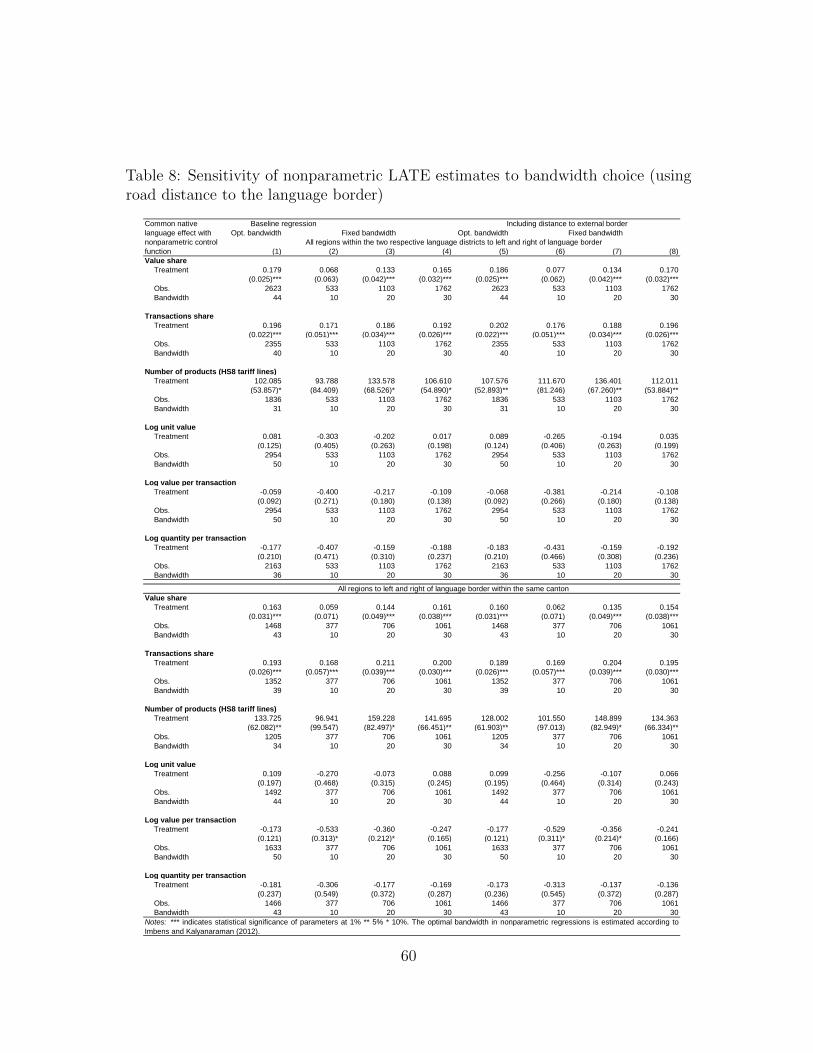
The nonparametric native language LATE for alternative bandwidthsIn a first step, we analyze the sensitivity of the nonparametric regressions to
different bandwidth choices in Table 8.
– Table 8 about here –
In Columns (1) and (5) of Table 8, we utilize the same bandwidths (see Imbensand Kalyanaraman, 2012) as in Columns (4) and (8) of Table 6. The remaining
23
nonparametric LATE estimates in Table 8 are based on fixed (lower than optimal)bandwidths in the other columns of Table 8.37 The corresponding findings suggestthat the results are fairly insensitive to choosing bandwidths between 20 and 30kilometers, and bandwidths at 10 kilometers produce insignificant LATE parameters.In general, bandwidths that are smaller than the optimal bandwidth lead to anefficiency loss, while bandwidths larger than the optimal one lead to larger bias.
Geographical placebo effects of the native language LATEMoreover, we undertake two types of placebo analysis to see whether disconti-
nuities of trade margins at internal language borders are spurious artifacts or not.For the first one, we consider the local average treatment effect of common nativelanguage on import outcomes from the rest of the world. The reason for this analysisis to check whether the pattern of trade around internal language borders indeedreflects a cultural relationship to the surrounding languages rather than spuriousdiscontinuities which could occur for other languages and cultural contexts as well.For this, we utilize a sharp RDD and define language to be unity for all Romanlanguages.
– Table 9 about here –
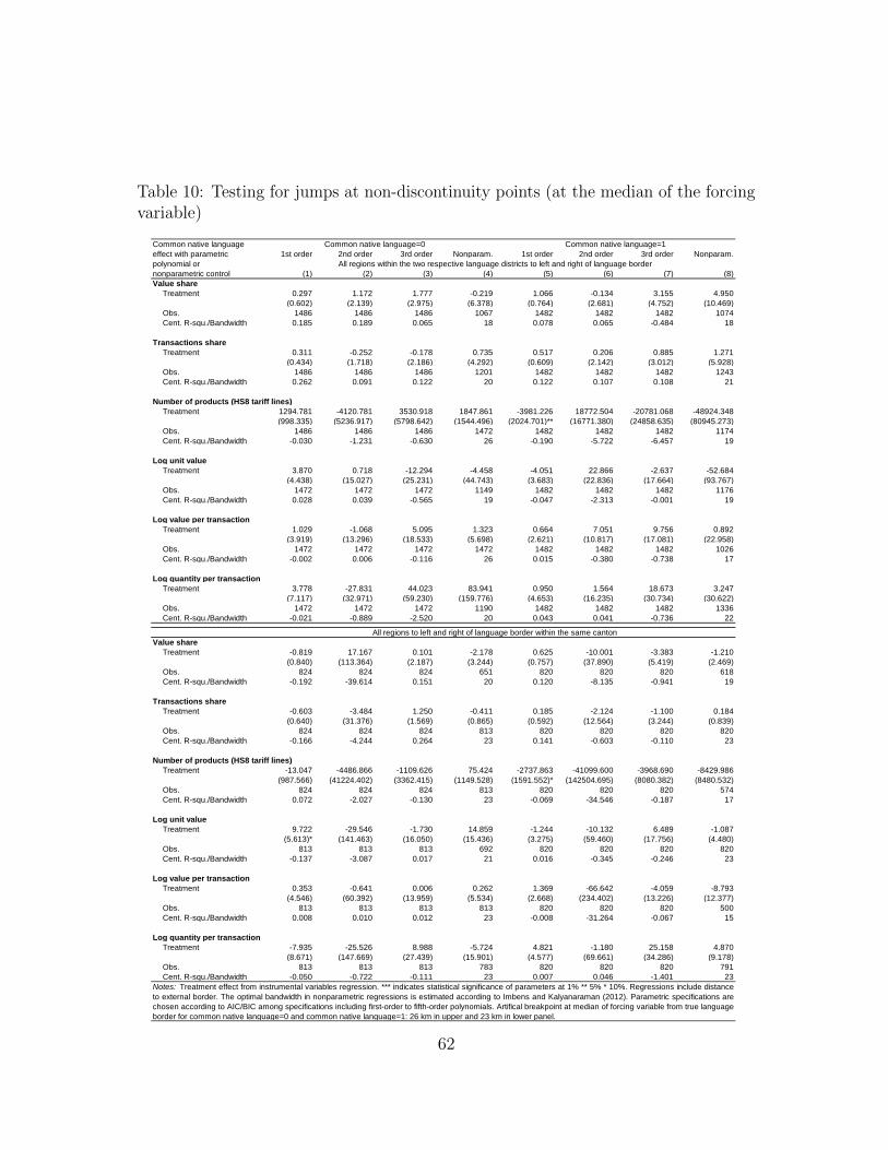
This analysis is summarized in Table 9, and it suggests that there is no systematiceffect of intra-Swiss language differences on imports from the rest of the world atthe internal language borders. For the second placebo analysis, we test whether weobserve discontinuities at points other than the majoritarian native language bordersby splitting the sample in subsamples with forcing variables of xij < 0 or xij > 0.Then, we test for discontinuities at the median level of the forcing variable in thosesubsamples. Table 10 suggests that such discontinuities do not appear at the median.
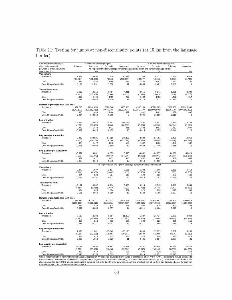
– Tables 10 and 11 about here –
Furthermore, Figures 12 and 13 suggest that a discontinuity might exist at adistance to the internal language border of about 15 kilometers. Table 11 provides anassessment of this issue. It turns out that a statistically significant discontinuity isonly detected with a first-order polynomial control function for import value shares
37The optimal bandwidth is about 40 kilometers for the extensive margins of interest, which isin line with bandwidths for outcomes chosen by the cross-validation criterion (these amount to37 km for the value and the transactions share, to 39 km for the number of products, to 49km for the log unit value, to 40 km for the log value per transaction, and to 50 km for the logquantity per transaction with all language borders). Since the cross-validation criterion suggestsa bandwidth below 10 km for treatment, we use fixed bandwidths of 10, 20 and 30 as alternatives.
24
with all (intra-cantonal and inter-cantonal internal border) data-points. Specificationswith parametric higher-order polynomial control functions or nonparametric controlfunctions do not identify a statistically significant discontinuity. Moreover, noneof the control function approaches detects a significant discontinuity at a placebolanguage border which is 15 kilometers away of the actual language border whenonly considering intra-cantonal placebo borders.
25
Lack of a RDD for fixed zip code-specific effects at internal languageborders
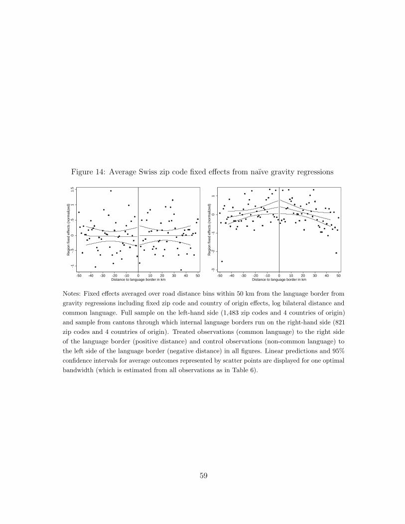
Since the underlying data are double-indexed (by Swiss zip code and foreigncountry), we may assess whether the importer-specific characteristics differ jointlybetween zip codes on the two sides of an internal language border. We illustrategraphically that zip code omitted variables are powerfully controlled for by the chosendesign in Figure 14. For this, we estimate gravity models of the form of equation(1). While the modeling of the trade cost function is quite standard across newtrade models, the structural interpretation of µi and mj depends on the underlyingtheoretical model.
– Figure 14 about here –
Figure 14 suggests that there is no discontinuity of zip code characteristics(regarding their size and consumer price index) at Swiss internal common nativelanguage borders. Hence, considering regional units close to the language borderswithin Switzerland powerfully eliminates important sources of heterogeneity acrossexporters and importers. Moreover, by the normalization of outcomes – i.e., usingimport value or transaction shares from the same language zone of origin, etc. – anypossible source of bias from a heterogeneity of foreign language zones is eliminatedanyway.
The native language LATE for alternative intensive product marginsHere, we consider three additional outcomes regarding intensive product (rather
than transaction) margins: log value per HS 8-digit product line; log unit value perproduct line; and log quantity per product line. The corresponding estimates aresummarized in Table 12.
– Table 12 about here –
Except for the log unit value per product, where the LATE amounts to 0.236with a nonparametric control function in Column (4) of Table 12, these intensiveproduct margins are not affected by common native language. Altogether, the resultsconfirm the earlier interpretation of the evidence about common (native) languageas a determinant of fixed rather than ad-valorem trade costs.
The native language LATE for specific internal language bordersNext, we assess the possibly varying magnitude of the LATE of interest for specific
internal language borders: the French-German and the German-Italian border withinSwitzerland. The corresponding results are summarized in Table 13. Columns (1)–(4)
26
refer to the French-German border and Columns (5)–(8) refer to the Italian-Germanborder.
– Table 13 about here –
We observe that the LATE is much higher for the latter, amounting to 0.285regarding the value share and to 0.293 regarding the transactions share, whenconsidering the nonparametric estimates in Column (8). It is 0.168 and 0.180,respectively, for the former sample in Column (4). Hence, common native language isnearly twice as important for the German-Italian border than for the French-Germanone. One explanation for this may be seen in the relative importance of geographicalbarriers (by way of the mountains)38 for the relative magnitude of cultural languagebarriers.
Beyond those border-specific results, we estimated the LATE for the internallanguage border in the canton of Fribourg only. The reason for this exercise was toeliminate any role of mountain barriers for the treatment effect of common nativelanguage. Doing so when using road distances to the internal border as the forcingvariable led to LATE estimates of 0.249 for the value share (with a standard errorof 0.067), and to 0.225 for the transactions share (with a standard error of 0.056)with a nonparametric control function. Hence, the corresponding results exhibit aslightly higher magnitude than the ones which are pooled across language treatmentsand language borders. Apart from that, the topographical barriers should not posemajor problems to our identification strategy in the sense that they would spuriouslyconfound the LATE of common native language. Transport routes such as tunnelsare nowadays well accessible (for instance, it takes only 20 minutes to cross theGotthardpass, which is the most important geographical barrier in the sample), andmost parts of the language border do not involve mountainous barriers anyway.
The native language LATE for specific native languagesBeyond differences in the native language LATE across language barriers, there
might be a difference with regard to specific native languages (or language treatments).One reason for this could be a greater general acceptance of or taste for goods from aspecific language zone across all customers. Notice that part of the effect in Table 13might be due to such heterogeneity already. Akin to the descriptive statistics aboutthe transactions share shown in Figures 4–6, we summarize the relative magnitudeof the LATE across the languages French, German, and Italian in Table 14.
– Table 14 about here –
38These alpine barriers are the Gotthardpass – a main transit route – and Berninapass.
27
In general, a distinction across the three native languages leads to a loss ofdegrees of freedom so that the LATE cannot be estimated at the same precision asthe pooled estimates. In any case, there is evidence of the LATE to be strongestfor imports from Italy when considering intra- and extra-cantonal language borderswithin Switzerland. With intra-cantonal language borders only the LATE for importsfrom France can be estimated at high-enough precision to reject the null hypothesis.The relative magnitude of the LATE for imports from France is comparable to thepooled estimates, irrespective of whether we consider all spatial units around internallanguage borders or only ones for intra-cantonal borders. The estimates for importsfrom Austria and Germany are somewhat smaller than the pooled ones, and theLATE estimates for imports from Italy are larger than the pooled estimates whenconsidering all spatial units at the top of Table 14.
The native language LATE in the size distribution of importersWith the analysis at stake, it is worthwhile to consider different effects of native
language on large versus small importers. The reason is that large importers might(i) more easily hire native workers from another language district (inducing workercommuting or migration) and (ii) engage in retailing. This would create fuzzinessabout the LATE.
– Table 15 about here –
To address this point in part, we augment the sensitivity analysis in Table 15by reporting results for each of the four quartiles of the distribution of respectiveoutcomes as used in Table 6. Since we consider road distance to be the preferableforcing variable, we base those results on road rather than great circle distance inthe control function. For the sake of brevity, we only report estimates including thedemeaned distance to respective national borders as a covariate. The nonparametricestimates in Table 15 suggest that the LATE is highest at the third quartile andlowest at the fourth quartile (of value shares and numbers of transactions).
Altogether, the findings in the previous subsection do not appear to be driven bylarge importers in particular. The quartile-specific results again point to the relevanceof common native language for fixed rather than ad-valorem trade costs. For thesmallest quartile of transaction sizes, the LATE is not only higher for extensivemargins of trade than in the highest quartile, but it is even positive and significantlydifferent from zero for log unit value and log value per transaction.
The native language LATE when excluding trading hubsThe effect of common native language may be biased by the fact that all zip
codes, including major trading hubs, are used. It may be interesting to exclude the
28
following zip codes in which customs offices that handle trade in goods accordingto the Swiss Federal Customs Administration are located: Aarau, Basel, Birsfelden,Bern, Brig-Glis, Chavornay, Le Noirmont, Mohlin, and Pratteln. These trading hubsnaturally coincide with the location of large warehouses and logistic centers. Whenexcluding the corresponding zip codes, the LATE amounts to 0.184 regarding thevalue share, to 0.200 regarding the transactions share, and to 171 regarding thenumber of products.39 These figures are similar to the ones reported in Table 6.
The native language LATE when accounting for cross-border shoppingOne would want to see how the LATE of common native language changes as
one excludes regional observations in the immediate proximity to the internal border.The latter would address the possibility of (internal language-)cross-border shoppingas a consumer side counterpart to the supplier side argument related to hiring ofnon-local-native language commuters. Again, commuting or cross-border shoppingwould induce measurement error about the LATE of common native language.
– Tables 16 – 18 about here –
To shed light on this matter, we leave out all observations within 5, 10, and15 kilometers around internal language borders and estimate the LATE from adiscontinuity at a distance of 10, 20, and 30 kilometer, respectively, in the forcingvariable in order to avoid measurement error in outcome by way of sales of goods atone side of the internal language border to customers at some distance on the otherside of the border. Compared to the nonparametric estimates in Table 6, Tables16 to 18 show that the nonparametric estimates of value and transactions sharesincrease to more than 0.2 if we leave out observations within 5, 10 and 15 kilometersfrom the language border. The estimates are robust across these three alternativetruncation choices.40 The pattern is the same – although less pronounced – for theparametric estimates.
The native language LATE for individual product categoriesFinally, there may be a genuine interest in the relative magnitude of the LATE
across alternative product categories for two reasons. First of all, preferences (and
39The corresponding estimates are based on a first-order polynomial specification, which is preferablewhen considering the AIC for the subsamples of data.
40The LATE for the value share amounts to 0.260, 0.262, and 0.270, respectively. It is 0.232, 0.242,and 0.276, respectively, for the transactions share. And it amounts to 128, 120, and 260 for thenumber of products, respectively. In addition, the LATE becomes significant if we leave outobservations within 5 and 10 kilometers for the log unit value.
29
the specific role of culture) might differ across products or product types and, second,the relative importance of variable and fixed trade costs might vary across products.
A first concern is that common culture by way of common native language mightbe more important for consumer goods than for intermediate goods. To shed light onthis, we singled out consumer goods according to the Swiss Federal Customs Officeto estimate the LATE of common native language only on those goods. The resultsare summarized in Table 19 for road distance as the forcing variable which suggeststhat there is no significant difference – neither qualitatively nor quantitatively – inthe sensitivity of all goods in Table 6 versus consumer goods only in Table 19 tocommon native language.
– Table 19 about here –
In Figure 15, we illustrate estimates of the LATE point estimates across allHS 2-digit product lines (of which there are 97) by way of kernel density plots,and in Table 20 we summarize the LATE estimates across three goods categories –homogeneous, reference-priced, and differentiated goods – according to the so-calledliberal classification by Rauch (1999). Both in Figure 15 and in Table 20 we utilizeroad distance as the forcing variable. The corresponding results may be summarizedas follows. Figure 15 suggests that the dispersion of the LATE is fairly high for alloutcomes. The LATE may be very high or even negative for some products, while the(by the industry share in terms of import value) weighted average is similar to thepoint estimates reported in Table 6. For instance, the LATE regarding the importvalue share is highest (amounting to 0.805) for Vegetable plaiting materials (HS 2-digitcode 14) and lowest (amounting to 0.203) for Electrical machinery and equipmentand parts, telecommunications equipment, sound recorders, television recorders (HS2-digit code 85). The LATE in the – in terms of import value and in descendingorder – most important 2-digit products in the data at hand – Jewelry (pearls, stones,precious metals, imitation jewelry, coins; HS 2-digit code 71), Machinery (nuclearreactors, boilers, machinery and mechanical appliances, computers; HS 2-digit code84), and Pharmaceutical products (HS 2-digit code 30) amounts to 0.282, 0.203, and0.419, respectively.
– Figure 15 and Table 20 about here –
Table 20 reveals that the impact of common native language is more pronouncedfor reference-priced and differentiated goods than for homogeneous goods. In partic-ular, there is a positive impact of common native language in those goods categoriesfor both reference-priced and differentiated good import value and transaction shares
30
and for differentiated good number of products. Even though we suppress the corre-sponding results here for the sake of brevity, similar conclusions could be drawn whenemploying the conservative classification by Rauch (1999). These results are broadlyin line with the findings in Melitz and Toubal (2012) who argue that cultural traitssuch as ethnic ties and trust are expected to be more important for differentiatedthan for homogeneous goods because trade in the former requires a larger amount ofinformation.41
To get a more precise image about the importance of CNL underlying thisrelatively broad goods classification, we accompany this analysis by some evidenceat the level of individual – HS 4-digit level– products based on their importancein terms of import volume. For this, let us consider one homogeneous productioninput (refined copper & alloys (no mast alloy), unwrought; HS 4-digit code 7403 )and one homogenous consumer good (fruit juices (& grape must) & veg. juice, nospirit; HS 4-digit code 2009 ).The LATE amounts to 0.802 regarding the value shareand to 0.751 regarding the transactions share for copper. It is 0.344 regarding thevalue share and 0.436 regarding the transactions share for fruit juice.42 Next, wepick two reference-priced goods (salt incl. table & dentrd., pure sodium chloride;HS 4-digit code 2501 ; and portland cement, aluminous cement, slag cement etc.; HS4-digit code 2523 ). The LATE is 0.528 regarding the value share and 0.661 regardingthe transactions share for salt. The respective figures amount to 0.540 and 0.497,and to 0.5 regarding the number of HS 8-digit product lines for cement.43 As analternative, we consider two differentiated consumer goods (women’s or girls’ suits,
41Notice that one could write Mij in (1) generically as
Mij = bijtijµimjuij , (5)
where bij would be some ij-specific Armington-type parameter in the spirit of Anderson (1979) orAnderson and van Wincoop (2004) and tij is a measure of (exponentiated) pure trade costs. If oneassumes in (1) that bij = 1 such that tij = eλlanguageijdij or tij = eλCNLCNLijeλCSLCSLijdij , alleffects of common language on bilateral imports are channeled through trade costs. In general, itcould be that bij = f(CNLij ,CSLij , dij) as well as tij = f(CNLij ,CSLij , dij). In the latter case,λCNL would measure the net impact of common native language of j from i through preferencesas well as trade costs. The evidence provided in this paper suggests that differentiated goodsdepend more strongly on common native language (i.e., common culture) than homogeneousgoods which provides some implicit support for a role of native language in preferences ratherthan only trade costs. However, it is not possible to discern the two channels quantitatively, sinceidentically indexed Armington and trade cost parameters exert an isomorphic impact on tradevolume.
42A first-order polynomial specification is chosen by the AIC for both products.43A first-order polynomial specification is chosen by the AIC for salt, and a third-order polynomial
specification is selected for cement.
31
ensemb. etc., not knit etc.; HS 4-digit code 6204 ; and motor cars & vehicles fortransporting persons; HS 4-digit code 8703 ). For suits, the LATE is 0.346 regardingthe value share, 0.339 regarding the transactions share, and 5 regarding the numberof products. The LATE is 0.249 for the value share, 0.311 for the transactionsshare, 1.5 for the number of products, and -0.841 for the log unit value for Cars.44
The choice of additional alternative products also provides significant results forLATE. Together with the results from Table 20, we conclude from this that nativelanguage barriers seem to relate more closely to fixed trade costs related to culturaldifferences. Although on average, the language effect seems to be more pronouncedfor reference-priced and differentiated goods than for homogenous goods, the analysisof individual products shows that the effect of common native language is overallimportant.
6 Conclusions
This paper combines three sources of information to isolate the impact of commonnative language as a measure of cultural proximity on international trade: geo-graphical information about language zones in Switzerland; transaction-level data oninternational trade by geographical site in Switzerland; and the distance of importersto internal language borders within Switzerland as well as to national borders. Thesedata let us infer the impact of common native language on international trade tolanguage zones corresponding to the ones around the internal language border inSwitzerland. The empirical framework chosen for such inference is a fuzzy regressiondiscontinuity design, focusing on import transaction data of three language zonesin Switzerland: German-speaking, French-speaking, and Italian-speaking. We con-sider different margins of trade of these zones from countries sharing a commonlanguage. We postulate flexible functional forms about the impact of distance-to-internal-language-border on such trade flows to identify the discontinuity of importingbehavior at the internal language borders. Since Swiss citizens quite proficientlyspeak the respective other (non-native) main languages of the country, especiallywithin regions in close proximity to internal language borders, we argue that thispaper is able to estimate the effect of common native language capturing commoncultural traits that generate common preferences, trust, and information about socialnorms of interaction, thereby leading to enhanced trade.
This strategy suggests effects of common native language of the following mag-nitude. The value share and the transactions share of a geographical unit from an
44A first-order polynomial specification is chosen for suits, and a second-order polynomial specifica-tion is selected for cars.
32
import destination are 18 and 20 percentage points higher, respectively, if commonnative language is the same. The effect is about 102 for the number of productsimported. We find no significant effect with respect to the unit value, the valueper transaction, and the quantity per transaction. We conclude that – by reducingfixed rather than variable trade costs – speaking a common native language mattersfor extensive margins rather than intensive margins of trade. In addition, the localaverage treatment effect differs among transaction size classes and substantiallyso across industries, where it seems to be more important for differentiated goodscategories rather than homogeneous products.
33
References
Anderson, James E., and Eric van Wincoop, 2003. Gravity with Gravitas: A Solution to theBorder Puzzle. American Economic Review 93 (1), 170–192.
Anderson, James E., and Eric van Wincoop, 2004. Trade Costs. Journal of Economic Literature42 (3), 691–751.
Angrist, Joshua, and Jorn-Steffen Pischke, 2009. Mostly Harmless Econometrics: An Empiricist’sCompanion. Princeton University Press: London.
Bossong, Georg, 2008. Die romanischen Sprachen. Eine vergleichende Einfuhrung. Helmut BuskeVerlag GmbH: Hamburg.
Brugger, Beatrix, Rafael Lalive, and Josef Zweimuller, 2009. Does Culture Affect Unemployment?Evidence from the Rostigraben. IZA Discussion Papers No. 4283, Institute for the Study ofLabor (IZA): Bonn.
Chiswick, Barry R., 2008. The Economics of Language: An Introduction and Overview. IZADiscussion Paper No. 3568, Institute for the Study of Labor (IZA): Bonn.
Casella, Alessandra, and James E. Rauch, 2002. Anonymous Market and Group Ties in Interna-tional Trade. Journal of International Economics 58 (1), 19–47.
Disdier, Anne-Celia, and Thierry Mayer, 2007. Je T’aime, Moi non Plus: Bilateral Opinions andInternational Trade. European Journal of Political Economy 23 (4), 1140–1159.
Disdier, Anne-Celia, and Keith Head, 2008. The Puzzling Persistence of the Distance Effect onBilateral Trade. The Review of Economics and Statistics 90 (1), 37–48.
Eaton, Jonathan, and Samuel Kortum, 2002. Technology, Geography, and Trade. Econometrica70 (5), 1741–1779.
Egger, Peter H., and Andrea Lassmann, 2012. The Language Effect in International Trade: AMeta-Analysis. Economics Letters 116 (2), 221–224.
Egger, Peter H., Mario Larch, Kevin Staub, and Rainer Winkelmann, 2011. The Trade Effects ofEndogenous Preferential Trade Agreements. American Economic Journal: Economic Policy3 (3), 113–143.
Eugster, Beatrix, and Raphael Parchet, 2011. Culture and Taxes: Towards Identifying Tax Com-petition. Cahiers de Recherches Economiques du Departement d’Econometrie et d’Economiepolitique (DEEP), Universite de Lausanne, Faculte des HEC, DEEP.
Falck, Oliver, Stephan Heblich, Alfred Lameli, and Jens Sudekum, 2012. Dialects, CulturalIdentity, and Economic Exchange. Journal of Urban Economics 72 (2), 225–239.
Felbermayr, Gabriel, and Farid Toubal, 2010. Cultural Proximity and Trade. European EconomicReview 54 (2), 279–293.
Fidrmuc, Jan, and Jarko Fidrmuc, 2009. Foreign Languages and Trade. CEPR Discussion Papers7228, C.E.P.R.: London.
Fidrmuc, Jan, and Victor Ginsburgh, 2007. Languages in the European Union: The Quest forEquality and Its Cost. European Economic Review 51 (6), 1351–1369.
34
Frankel, Jeffrey A., and David Romer, 1999. Does Trade Cause Growth? American EconomicReview 89 (3), 379–399.
Fuji, Daisuke, Guido W. Imbens, and Karthik Kalyanaraman, 2009. Notes for Matlab and StataRegression Discontinuity Software. Harvard University: Cambridge, MA.
Greif, Avner, 1989. Reputation and Coalitions in Medieval Trade: Evidence on the MaghribiTraders. Journal of Economic History 49 (4), 857–882.
Greif, Avner, 1993. Contract Enforceability and Economic Institutions in Early Trade: TheMaghribi Traders’ Coalition. American Economic Review 83 (3), 525–548.
Guiso, Luigi, Paola Sapienza, and Luigi Zingales, 2006. Does Culture Affect Economic Outcomes?Journal of Economic Perspectives 20 (2), 23–48.
Guiso, Luigi, Paola Sapienza, and Luigi Zingales, 2009. Cultural Biases in Economic Exchange?The Quarterly Journal of Economics 124 (3), 1095–1131.
Hauser, Marc D., Noam Chomsky, and W. Tecumseh Fitch, 2002. The Faculty of Language: WhatIs It, Who Has It, and How Did It Evolve? Science 22 298 (5598), 1569–1579.
Head, Keith, and Thierry Mayer, 2013. Gravity Equations: Workhorse, Toolkit, and Cookbook.CDEPR Discussion Paper no. 9322, C.E.P.R.: London.
Helliwell, John F., 1996. Do National Borders Matter for Quebec’s Trade? The Canadian Journalof Economics 29 (3), 507–522.
Helliwell, John F., 1999. Language and Trade. In: Breton, Albert (Ed.), Exploring the Economicsof Language. Canadian Heritage.
Helpman, Elhanan, and Paul R. Krugman, 1985. Market Structure and Foreign Trade. IncreasingReturns, Imperfect Competition and the International Economy. MIT Press: Cambridge,MA, and London.
Helpman, Elhanan, Marc Melitz, and Yona Rubinstein, 2008. Estimating Trade Flows: TradingPartners and Trading Volumes. The Quarterly Journal of Economics 123 (2), 441–487.
Holman, Eric, Christian Schultze, Dietrich Stauffer, and Søren Wichmann, 2007. On the Relationbetween Structural Diversity and Geographical Distance among Languages: Observationsand Computer Simulations. Linguistic Typology 11 (2), 393–422.
Imbens, Guido W., and Thomas Lemieux, 2008. Regression Discontinuity Designs: A Guide toPractice. Journal of Econometrics 142 (2), 615–635.
Imbens, Guido W., and Karthik Kalyanaraman, 2012. Optimal Bandwidth Choice for theRegression Discontinuity Estimator. Review of Economic Studies 79 (3), 933–959.
Janeba, Eckhard, 2007. International Trade and Consumption Network Externalities. EuropeanEconomic Review 51 (4), 781–803.
Konya, Istvan, 2006. Modeling Cultural Barriers in International Trade. Review of InternationalEconomics 14 (3), 494–507.
35
Krugman, Paul R., 1980. Scale Economies, Product Differentiation, and the Pattern of Trade.American Economic Review 70 (5), 950–959.
Laitin, David, 2000. What Is A Language Community? American Journal of Political Science 44(1), 142–155.
Lee, David S., and Thomas Lemieux, 2010. Regression Discontinuity Designs in Economics.Journal of Economic Literature 48 (2), 281–355.
Liver, Ricarda, 2010. Ratoromanisch: Eine Einfuhrung in das Bundnerromanische. 2nd edition,Narr Francke Attempto Verlag GmbH & Co. KG: Tubingen.
Lewis, M. Paul (ed.), 2009. Ethnologue: Languages of the World. 16th edition, SIL International:Dallas, TX. Online version: http://www.ethnologue.com/
Matser, Carine, Jan Pieter van Oudenhoven, Francoise Askevis-Leherpeux, Arnd Florack, BettinaHannover, and Jerome Rossier, 2010. Impact of Relative Size and Language on the Attitudesbetween Nations and Linguistic Groups: The Case of Switzerland. Applied Psychology: AnInternational Review 59 (1), 143–158.
Melitz, Marc J., 2003. The Impact of Trade on Intra-Industry Reallocations and AggregateIndustry Productivity. Econometrica 71 (6), 1695–1725.
Obstfeld, Maurice and Kenneth Rogoff, 2001. The Six Major Puzzles in International Macroe-conomics: Is There A Common Cause? NBER Macroeconomics Annual 2000, NBER:Cambridge, MA, 339–412.
Rauch, James E., 1999. Networks Versus Markets in International Trade. Journal of InternationalEconomics 48 (1), 7–35.
Rauch, James E., and Vitor Trindade, 2002. Ethnic Chinese Networks in International Trade.The Review of Economics and Statistics 84 (1), 116–130.
Sauter, Nikolas, 2012. Talking Trade: Language Barriers in Intra-Canadian Commerce. EmpiricalEconomics 42 (1), 301–323.
Wooldridge, Jeffrey M., 2002. Econometric Analysis of Cross Section and Panel Data. MIT Press:Cambridge, MA, and London.
36
Figure 1: Language regions in Switzerland and neighboring countries by nativelanguage majority
Data Source: Wikipedia; 1990 Census, Swiss Federal Statistical Office.
37
Figure 2: Language regions in Switzerland by native language majority
Data Source: 1990 Census, Swiss Federal Statistical Office. Thin lines represent municipality
borders, bold lines indicate cantonal and national borders. Official 50% majority cutoff. Those
borders are the same as the historical language borders associated with the political formation of
Switzerland.
38
Figure 3: Historic language regions in Switzerland
Source: Gallmann, 2010.
39
Figure 4: Share of transactions from German-speaking countries in total transactionsby zip code in %
Data source: Swiss Federal Customs Administration 2006–2011 and 1990 Census, Swiss Federal
Statistical Office. Bold red lines represent language borders, thin lines indicate zip code regions.
40
Figure 5: Share of transactions from France in total transactions by zip code in %
Data source: Swiss Federal Customs Administration 2006–2011 and 1990 Census, Swiss Federal
Statistical Office. Bold yellow lines represent language borders, thin lines indicate zip code regions.
41
Figure 6: Share of transactions from Italy in total transactions by zip code in %
Data source: Swiss Federal Customs Administration 2006–2011 and 1990 Census, Swiss Federal
Statistical Office. Bold purple lines represent language borders, thin lines indicate zip code regions.
42
Figure 7: Share of transactions from RoW in total transactions by zip code in %
Data source: Swiss Federal Customs Administration 2006–2011 and 1990 Census, Swiss Federal
Statistical Office. Bold red lines represent language borders, thin lines indicate zip code regions.
43
Tab
le1:
Des
crip
tive
stat
isti
csab
out
imp
orts
and
offici
alla
ngu
age
use
wit
hin
the
thre
em
ost
imp
orta
nt
langu
age
dis
tric
tsin
Sw
itze
rlan
d
0-1
80.7
45.2
10.5
40.0
6.8
62.8
43.6
13.2
34.6
13.5
1-2
85.2
37.8
9.4
35.8
7.2
81.4
35.2
17.9
31.9
15.7
2-5
94.6
42.4
7.3
43.4
5.1
87.0
30.2
28.2
26.9
23.8
5-10
97.5
51.9
6.2
49.2
4.6
90.5
31.1
26.4
29.4
21.6
10-2
097
.452
.36.
850
.74.
692
.929
.926
.126
.023
.320
-50
97.8
52.7
6.2
49.4
4.3
94.6
25.7
31.3
23.5
24.2
All
96.8
53.8
5.1
51.9
3.6
91.9
24.8
29.7
22.9
23.7
0-1
83.5
44.8
8.4
38.3
5.1
66.5
40.7
13.8
33.2
14.8
1-2
86.8
33.8
10.3
32.1
7.6
75.4
40.6
20.8
28.2
17.6
2-5
94.2
40.3
7.1
40.5
4.7
85.6
30.9
26.7
26.1
23.5
5-10
97.1
50.9
7.5
48.4
5.0
90.8
29.9
26.2
27.1
22.4
10-2
097
.652
.46.
949
.54.
893
.130
.024
.426
.722
.120
-50
98.2
53.0
6.5
48.3
4.1
96.1
25.8
27.5
22.3
22.9
All
96.9
50.9
6.9
47.1
4.5
91.5
29.2
25.5
25.3
22.1
0-1
--
--
-79
.04.
981
.69.
663
.91-
260
.730
.959
.023
.462
.471
.42.
683
.018
.658
.12-
591
.941
.942
.836
.135
.590
.425
.359
.315
.061
.15-
1091
.360
.428
.743
.825
.588
.024
.859
.119
.760
.310
-20
94.3
59.4
22.7
50.1
21.2
90.6
25.1
58.5
23.7
47.8
20-5
098
.257
.612
.652
.29.
986
.222
.458
.720
.950
.1A
ll96
.553
.89.
751
.98.
687
.319
.459
.818
.652
.2
0-1
--
--
-79
.04.
981
.69.
663
.91-
268
.537
.649
.425
.658
.671
.42.
683
.018
.658
.12-
589
.832
.751
.933
.243
.487
.340
.150
.415
.463
.55-
1089
.554
.934
.244
.328
.581
.916
.772
.214
.872
.710
-20
93.6
58.7
24.9
47.8
23.3
87.8
14.1
66.7
18.2
62.0
20-5
098
.057
.913
.851
.211
.388
.623
.561
.323
.554
.6A
ll95
.956
.319
.049
.016
.386
.120
.065
.219
.261
.4
All
regi
onal
uni
ts
Reg
iona
l uni
ts w
ithin
can
tons
thro
ugh
whi
ch in
trana
tiona
l FR
/DE
lang
uage
bor
der r
uns
% im
ports
from
Fr
ench
-spe
akin
g co
untri
es
All
regi
onal
uni
ts
Sw
iss
offic
ially
Ger
man
-spe
akin
g re
gion
sS
wis
s of
ficia
lly It
alia
n-sp
eaki
ng re
gion
s
Cha
ract
eris
tics
of re
gion
s at
the
Ger
man
-Ital
ian
lang
uage
bor
der w
ithin
Sw
itzer
land
Reg
iona
l uni
ts w
ithin
can
tons
thro
ugh
whi
ch in
trana
tiona
l IT/
DE
lang
uage
bor
der r
uns
Dis
tanc
e to
lang
uage
bo
rder
in k
ilom
eter
s%
Ger
man
sp
eake
rs
% im
ports
from
G
erm
an-s
peak
ing
coun
tries
% im
ports
from
Ita
lian-
spea
king
co
untri
es
% tr
ansa
ctio
ns fr
om
Ger
man
-spe
akin
g co
untri
es
% It
alia
n sp
eake
rs
% im
ports
from
Ita
lian-
spea
king
co
untri
es
% tr
ansa
ctio
ns fr
om
Ger
man
-spe
akin
g co
untri
es
% tr
ansa
ctio
ns fr
om
Italia
n-sp
eaki
ng
coun
tries
% tr
ansa
ctio
ns fr
om
Italia
n-sp
eaki
ng
coun
tries
% im
ports
from
G
erm
an-s
peak
ing
coun
tries
Cha
ract
eris
tics
of re
gion
s at
the
Ger
man
-Fre
nch
lang
uage
bor
der w
ithin
Sw
itzer
land
% tr
ansa
ctio
ns fr
om
Ger
man
-spe
akin
g co
untri
es
Dis
tanc
e to
lang
uage
bo
rder
in k
ilom
eter
s%
Ger
man
sp
eake
rs
% im
ports
from
G
erm
an-s
peak
ing
coun
tries
% tr
ansa
ctio
ns fr
om
Ger
man
-spe
akin
g co
untri
es
Sw
iss
offic
ially
Ger
man
-spe
akin
g re
gion
sS
wis
s of
ficia
lly F
renc
h-sp
eaki
ng re
gion
s
% tr
ansa
ctio
ns fr
om
Fren
ch-s
peak
ing
coun
tries
% tr
ansa
ctio
ns fr
om
Fren
ch-s
peak
ing
coun
tries
% F
renc
h sp
eake
rs
% im
ports
from
G
erm
an-s
peak
ing
coun
tries
% im
ports
from
Fr
ench
-spe
akin
g co
untri
es
Sourc
e:Sw
iss
Fed
eral
Cust
om
sA
dm
inis
trati
on
2006–2011
(ED
EC
).D
ista
nce
mea
sure
dby
gre
at
circ
ledis
tance
toth
ela
nguage
bor
der
.
44
Tab
le2:
Des
crip
tive
stat
isti
csab
out
trad
ean
doffi
cial
lan
guag
eu
sew
ith
inth
eth
ree
mos
tim
por
tant
lan
guag
edis
tric
tsin
Sw
itze
rlan
d(c
onti
nued
)
0-1
80.7
331
905.
35.
062
.822
311
25.
24.
51-
285
.250
816
05.
35.
781
.440
226
75.
25.
02-
594
.657
812
95.
45.
187
.028
321
45.
25.
35-
1097
.540
168
5.0
4.7
90.5
284
178
5.0
5.2
10-2
097
.452
389
5.1
4.6
92.9
205
170
5.3
5.2
20-5
097
.862
111
35.
04.
794
.622
820
65.
15.
0A
ll96
.866
010
75.
14.
891
.928
727
35.
35.
3
0-1
83.5
375
104
5.3
4.9
66.5
249
129
5.2
4.6
1-2
86.8
573
191
5.4
5.8
75.4
452
298
5.2
5.1
2-5
94.2
480
113
5.5
5.1
85.6
307
231
5.3
5.4
5-10
97.1
398
805.
04.
790
.827
618
15.
15.
210
-20
97.6
345
555.
04.
593
.118
614
95.
25.
020
-50
98.2
500
835.
14.
796
.121
019
45.
04.
8A
ll96
.945
984
5.1
4.7
91.5
230
183
5.1
5.0
0-1
--
--
-79
.027
116
4.5
4.9
1-2
60.7
3067
4.4
4.2
71.4
717
5.1
6.0
2-5
91.9
109
554.
73.
790
.471
171
5.0
3.5
5-10
91.3
210
141
5.1
4.0
88.0
8716
34.
64.
410
-20
94.3
214
204
4.8
3.8
90.6
8314
24.
64.
020
-50
98.2
345
845.
04.
486
.220
737
25.
14.
3A
ll96
.566
016
65.
14.
587
.320
442
05.
14.
4
0-1
--
--
-79
.027
116
4.5
4.9
1-2
68.5
3784
4.4
4.6
71.4
717
5.1
6.0
2-5
89.8
8258
4.5
3.2
87.3
7423
56.
73.
05-
1089
.523
616
85.
13.
981
.911
024
84.
94.
110
-20
93.6
233
226
4.9
3.9
87.8
6221
54.
53.
620
-50
98.0
248
704.
94.
488
.679
238
4.9
3.6
All
95.9
234
964.
94.
286
.178
225
4.9
3.8
All
regi
onal
uni
ts
Reg
iona
l uni
ts w
ithin
can
tons
thro
ugh
whi
ch in
trana
tiona
l IT/
DE
lang
uage
bor
der r
uns
# pr
oduc
ts (H
S 8
) fro
m G
erm
an-
spea
king
cou
ntrie
s
# pr
oduc
ts (H
S 8
) fro
m It
alia
n-sp
eaki
ng c
ount
ries
Log
unit
valu
e fro
m
Ger
man
-spe
akin
g co
untri
es
Log
unit
valu
e fro
m
Italia
n-sp
eaki
ng
coun
tries
Sw
iss
offic
ially
Ger
man
-spe
akin
g re
gion
sS
wis
s of
ficia
lly It
alia
n-sp
eaki
ng re
gion
s
Dis
tanc
e to
lang
uage
bo
rder
in k
ilom
eter
s%
Ger
man
sp
eake
rs
# pr
oduc
ts (H
S 8
) fro
m G
erm
an-
spea
king
cou
ntrie
s
# pr
oduc
ts (H
S 8
) fro
m It
alia
n-sp
eaki
ng c
ount
ries
Log
unit
valu
e fro
m
Ger
man
-spe
akin
g co
untri
es
Log
unit
valu
e fro
m
Italia
n-sp
eaki
ng
coun
tries
% It
alia
n sp
eake
rs
All
regi
onal
uni
ts
Reg
iona
l uni
ts w
ithin
can
tons
thro
ugh
whi
ch in
trana
tiona
l FR
/DE
lang
uage
bor
der r
uns
Cha
ract
eris
tics
of re
gion
s at
the
Ger
man
-Ital
ian
lang
uage
bor
der w
ithin
Sw
itzer
land
% F
renc
h sp
eake
rs
# pr
oduc
ts (H
S 8
) fro
m G
erm
an-
spea
king
cou
ntrie
s
# pr
oduc
ts (H
S 8
) fro
m F
renc
h-sp
eaki
ng c
ount
ries
Log
unit
valu
e fro
m
Ger
man
-spe
akin
g co
untri
es
Cha
ract
eris
tics
of re
gion
s at
the
Ger
man
-Fre
nch
lang
uage
bor
der w
ithin
Sw
itzer
land
Sw
iss
offic
ially
Ger
man
-spe
akin
g re
gion
sS
wis
s of
ficia
lly F
renc
h-sp
eaki
ng re
gion
s
Dis
tanc
e to
lang
uage
bo
rder
in k
ilom
eter
s%
Ger
man
sp
eake
rs
# pr
oduc
ts (H
S 8
) fro
m G
erm
an-
spea
king
cou
ntrie
s
# pr
oduc
ts (H
S 8
) fro
m F
renc
h-sp
eaki
ng c
ount
ries
Log
unit
valu
e fro
m
Ger
man
-spe
akin
g co
untri
es
Log
unit
valu
e fro
m
Fren
ch-s
peak
ing
coun
tries
Log
unit
valu
e fro
m
Fren
ch-s
peak
ing
coun
tries
Sourc
e:Sw
iss
Fed
eral
Cust
om
sA
dm
inis
trati
on
2006–2011
(ED
EC
).D
ista
nce
mea
sure
dby
gre
at
circ
ledis
tance
toth
ela
nguage
bor
der
.
45
Tab
le3:
Des
crip
tive
stat
isti
csab
out
trad
ean
doffi
cial
lan
guag
eu
sew
ith
inth
eth
ree
mos
tim
por
tant
lan
guag
edis
tric
tsin
Sw
itze
rlan
d(c
onti
nued
)
0-1
80.7
8.2
8.4
6.3
7.0
62.8
8.3
8.2
6.7
6.5
1-2
85.2
8.0
8.2
6.2
6.5
81.4
8.3
8.4
6.7
7.3
2-5
94.6
8.4
8.5
6.8
6.8
87.0
8.3
8.4
6.9
6.8
5-10
97.5
8.3
8.2
6.7
6.7
90.5
8.3
8.4
6.7
6.8
10-2
097
.48.
28.
36.
76.
992
.98.
28.
26.
66.
920
-50
97.8
8.3
8.3
6.8
7.0
94.6
8.2
8.4
6.5
7.3
All
96.8
8.4
8.3
6.9
6.6
91.9
8.2
8.4
6.5
7.1
0-1
83.5
8.2
8.4
6.4
6.6
66.5
8.4
8.2
6.7
6.5
1-2
86.8
8.1
8.2
6.1
6.0
75.4
8.4
8.1
6.8
7.0
2-5
94.2
8.2
8.4
6.5
6.5
85.6
8.4
8.4
7.0
6.9
5-10
97.1
8.3
8.4
6.7
7.1
90.8
8.4
8.4
6.8
6.8
10-2
097
.68.
28.
26.
66.
993
.18.
18.
26.
66.
820
-50
98.2
8.2
8.1
6.6
6.8
96.1
8.1
8.2
6.5
7.1
All
96.9
8.2
8.2
6.6
6.8
91.5
8.2
8.2
6.6
6.9
0-1
--
--
-79
.07.
48.
35.
77.
81-
260
.78.
57.
75.
47.
671
.45.
07.
40.
24.
22-
591
.97.
98.
36.
28.
390
.48.
78.
46.
47.
85-
1091
.38.
67.
96.
78.
688
.08.
38.
26.
37.
110
-20
94.3
8.1
7.9
6.6
7.6
90.6
7.9
8.4
6.0
7.6
20-5
098
.28.
27.
96.
78.
086
.28.
18.
36.
17.
2A
ll96
.58.
48.
16.
96.
087
.38.
08.
36.
07.
4
0-1
--
--
-79
.07.
48.
35.
77.
81-
268
.58.
87.
65.
75.
771
.45.
07.
40.
24.
22-
589
.87.
68.
36.
08.
187
.39.
98.
07.
57.
45-
1089
.58.
58.
56.
57.
781
.98.
38.
26.
47.
010
-20
93.6
8.1
7.7
6.7
6.0
87.8
7.9
8.3
6.4
7.6
20-5
098
.08.
17.
96.
65.
988
.67.
78.
15.
47.
6A
ll95
.98.
17.
96.
66.
186
.18.
08.
15.
97.
4
Log
quan
tity/
trans
actio
n fro
m F
renc
h-sp
eaki
ng c
ount
ries
Cha
ract
eris
tics
of re
gion
s at
the
Ger
man
-Fre
nch
lang
uage
bor
der w
ithin
Sw
itzer
land
Sw
iss
offic
ially
Ger
man
-spe
akin
g re
gion
sS
wis
s of
ficia
lly F
renc
h-sp
eaki
ng re
gion
s
Dis
tanc
e to
lang
uage
bo
rder
in k
ilom
eter
s%
Ger
man
sp
eake
rs
Log
valu
e/tra
nsac
tion
from
Ger
man
-sp
eaki
ng c
ount
ries
Log
valu
e/tra
nsac
tion
from
Fre
nch-
spea
king
cou
ntrie
s
% F
renc
h sp
eake
rs
Log
valu
e/tra
nsac
tion
from
Ger
man
-sp
eaki
ng c
ount
ries
Log
valu
e/tra
nsac
tion
from
Ital
ian-
spea
king
co
untri
es
% It
alia
n sp
eake
rs
All
regi
onal
uni
ts
Reg
iona
l uni
ts w
ithin
can
tons
thro
ugh
whi
ch in
trana
tiona
l FR
/DE
lang
uage
bor
der r
uns
Cha
ract
eris
tics
of re
gion
s at
the
Ger
man
-Ital
ian
lang
uage
bor
der w
ithin
Sw
itzer
land
% G
erm
an
spea
kers
Log
quan
tity/
trans
actio
n fro
m G
erm
an-
spea
king
cou
ntrie
s
Log
quan
tity/
trans
actio
n fro
m It
alia
n-sp
eaki
ng
coun
tries
All
regi
onal
uni
ts
Reg
iona
l uni
ts w
ithin
can
tons
thro
ugh
whi
ch in
trana
tiona
l IT/
DE
lang
uage
bor
der r
uns
Log
valu
e/tra
nsac
tion
from
Ger
man
-sp
eaki
ng c
ount
ries
Log
quan
tity/
trans
actio
n fro
m It
alia
n-sp
eaki
ng
coun
tries
Sw
iss
offic
ially
Ger
man
-spe
akin
g re
gion
sS
wis
s of
ficia
lly It
alia
n-sp
eaki
ng re
gion
s
Dis
tanc
e to
lang
uage
bo
rder
in k
ilom
eter
s
Log
valu
e/tra
nsac
tion
from
Ger
man
-sp
eaki
ng c
ount
ries
Log
valu
e/tra
nsac
tion
from
Fre
nch-
spea
king
cou
ntrie
s
Log
quan
tity/
trans
actio
n fro
m G
erm
an-
spea
king
cou
ntrie
s
Log
quan
tity/
trans
actio
n fro
m G
erm
an-
spea
king
cou
ntrie
s
Log
quan
tity/
trans
actio
n fro
m F
renc
h-sp
eaki
ng c
ount
ries
Log
valu
e/tra
nsac
tion
from
Ital
ian-
spea
king
co
untri
es
Log
quan
tity/
trans
actio
n fro
m G
erm
an-
spea
king
cou
ntrie
s
Sourc
e:Sw
iss
Fed
eral
Cust
om
sA
dm
inis
trati
on
2006–2011
(ED
EC
).D
ista
nce
mea
sure
dby
gre
at
circ
ledis
tance
toth
ela
nguage
bor
der
.
46
Tab
le4:
Num
ber
ofzi
pco
de
regi
ons
indiff
eren
tla
ngu
age
dis
tric
tsan
din
vari
ous
dis
tance
inte
rval
sar
ound
inte
rnal
Sw
iss
langu
age
bor
der
s
Num
ber o
f zip
cod
es in
Fre
nch-
Ger
man
par
tFr
ench
Ger
man
Num
ber o
f zip
cod
es in
Ger
man
-Ital
ian
part
Ger
man
Italia
nU
niqu
e su
m
With
in 1
km o
f FR
/DE
intra
natio
nal b
orde
r14
15W
ithin
1km
of D
E/IT
intra
natio
nal b
orde
r0
130
With
in 5
km o
f FR
/DE
intra
natio
nal b
orde
r70
81W
ithin
5km
of D
E/IT
intra
natio
nal b
orde
r13
1017
4W
ithin
10k
m o
f FR
/DE
intra
natio
nal b
orde
r13
116
0W
ithin
10k
m o
f DE/
IT in
trana
tiona
l bor
der
2529
345
With
in 2
0km
of F
R/D
E in
trana
tiona
l bor
der
268
318
With
in 2
0km
of D
E/IT
intra
natio
nal b
orde
r50
7070
6W
ithin
50k
m o
f FR
/DE
intra
natio
nal b
orde
r54
373
9W
ithin
50k
m o
f DE/
IT in
trana
tiona
l bor
der
235
198
1700
All
808
1993
All
1993
278
3079
With
in 1
km o
f FR
/DE
intra
natio
nal b
orde
r12
11W
ithin
1km
of D
E/IT
intra
natio
nal b
orde
r0
124
With
in 5
km o
f FR
/DE
intra
natio
nal b
orde
r48
62W
ithin
5km
of D
E/IT
intra
natio
nal b
orde
r10
512
5W
ithin
10k
m o
f FR
/DE
intra
natio
nal b
orde
r84
112
With
in 1
0km
of D
E/IT
intra
natio
nal b
orde
r20
1322
9W
ithin
20k
m o
f FR
/DE
intra
natio
nal b
orde
r17
120
0W
ithin
20k
m o
f DE/
IT in
trana
tiona
l bor
der
4222
435
With
in 5
0km
of F
R/D
E in
trana
tiona
l bor
der
281
475
With
in 5
0km
of D
E/IT
intra
natio
nal b
orde
r15
236
929
Thro
ugh
whi
ch in
trana
tiona
l FR
/DE
lang
uage
bor
der r
uns
281
517
Thro
ugh
whi
ch in
trana
tiona
l DE/
IT la
ngua
ge b
orde
r run
s15
137
986
With
in 1
km o
f FR
/DE
intra
natio
nal b
orde
r16
18W
ithin
1km
of D
E/IT
intra
natio
nal b
orde
r4
543
With
in 5
km o
f FR
/DE
intra
natio
nal b
orde
r61
59W
ithin
5km
of D
E/IT
intra
natio
nal b
orde
r11
1214
3W
ithin
10k
m o
f FR
/DE
intra
natio
nal b
orde
r10
912
1W
ithin
10k
m o
f DE/
IT in
trana
tiona
l bor
der
1918
267
With
in 2
0km
of F
R/D
E in
trana
tiona
l bor
der
232
259
With
in 2
0km
of D
E/IT
intra
natio
nal b
orde
r30
3255
3W
ithin
50k
m o
f FR
/DE
intra
natio
nal b
orde
r56
172
6W
ithin
50k
m o
f DE/
IT in
trana
tiona
l bor
der
120
7914
82Al
l80
819
93Al
l19
9327
830
79W
ithin
1km
of F
R/D
E in
trana
tiona
l bor
der
1416
With
in 1
km o
f DE/
IT in
trana
tiona
l bor
der
43
37W
ithin
5km
of F
R/D
E in
trana
tiona
l bor
der
4350
With
in 5
km o
f DE/
IT in
trana
tiona
l bor
der
108
111
With
in 1
0km
of F
R/D
E in
trana
tiona
l bor
der
6994
With
in 1
0km
of D
E/IT
intra
natio
nal b
orde
r16
1018
9W
ithin
20k
m o
f FR
/DE
intra
natio
nal b
orde
r14
416
9W
ithin
20k
m o
f DE/
IT in
trana
tiona
l bor
der
2516
354
With
in 5
0km
of F
R/D
E in
trana
tiona
l bor
der
258
434
With
in 5
0km
of D
E/IT
intra
natio
nal b
orde
r10
131
820
Thro
ugh
whi
ch in
trana
tiona
l FR
/DE
lang
uage
bor
der r
uns
281
517
Thro
ugh
whi
ch in
trana
tiona
l DE/
IT la
ngua
ge b
orde
r run
s15
137
986
Offi
cial
lang
uage
Offi
cial
lang
uage
Usi
ng ro
ad d
ista
nces
Usi
ng g
reat
circ
le d
ista
nces
Sou
rce:
1990
Cen
sus,
Sw
iss
Fed
eral
Sta
tist
ical
Offi
ce.
Dis
tan
cem
easu
red
by
gre
at
circ
led
ista
nce
toth
ela
ngu
age
bord
er.
47
Tab
le5:
Pop
ula
tion
shar
esac
cord
ing
tola
ngu
age
inva
riou
sdis
tance
inte
rval
sar
ound
inte
rnal
Sw
iss
langu
age
bor
der
sin
%
DE
regi
ons
FR re
gion
sD
E re
gion
sFR
regi
ons
DE
regi
ons
IT re
gion
sD
E re
gion
sIT
regi
ons
With
in 1
km o
f lan
guag
e bo
rder
80.7
36.1
18.4
62.8
-21
.0-
79.0
With
in 5
km o
f lan
guag
e bo
rder
89.5
17.9
9.2
80.6
82.3
11.9
16.9
87.4
With
in 1
0km
of l
angu
age
bord
er93
.413
.25.
585
.286
.611
.512
.687
.8W
ithin
20k
m o
f lan
guag
e bo
rder
95.4
9.5
3.5
89.2
90.4
9.5
8.8
89.4
With
in 5
0km
of l
angu
age
bord
er96
.86.
92.
091
.996
.511
.22.
987
.3Al
l96
.86.
92.
091
.996
.511
.22.
987
.3W
ithin
1km
of l
angu
age
bord
er83
.532
.215
.666
.5-
21.0
-79
.0W
ithin
5km
of l
angu
age
bord
er90
.219
.88.
778
.783
.417
.615
.882
.4W
ithin
10k
m o
f lan
guag
e bo
rder
93.3
14.5
5.8
83.9
86.5
17.5
12.6
82.1
With
in 2
0km
of l
angu
age
bord
er95
.210
.14.
088
.690
.214
.99.
084
.4W
ithin
50k
m o
f lan
guag
e bo
rder
96.9
7.4
2.2
91.5
95.9
13.1
3.5
86.1
Thro
ugh
whi
ch la
ngua
ge b
orde
r run
s96
.97.
42.
291
.595
.913
.13.
586
.1
Dis
tanc
e bi
ns fr
om la
ngua
ge b
orde
r
Ger
man
-Fre
nch
spea
king
lang
uage
bor
der r
egio
nsG
erm
an-It
alia
n sp
eaki
ng la
ngua
ge b
orde
r reg
ions
Ger
man
spe
aker
sFr
ench
spe
aker
sG
erm
an s
peak
ers
Italia
n sp
eake
rs
Sou
rce:
2000
Cen
sus,
Sw
iss
Fed
eral
Sta
tist
ical
Offi
ce.
Dis
tan
cem
easu
red
by
gre
at
circ
led
ista
nce
toth
ela
ngu
age
bord
er.
48
Figure 8: Share of German-speaking population and language borders in Switzerland
lines indicate cantonal and national borders and purple lines indicate language borders according to
the official 50% rule. The figure shows the share of Italian-speaking population in German, French,
and Italian speaking population.
51
Figure 11: Treatment probability by great circle (left) and road distance (right) tolanguage border
(a) All cantons
0.2
.4.6
.81
Sha
re o
f lan
guag
e po
pula
tion
-50 -40 -30 -20 -10 0 10 20 30 40 50Distance to language border in km
0.2
.4.6
.81
Sha
re o
f lan
guag
e po
pula
tion
-50 -40 -30 -20 -10 0 10 20 30 40 50Distance to language border in km
(b) Cantons through which internal language borders run
0.2
.4.6
.81
Sha
re o
f lan
guag
e po
pula
tion
-50 -40 -30 -20 -10 0 10 20 30 40 50Distance to language border in km
0.2
.4.6
.81
Sha
re o
f lan
guag
e po
pula
tion
-50 -40 -30 -20 -10 0 10 20 30 40 50Distance to language border in km
Notes: Treated observations (common language) to the right side of the language border (positive
distance) and control observations (non-common language) to the left side of the language border
(negative distance) in all figures.
52
Table 6: LATE estimates of the impact of common language on imports from commonlanguage speaking bordering countries to Switzerland (using road distance to thelanguage border)
1st order 2nd order 3rd order Nonparam. 1st order 2nd order 3rd order Nonparam.
Notes: Treatment effect from instrumental variables regression. *** indicates statistical significance of parameters at 1% ** 5% * 10%. The optimal bandwidth innonparametric regressions is estimated according to Imbens and Kalyanaraman (2012). Parametric specifications are chosen according to AIC/BIC amongspecifications including first-order to fifth-order polynomials.
All regions to left and right of language border within the same canton
Common native language effect with parametric polynomial or nonparametric control function
Baseline regression Including distance to external border
All regions within the two respective language districts to left and right of language border
53
Table 7: LATE estimates of the impact of common language on imports from commonlanguage speaking bordering countries to Switzerland (using great-circle distance tothe language border)
1st order 2nd order 3rd order Nonparam. 1st order 2nd order 3rd order Nonparam.
Notes: Treatment effect from instrumental variables regression. *** indicates statistical significance of parameters at 1% ** 5% * 10%. The optimal bandwidth innonparametric regressions is estimated according to Imbens and Kalyanaraman (2012). Parametric specifications are chosen according to AIC/BIC amongspecifications including first-order to fifth-order polynomials.
All regions to left and right of language border within the same canton
Common native language effect with parametric polynomial or nonparametric control function
Baseline regression Including distance to external border
All regional units within the two respective language districts to left and right of language border
54
Figure 12: Outcomes by great circle (left) and road distance (right) to languageborder
(a) Import value share
.1.2
.3.4
.5.6
Sha
re o
f im
port
val
ue
-50 -40 -30 -20 -10 0 10 20 30 40 50Distance to language border in km
1020
3040
5060
Sha
re o
f im
port
val
ue-50 -40 -30 -20 -10 0 10 20 30 40 50
Distance to language border in km
(b) Import transactions share
.1.2
.3.4
.5S
hare
of i
mpo
rt tr
ansa
ctio
ns
-50 -40 -30 -20 -10 0 10 20 30 40 50Distance to language border in km
1020
3040
50S
hare
of i
mpo
rt tr
ansa
ctio
ns
-50 -40 -30 -20 -10 0 10 20 30 40 50Distance to language border in km
(c) Number of products (HS 8 tariff lines)
100
200
300
400
500
600
Num
ber
of im
port
ed p
rodu
cts
(HS
8)
-50 -40 -30 -20 -10 0 10 20 30 40 50Distance to language border in km
020
040
060
080
0N
umbe
r of
impo
rted
pro
duct
s (H
S 8
)
-50 -40 -30 -20 -10 0 10 20 30 40 50Distance to language border in km
55
Figure 12: (continued)
(d) Log unit value
4.5
55.
5Lo
g im
port
uni
t val
ue
-50 -40 -30 -20 -10 0 10 20 30 40 50Distance to language border in km
44.
55
5.5
Log
impo
rt u
nit v
alue
-50 -40 -30 -20 -10 0 10 20 30 40 50Distance to language border in km
(e) Log value per transaction
7.6
7.8
88.
28.
48.
6Lo
g in
tens
ive
mar
gin
of im
port
s
-50 -40 -30 -20 -10 0 10 20 30 40 50Distance to language border in km
7.8
88.
28.
48.
68.
8Lo
g in
tens
ive
mar
gin
of im
port
s
-50 -40 -30 -20 -10 0 10 20 30 40 50Distance to language border in km
(f) Log quantity per transaction
66.
57
7.5
8Lo
g im
port
qua
ntity
per
tran
sact
ion
-50 -40 -30 -20 -10 0 10 20 30 40 50Distance to language border in km
66.
57
7.5
8Lo
g im
port
qua
ntity
per
tran
sact
ion
-50 -40 -30 -20 -10 0 10 20 30 40 50Distance to language border in km
Notes: Treated observations (common language) to the right side of the language border (positive
distance) and control observations (non-common language) to the left side of the language border
(negative distance) in all figures. Linear predictions and 95% confidence intervals for average
outcomes represented by scatter points are displayed for one optimal bandwidth (which is estimated
from all observations).56
Figure 13: Outcomes by great circle (left) and road distance (right) to languageborder in cantons through which internal language borders run
(a) Import value share
.1.2
.3.4
.5.6
Sha
re o
f im
port
val
ue
-50 -40 -30 -20 -10 0 10 20 30 40 50Distance to language border in km
020
4060
Sha
re o
f im
port
val
ue-50 -40 -30 -20 -10 0 10 20 30 40 50
Distance to language border in km
(b) Import transactions share
.1.2
.3.4
.5S
hare
of i
mpo
rt tr
ansa
ctio
ns
-50 -40 -30 -20 -10 0 10 20 30 40 50Distance to language border in km
010
2030
4050
Sha
re o
f im
port
tran
sact
ions
-50 -40 -30 -20 -10 0 10 20 30 40 50Distance to language border in km
(c) Number of products (HS 8 tariff lines)
020
040
060
080
0N
umbe
r of
impo
rted
pro
duct
s (H
S 8
)
-50 -40 -30 -20 -10 0 10 20 30 40 50Distance to language border in km
020
040
060
080
0N
umbe
r of
impo
rted
pro
duct
s (H
S 8
)
-50 -40 -30 -20 -10 0 10 20 30 40 50Distance to language border in km
57
Figure 13: (continued)
(d) Log unit value
44.
55
5.5
6Lo
g im
port
uni
t val
ue
-50 -40 -30 -20 -10 0 10 20 30 40 50Distance to language border in km
44.
55
5.5
Log
impo
rt u
nit v
alue
-50 -40 -30 -20 -10 0 10 20 30 40 50Distance to language border in km
(e) Log value per transaction
77.
58
8.5
9Lo
g in
tens
ive
mar
gin
of im
port
s
-50 -40 -30 -20 -10 0 10 20 30 40 50Distance to language border in km
77.
58
8.5
9Lo
g in
tens
ive
mar
gin
of im
port
s
-50 -40 -30 -20 -10 0 10 20 30 40 50Distance to language border in km
(f) Log quantity per transaction
55.
56
6.5
77.
5Lo
g im
port
qua
ntity
per
tran
sact
ion
-50 -40 -30 -20 -10 0 10 20 30 40 50Distance to language border in km
56
78
Log
impo
rt q
uant
ity p
er tr
ansa
ctio
n
-50 -40 -30 -20 -10 0 10 20 30 40 50Distance to language border in km
Notes: Treated observations (common language) to the right side of the language border (positive
distance) and control observations (non-common language) to the left side of the language border
(negative distance) in all figures. Linear predictions and 95% confidence intervals for average
outcomes represented by scatter points are displayed for one optimal bandwidth (which is estimated
from all observations).58
Figure 14: Average Swiss zip code fixed effects from naıve gravity regressions
-1-.
50
.51
1.5
Reg
ion
fixed
effe
cts
(nor
mal
ized
)
-50 -40 -30 -20 -10 0 10 20 30 40 50Distance to language border in km
-3-2
-10
1R
egio
n fix
ed e
ffect
s (n
orm
aliz
ed)
-50 -40 -30 -20 -10 0 10 20 30 40 50Distance to language border in km
Notes: Fixed effects averaged over road distance bins within 50 km from the language border from
gravity regressions including fixed zip code and country of origin effects, log bilateral distance and
common language. Full sample on the left-hand side (1,483 zip codes and 4 countries of origin)
and sample from cantons through which internal language borders run on the right-hand side (821
zip codes and 4 countries of origin). Treated observations (common language) to the right side
of the language border (positive distance) and control observations (non-common language) to
the left side of the language border (negative distance) in all figures. Linear predictions and 95%
confidence intervals for average outcomes represented by scatter points are displayed for one optimal
bandwidth (which is estimated from all observations as in Table 6).
59
Table 8: Sensitivity of nonparametric LATE estimates to bandwidth choice (usingroad distance to the language border)
Notes: *** indicates statistical significance of parameters at 1% ** 5% * 10%. The optimal bandwidth in nonparametric regressions is estimated according toImbens and Kalyanaraman (2012).
All regions to left and right of language border within the same canton
Common native language effect with nonparametric control function
Baseline regression Including distance to external border
All regions within the two respective language districts to left and right of language borderFixed bandwidthFixed bandwidth
60
Table 9: Sharp parametric LATE estimates of the impact of common languageon imports from the rest of the world to Switzerland (using road distance to thelanguage border)
1st order 2nd order 3rd order Nonparam. 1st order 2nd order 3rd order Nonparam.
Notes: Treatment effect from OLS regression. *** indicates statistical significance of parameters at 1% ** 5% * 10%. Regressions without distance to external border. Theoptimal bandwidth in nonparametric regressions is estimated according to Imbens and Kalyanaraman (2012). Parametric specifications are chosen according to AIC/BIC amongspecifications including first-order to fifth-order polynomials.
Sharp treatment effect with parametric polynomial or nonparametric control function
Treatment=Roman language
All regions within the two respective language districts to left and right of language border
All regions to left and right of language border within the same canton
61
Table 10: Testing for jumps at non-discontinuity points (at the median of the forcingvariable)
1st order 2nd order 3rd order Nonparam. 1st order 2nd order 3rd order Nonparam.
Notes: Treatment effect from instrumental variables regression. *** indicates statistical significance of parameters at 1% ** 5% * 10%. Regressions include distanceto external border. The optimal bandwidth in nonparametric regressions is estimated according to Imbens and Kalyanaraman (2012). Parametric specifications arechosen according to AIC/BIC among specifications including first-order to fifth-order polynomials. Artifical breakpoint at median of forcing variable from true languageborder for common native language=0 and common native language=1: 26 km in upper and 23 km in lower panel.
Common native language effect with parametric polynomial or nonparametric control
Common native language=0 Common native language=1
All regions within the two respective language districts to left and right of language border
All regions to left and right of language border within the same canton
62
Table 11: Testing for jumps at non-discontinuity points (at 15 km from the languageborder)
1st order 2nd order 3rd order Nonparam. 1st order 2nd order 3rd order Nonparam.
Notes: Treatment effect from instrumental variables regression. *** indicates statistical significance of parameters at 1% ** 5% * 10%. Regressions include distance toexternal border. The optimal bandwidth in nonparametric regressions is estimated according to Imbens and Kalyanaraman (2012). Parametric specifications arechosen according to AIC/BIC among specifications including first-order to fifth-order polynomials. Artifical breakpoint at 15 km from true language border for commonnative language=0 and common native language=1.
Common native language effect with parametric polynomial or nonparametric control function
Common native language=0 Common native language=1
All regions within the two respective language districts to left and right of language border
All regions to left and right of language border within the same canton
63
Tab
le12
:L
AT
Ees
tim
ates
ofth
eim
pac
tof
com
mon
langu
age
onim
por
tsfr
omco
mm
onla
ngu
age
spea
kin
gb
order
ing
countr
ies
toSw
itze
rlan
d(u
sing
road
dis
tance
toth
ela
ngu
age
bor
der
)on
pro
duct
inte
nsi
vem
argi
ns
1st o
rder
2nd
orde
r3r
d or
der
Non
para
m.
1st o
rder
2nd
orde
r3r
d or
der
Non
para
m.
(1)
(2)
(3)
(4)
(5)
(6)
(7)
(8)
Log
valu
e pe
r pro
duct
(HS8
tarif
f lin
es)
Trea
tmen
t0.
004
-0.0
44-0
.076
-0.0
19-0
.018
-0.0
54-0
.078
-0.0
34(0
.062
)(0
.103
)(0
.144
)(0
.075
)(0
.061
)(0
.100
)(0
.141
)(0
.075
)O
bs.
2954
2954
2954
2783
2954
2954
2954
2783
Cen
t. R
-squ
./Ban
dwid
th0.
001
0.00
30.
004
470.
046
0.04
80.
048
47
Log
unit
valu
e pe
r pro
duct
Trea
tmen
t0.
130
0.27
80.
239
0.23
60.
140
0.29
40.
256
0.25
2(0
.066
)**
(0.1
08)*
*(0
.152
)(0
.098
)**
(0.0
65)*
*(0
.107
)***
(0.1
51)*
(0.0
99)*
*O
bs.
2954
2954
2954
2044
2954
2954
2954
2044
Cen
t. R
-squ
./Ban
dwid
th0.
009
0.01
40.
014
340.
029
0.03
30.
033
34
Log
quan
tity
per p
rodu
ctTr
eatm
ent
-0.0
89-0
.292
-0.2
97-0
.237
-0.1
22-0
.315
-0.3
12-0
.262
(0.1
00)
(0.1
65)*
(0.2
32)
(0.1
44)
(0.0
97)
(0.1
61)*
(0.2
27)
(0.1
43)*
Obs
. 29
5429
5429
5420
5229
5429
5429
5420
52C
ent.
R-s
qu./B
andw
idth
0.00
30.
008
0.00
835
0.04
90.
054
0.05
535
Log
valu
e pe
r pro
duct
(HS8
tarif
f lin
es)
Trea
tmen
t-0
.046
-0.0
76-0
.117
-0.0
56-0
.063
-0.0
49-0
.083
-0.0
58(0
.080
)(0
.126
)(0
.170
)(0
.087
)(0
.079
)(0
.124
)(0
.167
)(0
.085
)O
bs.
1633
1633
1633
1633
1633
1633
1633
1633
Cen
t. R
-squ
./Ban
dwid
th0.
004
0.00
60.
008
500.
038
0.03
90.
040
50
Log
unit
valu
e pe
r pro
duct
Trea
tmen
t0.
177
0.38
40.
306
0.30
00.
183
0.35
40.
273
0.28
0(0
.088
)**
(0.1
37)*
**(0
.184
)*(0
.131
)**
(0.0
86)*
*(0
.135
)***
(0.1
82)
(0.1
28)*
*O
bs.
1633
1633
1633
1063
1633
1633
1633
1063
Cen
t. R
-squ
./Ban
dwid
th0.
022
0.03
00.
030
300.
049
0.05
50.
055
30
Log
quan
tity
per p
rodu
ctTr
eatm
ent
-0.1
88-0
.418
-0.3
76-0
.340
-0.2
12-0
.364
-0.3
10-0
.304
(0.1
33)
(0.2
08)*
*(0
.280
)(0
.177
)*(0
.129
)(0
.203
)*(0
.275
)(0
.171
)*O
bs.
1633
1633
1633
1138
1633
1633
1633
1138
Cen
t. R
-squ
./Ban
dwid
th0.
008
0.01
50.
016
330.
052
0.05
60.
057
33N
otes
:Tr
eatm
ent
effe
ctfro
min
stru
men
talv
aria
bles
regr
essi
on.
***
indi
cate
sst
atis
tical
sign
ifica
nce
ofpa
ram
eter
sat
1%**
5%*
10%
.Th
eop
timal
band
wid
thin
nonp
aram
etric
regr
essi
ons
ises
timat
edac
cord
ing
toIm
bens
and
Kal
yana
ram
an(2
012)
.P
aram
etric
spec
ifica
tions
are
chos
enac
cord
ing
toA
IC/B
ICam
ong
spec
ifica
tions
incl
udin
g fir
st-o
rder
to fi
fth-o
rder
pol
ynom
ials
.
All
regi
ons
to le
ft an
d rig
ht o
f lan
guag
e bo
rder
with
in th
e sa
me
cant
on
Com
mon
nat
ive
lang
uage
ef
fect
with
par
amet
ric
poly
nom
ial o
r non
para
met
ric
cont
rol f
unct
ion
Bas
elin
e re
gres
sion
Incl
udin
g di
stan
ce to
ext
erna
l bor
der
All
regi
ons
with
in th
e tw
o re
spec
tive
lang
uage
dis
trict
s to
left
and
right
of l
angu
age
bord
er
64
Table 13: LATE estimates of the impact of common language on imports fromcommon language speaking bordering countries to Switzerland by language borderregion (using road distance to the language border)
1st order 2nd order 3rd order Nonparam. 1st order 2nd order 3rd order Nonparam.
Notes: Treatment effect from instrumental variables regression. *** indicates statistical significance of parameters at 1% ** 5% * 10%. Regressions include distance toexternal border. The optimal bandwidth in nonparametric regressions is estimated according to Imbens and Kalyanaraman (2012). Parametric specifications arechosen according to AIC/BIC among specifications including first-order to fifth-order polynomials.
Common native language effect with parametric polynomial or nonparametric control function
French-German speaking regions only Italian-German speaking regions only
All regions within the two respective language districts to left and right of language border
All regions to left and right of language border within the same canton
65
Table 14: LATE estimates of the impact of common language on imports fromcommon language speaking bordering countries to Switzerland for specific nativelanguages (using road distance to the language border)
1st order 2nd order 3rd order Nonparam. 1st order 2nd order 3rd order Nonparam. 1st order 2nd order 3rd order Nonparam.
Notes: Treatment effect from instrumental variables regression. Non-common native language speaking regions to the left and common native language speaking regions to the right side of the language border. *** indicates statisticalsignificance of parameters at 1% ** 5% * 10%. The optimal bandwidth in nonparametric regressions is estimated according to Imbens and Kalyanaraman (2012). Parametric specifications are chosen according to AIC/BIC amongspecifications including first-order to fifth-order polynomials.
Imports from Austria and Germany
All regions within the two respective language districts to left and right of language border
All regions to left and right of language border within the same canton
Common native language effect with parametric polynomial or nonparametric control function
Imports from France Imports from Italy
66
Tab
le15
:L
AT
Ees
tim
ates
ofth
eim
pac
tof
com
mon
langu
age
onim
por
tsfr
omco
mm
onla
ngu
age
spea
kin
gb
order
ing
countr
ies
toSw
itze
rlan
din
diff
eren
tquar
tile
sof
the
dis
trib
uti
onof
the
dep
enden
tva
riab
les
(usi
ng
road
dis
tance
toth
ela
ngu
age
bor
der
)
1st o
rder
2nd
orde
r3r
d or
der
Non
para
m.
1st o
rder
2nd
orde
r3r
d or
der
Non
para
m.
1st o
rder
2nd
orde
r3r
d or
der
Non
para
m.
1st o
rder
2nd
orde
r3r
d or
der
Non
para
m.
(1)
(2)
(3)
(4)
(5)
(6)
(7)
(8)
(9)
(10)
(11)
(12)
(13)
(14)
(15)
(16)
Valu
e sh
are
Trea
tmen
t0.
332
0.31
10.
261
0.30
80.
315
0.31
00.
278
0.29
50.
366
0.33
80.
315
0.34
30.
289
0.25
70.
174
0.26
0(0
.021
)***
(0.0
35)*
**(0
.050
)***
(0.0
30)*
**(0
.021
)***
(0.0
36)*
**(0
.051
)***
(0.0
31)*
**(0
.021
)***
(0.0
35)*
**(0
.049
)***
(0.0
33)*
**(0
.022
)***
(0.0
37)*
**(0
.053
)***
(0.0
33)*
**O
bs.
2880
2880
2880
2212
2897
2897
2897
2332
2889
2889
2889
2183
2904
2904
2904
2251
Cen
t. R
-squ
./Ban
dwid
th0.
533
0.53
30.
530
400.
520
0.52
10.
519
420.
529
0.52
80.
527
400.
456
0.45
50.
451
41
Tran
sact
ions
sha
reTr
eatm
ent
0.32
90.
297
0.25
00.
299
0.31
30.
296
0.25
50.
285
0.36
20.
335
0.31
10.
339
0.31
50.
276
0.22
60.
282
(0.0
19)*
**(0
.032
)***
(0.0
46)*
**(0
.029
)***
(0.0
21)*
**(0
.036
)***
(0.0
51)*
**(0
.031
)***
(0.0
21)*
**(0
.035
)***
(0.0
49)*
**(0
.033
)***
(0.0
20)*
**(0
.034
)***
(0.0
48)*
**(0
.033
)***
Obs
. 28
8028
8028
8021
4828
9728
9728
9723
2828
8928
8928
8922
0429
0429
0429
0420
31C
ent.
R-s
qu./B
andw
idth
0.55
70.
556
0.55
439
0.51
80.
518
0.51
642
0.52
50.
525
0.52
340
0.50
70.
506
0.50
436
Num
ber o
f pro
duct
s (H
S8 ta
riff l
ines
)Tr
eatm
ent
47.6
581.
119
13.8
8625
.579
100.
128
28.6
7537
.569
52.2
8610
3.72
940
.147
46.0
5650
.373
73.0
6824
.008
30.0
5831
.549
(14.
112)
***
(23.
425)
(33.
440)
(19.
713)
(23.
448)
***
(38.
961)
(55.
142)
(32.
573)
(25.
958)
***
(42.
826)
(60.
089)
(35.
193)
(20.
920)
***
(34.
709)
(48.
957)
(26.
773)
Obs
. 28
8028
8028
8012
5628
9728
9728
9715
8528
8928
8928
8916
7129
0429
0429
0417
32C
ent.
R-s
qu./B
andw
idth
0.05
50.
061
0.06
123
0.06
60.
072
0.07
228
0.06
50.
069
0.06
930
0.05
50.
059
0.05
931
Log
unit
valu
eTr
eatm
ent
0.20
90.
149
0.14
50.
164
0.06
00.
126
0.17
30.
032
0.12
60.
194
0.20
20.
061
0.08
20.
006
-0.3
27-0
.067
(0.0
69)*
**(0
.115
)(0
.164
)(0
.086
)*(0
.067
)(0
.111
)(0
.158
)(0
.070
)(0
.121
)(0
.200
)(0
.281
)(0
.119
)(0
.183
)(0
.304
)(0
.430
)(0
.211
)O
bs.
2866
2866
2866
2455
2883
2883
2883
2755
2875
2875
2875
2755
2888
2888
2888
2755
Cen
t. R
-squ
./Ban
dwid
th0.
037
0.03
80.
038
440.
002
0.00
50.
005
500.
029
0.03
20.
032
500.
032
0.03
10.
031
50
Log
valu
e pe
r tra
nsac
tion
Trea
tmen
t0.
143
0.19
50.
196
0.14
5-0
.019
0.01
60.
039
0.02
40.
001
0.00
1-0
.005
-0.0
04-3
.77E
-04
-0.0
34-0
.087
-0.0
16(0
.038
)***
(0.0
63)*
**(0
.091
)**
(0.0
42)*
**(0
.016
)(0
.027
)(0
.039
)(0
.023
)(0
.018
)(0
.030
)(0
.041
)(0
.017
)(0
.059
)(0
.098
)(0
.139
)(0
.063
)O
bs.
2866
2866
2866
2299
2883
2883
2883
1742
2875
2875
2875
2755
2890
2890
2890
2755
Cen
t. R
-squ
./Ban
dwid
th0.
088
0.09
0.09
410.
014
0.01
40.
014
310.
049
0.04
90.
049
500.
015
0.01
60.
016
50
Log
quan
tity
per t
rans
actio
nTr
eatm
ent
-0.0
210.
136
0.19
10.
000
0.11
5-0
.028
-0.2
630.
025
0.42
60.
227
0.19
60.
234
-0.0
41-0
.233
-0.1
11-0
.108
(0.0
95)
(0.1
59)
(0.2
27)
(0.1
32)
(0.1
35)
(0.2
25)
(0.3
19)
(0.1
50)
(0.1
60)*
**(0
.265
)(0
.372
)(0
.219
)(0
.125
)(0
.208
)(0
.294
)(0
.158
)O
bs.
2866
2866
2866
2326
2883
2883
2883
2672
2875
2875
2875
2074
2888
2888
2888
2185
Cen
t. R
-squ
./Ban
dwid
th0.
008
0.01
20.
012
420.
050
0.05
00.
049
480.
060
0.06
10.
061
370.
003
0.00
40.
005
40
Valu
e sh
are
Trea
tmen
t0.
316
0.30
90.
344
0.31
70.
284
0.30
20.
361
0.31
00.
329
0.33
60.
405
0.35
60.
248
0.23
30.
198
0.24
0(0
.025
)***
(0.0
40)*
**(0
.055
)***
(0.0
39)*
**(0
.026
)***
(0.0
42)*
**(0
.057
)***
(0.0
45)*
**(0
.027
)***
(0.0
43)*
**(0
.057
)***
(0.0
43)*
**(0
.029
)***
(0.0
46)*
**(0
.062
)***
(0.0
39)*
**O
bs.
1592
1592
1592
1123
1594
1594
1594
992
1594
1594
1594
1130
1603
1603
1603
1387
Cen
t. R
-squ
./Ban
dwid
th0.
604
0.60
40.
606
340.
595
0.59
60.
600
290.
553
0.55
30.
558
340.
467
0.46
60.
465
44
Tran
sact
ions
sha
reTr
eatm
ent
0.30
70.
280
0.32
00.
298
0.28
30.
286
0.33
30.
289
0.32
70.
331
0.40
20.
356
0.28
40.
277
0.28
40.
288
(0.0
24)*
**(0
.038
)***
(0.0
51)*
**(0
.036
)***
(0.0
26)*
**(0
.042
)***
(0.0
57)*
**(0
.043
)***
(0.0
27)*
**(0
.042
)***
(0.0
57)*
**(0
.043
)***
(0.0
26)*
**(0
.042
)***
(0.0
57)*
**(0
.038
)***
Obs
.15
9215
9215
9211
8115
9415
9415
9410
4015
9415
9415
9411
0416
0316
0316
0312
81C
ent.
R-s
qu./B
andw
idth
0.61
70.
616
0.61
936
0.59
70.
597
0.60
031
0.56
20.
562
0.56
733
0.49
40.
494
0.49
540
Num
ber o
f pro
duct
s (H
S8 ta
riff l
ines
)Tr
eatm
ent
47.8
8110
.646
32.9
6926
.301
100.
606
44.4
5066
.967
60.2
7610
4.97
755
.425
75.8
3665
.752
75.0
1237
.494
52.2
2845
.171
(14.
216)
***
(22.
405)
(30.
817)
(21.
583)
(25.
295)
***
(39.
999)
(54.
450)
(37.
621)
(27.
951)
***
(43.
964)
(59.
321)
(40.
696)
(21.
908)
***
(34.
560)
(46.
847)
(30.
842)
Obs
. 15
9215
9215
9210
0415
9415
9415
9410
9615
9415
9415
9411
3016
0316
0316
0311
39C
ent.
R-s
qu./B
andw
idth
0.06
20.
069
0.06
930
0.07
80.
084
0.08
333
0.06
60.
069
0.06
934
0.05
20.
056
0.05
535
Log
unit
valu
eTr
eatm
ent
0.24
70.
140
0.17
50.
161
0.06
00.
132
0.23
70.
017
0.14
60.
211
0.14
50.
052
-0.0
58-0
.165
-0.2
80-0
.158
(0.0
92)*
**(0
.146
)(0
.201
)(0
.109
)(0
.087
)(0
.138
)(0
.189
)(0
.092
)(0
.151
)(0
.238
)(0
.322
)(0
.167
)(0
.233
)(0
.368
)(0
.500
)(0
.267
)O
bs.
1581
1581
1581
1309
1583
1583
1583
1509
1583
1583
1583
1367
1590
1590
1590
1509
Cen
t. R
-squ
./Ban
dwid
th0.
049
0.04
80.
049
410.
002
0.00
40.
005
500.
055
0.05
70.
057
430.
061
0.06
10.
062
50
Log
valu
e pe
r tra
nsac
tion
Trea
tmen
t0.
156
0.17
40.
233
0.13
4-0
.024
0.02
40.
036
0.04
0-0
.013
0.00
20.
01-0
.007
-8.8
0E-0
2-0
.133
-0.2
35-0
.097
(0.0
50)*
**(0
.079
)**
(0.1
09)*
*(0
.047
)***
(0.0
22)
(0.0
35)
(0.0
47)
(0.0
28)
(0.0
24)
(0.0
38)
(0.0
51)
(0.0
23)
(0.0
76)
(0.1
21)
(0.1
64)
(0.0
82)
Obs
. 15
8115
8115
8113
8315
8315
8315
8398
215
8315
8315
8314
4215
9215
9215
9215
09C
ent.
R-s
qu./B
andw
idth
0.09
70.
098
0.10
144
0.01
30.
015
0.01
529
0.03
90.
043
0.04
446
0.03
70.
037
0.03
650
Log
quan
tity
per t
rans
actio
nTr
eatm
ent
-0.0
790.
056
0.09
2-0
.064
-0.0
23-0
.374
-0.2
75-0
.212
0.30
30.
195
0.32
70.
232
-0.0
34-0
.113
0.08
6-0
.054
(0.1
21)
(0.1
90)
(0.2
63)
(0.1
63)
(0.1
66)
(0.2
63)
(0.3
59)
(0.2
16)
(0.2
08)
(0.3
29)
(0.4
44)
(0.2
68)
(0.1
60)
(0.2
53)
(0.3
44)
(0.1
81)
Obs
.15
8115
8115
8113
5315
8315
8315
8310
5615
8315
8315
8310
6115
9015
9015
9014
67C
ent.
R-s
qu./B
andw
idth
0.02
20.
027
0.02
842
0.04
50.
046
0.04
732
0.05
10.
051
0.05
332
0.00
40.
005
0.00
847
Not
es:
Trea
tmen
teffe
ctfro
min
stru
men
talv
aria
bles
regr
essi
on.*
**in
dica
tes
stat
istic
alsi
gnifi
canc
eof
para
met
ers
at1%
**5%
*10
%.R
egre
ssio
nsin
clud
edi
stan
ceto
exte
rnal
bord
er.T
heop
timal
band
wid
thin
nonp
aram
etric
regr
essi
ons
ises
timat
ed a
ccor
ding
to Im
bens
and
Kal
yana
ram
an (2
012)
. Par
amet
ric s
peci
ficat
ions
are
cho
sen
acco
rdin
g to
AIC
/BIC
am
ong
spec
ifica
tions
incl
udin
g fir
st-o
rder
to fi
fth-o
rder
pol
ynom
ials
.
All r
egio
ns to
left
and
right
of l
angu
age
bord
er w
ithin
the
sam
e ca
nton
Com
mon
nat
ive
lang
uage
ef
fect
with
par
amet
ric
poly
nom
ial o
r non
para
met
ric
cont
rol f
unct
ion
All r
egio
nal u
nits
with
in th
e tw
o re
spec
tive
lang
uage
dis
trict
s to
left
and
right
of l
angu
age
bord
er
Effe
cts
acro
ss q
uarti
les
of th
e re
spec
tive
depe
nden
t var
iabl
e1s
t Qua
rtile
2nd
Qua
rtile
3rd
Qua
rtile
4th
Qua
rtile
67
Table 16: Sensitivity of LATE estimates of the impact of common language onimports from common-language speaking bordering countries to Switzerland tothreshold variation at 5 km from baseline threshold (using road distance to thelanguage border)
1st order 2nd order 3rd order Nonparam. 1st order 2nd order 3rd order Nonparam.
All regions to left and right of language border within the same canton
Notes: Treatment effect from instrumental variables regression. *** indicates statistical significance of parameters at 1% ** 5% * 10%. The optimal bandwidth innonparametric regressions is estimated according to Imbens and Kalyanaraman (2012). Parametric specifications are chosen according to AIC/BIC amongspecifications including first-order to fifth-order polynomials.
Common native language effect with parametric polynomial or nonparametric control function
Baseline regression Including distance to external border
All regions within the two respective language districts to left and right of language border
68
Table 17: Sensitivity of LATE estimates of the impact of common language onimports from common-language speaking bordering countries to Switzerland tothreshold variation at 10 km from baseline threshold (using road distance to thelanguage border)
1st order 2nd order 3rd order Nonparam. 1st order 2nd order 3rd order Nonparam.
All regions to left and right of language border within the same canton
Notes: Treatment effect from instrumental variables regression. *** indicates statistical significance of parameters at 1% ** 5% * 10%. The optimal bandwidth innonparametric regressions is estimated according to Imbens and Kalyanaraman (2012). Parametric specifications are chosen according to AIC/BIC amongspecifications including first-order to fifth-order polynomials.
Common native language effect with parametric polynomial or nonparametric control function
Baseline regression Including distance to external border
All regions within the two respective language districts to left and right of language border
69
Table 18: Sensitivity of LATE estimates of the impact of common language onimports from common-language speaking bordering countries to Switzerland tothreshold variation at 15 km from baseline threshold (using road distance to thelanguage border)
1st order 2nd order 3rd order Nonparam. 1st order 2nd order 3rd order Nonparam.
All regions to left and right of language border within the same canton
Notes: Treatment effect from instrumental variables regression. *** indicates statistical significance of parameters at 1% ** 5% * 10%. The optimal bandwidth innonparametric regressions is estimated according to Imbens and Kalyanaraman (2012). Parametric specifications are chosen according to AIC/BIC amongspecifications including first-order to fifth-order polynomials.
Common native language effect with parametric polynomial or nonparametric control function
Baseline regression Including distance to external border
All regions within the two respective language districts to left and right of language border
70
Table 19: LATE estimates of the impact of common language on imports of consumergoods only from common language speaking bordering countries to Switzerland (usingroad distance to the language border)
1st order 2nd order 3rd order Nonparam. 1st order 2nd order 3rd order Nonparam.
Notes: Treatment effect from instrumental variables regression. *** indicates statistical significance of parameters at 1% ** 5% * 10%. The optimal bandwidth innonparametric regressions is estimated according to Imbens and Kalyanaraman (2012). Parametric specifications are chosen according to AIC/BIC amongspecifications including first-order to fifth-order polynomials.
Common native language effect with parametric polynomial or nonparametric control function
Baseline regression Including distance to external border
All regions within the two respective language districts to left and right of language border
All regions to left and right of language border within the same canton
71
Figure 15: Kernel density of LATE estimates of the impact of common language onimports from common language speaking bordering countries to Switzerland by HS2-digit industry (using road distance to the language borders)
(a) Import value share
weight. mean 0.33 mean 0.4401
23
Den
sity
.2 .4 .6 .8 1Value share
kernel = epanechnikov, bandwidth = 0.0462
Language effect across 97 HS 2-digit industries
(b) Import transactions share
weight. mean 0.33 mean 0.4401
23
Den
sity
.2 .4 .6 .8Transactions share
kernel = epanechnikov, bandwidth = 0.0447
Language effect across 97 HS 2-digit industries
(c) Number of products (HS 8 tariff lines)
weight. mean 7.5mean 4.00.0
5.1
.15
.2.2
5D
ensi
ty
-10 0 10 20 30Number of HS 8-digit products
kernel = epanechnikov, bandwidth = 0.7316
Language effect across 97 HS 2-digit industries
(d) Log import unit value
weight. mean 0.10mean 0.060.5
11.
5D
ensi
ty
-1 -.5 0 .5 1 1.5Log unit value
kernel = epanechnikov, bandwidth = 0.0961
Language effect across 97 HS 2-digit industries
(e) Log value per transaction
weight. mean -0.14 mean -0.110.5
11.
5D
ensi
ty
-1.5 -1 -.5 0 .5 1Log value per transaction
kernel = epanechnikov, bandwidth = 0.1116
Language effect across 97 HS 2-digit industries
(f) Log quantity per transaction
weight. mean 0.03mean -0.0050.2
.4.6
.81
Den
sity
-2 -1 0 1 2Log quantity per transaction
kernel = epanechnikov, bandwidth = 0.1354
Language effect across 97 HS 2-digit industries
Notes: Parametric linear regressions including external border distance with all regional units
within the two respective language districts to left and right of language border in all figures. We
weight the mean across all 2-digit industries by the industry share in terms of import value in CHF.
72
Table 20: LATE estimates of the impact of common language on imports fromcommon language speaking bordering countries to Switzerland according to (liberal)Rauch goods classification (using road distance to the language border)
1st order 2nd order 3rd order Nonparam. 1st order 2nd order 3rd order Nonparam. 1st order 2nd order 3rd order Nonparam.
Notes: Treatment effect from instrumental variables regression. *** indicates statistical significance of parameters at 1% ** 5% * 10%. Regressions include distance to external border. LiberalRauch Classification of Goods (matching data source: http://www.freit.org/Resources.html). Homogeneous goods refer to goods traded on an organized exchange. The optimal bandwidth innonparametric regressions is estimated according to Imbens and Kalyanaraman (2012). Parametric specifications are chosen according to AIC/BIC among specifications including first-orderto fifth-order polynomials.
All regions to left and right of language border within the same canton
Common native language effect with parametric polynomial or nonparametric control function
Effects across Rauch classified goods categoriesdifferentiated goodsreference priced goods
All regional units within the two respective language districts to left and right of language border