The CLP procedure is a finite-domain constraint programming solver for constraint satisfactionproblems (CSPs) with linear, logical, global, and scheduling constraints. In addition to having anexpressive syntax for representing CSPs, the solver features powerful built-in consistency routinesand constraint propagation algorithms, a choice of nondeterministic search strategies, and controlsfor guiding the search mechanism that enable you to solve a diverse array of combinatorial prob-lems.
For the most recent updates to the documentation for this experimental procedure, see the Statisticsand Operations Research Documentation page at http://support.sas.com/rnd/app/doc.html.
The Constraint Satisfaction Problem
Many important problems in areas such as artificial intelligence (AI) and operations research (OR)can be formulated as constraint satisfaction problems. A CSP is defined by a finite set of variablestaking values from finite domains and a finite set of constraints restricting the values the variablescan simultaneously take.
More formally, a CSP can be defined as a triple hX; D; C i:
� X D fx1; : : : ; xng is a finite set of variables.
� D D fD1; : : : ; Dng is a finite set of domains, where Di is a finite set of possible values thatthe variable xi can take. Di is known as the domain of variable xi .
� C D fc1; : : : ; cmg is a finite set of constraints restricting the values that the variables cansimultaneously take.
Note that the domains need not represent consecutive integers. For example, the domain of a vari-able could be the set of all even numbers in the interval [0, 100]. A domain does not even need tobe totally numeric. In fact, in a scheduling problem with resources, the values are typically mul-tidimensional. For example, an activity can be considered as a variable, and each element of thedomain would be an n-tuple that represents a start time for the activity as well as the resource(s)that must be assigned to the activity corresponding to the start time.
A solution to a CSP is an assignment of values to the variables in order to satisfy all the constraints,and the problem amounts to finding solution(s), or possibly determining that a solution does notexist.
The CLP procedure can be used to find one or more (and in some instances, all) solutions to a CSPwith linear, logical, global, and scheduling constraints. The numeric components of all variabledomains are assumed to be integers.
Techniques for Solving CSPs F 3
Techniques for Solving CSPs
Several techniques for solving CSPs are available. Kumar (1992) and Tsang (1993) present a goodoverview of these techniques. It should be noted that the satisfiability problem (SAT) (Garey andJohnson 1979) can be regarded as a CSP. Consequently, most problems in this class are NP-completeproblems, and a backtracking search mechanism is an important technique for solving them (Floyd1967).
One of the most popular tree search mechanisms is chronological backtracking. However, a chrono-logical backtracking approach is not very efficient due to the late detection of conflicts; that is, itis oriented toward recovering from failures and not avoiding them to begin with. The search spaceis reduced only after detection of a failure, and the performance of this technique is drasticallyreduced with increasing problem size. Another drawback of using chronological backtracking isencountering repeated failures due to the same reason, sometimes referred to as “thrashing.” Thepresence of late detection and “thrashing” has led researchers to develop consistency techniquesthat can achieve superior pruning of the search tree. This strategy employs an active use, rather thana passive use, of constraints.
Constraint Propagation
A more efficient technique than backtracking is that of constraint propagation, which uses consis-tency techniques to effectively prune the domains of variables. Consistency techniques are basedon the idea of a priori pruning, which uses the constraint to reduce the domains of the variables.Consistency techniques are also known as relaxation algorithms (Tsang 1993), and the process isalso referred to as problem reduction, domain filtering, or pruning.
One of the earliest applications of consistency techniques was in the AI field in solving the scenelabeling problem, which required recognizing objects in three-dimensional space by interpretingtwo-dimensional line drawings of the object. The Waltz filtering algorithm (Waltz 1975) analyzesline drawings by systematically labeling the edges and junctions while maintaining consistencybetween the labels.
An effective consistency technique for handling resource capacity constraints is edge finding(Applegate and Cook 1991). Edge-finding techniques reason about the processing order of a setof activities that require a given resource or set of resources. Some of the earliest work related toedge finding can be attributed to Carlier and Pinson (1989), who successfully solved MT10, a well-known 10x10 job shop problem that had remain unsolved for over 20 years (Muth and Thompson1963).
Constraint propagation is characterized by the extent of propagation (also referred to as the levelof consistency) and the domain pruning scheme that is followed—domain propagation or intervalpropagation. In practice, interval propagation is preferred over domain propagation because ofits lower computational costs. This mechanism is discussed in detail in Van Hentenryck (1989).However, constraint propagation is not a complete solution technique and needs to be complementedby a search technique in order to ensure success (Kumar 1992).
4 F Chapter 1: The CLP Procedure (Experimental)
Finite-Domain Constraint Programming
Finite-domain constraint programming is an effective and complete solution technique that embedsincomplete constraint propagation techniques into a nondeterministic backtracking search mecha-nism, implemented as follows. Whenever a node is visited, constraint propagation is carried outto attain a desired level of consistency. If the domain of each variable reduces to a singleton set,the node represents a solution to the CSP. If the domain of a variable becomes empty, the node ispruned. Otherwise a variable is selected, its domain is distributed, and a new set of CSPs is gener-ated, each of which is a child node of the current node. Several factors play a role in determiningthe outcome of this mechanism, such as the extent of propagation (or level of consistency enforced),the variable selection strategy, and the variable assignment or domain distribution strategy.
For example, the lack of any propagation reduces this technique to a simple generate-and-test,whereas performing consistency on variables already selected reduces this to chronological back-tracking, one of the systematic search techniques. These are also known as look-back schemas,because they share the disadvantage of late conflict detection. Look-ahead schemas, on the otherhand, work to prevent future conflicts. Some popular examples of look-ahead strategies in increas-ing degree of consistency level are forward checking (FC), partial look ahead (PLA), and full lookahead (LA) (Kumar 1992). Forward checking enforces consistency between the current variableand future variables; PLA and LA extend this even further to pairs of not yet instantiated variables.
Two important consequences of this technique are that inconsistencies are discovered early on andthat the current set of alternatives coherent with the existing partial solution is dynamically main-tained. These consequences are powerful enough to prune large parts of the search tree, therebyreducing the “combinatorial explosion” of the search process. However, although constraint prop-agation at each node results in fewer nodes in the search tree, the processing at each node is moreexpensive. The ideal scenario is to strike a balance between the extent of propagation and thesubsequent computation cost.
Variable selection is another strategy that can affect the solution process. The order in which vari-ables are chosen for instantiation can have a substantial impact on the complexity of the backtracksearch. Several heuristics have been developed and analyzed for selecting variable ordering. Oneof the more common ones is a dynamic heuristic based on the fail first principle (Haralick and El-liot 1980), which selects the variable whose domain has minimal size. Subsequent analysis of thisheuristic by several researchers has validated this technique as providing substantial improvementfor a significant class of problems. Another popular technique is to instantiate the most constrainedvariable first. Both these strategies are based on the principle of selecting the variable most likelyto fail and to detect such failures as early as possible.
The domain distribution strategy for a selected variable is yet another area that can influence theperformance of a backtracking search. However, good value-ordering heuristics are expected to bevery problem-specific (Kumar 1992).
The CLP Procedure F 5
The CLP Procedure
The CLP procedure is a finite-domain constraint programming solver for CSPs. In the context ofthe CLP procedure, CSPs can be classified into two types: standard CSPs and scheduling CSPs. Astandard CSP is characterized by integer variables, linear constraints, array-type constraints, globalconstraints, and reified constraints. In other words, X is a finite set of integer variables, and C cancontain linear, array, global, or logical constraints. A scheduling CSP is characterized by activities,temporal constraints, and resource requirement constraints. In other words, X is a finite set ofactivities, and C is a set of temporal constraints and resource requirement constraints. The CSPtype is determined by the presence of either the OUT= option or the SCHEDDATA= option in thePROC CLP statement.
Specifying the OUT= option in the PROC CLP statement indicates to the CLP procedure that theCSP is a standard type. As such, the procedure will expect VAR, LINCON, REIFY, ALLDIFF,ARRAY, and FOREACH statements. You can also specify a Constraint data set by using theCONDATA= option in the PROC CLP statement in lieu of, or in combination with, VAR andLINCON statements.
Specifying the SCHEDDATA= option in the PROC CLP statement indicates to the CLP procedurethat the CSP is a scheduling type. As such, the procedure will expect ACTIVITY, RESOURCE,REQUIRES, and SCHEDULE statements. You can also specify an Activity data set by using theACTDATA= option in the PROC CLP statement in lieu of, or in combination with, the ACTIVITYstatement. Precedence relationships between activities must be defined using the ACTDATA= dataset. Resource requirements of activities must be defined using the RESOURCE and REQUIRESstatements.
The output data set contains any solutions determined by the CLP procedure. For more informationabout the format and layout, see the section “Details: CLP Procedure” on page 24.
Consistency Techniques
The CLP procedure features a full look-ahead algorithm for standard CSPs that follows a strategyof maintaining a version of generalized arc consistency that is based on the AC-3 consistency rou-tine (Mackworth 1977). This strategy maintains consistency between the selected variables and theunassigned variables and also maintains consistency between unassigned variables. For the schedul-ing CSPs, the CLP procedure uses a forward checking algorithm, an arc-consistency routine formaintaining consistency between unassigned activities, and energetic-based reasoning methods forresource-constrained scheduling that feature the edge-finder algorithm (Applegate and Cook 1991).You can elect to turn off some of these consistency techniques in the interest of performance.
Selection Strategy
A search algorithm for CSPs searches systematically through the possible assignments of valuesto variables. The order in which a variable is selected can be based on a static ordering, whichis determined before the search begins, or on a dynamic ordering, in which the choice of the nextvariable depends on the current state of the search. The VARSELECT= option in the PROC CLP
6 F Chapter 1: The CLP Procedure (Experimental)
statement defines the variable selection strategy for a standard CSP. The default strategy is thedynamic MINR strategy, which selects the variable with the smallest range. The ACTSELECT=option in the SCHEDULE statement defines the activity selection strategy for a scheduling CSP. Thedefault strategy is the RAND strategy, which selects an activity at random from the set of activitiesthat begin prior to the earliest early finish time. This strategy was proposed by Nuijten (1994).
Assignment Strategy
Once a variable or an activity has been selected, the assignment strategy dictates the value that isassigned to it. For variables, the assignment strategy is specified with the VARASSIGN= optionin the PROC CLP statement. The default assignment strategy selects the minimum value fromthe domain of the selected variable. For activities, the assignment strategy is specified with theACTASSIGN= option in the SCHEDULE statement. The default strategy of RAND assigns thetime to the earliest start time, and the resources are chosen randomly from the set of resourceassignments that support the selected start time.
Introductory Examples: CLP Procedure
The following examples illustrate the formulation and solution of two well-known logical puzzlesin the constraint programming community by using the CLP procedure.
Send More Money
The Send More Money problem consists of finding unique digits for the letters D, E, M, N, O, R,S, and Y such that S and M are different from zero (no leading zeros) and the following equation issatisfied:
S E N D
+ M O R E
M O N E Y
You can use the CLP procedure to formulate this problem as a CSP by representing each of theletters in the expression with an integer variable. The domain of each variable is the set of digits 0through 9. The VAR statement identifies the variables to the problem. The DOM= option defines the
Eight Queens F 7
default domain for all the variables to be [0,9]. The OUT= option identifies the CSP as a standardtype. The LINCON statement is used to define the linear constraint SEND + MORE = MONEY,as well as the restrictions that S and M cannot take the value zero. (Alternatively, you can simplyspecify the domain for S and M as [1,9] in the VAR statement.) Finally, the ALLDIFF statementis specified to enforce the condition that the assignment of digits should be unique. The completerepresentation, using the CLP procedure, is as follows:
proc clp dom=[0,9] /* Define the default domain */out=out; /* Name the output data set */
var S E N D M O R E M O N E Y; /* Declare the variables */lincon /* Linear constraints */
/* SEND + MORE = MONEY */1000*S + 100*E + 10*N + D + 1000*M + 100*O + 10*R + E=10000*M + 1000*O + 100*N + 10*E + Y,S<>0, /* No leading zeros */M<>0;
alldiff(); /* All variables have pairwise distinct values*/run;
The solution data set produced by the CLP procedure is shown in Figure 1.1.
Figure 1.1 Solution to SEND + MORE = MONEY
S E N D M O R Y
9 5 6 7 1 0 8 2
The unique solution to the problem determined by the CLP procedure is as follows:
9 5 6 7
+ 1 0 8 5
1 0 6 5 2
Eight Queens
The Eight Queens problem is a special instance of the N -Queens problem, where the objective isto position N queens on an N � N chessboard such that no two queens attack each other. TheCLP procedure provides an expressive constraint for variable arrays that can be used for solvingthis problem very efficiently.
8 F Chapter 1: The CLP Procedure (Experimental)
You can model this problem by using a variable array A of dimension N , where AŒi� is the rownumber of the queen in column i . Since no two queens can be in the same row, it follows that allthe AŒi�’s must be pairwise distinct.
In order to ensure that no two queens can be on the same diagonal, you should have the followingfor all i and j :
AŒj � � AŒi� <> j � i
and
AŒj � � AŒi� <> i � j
In other words, you should have
AŒi� � i <> AŒj � � j
and
AŒi� C i <> AŒj � C j
Hence, the .AŒi � C i/’s are pairwise distinct, and the .AŒi � � i/’s are pairwise distinct.
These two conditions, including the one that the AŒi�’s be pairwise distinct, can be formulated usingthe FOREACH statement.
One possible such CLP formulation is presented as follows:
array A[8] (A1-A8); /* Define the array A */var (A1-A8)=[1,8]; /* Define each of the variables in the array */
/* Initialize domains *//* A[i] is the row number of the queen in column i*/foreach(A, DIFF, 0); /* A[i] ’s are pairwise distinct */foreach(A, DIFF, -1); /* A[i] - i ’s are pairwise distinct */foreach(A, DIFF, 1); /* A[i] + i ’s are pairwise distinct */
run;
The ARRAY statement is required when you are using a FOREACH statement, and it defines thearray A in terms of the eight variables A1–A8. The domain of each of these variables is explicitlyspecified in the VAR statement to be the digits 1 through 8 since they represent the row number onan 8x8 board. FOREACH(A, DIFF, 0) represents the constraint that the AŒi�’s are different. FORE-ACH(A, DIFF, -1) represents the constraint that the AŒi� � i ’s are different, and FOREACH(A,
Eight Queens F 9
DIFF, 1) represents the constraint that the AŒi� C i ’s are different. The VARSELECT= option spec-ifies the variable selection strategy to be first-in-first-out, the order in which they are encounteredby the CLP procedure.
The following statements display the solution data set shown in Figure 1.2:
Data Set Optionsactivity input data set PROC CLP ACTDATA=constraint input data set PROC CLP CONDATA=solution output data set PROC CLP OUT=schedule output data set PROC CLP SCHEDDATA=
General Optionssuppress preprocessing PROC CLP NOPREPROCESSupper bound on CPU time (seconds) PROC CLP MAXTIME=
Output Control Optionsfind all possible solutions PROC CLP FINDALLSOLNSindicate progress in log PROC CLP SHOWPROGRESSnumber of solutions PROC CLP SOLNS=
Scheduling: Search Control Optionsdead-end multiplier PROC CLP DM=number of allowable dead ends per restart PROC CLP DPR=number of search restarts PROC CLP RESTARTS=
Standard CSP Statementsall-different constraints ALLDIFFarray specifications ARRAYfor-each constraints FOREACHlinear constraints LINCONreified constraints REIFYvariable specifications VAR
12 F Chapter 1: The CLP Procedure (Experimental)
PROC CLP Statement
PROC CLP option(s) ;
The following options can appear in the PROC CLP statement.
ACTDATA=SAS-data-set
ACTIVITY=SAS-data-setidentifies the input data set that defines the activities and temporal constraints. The temporalconstraints consist of time alignment-type constraints and precedence-type constraints. Theformat of the ACTDATA= data set is similar to that of the Activity data set used by the CPMprocedure in SAS/OR software. The activities and time alignment constraints can also bedirectly specified using the ACTIVITY statement without the need for a data set. The CLPprocedure enables you to define activities by using a combination of the two specifications.
CONDATA=SAS-data-setidentifies the input data set that defines the linear constraints, variable types, and variablebounds. The format of the CONDATA= data set is similar to that of the DATA= data set usedby the LP procedure in SAS/OR software. The linear constraints can also be specified in-lineusing the LINCON statement. The CLP procedure enables you to define linear constraintsby using a combination of the two specifications. When defining linear constraints, you mustdefine the structural variables by using a VAR statement. Note that variable bounds canbe defined using the VAR statement, and any such definitions override those defined in theCONDATA= data set.
DM=m
DEM=mspecifies the dead-end multiplier for the CSP. The dead-end multiplier is used to determinethe number of dead ends that are permitted before triggering a complete restart of the searchtechnique in a scheduling environment. The number of dead ends is the product of the dead-end multiplier and the number of unassigned activities. The default value is 0.15. This optionis valid only with the SCHEDDATA= option.
DOMAIN=[lb, ub]
DOM=[lb, ub]specifies the global domain of all variables to be the closed interval [lb, ub]. You can overridethe global domain for a variable with a VAR statement or the CONDATA= data set. Thedefault is [0,1].
DPR=nspecifies an upper bound on the number of dead ends that are permitted before PROC CLPrestarts or terminates the search, depending on whether or not a randomized search strategyis used. In the case of a nonrandomized strategy, n is an upper bound on the number ofallowable dead ends before terminating. In the case of a randomized strategy, n is an upperbound on the number of allowable dead ends before restarting the search. The DPR= optionhas priority over the DM= option. The default value of the DPR= option is 1.
PROC CLP Statement F 13
FINDALLSOLNSALLSOLNSFINDALL
attempts to find all possible solutions to the CSP. When a randomized search strategy is used,it is possible to rediscover the same solution and end up with multiple instances of the samesolution. This is currently the case when you are solving scheduling-related problems. There-fore, this option is ignored when you are solving a scheduling-related problem.
MAXTIME=mspecifies an upper bound on the number of CPU seconds allocated for solving the problem.Note that the time specified by the MAXTIME= option is checked only once at the end ofeach iteration. Therefore, the actual running time can be longer than that specified by theMAXTIME= option. The difference depends on how long the last iteration takes. If you donot specify this option, the procedure does not stop based on the amount of time elapsed.
NOPREPROCESSsuppresses any preprocessing that would typically be performed for the problem.
OUT=SAS-data-setidentifies the output data set that contains the solution(s) to the CSP, if any exist(s). Each ob-servation in the OUT= data set corresponds to a solution of the CSP. The number of solutionsgenerated can be controlled using the SOLNS= option in the PROC CLP statement.
RESTARTS=nspecifies the number of restarts of the randomized search technique before terminating theprocedure. The default value is 3.
SCHEDDATA=SAS-data-set
SCHEDULE=SAS-data-setidentifies the output data set that contains the scheduling-related solution to the CSP, if oneexists. Each observation in the SCHEDDATA= data set corresponds to an activity. Theformat of the schedule data set is similar to the schedule data set generated by the CPM andPM procedures in SAS/OR software. The number of solutions generated can be controlledusing the SOLNS= option in the PROC CLP statement.
SHOWPROGRESSprints a message to the log whenever a solution has been found. When a randomized strategyis used, the number of restarts and dead ends that were required are also printed to the log.
SOLNS=nspecifies the number of solution attempts to be generated for the CSP. The default value is1. It is important to note, especially in the context of randomized strategies, that an attemptcould result in no solution, given the current controls on the search mechanism, such as thenumber of restarts and the number of dead ends permitted. As a result, the total number ofsolutions found might not match the SOLNS= parameter.
VARASSIGN=keywordspecifies the value selection strategy. Currently there is only one value selection strategy. TheMIN strategy selects the minimum value from the domain of the selected variable. To assignactivities, use the ACTASSIGN= option in the SCHEDULE statement.
14 F Chapter 1: The CLP Procedure (Experimental)
VARSELECT=keywordspecifies the variable selection strategy. Both static and dynamic strategies are available.Possible values follow.
Static strategies are as follows:
� FIFO, which uses the first-in-first-out ordering of the variables as encountered by theprocedure
� MAXCS, which selects the variable with the maximum number of constraints
Dynamic strategies are as follows:
� MINR, which selects the variable with the smallest range (that is, the minimum valueof upper bound minus lower bound)
� MAXC, which selects the variable with the largest number of active constraints
� MINRMAXC, which selects the variable with the smallest range, breaking ties by se-lecting one with the largest number of active constraints
The dynamic strategies embody the “Fail First Principle” (FFP) of Haralick and Elliot (1980),which suggests that “To succeed, try first where you are most likely to fail.” The defaultstrategy is MINR. To select activities, use the ACTSELECT= option in the SCHEDULEstatement.
ACTIVITY Statement
ACTIVITY specification < . . . > ;
An ACTIVITY specification can be one of the following types:
where duration is the activity duration and type is a keyword specifying an alignment-type constrainton the activity (or activities) with respect to the date given by date.
The ACTIVITY statement defines one or more activities and the attributes of each activity, such asthe duration and any temporal constraints of the time alignment type. The default duration is 0.
Valid type keywords are as follows:
� SGE, start greater than or equal to date
� SLE, start less than or equal to date
� FGE, finish greater than or equal to date
� FLE, finish less than or equal to date
ALLDIFF Statement F 15
You can specify any combination of the preceding keywords. For example, to define activities A1,A2, A3, B1, and B3 with duration 3, and to set the start time of these activities equal to 10, youwould specify the following:
activity (A1-A3 B1 B3) = ( dur=3 sge=10 sle=10 );
You can alternatively use the ACTDATA= data set to define the activities, durations, and tempo-ral constraints. In fact, you can specify both an ACTIVITY statement and an ACTDATA= dataset. You must use an ACTDATA= data set to define precedence-related temporal constraints. TheSCHEDDATA= option must be specified when the ACTIVITY statement is used.
ALLDIFF Statement
ALLDIFF (variables) < . . . > ;
ALLDIFFERENT (variables) < . . . > ;
The ALLDIFF statement can have multiple specifications. Each specification defines a uniqueglobal constraint on a set of variables requiring all of them to be different from each other. A globalconstraint is equivalent to a conjunction of elementary constraints.
For example, the statements
var (X1-X3) A B;alldiff (X1-X3) (A B);
are equivalent to
X1 ¤ X2 ANDX2 ¤ X3 ANDX1 ¤ X3 AND
A ¤ B
If the variable list is empty, the ALLDIFF constraint applies to all the variables declared in the VARstatement.
ARRAY Statement
ARRAY specification < . . . > ;
An ARRAY specification is in a form as follows:
name[dimension](variables)
The ARRAY statement is used to associate a name with a list of variables. Each of the variables inthe variable list must be defined using a VAR statement. The ARRAY statement is required whenyou are specifying a constraint by FOREACH statement.
16 F Chapter 1: The CLP Procedure (Experimental)
FOREACH Statement
FOREACH (array, type, < offset >) ;
where array must be defined using an ARRAY statement, type is a keyword that determines thetype of the constraint, and offset is an integer. The default value is 0.
The FOREACH statement iteratively applies a constraint over an array of variables. The type of theconstraint is determined by type. The optional offset parameter is an integer and is interpreted inthe context of the constraint type.
Currently, the only valid type keyword is DIFF.
The FOREACH statement corresponding to the DIFF keyword iteratively applies the followingconstraint to each pair of variables in the array:
variable_i C offset � i ¤ variable_j C offset � j 8 i ¤ j; i; j D 1; : : : ; array_dimension
For example, the constraint that all .AŒi � � i/’s are pairwise distinct for an array A is expressed as
foreach (A, diff, -1);
LINCON Statement
LINCON linear_constraint < , . . . > ;
LINEAR linear_constraint < , . . . > ;
A linear_constraint is specified in the following form:
linear_term_1 operator linear_term_2
where a linear_term is of the form
((<+|-> variable | number <* variable >). . . )
The keyword operator can be one of the following:
<, <=, =, >=, >, <>, LE, EQ, GE, LT, GT, NE
The LINCON statement allows for a very general specification of linear constraints. In particular,it allows for specification of the following types of equality or inequality constraints:
nXj D1
aij xj f� j < j D j � j > j ¤g bi for i D 1; : : : ; m
REIFY Statement F 17
For example, the constraint 4x1 � 3x2 D 5 is expressed as
var x1 x2;lincon 4 * x1 - 3 * x2 = 5;
and the constraints
10x1 � x2 � 10
x1 C 5x2 ¤ 15
are expressed as
var x1 x2;lincon 10 <= 10 * x1 - x2,
x1 + 5 * x2 <> 15;
Note that variables can be specified on either side of an equality or inequality in a LINCON state-ment. Linear constraints can also be specified using the CONDATA= data set. Regardless of thespecification, you must define the variables by using a VAR statement.
REIFY Statement
REIFY variable : (linear_constraint) < . . . > ;
A linear_constraint is specified in the following form:
linear_term_1 operator linear_term_2
where a linear_term is of the form
((<+|-> variable | number <* variable >). . . )
The keyword operator can be one of the following:
<, <=, =, >=, >, <>, LE, EQ, GE, LT, GT, NE
The REIFY statement associates a binary variable with a linear constraint. The value of the binaryvariable is 1 or 0 depending on whether the linear constraint is satisfied or not, respectively. Thelinear constraint is said to be reified, and the binary variable is referred to as the control variable.As with the other variables, the control variable must also be defined in a VAR statement or in theCONDATA= data set.
The REIFY statement provides a convenient mechanism for expressing logical constraints, such asdisjunctive and implicative constraints. For example, the disjunctive constraint
.3x C 4y < 20/ _ .5x � 2y > 50/
can be expressed with the following statements:
var x y p q;reify p: (3 * x + 4 * y < 20) q: (5 * x - 2 * y > 50);lincon p + q >= 1;
18 F Chapter 1: The CLP Procedure (Experimental)
The binary variables p and q reify the linear constraints
3x C 4y < 20
and
5x C 2y > 50
respectively. The following linear constraint enforces the desired disjunction:
p C q � 1
The REIFY constraint can also be used to express a constraint involving the absolute value of avariable. For example, the constraint
jX j D 5
can be expressed with the following statements:
var x p q;reify p: (x = 5) q: (x = -5);lincon p + q = 1;
REQUIRES Statement
REQUIRES specification < . . . > ;
REQ specification < . . . > ;
A REQUIRES specification is in the following form:
activity = (resource < , . . . >)
where activity represents a single activity or a list of activities. Likewise resource represents asingle resource or a list of resources.
The REQUIRES statement defines the potential activity assignments with respect to the pool ofresources. If an activity is not defined, the REQUIRES statement implicitly defines the activity.The order of appearance of the ACTIVITY and REQUIRES statements and ACTIVITY datasetaffect the DET strategy. For example, to specify that activity A requires resource R, you wouldneed the following statements:
activity A;resource R;requires A = (R);
Sometimes, the assignment might not be established in advance and there might be a set of possiblealternates that can satisfy the requirements of an activity. This can be defined by multiple resourcespecifications separated by commas. For example, to specify that the requirements of activity Acould be satisfied by either R1, R2, or R3, you would need the following statements:
RESOURCE Statement F 19
activity A;resource R1 R2 R3;requires A = (R1, R2, R3);
It is also possible that an activity might require more than one resource simultaneously. The speci-fication is similar, the only difference being that the simultaneous requirement is specified withoutany commas separating them.
For example, the following statements specify that activity A and B requires resources R1 and R2simultaneously or resources R3 and R4 simultaneously:
activity A B;resource (R1-R4);requires (A B) = ((R1 R2), (R3 R4));
RESOURCE Statement
RESOURCE specification < . . . > ;
RES specification < . . . > ;
A RESOURCE specification is a single resource or a list of resources.
The RESOURCE statement specifies the names of all resources that are available to be allocatedto the activities. The REQUIRES statement is necessary to specify the resource requirements of anactivity. Currently all resources are assumed to be unary resources in that their capacity is equal toone and they cannot be assigned to more than one activity at any given time.
SCHEDULE Statement
SCHEDULE options ;
SCHED options ;
The following options can appear in the SCHEDULE statement.
ACTASSIGN=keywordspecifies the activity assignment strategy subject to the setting of the ACTSELECT= option.After an activity has been selected, the activity assignment strategy determines a start timeand a set of resources (empty if the activity has no resource requirements) for the selectedactivity. The interpretation of the assignment strategy depends on whether the activity selec-tion strategy has been specified as RJRAND or not.
20 F Chapter 1: The CLP Procedure (Experimental)
The activity is assigned its earliest possible start time unless the activity selection strategy(ACTSELECT=) is RJRAND; otherwise the activity is assigned its latest possible start time.
Figure 1.4 illustrates possible start times for a single activity, which requires one of the re-sources R1, R2, R3, R4, R5, or R6. The bars depict the possible start times supported by eachof the resources for the duration of the activity.
Figure 1.4 Potential Activity Start Times
Range of Start Times for Each Resource
! " # $ %& %% %' %( %)*+,-./0+
*%111111
*'111111
*(111111
*)111111
* 111111
*!111111
2345*4
6345*4
For example, if ACTSELECT=LJRAND, the activity is assigned a start time of 6 and one ofR1 or R2 is assigned. On the other hand, if ACTSELECT=RJRAND, the activity is assigneda start time of 13 and one of R4, R5, or R6 is assigned.
If the activity has any resource requirements, then the activity is assigned a set of resourcesas follows:
RAND randomly selects a set of resources that support the selected start timefor the activity.
In Figure 1.4, if the activity start time is set to 6, the strategy randomlyselects between R1 and R2. Otherwise, the strategy randomly selectsamong R4, R5, and R6.
MAXTW j MAXLS selects the set of resources that supports the assigned start time andaffords the maximum time window of availability for the activity. Tiesare broken randomly.
In Figure 1.4, if the activity start time is set to 6, the resources thatsupport the selected start time are R1 and R2. Since R1 has a smallertime window, the strategy selects R2. On the other hand, if the activity
SCHEDULE Statement F 21
start time is set to 13, the resources that support the selected start timeare R4, R5, and R6. Because R4 has a smaller time window than R5or R6, the strategy randomly selects between R5 and R6.
The default strategy is RAND. For assigning variables, use the VARASSIGN= option in thePROC CLP statement.
ACTSELECT=keywordspecifies the activity selection strategy. The activity selection strategy can be randomized ordeterministic.
The following are selection strategies that use a random heuristic to break ties.
LJRAND j RAND selects an activity at random from those that begin prior to the earliestearly finish time. This strategy was proposed by Nuijten (1994).
MAXD selects an activity at random from those that begin prior to the earliestearly finish time and that have maximum duration.
MINA selects an activity at random from those that begin prior to the earliestearly finish time and that have the minimum number of resource assign-ments.
MINLS selects an activity at random from those that begin prior to the earliestearly finish time and that have a minimum late start date.
RJRAND selects an activity at random from those that finish after the latest latestart time.
The following are deterministic selection strategies:
DET selects the first activity that begins prior to the earliest activity finish date.
DMINLS selects the activity with the earliest late start time.
The first activity is defined according to the following order of precedence:
1. ACTIVITY statement
2. REQUIRES statement
3. ACTIVITY dataset
The default strategy is RAND. For selecting variables, use the VARSELECT= option in thePROC CLP statement.
DURATION=dur
SCHEDDUR=dur
DUR=durspecifies the duration of the schedule. The DURATION= option imposes a constraint that theduration of the schedule does not exceed the specified value.
22 F Chapter 1: The CLP Procedure (Experimental)
EDGEFINDER< =eftype >
EDGE < =eftype >activates the edge-finder consistency routines for scheduling problems. By default, theEDGEFINDER= option is inactive. Specifying the EDGEFINDER= option determineswhether an activity must be the first or the last to be processed from a set of activities re-quiring a given resource or set of resources and prunes the domain of activity as appropriate.
Valid values for the eftype keyword are FIRST, LAST, or BOTH. Note that eftype is anoptional argument, and that specifying EDGEFINDER by itself is equivalent to specifyingEDGEFINDER=LAST. The interpretation of each of these keywords is described as follows:
� FIRST: The edge-finder algorithm attempts to determine whether an activity must beprocessed first from a set of activities requiring a given resource or set of resources andprunes its domain as appropriate.
� LAST: The edge-finder algorithm attempts to determine whether an activity must beprocessed last from a set of activities requiring a given resource or set of resources andprunes its domain as appropriate.
� BOTH: This is equivalent to specifying both FIRST and LAST. The edge-finder algo-rithm attempts to determine which activities must be first and which activities must belast, and updates their domains as necessary.
There are several extensions to the edge-finder consistency routines. These extensions areinvoked by using the NOTFIRST= and NOTLAST= options in the SCHEDULE statement.For more information about options related to edge-finder consistency routines, see “Details:CLP Procedure” on page 24.
FINISH=finish
END=finish
FINISHBEFORE=finishspecifies the finish time for the schedule. The schedule finish time is an upper bound on thefinish time of each activity (subject to time, precedence, and resource constraints). If youwant to impose a tighter upper bound for an activity, you can do so either by using the FLE=specification in an ACTIVITY statement or by using the _ALIGNDATE_ and _ALIGNTYPE_variables in the ACTDATA= data set.
NOTFIRST=level
NF=levelactivates an extension of the edge-finder consistency routines for scheduling problems. Bydefault, the NOTFIRST= option is inactive. Specifying the NOTFIRST= option determineswhether an activity cannot be the first to be processed from a set of activities requiring a givenresource or set of resources and prunes its domain as appropriate.
The argument level is numeric and indicates the level of propagation. Valid values are 1,2, or 3, with a higher number reflecting more propagation. It should be noted that morepropagation usually comes at a higher cost—mainly that of performance. The challengeis to strike the right balance. Specifying the NOTFIRST= option implicitly turns on theEDGEFINDER=LAST option since the latter is a special case of the former.
VAR Statement F 23
There is a corresponding option NOTLAST=, which determines whether an activity cannot bethe last to be processed from a set of activities requiring a given resource or set of resources.
For more information about options related to edge-finder consistency routines, see the sec-tion “Details: CLP Procedure” on page 24.
NOTLAST=level
NL=levelactivates an extension of the edge-finder consistency routines for scheduling problems. Bydefault, the NOTLAST= option is inactive. Specifying the NOTLAST= option determineswhether an activity cannot be the last to be processed from a set of activities requiring a givenresource or set of resources and prunes its domain as appropriate.
The argument level is numeric and indicates the level of propagation. Valid values are 1,2, or 3, with a higher number reflecting more propagation. It should be noted that morepropagation usually comes at a higher cost—mainly that of performance. The challengeis to strike the right balance. Specifying the NOTLAST= option implicitly turns on theEDGEFINDER=FIRST option since the latter is a special case of the former.
There is a corresponding option NOTFIRST=, which determines whether an activity can-not be the first to be processed from a set of activities requiring a given resource or set ofresources.
For more information about options related to edge-finder consistency routines, see the sec-tion “Details: CLP Procedure” on page 24.
START=start
BEGIN=start
STARTAFTER=startspecifies the start time for the schedule. The schedule start time is a lower bound on the starttime of each activity (subject to time, precedence, and resource constraints). If you wantto impose a tighter lower bound for an activity, you can do so either by using the SGE=specification in an ACTIVITY statement or by using the _ALIGNDATE_ and _ALIGNTYPE_variables in the ACTDATA= data set.
VAR Statement
VAR specification < . . . > ;
A VAR specification can be one of the following types:
variable < =[lower-bound < , upper-bound >] >
(variables) < =[lower-bound < , upper-bound >] >
The VAR statement declares all the variables that are to be considered in the CSP and, option-ally, defines their domains. Any variable domains defined in a VAR statement override the globalvariable domains defined using the DOMAIN= option in the PROC CLP statement as well as any
24 F Chapter 1: The CLP Procedure (Experimental)
bounds defined using the CONDATA= data set. If lower-bound is specified and upper-bound isomitted, the corresponding variables are considered as being assigned to lower-bound.
Details: CLP Procedure
This section provides a detailed outline of the use of the CLP procedure. The material is organizedin subsections that describe different aspects of the procedure.
Modes of Operation
The CLP procedure can be invoked in one of two modes: standard mode and scheduling mode. Thestandard mode gives you access to linear constraints, reified constraints, all-different constraints,and array constraints; the scheduling mode gives you access to more scheduling-specific constraints,such as temporal constraints (precedence and time) and resource constraints. In standard mode, thedecision variables are one-dimensional; a variable is assigned an integer in a solution. In schedulingmode, the variables are typically multidimensional; a variable is assigned a start time and possiblya set of resources in a solution. In scheduling mode, the variables are referred to as activities, andthe solution is referred to as a schedule.
Selecting the Mode of Operation
The CLP procedure requires the specification of an output data set to store the solution(s) to theCSP. There are two possible output data sets: the Solution data set (specified using the OUT=option in the PROC CLP statement), which corresponds to the standard mode of operation, and theSchedule data set (specified using the SCHEDDATA= option in the PROC CLP statement), whichcorresponds to the scheduling mode of operation. The mode is determined by which output dataset has been specified. If an output data set is not specified, the procedure terminates with an errormessage. If both output data sets have been specified, the Schedule data set is ignored.
Constraint Data Set
The Constraint data set defines linear constraints, variable types, and bounds on variable domains.You can use a Constraint data set in lieu of, or in combination with, a LINCON and/or a VARstatement in order to define linear constraints, variable types, and variable bounds. The Constraintdata set is similar to the problem data set input to the LP procedure in SAS/OR software and isspecified using the CONDATA= option in the PROC CLP statement.
The Constraint data set must be in dense input format. In this format, a model’s columns appearas variables in the input data set and the data set must contain the _TYPE_ variable, the _RHS_
Constraint Data Set F 25
variable, and at least one numeric variable. In the absence of this requirement, the CLP procedureterminates. The _TYPE_ variable is a character variable that tells the CLP procedure how to interpreteach observation. The CLP procedure recognizes the following keywords as valid values for the_TYPE_ variable: EQ, LE, GE, NE, LT, GT, LOWERBD, UPPERBD, BINARY, and FIXED. Anoptional character variable, _ID_, can be used to name each row in the Constraint data set.
Linear Constraints
For the _TYPE_ values EQ, LE, GE, NE, LT, GT, the corresponding observation is interpreted asa linear constraint. The _RHS_ variable is a numeric variable that contains the right-hand-sidecoefficient of the linear constraint. Any numeric variable other than _RHS_ that appears in a VARstatement is interpreted as a structural variable for the linear constraint.
EQ (=) defines a linear equality
nXj D1
aij xj D bi
LE (<=) defines a linear inequality of the form
nXj D1
aij xj � bi
GE (>=) defines a linear inequality of the form
nXj D1
aij xj � bi
NE (<>) defines a linear disequation of the form
nXj D1
aij xj ¤ bi
LT (<) defines a linear inequality of the form
nXj D1
aij xj < bi
GT (>) defines a linear inequality of the form
nXj D1
aij xj > bi
26 F Chapter 1: The CLP Procedure (Experimental)
Domain Bounds
The values LOWERBD and UPPERBD specify additional lower bounds and upper bounds onthe variable domains, respectively. In an observation where the _TYPE_ variable is equal toLOWERBD, a nonmissing value for a decision variable is considered a lower bound for that vari-able. Similarly, in an observation where the _TYPE_ variable is equal to UPPERBD, a nonmissingvalue for a decision variable is considered an upper bound for that variable. Note that lower andupper bounds as previously defined will be overridden by lower and upper bounds defined using aVAR statement.
Variable Types
The keywords BINARY and FIXED are interpreted as specifying numeric types. If the value of_TYPE_ is BINARY for an observation, then any decision variable with a nonmissing entry for theobservation is interpreted as being a binary variable with domain {0,1}. If the value of _TYPE_ isFIXED for an observation, then any decision variable with a nonmissing entry for the observationis interpreted as being assigned to that nonmissing value. In other words, if the value of the variableX is c in an observation for which _TYPE_ is FIXED, then the domain of X is considered to be thesingleton {c}. It is important to note that the value c should belong to the domain of X, or theproblem is deemed infeasible.
Variables in the CONDATA= Data Set
Table 1.2 lists all the variables associated with the Constraint data set and their interpretations bythe CLP procedure. The table also lists for each variable its type (C for character, N for numeric),the possible values it can assume, and its default value.
Table 1.2 Constraint Data Set Variables
Name Type Description Allowed Values Default
_TYPE_ C observation type EQ, LE, GE, NE,LT, GT, LOWERBD,UPPERBD, BINARY,FIXED
_RHS_ N right-hand-sidecoefficient
0
_ID_ C observation name(optional)
Any numericvariable otherthan _RHS_
N structural variable
Solution Data Set F 27
Solution Data Set
In order to solve a standard (nonscheduling) type CSP, you need to specify a solution data set byusing the OUT= option in the PROC CLP statement. The solution data set contains all the solutionsthat have been determined by the CLP procedure. You can specify an upper bound on the numberof solutions by using the SOLNS= option in the PROC CLP statement. If you prefer that CLPdetermine all possible solutions instead, you can specify the FINDALLSOLNS option in the PROCCLP statement.
The solution data set contains as many decision variables as have been defined in the call to PROCCLP. Every observation in the solution data set corresponds to a solution to the CSP. If a constraintdata set has been specified, then any variable formats and variable labels from the constraint dataset carry over to the solution data set.
Activity Data Set
You can use an activity data set in lieu of, or in combination with, an ACTIVITY statement to defineactivities and constraints relating to the activities. The activity data set is similar to the activity dataset input to the CPM procedure in SAS/OR software and is specified using the ACTDATA= optionin the PROC CLP statement.
The activity data set enables you to define an activity, its domain, and any temporal constraints.The temporal constraints could be either time-alignment-type or precedence-type constraints. Theactivity data set requires, at the minimum, two variables: one to determine the activity, and anotherto determine its duration. The procedure terminates if it cannot find the required variables. Theactivity is determined with the _ACTIVITY_ variable, and the duration is determined with the _DU-RATION_ variable. In addition to the mandatory variables, you can also specify temporal constraintsrelated to the activities.
Time Alignment Constraints
The _ALIGNDATE_ and _ALIGNTYPE_ variables enable you to define time-alignment-type con-straints. The _ALIGNTYPE_ variable defines the type of the alignment constraint for the activitynamed in the _ACTIVITY_ variable with respect to the _ALIGNDATE_ variable. If the _ALIGNDATE_variable is not present in the activity data set, the _ALIGNTYPE_ variable is ignored. If the _ALIGN-DATE_ is present but the _ALIGNTYPE_ variable is missing, the alignment type is assumed to beSGE. The _ALIGNTYPE_ variable can take the values shown in Table 1.3.
28 F Chapter 1: The CLP Procedure (Experimental)
Table 1.3 Valid Values for the _ALIGNTYPE_ Variable
Value Type of Alignment
SEQ Start equal toSGE Start greater than or equal toSLE Start less than or equal toFEQ Finish equal toFGE Finish greater than or equal toFLE Finish less than or equal to
Precedence Constraints
The _SUCCESSOR_ variable enables you to define precedence-type relationships between activitiesusing AON (activity-on-node) format. The _SUCCESSOR_ variable must have the same type as thatof the _ACTIVITY_ variable. The _LAG_ variable defines the lag type of the relationship. By default,all precedence relationships are considered to be finish-to-start (FS). An FS type of precedencerelationship is also referred to as a standard precedence constraint. All other types of precedencerelationships are considered to be nonstandard precedence constraints. The _LAGDUR_ variablespecifies the lag duration. By default, the lag duration is zero.
For each (activity, successor) pair, you can define a lag type and a lag duration. Consider a pair ofactivities (A, B) with a lag duration given by lagdur. The interpretation of each of the different lagtypes is given in Table 1.4.
Table 1.4 Valid Values for the _LAG_ Variable
Lag Type Interpretation
FS Finish A + lagdur � Start BSS Start A + lagdur � Start BFF Finish A + lagdur � Finish BSF Start A + lagdur � Finish BFSE Finish A + lagdur = Start BSSE Start A + lagdur = Start BFFE Finish A + lagdur = Finish BSFE Start A + lagdur = Finish B
The first four lag types (FS, SS, FF, and SF) are also referred to as finish-to-start, start-to-start,finish-to-finish, and start-to-finish, respectively. The next four types (FSE, SSE, FFE, and SFE) arestricter versions of FS, SS, FF, and SF, respectively. The first four types impose a lower bound onthe start/finish times of B, while the last four types force the start/finish times to be set equal to thelower bound of the domain. This enables you to force an activity to begin when its predecessoris finished. It is relatively easy to generate infeasible scenarios with the stricter versions, so youshould use the stricter versions only if the weaker versions are not adequate for your problem.
Schedule Data Set F 29
Resource Constraints
The activity data set cannot be used to define resource-requirement-type constraints. To define theseconstraints, you must specify RESOURCE and REQUIRES statements.
Variables in the ACTDATA= data set
Table 1.5 lists all the variables associated with the activity data set and their interpretations by theCLP procedure. The table also lists for each variable its type (C for character, N for numeric), thepossible values it can assume, and its default value.
Table 1.5 Activity Data Set Variables
Name Type Description Allowed Values Default
_ACTIVITY_ C/N activity name_DURATION_ N duration 0_SUCCESSOR_ C/N successor name same type as
_ACTIVITY__ALIGNDATE_ N alignment date 0_ALIGNTYPE_ C alignment type SGE, SLE, SEQ,
FGE, FLE, FEQSGE
_LAG_ C lag type FS, SS, FF, SF,FSE, SSE, FFE, SFE
FS
_LAGDUR_ N lag duration 0
Schedule Data Set
In order to solve a scheduling-type CSP, you need to specify a schedule data set by using theSCHEDDATA= option in the PROC CLP statement. The Schedule data set contains all the so-lutions that have been determined by the CLP procedure.
The schedule data set always contains the following five variables: SOLUTION, ACTIVITY, DUR,START, and FINISH. If any resources have been specified, the data set also contains a variable cor-responding to each resource specified in the RESOURCE statement having the same name as theresource. The SOLUTION variable gives the solution number that each observation corresponds to.The ACTIVITY variable identifies the activity. The DUR variable gives the duration of the activity.The START and FINISH variables give the scheduled start and finish times for the activity. If there areresources presented, then the corresponding resource variable indicates whether or not the resourceis being used for the activity.
For every solution found and for each activity, the schedule data set contains an observation thatlists the assignment information for that activity.
30 F Chapter 1: The CLP Procedure (Experimental)
If an activity data set has been specified, then the formats and labels for the ACTIVITY and DURvariables carry over to the schedule data set.
Edge Finding
Edge-finding (EF) techniques are effective propagation techniques for resource capacity constraintsthat reason about the processing order of a set of activities requiring a given resource or set ofresources. Some of the typical ordering relationships that EF techniques can determine are whetheran activity can, cannot, or must execute before (or after) a set of activities requiring the sameresource or set of resources. This in turn determines new time bounds on the start and finish times.Carlier and Pinson (1989) were responsible for some of the earliest work in this area that resultedin solving MT10, a 10×10 job shop problem that had remained unsolved for over 20 years (Muthand Thompson 1963). Since then, there have been several variations and extensions of this work(Carlier and Pinson 1990; Applegate and Cook 1991; Nuijten 1994; Baptiste and Le Pape 1996).
The edge-finding consistency routines are invoked by specifying the EDGEFINDER= or EDGE=option in the SCHEDULE statement. Specifying EDGEFINDER=FIRST computes an upper boundon the activity finish time by detecting whether a given activity must be processed first from a setof activities requiring the same resource or set of resources. Specifying EDGEFINDER=LASTcomputes a lower bound on the activity start time by detecting whether a given activity mustbe processed last from a set of activities requiring the same resource or set of resources.Specifying EDGEFINDER=BOTH is equivalent to specifying both EDGEFINDER=FIRST andEDGEFINDER=LAST.
An extension of the edge-finding consistency routines is in determining whether an activity cannotbe the first to be processed or whether an activity cannot be the last to be processed from a givenset of activities requiring the same resource (set of resources). The NOTFIRST= or NF= optionin the SCHEDULE statement determines whether an activity is “not first.” In similar fashion, theNOTLAST= or NL= option in the SCHEDULE statement determines whether an activity is “notlast.”
Macro Variable _ORCLP_
The CLP procedure defines a macro variable named _ORCLP_. This variable contains a characterstring that indicates the status of the procedure. It is set at procedure termination.
If the CLP procedure terminates successfully, the _ORCLP_ character string has one of the follow-ing formats:
� STATUS=SUCCESSFUL SOLUTION=INFEASIBLEPROC CLP successfully detected that the problem is infeasible.
� STATUS=SUCCESSFUL SOLUTIONS_FOUND=nPROC CLP found n solutions, where n can be zero.
Examples: CLP Procedure F 31
� STATUS=SUCCESSFUL SOLUTION=TIMEOUT SOLUTIONS_FOUND=nPROC CLP successfully terminated due to the MAXTIME= parameter and found n solutions,where n can be zero.
If the CLP procedure terminates unsuccessfully, the form of the _ORCLP_ character string is STA-TUS=ERROR_EXIT REASON=message, where message can be one of the following:
� BADDATA_ERROR
� MEMORY_ERROR
� IO_ERROR
� SEMANTIC_ERROR
� SYNTAX_ERROR
� CLP_BUG
� UNKNOWN_ERROR
This information can be used when PROC CLP is one step in a larger program that needs to deter-mine whether the procedure terminates successfully or not. Because _ORCLP_ is a standard SASmacro variable, it can be used in the ways that all macro variables can be used.
Examples: CLP Procedure
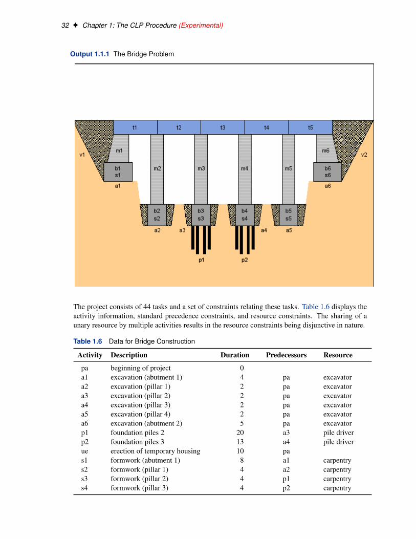
Example 1.1: Resource-Constrained Scheduling with NonstandardTemporal Constraints
This example illustrates a real-life scheduling problem and is used as a benchmark problem inthe CP community. The problem is to schedule the construction of a five-segment bridge (seeFigure 1.1.1). It comes from a Ph.D. dissertation on scheduling problems (Bartusch 1983).
32 F Chapter 1: The CLP Procedure (Experimental)
Output 1.1.1 The Bridge Problem
The project consists of 44 tasks and a set of constraints relating these tasks. Table 1.6 displays theactivity information, standard precedence constraints, and resource constraints. The sharing of aunary resource by multiple activities results in the resource constraints being disjunctive in nature.
s5 formwork (pillar 4) 4 a5 carpentrys6 formwork (abutment 2) 10 a6 carpentryb1 concrete foundation (abutment 1) 1 s1 concrete mixerb2 concrete foundation (pillar 1) 1 s2 concrete mixerb3 concrete foundation (pillar 2) 1 s3 concrete mixerb4 concrete foundation (pillar 3) 1 s4 concrete mixerb5 concrete foundation (pillar 4) 1 s5 concrete mixerb6 concrete foundation (abutment 2) 1 s6 concrete mixerab1 concrete setting time (abutment 1) 1 b1ab2 concrete setting time (pillar 1) 1 b2ab3 concrete setting time (pillar 2) 1 b3ab4 concrete setting time (pillar 3) 1 b4ab5 concrete setting time (pillar 4) 1 b5ab6 concrete setting time (abutment 2) 1 b6m1 masonry work (abutment 1) 16 ab1 bricklayingm2 masonry work (pillar 1) 8 ab2 bricklayingm3 masonry work (pillar 2) 8 ab3 bricklayingm4 masonry work (pillar 3) 8 ab4 bricklayingm5 masonry work (pillar 4) 8 ab5 bricklayingm6 masonry work (abutment 2) 20 ab6 bricklayingl delivery of the preformed bearers 2 cranet1 positioning (preformed bearer 1) 12 m1, m2, l cranet2 positioning (preformed bearer 2) 12 m2, m3, l cranet3 positioning (preformed bearer 3) 12 m3, m4, l cranet4 positioning (preformed bearer 4) 12 m4, m5, l cranet5 positioning (preformed bearer 5) 12 m5, m6, l craneua removal of the temporary housing 10v1 filling 1 15 t1 caterpillarv2 filling 2 10 t5 caterpillarpe end of project 0 t2, t3, t4, v1, v2, ua
A network diagram illustrating the precedence constraints in this problem is shown in Output 1.1.2.Each node represents an activity and gives the activity code, truncated description, duration, andthe required resource if any. The network diagram is generated using the NETDRAW procedure inSAS/OR software.
34 F Chapter 1: The CLP Procedure (Experimental)
Output 1.1.2 Network Diagram for the Bridge Construction Project
Bridge Construction Project
!"#$%&
&%& '(!)#*+
,!-.
/'-0#-%,#)1
23)!
&#
(##)#34%+
&/'!5
#63!,!4%
2#63!,!4+
!7#63!,!4%
2#63!,!4+
!8#63!,!4%
5#63!,!4+
!9#63!,!4%
2#63!,!4+
!2#63!,!4%
2#63!,!4+
!/#63!,!4%
7#63!,!4+
:5;+)*
<+)=
73!) #&4)
2;+(&0!4%
/9 %-#>0)%
:8;+)*
<+)=
/'3!) #&4)
/;+(&0!4%
2' %-#>0)%
:2;+)*
<+)=
73!) #&4)
:/;+)*
<+)=
?3!) #&4)
"53+&3)#4#
/3+&3)#4#
:7;+)*
<+)=
73!) #&4)
"83+&3)#4#
/3+&3)#4#
:9;+)*
<+)=
73!) #&4)
"23+&3)#4#
/3+&3)#4#
"/3+&3)#4#
/3+&3)#4#
!"5
3+&3)#4#
/"73+&3)#4#
/3+&3)#4#
!"8
3+&3)#4#
/"93+&3)#4#
/3+&3)#4#
!"2
3+&3)#4#
/!"/
3+&3)#4#
/
*5*!
:+&)1.
?")%3=
-!1
!"7
3+&3)#4#
/*8*!
:+&)1.
2'")%3=
-!1
!"9
3+&3)#4#
/*2*!
:+&)1.
?")%3=
-!1
*/*!
:+&)1.
/8")%3=
-!1
*7*!
:+&)1.
?")%3=
-!1
45 +
:%4%+&
/2 3)!&#*9
*!:+&)1.
?")%3=
-!1
4/ +
:%4%+&
/2 3)!&#
47 +
:%4%+&
/2 3)!1
+:%4%+&
/2 3)!&#,2 ;%--%&$
./'
3!4#) %-
42 +
:%4%+&
/2 3)!&#,/ ;%--%&$
./5
3!4#) %-
##&0.+;.
'
Example 1.1: Resource-Constrained Scheduling with Nonstandard Temporal Constraints F 35
In addition to the standard precedence constraints, there are the following constraints:
1. The time between the completion of a particular formwork and the completion of its corre-sponding concrete foundation is at most four days.
f .si/ � f .bi/ � 4; i D 1; � � � ; 6
2. There are at most three days between the end of a particular excavation (or foundation piles)and the beginning of the corresponding formwork.
f .ai/ � s.si/ � 3; i D 1; 2; 5; 6
and
f .p1/ � s.s3/ � 3
f .p2/ � s.s4/ � 3
3. The formworks must start at least six days after the beginning of the erection of the temporaryhousing.
s.si/ � s.ue/ C 6; i D 1; � � � ; 6
4. The removal of the temporary housing can start at most two days before the end of the lastmasonry work.
s.ua/ � f .mi/ � 2; i D 1; � � � ; 6
5. The delivery of the preformed bearers occurs exactly 30 days after the beginning of theproject.
s.l/ D s.pa/ C 30
The data set bridge defined by the SAS data set specification that follows, encapsulates all of theprecedence constraints and also indicates the resources required by each activity. Note the use ofthe reserved variables _ACTIVITY_, _SUCCESSOR_, _LAG_, and _LAGDUR_ to define the activityand precedence relationships. The list of reserved variables can be found in Table 1.5. The _RE-SOURCE_ variable is not used by the CLP procedure directly but used separately in a preprocessingstep to generate the RESOURCE statement for the CLP procedure.
data bridge;format _ACTIVITY_ $32. _DESC_ $34. _RESOURCE_ $14.
The edge-finder consistency algorithms are activated using the EDGEFINDER option in theSCHEDULE statement. The REQUIRES statement listing all the resources is generated via themacro variable reqstmt. The FINISH= option is specified to find a solution in 104 days, which alsohappens to be optimal.
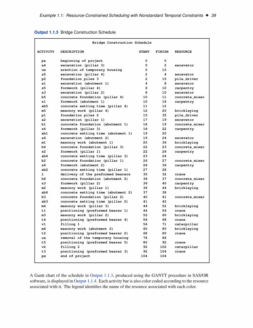
The sched_ex1 data set contains the complete schedule as computed by the CLP procedure, includ-ing the activity start and finish times and the assignment of resources. Since there is a variable foreach resource in this data set and an activity gets assigned to at most one resource, it is possible torepresent this information more concisely by merging the sched_ex1 data set with the desc data setby using the following statements. The resulting merged data set is shown in Output 1.1.3.
/* merge descriptions, prepare to output the schedule data set */proc sort data=sched_ex1;
by ACTIVITY;run;data sched_ex1;
merge desc sched_ex1;by ACTIVITY;
run;proc sort data=sched_ex1;
by START FINISH;run;
/* display the schedule */proc print data=sched_ex1 noobs width=min;
var ACTIVITY DESCRIPTION START FINISH RESOURCE;title ’Bridge Construction Schedule’;
run;
Example 1.1: Resource-Constrained Scheduling with Nonstandard Temporal Constraints F 39
Output 1.1.3 Bridge Construction Schedule
Bridge Construction Schedule
ACTIVITY DESCRIPTION START FINISH RESOURCE
pa beginning of project 0 0a4 excavation (pillar 3) 0 2 excavatorue erection of temporary housing 0 10a5 excavation (pillar 4) 2 4 excavatorp2 foundation piles 3 2 15 pile_drivera1 excavation (abutment 1) 4 8 excavators5 formwork (pillar 4) 6 10 carpentrya3 excavation (pillar 2) 8 10 excavatorb5 concrete foundation (pillar 4) 10 11 concrete_mixers1 formwork (abutment 1) 10 18 carpentryab5 concrete setting time (pillar 4) 11 12m5 masonry work (pillar 4) 12 20 bricklayingp1 foundation piles 2 15 35 pile_drivera2 excavation (pillar 1) 17 19 excavatorb1 concrete foundation (abutment 1) 18 19 concrete_mixers4 formwork (pillar 3) 18 22 carpentryab1 concrete setting time (abutment 1) 19 20a6 excavation (abutment 2) 19 24 excavatorm1 masonry work (abutment 1) 20 36 bricklayingb4 concrete foundation (pillar 3) 22 23 concrete_mixers2 formwork (pillar 1) 22 26 carpentryab4 concrete setting time (pillar 3) 23 24b2 concrete foundation (pillar 1) 26 27 concrete_mixers6 formwork (abutment 2) 26 36 carpentryab2 concrete setting time (pillar 1) 27 28l delivery of the preformed bearers 30 32 craneb6 concrete foundation (abutment 2) 36 37 concrete_mixers3 formwork (pillar 2) 36 40 carpentrym2 masonry work (pillar 1) 36 44 bricklayingab6 concrete setting time (abutment 2) 37 38b3 concrete foundation (pillar 2) 40 41 concrete_mixerab3 concrete setting time (pillar 2) 41 42m4 masonry work (pillar 3) 44 52 bricklayingt1 positioning (preformed bearer 1) 44 56 cranem3 masonry work (pillar 2) 52 60 bricklayingt4 positioning (preformed bearer 4) 56 68 cranev1 filling 1 56 71 caterpillarm6 masonry work (abutment 2) 60 80 bricklayingt2 positioning (preformed bearer 2) 68 80 craneua removal of the temporary housing 78 88t5 positioning (preformed bearer 5) 80 92 cranev2 filling 2 92 102 caterpillart3 positioning (preformed bearer 3) 92 104 cranepe end of project 104 104
A Gantt chart of the schedule in Output 1.1.3, produced using the GANTT procedure in SAS/ORsoftware, is displayed in Output 1.1.4. Each activity bar is also color coded according to the resourceassociated with it. The legend identifies the name of the resource associated with each color.
40 F Chapter 1: The CLP Procedure (Experimental)
Output 1.1.4 Gantt Chart for the Bridge Construction Project
PROC CLP - Solution to Bridge Problem
:104 days (optimal)
N/A
bricklaying
carpentry
caterpillar
concrete_mixer
crane
excavator
pile_driver
Resource Used
!
" "!
# #!
$ $!
% %!
! !!
& &!
' '!
( (!
) )!
"
" !
*+,-.
-,/0,
*1,
2-3-04
56777777
6%777777
#
89777777
"
6!777777
#%
5#777777
#"!
6"777777
%(
:!777777
&"
6$777777
("
;!777777
" ""
:"777777
" "(
6;!77777
"""#
<!777777
"##
5"777777
"!$!
6#777777
"'")
;"777777
"(")
:%777777
"(##
6;"77777
")#
6&777777
")#%
<"777777
# $&
;%777777
###$
:#777777
###&
6;%77777
#$#%
;#777777
#&#'
:&777777
#&$&
6;#77777
#'#(
=7777777
$ $#
;&777777
$&$'
:$777777
$&%
<#777777
$&%%
6;&77777
$'$(
;$777777
% %"
6;$77777
%"%#
<%777777
%%!#
>"777777
%%!&
<$777777
!#&
>%777777
!&&(
?"777777
!&'"
<&777777
& (
>#777777
&((
86777777
'(((
>!777777
( )#
?#777777
)#"
#>$777777
)#"
%59
777777
" %
" %
Example 1.2: Scheduling with Alternate Resources F 41
Example 1.2: Scheduling with Alternate Resources
This example shows an interesting job shop scheduling problem illustrating the use of alternativeresources. There are 90 jobs (J1–J90) that need to be processed on one of 10 machines (M0–M9).Not every machine can process every job. In addition, certain jobs might also require one of 7operators (OP0–OP6). As with the machines, not every operator can be assigned to every job.There are no explicit precedence relationships in this example.
The machine and operator requirements for each job are specified within the data set proj by usingthe following statements.
Each row in the datalines section defines a resource requirement for up to three jobs that are iden-tified in the variables j1–j3. The resource requirement associated with each of these jobs is a set ofalternates and is defined using the variables m1–m3 and o1–o4.
The variables m1–m3 represent a machine or workstation ID that the job needs to be processedon, and the variables o1–o4 represent an operator ID. The duration of each of the jobs identifiedin j1–j3 is assumed to be identical and defined using the dur variable. Each of the jobs in a rowcan be processed on any one of the machines in m1–m3 and requires the assistance of one of theoperators in o1–o4 while being processed. In other words, the resource requirement for each jobis a conjunction of disjunctive requirements (or alternates). A job requires one of m1–m3 and oneof o1–o4 in order to be processed. For example, observation 5 specifies that job number 7 can beprocessed on either machine 6, 7, or 8 and additionally requires either operator 5 or operator 6 inorder to be processed. The next observation indicates that jobs 8 and 9 can also be processed on thesame set of machines. However, they do not require any operator assistance.
Example 1.2: Scheduling with Alternate Resources F 43
The ACTIVITY and REQUIRES statements for the CLP procedure are next generated from thedata set proj by the following program:
/* generate the ACTIVITY and REQUIRES statements */data _null_;
set proj end=finish;format jobs $32. resources $char128.;format acts reqs $char4096.;retain acts reqs;array v{11} j1-j3 m1-m3 o1-o4 dur;jobs=catx(’ J’,of j1-j3);acts=catx(’ ’,acts,cats(’(J’,jobs,’)=’,’(’,dur,’)’));do i=4 to 6;
if v{i}=’ ’ then leave;if v{7}=’ ’ then resources=catx(’,’,resources,’M’||v{i});else do j=7 to 10;
if v{j}=’ ’ then leave;resources=catx(’,’,resources,catx(’ ’,’M’||v{i},’OP’||v{j}));end;
end;reqs=catx(’ ’,reqs,cats(’(J’,jobs,’)=’,’(’,resources,’)’));if finish then do;call symput(’activities’,strip(acts));call symput(’requirements’,strip(reqs));end;
run;
The CLP procedure is invoked by using the following statements with DUR=12 to obtain a 12-daysolution that is also known to be optimal.
/* invoke PROC CLP to find a schedule */proc clp dom=[0,12] scheddata=sched_ex2 restarts=500 dpr=25;
The activity selection strategy is one that selects a maximum duration activity at random from thesubset of activities that begin prior to the earliest early finish time. This strategy is specified usingthe ACTSELECT=MAXD option on the SCHEDULE statement.
The resulting schedule is shown in a series of Gantt charts that are displayed in Output 1.2.1 andOutput 1.2.2. In each of these Gantt charts, the vertical axis lists the different jobs, the horizontalbar represents the start and finish times for each of the jobs, and the text above each bar identifiesthe machine that the job is being processed on. Output 1.2.1 displays the schedule for the operator-assisted tasks—one for each operator. Output 1.2.2 shows the schedule for automated tasks—thatis, those tasks not requiring operator intervention.
44 F Chapter 1: The CLP Procedure (Experimental)
Output 1.2.1 Operator-Assisted Jobs Schedule
Schedule for Operator OP0 !"#$%&'()&%*$+$&)',-./&'0!1
2 3 4 5 6 7 8 9 : ; 32 33 34<=0
<45<75<43<4'<3'<::<5;<8;<5:
4 7
3 3
2 5
3 6
2
Schedule for Operator OP1 !"#$%&'()&%*$+$&)',-./&'0!1
2 3 4 5 6 7 8 9 : ; 32 33 34<=0
<93<44<74<92<5'<36<72<6;<:;
7 3
6 7
4 9
7 7
6
Example 1.2: Scheduling with Alternate Resources F 45
Output 1.2.1 continued
Schedule for Operator OP2 !"#$%&'()&%*$+$&)',-./&'0!1
2 3 4 5 6 7 8 9 : ; 32 33 34<=0
<94<69<95<73<6:<8:<62<;2
5 5
5 6
4 4
4 7
Schedule for Operator OP3 !"#$%&'()&%*$+$&)',-./&'0!1
2 3 4 5 6 7 8 9 : ; 32 33 34<=0
<54<89<6'<33<35<8'<4;<:7<34<7;
6 4
7 4
; 7
6 2
9 4
46 F Chapter 1: The CLP Procedure (Experimental)
Output 1.2.1 continued
Schedule for Operator OP4 !"#$%&'()&%*$+$&)',-./&'0!1
2 3 4 5 6 7 8 9 : ; 32 33 34<=0
<88<67<7:<7'<53<9;<52<9:<:8
2 2
4 7
5 2
5 2
3
Schedule for Operator OP5 !"#$%&'()&%*$+$&)',-./&'0!1
2 3 4 5 6 7 8 9 : ; 32 33 34<=0
<68<55<87<:9<96<37<49<82<9'
3 6
2 4
9 8
9 3
:
Example 1.2: Scheduling with Alternate Resources F 47
Output 1.2.1 continued
Schedule for Operator OP6 !"#$%&'()&%*$+$&)',-./&'0!1
A more interesting Gantt chart is that of the resource schedule by machine, as shown in Output 1.2.3.This chart displays the schedule for each machine. Every row corresponds to a machine. Every baron each row consists of multiple segments, and every segment represents a job that is processed onthe machine. Each segment is also coded according to the operator assigned to it. The mappingof the coding is indicated in the legend. It is evident that the schedule is optimal since none of themachines or operators are idle at any time during the schedule.
Example 1.3: 10×10 Job Shop Scheduling Problem F 49
Output 1.2.3 Another Gantt Chart: Proof of Optimality
Scheduling With Alternate Resouces !"#$%&#'()'*+!",-#
N/A OP0 OP1 OP2
OP3 OP4 OP5 OP6
Operator Required
. / 0 1 2 3 4 5 6 7 /. // /0*89:;<=
*.'''''*/'''''*0'''''
*1'''''*2'''''*3'''''*4'''''*5'''''
*6'''''*7'''''
>44 >23 >43 >6. >/ >57 >63 >56 >16
>24 >00 >0/ >0 >0. >/7 >17 >4. >64
>01 >45 >36 >// >65 >1 >26 >46 >2. >37
>50 >25 >51 >1/ >66 >1. >/6 >/5
>10 >11 >30 >3/ >07 >06 >47 >67
>5/ >31 >2 >3 >5. >4 >/4 >3. >27 >7.
>40 >4/ >6/ >04 >12 >/3 >13 >32 >53
>2/ >60 >20 >6 >52 >/2 >05 >/0 >34
>42 >61 >22 >54 >15 >35 >/. >7 >5
>41 >62 >21 >/1 >33 >02 >55 >03 >14
Example 1.3: 10×10 Job Shop Scheduling Problem
This example is a job shop scheduling problem from Lawrence (1984). This test is also known asLA19 in the literature, and its optimal solution is known to be 842 (Applegate and Cook 1991).There are 10 jobs (Job 1 – 10) and 10 machines (M0 – M9). Every job must be processed on eachof the 10 machines in a predefined sequence. The objective is to minimize the makespan. The jobsare described in the data set raw by using the following statements.
50 F Chapter 1: The CLP Procedure (Experimental)
/* jobs specification */data raw (drop=i mid);
do i=1 to 10;input mid _DURATION_ @;MACHINE=compress(’M’||mid);output;
Each row in the datalines section specifies a job by 10 pairs of consecutive numbers. Each pairof numbers defines one task of the job, which represents the processing of a job on a machine.For each pair, the first number identifies the machine it executes on and the second number is theduration. The order of the 10 pairs defines the sequence of the tasks for a job.
The following statements create the activity data set actdata.
/* create the activity data set */data actdata (drop= i j);
format _ACTIVITY_ $8. _SUCCESSOR_ $8.;set raw;i=mod(_n_-1,10)+1;j=int((_n_-1)/10)+1;_ACTIVITY_ = compress(’J’||j||’P’||i);JOB=j;TASK=i;if i LT 10 then
_SUCCESSOR_ = compress(’J’||j||’P’||(i+1));else
_SUCCESSOR_ = ’ ’;output;
run;
Had there been sufficient machine capacity, the jobs could have been processed according to aschedule as shown in Output 1.3.1. The minimum makespan would be 617—the times it takes tocomplete Job 1.
Example 1.3: 10×10 Job Shop Scheduling Problem F 51
Output 1.3.1 Gantt Chart: Schedule for the Unconstrained Problem
10X10 Job Shop Scheduling Problem !"#!$%&'(!)*+,"-)*./)
M0 M1 M2 M3 M4
M5 M6 M7 M8 M9
Machine Required
0 10 230 240 350 600 610 530 540 750 100 11089:
236571;4<20
30 12;
This schedule will be infeasible when there is only a single instance of each machine. For example,at time period 20, the schedule requires two instances of each of the machines M6, M7, and M9.
In order to solve the resource-constrained schedule, the CLP procedure is invoked by using thefollowing statements.
The edge-finder algorithm is activated with the EDGEFINDER option in the SCHEDULE state-ment. In addition, the edge-finding extensions for detecting whether a job cannot be the first orcannot be the last to be processed from a subset of jobs to be processed on a particular machineare invoked with the NF= and NL= options, respectively, in the SCHEDULE statement. The de-fault activity selection and activity assignment strategies are used. A restart heuristic is used asthe look-back method to handle recovery from failures. The DPR= option specifies that a totalrestart be performed after encountering 50 failures, and the RESTARTS= option limits the numberof restarts to 500. The REQUIRES statement for the CLP procedure is generated via the macrovariable reqstmt.
The resulting 842-time-period schedule is displayed in Output 1.3.2. Each row represents a job.Each segment represents a task (the processing of a job on a machine), which is also coded accordingto the executing machine. The mapping of the coding is indicated in the legend. Note that nomachine is used by more than one job at any point in time.
ReferencesApplegate, D. and Cook, W. (1991), “A Computational Study of the Job Shop Scheduling Problem,”
ORSA Journal on Computing, 3, 149–156.
Baptiste, P. and Le Pape, C. (1996), “Edge-Finding Constraint Propagation Algorithms for Dis-junctive and Cumulative Scheduling,” in Proceedings of the 15th Workshop of the UK PlanningSpecial Interest Group, Liverpool, UK.
Bartusch, M. (1983), Optimierung von Netzplänen mit Anordnungsbeziehungen bei knappen Be-triebsmitteln, Ph.D. thesis, Universität Passau, Fakultät für Mathematik und Informatik.
Carlier, J. and Pinson, E. (1989), “An Algorithm for Solving the Job-Shop Scheduling Problem,”Management Science, 35(2), 164–176.
Carlier, J. and Pinson, E. (1990), “A Practical Use of Jackson’s Preemptive Schedule for Solvingthe Job-Shop Problem,” Annals of Operations Research, 26, 269–287.
54 F Chapter 1: The CLP Procedure (Experimental)
Colmerauer, A. (1990), “An Introduction to PROLOG III,” Communications of the ACM, 33, 70–90.
Floyd, R. W. (1967), “Nondeterministic Algorithms,” Journal of the ACM, 14, 636–644.
Garey, M. R. and Johnson, D. S. (1979), Computers and Intractability: A Guide to the Theory ofNP-Completeness, New York: W. H. Freeman & Co.
Haralick, R. M. and Elliot, G. L. (1980), “Increasing Tree Search Efficiency for Constraint Satis-faction Problems,” Artificial Intelligence, 14, 263–313.
Jaffar, J. and Lassez, J. (1987), “Constraint Logic Programming,” Conference Record of the 14thAnnual ACM Symposium in Principles of Programming Languages, Munich, 111–119.
Kumar, V. (1992), “Algorithms for Constraint-Satisfaction Problems: A Survey,” AI Magazine, 13,32–44.
Lawrence, S. (1984), Resource Constrained Project Scheduling: An Experimental Investigation ofHeuristic Scheduling Techniques (Supplement), Pittsburgh: Graduate School of Industrial Ad-ministration, Carnegie Mellon University.
Mackworth, A. K. (1977), “Consistency in Networks of Relations,” Artificial Intelligence, 8, 99–118.
Muth, J. F. and Thompson, G. L., eds. (1963), Industrial Scheduling, Englewood Cliffs, NJ: PrenticeHall.
Nemhauser, G. L. and Wolsey, L. A. (1988), Integer and Combinatorial Optimization, New York:John Wiley & Sons.
Nuijten, W. (1994), Time and Resource Constrained Scheduling, Ph.D. thesis, Eindhoven Instituteof Technology.
Smith, B. M., Brailsford, S. C., Hubbard, P. M., and Williams, H. P. (1996), “The Progressive PartyProblem: Integer Linear Programming and Constraint Programming Compared,” Constraints, 1,119–138.
Tsang, E. (1993), Foundations of Constraint Satisfaction, London: Academic Press.
Van Hentenryck, P. (1989), Constraint Satisfaction in Logic Programming, Cambridge, MA: MITPress.
Van Hentenryck, P., Deville, Y., and Teng, C. (1992), “A Generic Arc-Consistency Algorithm andIts Specializations,” Artificial Intelligence, 57, 291–321.
Waltz, D. L. (1975), “Understanding Line Drawings of Scenes with Shadows,” in P. H. Winston,ed., The Psychology of Computer Vision, 19–91, New York: McGraw-Hill.
Williams, H. P. and Wilson, J. M. (1998), “Connections between Integer Linear Programming andConstraint Logic Programming—An Overview and Introduction to the Cluster of Articles,” IN-FORMS Journal of Computing, 10, 261–264.