Throughout coastal and ocean engineering the convenient model of a steadily-progressing periodic wavetrain is used to give fluid velocities, pressures and surface elevations caused by waves, even in situationswhere the wave is being slowly modified by effects of viscosity, current, topography and wind or wherethe wave propagates past a structure with little effect on the wave itself. In these situations the wavesdo seem to show a surprising coherence of form, and they can be modelled by assuming that they arepropagating steadily without change, giving rise to the so-called steady wave problem, which can beuniquely specified and solved in terms of three physical length scales only: water depth, wave lengthand wave height. In practice, the knowledge of the detailed flow structure under the wave is so importantthat it is usually considered necessary to solve accurately this otherwise idealised model.
The main theories and methods for the steady wave problem which have been used are: Stokes theory,an explicit theory based on an assumption that the waves are not very steep and which is best suitedto waves in deeper water; cnoidal theory, an explicit theory for waves in shallower water; and Fourierapproximation methods which are capable of high accuracy but which solve the problem numericallyand require computationally-expensive matrix techniques. A review and comparison of the methods isgiven in Sobey, Goodwin, Thieke & Westberg (1987) and Fenton (1990). For relatively simple solutionmethods that are explicit in nature, Stokes and cnoidal theories have important and complementary rolesto play, and indeed it has relatively recently been shown that they are more accurate than has beenrealised (Fenton 1990).
This Chapter describes cnoidal theory and its application to practical problems. It has probably notbeen applied as often as it might. One reason is the unfamiliarity of the Jacobian elliptic functions andintegrals and perceived difficulties in dealing with them. One possibility might be too that in the longwave limit for which the cnoidal theory is meant to apply, almost all expressions for elliptic functionsand integrals given in standard texts are very slowly convergent, for example, those in Abramowitz &Stegun (1965). Both of these factors need not be a disincentive; relatively recently some remarkableformulae have been given ( Fenton & Gardiner-Garden 1982) which are simple, short, and convergemost quickly in the limit corresponding to cnoidal waves. These will be presented below.
It may be, however, that the author has inadvertently provided further reasons for not preferring cnoidaltheory. In Fenton (1979) he presented a fifth-order cnoidal theory which was both apparently compli-cated, requiring the presentation of many coefficients as unattractive floating point numbers, and alsogave poor results for fluid velocities under high waves. In a later work ( Fenton 1990), however, the au-thor showed that instead of fluid velocities being expressed as expansions in wave height, if the originalspirit of cnoidal theory were retained and they be written as series in shallowness, then the results areconsiderably more accurate. Also in that work it was shown that, in the spirit of Iwagaki (1968), theseries can be considerably shortened and simplified by a good approximation.
There have been many presentations of cnoidal theory, most with essentially the same level of approxi-mation, and with relatively little to distinguish the essential common nature of the different approaches.However, there has been such a plethora of different notations, expansion parameters, definitions ofwave speed, and so on, that the practitioner could be excused for thinking that the whole field was verycomplicated. The aim of this article is to review developments in cnoidal theory and to present the mostmodern theory for practical use, together with a number of practical aids to implementation. My hopeis that this surprisingly simple and accurate theory becomes accessible to practitioners and regains itsrightful place in the study of long waves.
Initially a history of cnoidal theory is given, and various contributions are described and reviewed. Then,the theory which can be used to generate high-order solutions is outlined and theoretical results fromthat theory are presented. This chapter contains the first full presentation of those results in terms ofrational numbers, as previous versions have used some floating point numbers. Two forms of the theoryare presented: the first is a full third-order theory, the second is a fifth-order theory in which a coherentapproximation is introduced which, it is suggested, is accurate for most cases where cnoidal theory isused. It is suggested that this be termed the ”Iwagaki Approximation”. Next a detailed procedure for theapplication of the cnoidal theory is presented, allowing for cases where wavelength or period is specified.
2
Some new simplifications are introduced here. A number of practical tools and hints for the applicationof the theory are presented, including a numerical check on the coefficients used in this paper, a simpletest to check that the series are correct as programmed by the user, some simple approximations arepresented for the elliptic functions and integrals used, and techniques for convergence enhancement ofthe series are described. A numerical cnoidal theory developed by the author is then presented, which isa numerical method based on cnoidal theory. Finally, the accuracies of the methods are examined andappropriate limits are suggested.
Background
There have been many books and articles written on the propagation of surface gravity waves. Thesimplest theory is conventional long-wave theory, which assumes that pressure at every point is equal tothe hydrostatic head at that point, and which gives the result that any finite amplitude disturbance muststeepen until the assumptions of the theory break down. Unsettling evidence that this is not the case wasprovided by the publication in 1845 by John Scott Russell of his observations on the ”great solitary waveof translation” generated by a canal barge and seeming to travel some distance without modification.This was derided by Airy (”We are not disposed to recognize this wave as deserving the epithets ’great’or ’primary’ ...”, ( Rayleigh 1876)) who believed that it was nothing new and could be explained bylong-wave theory. This is one aspect of the long-wave paradox, later resolved by Ursell (1953), whoshowed the importance of a parameter that incorporates the height and length of disturbance and thewater depth in determining the behaviour of waves. The value of the parameter determines whether theyare true long waves and show the steepening behaviour, or whether they are ”not-so-long” waves wherepressure and velocity variation over the depth is more complicated, as is their behaviour. The cnoidaltheory fits into this latter category.
Boussinesq (1871) and Rayleigh (1876) introduced an expansion based on the waves being long relativeto the water depth. They showed that a steady wave of translation with finite amplitude could be obtainedwithout making the linearising assumption, and that the waves were inherently nonlinear in nature. Thesolutions they obtained assumed that the water far from the wave was undisturbed, so that the solutionwas a solitary wave, theoretically of infinite length. Cnoidal theory obtained its name in 1895 whenKorteweg & de Vries (1895) obtained their eponymous equation for the propagation of waves over aflat bed, using a similar approximation to Boussinesq and Rayleigh. However they obtained periodicsolutions which they termed ”cnoidal” because the surface elevation is proportional to the square of theJacobian elliptic function cn(). The cnoidal solution shows the familiar long flat troughs and narrowcrests of real waves in shallow water. In the limit of infinite wavelength, it describes a solitary wave.
Since Korteweg and de Vries there have been a number of presentations of cnoidal theory. Keulegan& Patterson (1940), Keller (1948), and Benjamin & Lighthill (1954) have presented first-order theo-ries. The latter is particularly interesting, in that it relates the wave dimensions to the volume flux,energy and momentum of a flow in a rectangular channel (or per unit width over a flat bed) and showedthat waves of cnoidal form could approximate an undular hydraulic jump. Wiegel (1960, 1964) gavea detailed presentation of first-order theory with a view to practical application, including details ofmathematical approximations to the elliptic integrals. A second-order cnoidal theory was presented ina formal manner by Laitone (1960, 1962) who provided a number of results, re-casting the series interms of the wave height/depth. However, the second-order results are surprisingly inaccurate for highwaves (see, for example, Le Méhauté, Divoky & Lin (1968)). The next approximation was obtainedby Chappelear (1962), as one of a remarkable sequence of papers on nonlinear waves. He obtained thethird-order solution, and expressed the results as series in a parameter directly proportional to shallow-ness: (depth/wavelength)2.
Iwagaki published his ”Hyperbolic theory” in 1967, with an English version appearing a year later,Iwagaki (1968). This was an interesting development, for it was an attempt to make the computation ofthe elliptic functions and integrals simpler by replacing all of them by their limiting behaviours in thelimit of solitary waves, except for quantities related to wavelength. In this case, the cn function becomesthe hyperbolic secant function sech, and other elliptic functions become other hyperbolic functions,
3
giving rise to the name he proposed. This approach raises a number of interesting points, and furtherbelow we will discuss it in some detail.
Tsuchiya and Yasuda in 1974, with an English version in 1985 (Tsuchiya & Yasuda 1985), obtained athird-order solution with the introduction of another definition of wave celerity based on assumptionsconcerning the Bernoulli constant. Nishimura, Isobe & Horikawa (1977) devised procedures for gen-erating high-order theories for both Stokes and cnoidal theories, making extensive use of recurrencerelations. The authors concentrated on questions of the convergence of the series. They computed a24th-order solution, however, few detailed formulae for application were given.
The author (Fenton 1979) produced a method in 1979 for the computer generation of high-order cnoidalsolutions for periodic waves. It had been observed that second-order solutions for fluid velocity werequite inaccurate (Le Méhauté et al. 1968), and it was desired to produce more accurate results, as wellas trying to make the method more readily available for practical application. Like Laitone resultswere expressed in terms of the relative wave height. The paper also raised some interesting points:how it is rather simpler to use the trough depth as the depth scale in presenting results, and that theeffective expansion parameter is not simply the wave height but is actually the wave height dividedby the elliptic parameter m. For the expansion parameter to be small and for the series results to bevalid, the short wave limit is excluded. In this way the cnoidal theory breaks down in deep water (shortwaves) in a manner complementary to that in which Stokes theory breaks down in shallow water (longwaves) (Fenton 1985). A solution was presented to fifth order in wave height, with a large number ofnumerical coefficients in floating point form. For moderate waves, results were good when comparedwith experiment, but for higher waves the velocity profile showed exaggerated oscillations and it wasfound that ninth-order results were worse. These results were unexpectedly poor.
Isobe, Nishimura & Horikawa (1982) continued the work of Nishimura et al. (1977) and presented aunified view of Stokes and cnoidal theories. They proposed a generalised double series expansion interms of Ursell parameter and shallowness, the square of the ratio of water depth to wavelength. Theyalso proposed a boundary between areas of application of Stokes and cnoidal theory of U = 25, whereU is the Ursell number,Hλ2/d3.
In a review article in 1990, the author (Fenton 1990) considered cnoidal theory as well as Stokes theoryand Fourier approximation methods such as the ”stream function method”. The approach to cnoidaltheory in Fenton (1979) was re-examined and some useful advances made. It was found that if theseries for velocity were expressed in terms of the shallowness rather than relative wave height, as doneby Chappelear (1962), then results were very much better, and justified the use of cnoidal theory evenfor high waves. This would fit in with the fundamental approximation of the cnoidal theory being anexpansion in shallowness. That review article also incorporated the fact that the wave theory does notdetermine the wave speed, and that neither Stokes’ first nor second definitions of velocity are necessarilycorrect. In general it is necessary to incorporate the effects of current, as had been done using graphicalmeans in Jonsson, Skougaard & Wang (1970) and Hedges (1978), and analytically for numerical wavetheories in Rienecker & Fenton (1981) and for high-order Stokes theory in Fenton (1985).
We now present the theory and results. The theory is essentially that described in Fenton (1979) butwith the advances made in Fenton (1990) incorporated plus some more contributions introduced in thischapter. A number of suggestions for practical use are made, and then the performance of the theory iscompared with other methods. One of those is a new numerical version of cnoidal theory. In general,the theory as presented here is found to be surprisingly robust and accurate over a wide range of waves.
Cnoidal theory
The physical problem
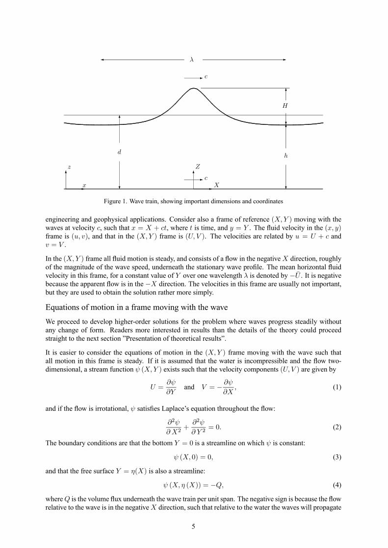
Consider the wave as shown in Figure 1, with a stationary frame of reference (x, y), x in the directionof propagation of the waves and y vertically upwards with the origin on the flat bed. The waves travelin the x direction at speed c relative to this frame. It is this frame which is the usual one of interest for
4
6
-x
z
6
- X
Z
- c
- c
d
6
?
λ¾ -
H
6
?
h
6
?
Figure 1. Wave train, showing important dimensions and coordinates
engineering and geophysical applications. Consider also a frame of reference (X,Y ) moving with thewaves at velocity c, such that x = X + ct, where t is time, and y = Y . The fluid velocity in the (x, y)frame is (u, v), and that in the (X,Y ) frame is (U, V ). The velocities are related by u = U + c andv = V .
In the (X,Y ) frame all fluid motion is steady, and consists of a flow in the negativeX direction, roughlyof the magnitude of the wave speed, underneath the stationary wave profile. The mean horizontal fluidvelocity in this frame, for a constant value of Y over one wavelength λ is denoted by −U . It is negativebecause the apparent flow is in the −X direction. The velocities in this frame are usually not important,but they are used to obtain the solution rather more simply.
Equations of motion in a frame moving with the wave
We proceed to develop higher-order solutions for the problem where waves progress steadily withoutany change of form. Readers more interested in results than the details of the theory could proceedstraight to the next section ”Presentation of theoretical results”.
It is easier to consider the equations of motion in the (X,Y ) frame moving with the wave such thatall motion in this frame is steady. If it is assumed that the water is incompressible and the flow two-dimensional, a stream function ψ (X,Y ) exists such that the velocity components (U,V ) are given by
U =∂ψ
∂Yand V = − ∂ψ
∂X, (1)
and if the flow is irrotational, ψ satisfies Laplace’s equation throughout the flow:
∂2ψ
∂X2+
∂2ψ
∂ Y 2= 0. (2)
The boundary conditions are that the bottom Y = 0 is a streamline on which ψ is constant:
ψ (X, 0) = 0, (3)
and that the free surface Y = η(X) is also a streamline:
ψ (X, η (X)) = −Q, (4)
whereQ is the volume flux underneath the wave train per unit span. The negative sign is because the flowrelative to the wave is in the negativeX direction, such that relative to the water the waves will propagate
5
in the positive x direction. The remaining boundary condition comes from Bernoulli’s equation:
1
2
¡U2 + V 2
¢+ gy +
p
ρ= R, (5)
in which g is gravitational acceleration, p is pressure, ρ is density and R is the Bernoulli constant forthe flow, the energy per unit mass. If equation (5) is evaluated on the free surface Y = η(X), on whichpressure p = 0, we obtain
1
2
õ∂ψ
∂X
¶2+
µ∂ ψ
∂Y
¶2!¯¯Y=η
+ gη = R, (6)
We assume a Taylor expansion for ψ about the bed of the form:
ψ = − sinY d
dX. f (X) = −Y df
dX+Y 3
3!
d3f
dX3− . . . , (7)
as in Fenton (1979), where df/dX is the horizontal velocity on the bed. We have introduced the infinitedifferential operator sinY d/dX as a convenient way of representing the infinite Taylor series, whichhas significance only as its power series expansion
sinYd
dx= Y
d
dx− Y
3
3!
d3
dx3+Y 5
5!
d5
dx5− . . . .
It can be shown that the velocity components anywhere in the fluid are
U =∂ψ
∂Y= − ∂
∂YsinY
d
dX. f (X) = − cosY d
dX. f 0(X),
V = − ∂ψ
∂X=
∂
∂XsinY
d
dX. f (X) = sinY
d
dX. f 0(X), (8)
Further differentiation shows that the assumption of equation (7) satisfies the field equation (2) and thebottom boundary condition (3). The kinematic surface boundary condition (4) becomes
sin ηd
dX. f (X) = Q, (9)
This equation is a nonlinear ordinary differential equation of infinite order for the local fluid depth η andf 0 (X), the local fluid velocity on the bed, in terms of the horizontal coordinateX.
The remaining equation is the dynamic free surface condition, equation (6). Substituting equation (8)evaluated on the free surface we obtain:
1
2
õcos η
d
dX.df
dX
¶2+
µsin η
d
dX.df
dX
¶2!+ gη = R. (10)
One of the squares of the infinite order operators can be eliminated by differentiating (9):
sin ηd
dX.df
dX+dη
dXcos η
d
dX.df
dX=dQ
dX= 0,
as Q is constant along the channel, to give
1
2
Ã1 +
µdη
dX
¶2!µcos η
d
dX.df
dX
¶2+ gη = R. (11)
Equations (9) and (11) are two nonlinear ordinary differential equations in the unknowns η(X) andf 0(X), the horizontal velocity on the bed. They are of infinite order, and will have to be approximatedin some way. It is possible that they could be solved as differential equations, but that would require aninfinite number of boundary conditions. In this and subsequent sections we use two methods, one usingpower series solution methods, the traditional way, and another using a numerical spectral approachbased on assuming series of known functions.
6
Series solution
The equations have the trivial solution of uniform flow with constant depth: η = h and f 0(X) = U . Weproceed to a series expansion about the state of a uniform critical flow. We will assume that all variationin X is relatively slow and can be expressed in terms of a scaled dimensionless variable αX/h, whereα is a small quantity which expresses the relative slowness of variation in the X direction, and h is theminimum or trough depth of fluid. At this stage, while solving the equations, it is more convenient towrite them in terms of dimensionless variables. We let the scaled horizontal variable be θ = αX/h.Writing η∗ = η/h and f∗ = f/Q, equation (9) can be written
1
αsin η∗α
d
dθ. f∗ − 1 = 0. (12)
The dynamic boundary condition (11) can be written in terms of these quantities as
1
2
Ã1 + α2
µdη∗dθ
¶2!µcos η∗α
d
dθ. f 0∗(θ)
¶2+ g∗η∗ = R∗, (13)
where g∗ = gh3/Q2 is a dimensionless gravity number (actually the inverse square of the Froude num-ber) and R∗ = Rh2/Q2 is a dimensionless Bernoulli constant.
The form of equations (12) and (13) suggests that we use α2 as the expansion parameter. We write theseries expansions
η∗ = 1 +NXj=1
α2jYj (θ) , (14)
f 0∗ = 1 +NXj=1
α2jFj (θ) , (15)
g∗ = 1 +NXj=1
α2jgj , (16)
R∗ =3
2+
NXj=1
α2jrj , (17)
where N is the order of solution required. Now, these are substituted into equations (12) and (13).Grouping all the terms in α0, α2, α4, . . ., and requiring that the coefficient equation of each be satisfiedidentically, a hierarchy of equations is obtained which can be solved sequentially. At α0 the equationsare satisfied identically; at α2 we obtain
F1 + Y1 = 0,
F1 + Y1 + g1 − r1 = 0,
with solution Y1 = −F1 and g1 = r1. At the next order α4 we obtain
F2 + Y2 + F1Y1 − 16F 001 = 0,
F2 + Y2 + g2 − r2 − 12F 001 +
1
2F 21 + g1Y1 = 0,
and by subtracting one from the other, and using information from the previous order, we obtain
1
3F 001 −
3
2F 21 + r2 − g2 + g1F1 = 0. (18)
This is a differential equation of second order which is nonlinear because of the F 21 term. The usualway of integrating such an equation (for example, #3.3.3of Shen 1993) is to write the F 001 term as
7
d(F 021 /2)/dF1, integrate the equation with respect to F1, from which the solution for F1 in terms ofcn2(θ|m), a Jacobian elliptic function (see, for example, #16 of Abramowitz & Stegun 1965), can beobtained. This is a rather complicated procedure. Here we prefer a rather simpler approach to solve thenonlinear differential equation by presuming knowledge of the nature of the solution. We write
F1 = A1 cn2(θ|m), (19)
where A1 is independent of θ, andm is the parameter of the elliptic function. Using the properties as setout in Abramowitz & Stegun (1965), (#16.9 and #16.16), reproduced as equations (40) and (41) below,it can be shown that
Substituting into equation (18) and collecting coefficients of powers of cn2 (θ|m) we obtain:
A1 = −43m, g1 =
4
3(1− 2m) , r2 − g2 = 8
9m (1−m) ,
such that the first-order cnoidal solution is
η∗ = 1 + α24
3m cn2 (θ|m) ,
f 0∗ = 1− α24
3m cn2 (θ|m) ,
g∗ = 1 + α24
3(1− 2m) ,
R∗ =3
2+ α2
8
9m (1−m) . (21)
These solutions should have been shown with order symbols O¡α4¢
after them, showing that the ne-glected terms are at least of the order of α4. As this is obvious anyway, we choose not to do that here orelsewhere in this work, where the order of neglected terms is almost everywhere obvious.
The procedure described here can be repeated at all orders of α2, and at each higher order a differentialequation is obtained which is linear in the unknowns, and with increasingly complicated and lengthyterms involving the already-known lower orders of solution. The procedure has been described in somedetail in Fenton (1979). At each order j, the solution for Fj and Yj involves polynomials in cn2 (θ|m)of degree j. With increasing complexity, the operations quickly become too lengthy for hand calculationand it is necessary to use computer software. In the 1979 paper floating point arithmetic and a conven-tional language (FORTRAN) was used, however now, at the time of writing of this chapter, it is mucheasier to use modern software which can perform mathematical manipulations. In the preparation of thisarticle the author used the symbolic manipulation software MAPLE.
After the operations have been completed, the solutions which are to hand are power series in α2, up tothe order desired, for η∗, f 0∗, g∗ and R∗. It is convenient to obtain the series for Q/
pgh3 by taking the
power series of g−1/2∗ and the series for R/gh by taking the power series of R∗/g∗, and the series forψ/pgh3 by taking the power series of ψ∗ ×Q/
pgh3, where ψ∗ is evaluated from
ψ∗ = −1
αsin η∗α
d
dθ. f∗. (22)
Expressions for velocity components follow by differentiation.
So far, all series have been in terms of α2. It is simpler to express the series in terms of δ, where
δ = 4α2/3, (23)
as suggested by the results of equation (21). Physical solutions could be presented in terms of thesepower series, and they do reflect the nature of the theory, that the essential nature of the approximationis that the waves be long (α small). However the majority of presentations have converted to expansions
8
in terms of ε = H/h, the ratio of wave height to trough depth. This can be done by expressing a seriesfor ε in terms of δ or α2 by evaluating η∗ − 1 with cn = 1. The series can then be reverted to express δor α2 in terms of ε, which can then be substituted.
The parameterm is determined by the geometry of the wave. As the function cn (θ|m) has a real periodof 4K(m), where K is the complete elliptic integral of the first kind, ( Abramowitz & Stegun 1965),it is easily shown that cn2 (θ|m) has a period of 2K(m), and as the wave has a wavelength of λ theelementary geometric relation holds:
αλ
h= 2K(m). (24)
The mean depth d is known in physical problems, but it has not entered the calculations yet. The ratiod/h can be obtained from the series for η∗ = η/h, by replacing each cn2j by Ij where Ij is the meanvalue of cn2j (θ|m):
Ij = cn2j (θ|m), (25)
then, (#5.13 of Gradshteyn & Ryzhik 1965): I0 = 1, I1 = (−1 + m + e(m))/m, where e(m) =E(m)/K(m), and E(m) is the complete elliptic integral of the second kind, and the other values maybe computed from
Ij+2 =
µ2j + 2
2j + 3
¶µ2− 1
m
¶Ij+1 +
µ2j + 1
2j + 3
¶µ1
m− 1¶Ij , for all j. (26)
This allows all quantities to be calculated with d as the non-dimensionalising depth scale. Similarly themean fluid speed: U/
√gh,which is related to wave speed, can be obtained from the series for horizontal
velocity U/√gh, by replacing each cn2j by Ij .
Presentation of theoretical results
Two sets of results are presented here. For the first time a complete solution is given in terms of rationalnumbers, whereas in Fenton (1990) at least some floating-point numbers were used. Firstly, a fullsolution is presented to third-order, which is a reasonable limit for space reasons. Next, a fifth-ordersolution is presented, but in which the approximation is made of setting the parameter m to 1 whereverit explicitly occurs in the coefficients of the series expansions. This makes feasible the presentation of thetheory to two higher orders. Here we present the solutions; the application and use of these theoreticalresults will be described in the subsequent section.
Features of solutions
Although the underlying method relies on an expansion in shallowness, it is often convenient to presentresults in terms of expansions in wave height. It was found in Fenton (1979) that the best parameter forthis was the wave height relative to the trough depth, H/h, which we denote by ε. If the mean depthhad been used, to give a series inH/d, many more terms would be involved, because, as equation (A.8)shows, the expression for h/d involves a double polynomial inm and e = E/K of degree n at order n,such that, for example, equation (A.1) for η/h is a triple series in ε/m,m and cn2, but the correspondingexpression for η/d would be a quadruple series in terms of e as well. It is, of course, a simple matter toevaluate η/h from the results given and then to obtain η/d by multiplying by h/d.
The expression of the series as power series in ε/m rather than ε was suggested in Fenton (1979), whenit was observed that asm could be less than 1 it was better to monitor the magnitude of ε/m than to havea power series in ε with coefficients which are polynomials in 1/m, which could become large withoutit being obvious.
The author has experimented with presenting all the series in terms of α2, which relates much moreclosely to the theory being based on an expansion in shallowness, however for all the quantities ofcnoidal theory but one, series in ε/m gave more rapid convergence and better accuracy. The only
9
exception is a very notable one, however, and that is the series for the velocity components. The authorin Fenton (1979) presented results for fluid velocity which fluctuated wildly and were not accurate forhigh waves, and this has given cnoidal theory something of a bad name. However, in Fenton (1990) theseries were expressed in terms of α2 (actually δ = 4α2/3). Much better results were obtained, and werefound to be surprisingly accurate even for high waves, and that approach has been retained here.
In the presentation of results, the order of neglected terms such as O¡(ε/m)6
¢has not been shown, as it
is obvious throughout.
A. Third-order solution
Here the full solution to third order is presented. This will be more applicable to shorter and not-so-highwaves, where the parameterm might be less than, say, 0.96.
The symbol cn is used to denote cn(αX/h|m) = cn(α(x − ct)/h|m). Equation numbers are shownprefixed with A. Subsequently below, in Table 1 a number is presented corresponding to each equationnumber. This is meant to provide a check if anybody uses these expressions, to indicate whether atypographical or transcription error might have been made: if the series expression is evaluated with allmathematical symbols on the right set to 1 (a meaningless operation in the context of the theory), thenthe result should be the number shown in Table 1.
Surface elevationη
h= 1 +
³ ε
m
´m cn2+
³ ε
m
´2µ−34m2 cn2+
3
4m2 cn4
¶+³ ε
m
´3µµ−6180m2 +
111
80m3
¶cn2+
µ61
80m2 − 53
20m3¶cn4+
101
80m3 cn6
¶(A.1)
Coefficient α
α =
r3ε
4m
µ1 +
³ ε
m
´µ14− 78m
¶+³ ε
m
´2µ 132− 1132m+
111
128m2
¶¶(A.2)
Horizontal fluid velocity in the frame of the wave
U√gh= −1 + δ
µ1
2−m+m cn2
¶+δ2
µ −1940 + 7940m− 79
40m2 + cn2
¡−32m+ 3m2¢−m2 cn4
+¡Yh
¢2 ¡−34m+ 34m
2 + cn2¡32m− 3m2
¢+ 9
4m2 cn4
¢ 
+δ3
55112 − 3471
1120m+71131120m
2 − 2371560 m
3 + cn2¡7140m− 339
40 m2 + 339
40 m3¢
+cn4¡2710m
2 − 275 m
3¢+ 65m
3 cn6
+¡Yh
¢2µ 98m− 27
8 m2 + 9
4m3 + cn2
¡−94m+ 272 m
2 − 272 m
3¢
+cn4¡−758 m2 + 75
4 m3¢− 15
2 m3 cn6
¶+¡Yh
¢4µ − 316m+
916m
2 − 38m
3 + cn2¡38m− 51
16m2 + 51
16m3¢
+cn4¡4516m
2 − 458 m
3¢+ 45
16m3 cn6
(A.3.1)
The leading term -1 should not cause concern, for if the wave is considered to be travelling in the positivex direction, then relative to the wave the fluid is flowing under the wave in the negative x direction withvelocities of the order of the wave speed.
Vertical fluid velocity This can be obtained from equation (A.3.1) by using the mass conser-vation equation ∂U/∂X + ∂V/∂Y = 0, and the result from equation (40) that d(cn(θ|m))/dθ =− sn(θ|m) dn(θ|m), with the result that each term in (A.3.1) containing (Y/h)i cnj (αX/h|m), for
10
j > 0, is replaced by α sn() dn()³
ji+1
´× (Y/h)i+1 cnj−1(). Hence if we write equation (A.3.1) as
U√gh= −1 +
5Xi=1
δii−1Xj=0
µY
h
¶2j iXk=0
cn2k()Φijk,
where each coefficient Φijk is a polynomial of degree i in the parameterm, the vertical velocity compo-nent follows:
V√gh= 2α cn() sn() dn()
5Xi=1
δii−1Xj=0
µY
h
¶2j+1 iXk=1
cn2(k−1)()k
2j + 1Φijk. (A.3.2)
Discharge
Qpgh3
= 1 +³ ε
m
´µ−12+m
¶+³ ε
m
´2µ 940− 7
20m− 1
40m2
+³ ε
m
´3µ− 11140
+69
1120m+
11
224m2 +
3
140m3
(A.4)
Bernoulli constantR
gh=
3
2+³ ε
m
´µ−12+m
¶+³ ε
m
´2µ 720− 7
20m− 1
40m2
¶+³ ε
m
´3µ−107560
+25
224m+
13
1120m2 +
13
280m3
(A.5)
Mean fluid speed in frame of wave
U√gh
= 1 +³ ε
m
´µ12− e¶+³ ε
m
´2µ− 13120− 1
60m− 1
40m2 +
µ1
3+1
12m
¶e
¶+³ ε
m
´3µ− 3612100
+1899
5600m− 2689
16800m2 +
13
280m3 +
µ7
75− 103300
m+131
600m2¶e
¶(A.6)
Wavelength in terms ofH/d
λ
d= 4K (m)
µ3H
md
¶−1/2µ1 +
µH
md
¶µ5
4− 58m− 3
2e
¶+
µH
md
¶2µ−1532+15
32m− 21
128m2 +
µ1
8− 1
16m
¶e+
3
8e2¶!
(A.7)
Trough depth in terms of H/d
h
d= 1 +
µH
md
¶(1−m− e) +
µH
md
¶2µ−12+1
2m+
µ1
2− 14m
¶e
¶+
µH
md
¶3µ133200− 399400
m+133
400m2 +
µ−233200
+233
200m− 1
25m2
¶e+
µ1
2− 14m
¶e2
(A.8)
11
B. Fifth-order solution with Iwagaki approximation
A simplification which can be made is suggested by the fact that for waves which are not low and/orshort, the values of the parameter m used in practice are very close to unity indeed. This suggests thesimplification that, in all the formulae, wherever m appears as a coefficient, it be replaced by m = 1,which results in much shorter formulae. In honor of the originator of this approach (Iwagaki 1968), wesuggest that this be termed the ”Iwagaki approximation”. Here, this is implemented (but in a mannerdifferent from Iwagaki’s original suggestion) that wherever m appears as the argument of an elliptic in-tegral or function, such as the elliptic functions cn(θ|m), sn(θ|m) and dn(θ|m), and the elliptic integralsK(m), E(m) and their ratio e(m), the approximation is not made, as the quantities can be evaluated bymethods which do not need to make the approximation.
This theory will be applicable for longer waves, where m ≥ 0.96. Iwagaki (1968) observed that inmany applications of cnoidal theory m can be set to 1 with no loss of practical accuracy. He presentedresults to second order and termed the resulting waves ”hyperbolic waves” because the Jacobian ellipticfunctions approach hyperbolic functions in that limit. In Fenton (1990) theoretical results to fifth orderwere presented with this approximation, and it was shown that it was accurate for longer and higherwaves. The present author, however, prefers not to use the term ”hyperbolic waves” as in this work wewill present a number of useful approximations to the elliptic functions which have a wider range ofvalidity than merely replacing cn() by the hyperbolic function sech(). The version of the theory whichwe present is a simple modification of the full theory: that whereverm appears explicitly as a coefficient,not as an argument of an elliptic integral or function, it is replaced by 1, but is retained in all ellipticintegrals and functions.
The use of the Iwagaki approximation for typical values of m in the cnoidal theory is rather moreaccurate than the conventional approximations on which the theory is based, namely the neglect ofhigher powers of the wave height or the shallowness. For example, m = 0.9997 for a wave of height40% of the depth and a length 15 times the depth; in this case the error introduced by neglecting thedifference between m6 and 16 (0.002) in first-order terms is less than the neglect of sixth-order termsnot included in the theory (0.46 = 0.004).
All the results presented here agree with those presented in Fenton (1990) (where some coefficients werepresented as floating point numbers), except for two typographical errors in that work: in the equivalentof equation (B.7) the term 3H/d should have appeared with a negative exponent, and in the equivalentof (B.8) a third-order coefficient (−e/25) was shown with the sign reversed, (Poulin & Jonsson 1994).
Surface elevationη
h= 1 + ε cn2+ε2
µ−34cn2+
3
4cn4¶+ ε3
µ5
8cn2−151
80cn4+
101
80cn6
+ε4µ−82096000
cn2+11641
3000cn4−112393
24000cn6+
17367
8000cn8
+ε5µ364671
196000cn2−2920931
392000cn4+
2001361
156800cn6−17906339
1568000cn8+
1331817
313600cn10
¶(B.1)
Coefficient α
α =
r3ε
4
µ1− 5 ε
8+71 ε2
128− 100627 ε
3
179200+16259737 ε4
28672000
¶(B.2)
12
Horizontal fluid velocity in the frame of the wave:
U√gh
= −1 + δ
µ−12+ cn2
¶+ δ2
Ã−1940+3
2cn2− cn4+
µY
h
¶2µ−32cn2+
9
4cn4¶!
+δ3
Ã− 55112 +
7140 cn
2−2710 cn4+65 cn
6+¡Yh
¢2 ¡−94 cn2+758 cn
4−152 cn6¢
+¡Yh
¢4 ¡38 cn
2−4516 cn4+4516 cn
6¢ !
+δ4
−1181322400 +
5332742000 cn
2−131093000 cn4+1763
375 cn6−197125 cn8
+¡Yh
¢2 ¡−21380 cn2+3231160 cn
4−72920 cn6+18910 cn
8¢
+¡Yh
¢4 ¡ 916 cn
2−32732 cn4+91532 cn
6−31516 cn8¢
+¡Yh
¢6 ¡− 380 cn
2+189160 cn
4−6316 cn6+18964 cn
8¢
+δ5
−5715998560 − 144821
156800 cn2−1131733294000 cn
4+75799173500 cn
6−29848136750 cn8+13438
6125 cn10
+¡Yh
¢2 ¡−5332728000 cn2+1628189
56000 cn4−1924812000 cn
6+11187100 cn
8−5319125 cn10¢
+¡Yh
¢4 ¡213320 cn
2−13563640 cn4+68643
640 cn6−548132 cn8+1701
20 cn10¢
+¡Yh
¢6 ¡− 9160 cn
2+26764 cn
4−98732 cn6+7875128 cn
8−56716 cn10¢
+¡Yh
¢8 ¡ 94480 cn
2− 4591792 cn
4+567256 cn
6−1215256 cn8+729
256 cn10¢
(B.3.1)
Vertical fluid velocity: In the same way as above, each term in (B.3.1) containing (Y/h)i cnj(),for j > 0, is replaced by α sn() dn()
³ji+1
´(Y/h)i+1 cnj−1(). Hence the expression for V/
√gh can be
written
V√gh= 2α cn() sn() dn()
5Xi=1
δii−1Xj=0
µY
h
¶2j+1 iXk=1
cn2(k−1)()k
2j + 1Φijk, (B.3.2)
where the coefficients Φijk can be extracted from equation (B.3.1), or from Table III of Fenton (1990).
DischargeQpgh3
= 1 +ε
2− 3 ε
2
20+3 ε3
56− 309 ε4
5600+12237 ε5
616000(B.4)
Bernoulli constantR
gh=3
2+
ε
2− ε2
40− 3 ε
3
140− 3 ε4
175− 2427 ε
5
154000(B.5)
Mean fluid speed in frame of wave
U√gh= 1 +
µH
h
¶µ1
2− e¶+
µH
h
¶2µ− 320+5
12e
¶+
µH
h
¶3µ 356− 19
600e
¶+
µH
h
¶4µ− 3095600
+3719
21000e
¶+
µH
h
¶5µ 12237616000
− 997699
8820000e
¶(B.6)
Wavelength in terms ofH/d
λ
d= 4K (m)
µ3H
d
¶−1/2 1 +¡Hd
¢ ¡58 − 3
2e¢+¡Hd
¢2 ¡− 21128 +
116e+
38e2¢
+¡Hd
¢3 ¡ 20127179200 − 409
6400e+764e
2 + 116e
3¢
+¡Hd
¢4 ¡− 157508728672000 +
10863671792000e− 2679
25600e2 + 13
128e3 + 3
128e4¢(B.7)
13
Trough depth in terms of H/d
h
d= 1 +
H
d(−e) +
µH
d
¶2 e4+
µH
d
¶3µ− 125e+
1
4e2¶+
µH
d
¶4µ 5732000
e− 57
400e2 +
1
4e3
+
µH
d
¶5µ− 3021591470000
e+1779
2000e2 − 123
400e3 +
1
4e4
(B.8)
Practical application of cnoidal theory
Here the procedure for application of the above results is outlined. Firstly, the problem of obtainingsolutions in a frame through which the waves move will be outlined. We have not yet encountered thisproblem for the high-order cnoidal theory, as all operations were performed in a frame (X,Y ) movingwith the wave such that all fluid motion was steady.
The first step: solving for parameter m
In practical problems, usually the water depth d and the wave height H are known, and either the wavelength λ or period τ is known. The problem is initially to solve for the parameter m. We now considerthe different ways to do that whether the wave length or period is known.
Wavelength known
Either of the transcendental equations (A.7) for the full third-order solution or (B.7) for the fifth-orderIwagaki approximation can be used to solve for the parameterm. In the latter case one would of coursecheck that the value of m so obtained was sufficiently close to unity that the Iwagaki approximationwas justified. Both equations contain K(m) and e = e(m) = E(m)/K(m), for which convenientexpressions are given below. The variation of K(m) with m is very rapid in the limit as m → 1, asit contains a singularity in that limit, hence, gradient methods such as the secant method for this mightbreak down. The author prefers to use the bisection method, for which reference can be made to anyintroductory book on numerical methods, Conte & de Boor (1980) for example. This requires bracketingthe solution, for which the author uses the range m = 0.5 to m = 1 − 10−12, if 14 digit arithmetic isbeing used.
As an aside, here we develop an approximation for m in terms of the Ursell number which gives someinsight into the nature of m. Consider equation (24):
αλ
h= 2K (m) .
If we introduce the first-order approximation from equation (A.2):
α =
r3
4
H
mh,
and as the lowest-order result from equation (A.8) is h/d = 1, we can write the lowest-order approxi-mation to equation (24) as r
3
4
H
md
λ
d= 2K (m) .
It is noteworthy that this can be written in terms of the Ursell parameterU =(H/d) / (d/λ)2 = Hλ2/d3,giving r
3
16U =
√mK (m) . (27)
However, the limiting behaviour of K in the limit as m → 1 is K(m) ≈ 12 log
³161−m
´(#17.3.26 of
Abramowitz & Stegun 1965), which shows strong singular behaviour in that limit and we can replace
14
√m by 1 to give
√mK (m) ≈ 1
2log
16
1−m. (28)
Substituting this into equation (27) and solving gives an explicit first-order approximation for m in thelimitm→ 1:
m ≈ 1− 16 e−√3U/4. (29)
This has some theoretical as well as practical interest, in that we have shown that the parameter m isrelated to the Ursell number, and as such it might be interpreted as a measure of the relative importanceof nonlinearity to dispersion, which is a common interpretation of the Ursell number. (Hedges 1995) hassuggested that the boundary between the application of Stokes and cnoidal theory is U = 40, in whichcase, equation (29) gives m ≈ 0.933. This is an indication that, roughly speaking, m is always greaterthan 0.93 when cnoidal theory is used within its recommended limits.
The effects of current on wave period and fluid velocities
A steadily-progressing wave train is uniquely defined by three physical dimensions: the mean depthd, the wave crest-to-trough height H , and wavelength λ, such that it can be expressed in terms of twodimensionless quantities, usually H/d and λ/d for shallow waves. In many situations the wave periodis known, rather than the wave length. In most marine situations waves travel on a finite current, andthe wave speed and hence the measured wave period depends on the current, because waves travel fasterwith the current than against it. Most presentations of steady wave theory have used either one of twoparticular definitions of wave speed, such that (1) the wave moves such that the mean fluid speed at anypoint is the mean current observed, or, (2) that the depth-integrated mean fluid speed is the mean currentobserved. These are known as Stokes’ first and second definitions of wave speed respectively. However,in general, the speed depends on the current, which cannot be predicted by theory, as it is determined byother topographic or oceanographic factors. What the theories do predict, however, is the speed of thewaves relative to the current, and this is the quantity U introduced above.
The existence of a current has two main implications for the application of a steady wave theory. Firstly,the apparent period measured by an observer depends on the actual wave speed and hence on the currentsuch that the apparent period is Doppler-shifted. This means that without explicit allowance for thecurrent, if the period is known instead of the wave length it is not possible to solve the problem uniquely.This will have a relatively small effect, of the order of the ratio of fluid speed to wave speed. The secondmain effect of current is more important if fluid velocities are to be calculated, and this is the additiveeffect it has on the horizontal fluid velocities, which will be of the order of the current relative to wave-induced fluid velocities. To determine these velocities it is necessary to know the current. If the currentis not known, then the problem is under-specified, and the error in fluid velocities thus computed will beof the order of the currents possible.
In the stationary frame of reference the time-mean horizontal fluid velocity at any point is denoted byu1, the mean current which a stationary meter would measure. It can be shown that if the fluid flow isirrotational, on which the above theory has been based, that this is constant throughout the fluid. Relatingthe velocities in the two co-ordinate systems gives
u1 = c− U . (30)
If there is no current, u1 = 0, and hence c = U , so that in this special case the wave speed is equal to U ,introduced above as the mean fluid speed in the frame of the wave. This is Stokes’ first approximation tothe wave speed, usually incorrectly referred to as his ”first definition of wave speed”, and is that relativeto a frame in which the current is zero. Most wave theories have presented an expression for U , obtainedfrom its definition as a mean fluid speed, and it has often been referred to, incorrectly, as the ”wavespeed”.
A second type of mean fluid speed is the depth-integrated mean speed of the fluid under the waves inthe frame in which motion is steady. If Q is the volume flow rate per unit span underneath the wavesin the (X,Y ) frame, the depth-averaged mean fluid velocity is −Q/d, where d is the mean depth. In
15
the physical (x, y) frame, the depth-averaged mean fluid velocity, the ”mass-transport velocity”, is u2,given by
u2 = c−Q/d. (31)
If there is no mass transport, u2 = 0, then Stokes’ second approximation to the wave speed is obtained:c = Q/d. This would be the condition in a closed wave tank in a laboratory.
In general, neither of Stokes’ first or second approximations is the actual wave speed, and in fact thewaves can travel at any speed. Usually the overall physical problem will impose a certain value ofcurrent on the wave field, thus determining the wave speed.
Wave period known and current at a point known
In many applications, instead of knowing the wavelength, it is the wave period and current which areknown, in which case formulae based on equations (30) or (31) can be used. In this case it is simpler topresent separate expansions for the quantities which appear in the equations.
Equation (30) can be shown to give
u1 + U − λ
τ= 0,
where τ is the wave period, as c = λ/τ by definition. We can substitute this and re-arrange the equationto give
u1√gd+
U√gh
µh
d
¶1/2− λ/d
τpg/d
= 0. (32)
In the case that water depth d, wave heightH , gravitational acceleration g, period τ , and mean Euleriancurrent u1 are known, the quantities u1/
√gd and τ
pg/d can be calculated. The dimensionless trough
depth h/d and dimensionless wavelength λ/d are known as functions of the known wave height H/dand the as-yet-unknown m, as given by equations (A or B.7) and (A or B.8). The quantity U/
√gh is
given by equation (A.6 or B.6), which can be calculated also in terms of m and the known physicaldimensions from
ε =H
h=H/d
h/d. (33)
With these quantities substituted, equation (32) is now an equation in the single unknownm, and meth-ods such as bisection can be applied to obtain a solution.
Equation (32) is simpler than that given by the author as equation (20) in Fenton (1990), where he didnot realise that the series for the wavelength itself could be used so simply.
Wave period known and mean current over the depth known
In the other case, where the depth-integrated mean current u2 is known, the equation to solve form is
u2√gd+
Qpgh3
µh
d
¶3/2− λ/d
τpg/d
= 0, (34)
where the procedure is the same as before but the dimensionless dischargeQ/pgh3, known as a function
of ε andm from (A.4) and (B.4), appears instead of the mean fluid speed U /√gh. This is also a simpler
formulation than the author’s equation (25) in Fenton (1990).
Wave period known, current not known
In this case, the problem is not uniquely defined, and an assumption will have to be made for the current,and one of the above two approaches adopted. It will have to be recognised that any horizontal fluidvelocities calculated have an error of the magnitude of the real current relative to the assumed current.
16
An alternative approach
Poulin & Jonsson (1994) have expressed products of two series in equations (32) and (34) as singlepower series. Thus, they provided a power series for U/
√gd and one for Q/
pgd3 in terms of the
known H/d. Hence, in equation (32), if one were to work to the full fifth-order accuracy of the currenttheory (the series was presented to fourth order only in Poulin & Jonsson (1994) ), then the series forU/√gd contains 21 terms, compared with the procedure adopted here, of evaluating the product of two
series, that for U/√gh with a total of 11 terms in the series and that for h/d with 12 terms, a total
of 23 terms. (Similarly they expressed a term in h/d/α as a single power series, which has now beensuperseded by the author’s realisation above that the expression is simply related to the wavelength).
Equivalently considering equation (34), the series for Q/pgd3 in Poulin & Jonsson (1994) (which is
actually wrong at third and fourth orders as presented therein), would contain 21 terms at fifth order,compared with 6 terms for Q/
pgh3 plus 12 terms for h/d, a total of 18 terms using the present ap-
proach.
The current author, who originated the formulation of equations (32) and (34), deliberately chose thesequential evaluation of series (not ”simultaneous” or ”coupled” as stated in Poulin & Jonsson (1994)) rather than combining the series, as to him it seemed that the necessity of providing more seriesexpansions as part of the theory was not justified.
Application of the theory
Having solved form iteratively, the cnoidal theory can now be applied.
Trough depth h: Equation (A or B.8) can be used to calculate h/d. This will probably alreadyhave been calculated as part of the converged solution process form.
Wavelength λ: This follows easily from equation (A or B.7), and also will probably already havebeen calculated.
Dimensionless wave height ε = H/h: Equation (33).
Coefficient α: Equation (A or B.2). This is used as an argument of the elliptic functions in allquantities which vary with position and is used to calculate δ.
Shallowness parameter δ: It has been found by the author (Fenton 1990) that it is more accurateto present results for fluid velocity in terms of α rather than ε = H/h, and it is more convenient topresent the results in terms of δ, rather than in terms of α, where
δ =4
3α2. (35)
Mean fluid speed in frame moving with wave U : Equation (A or B.6) is used to calculateU/√gh.
Discharge Q: Equation (A or B.4) is used to calculate Q/pgh3.
Wave speed c: follows from equation (30) if the current at a point is known: c = u1 + U , or fromequation (31) if the depth-integrated mean current is known: c = u2 +Q/d.
Surface elevation: For a particular point and time (x, t) the elliptic function cn(α (x− ct) /h|m)can be computed using the approximation in Table 2 and equation (A or B.1) used.
17
Fluid velocity components (u, v): Fluid velocities in the physical (x, y) frame are given by
u(x, y, t) = c+ U(x− ct, y), (36)
where U(X,Y ) is given by equation (A or B.3). These equations can be written
u(x, y, t)√gh
=c√gh− 1 +
5Xi=1
δii−1Xj=0
³yh
´2j iXk=0
cn2k(α(x− ct)/h|m)Φijk, (37)
where the coefficientsΦijk can be extracted from equation (A.3.1), where each is a polynomial of degreei in the parameter m, or in the Iwagaki approximation where they are rational numbers, from equation(B.3.1), or from Table III of Fenton (1990). The vertical velocity components follow, using the massconservation equation, differentiating with respect to x and integrating with respect to y to give:
v(x, y, t)√gh
= 2α cn() sn() dn()5Xi=1
δii−1Xj=0
³yh
´2j+1 iXk=1
cn2(k−1)(α(x− ct)/h|m) k
2j + 1Φijk, (38)
It will be seen below that this theory predicts velocities accurately over a wide range of wave conditions.
Derivatives of fluid velocity: In some applications it is necessary to know the spatial and timederivatives of the velocity. These follow from differentiation of equations (37) and (38) and the use ofelementary properties of elliptic functions, and application of the mass conservation and irrotationalityequations:
∂u
∂x= 2α
rg
hcn() sn() dn()
5Xi=1
δii−1Xj=0
³yh
´2j iXk=1
cn2(k−1)(α(x− ct)/h|m) kΦijk,
∂u
∂y= 2
rg
h
5Xi=1
δii−1Xj=1
³yh
´2j−1 iXk=0
cn2k(α(x− ct)/h|m) jΦijk,
∂u
∂t= −c∂u
∂x,
∂v
∂t= −c∂v
∂x,
∂v
∂x=
∂u
∂y,
∂v
∂y= −∂u
∂x.
Bernoulli constant R: Equation (A or B.5) is used to calculate R/gh.
Fluid pressure p: By applying Bernoulli’s theorem in the frame in which motion is steady,equation (5) can be used to give an expression for the fluid pressure at a point:
p(x, y, t)
ρ= R− gy − 1
2
h(u− c)2 + v2
i.
Practical tools and hints for application
Here we provide some methods and results which may make the application of cnoidal theory somewhatmore accessible.
Numerical check for coefficients
In the presentation of high-order series results it is very easy to make errors, whether the author preparingthe work for publication or a reader transcribing the results for application. To provide a check onthis, Table 1 provides a list of numbers, one for each of the equations (A.1-8) and (B.1-8) which havebeen obtained by evaluating each of the expressions with all mathematical symbols set to 1. This is ameaningless operation physically, and the fact that the numbers from the full third-order theory and fifth
18
order theory disagree does not imply that something is wrong. If a user checks their own calculationsand does not obtain the values shown here, an error has been made by someone, either the author orthemselves, and checking should be carried out. As a possible extra check, it should be mentionedthat the fifth-order Iwagaki approximation as presented in (Fenton 1990) is believed to be correct asprinted but for two sign errors: the exponent −1/2 of 3H/d in equation (19) (cf. B.7 above) and in thecoefficient −e/25 in the third-order term of equation (21), (cf. B.8 above).
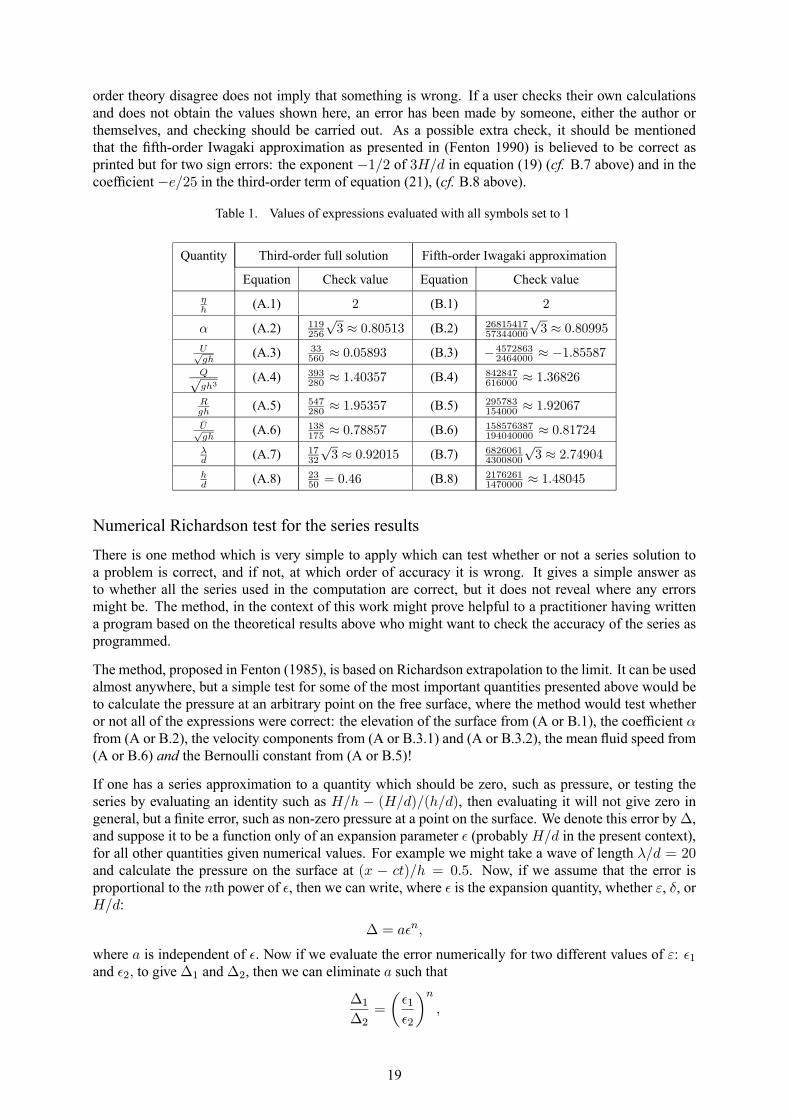
Table 1. Values of expressions evaluated with all symbols set to 1
Quantity Third-order full solution Fifth-order Iwagaki approximation
Equation Check value Equation Check valueηh (A.1) 2 (B.1) 2
There is one method which is very simple to apply which can test whether or not a series solution toa problem is correct, and if not, at which order of accuracy it is wrong. It gives a simple answer asto whether all the series used in the computation are correct, but it does not reveal where any errorsmight be. The method, in the context of this work might prove helpful to a practitioner having writtena program based on the theoretical results above who might want to check the accuracy of the series asprogrammed.
The method, proposed in Fenton (1985), is based on Richardson extrapolation to the limit. It can be usedalmost anywhere, but a simple test for some of the most important quantities presented above would beto calculate the pressure at an arbitrary point on the free surface, where the method would test whetheror not all of the expressions were correct: the elevation of the surface from (A or B.1), the coefficient αfrom (A or B.2), the velocity components from (A or B.3.1) and (A or B.3.2), the mean fluid speed from(A or B.6) and the Bernoulli constant from (A or B.5)!
If one has a series approximation to a quantity which should be zero, such as pressure, or testing theseries by evaluating an identity such as H/h − (H/d)/(h/d), then evaluating it will not give zero ingeneral, but a finite error, such as non-zero pressure at a point on the surface. We denote this error by∆,and suppose it to be a function only of an expansion parameter ² (probablyH/d in the present context),for all other quantities given numerical values. For example we might take a wave of length λ/d = 20and calculate the pressure on the surface at (x − ct)/h = 0.5. Now, if we assume that the error isproportional to the nth power of ², then we can write, where ² is the expansion quantity, whether ε, δ, orH/d:
∆ = a²n,
where a is independent of ². Now if we evaluate the error numerically for two different values of ε: ²1and ²2, to give∆1 and∆2, then we can eliminate a such that
∆1∆2
=
µ²1²2
¶n,
19
and this can be solved to give
n =log (∆1/∆2)
log (²1/²2), (39)
thus giving a numerical estimate of the error. The error of this expression can be shown to be O(²), soto provide convincing evidence of the order of the theory it is necessary to use a small value of ². Inpractice it is very reassuring to obtain a value of n = 5.98, for example, providing strong evidence thatall series that have gone into the calculation are correct to fifth order.
Formulae and methods for elliptic integrals and functionsElementary properties of elliptic functions and integrals
For elementary properties, reference can be made to Abramowitz & Stegun (1965), Gradshteyn &Ryzhik (1965) and Spanier & Oldham (1987), for example. Those sources contain a number of ap-proximations, but the expressions given usually do not have the same remarkable accuracy as thosegiven in Fenton & Gardiner-Garden (1982) for the limit required for cnoidal theory of waves, m → 1.If a reader were interested enough to investigate the theory, Eagle (1958) contains a refreshing differ-ent approach to the subject which inspired the work described below, originally obtained in Fenton &Gardiner-Garden (1982).
Approximations to functions and integrals
One perceived practical problem with the application of cnoidal theory has been that the theory makesuse of Jacobian elliptic functions and integrals, seen as being difficult to calculate. This has some justi-fication, as conventional formulae such as in Abramowitz & Stegun (1965) are very poorly convergent,if convergent at all, in the limit m→ 1, precisely the limit in which cnoidal theory is most appropriate.However, alternative formulae can be obtained which are most accurate and remarkably quickly conver-gent in the limit of m → 1. This has been done in (Fenton & Gardiner-Garden 1982), which providea number of useful expressions for both elliptic functions and integrals. The formulae are dramaticallyconvergent, even for values of m not in the m→ 1 limit. Convenient approximations to these formulaecan be obtained and are given here in Table 2. For values of m likely to be encountered using cnoidalwave theory the formulae are probably accurate to machine accuracy. It is remarkable that even form = 1/2, the simple approximations given in the table are accurate to five significant figures. For thecasem < 1/2, when cnoidal theory becomes less valid, conventional approximations could be used, forwhich reference can be made to Fenton & Gardiner-Garden (1982) or to standard references. However,cnoidal theory should probably be avoided in this case.
Although not necessary for the application of the above theory, there is an apparently little-knownFourier series for the cn2 function which might prove useful in certain applications. It is presentedhere, partly because in some fundamental references – (#911.01 of Byrd & Friedman 1954), (#8.146,
20
Table 2. Approximations for elliptic functions and integrals in the case most appro-priate for cnoidal theory,m ≥ 1/2.
Elliptic integralsComplete elliptic integral of the first kindK(m)
K(m) ≈ 2
(1+m1/4)2 log
2(1+m1/4)1−m1/4
Complementary elliptic integral of the first kindK0(m)K0(m) ≈ 2π
(1+m1/4)2
Complete elliptic integral of the second kind E(m)E(m) = K(m) e(m), where
e(m) ≈ 2−m3 + π
2KK0 + 2¡πK0¢2µ− 1
24 +q21
(1−q21)2
¶,
where q1(m) is the complementary nome q1 = e−πK/K0.
Jacobian elliptic functionssn(z|m) ≈ m−1/4 sinhw−q21 sinh 3w
coshw+q21 cosh 3w,
cn(z|m) ≈ 12
³m1
mq1
´1/41−2q1 cosh 2w
coshw+q21 cosh 3w,
dn(z|m) ≈ 12
³m1
q1
´1/41+2q1 cosh 2w
coshw+q21 cosh 3w,
in which w = πz/2K0.
26 of Gradshteyn & Ryzhik 1965) – an incorrect expression (an odd function) is given. The correctexpression is given in #2.23 of(Oberhettinger 1973) as a Fourier series for dn2() which can be used toconvert to a Fourier Series for cn2(), which can be written
cn2 (θ|m) = 1 + e− 1m
+π2
mK2
∞Xj=1
j
sinh (jπK 0/K)cos
µjπθ
K
¶. (42)
For typical shallow water waves,m→ 1, andK →∞, such that the series would be slowly convergent,as would be expected for a wave which is so non-sinusoidal as a long wave with its long trough andshort crest. The series could be re-cast to give a complementary rapidly-convergent formula whichwould involve a series of hyperbolic functions.
Convergence enhancement of series
The series above have been presented to third order for the full theory and to fifth order for the Iwagakiapproximation. There are several techniques available for obtaining more accurate results by taking theseries results and attempting to extract more information from the series than is apparently there.
The Shanks transform
One simple way of doing this is to use Shanks transforms, which are delightfully introduced in Shanks(1955), and used in the context of water wave theory to enhance the convergence of series in Fenton(1972). They take the first few terms of a series and attempt to mimic the behaviour of the series asif it had an infinite number of terms. The method takes three successive terms in a sequence (such asthe first, second and third order solutions for a wave property), and extrapolates the behaviour of thesequence to infinity, hopefully mimicking the behaviour of the series if there were an infinite number ofterms. There is little theoretical justification for the procedure, but it can work surprisingly well. It iseasily implemented: if the last three terms in a sequence of n terms are Sn−2, Sn−1, and Sn, an estimateof the value of S∞ is given by
This is not the form which is usually presented, but it is that which is most suitable for computations,when in the possible case that the sums have nearly converged and both numerator and denominator of
21
the second term on the right go to zero the result is less liable to round-off error. The transform doesindeed possess some remarkable properties. For example, it gives the exact sum to infinity for geometricseries, which can be verified by substituting Sn =
Pnj=0 r
j , then equation (43) gives 1/ (1− r), theexact result for the sum to infinity.
The transform is simply applied and can be used in many areas of numerical computations. It givessurprisingly good results, but its theoretical justification is limited and sometimes it does not work well.
Padé approximants
A form of approximation of the series which has more justification is that of Padé approximation, wherea rational function of the expansion variable is chosen such as to match the series expansion as muchas possible, Baker (1975), which was introduced to water wave theory by Schwartz (1974). The cal-culations for Padé approximants are not as trivial as for Shanks transforms, however the properties areusually more powerful. The [i, j] Padé approximation is defined to be the rational function p(²)/q(²),where p(²) is a polynomial of degree ≤ m and q(²) is a polynomial of degree ≤ n, such that the se-ries expansion of p(²)/q(²) has maximal initial agreement with the series expansion of the function. Innormal cases, the series expansion agrees through the term of degree m + n, and it is this way that thecoefficients in the two polynomials are computed. An example is (1 + x/2)/(1− x/2) as the [1, 1] ap-proximation to ex, which for small values of x is more accurate than the equivalent series with quadraticterms 1 + x + x2/2. Another example is where the function 1 + x + x2 has as its [1, 1] approximantthe function 1/ (1− x), and this too has ascertained that the first three terms of the series look like ageometric series.
Use of convergence acceleration procedures in cnoidal theory
The author has tested the use of both Shanks transforms and Padé approximants in applying the cnoidaltheory described in this work. As Padé approximation is considered more powerful, some attention wasgiven to that, however, a limitation became quickly obvious, when at the first step in application, solvingequation (B.7) for the wavelength, approximating the quartic in H/d in the large brackets by a [2, 2]Padé approximant, with a quadratic in numerator and denominator, the latter passed through zero foran intermediate value of H/d, such that in the vicinity of that point very wildly varying results wereobtained. The author considered that this was sufficiently dangerous that generally [2, 2] or [3, 2] Padéapproximants could not be recommended for the approximation of fifth-order cnoidal theory. Whenhe examined Padé approximants with a linear function in the denominator, it was found that, given ann-term series, the [n− 1, 1] Padé approximant is, in fact, exactly equal to the Shanks transform of thelast three sums in the series, as given in the equations above. As the Shanks transform is more simplyimplemented, we will refer to the series convergence acceleration using this method by that name.
In practice, obtaining solutions for given values of wavelength and wave height, the use of the Shankstransforms everywhere gave better results than just using the raw series in the case of global wavequantities such asα, Q, etc. which are independent of position, and it is recommended that for both third-order theory and the Iwagaki approximation that Shanks transforms be used to improve the accuracy ofall series computations for those quantities. They are of course trivially implemented, given say, threenumbers for the third, fourth and fifth solutions.
For the surface elevation and the fluid velocity components, however, because they are functions of po-sition, then depending on that position the series could show rather irregular behaviour, and it was foundthat the Shanks transform results could also be irregular. As in Fenton (1990), it is then recommendedthat for quantities which are functions of position, that no attempts be made to improve the accuracyby numerical transforming of the results, but that for all other quantities, characteristic of the wave asa whole, the Shanks transform be applied to all numerical evaluations of series. This procedure wasadopted for all the results shown further below.
22
A numerical cnoidal theory
Introduction
In Fenton (1990) the accuracies of various theories were examined by comparison with experimentalresults and with results from high-order numerical methods. It was found that fifth-order Stokes andcnoidal theory were of acceptable engineering accuracy almost everywhere within the range of validityof each. For long waves which are very high however, even the high-order cnoidal theory presentedabove becomes inaccurate. In such cases the most accurate method is to use a numerical method. Theusual method, suggested by the basic form of the Stokes solution, is to use a Fourier series which iscapable of accurately approximating any periodic quantity, provided the coefficients in that series can befound. A reasonable procedure, then, instead of assuming perturbation expansions for the coefficientsin the series as is done in Stokes theory, is to calculate the coefficients numerically by solving the fullnonlinear equations. This approach began with Chappelear (1961), and has been often but inappropri-ately known as ”stream function theory” (Dean 1965). Further developments include those of Rienecker& Fenton (1981). A comparison of the various methods has been given in Sobey et al. (1987), wherethe conclusion was drawn that there was little to choose between them. A more recent development hasbeen the simpler method and computer program given in Fenton (1988).
This Fourier approach breaks down in the limit of very long waves, when the spectrum of coefficientsbecomes broad-banded and many terms have to be taken, as the Fourier approximation has to approx-imate both the short rapidly-varying crest region and the long trough where very little changes. Moreof a problem is that it is difficult to get the method to converge to the solution desired, (Dalrymple &Solana 1986).
A new approach was suggested in Fenton (1995), which describes a numerical cnoidal theory, which isto cnoidal theory what the various Fourier approximation methods are to Stokes theory, in that it solvesthe problem numerically by assuming series of cnoidal-type functions, but rather than solving them byanalytical power series methods as above, the coefficients in the equations are found numerically andthere is no essential mathematical approximation introduced. The method will be described here briefly.
Theory
A spectral approach is used, in which all functions of x are approximated by polynomials of degree Nin terms of the square of the Jacobian elliptic function cn2(θ|m) for the surface elevation and bottomvelocity of the form suggested by conventional cnoidal theory:
η∗ = 1 +NXj=1
Yj cn2j (θ|m) , (44)
f 0∗ = F0 +NXj=1
Fj cn2j (θ|m) , (45)
where the Yj and Fj are numerical coefficients for a particular wave. Note that theN here is not the orderof approximation but the number of terms in the series. Conventional cnoidal theory expresses the coeffi-cients as expansions in terms of the parameter αwhich is related to the shallowness (depth/wavelength)2,equations (14) and (15), and produces a hierarchy of equations and solutions based on series expansionsin terms of α, which is required to be small. In this work there is no attempt to solve the equations bymaking expansions in terms of physical quantities. The surface velocity components are then given by
u∗s =ush
Q= − cosαη∗
d
dθ. f 0∗,
v∗s =vsh
Q= sinαη∗
d
dθ. f 0∗. (46)
On substituting these into the nonlinear surface boundary conditions, equations (12) and (13) we have
23
two nonlinear algebraic equations valid for all values of θ. The equations include the following un-knowns: α, m, g∗, R∗, plus a total of N values of the Yj for i = 1 . . . N , and N + 1 values of the Fjfor i = 0 . . . N , making a total of 2N + 5 unknowns. For the boundary points at which both boundaryconditions are to be satisfied we choose M + 1 points equally spaced in the vertical between crest andtrough such that:
cn2 (θi|m) = 1− i/M, for i = 0 . . .M, (47)
where i = 0 corresponds to the crest and i = M to the trough. This has the effect of clustering pointsnear the wave crest, where variation is more rapid and the conditions at each point will be relativelydifferent from each other. If we had spaced uniformly in the horizontal, in the long trough where condi-tions vary little the equations obtained would be similar to each other and the system would be poorlyconditioned. We now have a total of 2M + 2 equations but so far, none of the overall wave parametershave been introduced. It is known that the steady wave problem is uniquely defined by two dimension-less quantities: the wavelength λ/d and the wave height H/d. In many practical problems the waveperiod is known, but Fenton (1995) considered only those where the dimensionless wavelength λ/d isknown. It can be shown that λ/d is related to α using the expression (24) which we term the WavelengthEquation:
αλ
d
d
h− 2K(m) = 0, (48)
where K(m) is the complete elliptic integral of the first kind, and where the equation has introducedanother unknown d/h, the ratio of mean to trough depth.
The equation for this ratio is obtained by taking the mean of equation (44) over one wavelength or halfa wavelength from crest to trough:
d
h= 1 +
NXj=1
Yj cn2j (θ|m). (49)
The mean values of the powers of the cn function over a wavelength can be computed from the recur-rence relations (26) for the Ij such that equation (49) can be written
1 +NXj=1
Yj Ij − dh= 0, (50)
thereby providing one more equation, the Mean Depth Equation.
Finally, another equation which can be used is that for the wave height:
H
h=
η0h− ηM
h, (51)
which, on substitution of equation (44) at x = x0 = 0 where cn(0|m) = 1 and, because cn(αxM |m) =0 from equation (47), gives
H
d
d
h−
NXj=1
Yj = 0, (52)
the Wave Height Equation.
We write the system of equations as
e (z) = {ei (z) , i = 1 . . . 2M + 5} = 0, (53)
where ei is the equation with reference number i, the 2M + 2 equations described above plus the threeequations (48), (50), and (52), and where the variables which are used are the 2N+5 unknowns describedabove plus d/h:
z = {zj , j = 1 . . . 2N + 6} , (54)
24
Whereas the parameter m has been used in cnoidal theory, it has the unpleasant property that it has asingularity in the limit as m → 1, which corresponds to the long wave limit, and as we will be usinggradient methods to solve the nonlinear equations this might make solution more difficult. It is moreconvenient to use the ratio of the complete elliptic integrals as the actual unknown, which we choose tobe the first:
z1 =K(m)
K(1−m) . (55)
The solution of the system of nonlinear equations follows that in Fenton (1988), using Newton’s methodin a number of dimensions, where it is simpler to obtain the derivatives by numerical differentiation.
As the number of equations and variables can never be the same (2M + 5 can never equal 2N + 6 forinteger M and N ), we have to solve this equation as a generalised inverse problem. Fortunately thiscan be done very conveniently by the Singular Value Decomposition method (for example #2.6 of Press,Teukolsky, Vetterling & Flannery 1992) so that if there are more equations than unknowns, M > N ,the method obtains the least squares solution to the overdetermined system of equations. In practice thiswas found to give a certain rugged robustness to the method, despite the equations being rather poorlyconditioned.
form an orthogonal set, and they all tend to look like one another, which result, although apparently anesoteric mathematical property, has the important effect that the system of equations is not particularlywell-conditioned, and numerical solutions show certain irregularities and a relatively slow convergencewith the number of terms taken in the series. It was difficult to obtain solutions for N > 10. TheFourier methods, however, using the robustly orthogonal trigonometric functions, do not seem to havethese problems. Fortunately, however, in the case of the numerical cnoidal theory, good results could beobtained with few terms.
For initial conditions in the iteration process, it was obvious to choose the fifth order Iwagaki theorypresented in equations (B.1-B.8). The first step is to compute an approximate value of m and hence z1using the analytical expression for wavelength in terms of m from equation (B.7), combined with thebisection method of finding the root of a single transcendental equation. After that the rest of the fifthorder expressions presented above can be used.
Accuracy of the methods
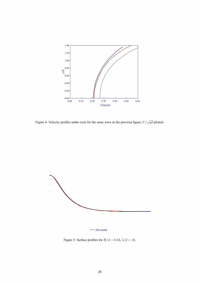
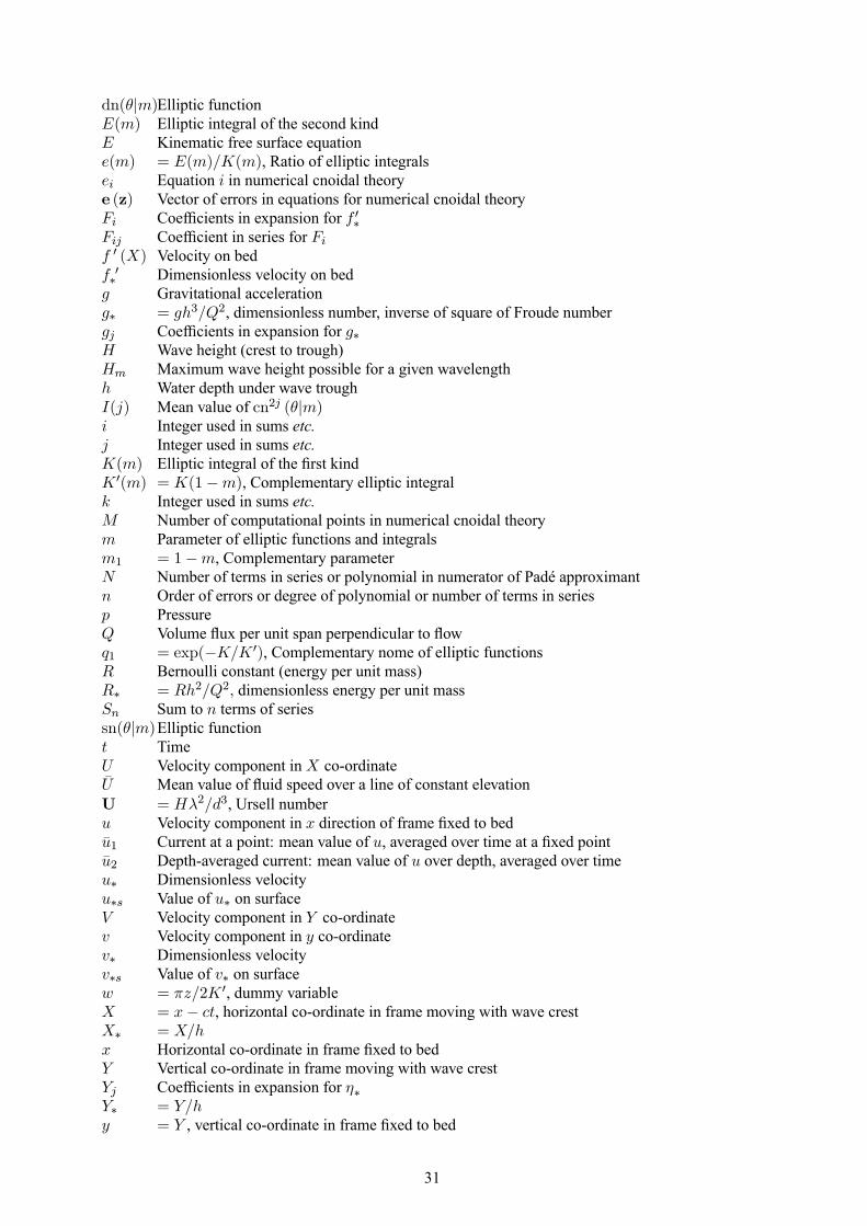
In this section we examine the applicability of the full third-order cnoidal theory, the fifth-order Iwagakiapproximation and the numerical cnoidal theory by considering several high waves and showing resultsfor the surface profile and possibly more importantly, for the velocity profile under the crest.
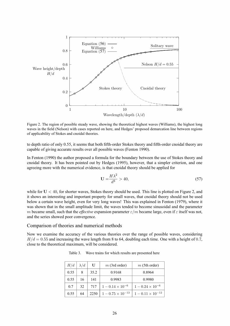
The region of possible waves and the validity of theories
The range over which periodic solutions for waves can occur is given in Figure 2, which shows limitsto the existence of waves determined by computational studies. The highest waves possible, H = Hm,are shown by the thick line, which is the approximation to the results of Williams (1981), presented asequation (32) in Fenton (1990) :
Hmd=
0.141063 λd + 0.0095721
¡λd
¢2+ 0.0077829
¡λd
¢31 + 0.0788340 λ
d + 0.0317567¡λd
¢2+ 0.0093407
¡λd
¢3 . (56)
Nelson (1987, ) has shown from many experiments in laboratories and the field, that the maximum waveheight achievable in practice is actually only Hm/d = 0.55. Further evidence for this conclusion isprovided by the results of Le Méhauté et al. (1968), whose maximum wave height tested was H/d =0.548, described as ”just below breaking”. It seems that there may be enough instabilities at work thatreal waves propagating over a flat bed cannot approach the theoretical limit given by equation (56). Thisis fundamental for the application of the present theories. If indeed the highest waves do have a height
25
0
0.2
0.4
0.6
0.8
1
1 10 100
Wave height/depth
H/d
Wavelength/depth (λ/d)
Solitary wave
Nelson H/d = 0.55
Stokes theory Cnoidal theory
Equation (56)Williams cccccccccccccccccccc
cEquation (57)
Figure 2. The region of possible steady wave, showing the theoretical highest waves (Williams), the highest longwaves in the field (Nelson) with cases reported on here, and Hedges’ proposed demarcation line between regionsof applicability of Stokes and cnoidal theories.
to depth ratio of only 0.55, it seems that both fifth-order Stokes theory and fifth-order cnoidal theory arecapable of giving accurate results over all possible waves (Fenton 1990).
In Fenton (1990) the author proposed a formula for the boundary between the use of Stokes theory andcnoidal theory. It has been pointed out by Hedges (1995), however, that a simpler criterion, and oneagreeing more with the numerical evidence, is that cnoidal theory should be applied for
U =Hλ2
d3> 40, (57)
while forU < 40, for shorter waves, Stokes theory should be used. This line is plotted on Figure 2, andit shows an interesting and important property for small waves, that cnoidal theory should not be usedbelow a certain wave height, even for very long waves! This was explained in Fenton (1979), where itwas shown that in the small amplitude limit, the waves tended to become sinusoidal and the parameterm became small, such that the effective expansion parameter ε/m became large, even if ε itself was not,and the series showed poor convergence.
Comparison of theories and numerical methods
Now we examine the accuracy of the various theories over the range of possible waves, consideringH/d = 0.55 and increasing the wave length from 8 to 64, doubling each time. One with a height of 0.7,close to the theoretical maximum, will be considered.
Table 3. Wave trains for which results are presented here
H/d λ/d U m (3rd order) m (5th order)
0.55 8 35.2 0.9168 0.8964
0.55 16 141 0.9983 0.9980
0.7 32 717 1− 0.14× 10⁻⁶ 1− 0.24× 10⁻⁶
0.55 64 2250 1− 0.75× 10⁻¹³ 1− 0.11× 10⁻¹²
26
These cases are summarised in Table 3, which shows the wave dimensions, the Ursell number, and thevalue ofm obtained by solving equation (B.7).
Figure 3 shows the solution for the surface profiles obtained for a high wave of intermediate length,when conventional cnoidal theory has been considered not valid, and which falls outside Hedges’ rec-ommended boundary for cnoidal theory ofU ≥ 40, as can be seen on Figure 2. Four curves are plotted,results from the full third-order method, the fifth-order Iwagaki approximation (shown as m~ 1), thenumerical cnoidal theory described above, and from the Fourier approximation method, which shouldbe highly accurate in this relatively short wave limit. It can be seen that most results are almost indis-tinguishable at the scale of plotting, but that in this case of a relatively short wave, with m ≈ 0.9, theIwagaki approximation is not so accurate, as expected. Whereas conventional cnoidal theory shouldnot be particularly accurate in this shorter wave limit, as it depends on the waves being long for itsaccuracy, there is nothing in the numerical cnoidal method which necessarily limits its accuracy to longwaves. In fact, for the initial conditions for the numerical method only cnoidal theory was used, andit was not accurate enough for waves shorter than this example. If Stokes theory could be modified toprovide the initial conditions, there is no reason why the numerical cnoidal method could not be usedfor considerably shorter waves.
Figure 4 shows the velocity profiles under the crest for the same wave. It is clear that the numericalcnoidal method and the Fourier method agree closely, and possibly strangely, that the Iwagaki approx-imation is accurate, even for this wave with m ≈ 0.9. The third-order theory predicts the mean fluidspeed under the wave poorly, but predicts the velocity variation in the vertical very well, so that the curveis displaced relative to the accurate results.
Figure 5 shows the results for a longer wave, of λ/d = 16. In this case, m = 0.998, and it is expectedthat the Iwagaki approximation would be accurate. It can be seen that even the third-order theory predictsthe surface very accurately. For all subsequent cases studied, even for the higher wave withH/d = 0.7,the results for surface elevation were better even than this, and no more results for surface elevation willbe presented here.
Figure 6 shows the velocity profiles under the crest. It is clear that the fifth-order Iwagaki theory ishighly accurate for practical purposes, but that the third-order theory has a constant shift as before.
Figure 7 shows the behaviour of the numerical cnoidal method for very high and long waves, for awave of length λ/d = 32 and a height of H/d = 0.7, close to the maximum theoretical height ofHm/d = 0.737, calculated from equation (56). There is evidence that no long wave in shallow watercan exist at this height, and that a maximum of H/d = 0.55 is more likely (Nelson 1994). This waveis sufficiently long that the Fourier method is beginning to be tested considerably, yet it is capable of
27
0.00
0.20
0.40
0.60
0.80
1.00
1.20
1.40
y/d
0.00 0.10 0.20 0.30 0.40 0.50 0.60 Velocity
Figure 4. Velocity profiles under crest for the same wave as the previous figure; U/√gd plotted.
Figure 7. Velocity profiles under crest for high and long wave: H/d = 0.7, λ/d = 32.
29
giving results provided sufficient numbers of Fourier terms are taken and sufficient steps in wave heightare taken. It can be seen that the present numerical cnoidal theory is also capable of high accuracy,as demonstrated by the close agreement between the two very different theories. It used much smallercomputing resources, typically using 9-10 spectral terms with the solution of systems of 25 equationscompared with the Fourier method with some 25 spectral terms and some 70 equations. However, it canbe seen that there are some irregularities in the solution, and the results for different values of N do notagree to within plotting accuracy. Although the method shows difficulty with convergence, it does yieldresults of engineering accuracy. It is still remarkable, however, that such a demanding problem can besolved with so few ”spectral terms”.
Figure 8 shows the velocity profile under the crest for a very long wave, λ/d = 64, with Nelson’smaximum heightH/d = 0.55. The Fourier method took a large number of steps to converge that it wasconsidered not worth while. The numerical cnoidal method performed quite well, although there wassome variation between the solutions for N = 5 to N = 9. What is noteworthy, however, is that thefifth-order Iwagaki theory gave a good engineering accuracy solution to this problem.
Conclusions from computational results
The numerical cnoidal method has been shown to be accurate for waves longer than some eight times thewater depth. It can treat very long waves rather more easily than Fourier methods can. As the theoreticalhighest waves are approached, however, the accuracy decreases to an approximate engineering accuracy.However there is strong evidence that these waves cannot be achieved in practice. Throughout, however,for waves with an Ursell number greater than 40, and apparently even for high waves, the fifth-orderIwagaki theory presented in this work gave satisfactory engineering solutions to the problems studied.
List of Symbols
Symbol DefinitionRoman symbolsa Constant in numerical test of order of accuracyc Wave speedcn(θ|m)Elliptic functionD(²) polynomial in denominator of Padé approximantd Mean water depth
30
dn(θ|m)Elliptic functionE(m) Elliptic integral of the second kindE Kinematic free surface equatione(m) = E(m)/K(m), Ratio of elliptic integralsei Equation i in numerical cnoidal theorye (z) Vector of errors in equations for numerical cnoidal theoryFi Coefficients in expansion for f 0∗Fij Coefficient in series for Fif 0 (X) Velocity on bedf 0∗ Dimensionless velocity on bedg Gravitational accelerationg∗ = gh3/Q2, dimensionless number, inverse of square of Froude numbergj Coefficients in expansion for g∗H Wave height (crest to trough)Hm Maximum wave height possible for a given wavelengthh Water depth under wave troughI(j) Mean value of cn2j (θ|m)i Integer used in sums etc.j Integer used in sums etc.K(m) Elliptic integral of the first kindK 0(m) = K(1−m), Complementary elliptic integralk Integer used in sums etc.M Number of computational points in numerical cnoidal theorym Parameter of elliptic functions and integralsm1 = 1−m, Complementary parameterN Number of terms in series or polynomial in numerator of Padé approximantn Order of errors or degree of polynomial or number of terms in seriesp PressureQ Volume flux per unit span perpendicular to flowq1 = exp(−K/K 0), Complementary nome of elliptic functionsR Bernoulli constant (energy per unit mass)R∗ = Rh2/Q2, dimensionless energy per unit massSn Sum to n terms of seriessn(θ|m)Elliptic functiont TimeU Velocity component inX co-ordinateU Mean value of fluid speed over a line of constant elevationU = Hλ2/d3, Ursell numberu Velocity component in x direction of frame fixed to bedu1 Current at a point: mean value of u, averaged over time at a fixed pointu2 Depth-averaged current: mean value of u over depth, averaged over timeu∗ Dimensionless velocityu∗s Value of u∗ on surfaceV Velocity component in Y co-ordinatev Velocity component in y co-ordinatev∗ Dimensionless velocityv∗s Value of v∗ on surfacew = πz/2K 0, dummy variableX = x− ct, horizontal co-ordinate in frame moving with wave crestX∗ = X/hx Horizontal co-ordinate in frame fixed to bedY Vertical co-ordinate in frame moving with wave crestYj Coefficients in expansion for η∗Y∗ = Y/hy = Y , vertical co-ordinate in frame fixed to bed
31
z Dummy argument used in elliptic function formulaezj Variable j in numerical cnoidal theory, z1 = K(m)/K(1−m)z = {zj , j = 1 . . . 2M + 6}, vector of variablesGreek symbolsα Coefficient ofX/h in elliptic functions and expression of shallowness∆ Error in any equationδ = 4
3α2, quantity used in series for velocity components
² general symbol for expansion quantity of series: ε, δ orH/dε = H/h, dimensionless wave heightη Water depthη∗ = η/h, dimensionless water depthθ Argument of elliptic functions, often αX/h in this workλ Wavelengthρ Fluid densityτ Wave periodΦijl Velocity coefficients in cnoidal theoryψ Stream functionψ∗ = ψ ×
pgh3/Q, dimensionless stream function
Mathematical symbolsO() Order symbol: ”neglected terms are at least of the order of”[i, j] Padé approximant with ith and jth degree polynomials in numerator and denominator
References
Abramowitz, M. & Stegun, I. A. (1965) Handbook of Mathematical Functions, Dover, New York.
Baker, G. A. (1975) Essentials of Padé Approximants, Academic.
Benjamin, T. B. & Lighthill, M. J. (1954) On cnoidal waves and bores, Proc. Roy. Soc. Lond. A224, 448–460.
Boussinesq, J. (1871) Théorie de l’intumesence liquide appelée onde solitaire ou de translation, sepropageant dans un canal rectangulaire, Comptes Rendus Acad. Sci., Paris 72, 755–759.
Byrd, P. F. & Friedman, M. D. (1954) Handbook of Elliptic Integrals for Engineers and Physicists,Springer, Berlin.
Chappelear, J. E. (1961) Direct numerical calculation of wave properties, J. Geophys. Res. 66, 501–508.
Chappelear, J. E. (1962) Shallow-water waves, J. Geophys. Res. 67, 4693–4704.
Conte, S. D. & de Boor, C. (1980) Elementary Numerical Analysis,(Third edn.), McGaw-Hill Ko-gakusha, Tokyo.
Dalrymple, R. A. & Solana, P. (1986) Nonuniqueness in stream function wave theory, J. Waterway PortCoastal and Ocean Engng 112, 333–337.
Dean, R. G. (1965) Stream function representation of nonlinear ocean waves, J. Geophys. Res. 70, 4561–4572.
Eagle, A. (1958) The Elliptic Functions as they should be, Galloway & Porter, Cambridge.
Fenton, J. D. (1972) A ninth-order solution for the solitary wave, J. Fluid Mech. 53, 257–271.
Fenton, J. D. (1979) A high-order cnoidal wave theory, J. Fluid Mech. 94, 129–161.
Fenton, J. D. (1985) A fifth-order Stokes theory for steady waves, J. Waterway Port Coastal and OceanEngng 111, 216–234.
Fenton, J. D. (1988) The numerical solution of steady water wave problems, Computers and Geo-sciences 14, 357–368.
Fenton, J. D. (1990) Nonlinear wave theories, The Sea - Ocean Engineering Science, Part A, B. Le
32
Méhauté & D. M. Hanes (eds), Vol. 9, Wiley, New York, pp. 3–25.
Fenton, J. D. (1995) A numerical cnoidal theory for steady water waves, in Proc. 12th AustralasianCoastal and Ocean Engng Conference, Melbourne, pp. 157–162.
Fenton, J. D. & Gardiner-Garden, R. S. (1982) Rapidly-convergent methods for evaluating ellipticintegrals and theta and elliptic functions, J. Austral. Math. Soc. Ser. B 24, 47–58.
Gradshteyn, I. S. & Ryzhik, I. M. (1965) Table of Integrals, Series, and Products, Fourth Edn, Acad-emic.
Hedges, T. S. (1978) Some effects of currents on measurement and analysis of waves, Proc. Inst. Civ.Engrs. 65, 685–692.
Hedges, T. S. (1995) Regions of validity of analytical wave theories, Proc. Inst. Civ. Engnrs, Water,Maritime and Energy 112, 111–114.
Isobe, M., Nishimura, H. & Horikawa, K. (1982) Theoretical considerations on perturbation solutionsfor waves of permanent type, Bull. Faculty of Engng, Yokohama National University 31, 29–57.
Iwagaki, Y. (1968) Hyperbolic waves and their shoaling, in Proc. 11th Int. Conf. Coastal Engng, Lon-don, Vol. 1, pp. 124–144.
Jonsson, I. G., Skougaard, C. & Wang, J. D. (1970) Interaction between waves and currents, in Proc.12th Int. Conf. Coastal Engng, Washington D.C., Vol. 1, pp. 489–507.
Keller, J. B. (1948) The solitary wave and periodic waves in shallow water, Comm. Appl. Math. 1, 323–339.
Keulegan, G. H. & Patterson, G. W. (1940) Mathematical theory of irrotational translation waves, J.Res. Nat. Bur. Standards 24, 47–101.
Korteweg, D. J. & de Vries, G. (1895) On the change of form of long waves advancing in a rectangularcanal, and on a new type of long stationary waves, Phil. Mag. (5) 39, 422–443.
Laitone, E. V. (1960) The second approximation to cnoidal and solitary waves, J. Fluid Mech. 9, 430–444.
Laitone, E. V. (1962) Limiting conditions for cnoidal and Stokes waves, J. Geophys. Res. 67, 1555–1564.
Le Méhauté, B., Divoky, D. & Lin, A. (1968) Shallow water waves: a comparison of theories andexperiments, in Proc. 11th Int. Conf. Coastal Engng, London, Vol. 1, pp. 86–107.
Nelson, R. C. (1987) Design wave heights on very mild slopes - an experimental study, Civ. EngngTrans, Inst. Engnrs Austral. CE29, 157–161.
Nelson, R. C. (1994) Depth limited design wave heights in very flat regions, Coastal Engng 23, 43–59.
Nishimura, H., Isobe, M. & Horikawa, K. (1977) Higher order solutions of the Stokes and the cnoidalwaves, J. Faculty of Engng, The University of Tokyo 34, 267–293.
Oberhettinger, F. (1973) Fourier Expansions, Academic, New York & London.
Poulin, S. & Jonsson, I. G. (1994) A simplified high-order cnoidal theory, in Proc. Int. Symp. on Waves- Physical and Numerical Modelling, Vancouver, Vol. 1, pp. 406–416.
Press, W. H., Teukolsky, S. A., Vetterling, W. T. & Flannery, B. P. (1992) Numerical Recipes in C,Second Edn, Cambridge.
Rayleigh, L. (1876) On waves, Phil. Mag. (5) 1, 257–279.
Rienecker, M. M. & Fenton, J. D. (1981) A Fourier approximation method for steady water waves, J.Fluid Mech. 104, 119–137.
Schwartz, L. W. (1974) Computer extension and analytical coninuation of Stokes’ expansion for gravitywaves, J. Fluid Mech. 65, 553–578.
Shanks, D. (1955) Non-linear transformations of divergent and slowly convergent sequences, J. Math.
33
Phys. 34, 1–42.
Shen, S. S. (1993) A Course on Nonlinear waves, Kluwer, Dordrecht.
Sobey, R. J., Goodwin, P., Thieke, R. J. & Westberg, R. J. (1987) Application of Stokes, cnoidal, andFourier wave theories, J. Waterway Port Coastal and Ocean Engng 113, 565–587.
Spanier, J. & Oldham, K. B. (1987) An Atlas of Functions, Hemisphere, Washington D.C.
Tsuchiya, Y. & Yasuda, T. (1985) Cnoidal waves in shallow water and their mass transport, Advancesin Nonlinear Waves, L. Debnath (ed.), Pitman, pp. 57–76.
Ursell, F. (1953) The long-wave paradox in the theory of gravity waves, Proc. Camb. Phil. Soc. 49, 685–694.
Wiegel, R. L. (1960) A presentation of cnoidal wave theory for practical application, J. Fluid Mech.7, 273–286.
Wiegel, R. L. (1964) Oceanographical Engineering, Prentice-Hall.
Williams, J. M. (1981) Limiting gravity waves in water of finite depth, Phil. Trans Roy. Soc. London A302, 139–188.