THE COMMUNITY MULTISCALE AIR QUALITY (CMAQ) MODEL:

Model Configuration and Enhancements for 2006 Air Quality Forecasting

Rohit Mathur, Jonathan Pleim, Kenneth Schere, George Pouliot, Jeffrey Young, Tanya OtteAtmospheric Sciences Modeling Division

ARL/NOAANERL/U.S. EPA

Hsin-Mu Lin, Daiwen Kang, Daniel Tong, Shaocai Yu, Science and Technology Corporation

DisclaimerDisclaimer: The research presented here was performed under the : The research presented here was performed under the Memorandum of Understanding between the U.S. Environmental Protection Memorandum of Understanding between the U.S. Environmental Protection Agency (EPA) and the U.S. Department of Commerce’s National Oceanic and Agency (EPA) and the U.S. Department of Commerce’s National Oceanic and Atmospheric Administration (NOAA) and under agreement number Atmospheric Administration (NOAA) and under agreement number DW13921548. This work constitutes a contribution to the NOAA Air Quality DW13921548. This work constitutes a contribution to the NOAA Air Quality Program. Although it has been reviewed by EPA and NOAA and approved for Program. Although it has been reviewed by EPA and NOAA and approved for publication, it does not necessarily reflect their views or policies.publication, it does not necessarily reflect their views or policies.

Acknowledgements

• Jeff McQueen, Pius Lee, Marina Tsidulko• Paula Davidson

Verification ToolsVerification Tools

CMAQCMAQ

WRF PostWRF Post

PRDGENPRDGEN

AQF PostAQF Post

Vertical interpolation

Horizontal interpolation to Lambert grid

CMAQ-ready meteorology and emissions

Gridded ozone files for users

Chemistry/Transport/Deposition model

NAM Meteorology model

Performance feedback for users/developers

PREMAQPREMAQ

Meteorological Observations

EmissionInventory Data

WRF-NMMWRF-NMM

Air Quality Observations

WRF-NMM-CMAQ AQF System

268 grid cells

259gridcells

East “3x” Domain

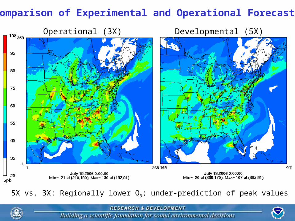
CMAQ Modeling DomainsOzone forecasts both domainsExperimental PM forecasts on 5x

12 km resolution

CONUS “5x” Domain Experimental

265gridcells

442 grid cells

Emission Processing

• Emission Processing is a component of PREMAQ (pre-processor to CMAQ)

Point Source and Biogenic Source processing from SMOKE

Area Sources (no meteorological modulation) computed in SMOKE outside of PREMAQ

Mobile Sources (nonlinear least squares approximation to SMOKE/Mobile6)

Area and Biogenic Sources

• Area Sources: Computed outside of PREMAQ 2001 NEI version 3 inventory used. (CAIR) No

changes made to inventory. Replaced year specific with average (1996-2002)

estimates for fires

• Biogenic Sources: BEIS3.13 included directly into PREMAQ.

• Canadian Inventory: 1995 used (includes all provinces)

• Mexican Inventory: BRAVO 1999 used for point sources

Mobile Sources

• SMOKE/MOBILE6 not efficient for real-time forecasting

• SMOKE/MOBILE6 used to create retrospective emissions for AQF grid 2006 (projected from 2001) VMT data used for input to

Mobile 6 2006 Vehicle Fleet used for input to Mobile 6

• For 13 counties in Metropolitan Atlanta area, VMT based on 2005 run of a travel demand model and Mobile6 inputs from Georgia DNR

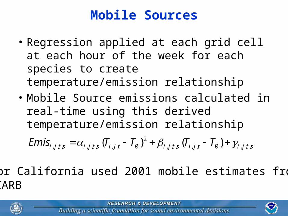
Mobile Sources

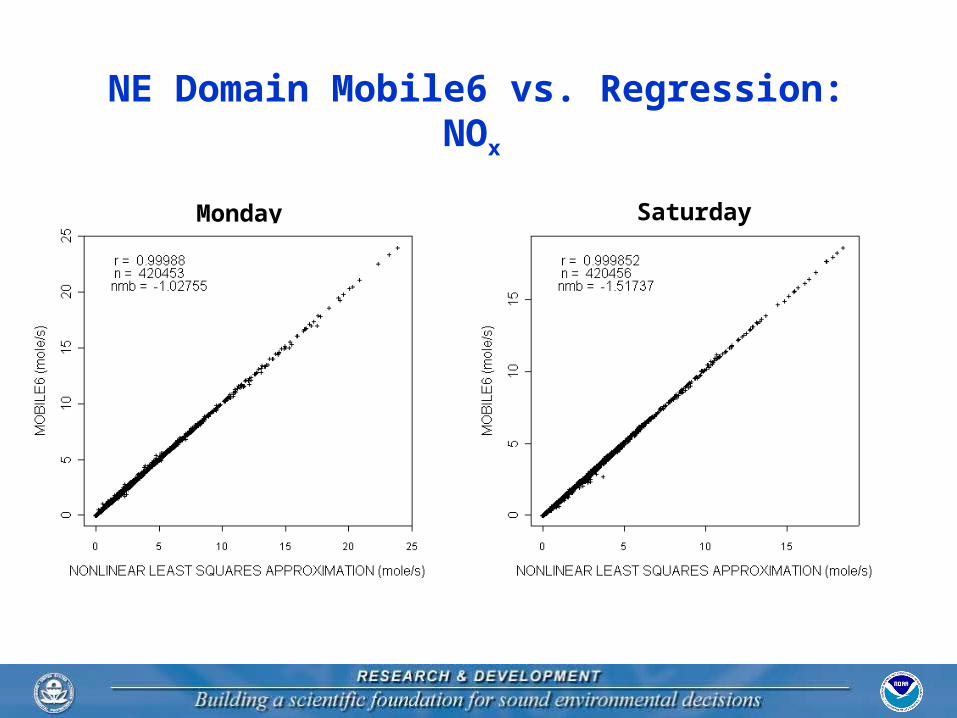
• Regression applied at each grid cell at each hour of the week for each species to create temperature/emission relationship

• Mobile Source emissions calculated in real-time using this derived temperature/emission relationship

stjitjistjitjistjistji TTTTEmis ,,,0,,,,,2

0,,,,,,,, )()(

• For California used 2001 mobile estimates from CARB

NE Domain Mobile6 vs. Regression: NOx

Monday Saturday

NE Domain Mobile6 vs. Regression: VOC

Monday Saturday

Point Sources

• 2004 Continuous Emissions Monitoring for NOx and SO2

Monthly temporal profiles on a state-by-state basis derived from 2004 CEM

• For other pollutants and non-EGU: 2001 NEIv3 Georgia non-EGU based on 2002 inventory from

GADNR

• Modified EGU NOx emissions using DOE’s Annual Energy Outlook (Jan. 2006)

• Calculated 2006/2004 NOx and SO2 annual emission ratios on a regional basis (from DOE data) Exception California

1.03

1.01

1.12

1.0

0.74

0.95

1.641.20

1.110.98

1.02

1.56

0.84

EGU NOX adjustments 2006/2004 by region

Source: Department of Energy Annual Energy Outlook 2006 http://www.eia.doe.gov/oiaf/aeo/index.html

DOE/AOE estimatedan increase by factor of 8

CMAQ Configuration

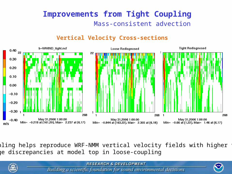
• Advection Horizontal: Piecewise Parabolic Method Vertical: Upstream with rediagnosed vertical velocity to satisfy

mass conservation

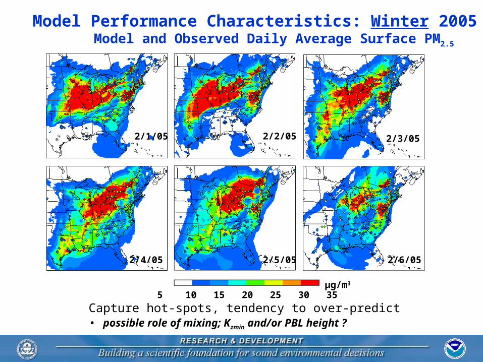
• Turbulent Mixing K-theory; PBL height from WRF-NMM Minimum value of Kz allowed to vary spatially depending on

urban fraction (furban)• Kz = 0.1 m2/s, furban = 0• Kz = 2.0 m2/s, furban = 1

allows min. Kz in rural areas to fall off to lower values than urban regions during night-time

prevents precursor concentrations (e.g., CO, NOx) in urban areas from becoming too large at night; reduced mixing intensity) in non-urban areas results in increased night-time O3 titration

CMAQ Configuration (contd.)

• Gas phase chemistry CB4 mechanism with EBI solver Below cloud attenuation based on ratio of radiation

reaching the surface to its clear-sky value• Closer linkage with the NAM fields

• Cloud Processes Mixing and aqueous chemistry Scavenging and wet deposition Sub-grid scheme based on modifications to RADM formulation;

“switch-off” entrainment from above clouds• Used in Eastern U.S. (3x) domain

“In-cloud” mixing based on the Asymmetric Convective Mixing (ACM) model (Pleim and Chang, 1992, JGR)

• Used in Continental U.S. (5x) domain

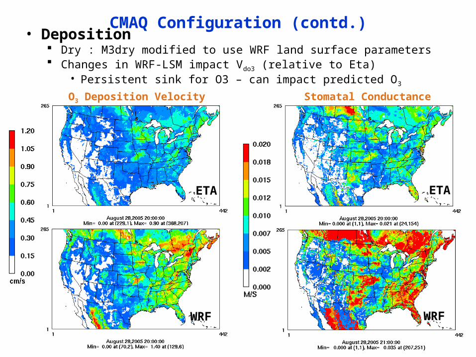
CMAQ Configuration (contd.)• Deposition

Dry : M3dry modified to use WRF land surface parameters Changes in WRF-LSM impact Vdo3 (relative to Eta)

• Persistent sink for O3 – can impact predicted O3

ETA

WRF

ETA

WRF

O3 Deposition Velocity Stomatal Conductance

NO3-

NH4+

SO4=

Na+

Cl-

H2O

POA

SOAa

SOAb

EC

Other

SVOCs

HNO3

NH3

H2O

Na+, Cl-, SO42-

Soil, Other

COARSE MODE2 FINE MODES

H2SO4

Aromatics

Monoterpenes

HCl

• Trimodal size distribution• Aitken (0-0.1 µm), Accumulation(0.1-2.5 µm), and Coarse

• Gas/particle interactions treated for fine modes only – ISORROPIA instantaneous equilibrium

• Fine-modes coagulate

• Coarse mode, fine EC (black) & other fine PM (brown) are inert

CMAQ Configuration: Aerosols

Binkowski and Roselle, JGR, 2002

Structural Enhancements

• Included layer dependent advection time-step calculation Improves model efficiency

• Coupling between WRF-NMM and CMAQ “Loose-coupling” (used in Operational 3X)

• Similar to previous Eta-CMAQ linkage • WRF-NMM and CMAQ coordinate and grid structures are

different. Interpolation of meteorological inputs to the CMAQ grid and coordinate

“Tight-coupling” (implemented in Experimental 5X)• Step 1: Coupling in the vertical implemented this summer

– CMAQ calculations on the same vertical coordinate as WRF-NMM

• Step 2: Modifications to CMAQ to facilitate calculations on native WRF-NMM horizontal grid

– Stay tuned

PD

PDT

PT

Ps = PD + PDT + PT

WRF-NMM Hybrid Vertical Coordinate System“Tightly Coupled”

2313

223113

21

3

213

21

21

2,

2

2

)1()1(

,)(

xx

JxJxJ

g

PDJ

g

PDJ

x

zJ

x

PD

PP

PD

PPDP

PPDPDP

h

T

T

TTT

TT

’s limited to 0-1

Jacobian across the interface

Jacobian: encapsulates coordinate transformations between physical and computational space

Tightly Coupled SystemConversion to use WRF-NMM vertical coordinate in PREMAQ and CMAQ

Comparison of Experimental and Operational Forecasts Mean over sites within Operational 3x Domain

5X under-predictions at peak values

Comparison of Experimental and Operational Forecasts

Operational (3X) Developmental (5X)

5X vs. 3X: Regionally lower O3; under-prediction of peak values

Diagnosing the low-bias in Experimental 5X Runs

Black (Loose), Red (Tight w/ISOP error), Green (Corrected Tight)

California Sub-domain average time series: July 18-19, 2006

Isoprene

NTR

Ozone

NTR: Inert organic nitrate in CBM-IV

Correcting the low-bias in Experimental 5X Runs

Loose Old Tight IsopreneFix Tight

Max.-8hr O3: 7/19/06

Correcting the low-bias in Experimental 5X Runs

Max. 8 O3 7/19/06

Loose

Old Tight

Isoprene Fix Tight

Improvements from Tight Coupling Mass-consistent advection

Vertical Velocity Cross-sections

Tight coupling helps reproduce WRF-NMM vertical velocity fields with higher fidelityNote: Large discrepancies at model top in loose-coupling

Lateral Boundary Condition Specification

• A key uncertainty in long term modeling over limited area domains Determines “model background”

• Approach in Operational Runs: Combination of Static default profiles

• “Clean” tropospheric background values Top most CMAQ-layer: O3 profiles from NCEP’s Global Forecast

System (GFS) model• O3 is a 3-d prognostic variable• Initialized with Solar Backscatter Ultra-Violet (SBUV-2) satellite

observations

• Approach in Experimental Runs Static default profiles Added diagnostic tracers to quantify “model background” O3

• Tracked impact of lateral boundary conditions (surface-3km and 3km-model top)

Modeled surface-level “background” O3

Average from July 1-August 22, 2006

Background O3 distributions are spatially heterogeneous

Components of modeled surface-level “background” O3

“Boundary Layer” Surface – 3km

“Free Troposphere” 3km – Model top

Components Modeled “background” O3: Relative Contributions/Fraction

“Boundary Layer” Surface – 3km

“Free Troposphere” 3km – Model top

Warm-season Under-predictionCool-season Over-prediction

Performance Summary for PM2.5 over a year: 2005

Captures day-to-day variability

Performance Summary over a year: 2005

Larger errors at higher concentrations

Winter high bias •Possible measurement bias•Role of dynamics•Unspeciated “Other” PM is biased high

2/1/05 2/2/05 2/3/05

2/6/052/5/052/4/05

5 10 15 20 25 30 35μg/m3

Model Performance Characteristics: Winter 2005 Model and Observed Daily Average Surface PM2.5

Capture hot-spots, tendency to over-predict • possible role of mixing; Kzmin and/or PBL height ?

PM2.5 Compositional Characteristics STN Measurements

Summer 2004 Winter 2005

• Reasonable representation of Inorganic compositional characteristics

• Sulfate fraction over-predicted• Organic fraction under-predicted

• Nitrate is a bigger player• Larger OC fraction

• under-predictions at lower concentrations

June 24, 2005: Daily Avg. PM2.5

Without Fires With Fires Difference

Specification of “Real Time” EmissionsTesting HMS-HYSPLIT fire emissions algorithm

Cave Creek Complex fire began as two lightning-sparked fires on June 21, 2005. Becamesecond largest fire in Arizona history.

Fire plume signatures: June 24, 2005

Specification of “Real Time” EmissionsTesting HMS-HYSPLIT fire emissions algorithm

June 21-26, 2005 Daily Avg.: Southern NV sites

Real-time specification of fire emissions improvesPM forecast skill June 24, 2005

Summary/Looking Ahead• AQF system transitioned to WRF-NMM

Growing pains with a new and evolving modeling system

• WRF-NMM based dry-deposition velocities are higher than those derived from Eta Persistent sink- can systematically impact predicted O3

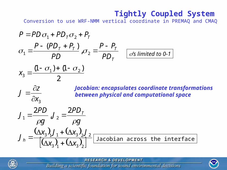
• Implemented the first step in tighter coupling between CMAQ and WRF-NMM computational grids CMAQ calculations using the WRF-NMM vertical coordinate Modifications to CMAQ to use the E-grid and rotated lat/lon

coordinate underway

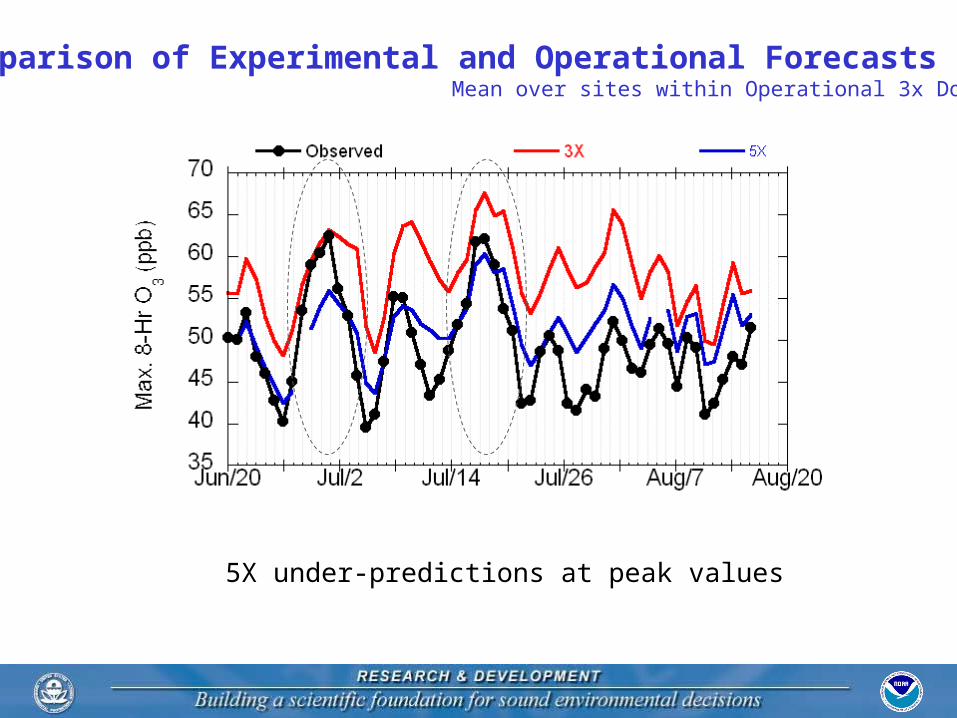
• Under-predictions for surface O3 in experimental predictions were found to arise from error in isoprene emission calculations Un-initialized lat/lon fields

Summary/Looking Ahead

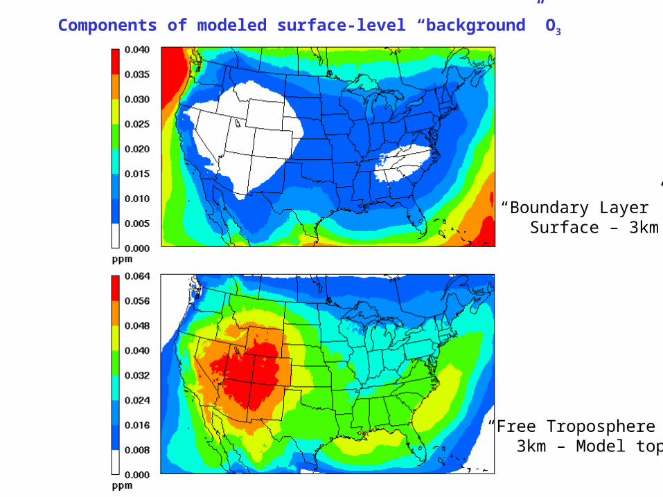
• Initial analysis of boundary tracers indicate that modeled O3 background values are strongly influenced by free tropospheric LBC values Locations at which O3 is over-predicted generally also

correspond to high background but low observed values

• Rigorous analysis of developmental PM simulations underway Seasonal trends/biases similar to hind-cast CMAQ

applications Speciated PM verifications with surface network (STN,

CASTNet, IMPROVE, SEARCH) and aloft (ICARTT) data

• Initial testing of a methodology for specifying “real-time” fire emissions tested Initial results are encouraging