THE COMPETITIVE SAVING MOTIVE:EVIDENCE FROM RISING SEX RATIOS AND SAVINGS RATES IN CHINA
Shang-Jin WeiXiaobo Zhang
Working Paper 15093http://www.nber.org/papers/w15093
NATIONAL BUREAU OF ECONOMIC RESEARCH1050 Massachusetts Avenue
Cambridge, MA 02138June 2009
The authors would like to thank Marcos Chamon, Avi Ebernstein, Lena Edlund, Roger Gordon, EdHopkins, Tatiana Kornienko, Justin Lin, Olivier Jeanne, Simon Johnson, Nancy Qian, JunshengZhang, and seminar participants at the NBER and various universities for helpful discussions, and JohnKlopfer, Lisa Moorman and Jin Yang for able research assistance. The views expressed herein arethose of the author(s) and do not necessarily reflect the views of the National Bureau of EconomicResearch.
The Competitive Saving Motive: Evidence from Rising Sex Ratios and Savings Rates in ChinaShang-Jin Wei and Xiaobo ZhangNBER Working Paper No. 15093June 2009JEL No. D1,F3
ABSTRACT
While the high savings rate in China has global impact, existing explanations are incomplete. Thispaper proposes a competitive saving motive as a new explanation: as the country experiences a risingsex ratio imbalance, the increased competition in the marriage market has induced the Chinese, especiallyparents with a son, to postpone consumption in favor of wealth accumulation. The pressure on savingsspills over to other households through higher costs of house purchases. Both cross-regional and household-levelevidence supports this hypothesis. This factor can potentially account for about half of the actual increasein the household savings rate during 1990-2007.
Shang-Jin WeiGraduate School of BusinessColumbia UniversityUris Hall 6193022 BroadwayNew York, NY 10027-6902and [email protected]
Xiaobo ZhangInternational Food Policy Research Institute2033 K Street, NWWashington, DC [email protected]
2
”… [A] surge in growth in China and a large number of other emerging market economies … led to an excess of global intended savings relative to intended capital investment. That ex ante excess of savings propelled global long-term interest rates progressively lower between early 2000 and 2005. That decline in long-term interest rates across a wide spectrum of countries statistically explains, and is the most likely major cause of, real-estate capitalization rates that declined and converged across the globe, resulting in the global housing price bubble.” Alan Greenspan, Wall Street Journal, March 11, 2009
1. Introduction
High savings rates in certain countries are said to be a major contributor to the
recent housing price bubbles and the global financial crisis by depressing global long-
term interest rate in the last decade (Greenspan, 2009). The Chinese national savings rate,
at about 50 percent of GDP in 2007, has caught special attention. This savings rate is high
in at least three senses. First, it is higher than most other countries, including East Asian
countries that are already known to have high savings rates. Second, it is higher than in
China’s own past: the gross domestic savings rate as a share of GDP rose by about 15
percentage points since 1990. Finally, it is higher than China’s already-high investment-
to-GDP ratio. China’s household savings are approximately half of its national savings.
(In 2007, the household savings as a share of the household disposal income was 30%).
The purpose of this paper is to test a new hypothesis regarding household savings
behavior using Chinese regional and household data. Before doing that, let us review
existing explanations in the literature. The first is the life cycle theory (Modigliani, 1970,
and Modigliani and Cao, 2004), which predicts that the savings rate rises with the share
of working age population in the total population. This explanation doesn’t appear to be
consistent with profile of savings at household level (Chamon and Prasad, 2008). The
second explanation has to do with a precautionary savings motive in combination with a
rise in income uncertainty, which is favored by Blanchard and Giavazzi (2005) and
Chamon and Prasad (2008). The problem is that while both pension systems and the
public provision of health care in China have been improved since 2003, household
savings as a share of disposable income rose sharply during the same period. This time
series pattern contradicts the precautionary motive theory. The third explanation is a low
level of financial development. This has the same difficulty as the last explanation since
the financial system is most likely more efficient today than a few years ago yet the
3
savings rate still rose. The fourth explanation is cultural norms. But cultural norms tend
to be persistent, and therefore are unlikely capable of explaining the visible rise in the
savings rate over the last two decades1.
In this paper, we suggest that an alternative competitive saving motive may be at
work: families with sons compete with each other to raise their savings rate in response to
ever rising pressure in the marriage market. Competitive saving by these families spills
over to greater savings by other families, possibly through raising the prices of non-
tradable goods such as housing. The increased pressure in the marriage market comes
from China’s rising sex ratio imbalance, which has made it progressively more difficult
for men to get married. As far as we know, we are the first in the literature to propose this
hypothesis as an explanation for a rising savings rate in China. Toward the end of the
paper, we argue that the explanation is likely applicable to many other countries as well.
We provide a series of evidence. First, across provinces, we show that the local
savings rate tends to be higher in regions and years in which the local sex ratio (for the
pre-marital age cohort) is higher. This continues to be true after we control for local
income, social safety net, the age profile of the local population, and province and year
fixed effects.
Second, in recognition of possible endogeneity of and measurement error in local
sex ratios, we employ instrumental variables where the local sex ratio for the pre-marital
age cohort is shown to be linked to local financial penalties for violating family planning
policies set more than a decade earlier (as Ebenstein, 2008, and Edlund et al, 2008, also
document). With two-stage least squares estimation, the effect of local sex ratios on local
savings rates remain positive and statistically significant. In fact, the point estimate
1 We do not study corporate savings behavior in this paper. The Chinese corporate savings rate has risen sharply in recent years, accounting now for about half of the national savings rate (Kuijs, 2006). The corporate savings behavior is a separate puzzle to be explained. The existing explanation suggests that a combination of state-ownership and windfalls in resource sectors is the primary driver. (The government savings rate is relatively moderate and has turned negative in 2008-09.) We note, however, that a recent paper by Bayoumi, Tong and Wei (2009) discusses China’s corporate savings rate in a global context and casts doubt on the usual interpretation. Because corporate savings rates have been rising globally (Bates, Kahle, and Stulz, 2005; and IMF, 2005), it turns out that the Chinese corporate savings rate is only modestly higher than those of other countries (by 2 percentage above the global average savings rate when comparing listed companies across countries). So differences in corporate savings are unlikely to be a big part of the cross country differences in national savings rates. Moreover, comparing corporate savings by Chinese firms of different ownership, in resource and non-resource sectors, Bayoumi, Tong and Wei (2009) do not find evidence that state-owned firms save more than private firms, or that the corporate savings rate is unusually high in resource sectors. This casts doubt on the notion that a high Chinese corporate savings rate is mainly a result of poor corporate governance and inefficiencies tied either to state-ownership or to windfalls in resource sectors.
4
becomes larger. This suggests that an increasing imbalance in the sex ratio causes a rise
in the savings rate.
Third, we examine household data using household surveys that cover 122 rural
counties and 70 cities. While households with a son typically save more than households
with a daughter, we do not regard this per se as supportive evidence of our hypothesis,
since other channels could account for this difference. Instead, the evidence that we find
compelling is that savings by otherwise identical households with a son tend to be greater
in regions with a higher local sex ratio. This is something clearly predicted by our
hypothesis, but not by any other existing explanations. In addition, we find that savings
by households with a daughter do not decline in regions with a high sex ratio, which is
consistent with our interpretation that the savings pressure on households with a son
spills over to other types of households. We discuss reasons that these patterns at the
household level are unlikely to be the outcome of some selection in the data.
Finally, we provide several supplementary pieces of evidence. We show that local
housing values indeed tend to be higher in regions with a higher local sex ratio, even after
taking into account local income. This is direct evidence that the competitive pressure on
households with a son in the marriage market may trigger other households to save more
just to cope with higher local housing costs. We also provide some evidence that
household level savings rates tend to be linked to a wedding event in a family in a
quantitatively significant way, and that a groom’s family tends to save more than a
bride’s family in preparation for the wedding.
We do not wish to claim that no combination of the existing explanations could
contribute to a higher savings rate. Instead, we suggest a competitive saving motive as an
additional explanation. The estimated effect of a rising sex ratio on the Chinese savings
rate is economically significant, and can be projected to become even more important in
the foreseeable future. Based on the point estimate (0.74) in the IV regression, a rise in
the sex ratio for the pre-marital age cohort from 1.05 to 1.14 (which is actual increase in
Chinese sex ratio for the age cohort of 7-21 from 1990-2007) would lead to a rise in the
savings rate by 6.7 percentage points, which is 48% of the actual increase in the
household savings rate. If we run separate regressions for rural and urban areas, we find
that the elasticity of the local savings rate with respect to the local sex ratio is larger in
5
rural areas than in urban areas. The increase in the rural sex ratio is estimated to account
about 53% of the actual increase in the rural savings rate from 1990 to 2007.
Because the sex ratio imbalance at birth has been increasing steadily since mid-
1980s, the imbalance for the pre-marital age cohort will almost surely be higher over the
next decade than in the last decade, even if the sex ratio at birth starts to be reserved soon.
This implies that the incremental savings rate that is stimulated by the competitive
savings motive will almost surely rise in importance in the near future.
A high savings rate in a large economy is a significant contributor to global
current account imbalances. Once one recognizes that the sex ratio imbalance is a
structural factor behind a rising savings rate, it should be clear that a discussion of global
imbalances that focuses narrowly on exchange rates or even social safety nets is
incomplete. Furthermore, policy actions that improve the economic status of women
could potentially reduce the sex ratio imbalance by reducing parental preference for sons
(Qian, 2008). A change in the family planning policy that relaxes birth quotas could also
reduce the imbalance. Because of their important implications for aggregate savings and
current account imbalances, these changes deserve more attention that they receive now.
The paper is organized in the following way. In Section 2, we develop the
argument more fully, lay out some caveats and possible answers to them, and make
connections to related literatures. In Section 3, we provide statistical evidence for our
hypothesis. Finally, in Section 4, we conclude and discuss possible future research. A
data appendix explains the sources and definitions of the main variables, including
measures of sex ratio imbalance and of savings rates.
2. Developing the argument: unbalanced sex ratios and competitive savings
In this section, we first document the evolution of the sex ratio imbalance in the
Chinese society over the last three decades. We then explain why this could trigger a race
to raise savings rate, and connect this discussion to related literature.
From unbalanced sex ratios to “bare branches”
Left to the nature, the sex ratio at birth (in a society without massive starvation) is
generally around 106 boys per 100 girls (with human biology compensating for a slightly
6
higher mortality rate for infant boys than girls). The sex ratio was balanced or slightly
below normal in the 1960s and 1970s (mostly likely due to malnutrition). The sex ratio at
birth in China was close to be normal in 1980 (with 106 boys per 100 girls), but climbed
steadily since the mid-1980s to over 120 boys for each 100 girls in 2005 (Li, 2007; Zhu,
Lu, and Hesketh, 2009) and estimated to be 124 boys/100 girls in 2007. By 2005, men
outnumbered women at age 25 or below by about 30 million. The excess men cannot be
married mathematically. The number of unmarried men -sometimes referred to as “bare
branches” in colloquial Chinese - continues to rise as the sex ratio imbalance deteriorates2.
Some men may partner off as gays, and others may emigrate or marry women
from other countries. Because the scale of the “bare branches” is so large – 30 million
men are more than the entire male population of Italy or of many other countries, and
because most “bare branches” come from low income households, actions by a small
portion of men do not provide a practical solution to the problem. In any case, a rising
sex ratio imbalance must imply a diminishing probability that a man will find a bride3.
From fear of becoming a “bare branch” to competitive savings
Most men have a desire to get married. It may be safer to say that, in an Asian
society, parents of a son strongly prefer for their son to be married. As the competition
for a dwindling pool of potential wives intensifies, the parents of a son (or a son himself)
will try harder to improve the son’s prospects for marriage. Postponing consumption and
raising the household savings rate is one such action that families may take. To be
successful, a family needs to save more than enough number of other competing families.
If all families think the same way, this leads to competitive saving. (Of course, in general
2 If some new-born girls are not reported by their parents with hopes to be pregnant again with a son, then the sex ratio imbalance at birth could be overstated in official statistics. To assess the quantitative importance of this possibility, we compare the sex ratio at birth in the 1990 population census with the sex ratio for the 10 years old in the 2000 census. It is reasonable to assume that parents would not hide their 10-year old girls from census-takers in 2000. First, those parents who would like to try for another child in 1990 most likely would have done so already within ten years, and have paid a fine for violating family planning policy by 2000. In addition, there were also positive incentives to report the girls who have reached school age since registration was required for (free) immunization shots and school attendance. Since the sex ratios for both the new-borns in 1990 and the 10 years old children in 2000 were 1.12, we conclude that the under-reported infant girls, as a proportion of total number of new-born girls, are not large enough to make a noticeable distortion to reported sex ratio imbalance. Zhu. Li and Hesketh (2009) reached the same conclusion with a somewhat different methodology. 3 A fraud has recently emerged in which some women pretend to be willing to marry bachelors in a rural area in return for a bride price (“cai li”) on the order of RMB 40,000 (about US$5900, or “five years’ worth of farm income”). The women would then run away after the wedding with the bride price (“It’s cold cash, not cold feet, motivating runaway brides in China,” by Mei Fong, Wall Street Journal, June 5, 2009)
7
equilibrium, the total number of unmarried men will not be changed by household
savings decision. But an individual family’s desire to improve marriage prospects for its
son may lead all families with a son to compete to increase their savings.]
The idea that accumulating more wealth may improve one’s chance in the
marriage market is not unique to China. For example, pop star Madonna has declared in
the hit song, “Material Girl,” that: “We are living in a material world/ and I am a material
girl/Some boys try and some boys lie but/ I don’t let them play/ Only boys who save their
pennies/ make my rainy day.” So she sees a connection between a man’s savings rate and
his success in dating. To be clear, our hypothesis does not require women to be material
girls (in China or elsewhere). Indeed, other factors can be important for success in finding
a spouse. But other things being equal, as long as more wealth improves a man’s
likelihood for marriage, parents with a son (or a son himself) will be encouraged to raise
their savings rates. Many factors (such as health and appearance) are difficult to control,
but the savings rate is one such thing that parents or men themselves can act on. However,
we are not saying that the savings behavior is the only variable that is altered by a rising
sex ratio. Instead, parents with a son may do all things in their power to improve their
son’s marriage prospect, including perhaps investing more in their son’s education, and
pushing him to work harder. The hypothesis in the current paper is that postponing
parents’ consumption and raising their savings rate may be one such variable that
responds positively to a rising sex ratio.
For the sex ratio to affect household savings rates, parents don’t have to know
local sex ratio statistics. There is an invisible hand at work. Consider two otherwise
identical households with a son, one in a region with a high sex ratio, and the other in a
region with a low sex ratio. Parents in the first region would observe or be told by
relatives or colleagues with a son that it is very expensive for their sons to find a
girlfriend and to marry. The expectation for how much the parents (or the sons) need to
contribute to their son’s new household, given costs of housing, cars, furniture, or
honeymoons, would differ in the two regions. The types of furniture, cars and
honeymoons, and local housing prices may already reflect the degree of competition in a
local marriage market, and thus affect the savings required of parents with a son. In other
8
words, even without knowledge of local sex ratio statistics, parents with a son may make
savings decisions that reflect the local sex ratio.
The initial inspiration for the hypothesis comes (from our visits to the National
Zoo in Washington DC, and) from the literature on evolutionary biology. In nature, male
sea lions or walruses tend to be physically larger than corresponding females; in fact, this
pattern holds for most species. A leading hypothesis for why this occurs, sexual
dimorphism, conjectures that because bigger and stronger males have an advantage in
competing for and retaining females, differences in size are reinforced over time by
natural selection (Weckerly 1998). It is likely that humans had to do the same a long time
ago; that is why men, on average, are somewhat taller and larger than women. By now,
the (sexual) returns to progressively larger males are much lower, if not negative. Men
may discover that possessing a larger house, a bigger savings account, and more general
wealth is a more effective mating strategy.
Existing literature, potential caveats, and counter-arguments
No other paper in the existing empirical literature that we are aware of makes a
connection between sex ratios and savings rates. Nonetheless, a relevant economics
literature is the work on status goods, positional goods, and social norms (e.g., Cole,
Mailath and Postlewaite, 1992; Hopkins and Kornienko, 2004 and 2009). When allowing
certain goods to offer utility beyond their direct consumption value (i.e., through “status,”
which in turn could affect the prospect of finding a marriage partner), it is easy to show
that consumption and savings behavior can be altered. It is important to point out,
however, that the effect of a rising sex ratio imbalance on savings rates is conceptually
ambiguous. In particular, when competition in the marriage market increases, men (or
their parents) may compete by increasing their conspicuous consumption, if conspicuous
consumption effectively signals their attractiveness; this would result in a decline in the
savings rate. Our response is that, while conspicuous consumption may increase the
frequency of dating, the probability of securing a marriage partner may depend more on
showing substantial wealth than on showing off a few flashy goods. Furthermore, a
visible way to demonstrate a man’s desirability is by owning a larger house (at least in a
developing country like China), which requires a larger savings before the purchase is
9
made than otherwise. Both signaling strategies can induce households with a son to raise
their savings rate. In any case, it is an empirical question as to whether savings rates are
positively or negatively related to sex ratio imbalances.
The theoretical models in Hopkins (2009) and Hopkins and Kornienko (2009)
could be interpreted to predict that a rise in sex ratio imbalances leads to a rise in savings
rates. In a possible reading of their models, men compete for potential wives through
effort (including by raising their savings rate). Assume that the reward for a higher
savings rate is a better chance to win a wife. Men with the lowest savings rates, on the
other hand, may not find a wife. As the fraction of men who may stay unmarried
increases, men (without coordination) compete by saving more. The resulting level of
savings for men is inefficiently high: if all men were to cut their savings by the same
amount, the chance for each of them to be matched with a wife would stay the same, but
they would have avoided postponing consumption unnecessarily.
When the savings effect dominates the conspicuous consumption effect for
parents with a son (or unmarried men), would parents with a girl (or unmarried women)
save less since a rising sex ratio is a favorable development for them? Indeed, could the
reduction in their savings be so much as to completely offset the increase in savings by
parents with a son or unmarried men? In a way, we can wait for the data to tell us the
answer. Here, it is useful to point out the existence of an opposing force that could
potentially raise the savings rate even by parents with a daughter. That force is the price
of housing. Parents with a son (or unmarried men) may attempt to increase their
competitiveness by buying a larger house, and may bid up housing prices in a region with
an unbalanced sex ratio. As a consequence, even parents with a daughter have to save
more in order to afford housing. This is a spillover effect4.
This discussion has clear implications for the empirical work. First, we need to
estimate the net effect of higher local sex ratios on local savings rates. Second, it would
be useful to check how savings by households with a son or with a daughter respond to
local sex ratios. Third, it would be informative to check if local housing prices are indeed
linked to local sex ratios (holding constant other factors).
4h When all men save more, the reward for savings by women or parents with a daughter increases, if wealthier men also prefer relatively wealthy women. As a result, parents with a daughter are also more willing to save. For a theoretical model that may deliver this result, see Peters and Siow, 2002. This could be an additional spillover channel.
10
Determinants of sex ratio imbalance
Sex ratio imbalance comes almost entirely from sex selective abortions. This, in
turn, results from a combination of three factors: (a) parental preference for sons; (b)
some limit to the number of children a couple is allowed or wants to have, which for the
Chinese is a strict family planning policy; and (c) availability of inexpensive technology
to screen the sex of a fetus (Ultrasound B in particular) and to perform abortions.
Our empirical work will start with regressions that assume exogenous sex ratios.
This assumption can be justified by recognizing that parental preference for sons is part
of a culture, and as such, it changes only very slowly. Korea has experienced a sustained
increase in its sex ratio imbalance for about 25 to 30 years, which has only recently
started to decline; this evidence is consistent with our assumption (Guilmoto, 2007).
We nonetheless also report instrumental variable regressions that allow for
potential endogeneity of (and measurement error in) sex ratios. The instrumental
variables for sex ratio in the pre-marital age cohort explore regional variations in the
financial penalty for violating birth quotas, set by regional governments years before
newborns grow to marriageable age.
3. Statistical Evidence
Since 1980, both the sex ratio for marriage-age youths and the savings rate in
China have been rising. In Figure 1, we present a time series plot of standardized versions
of both variables,5 with the sex ratio at birth lagged by twenty years. The sex ratio is
lagged since the median age of first marriage for Chinese women is about 20. The two
standardized variables, visually, are highly correlated (the actual correlation coefficient is
0.822). While this is highly suggestive, it is not a rigorous proof by itself.
Panel regressions across Chinese provinces during 1980-2007
We start by examining provincial-level data for any association between local
savings rates and local sex ratios. We perform a panel fixed effects regression that links a
location j’s savings rate in year t with the sex ratio for the appropriate age cohort in that
same location and year, controlling for location fixed effects, year fixed effects, and other
factors. To be precise, our specification is the following:
Savings_ratej,t = β Sex_ratio j,t +X j, t Γj,t + province fixed effects + year dummies +e j,t
Following Chamon and Prasad (2008), we define the local savings rate by log (income
net of taxes / living expenditure).6 This definition is less susceptible to extreme values,
and makes the error term more likely to satisfy the normality assumption. We cluster the
standard errors by province.
Ideally, we would like to know sex ratios for a fixed age cohort in every region
and in every year. However, such data are not available as the Chinese population census
is carried out only once every few years (in 1982, 1990 and 2000). Moreover, only the
2000 census offers public data for individual age groups at the provincial level. Given
these constraints, we make the following short cut: we focus on the sex ratios for the age
cohort 7-21 in all years, inferred from the 2000 population census. For the age cohort 7-
21 in 2007, we infer their sex ratio from the age cohort 0-19 in the 2000 census, since the
two groups should theoretically be the same. Similarly, for the age cohort 7-21 in 1990,
we infer their statistics from the cohort 17-31 in the 2000 census; and so on.
A caveat with this method is that the actual sex ratio is likely to be different from
the inferred one for all years other than 2000. In particular, because the mortality rates for
boys and young men are generally slightly higher than those for girls and young women,
we may under-estimate the true sex ratios for years before 2000 and over-estimate them
for years after 2000. However, under the assumption that measurement errors are
common across all regions in any given year (but may vary from year to year), we can
eliminate the effect of measurement errors by including year fixed effects in regressions.
As control variables, we include both log income and proportions of the local
population in the age brackets of 0-19 and 20-59, respectively. Table 1a presents the
summary statistics of the major variables used in the provincial level analysis. Table 1b
6 Income and expenditure data, which are aggregated based on nationwide rural and urban household surveys, are from various issues of China Statistical Yearbooks.
12
lists the outlier provinces – those with the highest and lowest sex ratios in various years.
For example, in 2005, Jiangxi and Shaanxi had the highest sex ratios at birth, both in
excess of 130 boys per 100 girls. At the other end of the spectrum, Tibet, Liaoning, Jilin,
and Xinjiang had the lowest sex ratios at birth, with 109 boys or less per 100 girls.
In Column 1 of Table 2, we report regression results with only sex ratio, income
and population shares for two age groups as the regressors (plus province and year fixed
effects). The effect of local income on local savings rates is positive: a one percent
increase in local income is associated with local savings rate 0.26 percentage points
higher. The coefficient of local sex ratio (for the age cohort 7-21) is 0.39 and statistically
different from zero at the 5% level. In other words, the local savings rates tend to be
higher in regions with a more imbalanced sex ratio.
The age profile of local populations produces some puzzling patterns. In contrast
to the prediction of the life cycle hypothesis, the share of working age population (the age
cohort of 20-59) has a negative coefficient. This means that old-age households and
households with children save more than do households in between. We note that this is
consistent with the notion that parents save more when they have children, and that old
people save more either because they have a strong bequest motive, or because they
realize their financial need in the old age is greater. Regardless of these explanations, we
note that similar patterns are documented in Chamon and Prasad (2008).
The existing literature has hypothesized that rising income and job uncertainty is
what motivates the Chinese to save more. In Column 2, we use the proportion of local
labor force that work for state-owned firms or government agencies as a proxy of the
degree of job security. Under the precautionary savings hypothesis, the savings rate
should decline with better job security. The coefficient indeed has a negative coefficient
(-0.14); however, it is not statistically significant. In any case, the coefficient on sex ratio
is still positive and significant. The point estimate (0.70) is now substantially larger.
Because men and women may both have different savings rates and different
income levels, one might worry that income inequality could affect local savings rates
directly, and that a sex ratio imbalance is simply a proxy for earnings inequality. For a
subset of provinces and years, we can measure local income inequality directly by the
13
Gini coefficient.7 In Column 3 of Table 2, we add the local Gini coefficient as an
additional control. While the coefficient is positive – consistent with the idea that a
greater inequality is associated with a higher savings rate, it is not statistically different
from zero. With this much reduced sample, the coefficient on the local sex ratio is still
positive and statistically significant. The point estimate jumps to 0.92.
In Column 4 of Table 2, we include local life expectancy as an additional
regressor to account for the possibility that households save more when they expect to
live longer.8 We also the share of local labor force enrolled in social security as a proxy
for the extent of local social safety net. Neither coefficient is statistically different from
zero. This suggests that inadequacy of social safety net does not appear to be as
quantitatively important in explaining savings rates as commonly believed. We make this
observation with one important caveat: this does not rule out the possibility that every
region’s saving rate has been made higher due to a poor national social safety net.
Caroll, Overland, and Weil (2008) point out that, assuming habit formation in
consumption, savings rate should tend to be higher in a fast-growing economy since
consumption growth may not catch up with income growth immediately. In the last
column of Table 2, we add the local growth rate of the preceding five years. This variable
turns out to be insignificant, and the point estimate is in fact negative, which would have
been consistent with a more standard model of consumption smoothing without habit
formation. In any case, the coefficient on local sex ratio is still positive (0.34) and
statistically significant. Across the columns in Table 2, the positive association between a
high local sex ratio and a high local savings rate is robust and statistically significant.
Rural versus urban areas
Urban and rural areas differ in income, education level, and coverage of social
safety nets. Parental preference for a son is also known to be stronger in rural areas.
Perhaps most importantly, local marriage markets may work differently in rural and
urban areas. A majority of marriages in rural areas take place between a man and a
7 The Gini coefficients are obtained from Ravallion and Chen (2007). The data are available for 29 provinces in 1988, 1990 and 1993, and 28 provinces in 1996 and 1999 for the urban sample, and 27 provinces in 1988, and 28 provinces in all other years for the rural sample. The overall Gini coefficients at the province level are approximated by weighted average of rural and urban Gini coefficients. 8 Life expectancy at the provincial level is only available in the three census years (1982, 1990 and 2000).
14
woman from the same county9. Most migrant workers either get married before leaving
their homes to work in a city, or return to their villages to get married. In comparison, it
is somewhat more common for marriages in cities involving a husband or a wife from
outside the city. An implication of this difference in the marriage market is that the same
local sex ratio imbalance may exert a smaller competitive pressure on men in a city than
in a rural area. For these reasons, one may expect local savings rates to be more sensitive
to local sex ratio imbalances in rural areas than in urban areas. Therefore, additional
confirmation of the hypothesis may be obtained by running separate regressions for these
two areas. The control variables are the same as those in Table 2 to the extent they are
available for separate rural and urban areas.
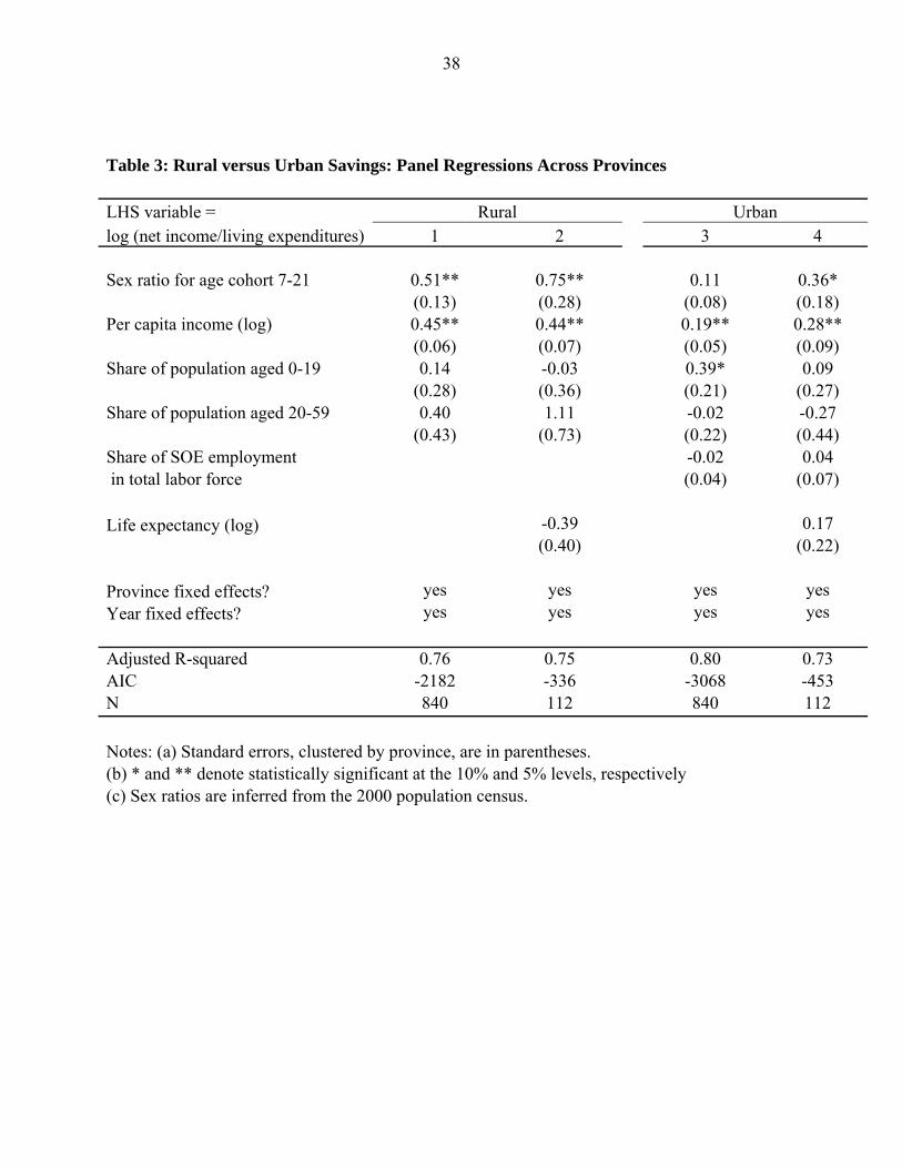
The results are reported in Table 3. It is interesting to note that the estimated
elasticity of local savings rates with respect to sex ratios is indeed greater for rural areas
than for urban areas (0.75 versus 0.36, respectively, from Columns 2 and 4 of Table 3).
Instrumental variable regressions
The degree of a local sex ratio imbalance for the pre-marital age cohort (7-21) is
pre-determined with respect to local savings decisions by construction, since the sex ratio
is determined by parental decisions -- whether to undertake a sex selective abortion
before a child is born -- taken many years prior to the corresponding savings variables in
the regressions. This helps to justify the panel regressions reported in Tables 2 and 3.
Nonetheless, one has to think hard about the possibility that sex ratio is endogenous, or
that sex ratio is a proxy for something else that affects savings decision directly. For
example, factors that affect sex-specific earnings in a region could simultaneously
determine both a preference for sons and household savings decisions. In addition, as we
noted earlier, local sex ratios may be measured with errors since they are inferred from
the 2000 population census. In either case, the estimated elasticity of the local savings
with respect to the local sex ratio may be biased.
A solution to both the endogeneity issue and measurement errors is to employ an
instrumental variable approach, which we turn to now. A key determinant of the sex ratio
9 According to the China Population Census 2000, about 10% of people migrate to places outside their registered counties or districts in 2000. Among them, only 2.5% list marriage or family reunion as a major reason of migration.
15
imbalance is a strict family planning policy introduced in the early 1980s.10 We explore
two determinants of local sex ratios that are unlikely to be affected by local savings rates,
and for which we can get data. First, while the goals of family planning are national, the
enforcement is local. Eberstein (2008) proposes to use regional variations in the monetary
penalties for violating the family planning policy as an instrument for the local sex ratio.
Using data collected by Scharping (2003) and extending them to more recent years,
Eberstein focuses on two dimensions of penalties: (a) a monetary penalty for the violation
of policy, expressed as a percent of annual income in the province, and (b) a dummy for
the existence of extra penalty for having higher order unsanctioned births (e.g., for having
a 3rd child in a 1-child zone, or for having a 4th child in a 2-child zone). These two
variables are part of our set of instruments too. Second, while the Han ethnic groups faces
a strict birth quota, the rest of the population (i.e., the 50 some ethnic minority groups) do
not face or face much less stringent quotas. (The government allowed the exemption,
possibly to avoid criticisms for using the family planning policy to marginalize minority
groups). Since non-Han Chinese are not uniformly distributed across space, this variation
offers one more possible instrument (Bulte, Heerink and Zhang, 2009).11
In Table 4, we report the first-stage regressions for the IV regressions that link
local sex ratios to their determinants, with both financial penalties and minority shares
lagged by 14 years (to match the median birth year for the age cohort 7-21). Both types of
variables appear to be related to sex ratios. First, more severe financial penalties -- set in
a decade earlier -- are indeed associated with a more unbalanced sex ratio. Second, the
proportion of people not subject to birth quotas is negatively related to local sex ratio
imbalance. The adjusted R-squared for the first-stage regressions is in excess of 60%.
In Column 1 of Table 5, we report the 2SLS estimation results for local savings
rates where the local sex ratio is instrumented by the three variables described above.
10 China’s family planning policy, commonly known as the “one-child policy,” has many nuances. Since 1979, the central government has stipulated that Han families in the urban areas should normally have only child (with some exceptions). Han Chinese are in the majority ethnic group, accounting for about 95% of the Chinese population at the time the policy was introduced. Families in rural areas can generally have a second child if the first one is a daughter (this is referred to as the “1.5 children policy” by Eberstein, 2008). Ethnic minority (i.e., non-Han) groups are generally exempted from birth quotas. Non-Han groups account for a relatively significant share of local populations in Xinjiang, Yunnan, Ganshu, Guizhou, Inner Mongolia, and Tibet. 11 In principle, variations in the cost of sex screening technology especially the use of an Ultrasound B machine, and the economic status of women (such as that documented in Qian 2008) could also be candidates for instrumental variables. Unfortunately, we do not have the relevant data. Note, however, for the validity of the instrumental variable regressions, we do not need a complete list of the determinants of local sex ratio in the first stage.
16
While a Durbin-Wu-Hausman test rejects the null that the sex ratio is exogenous (with a
p-value of 0.03), a Hansen’s J statistic for over-identification fails to reject the null that
the instrumental variables are valid (with a p-value of 0.30). With the 2SLS procedure,
the local sex ratio continues to have a positive coefficient that is statistically different
from zero. The point estimates, 0.74, is in fact larger than most corresponding estimates
in Table 2. This suggests that an attenuation bias from measurement errors might have
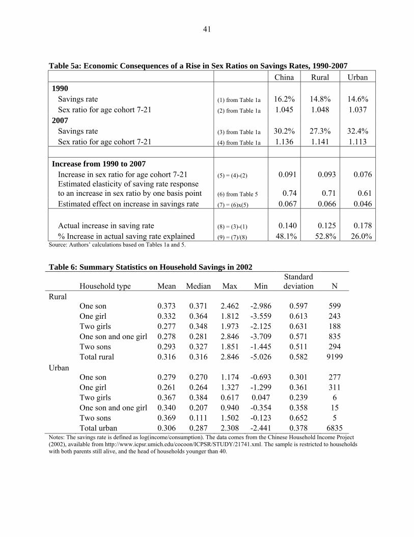
outweighed an endogeneity bias in the original panel regressions. Based on the point
estimate in Column 1 (0.74), an increase in the sex ratio for the age cohort 7-21 from
1.045 in 1990 to 1.136 in 2007, leads to a rise in the savings rate by 6.7 percentage points,
accounting for 48% of the actual increase in Chinese savings rate during this period
(details of the calculation can be found in Table 5a).
We also find that richer regions save more. A one percent higher per capita
income is associated with a higher savings rate by 0.27 percent. Regions with more
people working in the state sector save less. An increase in the share of state sector
employment in local population by one percentage point is associated with a reduction in
local savings rate by 0.24 percentage points. The last finding supports a precautionary
savings motive: If more public sector employment implies less income and job
uncertainty, then there is less need to save. We do not find evidence that the age profile
of the local population matters per se, which suggests that the life cycle hypothesis is not
supported in the data (as in Chamon and Prasad, 2008).
In Column 2 of Table 5, we replicate the 2SLS estimation but excluding the share
of minorities in local population from the set of instruments. Even though the Hansen’s J
test in the first column suggests that all three instrumental variables, including the
minority share, are valid in a purely statistical sense, we act conservatively here and
allow for the possibility that non-Han Chinese have a different desired rate of savings and
thus should not be in the set of instruments. In this case, the local sex ratio continues to
exhibit a positive and statistically significant coefficient, with the point estimate
becoming even larger (0.89). An increase in the sex ratio for the age cohort 7-21 from
1.05 in 1990 to 1.14 in 2007, would now lead to a rise in the savings rate by 8.0
percentage points (=0.09 x 0.89 x 100), accounting for 50% of the actual increase in
Chinese savings rate ( =6.66/[(0.31-0.15)x100] ). With household level regressions to be
17
reported later (Tables 7-9), we find no robust evidence that savings by households headed
by ethnic minorities behave differently from their Han counterparts in a given location. In
other words, minority shares are unlikely to affect savings rates directly without going
through local sex ratios. Therefore, we prefer those 2SLS estimates in Column 1 in which
all three instruments are used.
In Columns 3 and 4 of Table 5, we apply the three instruments for sex ratio to
2SLS estimation where the dependent variable is either the rural or the urban savings rate.
We confirm the results in the earlier panel regression: a higher local sex ratio raises local
savings rates in both areas. The reaction of the local savings rate to a change in the sex
ratio is stronger in rural areas. An increase in the rural sex ratio from 1.048 to 1.141 (the
actual mean increase from 1990 to 2007) would lead to an increase in the rural savings
rate by about 6.6 percentage points, or about 53% of the actual increase in the savings
rate during this period12. For the urban areas, an increase in the sex ratio from 1.037 in
1990 to 1.113 in 2007 would raise the savings rate by 4.6 percentage points, accounting
for about 26% of the actual rise in the savings rate. (Table 5a presents the calculations).
Household-level evidence
It is useful to go beyond regional aggregate comparisons and look at evidence at
the household level. From data in the Chinese Household Income Project (CHIP) of 2002,
which covers 122 rural counties and 70 cities, we construct a sub-sample of households
with one or two children and a household head younger than 40.13 Since most unmarried
young people live with their parents, the survey does not contain many observations of an
unmarried young man or woman as the household head. Therefore, we are not able to
analyze such households directly.
One may be tempted to compare savings rates for households with sons and those
with daughters. But this comparison is not particularly informative for our hypothesis.
Under the hypothesis of a competitive saving motive, one expects that families with a son
12 In the rural savings equation, it is useful to note that the Durbin-Wu-Hausman test does not reject the null that the sex ratio regressor is uncorrelated with the error term in the original OLS (panel) regressions in Table 3. In this case, one may prefer the estimates in Columns 1-2 of Table 3 on the efficiency ground. (At it turns out, the Hansen’s J test in Table 5 suggests that the IV’s do not work well for the rural savings regression.) 13 We place an age limit of 40 for heads of households with an aim to exclude households with some older children (who have left home) and some younger ones. They may not be comparable to households with only younger children.
18
to save more, if other things are held constant. However, other things cannot be held
constant because parents may not expect to get the same degree of help from their
daughters than from their sons as they age, especially in a rural area where a woman
moves to live with a man’s family after the marriage. In other words, families with only
daughters may need to save more to prepare for old age. For this reason, a direct
comparison of the savings rates between these two types of households is not informative
for our purpose.
In any case, Table 6 reports average saving rates for households with children of
different genders. In both rural and urban areas, households with a son have a moderately
higher savings rate than those with a daughter (37% versus 33% in rural areas, and 30%
versus 26% in urban areas). However, none of the differences in savings rates is
statistically significant; the standard deviation of the savings rate within any type of
household easily overwhelms the difference in the savings rate between any two types of
household. Of course, large standard deviations also suggest the presence of considerable
noise in the savings data. In any case, we cannot confirm or reject our hypothesis by
comparing the savings rates across household types in this way.
Our hypothesis, however, implies a particular regional variation in saving rates:
households with a son should save more in a region with a more unbalanced sex ratio,
holding constant family income and other characteristics. Moreover, this pattern is not
predicted by either the life-cycle theory or by existing precautionary savings motive
hypotheses. Therefore, examining the relationship between household savings rates and
local sex ratios may be particularly informative for testing our hypothesis.
We can also examine the relationship between the savings rate by households
with a daughter and the local sex ratio. This helps us to check the presence of a spillover
channel in savings pressure from households with a son to other households. If the
spillover channel operates through housing prices, it is likely to be stronger in the urban
areas as houses are more likely to be purchased from the local market (as opposed to
being built on the occupants’ own land in rural areas).
The regression results for the rural sample are presented in Table 7. The first four
regressions are performed on a full sample. The last four regressions are on a sample
where the top and bottom 5% of savings rate outliers are removed. Since the large
19
standard deviations in the savings rates reported in Table 6 likely reflect noise, we place
more trust in the results from regressions where the outliers are removed. We therefore
focus our discussion on the results reported in the last four columns of Table 7. (The
results from the first four columns largely confirm the same patterns.) The regressions
control for family income, children’s ages, characteristics of the head of household (sex,
education, and ethnic background), and local income inequality. It also controls for health
shocks to the family by a dummy denoting “poor health” if the family has a disabled or
severely ill member.
Column 5 of Table 7 relates savings by households with a son to local sex ratios
and other determinants of savings rate. We find that the local sex ratio has a strongly
positive effect on the household savings rate. An increase in the local sex ratio from 1.05
to 1.14 (the mean increase in rural China from 1990 to 2007) is associated with a higher
household savings rate by 12.2 percentage points, which is economically large. In
comparison, Column 6 of Table 7 reports the regression concerning savings by
households with a daughter. The coefficient on the local sex ratio is negative (-0.05),
consistent with the possibility that households with a daughter take advantage of a higher
sex ratio imbalance in their favor by saving less. (Surveys of rural households in Guizhou
province of China conducted by one of the authors in 2005 and 2007 show that a bride’s
family often expects a financial transfer from a groom’s family). However, the coefficient
is statistically insignificant. This may reflect an offsetting effect from a spillover in the
savings pressure that we have discussed.
In Columns 7 Table 7, we report a regression on savings by households with two
daughters. The coefficient on local sex ratio is more negative in this case (-0.36) than in
the one-daughter case (-0.05). This is consistent with the notion that a higher sex ratio
imbalance per se raises the bargaining power of the families for every daughter they have.
However, the coefficient is still statistically insignificant, possibly reflecting a strong
offsetting effect from the spillover of competitive savings by families with a son.
In Columns 8 Table 7, we report a regression on savings by households with a son
and a daughter. (It is relatively uncommon in the sample to have two sons due to the
family planning policy). The coefficient on the local sex ratio is positive (0.16),
20
somewhere in between the son-only case and the daughter(s)-only case. However, it is
also statistically insignificant.
Overall, the rural savings behavior is consistent with the competitive savings
motive. Households with a son save more in regions with a more unbalanced sex ratio.
Other households do not (significantly) reduce their savings in response. The elasticity of
the savings by households with a son with respect to the local sex ratio (1.36) is
substantially greater than the elasticity of the regional savings to the regional sex ratio
reported in early panel regressions. This is sensible since the latter reflects a weighted
average of the elasticities across different types of households.
In Table 8, we examine urban savings. We study only households with a son or a
daughter because it is relatively rare to have households with two children in the urban
sample due to the family planning policy. Again, we focus on the last four columns that
exclude the top and bottom 5% outliers in terms of savings rate. In Column 3 of Table 8,
we regress savings by households with a son on the local sex ratio and other controls. The
coefficient on the local sex ratio is positive (1.40) and statistically significant. An
increase in the sex ratio from 1.05 to 1.11 would be associated with a higher savings rate
by 8.4 percentage points, an economically large magnitude.
In Column 4 of Table 8, we examine savings by households with a daughter.
Interestingly, we find that these households’ savings rates are not sensitive to the local
sex ratio. This is similar to the rural sample. We interpret the insignificant coefficient as
reflecting a cancellation of two opposing forces: a spillover from competitive savings
pressure, and an opportunity for households with a daughter to take advantage of a
change in the local sex ratio imbalance in their favor.
In the last two columns of Table 8, we pool the two types of households in one
regression. In Column 5, we add a dummy for households with a son and an interaction
term between the local sex ratio and the dummy for households with a son. We find the
coefficient on the son dummy to be negative and significant. In contrast, the interaction
term is positive and significant. In other words, a combination of having a son and a
higher local sex ratio is associated with a higher household savings rate. Since the three
regressors (the sex ratio, the son dummy, and their interactions) are likely to be highly
correlated, in the last column, we drop the interaction term. In that case, the son dummy
21
is no longer different from zero statistically, but the local sex ratio is positive (0.90) and
significant. We conclude from the last two columns that having a son per se does not
raise a household’s savings rate; instead, a combination of having a son and facing a
scarcity of local women makes these families react by raising their savings rates.
For the urban sample, we have more information about the employer
characteristics of the family members. We can therefore construct a set of additional
proxies to detect a precautionary savings motive. We create an indicator variable for
households with no access to public health insurance, one for those with at least one
family member who has been laid off, one for those with at least one family member
employed in a state-owned company, one for those with at least one family member
working in a company that has recently experienced a reorganization (and hence at risk of
being laid off), and another one for households with a member working for an employer
that has been losing money. In addition, we create a dummy for households that currently
rent, rather than own, an apartment. All of these variables provide a richer set of
descriptions of the vulnerability of a family to income uncertainty.
The regressions with this expanded set of controls are reported in Table 9. We
again focus on the last four columns that exclude outliers in the data. Among the new
regressors, the coefficient on the dummy for households that are renters is negative and
statistically significant (-0.06). We conjecture that these households face a greater degree
of liquidity constraint, and may not be able to save as much as they desire. The
coefficient on households without public insurance is positive and significant Columns 4-
6 of Table 9. Such a pattern is consistent with a precautionary savings motive. However,
somewhat puzzlingly, the coefficient for a dummy for family members working in a
state-owned enterprise is also positive and significant in the same regressions. If SOE
employment implies less job uncertainty, then this contradicts the precautionary savings
motive. On the other hand, if current SOEs are expected to be downsized, restructured, or
privatized in the future, employment in an SOE could still mean income uncertainty.
After all, many previous SOEs have been downsized or privatized.
Our primary interest remains with the coefficients on the local sex ratio. For
families with a son (see Column 3 of Table 9), the elasticity of the local savings rate with
respect to the local sex ratio is positive (1.17) and statistically significant. For families
22
with a daughter (see Column 4 of Table 9), the elasticity is positive but not statistically
significant. These patterns are in line with our earlier findings, and consistent with a
competitive saving motive. In the last two columns of Table 9, we again find that having
a son per se would not lead to a higher household savings rate. It takes a higher local sex
ratio imbalance for households with a son to raise their savings rates.
Discussion of alternative interpretations
Could the local sex ratio be correlated with some omitted or unobserved variable
that also affect household savings decision? In Tables 7-9, we control for a long list of
variables that may reflect life-cycle considerations (e.g., age of head of household and
age of children) and precautionary savings motives (e.g., dummies for poor health of
family members, job loss by family members, employment in the public sector,
enrollment in public insurance, or employment in firms that experience losses or re-
organization). Nonetheless, there may be certain dimensions of quality of local social
safety net, growth potential, or income uncertainty that may affect household savings
decisions but have not been included in our long list of controls. One may imagine a
region with more intrinsic income uncertainty, or a greater local aversion to a given
uncertainty, may simultaneously exhibit a higher local sex ratio imbalance and a higher
local savings rate. There may be a positive association between household savings and
local sex ratios, but it does not reflect a causal relationship from the sex ratio to the
savings rate. Can we rule this out?
If the local sex ratio is suspected of reflecting an unobserved location-specific
shock, we can rule this out relatively easily. A pure location-specific shock should affect
savings by all households in the same region in the same way. But that is not what we
find. Instead, only the savings by those households with a son react strongly and
positively to a rise in the local sex ratio, while savings by households with a daughter do
not (after excluding outliers).
The next possibility is far more challenging: could a sex ratio imbalance reflect
something that is both location and household specific? For example, a region may have
an unusually high level of income uncertainty that is common to all households, but some
households care about this uncertainty more than others. Those households with a
23
stronger aversion to uncertainty may engage in a sex selective abortion more aggressively
and save more at the same time. This may generate a pattern reported in Tables 7-9. By
construction, selection at both household and location level is much harder to rule out
since our unit of observation is at the same level.
However, there are good reasons to think that if we focus on households with a
single child, such selection is unlikely to be quantitatively significant. Ebenstein (2008)
shows that sex ratio imbalance is overwhelmingly a result of sex selective abortions at
higher orders of birth. That is, the sex ratio for first-born children is close to normal. This
is particularly true in rural areas: since a second child is officially permitted if the first
child is a girl, and since many families exhibit a preference for a balanced sex ratio (one
boy and one girl) over having two boys (Ebenstein, 2008), there is very little reason to
perform sex selective abortions on the first pregnancies. However, the sex ratio at birth
goes up substantially over time for the second-born children and becomes even more
skewed for higher order births. Similarly, Zhu, Lu and Hesketh in an article on sex ratio
imbalance in China published in the British Medical Journal (2009) concludes that: “The
sex ratio at birth was close to normal for first order births but rose steeply for second
order births, especially in rural areas, where it reached 146 (in 2005).” This suggests that
the first son (or daughter) is unlikely to result from a sex selective abortion. Going back
to Tables 7, if we restrict attention to households with only one child, we clearly see that
those with a son exhibit a strongly positive elasticity of savings with respect to local sex
ratio, but those with a daughter do not. Comparing the results across Tables 7-9, we see
that the sensitivity of savings by a household with a son to the local sex ratio is stronger
in rural areas.
Savings rates and wedding events
Our hypothesis connects sex ratio to savings rate through pressure in the marriage
market. It is therefore desirable to have some evidence on whether household savings
rates actually vary with the timing of a wedding event in the family, and whether the
pattern differs between households with a son and those with a daughter. Unfortunately,
most household surveys do not ask about the timing or costs of wedding events in a way
24
that would allow one to trace out a time series profile of a household’s savings rate with
respect to wedding events.
Fortunately, for 26 natural villages (in three administrative villages) in Guizhou
Province, two rounds of household census were conducted in 2005 and 2007 by the
International Food Policy Research Institute (IFPRI) (with one of the authors as a project
leader). In each round, all households were asked their income and expenditure in the
previous year. The second round survey also includes recall data of major events, such as
weddings in a family, in the preceding ten years. From this data set, we construct a time
series profile of a “typical” household’s savings rate with respect to the timing of
wedding, i.e., the savings rate 2 years before the wedding, 1 year before the wedding, the
year of the wedding, and so on, all the way to 4 years after the wedding. By a “typical”
household, we mean that we take average across households with the same number of
years distant from a wedding. For example, for the savings rate in the year of wedding,
we average the savings rate across all households that have a wedding in that year.
Because the number of households that have a wedding event is relatively small, we do
not have enough statistical power to include control variables or to perform formal tests
on the differences in the average savings rates across years or across household types. So
the result should be interpreted with these limitations in mind.
Figure 3 plots the time profile of a representative household savings rate for
groom and bride families, separately14. The horizontal axis stands for the number of years
away from the time of a wedding. The vertical axis depicts the average household savings
rate measured by the formula, (income-expenditure)/income*100. Three patterns in the
graph are particularly suggestive. First, the two savings rate curves exhibit an inverse-V
shape, peaking in the year before the wedding. The savings rate is as high as 50% for a
groom’s family. (The median wedding cost for the groom’s family was 18,150 RMBs in
2006, exceeding 800% of the per capita income in the sample. Because a wedding event
itself represents a major expenditure, it is not surprising that the savings rate for the year
of a wedding is lower). Second, household savings rates tend to be much lower after a
wedding rather than recovering to the pre-wedding level, suggesting that a big part of
household savings is motivated by wedding related expenditures. Third, the savings rate
14 To reduce noise, the top and bottom of 5% outliers in terms of savings rates are dropped from the sample.
25
curve for a groom’s family lies almost everywhere above the curve for a bride’s family
(except in the year after wedding). This suggests that savings for marriage is more
important for a groom’s family than for a bride’s family. (The savings rate for a bride’s
family turns negative in some years after the wedding, possibly indicating that they
consume more than their income due to a transfer from the groom’s family.)
While this piece of evidence comes from a rural location, the patterns revealed are
consistent with the cultural norms in both urban and rural areas. In particular, a groom’s
family is more likely than a bride’s family to be expected to provide a house or an
apartment for newlyweds, or at least to contribute the biggest chunk of the cost for a
domicile. A groom’s family is often responsible for paying his bride’s family a one-time
transfer that compensates the latter for rearing their daughter (Zhang and Chan, 1999). In
addition, the groom’s family bears most of the financial cost of holding a wedding
ceremony although the bride’s family may share some of the cost as well. Because
weddings in China are occasions that call for significant cash outlays, families may have
to save more before weddings.
While the inverse V shape of the savings curve in Figure 3 means that savings
rates tend to decline after a wedding, it does not imply that the net consequence of a
higher sex ratio on savings rates is zero. First, in a society with a positive population
growth rate, the sum of the extra savings by families preparing for a wedding may grow
faster than the sum of the dis-savings by post-wedding families. Second, more
importantly, in response to a rising sex ratio, the savings curve is likely to shift upwards,
especially for households with a son.
Sex ratios and housing values
In explaining the pattern that savings by households with a daughter do not
decline with local sex ratios, we have suggested that there may be a spillover effect in
savings pressure from households with a son to other households. The link between the
two is in the price of housing: if a higher sex ratio leads to a higher cost of housing due to
intensified competition by households with a son, then all other households may also
have to save more in order to afford local houses.
26
We now look for some direct evidence on a connection between local housing
value and local sex ratio. Because we do not have good individual housing information
with detailed housing characteristics, we cannot answer this question perfectly with
hedonic price adjustment. Instead, we only report some suggestive evidence by making
use of data in the China Population Census 2000 on average housing values and house
size across 2088 rural counties and 671 cities (in 1999). We control for local income,
average household size, and age profile of the local population.
The results are reported in Table 10. The first four regressions are on the rural
sample. Generally, a higher sex ratio is associated with both a larger average house size
and a higher housing value. Based on the point estimate in Column 4, a 10 basis point
increase in local sex ratio is associated with a higher cost of housing by about 4%. As
important, the elasticity of the housing value with respect to local sex ratio is more than
twice as big as that for the average house size. This implies that the cost of a housing
holding its size constant is also higher in regions with a more unbalanced sex ratio.
The last four columns of Table 10 examine the urban sample. We obtain similar
patterns but even bigger point estimates. In particular, based on the estimate in the last
column (0.74), a 10 basis point increase in the local sex ratio is associated with a higher
housing cost by 7.4%. Furthermore, the elasticity of the housing value with respect to
the sex ratio is twice as big as that for average housing size. Therefore, the increase in
total housing cost is likely to be evenly split by 3.7% increase in the average housing
size, and another 3.7% increase in the unit cost.
While future research with individual housing data would have to adjust for other
determinants of housing size and value, the patterns in Table 10 are consistent with the
interpretation that a higher local sex ratio results in the bidding up of the cost of a house.
Since a house tends to be the single most expensive purchase for most families, this
provides a concrete channel through which competition among households with a son
could spill over to generate more savings by other households. Households with no son
may have to save more in a region with a high sex ratio than their counterparts in a
region with a more balanced sex ratio just to afford a comparable house. (In addition,
local norms may induce them to want to buy a bigger house to fit in with their friends
and relatives in the same social strata -- to keep up with the Joneses (or the Wangs).
27
Sex ratios and bank deposits
Since saving is unspent income, it may reflect both passive and active decisions.
Bank deposits reflect an active household savings decision. This is especially true in rural
areas where cash income often takes the form of physical currency notes, which need to
be taken to a bank branch in person for deposits. For 2002, we are able to compute actual
bank deposits per person -- or more precisely, local bank deposits in 2002, divided by
local population in 2000 -- for 1,972 rural counties. In Columns 1-3 of Table 11, we
regress per-capita bank deposits by rural county on the local sex ratio and other controls.
The first regression considers a linear log income term; the second column adds a
quadratic log income term. The third regression adds province fixed effects. The
coefficients on the key regressor, sex ratio imbalance, are positive and statistically
significant across all three specifications. The elasticity estimates for bank deposits with
respect to the sex ratio are large. Using Column 3 as an example, the point estimate is
1.20. An increase in the local sex ratio by 20 basis points (e.g., from 1.09 in Ningxia to
1.29 in Hubei) is associated with an increase in bank deposits by 24 percentage points.
In the last two columns of Table 11, we regress the change over time in log bank
deposits on the change in the sex ratio and other controls from 1992 to 2002. Due to
missing values, the sample is smaller. The coefficient on the change in sex ratio is
smaller (0.40), but continues to be statistically significant.
4. Conclusions
This paper proposes a competitive saving motive to explain China’s high and
rising savings rate. The trigger for the competitive saving is the country’s high and rising
sex ratio imbalance. Due to intensified competition in the marriage market, households
with a son ratchet up their savings rates, in hopes of improving their son’s odds of finding
a wife. The high savings rate by households with a son may spill over to higher savings
rates by other households through an increased cost of buying a house. (Of course, in
general equilibrium, elevated savings rates are futile because the aggregate number of
unmarried men is not changed by individual savings decisions.)
28
Across Chinese provinces, there is clear evidence that local savings rates tend to
be higher in regions with more unbalanced sex ratios. To go from the correlation to
causality, we also implement an instrumental variable approach by exploring regional
variations in the financial penalties for violating family planning policies and in the
proportion of the local population that is legally exempted from birth quotas. This
approach enhances confidence in the interpretation that a higher sex ratio has caused
households to raise their savings rates.
Household data provide valuable additional information. Households with a son
are found to save more in regions with a more skewed male-to-female ratio, holding
constant other household features. In fact, in any given region, having a son per se is not
associated with greater household savings. It takes a combination of having a son and
facing a scarcity of women for families with a son to raise their savings rates. This is
exactly as predicted by the competitive saving motive. Interestingly, households with a
daughter do not reduce their savings in response to a rise in the local sex ratio. We
interpret this as reflecting a spillover effect whereby competition by households with a
son bids up local housing prices even for other households, which have to raise their
savings rates just to afford a house.
We provide direct evidence that across rural counties and cities, the elasticity of
housing size with respect to the sex ratio is positive and statistically significant, and the
elasticity of housing value to the sex ratio is even bigger. This lends further credence to
the idea of a spillover effect.
Accumulating more wealth is not the only way for men or households with a son
to compete in the marriage market. Parents may also invest more in the education of their
sons, and push them to work harder. There may also be spillover from a boy’s education
to a girl’s education. Furthermore, in response to a rising sex ratio, men or parents with a
son may be more prepared to take on higher-risk and higher-return activities. A careful
investigation of these possibilities is left for future research.
Finally, while the paper focuses on evidence from China, the basic mechanism
can in principle be applied to other countries. Indeed, other economies known to have a
strong sex ratio imbalance include Korea, Taiwan, Hong Kong, Singapore, and India.
29
These countries also happen to have high savings rates. We leave a systematic
examination of international data to future research.
30
References: Aziz, Jahangir, and Li Cui, 2007, “Explaining China's Low Consumption: The Neglected Role of Household Income,” IMF working paper 07/181. http://www.imf.org/external/pubs/cat/longres.cfm?sk=21026.0 Bayoumi, Tam, Hui Tong, and Shang-Jin Wei, 2009, “The Chinese Corporate Savings Puzzle: A Little International Comparison Can Go a Long Way,” Unpublished working paper, IMF and Columbia University. Beck, Thomas and Ed Al-Hussainy, Financial Structure Dataset, The World Bank/DECRG-FI, Washington. August 2007. Blanchard, Olivier J. and Francesco Giavazzi, 2005. “Rebalancing Growth in China: A Three-Handed Approach.” MIT Department of Economics Working Paper No. 05-32. Available at SSRN: http://ssrn.com/abstract=862524. Bulte, Erwin, Nico Heerink, and Xiaobo Zhang, 2009. “China’s One-Child Policy and ‘the Mystery of Missing Women: Ethnic Minorities and Male-Biased Sex Ratios.” Oxford Bulletin of Economics and Statistics, forthcoming. Carroll, Christopher D., Overland, Jody R. and Weil, David N., 2008, “Saving and Growth with Habit Formation,” Working Paper No 95-42. Available at SSRN: http://ssrn.com/abstract=6836. Chamon, Marcos, and Eswar Prasad, 2008, “Why Are Saving Rates of Urban Households in China Rising?” American Economic Journal – Macroeconomics, forthcoming. Cole, Harold L., George J. Mailath, and Andrew Postlewaite, 1992, “Social Norms, Savings Behavior, and Growth,” Journal of Political Economy, 100(6): 1092-1125, December. Gu, Baochang and Krishna Roy, “Sex Ratio at Birth in China, with Reference to Other Areas in East Asia: What We Know,” Asia-Pacific Population Journal, Vol. 10, No. 3 (1995), pp. 17-42. Das Gupta, Monica, 2005, “Explaining Asia’s ‘missing women’: A new look at the data,” Population and Development Review 31(3): 529-535. Ebenstein, Avraham, 2008, “Estimating a dynamic model of sex selection in China,” working paper, Harvard University. Edlund, Lena, 2001, “Dear son – expensive daughter: Do scarce women pay to marry?” Unpublished.
31
Edlund, Lena, Hongbin Li, Junjian Yi, and Junsen Zhang, 2008, “More Men, More Crime: Evidence from China's One-Child Policy,” IZA DP no. 3214. Greenspan, Alan, 2009, “The Fed didn’t cause the housing bubble,” The Wall Street Journal, March 11. Guilmoto, Christophe Z. 2007. “Sex-ratio imbalance in Asia: Trends, consequences and policy responses.” Available from: www.unfpa.org/gender/docs/studies/summaries/regional_analysis.pdf. He, Xinhua and Yongfu Cao, 2007. “Understanding High Saving Rate in China,” China & World Economy 15 (1): 1 – 13. Hopkins, Ed, 2009, “Job Market Signaling of Relative Position, or Becker Married to Spence,”working paper, University of Edinburgh. Hopkins, Ed, and Tatiana Kornienko, 2004, “Running to Keep in the Same Place: Consumer Choice as a Game of Status,” American Economic Review 94(4): 1085-1107. Hopkins, Ed, and Tatiana Kornienko, 2009, “Which Inequality? The Inequality of Endowments versus the Inequality of Rewards,” University of Edinburgh working paper. Horioka, Charles Y., Junmin Wan, “The Determinants of Household Saving in China: A Dynamic Panel Analysis of Provincial Data,” NBER Working Paper No. 12723, November 2006. IMF, 2005, “Awash with Cash: Why Are Corporate Savings So High?” World Economic Outlook, Chapter IV, p135-159. J.P. Morgan Chase & Co., 2005, “The Corporate Savings Glut,” June 24 Kuijs, Louis. 2006, “How Would China’s Saving and Investment Evolve?” World Bank Policy Research Working Paper 3958. Washington: World Bank. Li, Shuzhuo, 2007. “Imbalanced Sex Ratio at Birth and Comprehensive Interventions in China,” paper presented at the 4th Asia Pacific Conference on Reproductive and Sex Health and Rights, Hyderabad, India, October 29-31. Lin, Ming-Jen and Ming-Ching Luoh, 2008, “Can Hepatitis B Mothers Account for the Number of Missing Women? Evidence from Three Million Newborns in Taiwan," American Economic Review, 98(5): 2259–73. Mei Fong, 2009, “Its Cold Cash, Not Cold Feet, Motivating Runaway Brides in China,” Wall Street Journal, June 5.
32
Modigliani, Franco, 1970, “The Life Cycle Hypothesis of Saving and Intercountry Differences in the Saving Ratio,” Introduction, Growth and Trade, Essays in Honor of Sir Roy Harrod, W.A. Elits, M.F. Scott, and J.N. Wolfe, eds. Oxford University Press. Modigliani, Franco, and Shi Larry Cao, 2004, “The Chinese Saving Puzzle and the Life Cycle Hypothesis,” Journal of Economic Literature, 42: 145-170. National Bureau of Statistics, 1988. China Population Statistical Material Compilation 1949-1985. Beijing: China Finance and Economic Press. Oster, Emily, 2005, “Hepatitis B and the case of the missing women,” Journal of Political Economy, 113(6): 1163-1216. Oster, Emily, Gang Chen, Xinxen Yu, and Wenyao Lin, 2008, “Hepatitis B Does Not Explain Male-Biased Sex Ratios in China,” University of Chicago working paper. http://home.uchicago.edu/~eoster/hbvnotecon.pdf Peters, Michael, and Aloysius Siow, 2002, “Competing Premarital Investments,” Journal of Political Economy, 110(3): 592-608. Qian, Nancy, 2008, “Missing Women and the Price of Tea in China: The Effect of Sex-specific Earnings on Sex Imbalance,” Quarterly Journal of Economics, 123(3): 1251-1285. Qian, Yingyi, 1998, “Urban and Rural Household Saving in China,” International Monetary Fund Staff Papers, 35(4): 592-627. Ravallion, Martin, and Shaohua Chen, 2007. “China's (Uneven) Progress against Poverty.” Journal of Development Economics, 82 (1): 1-42. Scharping, Thomas, 2003, Birth Control in China 1949-2000, New York, NY: Routledge Curzon. Weckerly, Floyd W., 1998, “Sexual-Size Dimorphism: Influence of Mass and Mating Systems in the Most Dimorphic Mammals,” Journal of Mammalogy, Vol. 79, No. 1 (Feb., 1998), pp. 33-52, Published by: American Society of Mammalogists. http://www.jstor.org/pss/1382840. Zhang, J., and W. Chan, 1999. “Dowry and Wife’s Welfare: A Theoretical and Empirical Analysis.” Journal of Political Economy, 107(4): 786-808.
Zhu, Wei Xing, Li Lu, and Therese Hesketh, 2009, “China’s excess males, sex selective abortion, and one child policy: analysis of data from 2005 national intercensus survey,” British Medical Journal, 2009 (338):b1211.
33
Appendix: Data Sources
Sex Ratios: Regional data on sex ratios are derived from China Population Census in either 1990
or 2000. The method of inference is explained in the text. Summary statistics for selected years
(1980, 1990, 2000 and 2007) are reported in Table 1a. The data on national level sex ratios at
birth (for cohorts born later than 1988), used to generate Figure 1, are from Coale and Banister
(1994, Table 3). Earlier data (for the period of 1988-1993) are from Gu and Roy (1995).
Savings rates: Following Chamon and Prasad (2008), the savings rate is defined as log (per
capita disposable income/per capita living expenditure). The per capita disposable income and
living expenditure in cities from 1985 to 1998 and the per capita rural net income and living
expenditure for the period of 1978-1998 are from Comprehensive Statistical Data and Materials
on 50 Years of New China (CNBS). The data for later years are from China Statistical Yearbooks,
various issues.
The residential bank deposit and per capita GDP at the county level in 2002 are from China
County Social and Economic Statistical Yearbooks (CNBS).
The living space per household and average housing values (purchase value or construction cost)
at the county/city level are from China Population Census 2000.
Other data used in household level regressions The rural and urban household survey data sets
are obtained from the Chinese Household Income Project (2002), available from the website of
the Inter-University Consortium for Political and Social Research
Sex ratio for age cohort 7‐21 1.059 1.059 1.059 0.038 1.048 1.045 0.041 1.093 1.081 0.051 Sex ratio at birth in 1982 1.083 1.048 1.070 0.124 1.088 1.097 0.127 0.963 0.988 0.117
Per capita income (log) 5.331 5.444 5.362 0.223 5.258 5.236 0.182 6.082 6.071 0.140
Share of SOEs in total employment 0.189 0.190 0.142 0.103 0.763 0.772 0.075
Sex ratio for age cohort 7‐21 1.136 1.136 1.130 0.041 1.141 1.147 0.041 1.113 1.104 0.048
Sex ratio at birth in 2005 1.200 1.200 1.200 0.077 1.223 1.150
Per capita income (log) 8.743 9.028 8.898 0.337 8.330 8.282 0.284 9.525 9.417 0.231
Share of SOEs in total employment 0.082 0.086 0.070 0.035 0.309 0.318 0.104 Share of labor force enrolled in social security 0.256 0.295 0.257 0.174 Note: Saving rate is defined as log(income/consumption). The sex ratios for age cohort 7-21 are inferred from the 2000 population census. For example, the cohort 7-21 in 2007 was the cohort 0-14 in the 2000 census, since the two groups should theoretically be the same. The sex ratios at birth in 1982, 1990 and 2000 at the national level are from China Population Censuses. Since regional sex ratios at birth in 1980 and 1990 are not public available, we approximate them by the sex ratios for cohorts 20 and 10 years old, respectively, from the 2000. The sex ratios at birth in 2005 are from Zhu, Lu and Hesketh (2009) who in turn calculate them based on China 1% Population Survey 2005. Rural areas include towns.
35 Table 1b: Top and Bottom 5 Provinces in Terms of Sex Ratios (Boys/Girls) at Birth
Sources: Sex ratios in 1990 and 2000 are from the China Population Censuses 1990 and 2000. The 1982 values are inferred from the 1990 census. The 2005 values are calculated by Zhu, Lu and Hesketh (2009) based on China 1% Population Survey 2005.
36
Table 1c: Summary Statistics on the Key Variables Used in County Analysis Variables Mean Median Min Max Std Per capita deposit in 2002 (Yuan) 24,501 7,276 0.000 2,737,933 98,234Per capita GDP in 1999 (Yuan) 7,442 4,171 347 1,113,476 30,573Housing area per household in 2000 (sq meter) 81.011 78.131 19.968 268.785 22.955Household size in 2000 (person) 3.779 3.730 2.357 7.362 0.556 Sex ratio for cohort of 0-9 in the 1990 census 1.082 1.072 0.778 2.509 0.059 Share of population under 20 in 2000 census 0.313 0.304 0.162 0.997 0.063 Share of population aged 20-59 in 2000 census 0.597 0.598 0.003 0.828 0.067 Source: Authors’ calculations. Per capita deposit and GDP are from China County Social and Economics Statistical Yearbook 2000, while other variables are from 1990 and 2000 censuses.
37
Table 2: Sex Ratios and Savings Rates Across Provinces - Panel Regression, 1980-2007 LHS variable =
1 2 3 4 5 log (net income/living expenditures) Sex ratio for age cohort 7-21 0.39** 0.70** 0.92** 0.44** 0.34**
(0.13) (0.30) (0.26) (0.16) (0.14) Per capita income (log) 0.26** 0.36** 0.37** 0.26** 0.26**
(0.04) (0.06) (0.07) (0.04) (0.06) Share of population aged 0-19 0.02 0.17 0.04 0.06 0.05
(0.17) (0.31) (0.31) (0.20) (0.23) Share of population aged 20-59 -0.40* 0.10 0.22 -0.38 -0.42
(0.24) (0.52) (0.35) (0.30) (0.36) Share of SOE employment -0.14 in total labor force (0.46) Gini coefficient 0.02
(0.38)
Life expectancy (log) -0.12 -0.04
(0.08) (0.07) Share of labor force -0.04 -0.04 enrolled in social security (0.04) (0.04) Growth rate from t-5 to t -0.04
Notes: (a) Standard errors, clustered by province, are in parentheses. (b) * and ** denote statistically significant at the 10% and 5% levels, respectively (c) Sex ratios are inferred from the 2000 population census.
38
Table 3: Rural versus Urban Savings: Panel Regressions Across Provinces LHS variable = Rural Urban log (net income/living expenditures) 1 2 3 4 Sex ratio for age cohort 7-21 0.51** 0.75** 0.11 0.36* (0.13) (0.28) (0.08) (0.18) Per capita income (log) 0.45** 0.44** 0.19** 0.28** (0.06) (0.07) (0.05) (0.09) Share of population aged 0-19 0.14 -0.03 0.39* 0.09 (0.28) (0.36) (0.21) (0.27) Share of population aged 20-59 0.40 1.11 -0.02 -0.27 (0.43) (0.73) (0.22) (0.44) Share of SOE employment -0.02 0.04 in total labor force (0.04) (0.07) Life expectancy (log) -0.39 0.17 (0.40) (0.22) Province fixed effects? yes yes yes yes Year fixed effects? yes yes yes yes Adjusted R-squared 0.76 0.75 0.80 0.73 AIC -2182 -336 -3068 -453 N 840 112 840 112 Notes: (a) Standard errors, clustered by province, are in parentheses. (b) * and ** denote statistically significant at the 10% and 5% levels, respectively (c) Sex ratios are inferred from the 2000 population census.
39
Table 4: First Stage Regressions – Instrumenting for Local Sex Ratios LHS variable = Sex Ratio for cohort 7-21 Total Rural Urban 1 2 3 Penalty for violating family planning policy 0.02** 0.004 0.007
(% of local yearly income 14 years ago) (0.01) (0.01) (0.01)
Dummy for extra penalty for higher order births 0.04** 0.05** 0.05**
(14 years ago) (0.01) (0.01) (0.01)
Share of minority population (log) -0.06** -0.04** -0.09**
(14 years ago) (0.01) (0.01) (0.01)
Per capita income (log) -0.02 0.04** -0.13**
(0.01) (0.01) (0.02)
Share of population aged 0-19 -0.26** -0.02 0.24**
(0.06) (0.05) (0.11)
Share of population aged 20-59 -0.32** -0.62** 0.29**
(0.11) (0.08) (0.12)
Share of SOE employment in total labor force 0.41** -0.08**
(0.05) (0.03)
Share of labor force enrolled in social security 0.01
(0.02)
Province fixed effects? yes yes yes Year fixed effects? yes yes yes Adjusted R-squared 0.75 0.76 0.62 AIC -3887 -3789 -3425 N 840 840 840
Notes: (a) The dependent variable is local sex ratio for age cohort 7-21, inferred from the 2000 Population Census. (b) The top three regressors are lagged by 14 years to match the median birth year of the age cohort. (c) Robust standard errors are in parentheses. (d) * and ** denote statistically significant at the 10% and 5% levels, respectively
40
Table 5: Instrumental Variable Regressions LHS variable = local saving rate Total Rural Urban
Three IVs
1
No minority share as IV
2 3 4 Sex ratio for age cohort 7-21 0.74** 0.89** 0.71** 0.61** (0.17) (0.31) (0.25) (0.11) Per capita income (log) 0.27** 0.27** 0.44** 0.27** (0.02) (0.03) (0.03) (0.03) Share of population aged 0-19 0.14 0.19 0.14 0.24** (0.10) (0.13) (0.10) (0.11) Share of population aged 20-59 -0.27 -0.21 0.52** -0.12 (0.20) (0.24) (0.25) (0.14) Share of SOE employment -0.24** -0.30** 0.01 in total labor force (0.08) (0.13) (0.04) Share of labor force enrolled -0.04 -0.04 in social security (0.03) (0.03) Province fixed effects? yes yes yes yes Year fixed effects? yes yes yes yes Adjusted R-squared 0.78 0.77 0.76 0.76 AIC -2858 -2824 -2112 -2855 Durbin-Wu-Hausman test for endogeneity (p-value) 0.03 0.09 0.44 0.00 Hansen's J statistic for over-identification (p-value) 0.30 0.15 0.00 0.16 N 840 840 840 840 Notes: (a) Province and year fixed effects are included but not reported here. (b) In the second column, the share of minority population is excluded as an instrument. (c) Robust standard errors are in parentheses. (d) * and ** denote statistically significant at the 10% and 5% levels, respectively (e) Sex ratios are inferred from the 2000 population census.
41
Table 5a: Economic Consequences of a Rise in Sex Ratios on Savings Rates, 1990-2007 China Rural Urban 1990 Savings rate (1) from Table 1a 16.2% 14.8% 14.6% Sex ratio for age cohort 7-21 (2) from Table 1a 1.045 1.048 1.037 2007 Savings rate (3) from Table 1a 30.2% 27.3% 32.4% Sex ratio for age cohort 7-21 (4) from Table 1a 1.136 1.141 1.113 Increase from 1990 to 2007 Increase in sex ratio for age cohort 7-21 (5) = (4)-(2) 0.091 0.093 0.076 Estimated elasticity of saving rate response to an increase in sex ratio by one basis point (6) from Table 5 0.74 0.71 0.61 Estimated effect on increase in savings rate (7) = (6)x(5) 0.067 0.066 0.046 Actual increase in saving rate (8) = (3)-(1) 0.140 0.125 0.178 % Increase in actual saving rate explained (9) = (7)/(8) 48.1% 52.8% 26.0%
Source: Authors’ calculations based on Tables 1a and 5. Table 6: Summary Statistics on Household Savings in 2002
Household type Mean Median Max Min Standard deviation N
Rural One son 0.373 0.371 2.462 -2.986 0.597 599 One girl 0.332 0.364 1.812 -3.559 0.613 243 Two girls 0.277 0.348 1.973 -2.125 0.631 188 One son and one girl 0.278 0.281 2.846 -3.709 0.571 835 Two sons 0.293 0.327 1.851 -1.445 0.511 294 Total rural 0.316 0.316 2.846 -5.026 0.582 9199 Urban One son 0.279 0.270 1.174 -0.693 0.301 277 One girl 0.261 0.264 1.327 -1.299 0.361 311 Two girls 0.367 0.384 0.617 0.047 0.239 6 One son and one girl 0.340 0.207 0.940 -0.354 0.358 15 Two sons 0.369 0.111 1.502 -0.123 0.652 5 Total urban 0.306 0.287 2.308 -2.441 0.378 6835 Notes: The savings rate is defined as log(income/consumption). The data comes from the Chinese Household Income Project (2002), available from http://www.icpsr.umich.edu/cocoon/ICPSR/STUDY/21741.xml. The sample is restricted to households with both parents still alive, and the head of households younger than 40.
42
Table 7: Household-level Savings in Rural China in 2002 Before excluding outliers Excluding top/bottom 5% outliers
Son
1
Daughter
2
2-daughters 3
Son & daughter
4
Son
5
Daughter
6
Two daughters
7
Son & Daughter
8
Local Sex ratio (county level) 1.07** 0.46 0.06 0.29 1.36** -0.05 -0.36 0.16 (0.52) (0.70) (0.77) (0.38) (0.44) (0.56) (0.57) (0.29) Per capita income (log) 2.91** 3.36** 2.03** 1.89** 1.96** 2.81** 1.05 1.04** (0.57) (0.66) (0.55) (0.39) (0.63) (0.79) (0.78) (0.36) Per capita income (log) squared -0.15** -0.18** -0.09** -0.09** -0.10** -0.16** -0.04 -0.05** (0.04) (0.04) (0.04) (0.03) (0.04) (0.05) (0.05) (0.02) Household head age -0.01 0.01 -0.01 -0.00 -0.001 0.002 -0.006 -0.003 (0.01) (0.01) (0.01) (0.00) (0.01) (0.01) (0.01) (0.00) Child aged 5-9 0.23** 0.20** -0.02 0.08** 0.18** 0.11 0.05 0.07** (0.08) (0.09) (0.09) (0.04) (0.06) (0.09) (0.06) (0.03) Child aged 10-14 0.18** 0.13 -0.04 0.03 0.16** 0.05 -0.003 0.04 (0.06) (0.09) (0.09) (0.04) (0.05) (0.08) (0.07) (0.03) Household head gender (Female =1) -0.01 -0.28 -0.18 -0.14 -0.04 -0.08 -0.15 -0.06 (0.08) (0.21) (0.17) (0.09) (0.07) (0.16) (0.17) (0.07) Household head year of schooling 0.002 -0.03* -0.03** -0.02** -0.01 -0.02* -0.04** -0.02** (0.01) (0.01) (0.02) (0.01) (0.01) (0.01) (0.01) (0.01) Household head as a minority -0.24** -0.25* -0.08 -0.04 -0.09 -0.06 0.10 0.03 (0.10) (0.12) (0.14) (0.06) (0.10) (0.09) (0.12) (0.04) Poor health -0.01 -0.02 0.08 -0.12 0.03 -0.07 0.02 -0.11** (0.10) (0.12) (0.18) (0.10) (0.08) (0.08) (0.15) (0.05) Gini at the county level -0.91** -1.20** -0.60 -0.80** -0.46 -0.89** -0.49 -0.86** (0.43) (0.53) (0.66) (0.27) (0.35) (0.39) (0.49) (0.21) Adj. R-squared 0.29 0.53 0.40 0.37 0.18 0.29 0.32 0.23 AIC 891 279 275 1065 472 124 108 487 N 599 243 188 835 533 220 163 770 Note: (1) The savings rate is defined as log(income/consumption). The data comes from the Chinese Household Income Project (2002), which is available from http://www.icpsr.umich.edu/cocoon/ICPSR/STUDY/21741.xml. (2) The sample is restricted to households with both parents still alive, and the head of households younger than 40. (3) “Poor health” is a dummy that takes the value of one if a household has at least one disabled or severely ill member. (4) The sex ratio at the county level is for age cohort 12-21 in2002, inferred from the China Population Census 1990 (age cohort 0-9 in 1990). (5) Robust standard errors are in parentheses; *, and ** denote significant at 10% and 5% levels, respectively.
43
Table 8: Household Savings in Urban China in 2002 Before removing After excluding
Outliers top/bottom 5% outliers
Son Daughter Son Daughter Combined Combined
1 2 3 4 5 6 Local sex ratio (city level) 1.89** 1.61** 1.40** 0.52 0.45 0.90**
(0.44) (0.49) (0.39) (0.38) (0.37) (0.27)
Having a son -1.06* -0.01
(0.58) (0.02)
Son*sex ratio 0.97*
(0.54)
Per capita income (log) 1.01 1.05 1.54** 0.18 0.63 0.63
(0.87) (0.65) (0.64) (0.49) (0.44) (0.44)
Per capita income (log) squared -0.05 -0.05 -0.08** 0 -0.03 -0.03
(0.05) (0.04) (0.04) (0.03) (0.03) (0.03)
Household head age 0.01 -0.01 0.00 -0.01 0.00 0.00
Household head year of schooling -0.01* -0.01* -0.01* -0.01 -0.01* -0.01*
(0.01) (0.01) (0.01) (0.01) 0.00 0.00
Household head as a minority 0.07 0.02 -0.06** -0.03 -0.03 -0.03
(0.08) (0.10) (0.03) (0.09) (0.05) (0.05)
Poor health -0.11 -0.04 -0.03 -0.01 -0.03 -0.03
(0.07) (0.07) (0.06) (0.04) (0.04) (0.04)
Gini at the county level -0.14 -0.48 0 -0.43 -0.23 -0.23
(0.41) (0.58) (0.37) (0.39) (0.27) (0.27)
Adj. R‐squared 0.12 0.16 0.08 0.09 0.09 0.09
AIC 96.8 205.8 -2.4 12.7 -3.5 -2.1
N 277 311 259 287 546 546 Note: See the previous table for variable definitions and data sources.
44
Table 9: Additional Controls in Urban Household Savings in 2002 Before excluding After excluding outliers top/bottom 5% outliers Son Daughter Son Daughter Combined Combined 1 2 3 4 5 6 Local sex ratio (city level) 1.54** 1.59** 1.17** 0.28 0.26 0.68**
(0.41) (0.50) (0.37) (0.36) (0.35) (0.26)
Having a son -0.99* -0.01
(0.55) (0.02)
Son*sex ratio 0.90*
(0.51)
Per capita income (log) 1.16 1.29** 1.62** 0.45 0.79* 0.79*
(0.90) (0.62) (0.66) (0.46) (0.43) (0.43)
Per capita income (log) squared -0.06 -0.06* -0.09** -0.02 -0.04 -0.04
Note: See previous table for variable definitions and data sources.
45
Table 10: Sex Ratios and Housing Values LHS Variable = Per capita living space or average housing value (in log) at the county or city level in 2000 County City
Space Space Value Value Space Space Value Value
Sex ratio for age cohort 10-19 0.22** -0.02 0.54** 0.37** 0.70** 0.37** 1.46** 0.74** (0.09) (0.08) (0.16) (0.13) (0.16) (0.14) (0.32) (0.23) Per capita GDP in 1999 (log) -0.06 -0.04 -1.32** -0.65** -0.35 -0.30 -3.24** -1.78** (0.15) (0.13) (0.22) (0.21) (0.24) (0.22) (0.46) (0.37) Per capita GDP in 1999 (log) squared 0.01 0.01 0.11** 0.06** 0.03* 0.02 0.21** 0.11** (0.01) (0.01) (0.01) (0.01) (0.01) (0.01) (0.03) (0.02) Household size (log) -0.43** -0.44** 0.70** 1.00** 1.50** 1.55** 0.77** 0.28* (0.07) (0.07) (0.16) (0.21) (0.12) (0.11) (0.19) (0.16) Share of population aged 0-19 -4.35** -2.57** -4.01** -4.11** -3.66** -2.42** -1.85** -0.30 (0.32) (0.29) (0.68) (0.70) (0.33) -0.314 (0.65) (0.57) Share of population aged 20-59 -2.93** -1.32** -3.30** -2.52** -2.89** -1.05** -2.28** -0.28 (0.30) (0.28) (0.54) (0.57) (0.37) (0.33) (0.68) (0.56) Province fixed effect yes yes yes yes
Adjusted R-squared 0.41 0.64 0.33 0.57 0.39 0.69 0.43 0.70 AIC 31.73 -958.00 2584.46 1704.71 -325.82 -718.74 404.35 48.26 N 2088 2088 2088 2088 671 671 671 671 Note: Per capita living space and housing values are from the China Population Census 2000. Per capita GDP is from various issues of China County Social and Economics Statistical Yearbooks. The sex ratio is for age cohort 10-19 inferred from China Population Census 1990 (age cohort 0-9 in 1990). The share of population aged 0-19 and 25-59 are calculated from the 2000 census. * and ** stand for significant at 10% and 5% levels, respectively.
46
Table 11: Sex Ratios and Bank Deposits
LHS variable = log (Bank Deposit)
Deposit in 2002
1
Deposit in 2002
2
Deposit in 2002
3
Growth in Deposit
1992-2002 4
Growth in Deposit
1992-2002 5
Sex ratio for age cohort 12-21 in 2002 2.54** 2.67** 1.20** 0.43* 0.40* (or change in sex ratio in the last two columns) (0.89) (0.92) (0.49) (0.27) (0.22) GDP/capita in 1999 (log) 0.62** -1.72** -1.52** 0.08** 0.08** (or change from 94 to 99 in last two columns) (0.04) (0.54) (0.58) (0.02) (0.02) GDP/capita in 1999 (log) squared 0.14** 0.12** (0.03) (0.04) Share of population aged 0-19 7.12** 7.21** 10.62** 1.12 0.97 (or change in the population share in the last two columns) (1.17) (1.17) (1.19) (0.75) (0.85) Share of population aged 20-59 17.56** 17.64** 22.77** 0.63 0.55 (or change in the population share in the last two columns) (1.25) (1.25) (1.21) (0.66) (0.73) Provincial fixed effects
yes yes
Adjusted R-squared 0.38 0.39 0.485 0.02 0.08 AIC 5576 5561 5255 2542 2441 N 1972 1972 1972 1875 1875 Notes: The per capita residential bank deposit and per capita GDP are from China County Social and Economics Statistical Yearbooks (CNBS). For the first three regressions, the sex ratio is for age cohort 12-21 inferred from China Population Census 1990 (age cohort 0-9 in 1990). For the last two regressions, the first regressor is the difference in the sex ratio for age cohort 12-21 between 1992 and 2002.
47
Figure 1: Sex Ratio and Saving Rate
Note: The sex ratio variable is defined as the sex ratio at birth 20 years ago. See the note of Table 1 for data sources. The saving rate is defined as the percentage of (GDP-private and government consumption) in total GDP, which is available from China Statistical Yearbook 2007. Both variables have been rescaled by subtracting the mean and dividing by the standard deviation.
48
Figure 2: Age Distribution of First Marriage in China in 2000
Note: Calculated by authors based on China Population Census 2000.
49
Figure 3: Time Profile of Household Savings Rate in relation to the Timing of a Wedding: Evidence from 26 Natural (3 Administrative) Villages in Guizhou Province
Note: Authors’ calculation based on surveys designed by one of the authors and conducted by IFPRI.