Page 1
The Complexity of Constraint
Satisfaction Problems and Symmetric
Datalog
Laszlo Egri
School of Computer Science
McGill University, Montreal
October, 2007
A thesis submitted to the Faculty of Graduate Studies and
Research in partial fulfillment of the requirements of the degree
of Master of Science.
Copyright c©Laszlo Egri 2007.
Page 2
Abstract
Constraint satisfaction problems (CSPs) provide a unified framework for
studying a wide variety of computational problems naturally arising in com-
binatorics, artificial intelligence and database theory. To any finite domain
D and any constraint language Γ (a finite set of relations over D), we as-
sociate the constraint satisfaction problem CSP(Γ): an instance of CSP(Γ)
consists of a list of variables x1, x2, . . . , xn and a list of constraints of the
form “(x7, x2, ..., x5) ∈ R” for some relation R in Γ. The goal is to determine
whether the variables can be assigned values in D such that all constraints
are simultaneously satisfied. The computational complexity of CSP(Γ) is
entirely determined by the structure of the constraint language Γ and, thus,
one wishes to identify classes of Γ such that CSP(Γ) belongs to a particular
complexity class.
In recent years, logical and algebraic perspectives have been particularly
successful in classifying CSPs. A major weapon in the arsenal of the logi-
cal perspective is the database-theory-inspired logic programming language
called Datalog. A Datalog program can be used to solve a restricted class
of CSPs by either accepting or rejecting a (suitably encoded) set of input
constraints. Inspired by Dalmau’s work on linear Datalog and Reingold’s
breakthrough that undirected graph connectivity is in logarithmic space, we
use a new restriction of Datalog called symmetric Datalog to identify a class
of CSPs solvable in logarithmic space. We establish that expressibility in
symmetric Datalog is equivalent to expressibility in a specific restriction of
i
Page 3
second order logic called Symmetric Restricted Krom Monotone SNP that has
already received attention for its close relationship with logarithmic space.
We also give a combinatorial description of a large class of CSPs lying in L
by showing that they are definable in symmetric Datalog. The main result of
this thesis is that directed st-connectivity and a closely related CSP cannot
be defined in symmetric Datalog. Because undirected st-connectivity can be
defined in symmetric Datalog, this result also sheds new light on the com-
putational differences between the undirected and directed st-connectivity
problems.
ii
Page 4
Resume
Les problemes de satisfaction de contraintes (ou CSP) forment un cadre
particulierement riche permettant de formaliser de facon uniforme un grand
nombre de problemes algorithmiques tires de l’optimisation combinatoire, de
l’intelligence artificielle et de la theorie des bases de donnees. A chaque do-
maine D et chaque langage de contraintes Γ (i.e. un ensemble de relations
sur D), on associe le probleme CSP(Γ) suivant. Une instance du probleme
est constituee d’une liste de variables x1, . . . , xn et d’une liste de contraintes
de la forme (x7, x2, . . . , x5) ∈ R, ou R ∈ Γ. On cherche a determiner si des
valeurs de D peuvent etre assignees aux variables de telle sorte que les con-
traintes soient toutes satisfaites simultanement. La complexite algorithmique
de CSP(Γ) est entierement fonction de la structure du langage de contraintes
Γ et on cherche alors a identifier des classes de contraintes pour lesquelles
CSP(Γ) appartient a une classe de complexite specifique.
Au cours des dernieres annees, cette classification des CSP a grandement
progresse grace a des approches logique et algebrique. Le langage de pro-
grammation logique Datalog, ne de la theorie des bases de donnees, est un
des outils principaux de l’approche logique. Un programme Datalog peut etre
utilise pour resoudre efficacement certains CSP en aceptant ou en rejetant un
ensemble de contraintes (encode adequatement). En s’inspirant des travaux
de Dalmau sur le Datalog lineaire et du resultat fondamental de Reingold sur
la complexite de la connexite dans les graphes non-diriges, nous presentons
un nouveau fragment de Datalog, le Datalog symetrique, et identifions ainsi
iii
Page 5
une classe de CSP resolubles en espace logarithmique. Nous montrons que
l’expressivite de Datalog symetrique coıncide avec celle d’un fragment de la
logique de second-ordre appele Krom SNP Symetrique Monotone Restreint
qui avait deja fait l’objet d’etude a cause de son lien aux problemes resolubles
en espace logarithmique.
Nous presentons egalement une large classe de CSP resolubles en es-
pace logarithmique grace au Datalog symetrique. Le principal resultat de
ce memoire etablit que la st-connexite d’un graphe dirige (et un CSP intime-
ment relie a ce probleme) ne sont pas definissables dans Datalog symetrique.
Cela met de nouveau en lumiere les differences importantes entre les cas
dirige et non-dirige du probleme de connexite des graphes.
iv
Page 6
Acknowledgments
First and foremost, I wish to express my deepest gratitude to my supervisors
Pascal Tesson and Denis Therien. I am grateful to Denis for getting me
interested in complexity theory during his two fantastic courses and giving
me the opportunity to work in this field. I have also been fortunate to
participate in Denis’ Barbados workshops where I learnt a great deal about
complexity theory and got to know many excellent researchers. I also thank
him for the financial support he provided me during the last year.
I thank Pascal for teaching me countless things and sharing his invaluable
insights with me. He introduced me to constraint satisfaction problems and
suggested the main topic of this thesis, the wonderful definition of symmetric
Datalog. I would like to thank Pascal and also Benoıt Larose for many fruitful
discussions and suggestions.
I have had the privilege of having a bunch of superb office mates: Anil
Ada, Arkadev Chattopadhyay, Navin Goyal and Mark Mercer.
I thank the administrative and academic staff of the School of Computer
Science of McGill University. Through their work and dedication, they pro-
vide a great environment for study and research.
I also want to thank NSERC and FQRNT for their financial support.
Finally, I thank my parents for their support and encouragement, Bernard
Letourneau and Lise Morin for their unconditional support and help over
many years, and my girlfriend Joanne Teng Teng Chong for supporting me
with patience.
v
Page 7
Contents
1 Introduction 1
1.1 Basic Notions . . . . . . . . . . . . . . . . . . . . . . . . . . . 2
1.2 CSP Examples . . . . . . . . . . . . . . . . . . . . . . . . . . 3
1.3 Overview . . . . . . . . . . . . . . . . . . . . . . . . . . . . . . 6
2 An Algebraic Approach to Constraint Satisfaction Problems 8
2.1 Constructing Relational Clones . . . . . . . . . . . . . . . . . 9
2.2 From Relational Clones to Polymorphisms . . . . . . . . . . . 10
2.3 From Polymorphisms to Algebras . . . . . . . . . . . . . . . . 14
2.4 Applications . . . . . . . . . . . . . . . . . . . . . . . . . . . . 18
3 Datalog and CSPs in NL and L 22
3.1 Basic Notions . . . . . . . . . . . . . . . . . . . . . . . . . . . 22
3.2 Homomorphism Problems . . . . . . . . . . . . . . . . . . . . 23
3.3 Datalog . . . . . . . . . . . . . . . . . . . . . . . . . . . . . . 24
3.3.1 Syntax . . . . . . . . . . . . . . . . . . . . . . . . . . . 24
3.3.2 Semantics . . . . . . . . . . . . . . . . . . . . . . . . . 25
3.3.3 Derivation Trees . . . . . . . . . . . . . . . . . . . . . 27
3.4 Datalog and CSPs . . . . . . . . . . . . . . . . . . . . . . . . 29
3.4.1 The Relation Between Datalog and CSPs . . . . . . . . 29
3.4.2 Canonical Datalog Programs . . . . . . . . . . . . . . . 31
3.5 The Complexity of Linear and Symmetric Datalog . . . . . . . 33
vi
Page 8
3.6 Symmetric Datalog, Linear Datalog and Second Order Logic . 35
3.6.1 Symmetric Restricted Krom SNP . . . . . . . . . . . . 35
3.6.2 Second Order Logics for Linear and Symmetric Datalog 36
3.7 Capturing NL and L Using Datalog . . . . . . . . . . . . . . . 40
4 A New Class of CSPs Expressible in Symmetric Datalog 42
4.1 Symmetric Datalog and Relational Clones . . . . . . . . . . . 42
4.2 A Sufficient Condition for Expressibility in Symmetric Datalog 49
5 Directed ST-Connectivity Is Not Definable in Symmetric
Datalog 58
5.1 The Mirror Operator . . . . . . . . . . . . . . . . . . . . . . . 59
5.1.1 The Left-Right Case . . . . . . . . . . . . . . . . . . . 63
5.1.2 The Containment Case . . . . . . . . . . . . . . . . . . 66
5.2 The Free Derivation Path . . . . . . . . . . . . . . . . . . . . 68
5.2.1 Basic Definitions . . . . . . . . . . . . . . . . . . . . . 68
5.2.2 Lemmas Related to The Mirror Operator . . . . . . . 71
5.3 The Main Theorem . . . . . . . . . . . . . . . . . . . . . . . . 74
5.4 Disconnecting an Isolated UV-Path . . . . . . . . . . . . . . . 76
5.4.1 The UV-Path Following Diagram . . . . . . . . . . . . 76
5.4.2 The Disconnecting Lemma . . . . . . . . . . . . . . . . 78
5.5 Directed ST-Connectivity Is Not in Symmetric Datalog . . . . 83
6 Conclusion 87
6.1 Overview . . . . . . . . . . . . . . . . . . . . . . . . . . . . . . 87
6.2 Possibility for Future Work . . . . . . . . . . . . . . . . . . . . 88
vii
Page 9
Chapter 1
Introduction
The constraint satisfaction problem (CSP) was introduced in 1974 by Mon-
tanari [36] and provides a unified framework for studying a wide variety
of computational problems [12, 27, 34, 35, 32, 46, 39] naturally arising in
machine vision, belief maintenance, scheduling, temporal reasoning, type re-
construction, graph theory and satisfiability. To any finite domain D and any
finite set of relations Γ over D, we associate the constraint satisfaction prob-
lem CSP(Γ): an instance of CSP(Γ) consists of a list of variables x1, . . . , xn
and a list of constraints of the form (xi1 , . . . , xik) ∈ Rj for some k-ary rela-
tion Rj ∈ Γ. The goal is to determine whether the variables can be assigned
values in D such that all constraints are simultaneously satisfied.
Understanding the computational complexity of problems involving con-
straints is one of the most fundamental challenges in constraint programming.
The class of all CSPs is NP-hard [33] and therefore it is unlikely that effi-
cient general-purpose algorithms exist for solving them. However, in many
practical applications the instances that arise have a special form that allow
for efficient heuristics. (See for example [5, 8, 30, 40].)
Another approach to CSPs does not make assumptions about the form
of the input instances but rather restricts the type of constraints that are
allowed. That is, imposing certain restrictions on Γ often allows to efficiently
1
Page 10
1.1 Basic Notions
solve CSP(Γ). The ultimate objective is to make precise statements about
the complexity of CSP(Γ) given only Γ. This thesis is centered around two
approaches, one termed the logical approach and the other the algebraic ap-
proach.
In recent years, these two approaches have been particularly successful in
identifying “islands of tractability”, i.e. wide classes of Γs for which CSP(Γ)
is tractable, i.e. solvable in polynomial time (P). A central idea of the logical
approach is to relate the tractability of CSP(Γ) with the expressibility of the
problem in the database-theory-inspired logic programming language called
Datalog and its restrictions.
In the algebraic approach one considers for each Γ the set of operations
which preserve the relations of Γ. It can be shown that the algebraic proper-
ties of this set precisely determine the complexity of CSP(Γ). In particular
this point of view yields widely applicable sufficient criteria for the tractabil-
ity of CSP(Γ) (e.g. if Γ is preserved under a Mal’tsev operation [4, 3]).
1.1 Basic Notions
We begin with some simple definitions.
Definition 1.1. For any setD (called domain) and any non-negative integer
n, the set of all n tuples of elements ofD is denoted byDn. The ith component
of a tuple t is denoted by t[i]. A subset of Dn is called an n-ary relation over
D. The set of all finitary relations over D is denoted by RD. A constraint
language over D is a subset of RD.
Definition 1.2. For any set D and any constraint language Γ over D,
CSP(Γ) is the combinatorial decision problem:
Instance: A triple 〈V,D,C〉, where
• V is a set of variables;
2
Page 11
1.2 CSP Examples
• C is a set of constraints, {C1, ..., Cq};
• Each constraint Ci ∈ C is a pair 〈si, Ri〉, where
– si is a tuple of variables of length ni, called the constraint scope;
– Ri ∈ Γ is an ni-ary relation over D, called the constraint rela-
tion.
Question: Does there exist a solution, that is, a function f : V → D
such that for each constraint 〈s, R〉 ∈ C with s = 〈v1, ..., vn〉 the tuple
〈f(v1), ..., f(vn)〉 belongs to R? The set of solutions of a CSP instance
P = 〈V,D,C〉 will be denoted by Sol(P).
To determine the complexity of a constraint satisfaction problem we need
to specify how instances are encoded as finite strings of symbols. The size
of a CSP instance can be taken to be the length of a string specifying the
variables, the domain, all constraint scopes and corresponding relations. We
shall assume in all cases that this representation is chosen so that the com-
plexity of determining whether a constraint allows a given assignment of
values to the variables in its scope is bounded by a polynomial function of
the length of the representation.
In this thesis we deal only with finite constraint languages. For finite
domains, we can assume that the tuples in the constraint relations are listed
explicitly. In fact, it is enough to take the size of an instance to be the
number of variables occuring in the constraints as it is polynomially related
to the number of possible tuples in the relations of the instance.
1.2 CSP Examples
Example 1.3. 3-Sat is the decision problem in which we are given a 3CNF-
formula φ with variables x1, ..., xn and clauses c1, ..., cm and we have to decide
whether the clauses can be satisfied simultaneously. Now we express 3-Sat
3
Page 12
1.2 CSP Examples
as a CSP. For each possible type of clause we create a relation in the following
way:
Clause Type Relation
(x ∨ y ∨ z) R0 = {0, 1}3\{(0, 0, 0)}
(¬x ∨ y ∨ z) R1 = {0, 1}3\{(1, 0, 0)}
(¬x ∨ ¬y ∨ z) R2 = {0, 1}3\{(1, 1, 0)}
(¬x ∨ ¬y ∨ ¬z) R3 = {0, 1}3\{(1, 1, 1)}
Let Γ = {R0, R1, R2, R3}. Then the CSP instance 〈V,D,C〉 has a solu-
tion if and only if φ is satisfiable, where V = {x1, ..., xn}, D = {0, 1}, C =
{c1, ..., cm} and in ci = 〈(x, y, z), Rj〉, where Rj is the relation corresponding
to (x, y, z) as given in the table above.
In the next example, we need the following definition.
Definition 1.4. A constraint language Γ is called:
• Tractable if CSP(Γ′) can be solved in polynomial time, for each subset
Γ′ ⊆ Γ;
• NP-complete if CSP(Γ′) is NP-complete for some finite subset Γ′ ⊆ Γ.
Example 1.5. A Boolean constraint language is a constraint language over
a two element domain D = {d0, d1}. Similarly to the encoding used in
Example 1.3, we can express Satisfiability [37] as a CSP. It was established
by Schaefer in 1978 in a seminal paper [44] that a Boolean constraint language
Γ is tractable if (at least) one of the following six conditions holds:
1. Every relation in Γ contains the tuple in which all entries are equal to
d0;
2. Every relation in Γ contains the tuple in which all entries are equal to
d1;
4
Page 13
1.2 CSP Examples
3. Every relation in Γ is definable by a conjunction of clauses, where
each clause has at most one positive literal (i.e., a conjunction of Horn
clauses);
4. Every relation in Γ is definable by a conjunction of clauses, where each
clause has at most one negative literal;
5. Every relation in Γ is definable by a conjunction of clauses, where each
clause contains at most two literals;
6. Every relation in Γ is the set of solutions of a system of linear equations
over the finite field with two elements, GF(2).
Otherwise Γ is NP-complete. This result is often called Schaefer’s Di-
chotomy Theorem [44].
Example 1.6. The binary less than relation over an ordered setD is defined
as:
<D= {〈d1, d2〉 ∈ D2 : d1 < d2}
Let A = N where N is the set of natural numbers. Then the class of CSP
instances CSP({<N}) corresponds to the Acyclic Digraph problem [2]
(the problem is to decide whether a graph is acyclic). Note that a directed
graph is acyclic if and only if its vertices can be numbered in such a way that
every arc leads from a vertex with smaller number to a vertex with a greater
one. Since the Acyclic Digraph problem is tractable, {<N} is tractable.
Example 1.7. Let disequality be the following relation over D:
6=D= {〈d1, d2〉 ∈ D2 : d1 6= d2}
CSP({6=D}) corresponds to the Graph Colorability problem [16, 37] with
|D| colors. This problem is in polynomial time if |D| ≤ 2 or |D| = ∞ and
NP-complete if 3 ≤ |D| <∞.
5
Page 14
1.3 Overview
Example 1.8. Let F be any finite field and ΓLin be the constraint language
containing all those relations over F which consist of all the solutions to some
system of linear equations over F. Any relation from ΓLin, and therefore any
instance of CSP(ΓLin) can be represented by a system of linear equations
over F and this system of equations can be computed from the relations in
polynomial time [5]. A system of linear equations can be solved in polynomial
time (e.g., by Gaussian elimination) and therefore ΓLin is tractable.
Example 1.9. Let D be a domain. A binary relation R ⊆ D2 is said to be
implicational or a 0/1/all constraint if it is one of the following forms (see
[26] and [9]):
1. R = B × C for some B,C ⊆ D;
2. R = {〈b, f(b)〉 : b ∈ B} where B ⊆ D and f is an injective function;
3. R = {b} × C ∪B × {c} for some B,C ⊆ D with b ∈ B and c ∈ C.
Dalmau showed [10] that CSPs defined by implicational constraints are in
NL. We will say more about implicational constraints in Chapter 4.
1.3 Overview
An important driving force of research on CSPs is a major dichotomy con-
jecture postulating that for every Γ, CSP(Γ) is either in polynomial time or
is NP-complete ([15]). (Note that this conjecture is a generalization of the
result in Example 1.5 to domains of any size.)
The conjecture has been the subject of intense research since its for-
mulation and we summarize these recent efforts in Chapter 2. Because of
the dichotomy conjecture, research has focused almost entirely on classifying
CSP(Γ) as either solvable in polynomial time or NP-complete. While this is
certainly the important question, we should be satisfied only when we have
shown that a problem is complete for some well-known complexity class. The
6
Page 15
1.3 Overview
main focus of this thesis is to make progress towards a more refined classi-
fication of CSPs and in particular, we focus on CSPs in logarithmic space
(L).
In Chapter 3 we introduce a new restriction of Datalog called symmetric
Datalog. We show that symmetric Datalog programs can be evaluated in
logarithmic space using Reingold’s algorithm ([41]). We then show how to
define the complement of a CSP in (symmetric) Datalog (when possible) and
we conclude that CSPs whose complement is definable in symmetric Datalog
are in logarithmic space. We introduce a fragment of second order logic
whose expressive power is that of symmetric Datalog. Finally, we show how
to capture logarithmic space and non-deterministic logarithmic (NL) space
using symmetric Datalog and linear Datalog, respectively.
In Chapter 4 we give a combinatorial description of a large class of con-
straint languages for which ¬CSP(Γ) is in symmetric Datalog and thus solv-
able in logarithmic space.
The main contribution of this thesis is Chapter 5 where we prove that
an important CSP, CSP(〈{0, 1};≤, {0}, {1}〉) is not definable in symmetric
Datalog or equivalently, that directed st-connectivity is not definable in sym-
metric Datalog. Because undirected st-connectivity is definable in symmetric
Datalog, this result sheds new light on the computational differences between
directed and undirected st-connectivity.
In Chapter 6 we present some conjectures and outline future research
possibilities.
7
Page 16
Chapter 2
An Algebraic Approach to
Constraint Satisfaction
Problems
This chapter relies on [43] and [5]. As we noted earlier, an important driving
force of research on CSPs is a conjecture postulating that for every Γ, CSP(Γ)
is either solvable in polynomial time or NP-complete ([15]). The conjecture
has been the subject of intense research since its formulation and many results
in this direction was obtained by understanding algebraic properties of the
relations in the constraint languages (e.g. [22, 23, 24, 25]). In this chapter we
describe this approach and summarize the state of the art in Theorem 2.31
and Theorem 2.32.
The algebraic approach has three main steps:
1. Given a constraint language Γ, further relations can often be added to
it with a polynomial increase in the complexity of the resulting CSP.
These enlarged constraint languages or sets of relations are known as
relational clones. So to separate tractable and NP-complete problem
classes we can work with the relational clone of a constraint language.
8
Page 17
2.1 Constructing Relational Clones
2. Relational clones can be characterized by their polymorphisms which
are algebraic operations defined on the same underlying domain.
3. The third step is to link constraint languages with finite algebras.
2.1 Constructing Relational Clones
Definition 2.1. A constraint language Γ expresses a relation R if there is
an instance P = 〈V,D,C〉 ∈ CSP(Γ) and a list 〈v1, . . . , vn〉 of variables in V
such that
R = {〈ϕ(v1), . . . , ϕ(vn)〉 : ϕ ∈ Sol(P)}
Definition 2.2. The expressive power of a constraint language Γ is the
set of all relations that can be expressed by Γ. The expressive power of a
constraint language Γ can be characterized in many different ways. For ex-
ample, it is equal to the set of all relations that can be obtained from the
relations in Γ using the relational join and project operations from relational
database theory [18]. In algebraic terminology this set of relations is called
the relational clone generated by Γ [13], and it is denoted by 〈Γ〉. It is
also equal to the set of relations definable by primitive positive formulas
over the relations in Γ together with the equality relation, where a primi-
tive positive formula is a first-order formula containing only conjunction and
existential quantification [21, 5].
Theorem 2.3 ([21, 5]). For any constraint language Γ and any finite set
∆ ⊆ 〈Γ〉, there is a polynomial time reduction from CSP(∆) to CSP(Γ).
Proof. Let ∆ = {R1, . . . , Rm} be a finite set of relations over the finite set
D, where Ri is expressible by a primitive positive formula involving relations
from Γ and the equality relation =D.
9
Page 18
2.2 From Relational Clones to Polymorphisms
Any instance 〈V ;D;C〉 ∈ CSP(∆) can be transformed as follows. For
every constraint 〈s, R〉 ∈ C, where s = 〈v1, . . . , vℓ〉 and R is representable by
the primitive positive formula
R(v1, . . . , vℓ) = ∃u1, . . . , um(R1(w11, . . . , w
1ℓ1
) ∧ · · · ∧ Rn(wn1 , . . . , w
nℓn
)),
where w11, . . . , w
1ℓ1, . . . , wn
1 , . . . , w1ℓn∈ {v1, . . . , vℓ, u1, . . . , um} do the following:
1. Add the auxiliary variables u1, . . . , um to V (renaming if necessary so
that none of them occurs before);
2. Add the constraint 〈〈w11, . . . , w
1ℓ1〉, R1〉, . . . , 〈〈w
n1 , . . . , w
nℓn〉, Rn〉 to C;
3. Remove 〈s, R〉 from C.
Clearly, this instance has a solution if and only if the original instance has
a solution and it belongs to CSP(Γ∪ {=D}). Furthermore, all constraints of
the form 〈〈v1, v2〉,=D〉 can be eliminated by replacing all occurrences of v2
by v1. This transformation can be done in polynomial time.
Remark: In fact, this reduction can be made much weaker as shown in
[29]. We will state and partially prove this result in Theorem 4.1 of Chapter 4.
Corollary 2.4. A set of relations Γ is tractable if and only if 〈Γ〉 is tractable.
Similarly, a set of relations Γ is NP-complete if and only if 〈Γ〉 is NP-
complete.
This result reduces the problem of characterizing tractable constraint
languages to the problem of characterizing tractable relational clones.
2.2 From Relational Clones to Polymorphisms
In the previous section we have shown that to analyse the complexity of
arbitrary constraint languages over finite domains it is sufficient to consider
10
Page 19
2.2 From Relational Clones to Polymorphisms
relational clones. Now we describe a convenient way to represent relational
clones.
Definition 2.5. Let D be a set and k be a non-negative integer. A mapping
f : Dk → D is called a k-ary operation on D. The set of all finitary
operations on D is denoted by OD.
There is a fundamental relationship between operations and relations.
Observe that any operation on a set D can be extended in a standard way
to an operation on tuples of elements from D as follows. A k-ary operation
f maps k n-tuples t1, . . . , tk ∈ Dn to the n tuple
〈f(t1[1], . . . , tk[1]), . . . , f(t1[n], . . . , tk[n])〉.
Definition 2.6. A k-ary operation f ∈ OD preserves an n-ary relation
R ∈ RD if f(t1, . . . , tk) ∈ R for all choices of t1, . . . , tk ∈ R. Equivalently, f
is a polymorphism of R, or R is invariant under f .
For any given sets Γ ⊆ RD and F ⊆ OD the mappings Pol and Inv are
defined as follows:
• Pol(Γ) = {f ∈ OD : f preserves each relation from Γ}
• Inv(F ) = {R ∈ RD : R is invariant under each operation from F}
To better understand the relation between Pol and Inv we need the
concept of Galois-correspondence (see for example [13]).
Definition 2.7. A Galois-correspondence between sets A and B is a pair
(σ, τ) of mappings between the power sets1 P(A) and P(B):
σ : P(A)→ P(B), and τ : P(B)→ P(A).
σ and τ must satisfy the following conditions. For all X,X ′ ⊆ A and all
Y, Y ′ ⊆ B
1Given a set S, the power set of S, written P(S) is the set of all subsets of S.
11
Page 20
2.2 From Relational Clones to Polymorphisms
1. X ⊆ X ′ → σ(X) ⊇ σ(X ′), and Y ⊆ Y ′ → τ(Y ) ⊇ τ(Y ′);
2. X ⊆ τσ(X), and Y ⊆ στ(Y ).
It is easy to check that the mappings Pol and Inv form a Galois-correspon-
dence between RD and OD.
Lemma 2.8. Let the pair (σ, τ) with
σ : P(A)→ P(B), and τ : P(B)→ P(A)
be a Galois-correspondence between the sets A and B. Then στσ = σ and
τστ = τ .
Proof. Let X ⊆ A. By the second Galois-correspondence property, X ⊆
τσ(X). By the first property, applying σ gives σ(X) ⊇ στσ(X). But by
applying the second property to σ(X), we also have that σ(X) ⊆ στ(σ(X)).
Therefore στσ(X) = σ(X). The second claim is proved similarly.
Corollary 2.9. Pol(Γ) = Pol(Inv(Pol(Γ))) and Inv(F ) = Inv(Pol(Inv(F )))
for any given sets Γ ⊆ RD and F ⊆ OD
In universal algebra it is well-known that a relational clone generated by a
set of relations over a finite set is determined by the polymorphisms of those
relations [38]. Here we give a proof of this result using purely constraint-
based reasoning.
Definition 2.10. Let Γ be a finite constraint language over a finite set D.
For any positive integer k, the indicator problem of order k for Γ is the
CSP instance 〈V,D,C〉 ∈ CSP(Γ) where
• V = Dk, i.e. each variable of C is a k-tuple of domain elements;
• C = {〈s, R〉 : R ∈ Γ and s matches (see below) R}.
12
Page 21
2.2 From Relational Clones to Polymorphisms
A list of k tuples s = 〈v1, . . . , vn〉 matches a relation R if n is equal to the
arity of R and for each i ∈ {1, 2, . . . , k} the n-tuple 〈v1[i], . . . , vn[i]〉 is in R.
Fact 2.11. The solutions to the indicator problem of order k for Γ are map-
pings from Dk to D that preserve each relation in Γ. These mappings are
precisely the k-ary elements of Pol(Γ).
Theorem 2.12 ([38, 21]). For any constraint language Γ over a finite set,
〈Γ〉 = Inv(Pol(Γ)).
Proof. The following are easy to check. If an operation f is a polymorphism
of two relations then f is also a polymorphism of the relation obtained by
taking the conjunction of those two relations. The equality relation has every
operation as a polymorphism. Finally, if f is a polymorphism for a relation
then f is also a polymorphism for any relation that is obtained by existential
quantification of that relation. Therefore for any R ∈ 〈Γ〉 we have that
Pol({R}) ⊇ Pol(Γ)→ Pol(〈Γ〉) ⊇ Pol(Γ)
→ Inv(Pol(〈Γ〉)) ⊆ Inv(Pol(Γ))
→ 〈Γ〉 ⊆ Inv(Pol(Γ)).
To establish the converse let R ∈ Inv(Pol(Γ)), where Γ is a constraint
language over a finite set D. Let r be the arity of R. We show that R ∈ 〈Γ〉.
Let k denote the number of tuples in R. Construct the indicator problem P
of order k for Γ. Choose a list of variables (elements of Dk) t = 〈v1, . . . vr〉 in
P such that each of the r-tuples 〈v1[i], . . . , vr[i]〉 for i ∈ 1, . . . , k, is a distinct
element of R. Let Rt be the relation {〈f(v1), . . . , f(vr)〉 : f ∈ Sol(P)}. By
construction, Rt can be expressed using the constraint language Γ. In other
words, Rt ∈ 〈Γ〉. Now we show that R = Rt.
It is clear that the k projection operations which return one of their
arguments are k-ary polymorphisms of Γ. It follows from this and Fact 2.11
that R ⊆ Rt. Conversely, every polymorphism of Γ preserves R so Rt ⊆ R.
Therefore R = Rt.
13
Page 22
2.3 From Polymorphisms to Algebras
Corollary 2.13. A relation R over a finite set can be expressed by a con-
straint language Γ if and only if Pol(Γ) ⊆ Pol({R}).
Proof. If {R} ⊆ 〈Γ〉 then {R} ⊆ Inv(Pol(Γ)) which implies that Pol({R}) ⊇
Pol(Γ). If Pol(Γ) ⊆ Pol({R}) then Inv(Pol(Γ)) ⊇ Inv(Pol({R})). There-
fore 〈Γ〉 ⊇ 〈R〉 ⊇ {R}.
Corollary 2.14. For any constraint languages Γ and ∆ over a finite set, if
∆ is finite and Pol(Γ) ⊆ Pol(∆) then there is a polynomial time reduction
from CSP(∆) to CSP(Γ).
Proof. We have that for any R ∈ ∆, Pol(Γ) ⊆ Pol(∆) ⊆ Pol({R}). There-
fore {R} ∈ 〈Γ〉 so ∆ ⊆ 〈Γ〉 and using Theorem 2.3 we have the result.
By Corollary 2.14, for any finite constraint language Γ over a finite set,
the complexity of CSP(Γ) is determined by the polymorphisms of Γ up to a
polynomial time reduction.
Definition 2.15. A set of operations F ⊆ OD is called:
• Tractable if Inv(F ) is tractable;
• NP-complete if Inv(F ) is NP-complete.
2.3 From Polymorphisms to Algebras
Definition 2.16. An algebra A is an ordered pair 〈D,F 〉 such that D is
a nonempty set and F is a family of finitary operations on D. The set D is
called the universe of A and the operations in F are called basic. An algebra
with a finite universe is referred to as a finite algebra.
To complete our objective to link constraint languages to finite algebras,
we associate with a set of operations F on a fixed set D the algebra 〈D,F 〉.
We define what it means for an algebra to be tractable as follows.
14
Page 23
2.3 From Polymorphisms to Algebras
Definition 2.17. An algebra A = 〈D,F 〉 is said to be
• Tractable if the set of basic operations F is tractable;
• NP-complete if the set of basic operations F is NP-complete.
Now we define an equivalence relation linking algebras such that any two
algebras in the same equivalence class correspond to the same constraint
language. Recall that by Corollary 2.9 Inv(Pol(Inv(F ))) = Inv(F ) so we
can extend the set of operations F to the set Pol(Inv(F )) without changing
the family of associated relations. Before we continue we need the following
definition.
Definition 2.18. If f is an m-ary operation on a set D, and g1, g2, . . . , gm
are k-ary operations on D then the composition of f and g1, g2, . . . , gm is
the k-ary operation h on D defined as
h(a1, a2, . . . , ak) = f(g1(a1, . . . , ak), . . . , gm(a1, . . . , ak)).
The set Pol(Inv(F )) consists of all operations that can be obtained by
taking arbitrary compositions of operations from the set
F ∪ {f : f is a projection operation}.
Any set of operations that contains the projection operations and is closed
under compositions is called a clone. The clone of operations obtained from
a set F ⊆ OD in this way is referred to as the set of term operations over
F . This motivates the following definition:
Definition 2.19. For any algebra A = 〈D,F 〉, an operation f on D is called
a term operation of A if f ∈ Pol(Inv(F )). The set of all term operations
of A will be denoted by Term(A). Two algebras A and B with the same
universe are called term equivalent Term(A) = Term(B).
15
Page 24
2.3 From Polymorphisms to Algebras
Fact 2.20. Two algebras A = 〈D,FA〉 and B = 〈D,FB〉 are term equivalent
if and only if they have the same set of associated invariant relations.
Proof. If Term(A) = Term(B) then
Inv(FA) = Inv(Term(A))
= Inv(Term(B))
= Inv(FB).
If Inv(FA) = Inv(FB) then Pol(Inv(FA)) = Pol(Inv(FB)) so Term(A) =
Term(B).
By Fact 2.20, it is enough to characterize tractable algebras only up to
term equivalence. Now we show that it is sufficient to consider special classes
of algebras. The first simplification we can do is stated in Theorem 2.21.
Theorem 2.21 ([24], [21]). Let Γ be a constraint language over a set D
and let f be a unary operation in Pol(Γ). Then CSP(Γ) is polynomial-time
equivalent to CSP(f(Γ)), where f(Γ) = {f(R) : R ∈ Γ} and f(R) = {f(t) :
t ∈ R}.
It is easy to see that if we apply Theorem 2.21 with a unary polymorphism
f which has the smallest possible range out of all unary polymorphisms in
Pol(Γ) then f(Γ) is a constraint language whose unary polymorphisms are
all surjective. Such a constraint language is called a reduced constraint
language.
Definition 2.22. An algebra is called surjective if all of its term operations
are surjective.
Fact 2.23. A finite algebra A is surjective if and only if all of its unary term
operations are surjective.
16
Page 25
2.3 From Polymorphisms to Algebras
Proof. One direction is trivial. Now assume that all unary operations are
surjective but Term(A) contains a k-ary operation f that is not surjective
where k > 1. Define the unary operation g as g(x) = f(p(x), . . . , p(x)) where
p(x) is the unary projection operation. Observe that g is a non-surjective
unary operation in Term(A) which is a contradiction.
Now we will see that it is enough to consider only surjective algebras
which are idempotent.
Definition 2.24. An operation f on D is called idempotent if it satisfies
f(x, . . . , x) = x for all x ∈ D. The full idempotent reduct of an algebra
A = 〈D,F 〉 is the algebra 〈D, IdTerm(A)〉 where IdTerm(A) is the set of
all idempotent operations in Term(A).
Clearly, an operation f on a set D is idempotent if and only if it preserves
the relation Γconst = {{〈a〉} : a ∈ D}. Therefore IdTerm(A) = Pol(Inv(Γ)∪
Γconst) which implies that 〈Inv(Γ) ∪ Γconst〉 = Inv(IdTerm(A)). In other
words, considering only the full idempotent reduct of an algebra is equivalent
to considering only those constraint languages in which we have access to
constants corresponding to each domain element.
Theorem 2.25 ([5]). A finite surjective algebra is tractable if and only if its
full idempotent reduct is tractable. Furthermore, a finite surjective algebra is
NP-complete if and only if its full idempotent reduct is NP-complete.
Another useful tool to analyse the complexity of algebras is to study their
subalgebras and homomorphic images. In many cases this makes it possible
to consider an algebra similar to the original one but with smaller domain.
This in turn corresponds to considering instead of the original constraint
language a constraint language over a smaller domain.
Definition 2.26. Let A1 = 〈D1, F1〉 be an algebra and D2 ⊆ D1 such that
for any f ∈ F1 and any tuple 〈t1, . . . tk〉 ∈ (D2)k where k is the arity of f ,
17
Page 26
2.4 Applications
f(t1, . . . , tk) ∈ D2. Then the algebra A2 = 〈D2, F |D2〉 is called a subalgebra
of A1, where F |D2 is the set of restrictions of all the operations in F1 to D2.
Definition 2.27. Let A1 = 〈D1, F1〉 and A2 = 〈D2, F2〉 be algebras such
that F1 = {f 1i : i ∈ I} and F2 = {f 2
i : i ∈ I}, where both f 1i and f 2
i are
ki-ary for all i ∈ I and I is an index set. A map φ : D1 → D2 is called a
homomorphism from A1 to A2 if
φ(f 1i (d1, . . . , dki
)) = f 2i (φ(d1), . . . , φ(dki
))
for all i ∈ I and all d1, . . . , dki∈ D1. Furthermore, if φ is surjective than A2
is called a homomorphic image of A2.
Definition 2.28. A homomorphic image of a subalgebra of an algebra A is
called a factor of A.
Theorem 2.29 ([5]). If A is a tractable finite algebra then so is every factor
of A. If A has any NP-complete factor then A is NP-complete.
2.4 Applications
In this section we state some important results related to the algebraic ap-
proach described above. We need to define the following operations.
Definition 2.30. Let f be a k-ary operation on a set D.
• If k = 2 and f is associative, i.e. f(x, f(y, z)) = f(f(x, y), z), commu-
tative, i.e. f(x, y) = f(y, z), and idempotent, i.e. f(x, x) = x then f is
called a semilattice operation;
• If f satisfies the identity f(x1, . . . , xk) ∈ {x1, . . . , xk} then f is called a
conservative operation;
• If k ≥ 3 and f satisfies the identities f(y, x, . . . , x) = f(x, y, x, . . . , x) =
. . . = f(x, . . . , x, y) = x then f is called a near-unanimity operation;
18
Page 27
2.4 Applications
• If k = 3 and f satisfies the identities f(y, x, x) = f(x, x, y) = y then f
is called a Mal’tsev operation;
• If k ≥ 3 and if for all d1, d2 ∈ D,
– f(y, x, . . . , x) = f(x, y, . . . , x) = . . . = f(x, x, . . . , y) = x for all
x, y ∈ {d1, d2} or
– f(y, x, . . . , x) = f(x, x, . . . , y) for all x, y ∈ {d1, d2}
then f is called a generalized majority-minority operation.
• Assume that there exists a non-constant unary operation g on D and
an index i, 1 ≤ i ≤ k such that f satisfies the identity f(x1, . . . , xk) =
g(xi). Then f is called an essentially unary operation. If g is the
identity operation then f is called a projection;
• If k ≥ 3 and f satisfies the identity f(x1, . . . , xk) = xi for some fixed i
whenever |{x1, . . . , xk}| < k but f is not a projection then f is called
a semiprojection.
Note that both near-unanimity and Mal’tsev operations are generalized
majority-minority operations. Now we are ready to summarize recent progress
towards the Feder-Vardi dichotomy conjecture in Theorem 2.31 and Theo-
rem 2.32.
Theorem 2.31. For any constraint language Γ over a finite set D, CSP(Γ)
is tractable if one of the following holds:
1. Pol(Γ) contains a semilattice operation ([24]);
2. Pol(Γ) contains a conservative commutative binary operation ([6]);
3. Pol(Γ) contains a k-ary near-unanimity operation ([22]);
4. Pol(Γ) contains a Mal’tsev operation ([4, 3]).
19
Page 28
2.4 Applications
5. Pol(Γ) contains a generalized majority-minority operation ([11]).
Note that 3 and 4 follows from 5 but 3 and 4 were proved before 5. Also, it has
recently been shown that if the algebra associated with a constraint language
Γ has few subpowers then CSP(Γ) is tractable ([19]). Furthermore, if Pol(Γ)
contains a generalized majority-minority operation then the associated algebra
has few subpowers.
Rosenberg’s analysis of minimal clones [42, 45] gives the following theo-
rem.
Theorem 2.32. For any reduced constraint language Γ on a finite set D, at
least one of the following conditions holds:
1. Pol(Γ) contains a constant operation (tractable);
2. Pol(Γ) contains a near-unanimity operation of arity 3 (tractable);
3. Pol(Γ) contains a Mal’tsev operation (tractable);
4. Pol(Γ) contains an idempotent binary operation which is not a projec-
tion (unknown);
5. Pol(Γ) contains a semi-projection (unknown);
6. Pol(Γ) contains only essentially unary surjective operations (NP-com-
plete).
In Theorem 2.32, we indicated after each case whether the corresponding
CSP is tractable, NP-complete or the complexity is unknown. Case 1 is
trivially tractable because each (non-empty) relation in Γ contains a tuple
〈d, . . . , d〉 where d is the value of the constant operation. Case 2 and 3 are
tractable by Theorem 2.31. Cases 4 and 5 are inconclusive although over the
Boolean domain it is not hard to show that case 4 is tractable and case 5
cannot occur.
20
Page 29
2.4 Applications
Case 6 is NP-complete. To see this when |D| = 2 observe that in this
case, Inv(Pol(Γ)) includes the not-all-equal relation
ND = D3\{〈d0, d0, d0〉, 〈d1, d1, d1〉}.
As in Example 1.3, it is easy to see that CSP({ND}) corresponds to the
Not-All-Equal Satisfiability problem [44] which is NP-complete. If
|D| > 2 then observe that Inv(Pol(Γ)) includes the disequality relation 6=D
and CSP({6=D}) is NP-complete (see Example 1.7). Notice that Theorem
2.32 implies Schaefer’s Dichotomy Theorem.
A similar argument shows the following slightly more general result.
Theorem 2.33 ([21]). Any set of essentially unary operations over a finite
set is NP-complete.
There is a long-standing conjecture that this condition is sufficient to
characterize all forms of intractability of constraint languages ([7]).
21
Page 30
Chapter 3
Datalog and CSPs in NL and L
In this chapter we rephrase the CSP problem for a fixed constraint language
Γ as a restricted Homomorphism problem. We introduce the database-
inspired logic programming language Datalog and its linear and symmetric
restrictions. We describe the relations between linear and symmetric Datalog
and logarithmic space and non-deterministic logarithmic, respectively. We
also introduce second-order logic fragments that have an expressive power
equivalent to that of linear and symmetric Datalog. Finally, we show how to
capture L and NL using symmetric Datalog and linear Datalog, respectively.
The results of this chapter, obtained with Benoıt Larose and Pascal Tesson,
appeared in [14].
3.1 Basic Notions
A vocabulary is a finite set of relation symbols. In the following, τ denotes
a vocabulary. Every relation symbol R in τ has an associated arity r. A
relational structure A over the vocabulary τ consists of a set A called the
universe of A, and a relation RA ⊆ Ar for every relation symbol R ∈ τ ,
where r is the arity ofR. We also call such a relational structure a τ -structure.
The set of all τ -structures is denoted by STR[τ ]. We use boldface letters
22
Page 31
3.2 Homomorphism Problems
to denote relational structures. Note the similarity between the concept of
constraint languages and relational structures.
Definition 3.1. Let A = 〈A;RA
1 , . . . , RA
q 〉 and B = 〈B;RB
1 , . . . , RB
q 〉 be
relational structures where RA
i and RB
i are both ri-ary, for all i = 1, . . . , q.
A function h : A→ B is called a homomorphism from A to B if
〈f(a1), . . . , f(ari)〉 ∈ RB
i
whenever 〈a1, . . . , ari〉 ∈ RA
i , for all i = 1, . . . , q. If there is a homomorphism
from A to B we denote this fact by A → B. If there is a homomorphism h
from A to B it is denoted by Ah−→ B. The relational clone 〈A〉 of a rela-
tional structure A is defined similarly to the relational clone of a constraint
language (see Definition 2.2).
3.2 Homomorphism Problems
Consider the following problem. We fix a relational structure B and a re-
lational structure A is given as input. The task is to decide if there is a
homomorphism from A to B. We denote the set of relational structures that
admit a homomorphism to B by Hom(B). To see that this homomorphism
problem is equivalent to a CSP, think of the elements in A as variables, the
elements in B as values, the tuples in the relations in A as constraint scopes
and the relations of B as constraint relations. It is easy to see that the solu-
tions to this CSP are precisely the homomorphisms from A to B. The other
direction is similar.
From now on, we abuse notation and when we write CSP(B) we actually
mean Hom(B). Note that now B in CSP(B) denotes a relational structure,
not a constraint language.
23
Page 32
3.3 Datalog
3.3 Datalog
Datalog is a query and rule language for deductive databases that syntac-
tically is a subset of Prolog. Its origins date back to the beginning of logic
programming but it became prominent as a separate area around 1978. The
term Datalog was coined in the mid 1980’s by a group of researchers inter-
ested in database theory (http://en.wikipedia.org/wiki/Datalog).
3.3.1 Syntax
A Datalog program over a vocabulary τ is a finite set of rules of the form
t0 ← t1; ...; tm
where each ti is an atomic formula R(v1, ..., vm). The relational predicates
in the heads (leftmost predicate in the rule) of the rules are called inten-
sional database predicates (IDBs) and are not in τ . All other relational
predicates are called extensional database predicates (EDBs) and are
in τ .
A rule of a Datalog program is said to be linear if its body contains at
most one IDB and is said to be non-recursive if its body contains only
EDBs. A linear but recursive rule is of the form
I1(x)← I2(y);E1(z1); . . . ;Ek(zk)1
where I1, I2 are IDBs and the Ei are EDBs. Each such rule has a symmetric
rule
I2(y)← I1(x);E1(z1); . . . ;Ek(zk).
A Datalog program D is said to be linear if all its rules are linear. We
further say that D is a symmetric Datalog program if the symmetric of
1Note that the variables occurring in x, y, zi are not necessarily distinct.
24
Page 33
3.3 Datalog
any recursive rule of D is also a rule of D.
Let j and k be integers such that 0 ≤ j ≤ k. We say that a Datalog
program D has width (j, k) if every rule of D has at most k variables and
at most j variables in the head. (j, k)-Datalog denotes the set of all Datalog
programs of width (j, k).
3.3.2 Semantics
Before we give the formal definition we give an example.
Example 3.2. Consider the problem of two-coloring. Clearly, an undirected
graph is two-colorable if and only if it is homomorphic to an undirected edge.
In fact, two-coloring is the problem CSP(B) where B has domain {0, 1} and
contains only the inequality relation {〈0, 1〉, 〈1, 0〉}. Observe that ¬CSP(B) is
the set of graphs which contain a cycle of odd length. The following Datalog
program D defines ¬CSP(B) because the goal predicate becomes non-empty
if and only if the input graph contains an odd cycle.
O(x, y) ← E(x, y)
O(x, y) ← O(x, w);E(w, z);E(z, y)
O(x, w) ← O(x, y);E(w, z);E(z, y)
G ← O(x, x)
Here E is the binary EDB representing the adjacency relation in the input
graph, O is a binary IDB whose intended meaning is “there exists an odd
length path from x to y” and G is the 0-ary goal predicate. Intuitively,
the program begins with finding a path of length one using the only non-
recursive rule and after, iteratively increasing the path length, each time
by two. Whenever the path begins and ends at the same vertex x, the goal
predicate becomes non-empty indicating the presence of a cycle of odd length.
Note that the two middle rules form a symmetric pair. In the above
25
Page 34
3.3 Datalog
description, we have not included the symmetric of the last rule. In fact,
the fairly counterintuitive rule O(x, x) ← G can be added to the program
without changing the class of structures accepted by the program since the
rule only becomes relevant if an odd cycle has already been detected in the
graph.
Let us define the semantics of a Datalog program D over τ . Let τIDB be
the set of intensional predicates and let τ ′ = τ ∪ τIDB. D defines a function
ΦD : STR[τ ]→ STR[τ ′]. Intuitively, ΦD(A) is the smallest τ ′-structure over
the universe A of A such that for each rule P (x)← P1(y1); . . . ;Pm(ym) of D,
and any interpretation of the variables the implication defined by the rule is
valid.
Formally, for a τ -structure A, let AD[0] denote the τ ′ structure over A
such that RAD[0]
= RA if R ∈ τ and RAD[0]
= ∅ if R ∈ τIDB. AD[n+1] is
defined inductively as follows. First, if R ∈ τ then RAD[n+1]
= RAD[n]
= RA
Suppose now that R ∈ τIDB of arity r. Let h ← b1; . . . ; bm be a rule of
D over the variables x1, . . . , xk. An interpretation of the variables of the
rule over the domain A is a function f : {x1, . . . , xk} → A. Then RAD[n+1]is
defined as the union of RAΦD [n]
and all r-tuples 〈a1, . . . , ar〉 ∈ Ar such that
for some rule R with head R(xi1 , . . . , xir) and some interpretation f such
that f(xij ) = aj with 1 ≤ j ≤ r we have for all predicates T (xl1, . . . , xlq) in
the body of R that 〈f(xl1), . . . , f(xlq)〉 ∈ TA
D[n].
By definition, RAD[n]⊆ RAD[n+1]
and so the iterative process above is
monotone and has a least fixed point which we denote as RAD
. Accordingly,
we define ΦD(A) as the τ ′-structure defined by the relations RAD
.
As defined above, the output of a Datalog program is a τ ′-structure but
we want to view a Datalog program D primarily as a way to define a class of
τ -structures. For this purpose, we chose in D an IDB G known as the goal
predicate and say that the τ -structure A is accepted by D if GAD
is non-
empty. Note that changing the arity of the goal predicate to zero does not
affect whether D accepts or rejects a structure and therefore unless otherwise
26
Page 35
3.3 Datalog
stated, in the rest of this thesis we assume that all Datalog programs have a
goal predicate of arity zero. Note that in this case D accepts if GAD
contains
the tuple ǫ of arity zero and rejects otherwise. A class C of τ -structures is
definable in Datalog if there exists a program D such that A ∈ C is and only
if D accepts A. Note that any such class C is homomorphism closed, i.e. if
Ah−→ B and A ∈ C then B ∈ C. (This is easy to see using the concept of
derivation trees in the next section.)
Furthermore, as noted in Example 3.2, the presence of the symmetric
of a rule whose head is the goal predicate also does not affect whether D
accepts or rejects a structure. Therefore in our symmetric Datalog programs
we always exclude the symmetric of a rule whose head is the goal predicate.
3.3.3 Derivation Trees
Assume that a Datalog program D accepts a structure A. Intuitively, a
derivation tree is a tree-representation of the “proof” that D accepts A. Be-
fore we give the formal definition we illustrate the concept with an example.
Example 3.3. Let D be a (linear) Datalog program whose input vocabulary
contains a binary relation symbol E and two unary relation symbols S and
T , and accepts if and only if there is a path in E from a vertex in S to a
vertex in T . For example, let D be
I(y)← S(y)
I(y)← I(x);E(x, y)
G← I(y);T (y)
with goal predicate G. Let A be the input structure in Figure 3.3. Notice
that there is a path v5, v6, v3, v4 from a vertex in S to a vertex in T . Therefore
one possible derivation tree for D over A is shown in Figure 3.3. Intuitively,
the derivation tree follows the path from v5 to v4.
27
Page 36
3.3 Datalog
v5
v6
v3
v4
v7v8
v1
v2
Figure 3.1: The input structure A with S = {〈v5〉} and T = {〈v4〉}.
G
I(v4)
I(v3)
I(v6)
I(v5)
S(v5)
E(v5, v6)
E(v6, v3)
E(v3, v4)
T (v4)
Figure 3.2: A derivation tree for D over A.
Now we define a derivation tree formally. A derivation tree T for a
Datalog program D over a structure A is a tree such that:
• The root of T is the goal predicate;
• An internal node (including the root) together with its children corre-
spond to a rule R of D in the following sense. The internal node is the
head IDB of R and the children are the predicates in the body of R;
• The internal nodes of T are IDB predicates I(a) where if I has arity r
then a ∈ Ar;
28
Page 37
3.4 Datalog and CSPs
• The predicate children of a parent node inherit an instantiation to
elements of A from their parents;
• The leaf nodes of T are EDB predicates E(b) such that:
– If E has arity s then b ∈ As;
– b ∈ EA.
It is easy to see that a derivation tree for a Datalog program D and a structure
A exist if and only if D accepts A.
3.4 Datalog and CSPs
3.4.1 The Relation Between Datalog and CSPs
It is sometimes possible to define the set of structures ¬CSP(B) in Datalog.
Here we elaborate this relationship between Datalog and CSPs.
A quasi-ordering on a set S is a reflexive and transitive relation ≤ on
S. Let 〈S,≤〉 be a quasi-ordered set. Let S ′, S ′′ ⊆ S. S ′ is a filter if it is
closed under ≤ upward, i.e. if x ∈ S ′ and x ≤ y then y ∈ S ′. The filter
generated by S ′′ is the set F(S ′′) = {y ∈ S : ∃x ∈ S ′′ x ≤ y}. S ′ is an ideal
if it is closed under ≤ downward; that is, if x ∈ S ′ and y ≤ x then y ∈ S ′.
The ideal generated by S ′′ is the set I(S ′′) = {y ∈ S : ∃x ∈ S ′′ y ≤ x}.
Note that every subset S ′ of S and its complement S\S ′ satisfy the following
relation: S ′ is an ideal if and only if S\S ′ is a filter.
Let → be the homomorphism relation between τ -structures and observe
that 〈STR[τ ],→〉 is a quasi-ordered set. Furthermore, a set of τ -structures
C is an ideal if
B ∈ C,A→ B =⇒ A ∈ C.
Now let I be an ideal of 〈S,≤〉. We say that a set O ⊆ S forms an
29
Page 38
3.4 Datalog and CSPs
obstruction set for I if
x ∈ I iff ∀y ∈ O it is the case that y 6≤ x.
In particular, let I ⊆ STR[τ ] be an ideal. Then O ⊆ STR[τ ] is an obstruction
set for I if
B ∈ I iff ∀O ∈ O it is the case that O 6→ B.
Observe that for any relational structure B, CSP(B) = I(B). For CSP(B),
sometimes it is possible to define the filter of τ -structures ¬CSP(B) in Dat-
alog. Notice also the simple fact that ¬CSP(B) is an obstruction set for
CSP(B). The following lemma is an example that demonstrates the above
definitions and it will be needed in Chapter 5.
Lemma 3.4. Let τ = 〈E, S, T 〉 be a vocabulary containing a binary and
two unary relation symbols. Let ∆ be a τ -structure as follows. Let {0, 1} be
the domain, E∆ be the less-than-or-equal-to relation, i.e. {〈0, 0〉 〈0, 1〉 〈1, 1〉},
S∆ = {1} and T∆ = {0}. Let O be the set of all τ -structures O such that
• EO is a single directed path (including the path of length zero);
• SO = {s}, where s is the first vertex of the directed path;
• TO = {t}, where t is the last vertex of the directed path.
Then O is an obstruction set for CSP(∆).
Proof. Let A be a τ -structure and assume that for some O ∈ O, O → A.
Then EA contains a path from some vertex in SA to some vertex in TA and
clearly, A 6→∆.
Conversely, assume that for all O ∈ O, O 6→ A and therefore there are
no vertices u ∈ SA and v ∈ TA such that there is path from u to v in
EA. We construct a homomorphism h from A to ∆. Map each vertex in
the connected component of SA to 1 and map the rest of the vertices to 0.
30
Page 39
3.4 Datalog and CSPs
Observe that each vertex in SA is mapped to 1 and each vertex in TA is
mapped to 0. Furthermore, if 〈a, b〉 is an edge in EA then we did not map
a to 1 and b to 0 because if a is mapped to 1 then b must also be in the
connected component of SA. This completes the construction of h.
3.4.2 Canonical Datalog Programs
In this section we define the canonical (j, k)-Datalog program for ¬CSP(B)
and prove that ¬CSP(B) can be solved by a (j, k)-Datalog program if and
only if the canonical (j, k)-Datalog program solves it.
The canonical (j, k)-Datalog program for ¬CSP(B), Can(B), is con-
structed in the following way. Let C be the set of all at most j-ary relations
definable over B by a primitive positive formula. In addition, add to C the 0-
ary empty relation. Construct an IDB IR for each R ∈ C. Let R1, . . . , Rm be
elements of C where we allow repetition. Let E be an arbitrary conjunction
of atomic formulae. Consider the implication
R(x)← R1(x, y1) ∧ · · · ∧ Rm−1(x, ym−1) ∧ E(x, ym)2. (3.1)
If implication 3.1 holds and it contains at most k variables then the rule
IR(x)← IR1(x, y1); . . . ; IRm−1(x, ym−1); E(xm, ym) (3.2)
is added to Can(B). The IDB whose subscript is the 0-ary empty rela-
tion serves as the goal IDB. Because there are finitely many inequivalent
implications, the canonical (j, k)-Datalog program is finite. We say that
implication 3.1 is the associated implication of rule 3.2.
Theorem 3.5 ([15]). ¬CSP(B) can be solved by a (j, k)-Datalog program if
and only if the canonical (j, k)-Datalog program solves it.
2Note again that the variables occurring in x and the yi are not necessarily distinct.
31
Page 40
3.4 Datalog and CSPs
Proof. One direction is trivial. Let D be a (j, k)-Datalog program that de-
fines ¬CSP(B). First assume that D rejects a structure A. We show that
Can(B) also rejects A. Because D rejects A we can find a homomorphism
h from A to B. For the sake of contradiction assume that Can(B) accepts
A witnessed by the derivation tree T . The associated implications of the
rules used in T correspond via the substitution x 7→ h(x) to a set of valid
implications in B. This set of implications implies the 0-ary empty relation
corresponding to the goal IDB which is a contradiction.
Conversely, we show that if D accepts a structure A then Can(B) also
accepts A. Let T be a derivation tree for D over A. Let the IDBs of T
be J1(a1), J2(a2), . . . , Jq(aq) from the bottom level of T to the root (then Jq
must be the root). We construct a sequence of primitive positive formulae
ϕ1, . . . , ϕq with at most j free variables and corresponding IDBs Iϕ1 , . . . , Iϕq
which are in Can(B).
Let Ji(y) ← E1(y1); . . . ;En(yn) be the rule of corresponding to an IDB
Ji(ai) of T at the bottommost level. Define ϕi to be the formula ∃z′ E1(y1)∧
. . .∧En(yn) where z′ is a tuple of variables containing all variables not in the
head of this rule. Define the IDB Iϕ1 from Ji by keeping only one copy of
those variables which are free in ϕi. Define a′i from ai accordingly. It is clear
that Iϕi(a′i) is derived by Can(B). Repeat this construction for each IDB of
T at the bottommost layer.
Now inductively, assume that we completed this construction for each
IDB of T up to the ℓ-th level counting from the bottom. Let Ji(y) ←
R1(y1); . . . ;Rn(yn) be a rule of T at the (ℓ+ 1)-th level. Notice that now Rp
could be an IDB. Define ϕi to be the formula ∃z′ R1(y1)∧ . . .∧Rn(yn) where
z′ is a tuple of variables containing all variables not in the head of this rule
and any Rp which is an IDB stands for ϕp in ϕi. Define the IDB Iϕifrom
Ji by keeping only one copy of those variables which are free in ϕi. Define
a′i from ai accordingly. It is easy to see that Iϕi(a′i) is derived by Can(B).
Repeat this construction for the remaining IDBs in T .
32
Page 41
3.5 The Complexity of Linear and Symmetric Datalog
It remains to show that ϕm is false over B. Assume that ϕm is true over
B. Rewrite ϕm in prenex normal form. Assume that the vocabulary of B is
τ . Construct a τ -structure Fϕmfrom ϕm by considering each variable of ϕm
as a distinct element of the universe F . For each relation symbol R(x) in ϕm
add the tuple x to RFϕm . A simple modification of T shows that D accepts
Fϕm.
For the sake of contradiction assume that ϕm is true over B. Then it is
easy to see that there is a homomorphism from Fϕmto B which implies that
D rejects Fϕm. This leads to a contradiction.
3.5 The Complexity of Linear and Symmetric
Datalog
In this section we show that symmetric Datalog programs can be evaluated
in logarithmic space and linear Datalog programs can be evaluated in non-
deterministic logarithmic space.
Theorem 3.6. A symmetric Datalog program D can be evaluated in loga-
rithmic space. In fact, there exists a logspace transducer which on input A
produces some representation of ΦD(A).
Proof. Suppose that I1, . . . , Is are the IDBs in D. Let A be the input τ -
structure and let n denote the size of its universe A. We define the execution
graph GA as follows: for each Ij of arity k, we introduce for each of the nk
k-tuples of Ak a vertex labeled Ij(a1, . . . , ak). Furthermore, we add an extra
vertex labeled S. Edges are now determined by the EDBs in A and the rules
of D. We add an edge from Ij(a1, . . . , ak) to Ij′(b1, . . . , bℓ) if D contains a
rule of the form3
Ij′(x)← Ij(y);Es1(z1); . . . ;Esr(zr)
3Note again that the variables occurring in x, y, and the zi are not necessarily distinct.
33
Page 42
3.5 The Complexity of Linear and Symmetric Datalog
such that there exists an interpretation f of the variables of this rule over
A such that f(x) = (b1, . . . , bℓ), f(y) = (a1, . . . , ak) and for each f(zt) ∈
EA
st. Informally, such an edge represents the fact that if D places the tuple
(a1, . . . , ak) in Ij then it will also add the tuple (b1, . . . , bℓ) to Ij′. We further
add a bi-directional edge between our special vertex S and Ij(a1, . . . , ak) if
there exists a non-recursive rule
Ij(x)← Es1(z1); . . . ;Esr(zr)
and an interpretation f such that f(x) = (a1, . . . , ak) and f(zt) ∈ EA
stfor each
EDB occurring in the body. Since D is symmetric, the graphGA is symmetric
and can thus be regarded as an undirected graph. Moreover, the graph can
clearly be constructed in logarithmic space and we have (a1, . . . , ak) ∈ IAQ
j
if and only if the vertex Ij(a1, . . . , ak) is reachable from S in GA. Since
undirected connectivity can be computed in logarithmic space [41], a repre-
sentation of ΦD(A) can be produced in logarithmic space.
Corollary 3.7. If ¬CSP(B) is definable in symmetric Datalog then CSP(B) ∈
L.
An argument similar to the one in the proof of Theorem 3.6 can be used
to show Theorem 3.8.
Theorem 3.8. A linear Datalog program D can be evaluated in non-deter-
ministic logarithmic space.
Corollary 3.9. If ¬CSP(B) is definable in linear Datalog then CSP(B) ∈
NL.
34
Page 43
3.6 Symmetric Datalog, Linear Datalog and Second Order Logic
3.6 Symmetric Datalog, Linear Datalog and
Second Order Logic
In this section we define two second order logic fragments which have the
same expressive power as linear and symmetric Datalog.
3.6.1 Symmetric Restricted Krom SNP
Let τ be a vocabulary. SNP is the class of sentences of the form
∃S1, ..., Sl ∀v1, ..., vmϕ(v1, ..., vm)
where S1, ..., Sl are second-order variables and ϕ is a quantifier-free first-order
formula over the vocabulary τ ∪ {S1, ..., Sl} with variables among v1, ..., vm.
We assume that ϕ is in CNF. In monotone SNP, every occurrence of a
relation symbol from τ is negated. In j-adic SNP, every second order
variable Si, 1 ≤ i ≤ l has arity at most j. In k-ary SNP, the number
of universally quantified first order variables is at most k, i.e. m ≤ k. In
Krom SNP, every clause of the quantifier-free first-order part ϕ has at
most two occurrences of a second order variable. In restricted Krom SNP,
every clause of the quantifier-free first-order part ϕ has at most one positive
occurrence of a second-order variable and at most one negative occurrence of
a second-order variable. Symmetric restricted Krom SNP is the subset
of restricted Krom SNP formulae that contain with every clause of the form
ψ ∨ Si ∨¬Sj also the clause ψ ∨¬Si ∨ Sj (where ψ contains no second-order
variables).
Example 3.10. Consider again the problem of two-coloring from Exam-
ple 3.2. It is easy to check that a graph with adjacency relation E is two-
colorable if and only if the following symmetric restricted Krom SNP sentence
35
Page 44
3.6 Symmetric Datalog, Linear Datalog and Second Order Logic
is true.
∃O,G ∀x, y, z, w (O(x, y) ∨ ¬E(x, y))∧
(O(x, y) ∨ ¬O(x, w) ∨ ¬E(w, z) ∨ ¬E(z, y))∧
(¬O(x, y) ∨ O(x, w) ∨ ¬E(w, z) ∨ ¬E(z, y))∧
(G ∨ ¬O(x, x))∧
¬G,
where O has arity two and G has arity zero. Intuitively, O is defined by
the first three clauses such that if 〈x, y〉 ∈ O then there is a path of odd
length from x to y. The third clause is the symmetric of the second clause.
The fourth clause checks if a path of odd length is a cycle and if yes then
G becomes non-empty. But if G is non-empty then the last clause is false
so the formula must evaluate to false. On the other hand, if there is no odd
cycle in the input graph then G remains empty and the formula evaluates to
true.
3.6.2 Second Order Logics for Linear and Symmetric
Datalog
Let A be a τ -structure and ϕ(x1, . . . , xn) be a logical formula with free vari-
ables among x1, . . . , xn. We write A, a1, . . . , an |= ϕ(x1, . . . , xn) to denote
that φ(a1, . . . , an) is true when the relations of A are used in ϕ. The symbol
|= stands for “models”. Note that in second order logic the free variables
could be free relation variables.
Theorem 3.11. A Datalog(¬, 6=) is a Datalog program in which we allow the
negation of the EDBs and inequalities. Let C be a collection of τ -structures.
Then 1 is equivalent to 2, and 3 is equivalent to 4.
1. C is definable in symmetric Datalog;
36
Page 45
3.6 Symmetric Datalog, Linear Datalog and Second Order Logic
2. ¬C is definable in symmetric restricted Krom monotone SNP;
3. C is definable in symmetric Datalog(¬, 6=);
4. ¬C is definable in symmetric restricted Krom SNP.
A similar theorem can be stated with linear Datalog and restricted Krom
SNP with an analogous proof [10]. We use the following lemma.
Lemma 3.12. Let D be a Datalog(¬, 6=) program over τ with IDBs I1, . . . , Im.
Let
ψ(I1, . . . , Im, x1, . . . , xn) =∧
h←b1;...;bq∈D
h← (b1 ∧ · · · ∧ bq).
Let A be a τ -structure such that there exist relations R1, . . . , Rm such that
A, R1, . . . , Rm |= ∀x1, . . . , xnψ(I1, . . . , Im, x1, . . . , xn).
Then IAD
i (t) → Ri(t) for each i, 1 ≤ i ≤ m and each t ∈ Ar where r is the
arity of Ii.
Notation: For convenience, we write IAD[j]
i → Ri to denote that for each
tuple t ∈ Ar where r is the arity of Ii, IAD[j]
i (t)→ Ri(t). We write IAD[j]→ R
to denote that for each i, 1 ≤ i ≤ m and for each tuple t ∈ Ar where r is the
arity of Ii, IA
D[j]
i (t)→ Ri(t).
Proof. Consider the sequence AD[0],AD[1], . . . ,AD and for the sake of con-
tradiction assume that for some i and for some tuple t′ ∈ Ar′, IAD
i (t′) is true
but Ri(t′) is false. Then there exists a smallest j, an index k, and a tuple
t ∈ Ar such that IAD[j]
k (t) is true but Rk(t) is false.
Let Ik(xk1 , . . . , xkr)← b1; . . . ; bq be the rule which added t to IA
D[j]
k using
the interpretation f : x1, . . . , xn → A. Notice that t = 〈f(xk1), . . . , f(xkr)〉.
By the choice of j, IAD[j−1]→ R. Therefore A, R1, . . . , Rm, f(x1), . . . , f(xn) |=
37
Page 46
3.6 Symmetric Datalog, Linear Datalog and Second Order Logic
b1∧· · ·∧ bq and b1∧· · ·∧ bq → Rk(f(xk1), . . . , f(xkr)) in ψ. This implies that
Rk(t) is true which is a contradiction.
Proof of Theorem 3.11. We prove the equivalence of 1 and 2. The equiva-
lence of 3 and 4 is an obvious modification of the proof.
1→ 2 : Let D be a symmetric Datalog program with IDB predicates
I1, . . . , Im one of which is the goal predicate Ig. Let ψ be a CNF formula
defined as
ψ(I1, . . . , Im, x1, . . . , xn) = ¬Ig ∧∧
h←b1;...;bq∈D
h← (b1 ∧ · · · ∧ bq)
≡ ¬Ig ∧∧
h←b1;...;bq∈D
h ∨ ¬b1 ∨ . . . ∨ ¬bq.
Let φ be the following symmetric restricted Krom monotone SNP sentence
φ = ∃R1, . . . , Rm∀x1, . . . , xnψ(I1, . . . , Im, x1, . . . , xn).
We show that φ is satisfied exactly by those structures that are rejected by
D. Assume that D rejects A. Then clearly,
A, IAD
1 , . . . , IAD
m |= ∀x1, . . . , xnψ(I1, . . . , Im)
so A |= φ.
Conversely, assume that A is a structure such that A |= φ. Then there
exist relations R1, . . . , Rm such that
A, R1, . . . , Rm |= ∀x1, . . . , xnψ(I1, . . . , Im, x1, . . . , xn).
By Lemma 3.12, IAD
→ R and in particular IAD
g → Rg. Therefore because
Rg is false IAD
g is also false, i.e. D rejects A.
2→ 1 : Let φ = ∃I1, . . . , Im∀x1, . . . xnψ(I1, . . . , Im, x1, . . . , xn) be an arbi-
trary sentence in symmetric restricted Krom monotone SNP. We rewrite φ
38
Page 47
3.6 Symmetric Datalog, Linear Datalog and Second Order Logic
in an equivalent “implicational” form which we call φ′ and the modified ψ
becomes ψ′. Parallel to this, we construct a symmetric Datalog program D
as follows.
1. Add a new second order variable Im+1 to the existential quantifier block
of φ and a new clause to ψ, (Im+1 = False). The IDBs of D are
I1, . . . , Im+1 and Im+1 is the goal predicate. Let C be a clause of ψ
(but not the newly added clause);
2. If C = h ∨ b1 ∨ . . .∨ bq where h, b1, . . . , bq are literals and C contains a
non-negated second order variable which we denoted by h then rewrite
C as h ← (¬b1 ∧ · · · ∧ ¬bq). Add the rule h ← ¬b1; . . . ;¬bq to D in
which the IDBs are the second order variables of C;
3. If C = b1 ∨ . . . ∨ bq where C does not contain a non-negated second
order variable then rewrite C as Im+1 ← (¬b1∧· · ·∧¬bq). Add Im+1 ←
¬b1; . . . ;¬bq to D.
Observe that D is a symmetric Datalog program. We show that D accepts
exactly the same set of structures which falsify φ′. Assume that D rejects A.
Then clearly,
A, IAD
1 , . . . , IAD
m+1 |= ∀x1, . . . xnψ′(I1, . . . Im, x1, . . . , xn),
so A |= φ′.
Conversely, assume that A is a structure such that A |= φ′. Then there
exist relations R1, . . . , Rm+1 such that
A, R1, . . . , Rm+1 |= ∀x1, . . . , xnψ′(I1, . . . , Im+1, x1, . . . , xn).
By Lemma 3.12, IAD
i → Ri, 1 ≤ i ≤ m+1. In particular IAD
m+1 → Rm+1 where
Rm+1 is forced to be false. Therefore IAD
m+1 is false, i.e. D rejects A.
39
Page 48
3.7 Capturing NL and L Using Datalog
3.7 Capturing NL and L Using Datalog
A finite successor structure is a structure whose domain is {0, 1, . . . , n−1}
(for some n ∈ N) and whose vocabulary contains the two constant symbols
min and max and the binary predicate S whose interpretations are the con-
stants 0, n − 1 and the successor relation S = {〈x, x + 1〉 : x < n − 1}. O
denotes the set of all finite successor structures.
A logic captures the complexity class C if for every problem P ⊆ O,
P is in C if and only if there exists a formula ψ in the logic such that
P = {R ∈ O : R |= ψ}.
Theorem 3.13. Over the set of finite successor structures, symmetric
Datalog(¬, 6=) captures L.
Proof. It follows from [20] and [41] that over the set of finite successor struc-
tures, [STCx,yψ(x, y)](min,max) captures L. Here ψ is a quantifier-free
first-order formula and [STCx,yψ(x, y)] denotes the reflexive, symmetric and
transitive closure of the binary relation defined by ψ. Now we use an idea
from Theorem 6.4 in [17].
If P is a problem in L then the complement of P can be defined by a
formula φ = ¬[STCx,yψ(x, y)](min,max) where ψ is quantifier-free. Let ∨iψi
be the disjunctive normal form of ψ and build the formula
∃R∀x, y, z R(x, x) ∧∧
i
(ψi(y, z)→ (R(x, y)↔ R(x, z))) ∧ ¬R(min,max).
This formula is equivalent to φ and it can be rewritten as a symmetric re-
stricted Krom SNP formula:
∃R∀x, y, z R(x, x)∧∧
i
(¬ψi(y, z) ∨ ¬R(x, y) ∨ R(x, z))∧
∧
i
(¬ψi(y, z) ∨ R(x, y) ∨ ¬R(x, z)) ∧ ¬R(min,max).
40
Page 49
3.7 Capturing NL and L Using Datalog
Now we use Theorem 3.11 to define P in symmetric Datalog(¬, 6=).
Conversely, a symmetric Datalog(¬, 6=) can be evaluated in L by a simple
extension of Theorem 3.6.
A similar argument can be used using transitive closure instead of sym-
metric transitive closure to show that over the set of finite successor struc-
tures, linear Datalog(¬, 6=) captures NL. Similarly, over the set of finite
successor structures, Datalog(¬, 6=) captures P (see for example [31]).
41
Page 50
Chapter 4
A New Class of CSPs
Expressible in Symmetric
Datalog
In this chapter we show expressibility results related to symmetric Datalog.
First we show that if ¬CSP(B) is definable in symmetric Datalog and C ⊆
〈B〉 then ¬CSP(C) is also definable in symmetric Datalog. We then identify
a large set of constraints closely related to implicational constraints such that
the corresponding CSP is expressible in symmetric Datalog. The results of
this chapter, obtained with Benoıt Larose and Pascal Tesson, appeared in
[14].
4.1 Symmetric Datalog and Relational Clones
In this section we prove the following result.
Theorem 4.1. If B is a relational structure such that ¬CSP(B) is definable
in symmetric Datalog and C is a finite relational structure whose relations
are defined by primitive positive formulas over B then ¬CSP(C) is definable
in symmetric Datalog.
42
Page 51
4.1 Symmetric Datalog and Relational Clones
Proof. The theorem relies on results in [29]. Since C is a finite subset of 〈B〉
it can be obtained from the set B by a finite sequence of applications of six
basic constructions, five of which are shown in Lemma 6.5 of [29] to preserve
expressibility in symmetric Datalog. It remains to show that if ¬CSP(B) is
expressible in symmetric Datalog then so is ¬CSP(B∪ {=}). This is proved
in Lemma 4.2.
It is interesting to compare this result with Theorem 2.3 in Chapter 2.
Lemma 4.2. Let B be a relational structure such that ¬CSP(B) is express-
ible in symmetric Datalog. Then ¬CSP(B∪ {=}) is also expressible in sym-
metric Datalog.
Proof. First we describe a reduction from CSP(B ∪ {=}) to ¬CSP(B). Let
T and T′ denote the “target” structures for CSP(B) and CSP(B ∪ {=}),
respectively. In other words, T and T′ are the structures whose base set is
B and whose basic relations are those of B and B∪{=}, respectively. Given
an input S′ for CSP(T′), construct an input S for CSP(T) as follows.
Let E be the relation in S′ that corresponds to {=} in T′. We say that
two k-tuples x and x′ are E-related if STC[E](xi, x′i)
1 for each 1 ≤ i ≤ k.
We denote the fact that x and x′ are E-related by x ≡E x′. Notice that ≡E
is an equivalence relation.
Now we define the structure S by specifying its basic relations. For each
relation symbol R, let x be in RS whenever there exists x′ in RS′such that
x ≡E x′. We claim that S admits a homomorphism to T if and only if S’
admits a homomorphism to T′. One direction is trivial.
Now suppose that Sh−→ T and let x and y be such that STC[E](x, y).
Let h′ be the function obtained from h by setting h′(x) = h(y) and h′(z) =
h(z) for all z 6= x. By construction, if a tuple of the relation RS has an
occurrence of x then the tuple obtained by replacing all occurrences of x
by y is also in RS, and hence h′ is also a homomorphism. Therefore if
1For simplicity, we will denote [STCu,v E(u, v)](xi, x′
i) by STC[E](xi, x′
i).
43
Page 52
4.1 Symmetric Datalog and Relational Clones
there is a homomorphism from S to T then there is a homomorphism h′′
such that h′′(x) = h′′(y) for each y such that STC[E](x, y). Clearly, h′′ is a
homomorphism from S′ to T′.
Let D be a symmetric Datalog program for ¬CSP(B). We have proved
the equivalence of 3 and 4 below and by the definition of D, 2 and 3 are
equivalent. It remains to show the equivalence of 1 and 2 and we will define
E later.
1. E accepts S′;
2. D accepts S;
3. S ∈ ¬CSP(T), i.e. there exists no homomorphism from S to T;
4. S′ ∈ ¬CSP(T′), i.e. there exists no homomorphism from S′ to T′.
Before we construct E, we “normalize” D such that each rule has at most
one EDB. We construct D’ from D as follows. For each non-recursive rule
I(x) ← R1(z1);R2(z2); . . . ;Rn(zn)
in D add the rules
I1(z1) ← R1(z1)
I2(z1, z2) ← I1(z1);R2(z2)
...
In−1(z1, . . . , zn−1) ← In−2(z1, . . . , zn−2);Rn−1(zn−1)
I(x) ← In−1(z1, . . . , zn−1);Rn(zn)
to D’. Similarly, for each recursive rule
I(x) ← J(y);R1(z1);R2(z2); . . . ;Rn(zn)
44
Page 53
4.1 Symmetric Datalog and Relational Clones
in D add the rules
I1(y, z1) ← J(y);R1(z1)
I2(y, z1, z2) ← I1(y, z1);R2(z2)
...
In−1(y, z1, . . . , zn−1) ← In−2(y, z1, . . . , zn−2);Rn−1(zn−1)
I(x) ← In−1(y, z1, . . . , zn−1);Rn(zn)
to D′. Obviously, D′ is equivalent to D. Clearly, adding in the symmetric
rules in D′ has no effect. Now we construct D′′ in which we allow the use of
the reflexive symmetric transitive closure operator in the body of the rules.
Let E be the relational symbol (i.e. EDB) in S′ that corresponds to {=} in
T′. To obtain D′′, replace each EDB
R(z1, . . . zr)
in each rule of D′ with
R(z′1, . . . z′r); STC[E](z′1, z1); . . . ; STC[E](z′r, zr).
Notice that D′ accepts S if and only if D′′ accepts S′. Now we construct a
symmetric Datalog program E that is equivalent to D′′ but does not contain
the symmetric transitive closure operator. To obtain E, replace back each
R(z′1, . . . z′r); STC[E](z′1, z1); . . . ; STC[E](z′r, zr).
with
R(z1, . . . zr)
45
Page 54
4.1 Symmetric Datalog and Relational Clones
and for each IDB I of arity k in D′′ and for each 1 ≤ i ≤ k, add the rules
I(x1, . . . , xk)← I(x1, . . . , xi−1, yi, xi+1, . . . , xk);E(xi, yi)
I(x1, . . . , xk)← I(x1, . . . , xi−1, yi, xi+1, . . . , xk);E(yi, xi)(4.1)
to E. Notice that E is symmetric.
First we show that if D′′ accepts S′ then E also accepts S′. Assume
that D′′ accepts S′ and let T D′′be the corresponding derivation tree. We
claim that if in any IDB ID′′(x) of T D′′
x is instantiated to tx then tx is also
in the corresponding IDB IE of E and in particular, the 0-ary tuple ǫ is in
the goal predicate. We induct from bottom to top on T D′′. Assume that the
bottommost rule in T D′′is
ID′′
(x)← R(z′1, . . . z′r); STC[E](z′1, z1); . . . ; STC[E](z′r, zr)
and that x is instantiated to tx in T D′′. We can put tx in IE using the rule
IE(x)← R(z) and the rules in (4.1) with IDB IE.
Now let
ID′′
(x)← JD′′
(y);R(z′1, . . . z′r); STC[E](z′1, z1); . . . ; STC[E](z′r, zr) (4.2)
be a rule in T D′′other than the bottommost rule and assume that x is
instantiated to tx, y is instantiated to ty, and z′ is instantiated to tz′ in T D′′.
Construct the tuple t′x from tx as follows. Assume that the j-th element of x
is zi for some 1 ≤ i ≤ r. Then replace the j-th element of tx with the value
of z′i. Repeat this for each occurrence of a zi in x. Similarly, obtain t′y from
ty. Observe that t′x ≡E tx and t′y ≡E ty.
Now consider the rule in E that corresponds to rule (4.2) in D′′,
IE(x)← JE(y);R(z1, . . . zr).
R contains tz′ and JE contains ty by the inductive hypothesis. JE also con-
46
Page 55
4.1 Symmetric Datalog and Relational Clones
tains t′y because of the rules in (4.1) with IDB JE. So JE(t′y) ∧R(tz′) is true
and therefore IE contains t′x. Because tx ≡E t′x, using the rules in (4.1) with
IDB IE gives that IE also contains tx.
Conversely, we have to show that if E accepts S′ then D′′ also accepts
S′. First, it is clear that taking out the rules of the form (4.1) from E and
replacing each occurrence of an IDB
IE(y1, . . . yr)
in the body of a rule with
IE(y′1, . . . y′r); STC[IE](y′1, y1); . . . ; STC[IE](y′r, yr)
results in a program equivalent to E. Now construct from this program the
program D′′′ by replacing each EDB
R(z1, . . . zr)
in the body of a rule with
R(z′1, . . . z′r); STC[E](z′1, z1); . . . ; STC[E](z′r, zr).
It is clear that if E accepts then D′′′ also accepts. Now we show that if D
′′′
accepts then D′′ also accepts. Assume that D′′′ accepts S′ and let T D′′′be
the corresponding derivation tree. We show that if we replace each recursive
rule of T D′′′
ID′′′
(x)← JD′′′
(y′1, . . . , y′p); STC[JD′′′
](y′1, y1); . . . ; STC[ID′′′
](y′p, yp);
R(z′1, . . . z′r); STC[E](z′1, z1); . . . ; STC[E](z′r, zr)
47
Page 56
4.1 Symmetric Datalog and Relational Clones
with the corresponding rule
ID′′
(x)← JD′′
(y1, . . . , yp);R(z′1, . . . z′r); STC[E](z′1, z1); . . . ; STC[E](z′r, zr)
and the bottommost non-recursive rule
ID′′′
(x)← R(z′1, . . . z′r); STC[E](z′1, z1); . . . ; STC[E](z′r, zr)
with the corresponding rule
ID′′
(x)← R(z′1, . . . z′r); STC[E](z′1, z1); . . . ; STC[E](z′r, zr)
in D′′, then the resulting tree T D′′with a variable instantiation defined later
is a valid derivation tree for D′′ over S′. It remains to show how to instantiate
the variables of T D′′. Let P (i) be the following statement.
Let ID′′′
i (x) be the head of Sub(T D′′′, i)2. Assume that x is instan-
tiated to tx and t′x is any tuple such that t′x ≡E tx. Let ID′′
i (x) be
the root of Sub(T D′′, i) and instantiate x in ID′′
i (x) to t′x. Then
we can assign values to the remaining variables of Sub(T D′′, i)
such that Sub(T D′′, i) is valid.
Notice that P (h) implies that we can construct a valid derivation tree for D′′
with input S′, where h is the number of IDBs in T D′′′.
P (1) is obviously true. Assume that P (i) is true. Let the i-th IDB from
the bottom be JD′′′and the (i+ 1)-th be ID′′′
. Furthermore, let
ID′′′
(x)←JD′′′
(y′1, . . . , y′p); STC[JD′′′
](y′1, y1); . . . ; STC[ID′′′
](y′p, yp);
R(z′1, . . . z′r); STC[E](z′1, z1); . . . ; STC[E](z′r, zr)
(4.3)
2Let T be a derivation tree. Then Sub(T , i) denotes the subtree of T rooted at thei-th IDB counting from the bottom.
48
Page 57
4.2 A Sufficient Condition for Expressibility in Symmetric Datalog
be the rule used at this point in T D′′′and let the corresponding rule in T D′′
be
ID′′
(x)←JD′′
(y1, . . . , yp);R(z′1, . . . z′r); STC[E](z′1, z1); . . . ; STC[E](z′r, zr).
(4.4)
Assume that in (4.3), x is instantiated to tx, y is instantiated to ty, y′ is
instantiated to ty′ , z is instantiated to tz and z′ is instantiated to t′z. Let t′x
be any tuple such that t′x ≡E tx. In (4.4), instantiate x to t′x and z′ to t′z.
Let v be the same tuple as ty except that we make the following changes.
For each xi and yj , if xi and yj are the same variables then change the value
vj to the i-th element of t′x. Notice that because ty′ ≡E ty and ty ≡E v, we
have that ty′ ≡E v. Therefore by the inductive hypothesis, we can instantiate
y in (4.4) to v.
Finally, let w be the same tuple as tz except that we make the following
changes. For each xi and zj, if xi and zj are the same variables then change
the value wj to the i-th element of t′x. Then w ≡E tz so we can instantiate z
in (4.4) to w.
4.2 A Sufficient Condition for Expressibility
in Symmetric Datalog
In this section we define a large class of CSPs definable in symmetric Datalog
(see the statement of Theorem 4.3).
Theorem 4.3. Let B be a relational structure such that for some d ∈ B,
each relation R in B is either
1. A unary relation S ⊆ B;
2. A binary relation Rπ such that Rπ = {〈b, π(b)〉 : b ∈ B} for some
permutation π with π(d) = d;
49
Page 58
4.2 A Sufficient Condition for Expressibility in Symmetric Datalog
3. A k-ary relation Rk with k ≥ 2 and Rk = {〈b1, . . . , bk〉 : ∃i bi = d}.
Then ¬CSP(B) is definable in symmetric Datalog.
Similarly, if C is a structure such that each relation RC is a unary relation
RC ⊆ C or a binary relation RC
π for some permutation π of C (with no fixed
point condition) then ¬CSP(C) is definable in symmetric Datalog.
Proof of Theorem 4.3. Let us assume that the permutations have a fixed
point d (see comment following the proof) and that B contains relations of
the form RB
k = {〈b1, . . . , bk〉 : ∃i bi = d}. Before describing the symmetric
Datalog program, we make a few basic observations and recast the problem
in a more graph-theoretic fashion. First note that if j ≤ k, then the rela-
tion RB
j = {〈b1, . . . , bj〉 : ∃i bi = d} is simply the set of tuples such that
〈b1, . . . , bj , . . . , bj〉 ∈ RB
k . By Theorem 4.1, we can thus assume without loss
of generality that B contains a single relation RB
k .
If A is an input structure and Ah−→ B then for each a ∈ A we must have
h(a) ∈⋂
a∈UA UB. For convenience, we denote by UB
a this intersection which
corresponds to the subset of values in B which respect the unary constraints
imposed on a.
For a structure A, we construct an edge-labeled and vertex-labeled di-
rected graph GA = 〈A,E〉 as follows (the vertex set is the universe of A).
For any a1, a2 ∈ A such that 〈a1, a2〉 ∈ RA
π we add an edge 〈a1, a2〉 labeled
with π and an edge 〈a2, a1〉 labeled with π−1. Note that this edge construc-
tion makes the graph essentially undirected. Finally, we color each vertex
a ∈ A with UB
a . Obviously, if for any a ∈ A, UB
a = ∅ then there can be
no homomorphism from A to B. Any path p between two vertices of A can
be thought of as labeled by the permutation πp which is the product of the
labels of individual edges on that path.
For any 〈a1, . . . , ak〉 ∈ RA
k we say that the k-tuple 〈a′1, . . . , a′k〉 is a k-
blocking pattern in GA if for each 1 ≤ i ≤ k there is a path from ai to a′i
and d /∈ Ua′i. If a k-blocking pattern exists for some 〈a1, . . . , ak〉 ∈ R
A
k then
there is no homomorphism from A to B. To see this, assume that Ah−→ B
50
Page 59
4.2 A Sufficient Condition for Expressibility in Symmetric Datalog
and observe that h does not map any of the a′i to d and d is a fixed point of
all permutations π. It follows that h does not map any of the ai to d and so
〈h(a1), . . . , h(ak)〉 /∈ RA
k . This is a contradiction.
Similarly, let a be a vertex of the graph with UB
a = {b1, . . . , bt}. For each
bi, 1 ≤ i ≤ t, consider a path pi of length at least 1 from a to some vertex
ai in GA. We say that the set of paths p1, . . . , pt is permutation blocking
for the vertex a if for each 1 ≤ i ≤ t we have either πpi(bi) /∈ U
B
aior a = ai
and πpi(bi) 6= bi. By design, if GA contains a permutation blocking pattern
then there can be no homomorphism from A to B. To see this, assume
that Ah−→ B. It follows that h(a) ∈ UB
a and also that if h(a) = bi then
h(ai) = πpi(bi) ∈ U
B
ai. This is a contradiction. Furthermore, notice that we
need to consider only paths of length at least 1 because if a path has zero
length then it is always the case that πId(bi) ∈ UB
a and πId(bi) = bi, where
πId is the identity permutation.
We claim that A ∈ CSP(B) if and only if for each a ∈ A, UB
a 6= ∅ and GA
contains no permutation blocking or k-blocking patterns. Note that we have
already established one direction. Let us suppose that for each UB
a 6= ∅ and
GA contains no blocking patterns and explicitly construct a homomorphism
from A to B. Consider an arbitrary element a of A. If d ∈ UB
a′ for all a′ in
the connected component of a, then we set h(a) = d. Otherwise, since GA
contains no permutation blocking pattern, there exists some b ∈ UB
a such
that for each path p from a to any vertex a′ either a = a′ and πp(b) = b or
a 6= a′ and πp(b) ∈ UB
a′ . We set h(a) = b and h(a′) = πp(b) for each vertex
a′ reachable from a by a path p. Note that this assignment is well defined.
Indeed, assume that there are two (or more) distinct paths p and p′ from a
to a given a′ and assume that πp(b) = b′. Notice that pp′−1 is a path from a
to a and so πpp′−1(b) = b. This implies that πp′−1(b′) = b so πp′(b) = b′, i.e.
πp(b) = πp′(b).
This stage defines h(a′) for each a′ in the connected component of a.
We can repeat the argument to similarly fix the values of h in each other
51
Page 60
4.2 A Sufficient Condition for Expressibility in Symmetric Datalog
connected component of GA. We need to prove that h is indeed a homomor-
phism. By construction, we have h(a) ∈ UB
a for each a and 〈h(a1), h(a2)〉 ∈
Rπ for any 〈a1, a2〉 ∈ RA
π . It remains to show that if 〈a1, . . . , ak〉 ∈ RA
k
then 〈h(a1), . . . , h(ak)〉 ∈ RB
k which, by definition of RB
k is equivalent to the
requirement that h(aj) = d for some j. Since GA contains no k-blocking
pattern, there exists some aj such that all a′ in the connected component of
aj satisfy d ∈ UB
a′ and so h(aj) = d.
Our symmetric Datalog program contains rules of one of nine types sum-
marized in Figure 4.1. The program is a reflection of the above graph-
theoretic construction. The goal predicate in these rules is denoted by G.
We start by understanding the rules of type (U ). Let C = {U1, . . . , Uq} be
a set of relation symbols such that⋂
U∈C UB = ∅. For each such C there is
a rule of type (U ) in which U =∧
U∈C U(x). Clearly, there exists an a ∈ A
such that UB
a = ∅ if and only if the body of a rule of type (U ) is satisfied.
Next, we have to detect k-blocking patterns. We use an IDB
J(x1, . . . , xk, y1, . . . , yk)
of arity 2k to represent the fact that for each i there is a path from xi to yi.
Clearly, we can initialize this IDB with the non-recursive rule of type (k1 ).
This rule says that for each xi, 1 ≤ i ≤ k, there is a path of length zero
to itself. We also have symmetric rules of the form (k2 ) and (k3 ) for each
1 ≤ j ≤ k and each Rπ to construct the k paths in GA. Notice that the
rules of type (k2 ) and (k3 ) form symmetric pairs. The presence of these
symmetric rules is justified because if there is an edge from yj to z in GA
then by construction there is also an edge from z to yj. Furthermore, the
subscripts of the IDBs are empty because we do not care about the labels of
the paths.
To detect k-blocking patterns, consider the rules of type (k4 ). First, the
variables x1, . . . , xk, y1, . . . , yk are instantiated to some elements a1, . . . , ak,
a′1, . . . a′k of A such that for each 1 ≤ i ≤ k there is a path from ai to a′i. This
52
Page 61
4.2 A Sufficient Condition for Expressibility in Symmetric Datalog
Rules to detect if for any a ∈ A, UB
a is empty:
G ← U(x) (U )
Rules to detect k-blocking patterns:
J(x1, . . . , xk, x1, . . . , xk) ← (k1 )
J(x1, . . . , xk, y1, . . . , z, . . . , yk) ← J(x1, . . . , xk, y1, . . . , yj, . . . , yk); (k2 )
Rπ(yj, z)
J(x1, . . . , xk, y1, . . . , yj, . . . , yk) ← J(x1, . . . , xk, y1, . . . , z, . . . , yk); (k3 )
Rπ(yj, z)
G ← J(x1, . . . , xk, y1, . . . yk); (k4 )
Rk(x1, . . . , xk); Uy1(y1); . . . ; Uyk(yk)
Rules to detect permutation blocking patterns:
Iπ1,...,π|B|(x, y1, . . . , y|B|) ← Rπ1(x, y1); . . . ;Rπ|B|
(x, y|B|)
(P1 )
Iπ1,...,ρπj,...,π|B|(x, y1, . . . , z, . . . , y|B|) ← Rρ(yj, z); (P2 )
Iπ1,...,πj,...π|B|(x, y1, . . . , yj, . . . , y|B|)
Iπ1,...,πj,...π|B|(x, y1, . . . , yj, . . . , y|B|) ← Rρ(yj, z) (P3 )
Iπ1,...,ρπj,...,π|B|(x, y1, . . . , z, . . . , y|B|)
G ← Iπy1 ,...πy|B|(x, y1, . . . , y|B|); (P4 )
Ux; Uy1 ; . . . ; Uy|B|
Figure 4.1: Types of rules for the program of Theorem 4.3
is the role of the IDB J(x1, . . . , xk, y1, . . . , yk) in the body. Now we have to
define Uyifor 1 ≤ i ≤ k such that Uyi
(yi) is true if and only if d /∈ UB
yi. Let
53
Page 62
4.2 A Sufficient Condition for Expressibility in Symmetric Datalog
C = {U1, . . . , Uq} be a set of unary relation symbols such that d /∈⋂
U∈C UB.
Let C be the set of all such C-s. For any k-tuple 〈Cy1, . . . , Cyk〉 ∈ Ck we have
a rule of type (k4 ) in which we let Uyi=
∧U∈Cyi
U(yi), 1 ≤ i ≤ k. Clearly,
the body of a rule of type (k4 ) is satisfied if and only if there is a k-blocking
pattern.
Finally, we have to detect permutation blocking patterns. For each
|B|-tuple 〈π1, . . . , π|B|〉 of permutations of B, we create a |B| + 1-ary IDB
Iπ1,...,π|B|(x, y1, . . . , y|B|) which is intended to represent the fact for each 1 ≤
j ≤ |B| there is a path p in GA labeled with πj from x to yj. We include
non-recursive initialization rules of type (P1 ) stating that if A includes for
each j the constraint 〈x, yj〉 ∈ Rπjthen the tuple 〈x, y1, . . . , y|B|〉 lies in the
IDB Iπ1,...,π|B|.
We next include recursive rules of type (P2 ) and (P3 ) to build the paths
for the permutation blocking patterns. Notice that rules of type (P2 ) and
(P3 ) form symmetric pairs. Consider two IDBs Iπ1,...,ρπj,...,π|B|and Iπ1,...,πj,...π|B|
whose index differs only in the jth permutation. If x, y1, . . . , y|D| are such
that there exist for each i a path from x to yi labeled by πi and if further A
contains a constraint 〈yj, z〉 ∈ Rρ then there is a path from x to z labeled
ρπj . But symmetrically, if there is a path from x to z labeled by ρπj , we
have a path from x to yj labeled by ρ−1ρπj = πj . This observation justifies
the rules of the form (P2 ) and (P3 ) in our program and it is clear that these
IDBs behave as intended.
Permutation blocking patterns are identified using rules of type (P4 ). In
these types of rules each of the yi could be a different variable than x or
it could be the same. Therefore there are 2|B| possible variable patterns in
the IDB in the body. For each possible variable pattern we will construct
a set of rules. To detect a permutation blocking pattern, first the variables
x, y1, . . . , y|B| are instantiated to some elements a, a1 . . . , a|B| such that for
each 1 ≤ i ≤ |B| there is a path from a to a′i. This is the role of the IDB
Iπy1 ,...πy|B|(x, y1, . . . , y|B|) in the body.
54
Page 63
4.2 A Sufficient Condition for Expressibility in Symmetric Datalog
For each variable pattern in the IDB in the body construct the following
rules. Let the permutations in the subscripts of the IDB in the body be
πp1, . . . , πpt. Let C = {U1, . . . , Uq} be any set of unary relation symbols and
let Cx be the class of all Cs. For each set C ∈ Cx construct the following
set of rules. Let Ux(x) =∧
U∈C U(x). Assume that⋂
U∈C UB = {b1, . . . , bt}.
Note that t ≤ |B|. If i > t then we set Uyito be the empty conjunction. Now
assume that i ≤ t. If yi is a different variable than x then Uyiis responsible
for detecting whether πyi(bi) ∈ U
B
ai. If Uyi
is the same variable as x then we
have to detect if πyi(bi) = bi. For each yi that is different from x, construct
a class of sets of relation symbols Cyias follows. Let C = {U1, . . . , Uq} be a
set of unary relation symbols such that πyi(bi) /∈
⋂U∈C U
B. Let Cyibe the
set of all such Cs. Now take a tuple in 〈Cy1, . . . , Cyt〉 ∈ Cy1 × · · · × Cyp
and
set Uyi=
∧U∈Cyi
U(yi). Furthermore, add this rule to the program only if
for each yi that is the same variable as x it is the case that πyi(bi) 6= bi.
To see that the rules of type (P4 ) set the goal predicate to true if and
only if there is permutation blocking pattern first we assume that there is a
permutation blocking pattern defined by the input structure A and construct
a rule R which is of type (P4 ) and whose body is satisfied for the input
structure A. If there is a permutation blocking pattern then there is a vertex
a ∈ A with UB
a = {b1, . . . , bt} such that there is a set of t paths p1, . . . , pt
from a to some a1, . . . , at ∈ A such that for each 1 ≤ i ≤ t we have either
πpi(bi) /∈ U
B
aior a = ai and πpi
(bi) 6= bi.
For each i such that ai = a, let yi be the same variable as x. Let the unary
conditions on x be as follows. Let C be a set of relation symbols such that
UB
a =⋂
U∈C UB and let the unary conditions on x be Ux(x) =
∧U∈C U(x).
Let the permutations in the subscripts of the IDB in the body be πp1, . . . , πpt
and we arbitrarily set the permutations πpt+1, . . . , πp|B|to be πp1. For each
1 ≤ i ≤ t such that ai 6= a assume that D is a set such that UB
ai=
⋂U∈D U
B.
Because we have a permutation blocking pattern we know that π(bi) /∈ UB
ai
so in R we can set the unary constraints on yi to be Uyi(yi) =
∧U∈D U(yi).
55
Page 64
4.2 A Sufficient Condition for Expressibility in Symmetric Datalog
Furthermore, for each 1 ≤ i ≤ k such that ai = a it is not the case that
πp1(bi) = bi so this rule is actually in the program. Clearly, the body of this
rule is satisfied for input A.
Conversely, assume that on some input structure A a rule R of type (P4 )
sets the goal predicate to true and construct a permutation blocking pattern.
Assume that the variables of R are instantiated to a, a1, . . . , a|B|. Let the
permutations in the subscript of the IDB in the body be πy1 , . . . , πy|B|. Let C
be the set of unary relation symbols such that x is constrainted by∧
U∈C U(x).
Consider⋂
U∈C UB = {b1, . . . , bt}. We show for each 1 ≤ i ≤ t, if a 6= ai then
πyi(bi) /∈ U
B
aior if a = ai then πyi
(bi) 6= bi.
It is clear that for each 1 ≤ i ≤ t, the symmetric Datalog program
detected a path pi from a to ai and that πyiis the corresponding permutation.
If a 6= ai then x is a different variable than yi. Let D be the set of unary
relation symbols such that Uyi(yi) =
∧U∈D(yi). Then by construction we
have that πyi(bi) /∈
⋂U∈D U
B and because the body of R is satisfied we have
that ai ∈⋂
U∈D UA. Therefore UB
ai⊆
⋂U∈D U
B so πyi(bi) /∈ U
B
ai. Now assume
that a = ai. If x is a different variable than yi then by the above analysis
πyi(bi) /∈ U
B
ai, i.e. πyi
(bi) /∈ UB
a . Because bi ∈ UA
a we have that πyi(bi) 6= bi.
If yi is the same variable as x then because R is present in the program we
have by construction that πyi(bi) 6= bi.
Remark: We assumed in our proof that d was a fixed point of the per-
mutations. However, it is clear from the argument that this requirement
is only needed in the presence of the Rk relations. If B consists solely of
permutations and unary relations, ¬CSP(B) can be defined in symmetric
Datalog.
However, if B contains a relation Rk but contains a permutation of which
d is not a fixed point expressibility in symmetric Datalog cannot be guar-
anteed. Indeed, over the two-element domain, the relation R2 is the binary
Or relation and the non-trivial permutation π is disequality. The problem
CSP(Or2, 6=) is NL-hard and it easily follows from Theorem 5.19 in the next
56
Page 65
4.2 A Sufficient Condition for Expressibility in Symmetric Datalog
chapter that ¬CSP(Or2, 6=) does not lie in symmetric Datalog.
We also note that the conditions in Theorem 4.3 are motivated by the
algebraic approach. (See last section of [14].)
Finally, it is interesting to compare this class of CSPs with the one defined
in Example 1.9 in Chapter 1:
Corollary 4.4. Let D be a finite relational structure such that each rela-
tion R in D is either of the form 1 or 2 in Example 1.9. Then CSP(D) is
expressible in symmetric Datalog.
Proof. A binary relation of the form B×C can be expressed as the conjunc-
tion of the unary relations B and C. Similarly, if B ⊆ D and f : B → D is
injective then f can be extended to a permutation π of D such that π|B = f .
The implicational relation R = {〈b, f(b)〉 : b ∈ B} can then be expressed
as a conjunction of the relation Rπ and the unary relation B. Thus, D is
a finite relational structure whose relations are defined by primitive positive
formulas over E for some E of the form given in Theorem 4.3 and the result
follows by Theorem 4.1.
To the best of our knowledge, all currently known CSPs in L are definable
in symmetric Datalog. It is an interesting open problem whether there exists
a CSP that lies in L but which is not definable in symmetric Datalog.
57
Page 66
Chapter 5
Directed ST-Connectivity Is
Not Definable in Symmetric
Datalog
I am grateful to Benoıt Larose and Pascal Tesson for many fruitful discussions
and suggestions about this chapter.
Ajtai and Fagin gave the first proof that directed st-connectivity is “harder”
for directed graphs than for undirected graphs [1] in a precise technical sense.
They showed that unlike undirected st-connectivity, directed st-connectivity
is not definable in monadic Σ11. In this chapter we demonstrate a differ-
ent approach to show that directed st-connectivity is harder than the undi-
rected version. We prove that unlike undirected st-connectivity, directed
st-connectivity is not definable in symmetric Datalog.
First we show that the reflexive transitive closure of a binary relation is
not definable in symmetric Datalog. In fact, let D be a symmetric Datalog
program with goal predicate G(u, v). Let s and t be two nodes of a graph
defined by the edge relation E. Set u to s and v to t and if D works correctly
then it accepts if and only if there is a directed path from s to t in E. We
show that no such symmetric Datalog program exists and here we give an
58
Page 67
5.1 The Mirror Operator
intuitive overview the proof.
Assume that there is a symmetric Datalog program D that outputs the
reflexive transitive closure of a binary relation. Construct an input graph
that is a long enough path p (“long enough” will be specified in the proofs)
and query whether the first vertex s and the last vertex t of this path are
connected. If D works correctly then it must detect that s and t are connected
and therefore it must produce a derivation path P that witnesses this fact.
The main strategy is to obtain a derivation path P ′ from P such that
1. P ′ contains no path from s and t;
2. On some input structure P, P ′ is a valid derivation path for D over P.
The key idea is to blow up P, using the fact that D is symmetric, such that
we “disconnect” each path from s to t. Intuitively, we will “zig-zag” on P
going back and forth until we disconnect two internal vertices of an st-path
and this leads to a contradiction.
After we show that the following statements are equivalent.
1. The problem of finding the reflexive transitive closure of a binary rela-
tion is definable in symmetric Datalog;
2. The complement of a specific CSP (defined later) is definable in sym-
metric Datalog;
3. Directed st-connectivity is definable in symmetric Datalog.
Before getting to the main proof in the second part of this chapter, we
need to introduce some concepts and prove Lemma 5.1. The proof of this
lemma is not difficult but laborious and it can be skipped on first reading.
5.1 The Mirror Operator
A zig-zag is a sequence of integers Z = t1, . . . , tp such that |ti − ti+1| = 1.
Given two integers [a, b] such that a < b, MaxP[a,b](Z) denotes the set of all
59
Page 68
5.1 The Mirror Operator
index pairs 〈k, ℓ〉 such that
• k < ℓ;
• If t ∈ {tk, tk+1, ..., tℓ}, then a ≤ t ≤ b and it is not the case that
a ≤ tk−1 ≤ b or a ≤ tℓ+1 ≤ b;
• a, b ∈ {tk, tk+1, ..., tℓ}.
Let Z denote the set of all zig-zags. A mirror operator µ[a,b],r : Z → Z is a
function with integer parameters a < b and r ∈ Z+. Let Z be a zig-zag. Then
µ[a,b],r(Z) is the zig-zag such that for each index pair 〈i, j〉 ∈ MaxP[a,b],r(Z)
we insert r consecutive copies of the sequence tj−1, tj−2, . . . ti, ti+1, . . . , tj af-
ter tj in Z. Pictorially, we can think of this process as “folding out” the
subsequence ti, ti+1, . . . , tj 2r times. The objective of this section is to prove
Lemma 5.1.
Lemma 5.1. If Z is a zig-zag and µ and ν are mirror operators then
ν(µ(Z)) = µ(ν(Z)).
We call the pairs in MaxP[a,b](Z) maximal pairs associated with
µ[a,b],r. For a maximal pair 〈i, j〉 ∈ MaxP[a,b](Z), we call the sequence
ti, ti+1, . . . , tj a maximal interval associated with µ[a,b],r. Let MaxI[a,b](Z)
denote the set of all maximal intervals associated with µ[a,b],r. Let I ∈
MaxI[a,b](Z) be an interval. Then Il denotes the index of the leftmost el-
ement of I and Ir denotes the index of the rightmost element of I. We say
that two pairs of indices 〈i, j〉 such that i < j and 〈k, ℓ〉 such that k < ℓ are
disjoint if either j + 1 < k or ℓ + 1 < i. Notice that any two different pairs
in MaxP[a,b](Z) for some zig-zag Z and integers a and b are disjoint. Let
〈i, j〉, 〈k, ℓ〉 and [a, b], [c, d] be two pairs of indices and two pairs of integers,
respectively. Then
1. If i < k (a < c) and j < ℓ (b < d) then 〈i, j〉 ([a, b]) is said to be to the
left of 〈k, ℓ〉 ([c, d]);
60
Page 69
5.1 The Mirror Operator
2. If i > k (a > c) and j > ℓ (b > d) then 〈i, j〉 ([a, b]) is said to be to the
right of 〈k, ℓ〉 ([c, d]);
3. If i ≤ k (a ≤ c) and ℓ ≤ j (d ≤ b) then 〈i, j〉 ([a, b]) is said to contain
〈k, ℓ〉 ([c, d]);
4. If k ≤ i (c ≤ a) and j ≤ ℓ (b ≤ d) then 〈i, j〉 ([a, b]) is said to be
contained in 〈k, ℓ〉 ([c, d]).
Notice that these four cases cover all possibilities. (See Figure 5.1 for exam-
ples.)
1 2 3 4 5 6 7
(a) The index pair 〈2, 4〉 is to the left of thepair 〈3, 6〉.
1 2 3 4 5 6 7
(b) The index pair 〈3, 6〉 contains the pair〈4, 5〉.
Figure 5.1: Possible relations between two pairs of integers.
Fact 5.2. Let [a, b] and [c, d] be pairs of integers such that a < b, c < d and
[a, b] is either to the left or to the right of [c, d]. Let Z be a zig-zag. Let
〈i, j〉 ∈ MaxP[a,b](Z) and 〈k, ℓ〉 ∈ MaxP[c,d](Z). Then 〈i, j〉 is either to the
left or to the right of 〈k, ℓ〉.
Proof. Assume that 〈i, j〉 contains 〈k, ℓ〉 (the reverse case is similar). Then
i ≤ k < ℓ ≤ j so it must be the case that a ≤ c < d ≤ b, i.e. [a, b] contains
[c, d] which is a contradiction.
Fact 5.3. Let [a, b] and [c, d] be pairs of integers such that a < b, c < d
and [a, b] contains [c, d]. Let Z be a zig-zag. Let 〈i, j〉 ∈ MaxP[a,b](Z) and
〈k, ℓ〉 ∈ MaxP[c,d](Z). Then either 〈i, j〉 contains 〈k, ℓ〉 or 〈i, j〉 and 〈k, ℓ〉 are
disjoint.
61
Page 70
5.1 The Mirror Operator
Proof. Similar to the proof of Fact 5.2.
By Facts 5.2 and 5.3 we have to analyse two cases. Let µ[a,b],r and µ[c,d],s
be mirror operators. We call the case when [a, b] is to the left or to the right
of [c, d] the left-right case. We call the case when [a, b] contains [c, d] the
containment case.
Definition 5.4. Let A = a1, . . . , am, c1, . . . , ck and B = c1, . . . , ck, b1, . . . , bn
be zig-zags. If the last k elements of A and the first k elements of B coincide
then
A⊕k Bdef= a1, . . . , am, c1, . . . , ck, b1, . . . , bn.
The operator ⊕ stands for ⊕0, i.e. simple concatenation.
Definition 5.5. Let Z = t1, . . . , tp be a zig-zag and µ and ν be mirror
operators. We construct a graph G whose vertex set is {t1, . . . , tp}. We place
an edge between two consecutive elements ti and ti+1 if there is a maximal
interval associated with µ or ν that contains both ti and ti+1. Notice that a
connected component of G corresponds to a consecutive sequence of elements
in Z. We call such a consecutive sequence in Z a block.
Definition 5.6. Let Z be a zig-zag and [a, b] be a pair of integers such that
a < b. We say that an element t of Z is good for [a, b] if there exist two
sequences p1 and p2 as follows. Both p1 and p2 are consecutive elements of Z
starting at t and ending at a and b, respectively. Furthermore, the elements
of p1 and p2 belong to {a, a+1, . . . , b}. We call the pair of sequences 〈p1, p2〉
a pair of good paths.
Fact 5.7. An element t of a zig-zag Z belongs to a maximal interval associ-
ated with a mirror operator µ[a,b],r if and only if t is good for [a, b].
Lemma 5.8. Let µ[a,b],r and ν[c,d],s be mirror operators. Let Z be a zig-zag
and find all the blocks Z1, ..., Zn in Z from left to right. Let G0, G1, G2, . . . , Gn
be such that
Z = G0 ⊕ Z1 ⊕G1 ⊕ Z2 ⊕ · · · ⊕ Zn ⊕Gn.
62
Page 71
5.1 The Mirror Operator
Note that Gi could be empty for any 0 ≤ i ≤ n. Then
ν(µ(Z)) = G0 ⊕ ν(µ(Z1))⊕G1 ⊕ ν(µ(Z2))⊕ · · · ⊕ ν(µ(Zn))⊕Gn.
Proof. Clearly, µ(Z) = G0⊕µ(Z1)⊕G1⊕µ(Z2)⊕ · · ·⊕µ(Zn)⊕Gn. Now it
is enough to show that each maximal interval associated with ν in µ(Z) has
each of its elements within µ(Zi) for some i. Assume that there is a maximal
interval I in µ(Z) associated with ν that has elements in µ(Zi) for some i
and it also has elements outside of µ(Zi). There are two cases.
Case 1: Assume that I also has an element in Gi (the case for Gi−1 is
similar. Let that element be g. Let p1 and p2 be a corresponding pair of good
paths from g to an element of Z having the value c and from g to an element
of Z having the value d, respectively. Now we “fold back” µ(Z) according to
µ to get back Z. Clearly, after folding back there must still exist a pair of
good paths p′1 from g to an element in Z having the value c and p′2 from g
to an element in Z having the value d. So g in Gi in Z is still good for ν(Z)
which is a contradiction.
Case 2: Assume that Gi is empty and I also has an element in µ(Zi+1)
(the case for µ(Zi−1) is similar). Then the elements of µ(Zi) and µ(Zi+1)
belong to a single block in µ(Z). As in the previous case, fold back according
to µ and observe that there will be a maximal interval associated in Z that
has elements both in Zi and Zi+1. This contradicts the fact that Zi and Zi+1
are separate blocks in Z.
Using Lemma 5.8, to prove Lemma 5.1 we can restrict our attention to
zig-zags such that the zig-zag itself is a single block.
5.1.1 The Left-Right Case
Now we are ready to prove the left-right case of Lemma 5.1.
Proof of Lemma 5.1 in the left-right case. Assume that the parameters of µ
63
Page 72
5.1 The Mirror Operator
and ν are [a, b], r and [c, d], s, respectively. Let M = MaxI[a,b] ∪MaxI[c,d].
Order the maximal intervals in M according to the right endpoints. Denote
the h-th maximal interval in M by M [h]. Because we can assume that Z is
a single block and we are in the left-right case we have that
• As we traverse the maximal intervals in M , they alternate between
being associated with µ and ν;
• Let I and J be consecutive intervals in M . Then Il < Jl ≤ Ir < Jr.
Without loss of generality assume that the first maximal interval in M is
associated with µ. Let Z[h] be the sequence t1, t2, . . . , tj where tj = Ir and I
is the h-th element in M . Furthermore, let Zµν [h] denote
µ(M [1])⊕q1 ν(M [2]) ⊕q2 µ(M [3])⊕q3 . . .⊕h−1 ν(M [h])
where qu denotes the number of elements that coincide at the end of M [u]
and the beginning of M [u+ 1] in Z. Now let P (h) be the statement
Zµν [h] = ν(µ(Z[h])) = µ(ν(Z[h])).
Observe that P (|M |) proves the left-right case of the lemma because Z[|M |] =
Z. Clearly, P (1) is true. Assume that P (h) holds and assume without loss of
generality that M [h] is a maximal interval associated with µ (and therefore
M [h + 1] is associated with ν). It follows that
ν(µ(Z[h + 1])) = ν(µ(Z[h]⊕qhM [h + 1])) (5.1)
= ν(µ(Z[h])⊕qhµ(M [h + 1])) (5.2)
= ν(µ(Z[h])⊕qhM [h + 1]) (5.3)
= ν(µ(Z[h]))⊕qhν(M [h + 1])) (5.4)
= Zµν [h]⊕qhν(M [h + 1]) (5.5)
= Zµν [h + 1] (5.6)
64
Page 73
5.1 The Mirror Operator
Step (5.1): By definition.
Step (5.2): Observe that M [h + 1] does not contain a maximal interval
associated with µ because we are in the left-right case. The correctness of
Step (5.2) follows.
Step (5.3): Also follows from the fact that M [h + 1] does not contain a
maximal interval associated with µ.
Step (5.4): Consider applying µ to Z[h] and in particular observe that
µ(Z[h]) ends with the maximal interval µ(M [h]). Let R denote the rightmost
copy of M [h] in µ(Z[h]). Observe that the (qh +1)-th element of R counting
from the right is not in [c, d] because that would contradict the maximality
of M [h + 1] in Z. It follows that the rightmost maximal interval associated
with ν in µ(Z[h])⊕qhM [h + 1] is M [h + 1].
Furthermore, R does not contain a maximal interval associated with ν
because we are in the left-right case. In particular, the first qh elements of
R counting from the right do not contain a maximal interval associated with
ν. The correctness of Step (5.4) follows.
Step (5.5): Follows from the inductive hypothesis.
Step (5.6): By definition of Zµν [h + 1].
Similarly, we have that
µ(ν(Z[h+ 1])) = µ(ν(Z[h]⊕qhM [h + 1])) (5.7)
= µ(ν(Z[h])⊕qhν(M [h + 1])) (5.8)
= µ(ν(Z[h]))⊕qhµ(ν(M [h + 1])) (5.9)
= µ(ν(Z[h]))⊕qhν(M [h + 1]) (5.10)
= Zµν [h]⊕qhν(M [h + 1]) (5.11)
= Zµν [h+ 1] (5.12)
Step (5.7): By definition.
Step (5.8): Observe that the rightmost elements of Z[h] starting imme-
diately after the rightmost element of M [h − 1] do not contain a maximal
65
Page 74
5.1 The Mirror Operator
interval associated with ν. To see this notice that these elements belong to
M [h] which is a maximal interval associated with µ and that we are in the
left-right case. The correctness of Step (5.8) follows.
Step (5.9): Observe that ν(Z[h]) ends in M [h]. Furthermore, the element
in ν(Z[h]) ⊕qhν(M [h + 1]) after the rightmost element of ν(Z[h]) is not in
[a, b] because that would contradict the maximality of M [h] in Z. Notice
also that ν(M [h + 1]) does not contain a maximal interval associated with
µ. The correctness of Step (5.9) follows.
Step (5.10): Follows because ν(M [h + 1]) does not contain a maximal
interval associated with µ.
Step (5.11): Follows from the inductive hypothesis.
Step (5.12): By definition of Zµν [h + 1].
5.1.2 The Containment Case
First we describe a form of concatenation that will be important later. Let
A and B be zig-zags. If the last integer in A is different from the first integer
in B then AB denotes A⊕B. If the last integer in A is the same as the first
integer in B then AB denotes A⊕1B. For example, if X = 1, 2 and Y = 2, 3
then XY = 1, 2, 3 but if Y = 3, 4 then XY = 1, 2, 3, 4. Now we are ready to
prove Lemma 5.1 in the containment case.
Proof of Lemma 5.1 in the containment case. Let Z = t1, . . . , tp. Assume
that the parameters of µ and ν are [a, b], r and [c, d], s, respectively. Without
loss of generality, assume that [a, b] contains [c, d]. By Lemma 5.8, we can
assume that Z is a single block. Since we are in the containment case, we
can easily see that Z must be a single maximal interval associated with µ.
We denote by Ni the i-th maximal interval associated with ν, counting from
the left. Let G0, G1, . . . , Gn be such that Z = G0N1G1 . . . NnGn. Note that
G0 and Gn could be empty (but Gk cannot be empty for 1 ≤ k ≤ n − 1).
66
Page 75
5.1 The Mirror Operator
Furthermore, if Y is a sequence of integers s1, s2, . . . , sm then Y denotes
these integers in the reverse order, i.e. sm, sm−1, . . . , s1. Also, let Xk for
some k ∈ Z+ denote
XX . . .X︸ ︷︷ ︸k times
.
As an example, let Y = 1, 2, 1 and observe that Y 3 = 1, 2, 1, 2, 1, 2, 1.
First assume that both G0 and Gn are non-empty. Then we have that
ν(µ(Z)) = ν(µ(G0N1 . . . Gn))
= ν(G0N1 . . . Gn(G0N1 . . . GnG0N1 . . . Gn)r)
= ν(G0N1 . . . Gn(Gn . . . N1G0G0N1 . . . Gn)r)
= G0N1(N1N1)s . . . Gn(Gn . . . N1(N1N1)
sG0G0N1(N1N1)s . . . Gn)r
and
µ(ν(Z)) = µ(ν(G0N1 . . . Gn))
= µ(G0N1(N1N1)s . . . Gn)
= G0N1(N1N1)s . . . Gn(G0N1(N1N1)s . . . GnG0N1(N1N1)
s . . . Gn)r
= G0N1(N1N1)s . . . Gn(Gn . . . N1(N1N1)
sG0G0N1(N1N1)s . . . Gn)r.
We show the case when G0 is empty. The cases when Gn is empty or
both G0 and Gn are empty are similar. As above, let us segment Z as
Z = N1G1 . . . Gn. Then
ν(µ(Z)) = ν(µ(N1G1 . . . Gn))
= ν(N1G1 . . . Gn(Gn . . . G1N1N1G1 . . . Gn)r)
= N1(N1N1)sG1 . . . Gn(Gn . . . G1N1N1(N1N1N1N1)
sG1 . . . Gn)r
= N1(N1N1)sG1 . . . Gn(Gn . . . G1N1N1(N1N1N1N1)
sG1 . . . Gn)r
= N1(N1N1)sG1 . . . Gn(Gn . . . G1(N1N1)
2s+1G1 . . . Gn)r
67
Page 76
5.2 The Free Derivation Path
and
µ(ν(Z)) = µ(ν(N1G1 . . . Gn))
= µ(N1(N1N1)sG1 . . . Gn)
= N1(N1N1)sG1 . . . Gn(N1(N1N1)sG1 . . . GnN1(N1N1)
sG1 . . . Gn)r
= N1(N1N1)sG1 . . . Gn(Gn . . . G1(N1N1)
sN1N1(N1N1)sG1 . . . Gn)r
= N1(N1N1)sG1 . . . Gn(Gn . . . G1(N1N1)
2s+1G1 . . . Gn)r.
5.2 The Free Derivation Path
In the previous section we introduced zig-zags and the mirror operator and
proved results that we need later. Now we connect these concepts with
symmetric Datalog and derivation paths.
5.2.1 Basic Definitions
A free derivation tree is obtained from a derivation tree by replacing the
domain elements with the underlying variables and renaming all quantified
variables to different names. (See Example 5.9.) Note that in symmetric
Datalog each rule contains at most one IDB in its body so the free derivation
trees are in fact free derivation paths.
Example 5.9. Let D be the symmetric Datalog program as in Figure 5.2a.
Let the input structure A be the graph in Figure 5.2b together with the unary
relations S = {s} and T = {t}. Then a derivation path P obtained from D
over the input A is shown in Figure 5.2c. Now we obtain the corresponding
free derivation path by renaming each variable of P such that the variables
of an IDB and EDBs in the body of a rule inherit the variables of the head
IDB and all other variables are renamed to new elements. See Figure 5.2d.
68
Page 77
5.2 The Free Derivation Path
I(y)← S(y)
I(y)← I(x);E(x, y)
I(x)← I(y);E(x, y)
G← I(y);T (y)
(a) The symmetric Datalog program D.
sa t
(b) The edge relation of the input structure.
G
I(t)
I(a)
I(s)
I(a)
I(s)
S(s)
E(s, a)
E(a, s)
E(s, a)
E(a, t)
T (t)
(c) A derivation path P for A.
G
I(x1)
I(x2)
I(x3)
I(x4)
I(x5)
S(x5)
E(x5, x4)
E(x4, x3)
E(x3, x2)
E(x2, x1)
T (x1)
(d) The corresponding free derivation pathF for A. Note that the second a be-comes x4 and the second s becomes x5.
Figure 5.2: The construction of a free derivation path.
If we are given a zig-zag Z = t1, . . . , tq and a free derivation path F hav-
ing q IDBs then we can construct a corresponding labeled free derivation
path FZas follows. Label the i-th IDB of FZ counting from the goal predi-
cate with ti, 1 ≤ i ≤ q. If an IDB I is labeled with ti we denote this fact by
Iti . Let FZ be a labeled free derivation path and µ[a,b],r be a mirror operator.
First we define µ(FZ) and then we give an example.
1. For each pair 〈i, j〉 ∈ MaxP[a,b](Z) we insert r consecutive copies of the
69
Page 78
5.2 The Free Derivation Path
sequence Itj−1, Itj−2
, . . . Iti , Iti+1, . . . , Itj after Itj in FZ .
2. Let Itk − Itk+1be a segment of FZ and let R be the corresponding
rule. Whenever Itk − Itk+1is inserted in the new derivation path the
corresponding rule is R and the parent of the EDBs of R is Itk . On
the other hand, whenever we insert Itk+1− Itk the rule corresponding
to Itk+1− Itk is the symmetric pair R′ of R and accordingly, the parent
of the EDBs of R′ is Itk+1;
3. µ(FZ) is labeled with µ(Z);
4. Starting at the goal predicate, traverse the variables of µ(FZ) and
rename them to a new name whenever it is possible. This ensures that
µ(FZ) is free.
Clearly, if FZ is a labeled free derivation path that can be constructed from
the rules of a symmetric Datalog program D then µ(FZ) can also be con-
structed from the rules of D.
Example 5.10. Let D be the same program as in Figure 5.2a. Consider a
free derivation path F for this program shown in Figure 5.3a. Let Z = 1, 2, 3
be a zig-zag. Then FZ is shown in Figure 5.3b. Figure 5.3c shows the
intermediate step when the variables are not yet renamed to new elements
and Figure 5.3d shows µ[2,3],1(F).
Let τ be the input vocabulary of a symmetric Datalog program D and
let FZ be a labeled free derivation path constructed from the rules of D. We
can associate a τ -structure F with a FZ as follows.
• The domain F of F consists of all the variables appearing in FZ .
• Let R ∈ τ have arity r. Put a tuple 〈x1, . . . , xr〉 ∈ Fr into the relation
RF if R(x1, . . . , xr) is present in FZ .
70
Page 79
5.2 The Free Derivation Path
G
I(x1)
I(x2)
T (x2)
E(x2, x1)
T (x1)
(a) The free derivation path F .
G1
I2(x1)
I3(x2)
S(x2)
E(x2, x1)
T (x1)
(b) The labeled free derivation path FZ .
G1
I2(x1)
I3(x2)
I2(x1)
I3(x2)
S(x2)
E(x2, x1)
E(x2, x1)
E(x2, x1)
T (x1)
(c) Intermediate step in the construction ofµ[2,3],1(F).
G1
I2(y1)
I3(y2)
I2(y3)
I3(y4)
S(y4)
E(y4, y3)
E(y2, y3)
E(y2, y1)
T (y1)
(d) By renaming the variables we getthe new labeled free derivation pathµ[2,3],1(F).
Figure 5.3: Constructing µ[2,3],1(F).
Let FZ and FZ ′ be free labeled derivation paths and F and F′ be the cor-
responding relational structures, respectively. We say that there is a homo-
morphism from FZ to FZ ′ if there is a homomorphism from F to F′. We
denote the existence of a homomorphism h from FZ to FZ ′ by FZ h−→ FZ ′.
5.2.2 Lemmas Related to The Mirror Operator
One of our main tools is Corollary 5.11.
Corollary 5.11. Let Z be a zig-zag, µ and ν be mirror operators, and F be
a free derivation path. Then
ν(µ(FZ)) = µ(ν(FZ))1.
71
Page 80
5.2 The Free Derivation Path
Proof. Follows from Lemma 5.1.
Let FZ be a labeled free derivation path and M = µ1, µ2, . . . , µn be a
sequence of mirror operators. Let M(FZ) = FZ0 ,F
Z1 , . . . ,F
Zn be a sequence
of labeled free derivation defined paths by
FZ0 = FZ
FZ1 = µ1(F
Z)
FZ2 = µ2(F
Z1 )
...
FZn = µn(FZ
n−1).
Fact 5.12. Let FZbe a free labeled derivation path and M = µ1, µ2, . . . , µn
be a sequence of mirror operators. Then FZn
h−→ FZ.
Proof. Notice that when we apply µi to FZi to obtain FZ
i+1 we insert ad-
ditional sequences into FZi and we create new variables by renaming the
original variables to new names whenever possible (see Step 4 above). Let
hi+1 be the function that maps each new variable in FZi+1 to the original in
FZi . Clearly, we have that hi+1 is a homomorphism from FZ
i+1 to FZi and
therefore FZn
h1◦···◦hn−→ FZ .
For example, we obtained the free labeled derivation path in Figure 5.3d
by applying µ[2,3],1 to the free labeled derivation path in Figure 5.3b. Define
1Holds after finding a 1-1 map between the variables of ν(µ(FZ )) and µ(ν(FZ)) andrenaming the variables of µ(ν(FZ )) to the variables of ν(µ(FZ)), i.e. up to “isomorphism”.
72
Page 81
5.2 The Free Derivation Path
h to be
y1 7→ x1
y2 7→ x2
y3 7→ x1
y4 7→ x2.
Observe that h is a homomorphism from µ[2,3],1(F) to FZ .
Assume that τ is a vocabulary that contains a single binary relation
symbol E. Let A be a τ -structure. Recall that we want to show that there
is no symmetric Datalog program with a binary goal predicate that defines
the reflexive transitive closure of EA. In our proof, we assume that such a
symmetric Datalog program D exists and derive a contradition.
Given a labeled free derivation path FZ over τ we define E(FZ) as follows.
Index the EDBs in FZ by their distance from the root G(u, v) and let E(FZ)
be the set of all indexed EDBs that appear in FZ . Furthermore, we say that
a set S ⊆ E(FZ) contains a path from x1 to xn if there are indexed EDBs
in S such that Ei1(x1, x2), Ei2(x2, x3), . . . , Eik(xn−1, xn) for some variables
x2, x3, . . . , xn−1. The indices of the EDBs are used to differentiate between
paths which would be the same if we removed the indices. For example, a
labeled free derivation path FZ could contain two paths p1 and p2 whose
EDBs are exactly the same but an EDB E(x, y) of p1 appears at a different
level in FZ than the same EDB of p2. If we had no indices, this difference
would be lost in E(FZ).
Let M = 〈µ1, µ2, . . . , µn〉 be a sequence of mirror operators and S ⊆
E(FZ). We define the M-image S ′ ⊆ E(µn(. . . µ2(µ1(FZ)) . . .)) of S induc-
tively as follows. Let Mi = µ1, . . . , µi. The M0-image of S is S. Assume that
the Mi-image of S is Si. Now consider the construction of
µi+1(µi(. . . µ1(FZ) . . .))
73
Page 82
5.3 The Main Theorem
from
µi(. . . µ1(FZ) . . .).
For each indexed EDB Eℓ in Si add the corresponding indexed EDB in
µi+1(µi(. . . µ1(FZ) . . .)) to Si+1 and any new copies of Eℓ. (Note that the in-
dices of the EDBs in µi+1(µi(. . . µ1(FZ) . . .)) are recomputed. The M-image
of S is Sn. We need the following corollary of Lemma 5.1.
Corollary 5.13. Let Z be a zig-zag, µ and ν be mirror operators, and F be
a free derivation path. Let F ′ = ν(µ(FZ)) = µ(ν(FZ)). Let S ⊆ E(FZ).
Then in F ′, the 〈ν, µ〉-image of S is the same as the 〈µ, ν〉-image of S.
Proof Sketch. This is easy to see by going over the proof of Lemma 5.1 and
tracking the EDBs in the construction of ν(µ(FZ)) and µ(ν(FZ)).
Finally, we also need the following lemma.
Lemma 5.14. Let FZ be a free labeled derivation path andM = µ1, µ2, . . . , µn
be a sequence of mirror operators. Let Eu 6 v ⊆ E(FZ) be a set that contains
no path from u to v for some u and v. Let E ′u 6 v ⊆ E(µ(FZn )) be the 〈µ〉-image
of Eu 6 v. Then E ′u 6 v contains no path from u to v.
Proof. Assume that E ′u 6 v contains a path from u to v. Notice that “folding
back” µ(FZ) according to µ1, µ2, . . . , µn yields a path in Eu 6 v and this leads
to a contradiction.
5.3 The Main Theorem
In this section we put together the different lemmas we have proved and
Lemma 5.15 to prove the main theorem. We state Lemma 5.15 here and
prove it later.
Lemma 5.15. Let F be a free derivation path originating from a symmetric
(j, k)-Datalog program with root G(u, v). Let q be the number of IDBs in F
74
Page 83
5.3 The Main Theorem
and let Z = 1, 2, . . . , q be a zig-zag. Assume that E(FZ) contains a path p
from u to v of length at least ℓ where ℓ is specified in the proof. Then there
exists a mirror operator µ such that the 〈µ〉-image of p in E(µ(FZ)) does not
contain any path from u to v.
Theorem 5.16. Assume that τ is a vocabulary that contains a single binary
relation symbol E. Given any symmetric Datalog program D with a binary
goal predicate G, there exists a structure A such that GAD
is not the reflexive
transitive closure of EA.
Proof. Assume that there is a symmetric Datalog program D such that for
each τ -structure A, GAD
is the reflexive transitive closure of EA. Let A be
such that EA is a path p of length ℓ where ℓ satisfies the length condition
of Lemma 5.15. Let F be a free derivation path produced by D to derive
p. Let q be the number of IDBs in F and let Z = 1, 2, . . . , q be a zig-zag.
Observe that any path from u to v (the root of FZ is G(u, v)) in E(FZ) must
have length exactly ℓ. Let P = {p1, ..., pn} be the set of all paths from u
to v in FZ . For each 1 ≤ i ≤ n, use Lemma 5.15 to find a mirror operator
µi such that the 〈µi〉-image of pi does not contain a path from u to v. Let
F∅ = µn(µn−1(. . . µ1(FZ) . . . )). Observe that by Corollary 5.11
F∅ = µn(. . . µi−1(µi+1(. . . µ1(µi(F)) . . . )) . . . ).
for each 1 ≤ i ≤ n. We claim that E(F∅) does not contain any path from u
to v.
For the sake of contradiction assume that E(F∅) contains a path p from u
to v. Let h be the homomorphism defined in Fact 5.12 from F∅ to FZ . Then
h(p) is a path in E(FZ) and therefore h(p) = pi for some i. By construction,
the 〈µi〉-image of pi in E(µi(FZ)) does not contain a path from u to v. Using
Lemma 5.14 we have that the 〈µi, µ1, . . . , µi−1, µi+1, . . . , µn〉-image of pi in
E(F∅) does not contain a path from u to v.
Because by Corollary 5.13 the 〈µi, µ1, . . . , µi−1, µi+1, . . . , µn〉-image and
75
Page 84
5.4 Disconnecting an Isolated UV-Path
the 〈µ1, µ2, . . . , µn〉-image of pi are the same, the 〈µ1, µ2, . . . , µn〉-image of pi
in F∅ does not contain a path from u to v. This leads to a contradiction
because p is such a path.
5.4 Disconnecting an Isolated UV-Path
5.4.1 The UV-Path Following Diagram
As in the previous section, we assume that the input vocabulary τ contains
a single binary relation symbol E. Let FZ be a labeled derivation path and
assume that FZ contains a path p = Ei1(u, x1), (x1, x2), . . . , Ein(xn − 1, v)
from u to v. For simplicity, we will not write the indices of the EDBs from
now on. A uv-path following diagram is a tool to investigate this path.
Figure 5.4 shows a uv-path following diagram for p. The x-axis on the top is
labeled from left to right by the variables u, x1, . . . , xn−2, v (we can think of
these as vertices) of p in the order as they appear on the path. The y-axis on
the left is labeled from top to bottom by the IDBs of FZ starting at the goal
predicate. Each IDB is associated with a horizontal non-dashed grey line
which we call IDB-lines. Furthermore, there is a dashed grey line between
each pair of IDB-lines, above the IDB line corresponding to the goal predicate
and below the bottommost IDB line. We call these lines edge layers. Edge
layers are intended to represent those EDBs of a rule that belong to p.
To represent p, start with the first EDB E(u, x1) of p. Identify the rule
that produced E(u, x1) in FZ and let I be the IDB in the head and J be the
IDB in the body (if any) of this rule. Represent E(u, x1) in the diagram by
putting an arrow on the edge layer between I and J (or the edge layer below
the last IDB line) such that the tail of the arrow is under u and its head is
under x1. Repeat this for each EDB-edge of p. To continue the construction
of the diagram we need the following observation.
Let xi be a vertex (variable) of p. Assume that xi appears in two different
EDBs E1 and E2 of FZ where E1 and E2 have different indices. Assume that
76
Page 85
5.4 Disconnecting an Isolated UV-Path
E1 is closer to the goal predicate than E2 in FZ and that the rule of E1 has
the IDB I in its body and the rule of E2 has head J . Then it is easy to see
that each IDB in FZ between (inclusive) I and J must contain xi among its
variables. A similar claim holds when E2 is closer to the goal predicate.
To finish the construction of the uv-path following diagram, draw a ver-
tical line under each vertex xi in the following way. Consider the first occur-
rence of xi as we traverse FZ starting at the goal predicate. Note that the
first occurrence of xi could happen either in an IDB or in an EDB of FZ and
accordingly, let the vertical line start at the IDB line or the edge layer of the
EDB, respectively. Similarly, the vertical line ends at the last occurrence of
xi. These vertical lines are called bridges.
We make the following observation. If FZ is a labeled free derivation
path constructed from the rules of a symmetric (j, k)-Datalog program and
E(FZ) contains a path p then any IDB-line can be “touched” by at most j
bridges. By touching we mean either that the bridge crosses that IDB line or
has an endpoint on that IDB line. In addition, each edge layer can contain
at most k − 1 EDBs of p.
u x1 x2 x3 x4 x5 x6 x7 x8 v
I1
I2
I3
I4
I5
G
Figure 5.4: Following a uv-path in a free derivation path.
77
Page 86
5.4 Disconnecting an Isolated UV-Path
5.4.2 The Disconnecting Lemma
Lemma 5.17. Let FZ be a labeled free derivation path originating from a
symmetric Datalog program in which the goal IDB has two variables u and
v. Let p = E(x0 = u, x1), ..., E(xn−2, xn−1 = v) be a path in E(FZ) from u
to v of length at least ℓ, where ℓ is specified in the proof. Then there exists a
consecutive sequence of IDBs in FZ such that:
1. Let I(α) be the topmost and J(β) be the bottommost rule in the se-
quence. There exist two edges of p E(xi−1, xi) and E(xj , xj+1), i < j,
such that the following holds. E(xi−1, xi) appears in the body of a rule
whose head is strictly above I and E(xj , xj+1) appears in the body of a
rule whose head is J or below J . (The case when E(xi−1, xi) is below
and E(xj , xj+1) is above is similar.);
2. Let E(xh, xh+1) be an edge of p such that i ≤ h ≤ j − 1. Then
E(xh, xh−1) is in the body of a rule whose head IDB is I or below I
but strictly above J ;
3. For any variable xh, i ≤ h ≤ j, xh ∈ α → xh /∈ β and xh ∈ β → xh /∈
α.
For example, the IDBs I1, I2 and I3 in Figure 5.4 satisfy the above conditions
where the two edges in condition 1 are E(u, x1) E(x5, x6).
Proof. Observe that satisfying the conditions of the lemma corresponds to
finding a consecutive sequence of IDB lines in the uv-path following diagram
such that:
1. Let It be the topmost and Ib be the bottommost IDB-line in the se-
quence. There exists two edges E(xi−1, xi) and E(xj, xj+1), i < j, such
that the following holds. E(xi−1, xi) appears in an edge layer above
It and E(xj , xj+1) appears in an edge layer below Ib. (The case when
E(xi−1, xi) is below and E(xj , xj+1) is above is similar.);
78
Page 87
5.4 Disconnecting an Isolated UV-Path
2. Let E(xh, xh+1) be any edge of p such that i ≤ h ≤ j − 1. Then the
edge layer containing E(xh, xh+1) is between It and Ib;
3. For any h, i ≤ h ≤ j, the bridge corresponding to xh has at least one
of its endpoints between It and Ib.
We will define a function Lk(m) and show by induction onm the following.
If a symmetric Datalog program has width (j, k) and it derives a path p of
length (at least) Lk(j) then in the uv-path following diagram corresponding
to the labeled free derivation path of p we can find a sequence of IDB-lines
satisfying conditions 1,2 and 3. ℓ in the statement of the Lemma is set to
Lk(j).
Set Lk(1) = 3(k − 1) and Lk(m) ≥ 4Lk(m − 1) + 6. For the base case,
observe that if any IDB-line can be crossed by at most one bridge and we
have edges in at least three different edge layers (because an edge layer can
contain at most k − 1 edges) then it is trivial to pick a consecutive sequence
of IDB-lines that satisfy conditions 1,2 and 3.
Assume that the path has length at least Lk(m). Let L be the lowest edge
layer or IDB-line in the uv-path following diagram that contains the bottom
of a bridge corresponding to a variable of p. Similarly, let H be the highest
edge layer or IDB-line that contains the top of a bridge corresponding to a
variable of p.
Case 1: Assume that there are 3 or less bridges which together cover the
vertical gap between L and H . Remove these bridges together with the (at
most 6) edges incident on them to get at most 4 subpaths. Now there is at
least one subpath which has length at least Lk(j)−64≥ Lk(j − 1) and at most
j − 1 bridges cross any IDB-lines. Therefore by the inductive hypothesis we
can pick a consecutive sequence of IDB-lines that satisfy conditions 1,2 and
3.
Case 2: Assume that no set of 3 or less bridges cover the gap between L
and H (see Figure 5.5). Choose two bridges B1 with bottom b1 and top t1,
and B2 with bottom b2 and top t2 such that B2 is to the right of B1. Without
79
Page 88
5.4 Disconnecting an Isolated UV-Path
loss of generality assume that t1 touches H and b2 touches L. (The case when
t2 touches H and b1 touches L is similar.) Let a be the edge leaving B1 to
the right and b be the edge coming into B2 from the left. Notice that b must
be below a, otherwise B1 and B2 cover the gap between L and H .
Follow the edges of p from a towards b until an edge a′ is reached such
that all the edges between a′ and b are strictly below a′. Similarly, follow
the edges of p from b towards a′ until an edge b′ is reached such that all the
edges between b′ and a′ are strictly above b′. Observe that there must be an
edge between a′ and b′ because if not then the bridge corresponding to the
common variable of a′ and b′ together with B1 and B2 would cover the gap
between L and H .
Let It be the IDB-line just below a′ and set E(xi−1, xi) = a′. Let Ib be
the IDB-line just above b′ and set E(xj , xj+1) = b′. Considering that there
is an edge between a′ and b′, this choice of It and Ib satisfies condition 1.
Condition 2 is also satisfied because of the way we chose a′ and b′. Finally,
assume that there is a bridge C corresponding to xh, i ≤ h ≤ j, such that
none of its endpoints are between It and Ib. But then B1, C and B2 would
cover the gap between L and H which is a contradiction. Therefore condition
3 is satisfied.
L
H
aB1
t1
b1
b
B2
t2
b2
a′
b′
Figure 5.5: Case 2 in the proof of Lemma 5.17.
80
Page 89
5.4 Disconnecting an Isolated UV-Path
Now we are ready to prove Lemma 5.15.
Proof of Lemma 5.15. Let ℓ be the same as in Lemma 5.17 and find a se-
quence S of rules in FZ which satisfies the conditions of Lemma 5.17. Let a
be the label of the topmost IDB and b be the label of the bottommost IDB of
S. We claim that for any r > 2j−12
, the operator µ[a,b],r satisfies the condition
given in the statement of the lemma.
To show this we construct a more graph theoretic representation of the
segment of the uv-path following diagram between the IDB lines Ia and Ib.
Let the two edges specified in condition 1 of Lemma 5.17 be E(xi−1, xi) and
E(xj , xj+1). Let P = {xi, xi+1, . . . , xj} and partition P into three parts as
follows. The first set S contains those variables which belong to the IDB Ia
and the second set T contains those variables which belong to the IDB Ib.
M contains the rest of the variables. Now write the variables in S from left
to right as they appear in Ia. Put the variables of M below the variables of
S. Write the variables in T from left to right as they appear in Ib, below the
variables of M . Finally, add any edge of p which has both of its endpoints in
P . For example, the IDBs I1, I2 and I3 in Figure 5.4 satisfy the conditions of
Lemma 5.17 and our corresponding representation is shown in Figure 5.6a.
Let G denote the vertical mirror image of G and construct G′ from G as
follows. Insert
GGG . . . G︸ ︷︷ ︸2r
under the original G and between any two consecutive copies of G (one is the
mirror image of the other) identify the corresponding variables and rename
each variable to a new name whenever possible. For example, see Figure 5.6b.
Assume that the following two conditions hold.
1. G′ contains no path from x1 to the bottommost copy of xm (in the
example x′′5);
81
Page 90
5.4 Disconnecting an Isolated UV-Path
I1 x1 x4
x2
x3 x5I3
(a) A more graph theoretic representation ofthe segment of the uv-path following di-agram between the IDB lines I1 and I3
in Figure 5.4.
x′′1
x′1
x1
x′′4
x′4
x4
x′′3
x′3
x3
x′′5
x′5
x5
x′′′′2
x′′2
x2
x′′′2
x′2
I3
I3
I3
I1
I1
I1
(b) The effect of µ on the representation in5.6a, assuming that j = 2. Notice thatthere is no path from x1 to x′′
5 .
Figure 5.6: The “mirroring” process.
2. Let the variables of Ia and Ib which also belong to p be a1, . . . , af and
b1, . . . , bg, respectively. We say that two variables ac (1 ≤ c ≤ f) and
bd (1 ≤ d ≤ g) are p-connected if there is a path from ac to bd or
from bd to ac using the edges in E(p). Note that such a path could have
length zero if ac is the same variable as bd.
Then if in FZ , ac and bd are not p-connected then in µ(FZ), ac and
the copy of bd in the last copy of Ib are not µ(p)-connected.
If the above two conditions hold then notice that the µ-image of p cannot
contain a path from u to v;
To see that 2 holds assume that in µ(FZ), ac and the copy of bd in the
last copy of Ib are µ(p)-connected. Then “folding back” shows that ac and
bd must be p-connected in FZ .
To see that 1 holds assume that there is a path p′ from x1 to the bot-
tommost copy of xm. This path has length at least 2r + 1 so it has at least
2r+2 vertices. It follows that if r is at least 2j−12
then p′ visits at least 2j+1
82
Page 91
5.5 Directed ST-Connectivity Is Not in Symmetric Datalog
vertices. Now “fold back”
GGG . . . G︸ ︷︷ ︸2r
onto G and let p′′ be the image of p′ in G. Notice that every edge of p′′ is
in G. This implies that p′′ is a path in G that visits 2j + 1 vertices. But
there are at most 2j vertices so we must have a cycle in P and this leads to
a contradition.
5.5 Directed ST-Connectivity Is Not in Sym-
metric Datalog
In this section we show that finding the reflexive transitive closure of a binary
relation is essentially the same problem as ¬CSP(∆) or the directed st-
connectivity problem, where ∆ is defined as follows. Let τ be the vocabulary
〈S, T, E〉, where S and T are unary relation symbols and E is a binary
relation symbol. Let ∆ be the τ -structure such that its domain is {0, 1}, E∆
is the less-than-or-equal-to relation, i.e. {〈0, 0〉 〈0, 1〉 〈1, 1〉}, S∆ = {1}, and
T∆ = {0}.
In the st-connectivity problem we are given a vertex set V , an edge re-
lation E and two constants s and t. The task is to decide whether there is
a path from s to t. If we allow constants in our structures, we can think of
this problem as ¬CSP(Θ) where Θ is the structure 〈{0, 1};≤, c1, c0〉, c1 is
the constant whose value is 1 and c0 is the constant whose value is 0.
In addition to the previous definitions, we need to define σ as the vocab-
ulary that contains a binary relation symbol E.
Lemma 5.18. The following statements are equivalent:
1. There exists a symmetric Datalog program D such that for any σ-
structure A, GAD
(u, v) is the reflexive transitive closure of EA.
2. ¬CSP(∆) is definable in symmetric Datalog;
83
Page 92
5.5 Directed ST-Connectivity Is Not in Symmetric Datalog
3. ¬CSP(Θ) is definable in symmetric Datalog;
Proof. We show the equivalence of 1 and 2. The equivalence of 1 and 3 can be
proved similarly. Recall that by Lemma 3.4, a Datalog program for ¬CSP(∆)
must accept precisely those τ -structures which contain a path from a vertex
in their S relation to a vertex in their T relation.
Let A be a σ-structure. Assume that there exists a symmetric Datalog
program D with goal predicate G(u, v) such that G(u, v)AD
is the reflexive
transitive closure of EA. Construct a new goal predicate G′ and add the rule
G′ ← G(x, y);S(x), T (y) to D. Clearly, this program is symmetric and given
a τ -structure B, G′ is nonempty if and only if there is a path from a vertex
in SB to a vertex in TB.
Conversely, let D be a symmetric Datalog program that decides ¬CSP(∆).
First, we produce a program D′ from D that decides ¬CSP(∆) such that
every rule of D′ contains at most one occurrence of a unary EDB. To obtain
D′, identify the variables that occur in a rule in the EDB S, and similarly
for the EDB T . For example the rule
I(x, y, z)← J(x, y), S(x), S(z), T (y), T (w)
becomes
I(x, y, x)← J(x, y), S(x), T (y).
Let C be the set of structures accepted by D and C′ be the set of structures
accepted by D′. Identification of the variables can be thought of as imposing
equality relations on the variables. Therefore the set of conditions in a rule
of D′ is a superset of the set of conditions in a rule of D so C′ ⊆ C.
Conversely, assume that D accepts a τ -structure B. Because D accepts
B, there is a path from a vertex s ∈ SB to a vertex t ∈ TB. Construct B′
from B by removing any edge from EB which does not belong to this path
84
Page 93
5.5 Directed ST-Connectivity Is Not in Symmetric Datalog
and observe that by the definition of D, B′ is also accepted by D. In addition,
there is a homomorphism from B′ to B. Observe that |SB′| = |TB′
| = 1 so in
a derivation path T ′ for A′ all variables appearing in S must be instantiated
to the same element and similarly, all variables appearing in T must be
instantiated to the same element and this way we can get a derivation tree
for D′ over B′. Using the fact that B′ → B, D′ also accepts B. Therefore
C ⊆ C′ and it follows that C = C′.
Now create a new program D′′ from D′ as follows.
• To each IDB of D′, including the goal predicate, add two variables (call
them u and v);
• In every rule that contains an occurrence of S, rename the variable in S
to u. Similarly, in every rule that contains an occurrence of T , rename
the variable in T to v.
• Remove any occurrence of the EDBs S and T .
We claim that given a σ-structure A, G(u, v)AD
′′
is the reflexive transitive
closure of EA. This clearly follows from the following claim.
Claim. Let A be a σ-structure and let A′ be the τ -structure obtained
from A by adding the unary relations S = {a} and T = {b}. Then 〈a, b〉 ∈
G(u, v)AD
′′
if and only if A′ is accepted by D′.
Proof of Claim. Suppose that A′ is accepted by D′ and let T ′ be the
corresponding derivation path. Modify T ′ to obtain a derivation path for D
over A by simply assigning the value a to every occurrence of a variable u
and the value b to every occurrence of a variable v. Obviously, this is a valid
derivation path because the only element of SA′is a and the only element of
TA′is b.
Now assume that 〈a, b〉 ∈ G(u, v)AD
′′
and let T be the corresponding
derivation path. We claim that its obvious modification is a derivation path
for D′ over A′. First observe that by construction, 〈a, b〉 is the only pair that
85
Page 94
5.5 Directed ST-Connectivity Is Not in Symmetric Datalog
occurs in the two extra variables u and v added to each IDB. Now simply
add back the unaries S(a) and T (b) and erase the additional varibales u and
v of the IDBs to obtain a derivation path for D′ over A′.
We have proved the following theorem.
Theorem 5.19. Let τ , σ, ∆ and Θ be as above. Then
1. There is no symmetric Datalog program D that defines ¬CSP(∆);
2. There is no symmetric Datalog program D with goal predicate G(u, v)
such that for every σ-structure A, G(u, v)AD
is the reflexive transitive
closure of EA;
3. There is no symmetric Datalog program D that defines ¬CSP(Θ). In
other words, the directed st-connectivity problem is not definable in
symmetric Datalog.
We note that it is easy to extend Theorem 5.19 for symmetric Datalog(¬, 6=).
86
Page 95
Chapter 6
Conclusion
6.1 Overview
In this work we introduced symmetric Datalog, a new restriction of the
database-inspired logic programming language Datalog, and proved upper
and lower bounds for it.
In Chapter 1 and 2 we provided the necessary definitions and surveyed
cutting-edge results related to the pivotal dichotomy conjecture of Feder and
Vardi. In Chapter 3 we showed that symmetric Datalog programs can be
evaluated in L and we established a connection between symmetric Datalog
and CSPs. An important observation is that CSPs whose complements are
definable in symmetric Datalog are in L. We also showed that in the presence
of the successor relation, symmetric Datalog(¬, 6=) captures L. In Chapter 4
we gave a combinatorial description of a large class of CSPs definable in sym-
metric Datalog and therefore lying in L. In Chapter 5 we proved lower bounds
for symmetric Datalog. In particular, we proved that directed st-connectivity,
a related CSP and the reflexive transitive closure of a binary relation cannot
be expressed in symmetric Datalog. Because undirected st-connectivity can
be expressed in symmetric Datalog, our lower bound sheds new light on the
computational differences between the L-complete undirected st-connectivity
87
Page 96
6.2 Possibility for Future Work
and the NL-complete directed st-connectivity problems.
6.2 Possibility for Future Work
It is shown in [14] that over the two-element domain and under a standard
complexity-theoretic assumption, the set of CSPs in L is precisely the set
of CSPs whose complement is definable in symmetric Datalog. The results
in this thesis and [14] provide preliminary evidence that symmetric Datalog
may be a unifying explanation for families of CSPs in L.
Conjecture 6.1. CSP(B) is in L if and only if ¬CSP(B) can be defined in
symmetric Datalog.
We note that this conjecture is similar to a conjecture of Dalmau stating
that CSP(B) is in NL if and only if ¬CSP(B) is definable in linear Datalog
[10]. Conjecture 6.1 together with Theorem 5.19 in Chapter 5 obviously
implies that L is different from NL. Therefore it becomes meaningless if
L = NL.
On the other hand, results that relate Γ or the algebra associated with Γ
to the expressibility of CSP(Γ) in a given fragment of Datalog can be inde-
pendent of complexity-theoretic assumptions. In [29] the following conjecture
attempts to characterize symmetric Datalog (for CSPs) algebraically.
Conjecture 6.2. ¬CSP(Γ) is in symmetric Datalog if and only if the algebra
associated with Γ generates a variety of pure type 3.
Defining varieties of pure type 3 is beyond the scope of this thesis and
details can be found in [29]. One direction is established in Theorem 4.2
of [29] and this theorem crucially relies on Theorem 5.19 in Chapter 5.
Whether the other direction holds is unknown but a recent result of Dalmau
and Larose shows the following.
88
Page 97
6.2 Possibility for Future Work
Theorem 6.3 ([28]). If ¬CSP(Γ) is definable in Datalog and the algebra
associated with Γ contains a Mal’tsev term then ¬CSP(Γ) is in symmetric
Datalog
This is an initial step towards proving Conjecture 6.2. Note the inter-
esting combination of the algebraic (Chapter 2) and the logical approaches
(Chapter 3) in Conjecture 6.2 and Theorem 6.3.
Finally, to better understand the expressive power of symmetric Datalog,
it would be interesting to give a different proof of Theorem 5.19 in Chapter 5.
Our proof assumes that we have a symmetric Datalog program D for reflexive
transitive closure and then the program must also accept some inputs it
should reject. In other words, if D is complete then it is unsound.
We suspect that there could be a different proof that uses a “dual strat-
egy” and by this we mean the following. Find the canonical symmetric
Datalog program1 D for CSP(∆) where ∆ is defined in Section 5.5 of Chap-
ter 5. Now show that D does not accept some structures it should, i.e. if D
is sound then it is incomplete.
1The canonical symmetric Datalog program is obtained from the canonical program byremoving any recursive rule that does not have its symmetric pair.
89
Page 98
Bibliography
[1] M. Ajtai and R. Fagin. Reachability is harder for directed than for
undirected finite graphs. J. Symb. Log., 55(1):113–150, 1990. 58
[2] M. Bodirsky and J. Nesetril. Constraint satisfaction with countable ho-
mogeneous templates. In Proceedings of Computer Science Logic and the
8th Kurt Godel Colloquium, volume 2803 of Lecture Notes in Computer
Science, pages 44–57. Springer-Verlag, 2003. 5
[3] A. Bulatov. Mal’tsev constraints are tractable. Technical Report PRG-
RR-02-05, Computing Laboratory, University of Oxford, Oxford, UK,
2002. 2, 19
[4] A. Bulatov and V. Dalmau. A simple algorithm for mal’tsev constraints.
SIAM J. Comput., 36(1):16–27, 2006. 2, 19
[5] A. Bulatov, P. Jeavons, and A. Krokhin. Classifying the complexity
of constraints using finite algebras. SIAM J. Comput., 34(3):720–742,
2005. 1, 6, 8, 9, 17, 18
[6] A. A. Bulatov. Tractable conservative constraint satisfaction problems.
In LICS ’03: Proceedings of the 18th Annual IEEE Symposium on Logic
in Computer Science, page 321, Washington, DC, USA, 2003. IEEE
Computer Society. 19
[7] A. A. Bulatov, A. A. Krokhin, and P. Jeavons. Constraint satisfaction
problems and finite algebras. In ICALP ’00: Proceedings of the 27th
90
Page 99
BIBLIOGRAPHY
International Colloquium on Automata, Languages and Programming,
pages 272–282, London, UK, 2000. Springer-Verlag. 21
[8] D. Cohen, P. Jeavons, P. Jonsson, and M. Koubarakis. Building
tractable disjunctive constraints. J. ACM, 47(5):826–853, 2000. 1
[9] M. C. Cooper, D. A. Cohen, and P. G. Jeavons. Characterising tractable
constraints. Artificial Intelligence, 65:347–361, 1994. 6
[10] V. Dalmau. Linear Datalog and bounded path duality of relational
structures. Logical Methods in Computer Science, 1(1), 2005. 6, 37, 88
[11] V. Dalmau. Generalized majority-minority operations are tractable.
Logical Methods in Computer Science, 2(4), 2006. 20
[12] R. Dechter and J. Pearl. Network-based heuristics for constraint-
satisfaction problems. 34(1):1–38, 1988. 1
[13] K. Denecke and S. L. Wismath. Universal algebra and its applications
in theoretical computer science. Chapman & Hall/CRC Press, 2002. 9,
11
[14] L. Egri, B. Larose, and P. Tesson. Symmetric datalog and constraint
satisfaction problems in logspace. In LICS ’07: Proceedings of the 22nd
Annual IEEE Symposium on Logic in Computer Science, pages 193–202,
2007. 22, 42, 57, 88
[15] T. Feder and M. Y. Vardi. The computational structure of monotone
monadic SNP and constraint satisfaction: A study through Datalog and
group theory. SIAM J. Comput., 28(1):57–104, 1999. 6, 8, 31
[16] M. Garey and D. Johnson. Computers and Intractability: A Guide to
the Theory of NP-Completeness. W. H. Freeman, 1979. 5
[17] E. Gradel. Capturing complexity classes by fragments of second-order
logic. Theor. Comput. Sci., 101(1):35–57, 1992. 40
91
Page 100
BIBLIOGRAPHY
[18] M. Gyssens, P. G. Jeavons, and D. A. Cohen. Decomposing constraint
satisfaction problems using database techniques. Artificical Intelligence,
66(1):57–89, 1994. 9
[19] P. Idziak, P. Markovic, R. McKenzie, M. Valeriote, and R. Willard.
Tractability and learnability arising from algebras with few subpow-
ers. In LICS ’07: Proceedings of the 22nd Annual IEEE Symposium
on Logic in Computer Science, pages 213–224, Washington, DC, USA,
2007. IEEE Computer Society. 20
[20] N. Immerman. Descriptive complexity. Graduate Texts in Computer
Science. Springer, 1999. 40
[21] P. Jeavons. On the algebraic structure of combinatorial problems. Theor.
Comput. Sci., 200(1-2):185–204, 1998. 9, 13, 16, 21
[22] P. Jeavons, D. Cohen, and M. C. Cooper. Constraints, consistency and
closure. Artificial Intelligence, 101(1-2):251–265, 1998. 8, 19
[23] P. Jeavons, D. Cohen, and M. Gyssens. A unifying framework for
tractable constraints. In CP ’95: Proceedings of the First Interna-
tional Conference on Principles and Practice of Constraint Program-
ming, pages 276–291, London, UK, 1995. Springer-Verlag. 8
[24] P. Jeavons, D. Cohen, and M. Gyssens. Closure properties of constraints.
J. ACM, 44(4):527–548, 1997. 8, 16, 19
[25] P. G. Jeavons and M. C. Cooper. Tractable constraints on ordered
domains. Artificial Intelligence, 79(2):327–339, 1995. 8
[26] L. M. Kirousis. Fast parallel constraint satisfaction. Artificial Intelli-
gence, 64(1):147–160, 1993. 6
[27] V. Kumar. Algorithms for constraint-satisfaction problems: A survey.
AI Magazine, 13(1):32–44, 1992. 1
92
Page 101
BIBLIOGRAPHY
[28] B. Larose. Personal communication, 2007. 89
[29] B. Larose and P. Tesson. Universal algebra and hardness results for
constraint satisfaction problems. In ICALP, pages 267–278, 2007. 10,
43, 88
[30] D. Lesaint, N. Azarmi, R. Laithwaite, and P. Walker. Engineering dy-
namic scheduler for work manager. BT Technology Journal, 16(3):16–29,
1998. 1
[31] L. Libkin. Elements of finite model theory. Springer, 2004. 41
[32] P. Lincoln and J. C. Mitchell. Algorithmic aspects of type inference
with subtypes. In POPL ’92: Proceedings of the 19th ACM SIGPLAN-
SIGACT symposium on principles of programming languages, pages
293–304, New York, NY, USA, 1992. ACM Press. 1
[33] A. K. Mackworth. Consistency in networks of relations. Artificial Intel-
ligence, 8(1):99–118, 1977. 1
[34] P. Meseguer. Constraint satisfaction problem: An overview. AICOM,
2:3–16, 1989. 1
[35] J. C. Mitchell. Coercion and type inference. In POPL ’84: Proceedings
of the 11th ACM SIGACT-SIGPLAN symposium on Principles of pro-
gramming languages, pages 175–185, New York, NY, USA, 1984. ACM
Press. 1
[36] U. Montanari. Networks of constraints: Fundamental properties and ap-
plication to picture processing. Information Science, 7(2):95–132, 1974.
Also Tech.Rep., Carnegie Mellon University, 1970. 1
[37] C. M. Papadimitriou. Computational Complexity. Addison-Wesley,
Reading, Massachusetts, 1994. 4, 5
93
Page 102
BIBLIOGRAPHY
[38] R. Poschel and L. Kaluznin. Funktionen- und Relationenalgebren. DVW,
Berlin, 1979. 12, 13
[39] V. Pratt and J. Tiuryn. Satisfiability of inequalities in a poset. Fundam.
Inf., 28(1-2):165–182, 1996. 1
[40] L. Purvis and J. P. Constraint tractability theory and its application
to the product development process for a constraint-based scheduler. In
Proceedings 1st International Conference on the Practical Applications
of Constraint Technologies and Logic Programming, PACLP’99, pages
63–79, 1999. 1
[41] O. Reingold. Undirected ST-connectivity in log-space. pages 376–385,
2005. 7, 34, 40
[42] I. Rosenberg. Minimal clones I: the five types. In Lectures in Universal
Algebra (Proc. Conf. Szeged 1983), volume 43 of Colloq. Math. Soc.
Janos Bolyai, pages 405–427. North-Holland, 1986. 20
[43] F. Rossi, P. van Beek, and T. Walsh. Handbook of Constraint Program-
ming (Foundations of Artificial Intelligence). Elsevier Science Inc., New
York, NY, USA, 2006. 8
[44] T. Schaefer. The complexity of satisfiability problems. In Proceedings
10th ACM Symposium on Theory of Computing, STOC’78, pages 216–
226, 1978. 4, 5, 21
[45] A. Szendrei. Clones in Universal Algebra, volume 99 of Seminaires de
Mathematiques Superieures. University of Montreal, 1986. 20
[46] M. Wand and P. O’Keefe. On the complexity of type inference with co-
ercion. In FPCA ’89: Proceedings of the fourth international conference
on functional programming languages and computer architecture, pages
293–298, New York, NY, USA, 1989. ACM Press. 1
94


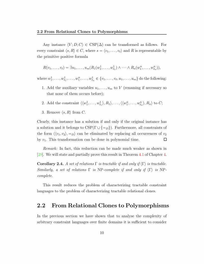

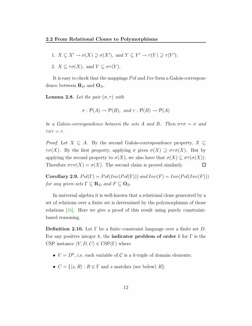


![Datalog: Bag Semantics via Set Semantics - arXiv · Datalog±share these properties: for instance, guarded [8], sticky and weakly-sticky [11] Datalog ± only allow restricted forms](https://static.documents.pub/doc/80x56/5e7e36effe39a8678f12fd4f/datalog-bag-semantics-via-set-semantics-arxiv-datalogshare-these-properties.jpg)
