The concertina pattern: A bifurcation in ferromagnetic thin films Rub´ en Cantero– ´ Alvarez, Felix Otto, Jutta Steiner * August 28, 2006 Abstract The concertina pattern is a metastable stage in the switching process of elongated thin– film elements. It is an approximately periodic structure of domains, separated by walls perpendicular to the long axis of the element. In this paper, we give arguments in favor of our claim that the period is frozen–in at nucleation, i. e. at the critical external field. In prior work, [7, 8], we argued that there are four qualitatively different regimes for nucleation. In one of these asymptotic regimes, the unstable mode displays an oscillatory behavior in direction of the long axis. In this work, we derive a scaling limit of the micromagnetic energy near the bifurcation point in the above regime. We also prove that the scaling limit is coercive for all values of the reduced external field. Because of this coercivity, there exists a branch of non–trivial local minimizers. Numerical minimization of the scaling limit reveals that this branch is indeed a continuous branch of concertina pattern. The scaling limit is derived by Γ–convergence of the suitably rescaled micromagnetic en- ergy. This robust procedure combines the limit of an asymptotic parameter regime with a zoom–in in configuration space. The coercivity of the scaling limit is derived by suitable non–linear interpolation estimates. Mathematics Subject Classification: 78A99, 49K20, 74G60 1 Introduction 1.1 Motivation The micromagnetics of ferromagnetic thin–film elements is a paradigm for a multi- scale pattern–forming system. On one hand, there is a material length scale which is the effective range of the attractive spin–spin interaction (5 nm for Permalloy). On the other hand, there are the sample dimensions (thicknesses typically hundreds * Institute of Applied Mathematics, University of Bonn, Germany 1
Transcript
The concertina pattern: A bifurcation in
ferromagnetic thin films
Ruben Cantero–Alvarez, Felix Otto, Jutta Steiner ∗
August 28, 2006
Abstract
The concertina pattern is a metastable stage in the switching process of elongated thin–
film elements. It is an approximately periodic structure of domains, separated by walls
perpendicular to the long axis of the element. In this paper, we give arguments in favor
of our claim that the period is frozen–in at nucleation, i. e. at the critical external field.
In prior work, [7, 8], we argued that there are four qualitatively different regimes for
nucleation. In one of these asymptotic regimes, the unstable mode displays an oscillatory
behavior in direction of the long axis. In this work, we derive a scaling limit of the
micromagnetic energy near the bifurcation point in the above regime. We also prove that
the scaling limit is coercive for all values of the reduced external field. Because of this
coercivity, there exists a branch of non–trivial local minimizers. Numerical minimization
of the scaling limit reveals that this branch is indeed a continuous branch of concertina
pattern.
The scaling limit is derived by Γ–convergence of the suitably rescaled micromagnetic en-
ergy. This robust procedure combines the limit of an asymptotic parameter regime with a
zoom–in in configuration space. The coercivity of the scaling limit is derived by suitable
The micromagnetics of ferromagnetic thin–film elements is a paradigm for a multi-scale pattern–forming system. On one hand, there is a material length scale whichis the effective range of the attractive spin–spin interaction (5 nm for Permalloy).On the other hand, there are the sample dimensions (thicknesses typically hundreds
∗Institute of Applied Mathematics, University of Bonn, Germany
1
of nm, widths typically several µm). Furthermore there is a long–range spin–spininteraction expressed by the stray field.
There is a well–accepted continuum model for the magnetization m(x) for tempera-tures well below the Curie temperature. In its static version it comes as a variationalproblem for m. In recent years, several reduced models, suited for specific thin–filmregimes, have been derived. They have been derived based on scale separation,within the framework of Γ–convergence [13, 9, 16]. This means that they are rele-vant for ground states and metastable states with energies close to the ground stateenergy.
For the technologically important switching under external fields, however, meta–stable states with energies far from the ground state are important. In a certainsense, an external field probes the complex energy landscape with its many wells.In the case of small samples, all stationary points of the energy have recently beenmapped numerically [10].
For soft (i. e. low crystalline anisotropy) materials, it is the sample shape whichenforces a discrete set of ground states. For an elongated thin–film element forinstance, the two magnetizations in direction of the long axis are favored. Theubiquitous concertina pattern, cf. Figure 1, can be seen as a metastable state in thecascade of events on the road to switching.
Figure 1: The concertina pattern
Figure 1 shows such a pattern seen from above for an elongated Permalloy thin–filmelement of 300nm thickness and 18µm width. The concertina pattern is the almostperiodic microstructure in the center of the element’s cross–section. It is formed bystripe–like domains separated by low–angle Neel walls. Figure 2 gives more insightinto the experimental picture. On the left, the sample and the original ground stateare sketched. Note that for a thin film it can be assumed that the magnetization isessentially in–plane and independent of the thickness direction x3. In particular, theinformation received from the surface can be assumed as valid throughout the wholethickness of the sample. This reduces the problem of a graphical representation to atwo dimensional one, which can be solved by a grey–shade color coding. The middlepicture shows how the color coding has to be interpreted. Increasing scales of greycorrespond to an increasing opacity of the sample sections with respect to polarizedlight. The polarization information itself corresponds with the magnetization of thesample, which lives on the unit circle. Finally, the sharp transitions between theshaded regions show that the concertina pattern is formed by uniformly magnetized
2
domains, separated by comparatively sharp walls. This is taken up in the rightmostsketch of Figure 2.
m
m2
1
Figure 2: Mesoscopic magnetization
The concertina pattern is experimentally generated as follows, cf. Figure 3: First,the element is saturated along the long axis, then the external field is slowly reduced,eventually reversed. At some field strength, the uniform magnetization buckles intothe concertina pattern.
Hext
Figure 3: How the concertina pattern is generated
A traditional analytical approach to switching is “nucleation” theory. One envisionsa ferromagnetic sample which is saturated by a strong external field. As one reducesthe external field, an instability eventually occurs. The corresponding field is calledthe critical field. This first instability of the saturation branch is called nucleation.This may or may not be related to an irreversible event, i. e. switching, see [17].Whether this is the case, depends on the type of bifurcation.
Mathematically speaking, the critical field is the value of the external field at whichthe Hessian of the micromagnetic energy functional ceases to be positive definite.The degenerate subspace consists of the “unstable modes”. The related eigenvalue
3
problem has been explicitly and completely solved for special geometries like el-lipsoids of revolution [6, 11, 2]. As a consequence of the multiscale nature of theproblem, there are different types of unstable modes, depending on and definingparameter regimes. For instance, for sufficiently small samples, the unstable modecorresponds to a coherent rotation of the magnetization, as in the Stoner–Wohlfarthmodel [18]. For sufficiently large samples, the unstable mode corresponds to a curl-ing of m which does not generate a stray field [6]. A third mode, which correspondsto a buckling of the magnetization, has been found numerically [11]. In [17], hystere-sis simulations show the nucleation of a curling mode via a supercritical pitchforkbifurcation.
In [7, 8], we studied the nucleation problem for a cylindrical geometry which mimicsan elongated thin–film element, cf. Section 1.2.2. In the physics literature, there areonly partial results for cylindrical geometries. In [7], we identify exactly four scalingregimes in the two non–dimensional parameters. One of these regimes displays anoscillatory buckling mode and is novel in the sense that the period of oscillation isdetermined by a subtle interaction of sample geometry and material length scales. Itis therefore tempting to make the following hypothesis: The period of the concertinapattern is the frozen–in period of the oscillatory buckling mode discovered in [7].It is noteworthy that this thin–film buckling regime stretches over a wide range inparameter space. This is in contrast with Aharoni’s claim that buckling plays onlya minor role [2, p. 202].
In the companion paper, [8], we asymptotically identify the unstable mode in theoscillatory buckling regime. This is done by identifying the Γ–limit of the Rayleighquotient of the Hessian. We so obtain an asymptotic expression for the period ofoscillation of the unstable mode in terms of the thickness t and width ` of the sample.This expression is consistent with the experimentally observed trends, see Figures 4and 5: The width of the domains in the concertina pattern increases for increasingsample width ` while it decreases for increasing sample thickness t.
Figure 4: Concertina pattern for different widths
In this third paper, we go beyond nucleation and identify a scaling limit of themicromagnetic energy near the critical field. More precisely, we combine the above-mentioned scaling regime with a zoom in on the bifurcation point in configurationspace. This is done by Γ–convergence after suitable renormalization. We show that
4
Figure 5: Concertina pattern for different thicknesses
the scaling limit is coercive for all values of the external field in the reduced set-ting, which yields the existence of a branch of concertina–type minimizers not farin energy from the original global minimizer.
It has to be emphasized that the concertina pattern is not a ground state but ametastable state and, as such, not a global minimizer of the energy functional,but merely a local one. Experimental evidence for this fact is given by coarseningphenomena, as seen in Figure 6. The concertina pattern for one fixed sample isshown in two stages of its development. In the second stage the domain structurehas coarsened by fusion of different domains. This effect may explain the deviationof a factor of two between the period of oscillation of the unstable mode and theexperimental results, see Table 1.
Figure 6: Coarsening of the concertina pattern
Let us now give a short synopsis of this paper’s content. In Subsection 1.2, weintroduce the micromagnetic energy functional and the idealized sample geometry.In Subsection 1.3, we recall the basics of nucleation theory. In Subsection 1.4 and1.5, we review the results of [7] and [8], respectively. Section 2 presents the resultsof this paper. The final section is devoted to the proofs.
1.2 The micromagnetic model
1.2.1 Energy functional
Our analysis is based on the micromagnetic model. Let Ω ⊂ R3 describe the sam-ple geometry. The micromagnetic model states that an experimentally observed
Table 1: Comparison of theory (see [8]) and experiment
magnetization m : Ω → R3 is a local minimum of the micromagnetic energy
E(m) = d2
∫
Ω
|∇m|2 dx (1)
+
∫
R3
|∇um|2 dx (2)
− 2
∫
Ω
Hext · m dx (3)
among all m which satisfy the saturation constraint
|m|2 = 1 in Ω. (4)
This version of the model is partially non–dimensionalized: The magnetization m,the external field Hext, the stray field −∇um, and the energy density are non–dimensional. Length on the other hand is dimensional.
Contribution (1) is the exchange energy, which is of quantum mechanical origin; dis the exchange length, a material parameter. Contribution (2) is the energy of thestray field −∇um. The stray field is determined by the static version of Maxwell’sequations. They are conveniently stated in a distributional form:
∫
R3
∇um · ∇ϕ dx =
∫
Ω
m · ∇ϕ dx for all test functions ϕ. (5)
As can be seen from (5), there are two types of “magnetic charges” which give riseto a stray field:
volume charges −∇ · m in Ω,surface charges ν · m on ∂Ω.
Contribution (3) is the Zeeman term which models the interaction with the externalfield Hext.
6
1.2.2 An idealized geometry
Motivated by the concertina pattern we consider the following idealized samplegeometry
Ω = R × (0, `) × (0, t) with ` t,
see Figure 7. The reasons for this choice are:
• Ω mimics an elongated thin–film element of thickness t and width `. In Section2.1, a finite periodicity L in direction x1 will be imposed.
• Due to the translation invariance in x1, Ω admits m∗ = (1, 0, 0) as a stationarypoint for all external fields of the form Hext = (−hext, 0, 0), hext ∈ R (note thechange of sign), and for an easy axis in direction of x1 or perpendicular to x1.In fact, we shall neglect crystalline anisotropy altogether without much loss ofgenerality.
t
l
x3
x2
x1
Figure 7: The geometry
1.3 Nucleation theory
1.3.1 The Hessian
The local stability of the stationary point m∗ = (1, 0, 0) is described by the secondvariation of the energy E, its Hessian. Due to the constraint |m|2 = 1, infinitesimalperturbations of m∗ = (1, 0, 0) are of the form
δm = (0, δm2, δm3), δm = δm(x1, x2, x3).
The Hessian HessE(m∗) in m∗ is given by
12HessE(m∗)(δm, δm) = 1
2HessE0(m∗)(δm, δm) − hext
∫
Ω
|δm|2 dx, (6)
where HessE0(m∗) denotes the Hessian without Zeeman term, i. e.
12HessE0(m∗)(δm, δm) = d2
∫
Ω
|∇ δm|2 dx +
∫
R3
|∇uδm|2 dx,
and the magnetostatic potential uδm is determined by δm in the usual way.
7
Figure 8: Infinitesimal perturbations
1.3.2 Variational characterization of critical field and unstable modes
The critical field hcrit is the value of hext for which HessE(m∗) ceases to be posi-tive definite. The unstable modes are the elements of the degenerate subspace ofHessE(m∗) at hext = hcrit. The following variational characterization of both canbe inferred from (6): hcrit and the (normalized) unstable modes are the minimumand the minimizers, respectively, of the variational problem
12HessE0(m∗)(δm, δm) subject to
∫
Ω
|δm|2 dx = 1. (7)
It is natural to capitalize on the translation invariance of (7) in x1 by a partialFourier transform in that variable. More precisely, the Hessian HessE0(m∗)(·, ·)factorizes into HessE0(m∗)(k1, ·, ·)k1∈R, where
1
2HessE0(m∗)(k1, δm, δm) = d2
∫
(0,`)×(0,t)
(k2
1 |δm|2 + |∂2 δm|2 + |∂3 δm|2)dx2dx3
+
∫
R2
(k2
1 |uδm|2 + |∂2 uδm|2 + |∂3 uδm|2)dx2dx3, (8)
k1 denotes the dual variable to x1 and δm = δm(x2, x3). Hence we replace thevariational problem (7) in δm(x1, x2, x3) by the variational problem in δm(x2, x3)and k1 of minimizing
12HessE0(m∗)(k1, δm, δm) subject to
∫
(0,`)×(0,t)
|δm|2 dx2dx3 = 1. (9)
Notice that unstable modes can also be seen as the ground states for the operator
L δm = −d24Neumannδm −(
∂2
∂3
)uδm. (10)
A complete explicit diagonalization beyond the obvious factorization (8) of L seemsnot at hand. Indeed, the contribution from the exchange energy is diagonal w. r. t.cosine series in (x2, x3) whereas the contribution from the magnetostatic energy isdiagonal w. r. t. the Fourier transform in (x2, x3). This lack of compatibility reflectsthe fact that the exchange energy is confined to the sample but the energy of thestray field extends into the ambient space.
8
1.4 Identification of four scaling regimes
A rigorous analysis of the scaling of the critical field hcrit was carried out in [7]. Bydimensional analysis, hcrit is a function of the non–dimensional parameters t/d, `/d:
hcrit = hcrit(t/d, `/d). (11)
In [7], all regimes for the scaling of this function are identified:
Theorem 1. [7] There exists a universal constant C < ∞, s. t. for t ≤ 1C
`:
1
Chcrit. ≤
t`ln(
`t
)for t ≤ d2
`ln−1
(`d
)Regime I
(d`
)2for d2
`ln−1( `
d) ≤ t ≤ d2
`Regime II
(dt`2
)2/3for d2
`≤ t ≤ (d`)1/2 Regime III
(dt
)2for (d`)1/2 ≤ t Regime IV
≤ C hcrit..
(12)
Theorem 1 can best be visualized in terms of a phase diagram for (11) in parameterspace, see Figure 9.
t11
d
I II III IV
d
t/ /t
dt/2/3
l
ll
l2
ln )
((
)
((
/t )2
/l )2
/d
/d
Figure 9: Phase diagram for hcrit(t/d, `/d)
Theorem 1 is proved by establishing upper and lower bounds on (9) which match interms of scaling. The upper bounds stem from physically motivated models. Themain contribution of a mathematically minded analysis is to show that these modelscan not be substantially improved, i. e. in terms of scaling. This is done by providing
9
ansatz–free lower bounds, which rely on suitable interpolation inequalities. In thissense the analysis of [7] is half–way between proposing (new) models and identifyingground–state modes.
1.5 Identification of the unstable mode in Regime III
Theorem 1 identifies all scaling regimes by determining the scaling of hcrit, but itdoes not determine the degenerate subspace. We now present a result from [8] whichrigorously identifies the asymptotic degenerate subspace in the new Regime III.
1.5.1 The scaling
In [8] we identify the asymptotic minimizers (k1, δm2(x2, x3), δm3(x2, x3)) by char-acterizing the Γ–limit of (9). This requires a non–dimensionalization, which will beperformed anisotropically as follows
x1 =
(d2`2
t
)1/3
x1, x2 = ` x2, x3 = t x3, (13)
with the implicit understanding that this also means k1 =(
td2`2
)1/3k1, ∂2 = `−1∂2,
dx2 = ` dx2 and so on. In view of the constraint in (9) we rescale the infinitesimalperturbation as follows
δm = (`t)−1/2 δm.
In view of Theorem 1 and hcrit = 12min HessE0, the Hessian itself has to be rescaled
as
HessE0 =
(dt
`2
)2/3
HessE0.
We finally introduce the two non–dimensional parameters
ε :=
(d2
`t
)2/3
and δ :=
(t2
d`
)2/3
(14)
which characterize Regime III:
ε 1 and δ 1. (15)
1.5.2 The result
Theorem 2. [8] The variational problem of minimizing
12HessE0(m∗)(k1, δm, δm) subject to
∫
(0,`)×(0,t)
|δm|2 dx2dx3 = 1 (16)
Γ–converges in the regime (15) under weak convergence of (k1, δm2, δm3) in R ×L2((0, 1) × (0, 1))2 to the variational problem of minimizing
k21
∫ 1
0
(δm2)2 dx2 +
1
2 |k1|
∫ 1
0
(∂2 δm2)2 dx2 subject to
∫ 1
0
|δm2|2 dx2 = 1 (17)
10
if (δm2, δm3) is of the form (δm2(x2), 0) with δm2 ∈ H10 ((0, 1)), and +∞ if this is
not the case.
The fact that δm2 ∈ H10 ((0, 1)), i. e. that the boundary values are fixed at zero, is
called “edge–pinning”. For the notion of Γ–convergence, we refer to [5, Chapter1.2]. The variational problem (17) can be solved explicitly, as illustrated in Figure10. Edge–pinning fixes the shape of the eigenfunction as a sine in x2 with a multipleof π as wave vector. Minimization in x2 yields sin(πx2), which can be inserted.Subsequent minimization in k1 determines the oscillation wave vector.
sin( x
ω
|kk1*
π
π
|1
2)
2)
sin(2 x
Figure 10: Dispersion relation
The unstable subspace asymptotically consists of all perturbations δm of the form
δm2 = 2(`t)−1/2 cos
(2πx1
w
)sin(πx2
`
)and δm3 ≡ 0. (18)
where the period w = 2 π|k1|
of oscillation in the infinite direction x1 is asymptoticallygiven by
w ≈(
32πd2 `2
t
)1/3
, (19)
which specifies (18).
We return to the hypothesis that the observed period wexp of the concertina patternis the frozen–in length scale (19) of the unstable mode. We have compared wexp
to w for eight experiments pictured in [15]. These experiments cover a substantialrange of the non–dimensional parameters t/d and `/d, see Table 1.
2 Results
We recall our bold claim that the period of the concertina pattern is the frozen–inlength scale of the unstable mode. This claim is only substantiated if there are localminimizers of concertina type close to the critical point m∗ in configuration space.
11
This would be the case if the bifurcation was supercritical — which turns out notto be the case, cf. Subsection 2.2. Despite this fact, we can show that such localminimizers indeed exist near m∗, see Theorem 5 in Subsection 2.2.
Our strategy is the following: We rigorously derive a scaling limit of a suitablyrenormalized energy in Regime III which zooms in near m∗ in configuration space,see Theorem 3 in Subsection 2.1. We then prove that this scaling limit is coercivefor all external fields, see Theorem 4 in Subsection 2.2.
2.1 Scaling limit of the renormalized energy
In this section we renormalize the energy in Regime III and identify a scaling limitwhich includes the dominant nonlinearity. In order to preserve translation invariancewhile working with a finite volume, we impose a convenient periodicity L in theinfinite x1–direction:
m(x1 + L, x2, x3) = m(x1, x2, x3).
This yields a well–defined energy functional E
E(m) = d2
∫
(0,L)×(0,`)×(0,t)
|∇m|2 dx +
∫
(0,L)×R2
|∇um|2 dx
+2hext
∫
(0,L)×(0,`)×(0,t)
m1 dx, (20)
where um inherits the periodicity of m in x1.
In order to find the scaling limit, one zooms in on m∗ in the energy landscape at theright scale. The zooming–in is combined with the asymptotic Regime III, cf. Figure11. This is done in Theorem 3, in the framework of Γ–convergence.
/dt
l/d
III 13/d )t/( 2l~
mm
E
*
Figure 11: Zoom in on m∗
2.1.1 The scaling
Length is non–dimensionalized as for Theorem 2, i. e. (13). The new element is therescaling of the (m2, m3)–components of the magnetization, which we motivate now.
12
Notice that for m ≈ m∗ = (1, 0, 0), (m2, m3) can be seen as the finite version of theinfinitesimal perturbation (δm1, δm2). Remark that
m1 =√
1 − m22 − m2
3 ≈ 1 − 12(m2
2 + m23) for m ≈ (1, 0, 0).
As for Theorem 2 we expect that in Regime III the out–of–plane component isstrongly suppressed by the penalization of surface charges so that the above turnsinto
m1 ≈ 1 − 12m2
2. (21)
The magnetization component m2 will be rescaled in such a way as to balance thetwo contributions to the volume charge distribution ∇ · m, i. e.
The external field is measured in units of the critical field as identified in Theorem1. As for the energy (20) itself, we subtract E(m∗) and normalize appropriately:
hext =
(dt
`2
)2/3
hext, E − 2 hext L ` t =
(d8t2
`
)1/3
E. (23)
We are now left with four non–dimensional parameters, ε, δ from (14) and also Land hext. We are interested in Regime III close to critical field. In order to end upwith a finite volume in the limit, we are forced to assume
L ∼ 1 and likewise hext ∼ 1. (24)
This means that L is of the order of the oscillation period w; we think of L as beinga large, but O(1) multiple of w, where according to (13), L is defined as
L =
(d2`2
t
)1/3
L.
Throughout the analysis, it will be useful to work with the combined Fourier seriesin x1 and Fourier transform in x2, i. e.
F(f)(k′) =1√2πL
∫
(0,L)×R
exp(ik′ · x′) f dx′ for k′ = (k1, k2) ∈2π
LZ × R, (25)
and to introduce the notation∫
2π
LZ×R
dk′ :=∑
k1∈2π
LZ
∫
R
dk2.
13
2.1.2 The limit
Theorem 3. Fix an M ∼ 1. The variational problem of minimizing
E subject to |m|2 = 1 and
∫
(0,L)×(0,1)×(0,1)
|m − m∗|2 dx = εM2 (26)
Γ–converges in the regime described by (15) & (24) under weak convergence for(m2, m3) in L2((0, L) × (0, 1) × (0, 1))2 to the variational problem of minimizing
E0 :=
∫
(0,L)×(0,1)
(∂1m2)2 dx′ + 1
2
∫
(0,L)×R
∣∣|∂1|−1/2(− ∂1(
12m2
2) + ∂2m2
)∣∣2 dx′
−hext
∫
(0,L)×(0,1)
m22 dx′ subject to
∫
(0,L)×(0,1)
m22 dx′ = M2 (27)
if (m2, m3) is of the form (m2(x′), 0) and E0 = +∞ if it is not of this form.
Here |∂1|−1/2 denotes the operator with Fourier symbol |k1|−1/2. The expression−∂1(
12m2
2) + ∂2m2 is to be understood distributionally where m2 is zero outside ofR × (0, `). As for Theorem 2, this imposes edge–pinning, i. e. m2(x2=1) = m2(x2=0) = 0 in a weak sense.
Let us point out that E0 interpolates between a linear regime and a highly nonlinearwall regime.
• For dominant ∂2m2, E0 is close to the Γ–limit (17) of the Hessian integratedover frequencies k1:
E0 ≈∫
2π
LZ
(k2
1
∫ 1
0
m22 dx2 +
1
2|k1|
∫ 1
0
(∂2m2)2 dx2 − hext
∫ 1
0
m22 dx2
)dk1,
thus, this is expected to be a good description near the bifurcation.
• For dominant −∂1(12m2
2), E0 is close to a 1–d model for small–angle thin–filmNeel walls (“ripples”) normal to x1, integrated over x2:
E0 ≈∫ 1
0
(∫ L
0
(∂1m2)2 dx1 +
1
2
∫ L
0
∣∣|∂1|1/2(12m2
2)∣∣2 dx1 − hext
∫ L
0
m22 dx1
)dx2.
(28)This picture closely corresponds to the theory of magnetic domains and isexpected to describe the situation for external fields large in this scale.
2.1.3 Numerical simulations
For the definition of a discrete energy functional Eh0 , we use a discrete approximation
of the magnetization on an equidistant grid. The discretization is straightforwardin the case of the exchange and Zeeman contributions via finite differences and
14
quadrature. The stray–field contribution involves a nonlocal expression (in x1–direction) of the nonlinear charge density
σ := −∂1
(1
2m2
2
)+ ∂2 m2.
A discrete charge density can be defined by discrete differences. The nonlocalityimpels us to use the Fast Fourier Transform for reasons of complexity. Thus, weneed to calculate the discrete Fourier multiplier. We recall that the stray–field termcan be expressed by the Dirichlet integral of a harmonic extension U into the half–space R × x3 > 0, where [
∂U
∂x3
] ∣∣∣x3=0
= σ.
The elliptic problem can be discretized in the usual way in x1–direction. The Fourierrepresentation of the solution then yields the correct discrete multiplier.
For hext > hcrit, minimization of Eh0 is performed by means of a generalized descent
algorithm. The directions of descent are calculated via an inexact Newton method,the resulting linear system is solved by a conjugate gradient method. In order tocalculate a good initial value at a certain h0
ext > hcrit, Eh0 is first minimized on the
two–dimensional subspace 〈m+2 , m++
2 〉, where m+2 , m++
2 are the discrete versions ofthe modes given in Subsection 2.2.1. The minimizer so obtained can then be usedas an initial value for nearby values hext > h0
ext.
Numerical simulation of E0 reveals a branch of solutions which turn into the con-certina pattern as the critical field is increased, see Figure 12. L was choosen to bean integer multiple of the theoretically predicted period (3 in the present case). Thefigure displays the pattern at external field values of hext = 5.4723, hext = 9.6653,and hext = 18.6914. The figure displays m2 by a gray scale plot.
Figure 12: A continuous branch of minimizers of the scaling limit
The numerical results show a branch of non–trivial minimizers of concertina type.Note that the three selected figures show a transition from a pattern close to thebifurcation mainly determined by the two modes m+
2 , m++2 , cf. Subsection 2.2.1, to
a pattern with a strict lengthscale separation between domain and wall width.
15
2.2 Existence of non–trivial local minimizers
2.2.1 A subcritical bifurcation
A straightforward approach to ascertain the existence of non–trivial local minimizersis the use of bifurcation theory. Classically, one distinguishes between a subcritical, atranscritical and a supercritical bifurcation, see Figure 13. We shall now argue on thelevel of the scaling limit E0 that the bifurcation is subcritical. Hence the traditionalbifurcation theory will not yield the existence of non–trivial local minimizers.
hcrithext
hcrit
hexthcrit
hext
Figure 13: Sub–, trans, and supercritical bifurcation
Neglecting the hats, the scaling limit can be rewritten as:
E0(m2) =1
2〈m2,Lm2〉 + N3(m2, m2, m2) + N4(m2, m2, m2, m2)
−hext
∫ 1
0
∫ L
0
m22 dx1 dx2,
where
1
2〈m2,Lm2〉 =
∫ 1
0
∫ L
0
[(∂1m2)
2 +1
2
∣∣|∂1|−1/2∂2m2
∣∣2 − hcrit m22
]dx1 dx2 (29)
N3(m2, m2, m2) = −∫ 1
0
∫ L
0
|∂1|−1/2∂2m2 |∂1|−1/2∂1(12m2
2) dx1 dx2
N4(m2, m2, m2, m2) =1
2
∫ 1
0
∫ L
0
∣∣|∂1|−1/2∂1(12m2
2)∣∣2 dx1 dx2.
The linear operator L defined by the bilinear form (29) corresponds to the Γ–limit ofthe Hessian for the critical external field, integrated in x1. Thus, it has the followingproperties:
L ≥ 0 and ker L = 〈 cos(k1 x1) sin(πx2) 〉 =: 〈m+2 〉,
cf. Theorem 2. For an asymptotic expansion, the contributions of lowest order to E0
restricted on the one–dimensional kernel of L, t m+2 |t ∈ R, have to be calculated.
It turns out that by symmetry
N3(m+2 , m+
2 , m+2 ) = 0.
16
As the cubic term degenerates on ker L, one has to include a perturbation of higherorder in the asymptotic analysis, thus the ansatz is to restrict E0 onto t m+
2 +t2 m++
2 |t ∈ R, to neglect all terms o(t4) and to minimize in m++2 . This leads to an
Euler–Lagrange equation for m++2 , by variation
∀ζ : 0 = 〈ζ,Lm++2 〉 +
(N3(ζ, m+
2 , m+2 ) + N3(m
+2 , ζ, m+
2 ) + N3(m+2 , m+
2 , ζ)).
Integration by parts yields
0 = −2∂21m
++2 − |∂1|−1∂2
2m++2 − 2 hcrit m
++2
+|∂1|−1∂2∂1(12(m+
2 )2) + (∂1∂2|∂1|−1m+2 )m+
2
= −2∂21m
++2 − |∂1|−1∂2
2m++2 − 2 hcrit m
++2 − π
2sin(2k1x1) sin(2πx2).
The solution is given by
m++2 =
1
10
(2
π
)1/3
sin(2k1x1) sin(2πx2).
Thus, the behavior of E0 at the critical field in fourth order is given by
E0(tm+2 + t2m++
2 ) =(− 1
2〈m++
2 ,Lm++2 〉 + N4(m
+2 , m+
2 , m+2 , m+
2 ))
t4 + O(t5)
=(− π
40+
3π
128
)t4 + O(t5)
= − π
640t4 + O(t5). (30)
Because of the negative quartic term in the energy, the bifurcation is subcritical.This is due to cancellations of the charge density σ in the small. In fact, thesecondary mode m++ lowers the energy, see Figure 14. Though the exchange energyrises by the new spectral component, the charges are moved closer together, s. t. thestray–field contribution is lowered. The second effect is stronger than the first one,yielding a lower energy.
2.2.2 Coercivity
Since the straightforward bifurcation argument fails to yield the existence of localminimizers, we take another approach: We will establish the coercivity of E0 for allvalues of hext. This yields the existence of non–trivial local minimizers for hext ≥ hcrit
which carries over to E.
Coercivity is called into question by cancellations in the charge density
σ := −∂1
(1
2m2
2
)+ ∂2 m2.
Note that σ vanishes for all weak solutions of Burgers’ equation (with x2 playing therole of time and −x1 that of space). Hence, there is the possibility that the quartic
17
0 L
1
0 L
1
Unstable mode, t=1 Both modes, t=1
Figure 14: Improved dipolar charge screening
term in E0 is ineffective in ensuring coercivity. In fact, the previous subcriticalityresult is a consequence of charge cancellations in the small. The following theoremshows that there are no cancellations in the large, though.
Theorem 4. There exists a universal constant C < ∞ such that for any m2 ∈L2((0, L) × (0, 1)) we have
E0(m2) ≥ 1
CL−5/3
(∫
(0,L)×(0,1)
m22 dx′
)14/9
− hext
∫
(0,L)×(0,1)
m22 dx′.
It is not claimed that the exponent 14/9 is optimal; it is just important that it islarger than 1.
The expected shape of the bifurcation and the corresponding impressions of theenergy landscape are pictured in Figure 15.This is indeed confirmed by numerical simulation via an explicit reparametrization,see Figure 16.
For fields smaller than the field at the turning point — where the dashed curvemeets the full curve — there is only one minimizer m∗. At the turning point, theenergy landscape becomes more complicated, as two further local minimizers ±m0
appear. This does not influence m∗ yet, which is still a local minimizer until hcrit isreached. At hcrit, the minimizer m∗ is completely destabilized. For fields larger thanhcrit, m∗ is a local maximizer and the local minimizers ±m0 evolve into concertinapattern.
2.2.3 Existence
We know that the reduced Γ–limit E0 of E experiences a subcritical bifurcation andis coercive. Combining both results, we arrive at
Theorem 5. Let regimes (15) & (24) be true. Then there exists a constant C < ∞s. t. for all hext ≥ hcrit − 1
Cthere exists an m0 s. t.
18
h ext
1/22m2
E
h
m2
crit
Figure 15: Shape of the bifurcation
• m0 6= m∗
• m0 is a local minimizer of E w. r. t. the L2((0, L), (0, 1), (0, 1))–topology
•∫(0,L)×(0,1)×(0,1)
|m0 − m∗|2 dx ≤ Cε.
3 Proofs
The proofs are organized as follows: Subsections 3.1 and 3.2 focus on the lowersemicontinuity part of the Γ–convergence result. In Subsection 3.1, the necessarycompactness result is established, followed by the lower semicontinuity argumentin Subsection 3.2. The next two sections deal with the construction of a recoverysequence. Central to the construction is the use of smooth functions, justified byan approximation result in Subsection 3.3. The construction itself is performed inSubsection 3.4. The last Subsection contains the proofs of Theorem 4 and Theorem5.
Before starting with the proofs, let us introduce the notation f . g. By thiswe qualify expressions whose ratio f/g is bounded from above by a nonnegativeconstant independent of the parameters in question, e. g. ε and δ.
3.1 Compactness
In this section, we establish a compactness result necessary for the proof of the lowersemicontinuity part of the Γ–convergence. We introduce the vertical average of a
19
0
0.5
1
1.5
2
2.5
3
3.5
^ ^1.01*hcrit hcrit
22
1/2
field
<m >
external
Figure 16: Numerical results
quantity f :
〈f〉 =1
t
∫ t
0
f dx3 =
∫ 1
0
f dx3.
Proposition 1. Let the sequences ενν↑∞, δνν↑∞ converge to zero. Let L, hext begiven. Consider a sequence mν : R3 7→ S2ν↑∞ of vector fields which are L–periodicin x1, supported in x2 ∈ [0, `ν], x3 ∈ [0, tν], such that
1
εν
∫
(0,L)×(0,1)×(0,1)
|mν − m∗|2 dx, E(mν) bounded for ν ↑ ∞. (31)
Then
limν↑∞
1
εν
∫
(0,L)×(0,1)×(0,1)
|mν − (1, 〈m2〉, 〈m3〉)|2 dx = 0, (32)
limν↑∞
∫
(0,L)×(0,1)
〈mν,3〉2 dx′ = 0, (33)
〈mν,2〉ν↑∞ is compact in L2((0, L) × (0, 1)). (34)
The first lemma shows that the exchange energy is strong enough to slave m to(1, 〈m2〉, 〈m3〉) in the L2–topology. It proves part (32) of Proposition 1.
Lemma 1. In regime (15),∫
(0,L)×(0,1)×(0,1)
|m − m∗|2 dx . ε and E . 1 (35)
20
imply ∫
(0,L)×(0,1)×(0,1)
|m − (1, 〈m2〉, 〈m3〉)|2 dx . ε3/2 + δ2ε. (36)
Proof of Lemma 1. For notational convenience, we write∫
dx for the integral∫(0,L)×(0,1)×(0,1)
dx and∫
dx′ for∫(0,L)×(0,1)
dx′. We start by observing
∣∣∣∣hext
∫ε−1(m1 − 1) dx
∣∣∣∣ . 1. (37)
Indeed, since hext ∼ 1, cf. (24), it suffices to show∫|m1−1| dx . ε. To this purpose,
we observe that due to |m|2 = 1,
|m1 − 1|
= 1 −√
1 − m22 − m2
3 ≤ m22 + m2
3 for m1 ≥ 0≤ (m1 − 1)2 for m1 ≤ 0
and thus by assumption (35)
∫|m1 − 1| dx ≤
∫|m − m∗|2 dx . ε.
This establishes (37).
We now argue that∫
|∂1m|2 dx . ε,
∫|∂2m|2 dx . 1,
∫|∂3m|2 dx . δ2ε. (38)
Indeed, neglecting the non–negative magnetostatic energy we find after rescalingaccording to (13)&(23)
E ≥∫
ε−1|∂1m|2 + |∂2m|2 + δ−2ε−1 |∂3m|2 dx + 2hext
∫ε−1(m1 − 1) dx.
Now (38) follows from (37) and our assumption E . 1, cf. (35).
We now establish that ∫〈m2〉4 + 〈m3〉4 dx′ . ε3/2. (39)
We only treat the m2–component, since the argument for m3 is identical. We remarkthat (39) follows from (38) in its x3–averaged form, i. e.
∫(∂1〈m2〉)2 dx′ ≤
∫(∂1m2)
2 dx . ε,∫
(∂2〈m2〉)2 dx′ ≤∫
(∂2m2)2 dx . 1,
and ∫〈m2〉2 dx′ ≤
∫m2
2 dx(35)
. ε
21
via the interpolation estimate∫〈m2〉4 dx′ .
(∫(∂1〈m2〉)2 dx′ +
∫〈m2〉2 dx′
)
×(
ε1/2
∫(∂2〈m2〉)2 dx′ + ε−1/2
∫〈m2〉2 dx′
). (40)
The interpolation estimate (40) is easily established. We start with
∫〈m2〉4 dx′ ≤
∫ 1
0
supx1
〈m2〉2 dx2
∫ L
0
supx2
〈m2〉2 dx1. (41)
On the one hand for fixed x1, the following estimate on the unit length intervalx2 ∈ [0, 1] holds for all ε . 1:
supx2
〈m2〉2 . ε1/2
∫ 1
0
(∂2〈m2〉)2 dx2 + ε−1/2
∫ 1
0
〈m2〉2 dx2,
and thus
∫ L
0
supx2
〈m2〉2 dx1 . ε1/2
∫(∂2〈m2〉)2 dx′ + ε−1/2
∫〈m2〉2 dx′. (42)
On the other hand, since L ∼ 1, cf. (24), we have for fixed x2
supx1
〈m2〉2 .∫ L
0
(∂1〈m2〉)2 dx1 +
∫ L
0
〈m2〉2 dx1
and thus ∫ 1
0
supx1
〈m2〉2 dx2 .
∫(∂1〈m2〉)2 dx′ +
∫〈m2〉2 dx′. (43)
The interpolation inequality (40) now follows from inserting (42)&(43) into (41).
We now argue that (36) holds at least where m1 is non–negative:∫
so that (45) is a consequence of (39), i. e.∫〈m2〉4 dx′ . ε3/2 and (38), via Poincare’s
estimate in x3 ∈ [0, 1],
∫(m2 − 〈m2〉)2 dx′ .
∫(∂3m2)
2 dx . δ2ε.
Finally, we shall turn to the missing term in (44):
∫
m1≤0
(1 − m1)2 dx . ε3/2 + δ2 ε. (46)
Obviously, (36) is just the sum of (44) and (46). To establish (46), we choose asmooth function η = η(〈m1〉) with the property
η = 1 for 〈m1〉 ≤ 1
4and η = 0 for 〈m1〉 ≥ 1
2. (47)
Notice that we have for the 2–d Lebesgue measure w. r. t. x:
L2(supp η(〈m1〉)
) (47)
≤ L2(〈m1〉 <
1
2)
.
∫(1 − 〈m1〉)2 dx′
≤∫
(1 − m1)2 dx
(35)
. ε 1.
Hence we have by Sobolev–Poincare’s inequality, [14],
∫η(〈m1〉)2 dx′ .
(∫|∇′η(〈m1〉)| dx′
)2
≤∫
η′(〈m1〉)2 dx1
∫|∇′〈m1〉|2 dx′, (48)
where η′ denotes the derivative of η w. r. t. 〈m1〉. According to (38),
∫|∇′〈m1〉|2 dx′ ≤
∫(∂1m1)
2 + (∂2m1)2 dx . 1.
Furthermore, we have on the one hand
∫η(〈m1〉)2 dx′
(47)
≥ L2(〈m1〉 ≤
1
4)
and on the other hand
∫η′(〈m1〉)2 dx′
(47)
. L2(1
4≤ 〈m1〉 ≤
1
2),
23
so that (48) turns into
L2(〈m1〉 ≤
1
4). L2
(1
4≤ 〈m1〉 ≤
1
2). (49)
We first estimate the r. h. s. of (49) by Poincare’s estimate in x2 ∈ [0, 1]
L2(1
4≤ 〈m1〉 ≤
1
2)
. L3(0 ≤ m1 ≤
3
4)
+
∫(m1 − 〈m1〉)2 dx
.
∫
m1 ≥ 0
(m1 − 1)2 dx +
∫(∂3 m1)
2 dx
(44),(38)
. ε3/2 + δ2 ε (50)
We now address the l. h. s. of (49):
∫
m1≤0
(1 − m1)2 dx . L3
(m1 ≤ 0
)
. L2(〈m1〉 ≤
1
4)
+
∫(m1 − 〈m1〉)2 dx
. L2(〈m1〉 ≤
1
4)
+
∫(∂3m1)
2 dx
(38)
. L2(〈m1〉 ≤
1
4)
+ δ2ε. (51)
Finally, (51), (49) & (50) yield (46).
We now turn to the magnetostatic energy. We evoke a result from [8, Lemma 1],which gives a lower bound in terms of the vertically averaged, in–plane divergence
σ′ := ∂1〈m1〉 + ∂2〈m2〉.
In fact, we need a minor modification of [8, Lemma 1], whose proof is given for thereader’s convenience.
Lemma 2.∫
(0,L)×R2
|∇um|2 dx
≥ t3∫
2π
LZ×R
1
2 t|k′| + (t|k′|)2|F(σ′)|2 dk′
+t
∫
2π
LZ×R
1
1 + 12t|k′| + 1
12(t|k′|)2
∣∣F(〈m3〉) − ik′ · F(〈(x3 − t
2)m′〉
)|2 dk′. (52)
24
Proof of Lemma 2. It is convenient to shift the sample from 0 < x3 < t to− t
2< x3 < t
2 and to non–dimensionalize all length in units of t (no hats). We
will actually show that for any vector field m supported in − 12
< x3 < 12 and
L–periodic in x1 we have
minm3
∫
(0,L)×R2
|∇um|2 dx∣∣∣m′ given, 〈m3〉 given
=
∫
2π
LZ×R
|F(σ′)|22|k′| + |k′|2 dk′ +
∫
2π
LZ×R
|F(〈m3〉) − ik′ · F(〈x3m′〉)|2
1 + 12|k′| + 1
12|k′|2 dk′. (53)
Notice that this implies (52). We first notice that (53) can be written as a saddlepoint problem. This is a consequence of the following representation of the strayfield energy:
∫
(0,L)×R2
|∇um|2 dx
= maxv
−∫
(0,L)×R2
|∇v|2 dx + 2
∫
(0,L)×R2
∇v · m dx
.
The first variation w. r. t. m3 yields
∂23um = 0 for x3 ∈ (−1
2, 1
2). (54)
Notice that since the average 〈m3〉 of m3 in x3 is prescribed, it is only the secondderivative ∂2
3um w. r. t. x3 which vanishes and not the first. The first variation w. r. t.v yields
∆um = 0 for x3 6∈ (−12, 1
2),
∆um = ∇ · m for x3 ∈ (−12, 1
2),
∂3um(x′, 12+) − ∂3um(x′, 1
2−) = −m3(x
′, 12) for x3 = 1
2,
∂3um(x′,−12+) − ∂3um(x′,−1
2−) = m3(x
′,−12) for x3 = 1
2.
We take the Fourier transform in x′ and obtain by use of (54):
−|k′|2F(um) + ∂23F(um) = 0 for x3 6∈ (−1
2, 1
2), (55)
−|k′|2F(um) = F(∇ · m) for x3 ∈ (−12, 1
2), (56)
∂3F(um)(k′, 12+) − ∂3F(um)(k′, 1
2−) = −F(m3)(k
′, 12) for x3 = 1
2, (57)
∂3F(um)(k′,−12+) − ∂3F(um)(k′,−1
2−) = F(m3)(k
′,−12) for x3 = 1
2. (58)
In view of (54) and (55), F(um) must be of the form
F(um)(k′, x3) = u(k′) ×
exp((12− x3)|k′|) 1
2≤ x3
1 −12≤ x3 ≤ 1
2
exp((12
+ x3)|k′|) x3 ≤ −12
+ v(k′) ×
12
exp((12− x3)|k′|) 1
2≤ x3
x3 −12≤ x3 ≤ 1
2
−12
exp((12
+ x3)|k′|) x3 ≤ −12
. (59)
25
Because of
∂3F(um)(k′, x3) = u(k′) ×
−|k′| exp((12− x3)|k′|) 1
2≤ x3
0 −12≤ x3 ≤ 1
2
|k′| exp((12
+ x3)|k′|) x3 ≤ −12
+ v(k′) ×
−12|k′| exp((1
2− x3)|k′|) 1
2≤ x3
1 −12≤ x3 ≤ 1
2
−12|k′| exp((1
2+ x3)|k′|) x3 ≤ −1
2
,(60)
(57) & (58) turn into
F(m3)(k′, 1
2) = |k′| u(k′) + (1 + 1
2|k′|)v(k′),
F(m3)(k′,−1
2) = −|k′| u(k′) + (1 + 1
2|k′|)v(k′).
(61)
We now determine u and v. To this aim, we consider (56) which in view of (59)turns into
−|k′|2 (u(k′) + v(k′) x3) = F(∇ · m). (62)
For u, we take the average in x3 ∈(−1
2, 1
2
)of (62):
−|k′|2u(k′) = F(σ′)(k′) +(F(m3)(k
′, 12) − F(m3)(k
′,−12))
(61)= F(σ′)(k′) + 2|k′|u(k′),
yielding
u(k′) = − F(σ′)(k′)
2|k′| + |k′|2 . (63)
For v, we multiply (62) with x3 and take the average in x3:
− 112|k′|2 v(k′) = −〈x2
3〉 |k′|2 v(k′)
= F(〈x3∇′ · m′〉)(k′) + F(〈 x3 ∂3m3〉)(k′)
= ik′ · F(〈x3m′〉)(k′) − F(〈m3〉)(k′)
+12
(F(m3)(k
′, 12) + F(m3)(k
′,−12))
(61)= ik′ · F(〈x3m
′〉)(k′) − F(〈m3〉)(k′) + (1 + 12|k′|) v(k′),
yielding
v(k′) =−ik′ · F(〈x3m
′〉)(k′) + F(〈m3〉)(k′)
1 + 12|k′| + 1
12|k′|2 . (64)
Hence we obtain by Plancherel (mixed terms vanish because of different symmetry
26
in x3)
∫
(0,L)×R2
|∇um|2 dx
=
∫
2π
LZ×R
∫
R
(|k′|2|F(um)|2 + |∂3F(um)|2
)dx3 dk′
(59),(60)=
∫
2π
LZ×R
|u|2(|k′|2 + 2|k′|
)dk′ +
∫
2π
LZ×R
|v|2(1 + 1
2|k′| + 1
12|k′|2
)dk′
(63),(64)=
∫
2π
LZ×R
|F(σ′)|22|k′| + |k′|2 dk′ +
∫
2π
LZ×R
|F(〈m3〉) − ik′ · F(〈x3m′〉)|2
1 + 12|k′| + 1
12|k′|2 dk′.
The following lemma shows that the magnetostatic energy (in conjunction withexchange) is strong enough to suppress the m3–component to leading order. Incombination with Lemma 1, Lemma 3 shows that m is slaved to 〈m2〉. Lemma 3 isa variant of [8, Lemma2]. It proves part (33) of Proposition 1.
Lemma 3. In regime (15),
∫
(0,L)×(0,1)×(0,1)
|m − m∗|2 dx . ε and E . 1
imply ∫
(0,L)×(0,1)
〈m3〉2 dx′ . δ2 + ε δ.
Proof of Lemma 3. We start by observing that because of t ` we have
t
∫
(0,L)×(0,`)
〈m3〉2 dx′
. t
∫
t|k2|≤1
|F(〈m3〉)|2 dk′ + t3∫
(0,L)×(0,`)
(∂2〈m3〉)2 dx′. (65)
For a proof of this elementary estimate (65) we refer to [7, Lemma 5]. The secondterm in (65) can be estimated via Cauchy–Schwarz in x3 by the full exchange energy:
t3∫
(0,L)×(0,`)
(∂2〈m3〉)2 dx′ ≤(
t
d
)2
d2
∫
(0,L)×(0,`)×(0,t)
|∇m|2 dx. (66)
For the first term in (65), we appeal to the elementary Fourier multiplier estimate
1 . min1, 1
t2|k′|2 + t2 k21 for t|k2| ≤ 1, (67)
27
cf. [7, Lemma 7]. Thanks to (67) we have
t
∫
t|k2|≤1
|F(〈m3〉)|2 dk′ . t
∫
2π
LZ×R
min1, 1
t2|k′|2 |F(〈m3〉)|2 dk′
+t3∫
(0,L)×(0,`)
(∂1〈m3〉)2 dx′. (68)
For the last term in (68) we appeal once more to Cauchy–Schwarz
t3∫
(0,L)×(0,`)
(∂1〈m3〉)2 dx′ ≤(
t
d
)2
d2
∫
(0,L)×(0,`)×(0,t)
|∇m|2 dx. (69)
We now turn to the first r. h. s. term of (68). To this purpose, we appeal to Lemma2, which yields in particular
t
∫
2π
LZ×R
1
1 + 12t|k′| + 1
12(t|k′|)2
∣∣F(〈m3〉) − ik′ · F(〈(x3 − t
2
)m2〉)
∣∣2 dk′
≤∫
(0,L)×R2
|∇um|2 dx.(70)
We use (70) in form of
t
∫
2π
LZ×R
1
1 + 12t|k′| + 1
12(t|k′|)2
|F(〈m3〉)|2 dk′
≤ 2
∫
(0,L)×R2
|∇um|2 dx
+2t
∫
2π
LZ×R
|k′|21 + 1
2t|k′| + 1
12(t|k′|)2
|F(〈(x3 − t2)m2〉)|2 dk′. (71)
Since
12
t2|k′|2 ≥ 1
1 + 12t|k′| + 1
12(t|k′|)2
& min1, 1
t2|k′|2,
(71) yields
t
∫
2π
LZ×R
min1, 1
t2|k′|2 |F(〈m3〉)| dk′
.
∫
(0,L)×R2
|∇um|2 dx +1
t
∫
(0,L)×(0,`)
〈(x3 − t2) m2〉2 dx′. (72)
28
The last term in (72) can be estimated via Cauchy–Schwarz and Poincare:
1
t
∫
(0,L)×(0,`)
〈(x3 − t2) m2〉2 dx′ =
1
t
∫
(0,L)×(0,`)
(〈(x3 − t2) (m2 − 〈m2〉)〉)2 dx′
≤ t
12
∫
(0,L)×(0,`)
〈(m2 − 〈m2〉)2〉 dx′
=1
12
∫
(0,L)×(0,`)×(0,t)
(m2 − 〈m2〉)2 dx
. t2∫
(0,L)×(0,`)×(0,t)
(∂3m2)2 dx
=( t
d
)2
d2
∫
(0,L)×(0,`)×(0,t)
|∇m|2 dx. (73)
Inserting (73) into (72) yields
t
∫
2π
LZ×R
min1, 1
t2|k′|2 |F(〈m3〉)| dk′
.
(1 +
( t
d
)2)(
d2
∫
(0,L)×(0,`)×(0,t)
|∇m|2 dx +
∫
(0,L)×R2
|∇u|2 dx
). (74)
We now collect (66), (69), and (74):
t
∫
(0,L)×(0,`)
〈m3〉2 dx′
.
(1 +
( t
d
)2)(
d2
∫
(0,L)×(0,`)×(0,t)
|∇m|2 dx +
∫
(0,L)×R2
|∇u|2 dx
)
=
(1 +
( t
d
)2)(
E − 2hext
∫
(0,L)×(0,`)×(0,t)
m1 dx
). (75)
This is the unrescaled version of∫
(0,L)×(0,1)
〈m3〉2 dx′
.(εδ + δ2
)(E − 2hext
∫
(0,L)×(0,1)×(0,1)
ε−1(m1 − 1) dx
).
It remains to evoke (37).
The following lemma shows that 〈m2〉, which has been identified as the crucialquantity in Lemmas 1 and 3, is compact.
Lemma 4. Let ενν↑∞, δνν↑∞ ⊂ (0,∞) and mν : R3 7→ S2ν↑∞ be as in Propo-sition 1. Then 〈m2,ν〉ν↑∞ is compact in L2((0, L) × (0, 1)).
29
Proof of Lemma 4. We will derive the compactness statement from the followingingredients:
〈m2,ν〉 is bounded in L2((0, L) × (0, 1)), (76)
∂1〈m2,ν〉 is bounded in L2((0, L) × (0, 1)), (77)
ε−1ν ∂1〈m1,ν〉 is bounded in L1((0, L) × (0, 1)), (78)
ε−1ν ∂1〈m1,ν〉 + ∂2〈m2,ν〉 is compact in H−1((0, L) × (0, 1)). (79)
In view of m2 = ε−1/2ν m2, (76) follows from the first item in (31) and Cauchy–
Schwarz in x3. Similarly, (77) is a consequence of the first item in (38) (whichitself follows from (31)) and Cauchy–Schwarz in x3. For (78) we need the followingargument: Differentiating |mν|2 = 1 with respect to x1 we obtain the identity
We finally address (79), that is, the compactness of the averaged in–plane divergence
σ′ν = ε−1
ν ∂1〈m1,ν〉 + ∂2〈m2,ν〉 (80)
in H−1. For our purposes, the most suitable formulation of this statement is on theFourier side. We recall that on the rescaled level — cf. (25) —,
F(f)(k′) =1√2πL
∫
(0,L)×R
exp(ik′ · x′) f dx′ for k′ = (k1, k2) ∈2π
LZ × R (81)
and ∫
2π
LZ×R
dk′ :=∑
k1∈2π
LZ
∫
R
dk2.
We shall show that there exists a function 2πL
Z × R 3 k′ 7→ F(σ′)(k′) such that fora subsequence
limν↑∞
∫
2π
LZ×R
1
1 + |k′|2|F(σ′
ν) − F(σ′)|2 dk′ = 0. (82)
Using the lower bound on the magnetostatic energy from Lemma 2 and neglectingthe non–negative exchange energy, we find after rescaling according to (13)and (23):
E(mν) ≥∫
2π
LZ×R
1
2
√k2
1 + εν k22 + δν(k
21 + εν k
22)|F(σ′
ν)|2 dk′
+2hext
∫
(0,L)×(0,1)×(0,1)
ε−1(m1 − 1) dx.
30
In view of (31) and (37) this implies∫
2π
LZ×R
1
2
√k2
1 + εν k22 + δν(k2
1 + εν k22)|F(σ′
ν)|2 dk′ . 1. (83)
Furthermore we notice that
F(σ′ν)(k
′) =1√2πL
∫
(0,L)×R
exp(ik′ · x′) ε−1ν ∂1〈m1,ν〉 dx′
− ik2√2πL
∫
(0,L)×R
exp(ik′ · x′) 〈m2,ν〉 dx′,
and thus
∂k2F(σ′
ν)(k′) =
i√2πL
∫
(0,L)×R
exp(ik′ · x′) x2 ε−1ν ∂1〈m1,ν〉 dx′
+k2√2πL
∫
(0,L)×R
exp(ik′ · x′) x2 〈m2,ν〉 dx′.
We conclude in view of (76) and (78):
|F(σ′ν)(k
′)| + |∂k2F(σ′
ν)(k′)|
≤ 2√2πL
∫
(0,L)×(0,1)
|ε−1ν ∂1〈m1,ν〉| dx′ + 2|k2|
(∫
(0,L)×R
〈m2,ν〉2 dx′
)1/2
is bounded for ν ↑ ∞.
Thus there exists a continuous 2πL
Z×R 3 k′ 7→ F(σ′)(k′) such that for a subsequence
limν↑∞
F(σ′ν)(k
′) = F(σ′)(k′) locally uniformly in k′ ∈ 2π
LZ × R. (84)
In order to establish (82), in view of (84), it remains to show that
lim supM↑∞,ν↑∞
∫
|k′|≥M
1
1 + |k′|2|F(σ′
ν) − F(σ′)|2 dk′ = 0. (85)
Since1
2
√k2
1 + ενk22 + δν(k2
1 + εν k22)
↑ 1
2|k1|as ν ↑ ∞,
it follows from (83), (84) and Fatou’s Lemma∫
2π
LZ×R
1
2
√k2
1 + εν k22 + δν(k2
1 + εν k22)
|F(σ′)|2 dk′
≤∫
2π
LZ×R
1
2|k1||F(σ′)|2 dk′ < ∞, (86)
31
so that ∫
2π
LZ×R
1
2
√k2
1 + εν k22 + δν(k2
1 + εν k22)
|F(σ′ν) − F(σ′)|2 dk′
is bounded as ν ↑ ∞.
(87)
We now observe that for |k′| ≥ M and εν ≤ 1,
1
2
√k2
1 + εν k22 + δν(k2
1 + εν k22)
≥ 12M
+ δν
1
1 + |k′|2,
so that∫
|k′|≥M
1
1 + |k′||F(σ′
ν) − F(σ′)|2 dk′
≤ (2
M+ δν)
∫
2π
LZ×R
1
2
√k2
1 + εν k22 + δν(k2
1 + ενk22)
|F(σ′ν) − F(σ′)|2 dk′.
According to (87), this yields (85).
The argument that (76)–(79) yields the compactness of 〈m2,ν〉ν↑∞ is a classicalcompensated compactness result, in the sense that the strong equi–continuity prop-erties of 〈m2,ν〉ν↑∞ in x1 compensate the weak equi–continuity properties in x2.In view of (76) we may assume that there exist m2 ∈ L2 such that
〈m2,ν〉 m2 weakly in L2. (88)
Again, we pass to the Fourier side to express strong convergence: We have to showthat F(〈m2,ν〉) converges to F(m2) in L2(dk′). Since 〈m2,ν〉 is supported in x2 ∈ [0, 1](88) automatically yields for all k′
|F(〈m2,ν〉)(k′)|2 ≤∫
(0,L)×(0,1)
〈m2,ν〉2 dx′,
F(〈m2,ν〉)(k′) → F(m2)(k′).
Hence it remains to show that, uniformly in ν, high frequencies do not carry muchenergy, i. e.
lim supν↑∞,M↑∞
∫
|k′|>M
|F(〈m2,ν〉)|2 dk′ = 0. (89)
We notice that in frequency space, (80) translates into
ik2 F(〈m2,ν〉) = F(fν) + F(σ′ν) where fν := −ε−1
ν ∂1〈m1,ν〉 (90)
and (77) and (78) turn into∫
2π
LZ×R
k21|F(〈m2,ν〉)|2 dk′ is bounded for ν ↑ ∞, (91)
supk′
|F(fν)|2 is bounded for ν ↑ ∞. (92)
32
For arbitraryM2 M1 1 (93)
we notice∫
|k1|>M1∪|k2|>M2
|F(〈m2,ν〉)|2 dk′
≤∫
|k1|>M1
|F(〈m2,ν〉)|2 dk′ +
∫
|k1|≤M1∩|k2|>M2
|F(〈m2,ν〉)|2 dk′
(90)
.1
M21
∫
|k1|>M1
k21|F(〈m2,ν〉)|2 dk′
+
∫
|k1|≤M1∩|k2|>M2
1
k22
|F(fν)|2 dk′ +
∫
|k1|≤M1∩|k2|>M2
1
k22
|F(σ′ν)|2 dk′
(93)
.1
M21
∫
2π
LZ×R
k21|F(〈m2,ν〉)|2 dk′ + sup
k′
|F(fν)|2∫
|k1|≤M1∩|k2|>M2
1
k22
dk′
+
∫
|k1|≤M1∩|k2|>M2
1
1 + |k′|2|F(σ′
ν)|2 dk′
.1
M21
∫
2π
LZ×R
k21|F(〈m2,ν〉)|2 dk′ +
M1
M2supk′
|F(fν)|2
+
∫
2π
LZ×R
1
1 + |k′|2|F(σ′
ν) − F(σ′)|2 dk′ +
∫
|k2|>M2
1
1 + |k′|2|F(σ′)|2 dk′.
Choosing M2 = M 1 and M1 = M1/3 in the above, we obtain∫
|k′|>M
|F(〈m2,ν〉)|2 dk′
.1
M2/3
∫
2π
LZ×R
k21|F(〈m2,ν〉)|2 dk′ +
1
M2/3supk′
|F(fν)|2
+
∫
2π
LZ×R
1
1 + |k′|2|F(σ′
ν) − F(σ′)|2 dk′ +
∫
|k′|>M
1
1 + |k′|2|F(σ′)|2 dk′. (94)
Now (94) shows that (89) follows from (82), (86), (91) and (92).
3.2 Lower–semicontinuity part in the Γ–convergence
In this section, we establish the lower semicontinuity part of the Γ–convergencestated in Theorem 3. Let us formulate this as a separate proposition.
Proposition 2. Let ενν↑∞, δνν↑∞ ⊂ (0,∞) be converging to zero. Let L andhext be given. Let mν : R3 7→ S2ν↑∞ be a sequence of vector fields which areL–periodic in x1 and supported in x2 ∈ [0, `ν], x3 ∈ [0, tν] with
Proof of Proposition 2.We continue to use our short notation
∫dx′ and
∫dx. We start with the argument
for (96). For this purpose we evoke part (32) of Proposition 1 in form of
limν↑∞
∫(m2,ν − 〈m2,ν〉)2 + (m3,ν − 〈m3,ν〉)2 dx = 0, (99)
and part (33) of Proposition 1
limν↑∞
∫〈m3,ν〉2 dx′ = 0. (100)
Now (99) and (100) combine into
limν↑∞
∫|(m2,ν , m3,ν) − (〈m2,ν〉, 0)|2 dx = 0. (101)
By the standard lower semicontinuity of this non–negative quadratic expressionunder the weak convergence (95), (101) turns to
∫|(m2, m3) − (〈m2〉, 0)|2 dx = 0,
which is a reformulation of (96).
We now turn to (97). According to part (34) of Proposition 1, 〈m2,ν〉ν↑∞ iscompact in L2((0, L) × (0, 1)). Hence the weak convergence of (m2,ν , m3,ν)ν↑∞ inL2((0, L) × (0, 1) × (0, 1))2, cf. (95), which yields weak convergence of 〈m2,ν〉ν↑∞
in L2((0, L) × (0, 1)), improves to strong convergence, i. e.
〈m2,ν〉 → m2 in L2((0, L) × (0, 1)). (102)
For (97), we appeal to the triangle inequality∣∣∣∣∣
(ε−1
ν
∫|mν − m∗|2 dx
)1/2
−(∫
m22 dx′
)1/2∣∣∣∣∣
≤(
ε−1ν
∫|mν − (1, 〈m2,ν〉, 〈m3,ν〉)|2 dx
)1/2
+
(∫〈m3,ν〉2 dx′
)1/2
+
(∫(〈m2,ν〉 − m2)
2 dx′
)1/2
.
34
Hence (97) follows from part (32) of Proposition 1, (100) and (102).
We now address (98) and start with the observation that due to Lemma 2,
E(mν) ≥∫
ε−1ν |∂1mν |2 + |∂2mν|2 + ε−1
ν δ−2ν |∂3mν |2 dx
+
∫
2π
LZ×R
1
2
√k2
1 + ενk22 + δν(k2
1 + εν k22)|F(σ′
ν)|2 dk′
+2hext
∫ε−1
ν (m1,ν − 1) dx
≥∫
(∂1〈m2,ν〉)2 dx′
+
∫
2π
LZ×R
1
2
√k2
1 + ενk22 + δν(k2
1 + εν k22)|F(σ′
ν)|2 dk′
+2hext
∫ε−1
ν (〈m1,ν〉 − 1) dx′, (103)
where
σ′ν := ε−1
ν ∂1〈m1,ν〉 + ∂2〈m2,ν〉 = ∂1
(ε−1
ν (〈m1,ν〉 − 1))
+ ∂2〈m2,ν〉.
Hence the main nonlinear ingredient is
ε−1ν (〈m1,ν〉 − 1) → −1
2m2
2 in L1((0, L) × (0, 1)). (104)
We start by noticing that∫
|m22,ν + m2
3,ν − m22| dx
≤∫
|(m2,ν − m2)(m2,ν + m2)| dx +
∫m2
3,ν dx
≤[(∫
(m2,ν − 〈m2,ν〉)2 dx
)1/2
+
(∫(〈m2,ν〉 − m2)
2 dx′
)1/2]
×[(∫
m22,ν dx
)1/2
+
(∫m2
2 dx′
)1/2]
+
∫m2
3,ν dx.
Hence (101) and (102) imply
limν↑∞
∫|m2
2,ν + m23,ν − m2
2| dx = 0.
Thus for (104), it suffices to show
limν↑∞
∫|ε−1
ν (m1,ν − 1) + 12(m2
2,ν + m23,ν)| dx = 0,
35
which can be reformulated as
limν↑∞
ε−1ν
∫
(0,L)×(0,1)×(0,1)
|(m1,ν − 1) + 12(m2
2,ν + m23,ν)| dx = 0. (105)
We notice that due to |mν|2 = 1,
(m1,ν − 1) + 12(m2
2,ν + m23,ν) = (m1,ν − 1) + 1
2(1 − m2
1,ν) = −12(m1,ν − 1)2,
so that (105) follows from part (32) of Proposition 1. This establishes (104).
Setting σ′ := −∂112m2
2 + ∂2m2 we have
limν↑∞
F(σ′ν)(k
′) = F(σ′)(k′) for all k′ ∈ 2π
LZ × R. (106)
Indeed, this follows from the representation
F(σ′ν)(k
′) =1√2πL
∫
(0,L)×R
exp(ik′ · x′)(∂1ε
−1ν (〈m1,ν〉 − 1) + ∂2〈m2,ν〉) dx′
= − ik1√2πL
∫
(0,L)×R
exp(ik′ · x′)ε−1ν (〈m1,ν〉 − 1) dx′
− ik2√2πL
∫
(0,L)×R
exp(ik′ · x′)〈m2,ν〉 dx′
and the convergences stated in (104) and (102).
We are now ready to conclude on (98) based on the lower bound (103). From (102)and standard lower semicontinuity we obtain
∫
(0,L)×(0,1)
(∂1m2)2 dx′ ≤ lim inf
ν↑∞
∫
(0,L)×(0,1)
(∂1〈m2,ν〉)2 dx′.
Furthermore (104) yields
−hext
∫
(0,L)×(0,1)
m22 dx′ = lim
ν↑∞2hext
∫
(0,L)×(0,1)
ε−1ν (〈m1,ν〉 − 1) dx′.
Finally, since
limν↑∞
1
2
√k2
1 + εν k22 + δν(k2
1 + ενk22)
=1
2|k1|for all k′ ∈ 2π
LZ × R,
(106) yields by Fatou’s Lemma∫
2π
LZ×R
1
2|k1||F(σ′)|2 dk′
≤ lim infν↑∞
∫
2π
LZ×R
1
2
√k2
1 + ενk22 + δν(k2
1 + εν k22)|F(σ′
ν)|2 dk′.
36
3.3 Approximation by smooth functions
In this section, we prove that admissible functions m2 of finite energy E0 can beapproximated by smooth admissible functions m2,αα↓0 in the energy topology, i. e.such that E0(m2,α) → E0(m2). This is an important ingredient for the constructionof the recovery sequence of the Γ–convergence (cf. Section 3.4) and will at the sametime facilitate the proof of coercivity (cf. Section 3.5). Because of the nonlinearterm ∂1(
12m2
2), the approximation argument is not obvious.
Before stating the approximation result in Proposition 3, we now make precise whatexactly we understand by admissible functions with finite energy E0. Consider m2 ∈L2((0, L) × R), L–periodic in x1 and with bounded support in x2, such that (112)is finite. This means in particular that ∂1m2 (which always exists as a distributionsince m2 is in particular locally integrable) is actually in L2. Finiteness of E0 alsomeans that
σ′ := ∂2m2 − ∂1(12m2
2), (107)
which in view of m2 ∈ L2 is well–defined as a distribution, has the property that|∂1|−1/2σ (which is suitably defined with help of Fourier series in x1) is also in L2.This implies in particular that in a distributional sense
∫ L
0
σ dx1 = 0 for all x2 ∈ R. (108)
In view of (107) and the periodicity of m22 in x1 this yields in a distributional sense
∂2
∫ L
0
m2 dx1 = 0.
Since m2 has finite support in x2, the latter implies
∫ L
0
m2 dx1 = 0 for a. e. x2 ∈ R. (109)
We now formulate the main result of this section:
Proposition 3. Let m2 : R2 7→ R be L–periodic in x1 with vanishing mean in x1
and supported in x2 ∈ [0, 1] with m2 ∈ L2((0, L) × (0, 1)). Let m2,α denote theconvolution of m2 with a Dirac sequence in α ↓ 0. Then
lim supα↓0
(∫
(0,L)×R
(∂1m2,α)2 dx + 12
∫
(0,L)×R
∣∣|∂1|−1/2(− ∂1(
12m2
2,α) + ∂2m2,α
)∣∣2 dx
)
≤∫
(0,L)×R
(∂1m2)2 dx + 1
2
∫
(0,L)×R
∣∣|∂1|−1/2(− ∂1(
12m2
2) + ∂2m2
)∣∣2 dx.
The following corollary will be helpful for the construction of a recovery sequencein the next chapter:
37
Corollary 1. Let m2 : R2 7→ R be L–periodic in x1 with vanishing mean in x1 andsupported in x2 ∈ [0, 1] with m2 ∈ L2((0, L) × (0, 1)) and E0(m2) < ∞. Then thereexists a sequence m2,ν : R2 7→ Rν↑∞ of smooth functions, L–periodic in x1, withvanishing mean in x1 and supported in x2 ∈ [0, 1], such that
m2,ν → m2 in L2((0, L) × (0, 1)), (110)
lim supν↑∞
E0(m2,ν) ≤ E0(m2). (111)
We start with some notational simplifications: For convenience we omit the hatsand the primes. We also notice that the main part of E0, i. e.
∫
(0,L)×R
(∂1m2)2 dx + 1
2
∫
(0,L)×R
∣∣|∂1|−1/2(− ∂1(
12m2
2) + ∂2m2
)∣∣2 dx, (112)
scales under the change of variables
x1 = λ x1, x2 = λ3/2 x2 and m2 = λ−1/2 m2.
Hence we may assume that L = 1. More precisely, the admissible m2’s are 1–periodicin x1 and have bounded support in x2. Also, we write
∫dx for
∫(0,1)×R
dx.
We start with the following remark: If one identifies x2 with “time” and −x1 with“space” (107), i. e.
∂2m2 − ∂1(12m2
2) = σ, (113)
can be read as the inviscid Burgers’ equation with a right hand side σ. This pointof view will motivate most of the subsequent analysis. We start by deriving what iscalled entropy equations. Consider an “entropy” η = η(m2) and its “entropy flux”q = q(m2) related by
q′(m2) = −m2 η′(m2). (114)
The entropy flux is defined such that for a smooth solution m2 of (113) one has
∂2 η(m2) + ∂1 q(m2) = η′(m2) σ.
The following lemma shows that this remains true for our class of solutions underappropriate growth conditions for η. It shows that the chain rule remains valid forthe class of considered functions.
Lemma 5. Let the “entropy” η = η(m2) be smooth with
supm2
(|η′| + |η′′|) < ∞ (115)
and q defined as in (114). Then we have for an m2 as in Corollary 1
Proof of Lemma 5. Notice that because of m2 ∈ L2 the growth condition (115)on η, and thus on q in view of (114), ensure that η(m2) and q(m2) are locallyintegrable. Hence the l. h. s. of (116) is well–defined distributionally. For an arbitrarytest function ζ, the r. h. s. of (116) is to be read as 〈σ, η ′(m2) ζ〉. This expressionis well–defined since on the one hand
∫||∂1|−1/2σ|2 dx < ∞ and thus a fortiori∫
||∂1|−1σ|2 dx < ∞ due to the periodicity in x1, and on the other hand m2, ∂1m2 ∈L2 together with (115) imply that ∂1(η
′(m2) ζ) ∈ L2.
Since η can be recovered as the limit of linear combinations of convex η’s, we mayassume
η is convex. (117)
(In fact, we’ll apply Lemma 5 only for convex η’s.) By the symmetry x2 −x2, itis enough to establish the distributional inequality
∂2 η(m2) + ∂1 q(m2) ≥ η′(m2) σ.
So let a non–negative test function ζ ∈ C∞0 (R2) be given. We’d like to test (113)
with η′(m2) ζ. In order to carry this out, we need to regularize η ′(m2) ζ in x2, atechnique we learnt from [1]. Hence we test (116) with
1
h
∫ x2
x2−h
η′(m2) ζ dy2 for h > 0.
It remains to investigate the three terms
⟨∂2m2,
1
h
∫ x2
x2−h
η′(m2) ζ dy2
⟩, (118)
⟨∂1(
12m2
2),1
h
∫ x2
x2−h
η′(m2) ζ dy2
⟩, (119)
⟨σ,
1
h
∫ x2
x2−h
η′(m2) ζ dy2
⟩(120)
in the limit h ↓ 0. For the first term (118) we notice:
⟨∂2m2,
1
h
∫ x2
x2−h
η′(m2) ζ dy2
⟩
= −∫
m2(x2)1
h
(η′(m2(x2))ζ(x2) − η′(m2(x2 − h))ζ(x2 − h)
)dx
=
∫1
h
(m2(x2 + h) − m2(x2)
)η′(m2(x2)) ζ(x2) dx.
We observe that due to (117) and the non–negativity of ζ,
1
h
(m2(x2 + h) − m2(x2)
)η′(m2(x2)) ζ(x2) ≤ 1
h
(η(m2(x2 + h)) − η(m2(x2))
)ζ(x2),
39
so that the above turns into⟨
∂2m2,1
h
∫ x2
x2−h
η′(m2) ζ dy2
⟩
≤∫
1
h
(η(m2(x2 + h)) − η(m2(x2))
)ζ(x2) dx
= −∫
η(m2(x2))1
h
(ζ(x2 + h) − ζ(x2)
)dx.
Hence we obtain for the first term as desired
lim suph↓0
⟨∂2m2,
1
h
∫ x2
x2−h
η′(m2) ζ dy2
⟩≤ −
∫η(m2) ∂2ζ dx
= 〈∂2 η(m2), ζ〉.
We now address the second term (119). Because of m2 ∈ L2 and ∂1m2 ∈ L2 we have
∂1(−12m2
2) = −m2 ∂1m2 ∈ L1,
so that
〈∂1(−12m2
2), ζ〉 =
∫(−m2 ∂1m2) ζ dx. (121)
Since η′ is bounded, we have by definition (114) of q
∂1 q(m2) = −m2 η′(m2) ∂1m2 ∈ L1,
so that
〈∂1 q(m2), ζ〉 =
∫(−m2 η′(m2) ∂1m2) ζ dx. (122)
We further notice that (modulo subsequence)
limh↓0
1
h
∫ x2
x2−h
η′(m2) ζ dy2 = η′(m2) ζ a. e.,
so that by dominated convergence
limh↓0
⟨∂1(−1
2m2
2),1
h
∫ x2
x2−h
η′(m2)ζ dy2
⟩
(121)= lim
h↓0
∫(−m2 ∂1m2)
1
h
∫ x2
x2−h
η′(m2)ζ dy2 dx
=
∫(−m2 ∂1m2) η′(m2)ζ dx
(122)= 〈∂1 q(m2), ζ〉.
Finally, we turn to the last term (120). We note that because of m2, ∂1m2 ∈ L2 wehave
limh↓0
∫ ∣∣∣∣∂1
(1
h
∫ x2
x2−h
η′(m2)ζ dy2 − η′(m2)ζ
)∣∣∣∣2
dx = 0,
40
which due to∫||∂1|−1σ|2dx < ∞ immediately implies
limh↓0
⟨σ,
1
h
∫ x2
x2−h
η′(m2)ζ dy2
⟩= 〈σ, η′(m2)ζ〉.
For this section, the main consequence of Lemma 5 is the following estimate of m2:
Lemma 6. We have for any m2 as in Corollary 1
esssupx2
∫ 1
0
m22 dx1 .
(∫(∂1m2)
2 dx
∫||∂1|−1/2σ|2 dx
)1/2
, (123)
∫m4
2 dx .
(∫(∂1m2)
2 dx
)3/2 (∫||∂1|−1/2σ|2 dx
)1/2
. (124)
Proof of Lemma 6. We first argue in favor of (123). Formally, (123) follows fromchoosing η(m2) = 1
2m2
2 in Lemma 5 and integrating over x1 and x2. Since this ηviolates the growth condition (115), we need an approximation argument. For anyM < ∞, the entropy
ηM(m2) =
12m2
2 for |m2| ≤ M,
Mm2 − 12M2 for |m2| ≥ M
is admissible in Lemma 5 (after appropriate smoothing near |m2| = M). Integrating(116) over x1 yields due to the periodicity of 1
2m2
2 in x1
d
dx2
∫ 1
0
ηM(m2) dx1 =
∫ 1
0
η′M(m2) σ dx1 distributionally in x2. (125)
Notice that the r. h. s. of (125) makes sense even in a pointwise way, as∫
R
∣∣∣∣∫ 1
0
η′M(m2) σ dx1
∣∣∣∣ dx2
(125)
≤(∫
|∂1 (η′M (m2)) |2 dx
∫||∂1|−1σ|2 dx
)1/2
. esssupm2|η′′
M |(∫
|∂1m2|2 dx
∫||∂1|−1/2σ|2 dx
)1/2
≤(∫
|∂1m2|2 dx
∫||∂1|−1/2σ|2 dx
)1/2
. (126)
Since m2 has compact support in x2 we conclude from (125) and (126)
esssupx2
∫ 1
0
ηM(m2) dx1
≤∫
R
∣∣∣∣d
dx2
∫ 1
0
ηM(m2) dx1
∣∣∣∣ dx2
.
(∫|∂1m2|2 dx
∫||∂1|−1/2σ|2 dx
)1/2
.
41
We now evoke the monotone convergence principle to obtain (123) in the limitM ↑ ∞.
In view of (109), we have for a. e.x2 ∈ R
esssupx1m2
2 .
∫ 1
0
(∂1m2)2 dx1,
and thus ∫
R
esssupx1m2
2 dx2 .
∫(∂1m2)
2 dx. (127)
In order to obtain (124), it remains to combine (123) with (127):
∫m4
2 dx ≤∫ (∫ 1
0
m22 dx1
)esssupx1
m22 dx2
≤(
esssupx2
∫ 1
0
m22 dx1
) (∫
R
esssupx1m2
2 dx2
)
(123),(127)
.
(∫(∂1m2)
2 dx
)3/2(∫||∂1|−1/2σ|2 dx
)1/2
.
Proof of Proposition 3. Let the subscript α denote convolution with the Diracsequence under consideration. Because of the standard inequalities
∫(∂1m2,α)2 dx ≤
∫(∂1m2)
2 dx,∫ ∣∣|∂1|−1/2
(− ∂1(
12m2
2)α + ∂2m2,α
)∣∣2 dx ≤∫ ∣∣|∂1|−1/2
(− ∂1(
12m2
2) + ∂2m2
)∣∣2 dx,
the statement of Proposition 3 follows from
lim supα↓0
∫ ∣∣|∂1|−1/2(− ∂1(
12m2
2,α) + ∂2m2,α
)∣∣2 dx
−∫ ∣∣|∂1|−1/2
(− ∂1(
12m2
2)α + ∂2m2,α
)∣∣2 dx
≤ 0. (128)
Hence we need to estimate the commutator of mollification and quadratic nonlin-earity. Indeed, by the triangle inequality, (128) follows from
limα↓0
∫ ∣∣|∂1|−1/2(− ∂1(
12m2
2,α) + ∂1(12m2
2)α
)∣∣2 dx = 0. (129)
Again, by the triangle inequality, we may split (129) into
limα↓0
∫ ∣∣|∂1|1/2((1
2m2
2)α − 12m2
2
)∣∣2 dx = 0, (130)
limα↓0
∫ ∣∣|∂1|1/2(
12m2
2,α − 12m2
2
)∣∣2 dx = 0. (131)
42
A crucial ingredient in the sequel is the following estimate for two 1–periodic func-tions g and h of x1 with mean zero:
∫ 1
0
||∂1|1/2(hg)|2 dx1
.
(∫ 1
0
h2 dx1
∫ 1
0
(∂1h)2 dx1
∫ 1
0
g2 dx1
∫ 1
0
(∂1g)2 dx1
)1/2
. (132)
We shall start by arguing that∫ 1
0
||∂1|1/2(hg)|2 dx1 . esssupx1g2
∫ 1
0
||∂1|1/2h|2 dx1 + esssupx1h2
∫ 1
0
||∂1|1/2g|2 dx1.
(133)To this purpose we recall the characterization of the homogeneous H1/2–norm astrace–norm:
∫ 1
0
||∂1|1/2h|2 dx1 =
∫ ∞
0
∫ 1
0
(∂1h)2 + (∂3h)2 dx1dx3, (134)
where h(x1, x3) is the unique decaying harmonic extension of h(x1) in the upper halfplane x3 > 0. Then hg is a (non–harmonic) extension of hg so that we have bythe variational characterization of harmonic functions and the maximum principle
∫ 1
0
||∂1|1/2(hg)|2 dx1
(134)=
∫ ∞
0
∫ 1
0
(∂1(hg)
)2+(∂3(hg)
)2dx1dx3
≤∫ ∞
0
∫ 1
0
(∂1(hg)
)2+(∂3(hg)
)2dx1dx3
. esssupx1,x3g2
∫ ∞
0
∫ 1
0
(∂1h)2 + (∂3h)2 dx1dx3
+esssupx1,x3h2
∫ ∞
0
∫ 1
0
(∂1g)2 + (∂3g)2 dx1dx3
(134)= esssupx1
g2
∫ 1
0
||∂1|1/2h|2 dx1 + esssupx1h2
∫ 1
0
||∂1|1/2g|2 dx1.
This establishes (133).
We now turn to (132). It is a consequence of (133) and the two following observations(which hold both for h and g). Notice that
∫ 1
0h dx1 = 0 implies that there exists an
x1 with h(x1) = 0 and thus h2(x1) = 0 so that
esssupx1h2 ≤
∫ 1
0
|∂1(h2)| dx1
= 2
∫ 1
0
|h ∂1h| dx1
.
(∫ 1
0
h2 dx1
∫ 1
0
(∂1h)2 dx1
)1/2
. (135)
43
Observe further that by Cauchy–Schwarz in Fourier space
∫ 1
0
||∂1|1/2h|2 dx1 ≤(∫ 1
0
h2 dx1
∫ 1
0
(∂1h)2 dx1
)1/2
. (136)
Now (132) follows from inserting (135) and (136) into (133).
We now turn to (130). By the standard convolution argument this follows from
∫ ∣∣|∂1|1/2(12m2
2)∣∣2 dx < ∞. (137)
The finiteness of (137) is a consequence of the estimate
∫ ∣∣|∂1|1/2(12m2
2)∣∣2 dx . esssupx2
∫ 1
0
m22 dx1
∫(∂1m2)
2 dx (138)
and (123) in Lemma 6. The argument for (138) is at hand: After integration in x2,it follows from
∫ 1
0
∣∣|∂1|1/2(12m2
2)∣∣2 dx1 .
∫ 1
0
m22 dx1
∫ 1
0
(∂1m2)2 dx1,
which itself is a consequence of (132) for g = h = m2.
We finally turn to (131). In fact, we shall show
∫ ∣∣|∂1|1/2(
12m2
2,α − 12m2
2
)∣∣2 dx
. esssupx2
∫ 1
0
m22 dx1
(∫(∂1m2)
2 dx
)1/2 (∫(∂1m2,α − ∂1m2)
2 dx
)1/2
, (139)
invoke (123) and the standard property of convolution
limα↓0
∫(∂1 m2,α − ∂1 m2)
2 = 0.
For (139), we apply (132) to g = 12(mα + m) and h = mα − m which yields
∫ 1
0
∣∣|∂1|1/2(12m2
2,α − 12m2
2)∣∣2 dx1
.(∫ 1
0
(m2,α + m2)2 dx1
∫ 1
0
(∂1m2,α + ∂1m2)2 dx1
×∫ 1
0
(m2,α − m2)2 dx1
∫ 1
0
(∂1m2,α − ∂1m2)2 dx1
)1/2
44
and thus by Cauchy–Schwarz in x2 and the triangle inequality
∫ ∣∣|∂1|1/2(12m2
2,α − 12m2
2)∣∣2 dx
.(esssupx2
∫ 1
0
(m2,α + m2)2 dx1
∫(∂1m2,α + ∂1m2)
2 dx
×esssupx2
∫ 1
0
(m2,α − m2)2 dx1
∫(∂1m2,α − ∂1m2)
2 dx)1/2
.
(esssupx2
∫ 1
0
m22,α dx1 + esssupx2
∫ 1
0
m22 dx1
)
×(∫
(∂1m2,α)2 dx +
∫(∂1m2)
2 dx
)1/2 (∫(∂1m2,α − ∂1m2)
2 dx
)1/2
. esssupx2
∫ 1
0
m22 dx1
(∫(∂1m2)
2 dx
)1/2 (∫(∂1m2,α − ∂1m2)
2 dx
)1/2
.
Proof of Corollary 1. According to Proposition 3, the given function m2 can besmoothly approximated by a convolution with a Dirac sequence. The correspondingapproximations be called m2,αα. The support of the original function in x2 ischanged to [−α, 1 + α]. This can be amended, by rescaling with an affine function:
where α = ν−1. The prefactor preserves a uniform scaling of the charge density:
σν = −∂1
(12m2
2,ν
)+ ∂2m2,ν
= −(1 + 2α)2 ∂1
(12m2
2,α
)+ (1 + 2α)2 ∂2m2,α
=: (1 + 2α)2 σα.
Likewise we obtain:
(∂1m2,ν)2 = (1 + 2α)2 (∂1m2,α)2,
m22,ν = (1 + 2α)2 m2
2,α.
Thus we have
E0(m2,ν) = (1 + 2α)3 E0(m2,α).
The standard convolution argument for (110) and Proposition 3 for (111) concludethe proof.
45
3.4 Recovery sequence in Γ–convergence
In this section, we construct the recovery sequence for the Γ–convergence stated inTheorem 3. The construction of a recovery sequence can be carried out startingfrom a smooth function m2, preceded by the approximation argument of the lastsection. The crucial statement is given in the following proposition:
Proposition 4. Let m2 : R2 7→ R be smooth, L–periodic in x1, with vanishing meanin x1 and supported in x2 ∈ [0, 1]. Then there exists a sequence mν : R3 7→ S2ν↑∞
of smooth vector fields which are L–periodic in x1 and supported in x2 ∈ [0, `ν],x3 ∈ [0, tν], such that in the limit ν ↑ ∞,
The construction of the recovery sequence can be generalized to non–smooth func-tions via the following corollary:
Corollary 2. Let m2 : R2 7→ R be L–periodic in x1 and supported in x2 ∈ [0, 1]with m2 ∈ L2((0, L) × (0, 1)) and E0(m2) < ∞. Then there exists a sequencemν : R3 7→ S2ν↑∞, L–periodic in x1 and supported in x2 ∈ [0, `ν], x3 ∈ [0.tν], suchthat (140), (141) and (142) are fulfilled.
Proof of Proposition 4. In order to have |mν|2 = 1 and mν ≈ m∗ and in viewof (22) we set
mν,1(x) =√
1 − εν m22(x
′), mν,2(x) = ε1/2ν m2(x
′) and mν,3(x) ≡ 0, (143)
where x and x are related via (13). With this definition, (140) is obvious. Statement(141) follows from
1
εν
∫
(0,L)×(0,1)×(0,1)
|mν − m∗|2 dx
(143)=
1
εν
∫
(0,L)×(0,1)×(0,1)
(mν,1 − 1)2 dx +
∫
(0,L)×(0,1)
m22 dx′
and
1
εν
∫
(0,L)×(0,1)×(0,1)
(mν,1 − 1)2 dx(143)=
1
εν
∫
(0,L)×(0,1)
(√1 − εν m2
2 − 1
)2
dx′
≤ εν
4
∫
(0,L)×(0,1)
m42 dx′
→ 0.
46
We now turn to (142). First of all, recall the definition of E(mν) in (23), and proceedseparately for each energy contribution. The exchange contribution turns into
E exch(mν)(23)=
(`ν
d8ν t2ν
)1/3
d2ν
∫
(0,L)×(0,`ν )×(0,tν)
|∇mν|2 dx
(143)=
(`ν
d8ν t2ν
)1/3
d2ν tν
∫
(0,L)×(0,`ν)
εν
1 − εν m22
|∇m2|2 dx′
(13),(14)=
∫
(0,L)×(0,1)
1
1 − εν m22
((∂1m2)
2 + εν (∂2m2)2)
dx′.
Therefore, by dominated convergence we have
limν↑∞
E exch(mν) =
∫
(0,L)×(0,1)
(∂1m2)2 dx′.
We combine the additive constant E(m∗) = 2 hextL `ν tν with the Zeeman term, cf.(23):
E Zeeman(mν)(23)= 2 hext
(`ν
d8ν t2ν
)1/3 ∫
(0,L)×(0,`ν )×(0,tν)
(mν,1 − 1
)dx
(143)= 2 hext
(`ν
d8ν t2ν
)1/3
tν
∫
(0,L)×(0,`ν )
(√1 − εν m2
2 − 1)
dx′
≤ −hext
(`ν
d8ν t2ν
)1/3
tν
∫
(0,L)×(0,`ν)
εν m22 dx′
(13),(14),(23)= −hext
∫
(0,L)×(0,1)
m22 dx′.
In order to treat the magnetostatic contribution we need the following lemma, whichprovides a well–known formula. It reproduces the argument in [8, Lemma 1]:
Lemma 7. Let σ = σ(x′) be L–periodic in x1 with vanishing mean, and of boundedsupport in x2. Let uσ = uσ(x) be L–periodic in x1, decaying in x2 and x3, thecontinuously differentiable solution of
∆uσ(x′, x3) =
σ(x′) for x3 ∈ (0, t)
0 else
. (144)
Then∫
(0,L)×R2
|∇uσ|2 dx = t
∫
2π
LZ×R
|F(σ)|2|k′|2
(1 − 1 − e−t|k′|
t|k′|
)dk′
≤ t2
2
∫
( 2π
LZ−0)×R
|F(σ)|2|k1|
dk′, (145)
where we use the same notation as in Lemma 2.
47
Proof of Lemma 7. For the purpose of this proof we nondimensionalize lengthby t and replace (0, 1) by (− 1
2, 1
2). We take the Fourier transform in x′, cf. (25) of
(144):
−|k′|2F(uσ) + ∂23F(uσ) = 0 for x3 6∈ (−1
2, 1
2), (146)
−|k′|2F(uσ) + ∂23F(uσ) = F(σ) for x3 ∈ (−1
2, 1
2), (147)
∂3F(uσ)(k′, 1
2+) − ∂3F(uσ)(k
′, 12−) = 0 for x3 = 1
2, (148)
∂3F(uσ)(k′,−1
2+) − ∂3F(uσ)(k
′,−12−) = 0 for x3 = 1
2. (149)
Since F(σ) does not depend on x3, F(uσ) must be of the form
F(uσ)(k′, x3) = u(k′) ×
sinh( |k′|
2) exp((1
2− x3)|k′|) 1
2≤ x3
exp( |k′|
2) − cosh(|k′|x3) −1
2≤ x3 ≤ 1
2
sinh( |k′|
2) exp((1
2+ x3)|k′|) x3 ≤ −1
2
(150)
Notice that F(uσ) is indeed differentiable in x3 ∈ R:
∂3F(uσ)(k′, x3) = u(k′) ×
−|k′| sinh( |k′|
2) exp((1
2− x3)|k′|) 1
2≤ x3
−|k′| sinh(|k′|x3) −12≤ x3 ≤ 1
2
|k′| sinh( |k′|
2) exp((1
2+ x3)|k′|) x3 ≤ −1
2
.
(151)Obviously, by (147):
u(k′) =exp(− |k′|
2)
|k′|2 F(σ). (152)
We obtain by Plancherel
∫
(0,L)×R2
|∇uσ|2 dx =
∫
2π
LZ×R
∫
R
(|k′|2|uσ|2 + |∂3uσ|2
)dx3 dk′
(150),(151)=
∫
2π
LZ×R
|u|2|k′|(1 + exp(|k′|) (−1 + |k′|)
)dk′
(152)=
∫
2π
LZ×R
exp(−|k′|) − 1 + |k′||k′|3 |F(σ)|2 dk′.
The inequality in (145) follows from
exp(−|k′|) − 1 + |k′||k′|3 ≤ 1
2|k′| ≤ 1
2|k1|.
Notice that the wave numbers k1 = 0 do not contribute to the Fourier integralbecause our assumption on the mean of σ.
48
We return to the proof of Proposition 4. The charge density σν = σν(x′) scales as
follows:
σν = ∂1 m1,ν + ∂2 m2,ν
(143)= εν
(− ∂1
(12m2
2
)√
1 − ενm22
)+√
εν ∂2 m2
(13),(14)=
(d2
ν
`4ν tν
)1/3[− ∂1
(12m2
2
)√
1 − εν m22
+ ∂2 m2
]
=:
(d2
ν
`4ν tν
)1/3
σν . (153)
Notice that
σν → σ := −∂1
(12m2
2
)+ ∂2 m2 (154)
uniformly with all derivatives. Hence we gather from (13):
|F(σν)(k′)|2 =
(d4
ν `ν
t2ν
)1/3
|F(σν)(k′)|2, (155)
cf. (81) for the definition of the rescaled Fourier transform. Thus we obtain fromLemma 7:
E mag(mν) =
(`ν
d8ν t2ν
)1/3 ∫
(0,L)×R2
|∇uν|2 dx
≤(
`ν
d8ν t2ν
)1/3t2ν2
∫
( 2π
LZ−0)×R
|F(σν)|2|k1|
dk′
(155),(13),(14)=
1
2
∫
( 2π
LZ−0)×R
|F(σν)|2|k1|
dk′.
It remains to argue that
limν↑∞
∫
( 2π
LZ−0)×R
|F(σν)|2|k1|
dk′ =
∫
( 2π
LZ−0)×R
|F(σ)|2|k1|
dk′
=
∫
(0,L)×R
||∂1|−1/2σ|2 dx′. (156)
49
Indeed, by the triangle inequality and Plancherel, we have
∣∣∣∣∣∣
(∫
( 2π
LZ−0)×R
|F(σν)|2|k1|
dk′
)1/2
−(∫
( 2π
LZ−0)×R
|F(σ)|2|k1|
dk′
)1/2∣∣∣∣∣∣
≤(∫
( 2π
LZ−0)×R
|F(σν − σ)|2|k1|
dk′
)1/2
≤(
L
2π
∫
2π
LZ×R
|F(σν − σ)|2 dk′
)1/2
=
(L
2π
∫
(0,L)×R
(σν − σ)2 dx′
)1/2
.
Hence (156) follows from (154).
Proof of Corollary 2. The idea is to approximate m2 by smooth functions andapply Proposition 4. If the smoothing process of Corollary 1 is marked by the indexν, and the approximation procedure of Proposition 4 by the index µ, we have:
lim supµ↑∞
E(mν,µ) ≤ E0(m2,ν) for fixed ν,
lim supν↑∞
E0(m2,ν) ≤ E0(m2).
It remains to choose an appropriate diagonal sequence in µ = µν.
3.5 Proof of coercivity of Γ–limit
In this section, we prove Theorem 4. Actually our estimate does not depend onthe fact that the support of m2 is restricted to x2 ∈ [0, 1] but rather that m2 isperiodic in x1 with finite period L. According to Proposition 3, we may limit ourattention to smooth m2. We reformulate Theorem 4 accordingly:
Theorem 6. Let m2 : R2 7→ R be smooth, L–periodic in x1 and with bounded supportin x2. Then it holds
∫
(0,L)×R
(∂1m2)2 dx′ + 1
2
∫
(0,L)×R
∣∣|∂1|−1/2(− ∂1(
12m2
2) + ∂2m2
)∣∣2 dx′
& L−8/9
(∫
(0,L)×R
m42 dx′
)7/9
+ L−3/4
(∫
(0,L)×R
m42 dx′
)1/2
. (157)
50
We make the same notational simplifications as in Section 3.3 and rescale such thatL = 1. For the crucial superquadratic lower bound in Theorem 6, we need a newestimate. It is motivated by a new estimate on variants of the Burgers equationin [12]. The estimate is based on an integral identity which is stated in the nextlemma. We have to introduce some notation. In view of (108) and (109), there exist
∂−11 σ, ∂−1
1 m2 periodic in x1
characterized as mean–zero anti–derivatives, i. e.
∂1(∂−11 σ) = σ, ∂1(∂
−11 m2) = m2
∫ 1
0∂−1
1 σ dx1 =∫ 1
0∂−1
1 m2 dx1 = 0
for all x2. (158)
Lemma 8.
∫m4
2 dx + 3
∫
R
(∫ 1
0
m22 dx1
)2
dx2
= 12
∫ (∂1(m2 ∂−1
1 m2) ∂−11 σ + 1
2m2
2 ∂−11 σ
)dx. (159)
Proof of Lemma 8. For convenience we set
h := ∂−11 m2.
We start by noticing that
∂2h = 12m2
2 −∫ 1
0
12m2
2 dx1 + ∂−11 σ. (160)
Indeed, the formula (160) follows from
∂1
(−∂2h + 1
2m2
2 −∫ 1
0
12m2
2 dx1 + ∂−11 σ
)
(158)= −∂2m2 + ∂1(
12m2
2) + σ
(107)= 0
and∫ 1
0
(−∂2h + 1
2m2
2 −∫ 1
0
12m2
2 dy1 + ∂−11 σ
)dx1
= −∂2
∫ 1
0
h dx1 +
∫ 1
0
∂−11 σ dx1
(109),(158)= 0.
Since m2 is smooth, we have by definition of σ
∂2(12m2
2) − ∂1(13m3
2) = m2 σ. (161)
51
The outcome of testing (161) with h is the desired identity:
0 =
∫ (−1
2m2
2 ∂2h + 13m3
2 ∂1h − ∂1(m2 h) ∂−11 σ
)dx
(158), (160)=
∫ (−1
4m4
2 + 14
(∫ 1
0
m22 dy1
)2
− 12m2
2 ∂−11 σ + 1
3m4
2 − ∂1(m2 h) ∂−11 σ
)dx
= 112
∫m4
2 dx + 14
∫
R
(∫ 1
0
m22 dx1
)2
dx2
−∫ (
12m2
2 ∂−11 σ + ∂1(m2 h) ∂−1
1 σ)
dx.
The next task is to deduce an estimate from the identity in Lemma 8. To thispurpose, we estimate the two terms on the r. h. s. of (159) separately.
Lemma 9.∣∣∣∣∫
∂1(m2 ∂−11 m2) ∂−1
1 σ dx
∣∣∣∣
.
(∫m4
2 dx
)5/12 (∫(∂1m2)
2 dx
)1/4(∫||∂1|−1/2σ|2 dx
)1/2
+
(∫m4
2 dx
)1/3 (∫(∂1m2)
2 dx
)1/4(∫||∂1|−1/2σ|2 dx
)7/12
, (162)
∣∣∣∣∫
12m2
2 ∂−11 σ dx
∣∣∣∣
.
(∫m4
2 dx
)1/2 (∫||∂1|−1/2σ|2 dx
)1/2
. (163)
Proof of Lemma 9. The second estimate, i. e. (163), is easy:
∣∣∣∣∫
12m2
2 ∂−11 σ dx
∣∣∣∣ .(∫
m42 dx
)1/2 (∫|∂−1
1 σ|2 dx
)1/2
.
(∫m4
2 dx
)1/2 (∫||∂1|−1/2σ|2 dx
)1/2
,
where we have used the 1–periodicity in x1 in the last step. The first estimate, cf.(162), is more delicate. For convenience, we stick to the notation h = ∂−1
1 m2. Theestimate (162) relies on the following interpolation lemma:
Lemma 10. Let the function h be 1–periodic in x1 with∫ 1
0h dx1 = 0 and have
compact support in x2. Then
∫||∂1|1/2(h ∂1h)|2 dx .
(∫(∂2h)2 dx
)1/6(∫(∂1h)4 dx
)2/3(∫(∂2
1h)2 dx
)1/2
.
52
We postpone the proof of Lemma 10 and return to the proof of Lemma 9. Lemma10 yields
∣∣∣∣∫
∂1(m2 ∂−11 m2) ∂−1
1 σ dx
∣∣∣∣
≤(∫
||∂1|1/2(m2 ∂−11 m2)|2 dx
∫||∂1|−1/2σ|2 dx
)1/2
=
(∫||∂1|1/2(h ∂1h)|2 dx
∫||∂1|−1/2σ|2 dx
)1/2
.
(∫(∂2h)2 dx
)1/12 (∫m4
2 dx
)1/3
×(∫
(∂1m2)2 dx
)1/4(∫||∂1|−1/2σ|2 dx
)1/2
. (164)
We now appeal to the identity (160) to deduce the estimate:
∫(∂2h)2 dx .
∫m4
2 dx +
∫|∂−1
1 σ|2 dx .
∫m4
2 dx +
∫||∂1|−1/2σ|2 dx.
Inserting this estimate into (164) yields as desired
∣∣∣∣∫
∂1(m2 ∂−11 m2) ∂−1
1 σ dx
∣∣∣∣
.
(∫m4
2 dx
)5/12 (∫(∂1m2)
2 dx
)1/4 (∫||∂1|−1/2σ|2 dx
)1/2
+
(∫m4
2 dx
)1/3(∫(∂1m2)
2 dx
)1/4 (∫||∂1|−1/2σ|2 dx
)7/12
.
Proof of Lemma 10.At first we fix x2 and treat g := ∂1h and h symmetrically. We recall estimate (132)from the proof of Proposition 3:
∫ 1
0
||∂1|1/2(hg)|2 dx1 .
(∫ 1
0
h2 dx1
∫ 1
0
(∂1h)2 dx1
∫ 1
0
g2 dx1
∫ 1
0
(∂1g)2 dx1
)1/2
.
We apply this to g = ∂1 h:
∫ 1
0
||∂1|1/2(h ∂1h)|2 dx1 .
(∫ 1
0
h2 dx1
)1/2 ∫ 1
0
(∂1h)2 dx1
(∫ 1
0
(∂21h)2 dx1
)1/2
≤(∫ 1
0
h2 dx1
∫ 1
0
(∂1h)4 dx1
∫ 1
0
(∂21h)2 dx1
)1/2
. (165)
53
Using Cauchy–Schwarz in x2, we deduce from (165) that
∫||∂1|1/2(h ∂1h)|2 dx .
(supx2
∫ 1
0
h2 dx1
∫(∂1h)4 dx
∫(∂2
1h)2 dx
)1/2
. (166)
In order to establish the lemma, it thus remains to argue that
supx2
∫ 1
0
h2 dx1 .
(∫(∂1h)4 dx
∫(∂2h)2 dx
)1/3
. (167)
The first step for (167) is the estimate
supx2
∫ 1
0
h2 dx1 .
(∫h4 dx
∫(∂2h)2 dx
)1/3
. (168)
It follows from two observations: Since h has compact support in x2 we have
supx2
∫ 1
0
|h|3 dx1 ≤∫
R
∣∣∣∂2
∫ 1
0
|h|3 dx1
∣∣∣ dx2
.
∫h2 |∂2h| dx
≤(∫
h4 dx
∫(∂2h)2 dx
)1/2
. (169)
By Holder’s inequality on the unit length interval x1 ∈ [0, 1] we have
supx2
∫ 1
0
h2 dx1 ≤(
supx2
∫ 1
0
|h|3 dx1
)2/3
. (170)
The combination of (169) and (170) yields (168).
The second step in establishing (167) is the following: Notice that for fixed x2,∫ 1
0h dx1 = 0 implies ∫ 1
0
h4 dx1 .
∫ 1
0
(∂1h)4 dx1
and thus ∫h4 dx .
∫(∂1h)4 dx. (171)
Now (167) follows from inserting (171) into (168).
Proof of Theorem 6. We now combine the identity (159) in Lemma 8 (where weneglect the second, non–negative, l. h. s. term) with the two estimates (162)&(163)
54
in Lemma 9. We absorb the∫
m42 dx–terms on the l. h. s. into the r. h. s., yielding
∫m4
2 dx .
(∫(∂1m2)
2 dx
)3/7(∫||∂1|−1/2σ|2 dx
)6/7
+
(∫(∂1m2)
2 dx
)3/8(∫||∂1|−1/2σ|2 dx
)7/8
+
∫||∂1|−1/2σ|2 dx.
Applying Young’s inequality, this turns into∫
m42 dx . E9/7 + E5/4 + E,
where we’ve set
E =
∫(∂1m2)
2 dx +1
2
∫||∂1|−1/2σ|2 dx.
Estimate (124) in Lemma 6 on the other hand states∫
m42 dx . E2.
Hence we obtain as desired
E &
(∫m4
2 dx
)7/9
for∫
m42 dx & 1
and thus E & 1(∫
m42 dx
)1/2
for∫
m42 dx . 1
.
Proof of Theorem 4. Combining (157) with Cauchy–Schwarz we obtain
E0(m2) ≥ 1
CL−8/9
(∫
(0,L)×(0,1)
m42 dx′
)7/9
− hext
∫
(0,L)×(0,1)
m22 dx′
≥ 1
CL−5/3
(∫
(0,L)×(0,1)
m22 dx′
)14/9
− hext
∫
(0,L)×(0,1)
m22 dx′.
Proof of Theorem 5. Let C < ∞ denote a generic universal constant. Ourcalculation from Subsection 2.2.1, cf. (30), shows that there exists an m2 s. t.
E0(m2) < 0 at hext = hcrit.
55
By continuity, there exists a C < ∞ s. t.
E0(m2) ≤ − 1
Cfor hext ∈
[hcrit −
1
C, hcrit
].
By monotonicity of E0 in hext we have
E0(m2) ≤ − 1
Cfor hext ≥ hcrit −
1
C.
Combining this with the coercivity of Theorem 4, we see that there exists an M < ∞s. t. on the one hand
inf
E0(m2)
∣∣∣∫
m22 dx′ ≤ M2
≤ − 1
C(172)
and on the other hand
inf
E0(m2)
∣∣∣∫
m22 dx′ = M2
≥ 1
C(173)
for all hext ≥ hcrit − 1C
and hext ∼ 1.
We now argue that by the Γ–convergence result of Theorem 3, both statementstransfer back to the level of E in the slightly relaxed form:
inf
E(m)
∣∣∣∫
|m − m∗|2 dx ≤ ε M2
≤ − 1
2C(174)
inf
E(m)
∣∣∣∫
|m − m∗|2 dx = ε M2
≥ 1
2C(175)
for all ε , δ 1. Statement (174) immediately follows from the construction part ofΓ–convergence. For statement (175) we argue indirectly: Assume that there existsequences ενν↑∞ and δνν↑∞ ⊂ (0,∞) converging to zero and a sequence mνν↑∞
of magnetizations such that∫
|mν − m∗|2 dx = ενM2 and E(mν) ≤ 1
2C.
In particular, this implies by (22) that∫
|(m2,ν , m3,ν)|2 dx ≤ M2 is bounded for ν ↑ ∞,
so that there exists (m2, m3) ∈ L2((0, L) × (0, 1) × (0, 1))2 with
for a subsequence. The l. s. c. part of Theorem 3 thus yields that (m2, m3) is of theform (m2(x
′), 0) and that it satisfies∫
m22 dx′ = M2 and E0(m2) ≤ 1
2C.
56
This is in contradiction with (173).
By (174) and (175) a global minimizer on the set∫
(0,L)×(0,1)×(0,1)
|m − m∗|2 dx ≤ εM2
gives as desired a local minimum.
We now use the direct method of the calculus of variations to argue that this globalminimizer exists. As m is of unit length, we can choose a minimizing sequence whichis bounded in L2((0, L) × (0, 1) × (0, 1)). Weak sequential compactness yields
mν m weakly in L2((0, L) × (0, 1) × (0, 1)).
For fixed values of hext, L, ε and δ, each constituent of E is bounded. Since inparticular the Dirichlet integral is bounded, we have
mν m weakly in H1,2((0, L) × (0, 1) × (0, 1)).
By means of Rellich’s compactness theorem we then have
mν → m in L2((0, L) × (0, 1) × (0, 1))
and, for a subsequence,mν → m a. e. .
The constraint on m is thus fulfilled a. e. in the limit. Lower semicontinuity of E isascertained by weak convergence in H1,2((0, L)× (0, 1)× (0, 1)) and the fact that Eis a positive semidefinite quadratic form plus a term linear in m.
Apart from existence we know that the local minimizer m0 is different from m∗, asE(m∗) = 0, while
inf
E(m)
∣∣∣∫
(0,L)×(0,1)×(0,1)
|m − m∗|2 dx < εM2
≤ − 1
2C.
By construction, m0 is in an ε–ball from m∗.
4 Acknowledgements
FO thanks A. DeSimone, R. V. Kohn and S. Muller for many inspiring discussions onmicromagnetics. RCA, FO & JS thank A. Mielke for valuable advice on bifurcationtheory and R. Schafer for the permission to reproduce experimental data from thewonderful book [15]. FO acknowledges partial support by the DFG through SFB611 “Singular Phenomena and Scaling in Mathematical Models” at the Universityof Bonn. RCA and JS acknowledge support by the SFB 611.
57
References
[1] H.–W. Alt, S. Luckhaus, Quasiliniear elliptic–parabolic differential equations,Math. Z. 183 (3), 311–341 (1983)
[2] A. Aharoni, Introduction to the Theory of Ferromagnetism, 2nd edition. OxfordScience Publications, Oxford University Press, 2000.
[4] A. Aharoni and S. Shtrikman, Magnetization curve of the infinite cylinder,Phys. Rev. 109, 1522–1528 (1958)
[5] A. Braides, Γ–convergence for beginners, Oxford University Press, 2002
[6] W. F. Brown, Criterion for uniform micromagnetization, Phys. Rev. 105, 1479–1482 (1957)
[7] R. Cantero–Alvarez and F. Otto, Critical Fields in Ferromagnetic Thin Films:Identification of Four Regimes, Journal of Nonlinear Science, in press.
[8] R. Cantero–Alvarez and F. Otto, Oscillatory buckling mode in thin–film nucle-ation, Journal of Nonlinear Science, in press.
[9] A. DeSimone, R.V. Kohn, S. Muller and F. Otto and R. Schafer, A reducedtheory for thin film micromagnetics, Comm. Pure Appl. Math. 55 (2002), 1408–1460.
[10] W. E, W. Ren and E. Vanden–Eijnden, Energy landscape and thermally acti-vated switching of submicron–size ferromagnetic elements, J. Appl. Phys. 93(2003), 2275–2282.
[11] E. H. Frei, S. Shtrikman and D. Treves, Critical size and nucleation field ofideal ferromagnetic particles, Phys. Rev. 107, 446–455 (1957)
[12] L. Giacomelli and F. Otto, New bounds for the Kuramoto–Shivashinsky equa-tion, Comm. Pure Applied Math. 58, 297–318 (2005)
[13] G. Gioia and R.D. James, Micromagnetics of very thin films, Proc. Roy. Soc.London Ser. A 453 (1997), 213–223.
[14] E. Giusti, Direct methods in the calculus of variations, World Scientific, 2003
[15] A. Hubert, R. Schafer, Magnetic domains, Springer, 1998
[16] R.V. Kohn and V. Slastikov, Another thin film limit of micromagnetics, Arch.Ration. Mech. Anal., 178 (2005), 227–245.
[17] A.J. Newell and R.T. Merrill, Nucleation and stability of ferromagnetic states,J. Geophys. Res.–Sol. Ea. 105 (B8) (2000), 19,377–19,391.
58
[18] E.C. Stoner and E.P. Wohlfarth, A mechanism of magnetic hysteresis in het-erogeneous alloys, Phil. Trans. Roy. Soc. London A240 (1948), 599–642.
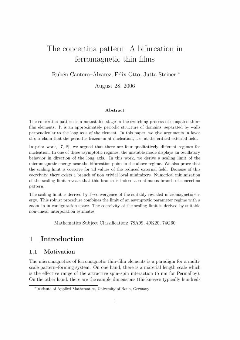


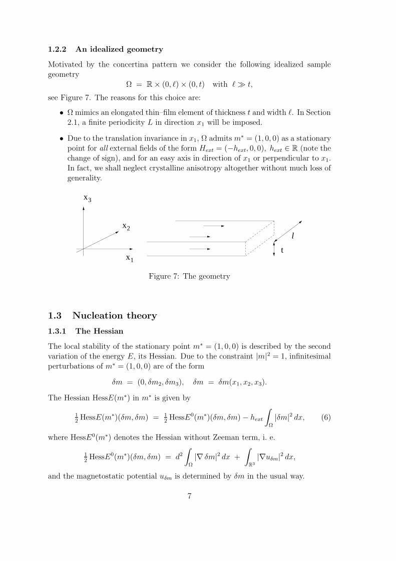

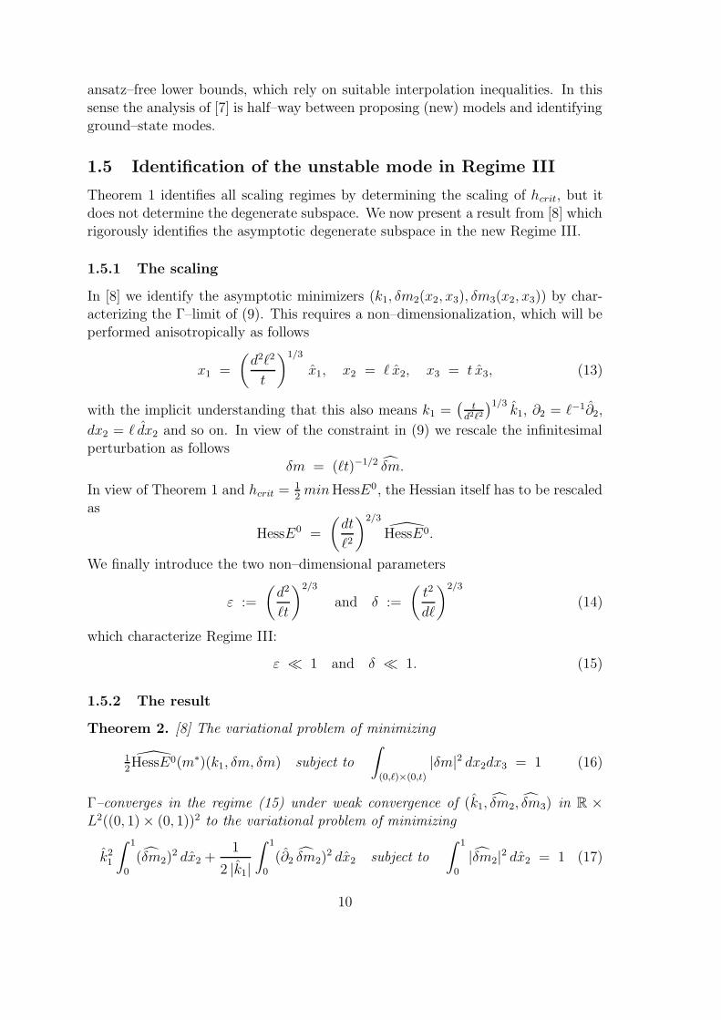
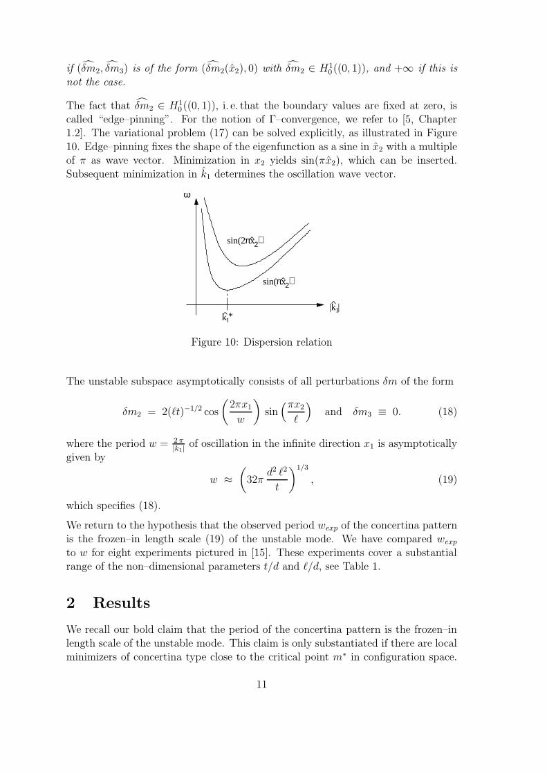


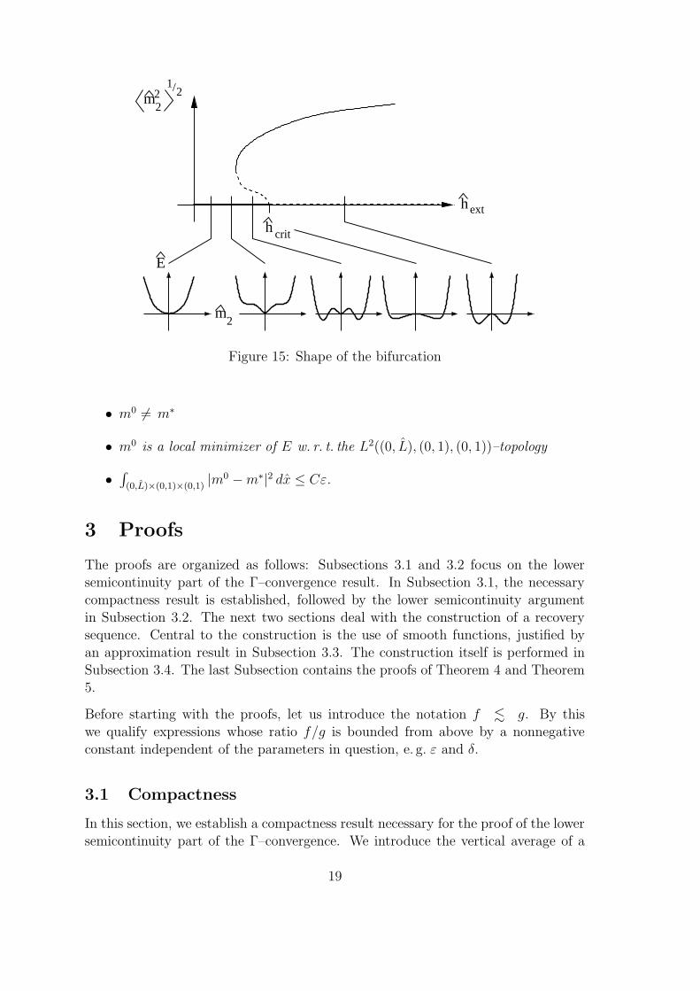
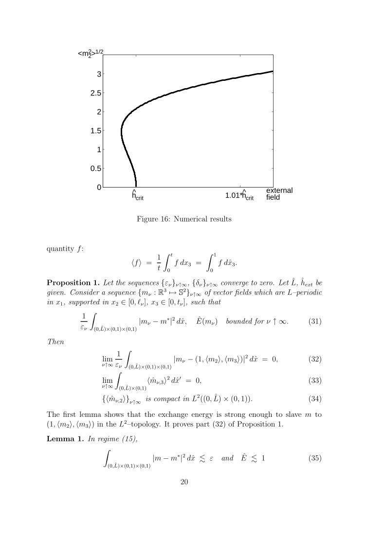


![· CONCERTINA JOURNAL, GERMAN CONCERTINA TUTOR, ETC. ... [large illustration of anglo concertina] ... Those with 30 to 40 keys have a Chromatic Scale of Semitones](https://static.documents.pub/doc/80x56/5b45f4a07f8b9af54b8b4af7/-concertina-journal-german-concertina-tutor-etc-large-illustration-of.jpg)


