THE CONFRONTATION BETWEEN GENERAL RELATIVITY AND

EXPERIMENT: A 1998 UPDATE

Clifford M. Will

McDonnell Center for the Space Sciences

Department of Physics

Washington University, St. Louis, MO 63130

ABSTRACT

The status of experimental tests of general relativity and of theoreti- cal frameworks for analyzing them is reviewed. Einstein’s equivalence principle (EEP) is well supported by experiments such as the E&v& experiment, tests of special relativity, and the gravitational redshift experiment. Future tests of EEP will search for new interactions aris- ing from unification or quantum gravity. Tests of general relativity have reached high precision, including the light deflection, the Shapiro time delay, the perihelion advance of Mercury, and the Nordtvedt ef- fect in lunar motion. Gravitational wave damping has been detected to half a percent using the binary pulsar, and new binary pulsar systems promise further improvements. When direct observation of gravita- tional radiation from astrophysical sources begins, new tests of general relativity will be possible.

*Support in part by NSF Grant 96-00049

@ 1998 by Clifford M. Will.

-15-

2 Tests of the Foundations of Gravitation

Theory

2.1 The Einstein Equivalence Principle

The principle of equivalence has historically played an important role in the devel-

opment of gravitation theory. Newton regarded this principle as such a cornerstone

of mechanics that he devoted the opening paragraph of the Principia to it. In

1907, Einstein used the principle as a basic element of general relativity. We now

regard the principle of equivalence as the foundation, not of Newtonian gravity or

of GR, but of the broader idea that spacetime is curved.

One elementary equivalence principle is the kind Newton had in mind when he

stated that the property of a body called “mass” is proportional to the “weight,”

and is known as the weak equivalence principle (WEP). An alternative statement

of WEP is that the trajectory of a freely falling body (one not acted upon by such

forces as electromagnetism and too small to be affected by tidal gravitational

forces) is independent of its internal structure and composition. In the simplest

case of dropping two different bodies in a gravitational field, WEP states that the

bodies fall with the same acceleration.

A more powerful and far-reaching equivalence principle is known as the Ein-

stein equivalence principle (EEP). It states that (i) WEP is valid, (ii) the out-

come of any local non-gravitational experiment is independent of the velocity of

the freely-falling reference frame in which it is performed, and (iii) the outcome

of any local non-gravitational experiment is independent of where and when in

the universe it is performed. The second piece of EEP is called local Lorentz

invariance (LLI), and the third piece is called local position invariance (LPI).

For example, a measurement of the electric force between two charged bodies

is a local non-gravitational experiment; a measurement of the gravitational force

between two bodies (Cavendish experiment) is not.

The Einstein equivalence principle is the heart and soul of gravitational theory,

for it is possible to argue convincingly that if EEP is valid, then gravitation must

be a “curved spacetime” phenomenon, in other words, the effects of gravity must

be equivalent to the effects of living in a curved spacetime. As a consequence of

this argument, the only theories of gravity that can embody EEP are those that

satisfy the postulates of “metric theories of gravity,” which are (i) spacetime is

endowed with a symmetric metric, (ii) the trajectories of freely falling bodies are

geodesics of that metric, and (iii) in local freely falling reference frames, the non-

gravitational laws of physics are those written in the language of special relativity.

The argument that leads to this conclusion simply notes that, if EEP is valid, then

in local freely falling frames, the laws governing experiments must be independent

of the velocity of the frame (local Lorentz invariance), with constant values for the

various atomic constants (in order to be independent of location). The only laws

we know of that fulfill this are those that are compatible with special relativity,

such as Maxwell’s equations of electromagnetism. Furthermore, in local freely

falling frames, test bodies appear to be unaccelerated; in other words they move

on straight lines, but such “locally straight” lines simply correspond to “geodesics”

in a curved spacetime (TEGP 2.3).

General relativity is a metric theory of gravity, but then so are many others,

including the Brans-Dicke theory. The nonsymmetric gravitation theory (NGT)

of Moffat is not a metric theory, neither is superstring theory (see Sec. 2.3). So the

notion of curved spacetime is a very general and fundamental one, and therefore

it is important to test the various aspects of the Einstein Equivalence Principle

thoroughly.

A direct test of WEP is the comparison of the acceleration of two laboratory-

sized bodies of different composition in an external gravitational field. If the

principle were violated, then the accelerations of different bodies would differ.

The simplest way to quantify such possible violations of WEP in a form suitable

for comparison with experiment is to suppose that for a body with inertial mass

mr, the passive gravitational mass mp is no longer equal to mr, so that in a

gravitational field g, the acceleration is given by mra = mpg. Now the inertial

mass of a typical laboratory body is made up of several types of mass-energy:

rest energy, electromagnetic energy, weak-interaction energy, and so on. If one of

these forms of energy contributes to mp differently than it does to rn1, a violation

of WEP would result. One could then write

mp = rnI •t c qAEAfc2, A

where EA is the internal energy of the body generated by interaction A, and nA

is a dimensionless parameter that measures the strength of the violation of WEP

induced by that interaction, and c is the speed of light. A measurement or limit on

the fractional difference in acceleration between two bodies then yields a quantity

-IT-

4

However, there is one class of experiments that can be interpreted as “clean,”

high-precision tests of local Lorentz invariance. These are the “mass anisotropy”

experiments: the classic versions are the Hughes-Drever experiments, performed

in the period 1959-60 independently by Hughes and collaborators at Yale Univer-

sity, and by Drever at Glasgow University [TEGP 2.4(b)]. Dramatically improved

versions were carried out during the late 1980s using laser-cooled trapped atom

techniques (TEGP 14.1). A simple and useful way of interpreting these experi-

ments is to suppose that the electromagnetic interactions suffer a slight violation

of Lorentz invariance, through a change in the speed of electromagnetic radiation

c relative to the limiting speed of material test particles (ce, chosen to be unity

via a choice of units), in other words, c # 1 (see Sec. 2.2.3). Such a violation

necessarily selects a preferred universal rest frame, presumably that of the cosmic

background radiation, through which we are moving at about 300 km/s. Such

a Lorentz-non-invariant electromagnetic interaction would cause shifts in the en-

ergy levels of atoms and nuclei that depend on the orientation of the quantization

axis of the state relative to our universal velocity vector, and on the quantum

numbers of the state. The presence or absence of such energy shifts can be ex-

amined by measuring the energy of one such state relative to another state that

is either unaffected or is affected differently by the supposed violation. One way

is to look for a shifting of the energy levels of states that are ordinarily equally

spaced, such as the four J=3/2 ground states of the 7Li nucleus in a magnetic

field (Drever experiment); another is to compare the levels of a complex nucleus

with the atomic hyperfine levels of a hydrogen maser clock. These experiments

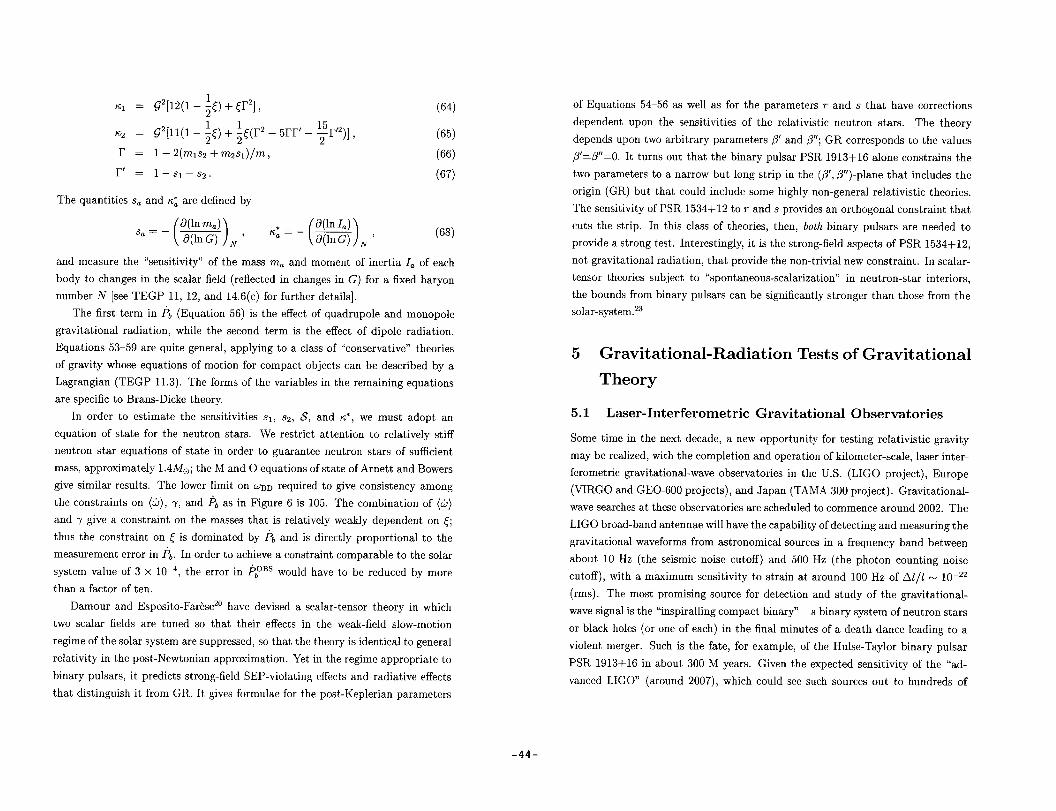
have all yielded extremely accurate results, quoted as limits on the parameter

6 = ce2 - 1 in Figure 2. Also included for comparison is the corresponding limit

obtained from Michelson-Morley type experiments.

Recent advances in atomic spectroscopy and atomic timekeeping have made it

possible to test LLI by checking the isotropy of the speed of light using one-way

propagation (as opposed to round-trip propagation, as in the Michelson-Morley

experiment). In one experiment, for example, the relative phases of two hydro-

gen maser clocks at two stations of NASA’s Deep Space Tracking Network were

compared over five rotations of the Earth by propagating a light signal one-way

along an ultrastable fiberoptic link connecting them (see Sec. 2.2.3). Although

the bounds from these experiments are not as tight as those from mass-anisotropy

experiments, they probe directly the fundamental postulates of special relativity,

TESTS OF LOCAL LORENTZ INVARIANCE

6

JPL

NIST

Harvard T

YEAR OF EXPERIMENT

Fig. 2. Selected tests of local Lorentz invariance showing bounds on parameter

6, which measures degree of violation of Lorentz invariance in electromagnetism.

Michelson-Morley, Joos, and Brillet-Hall experiments test isotropy of round-trip

speed of light, the latter experiment using laser technology. Centrifuge, two-

photon absorption (TPA), and JPL experiments test isotropy of light speed using

one-way propagation. Remaining four experiments test isotropy of nuclear energy

levels. Limits assume speed of Earth of 300 km/s relative to the mean rest frame

of the universe.

-19-

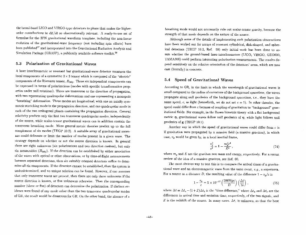
TESTS OF LOCAL POSITION INVARIANCE

Millisecond Pulsar

H-maser

Null Redshift

YEAR OF EXPERIMENT

1 Av/v = (l+a)AU/c* 1

Fig. 3. Selected tests of local position invariance via gravitational redshift experi-

ments, showing bounds on cy, which measures degree of deviation of redshift from

the formula Au/u = AU/c2.

Constant k

Fine structure constant

a = e2/hc

Limit on k/k

per Hubble time

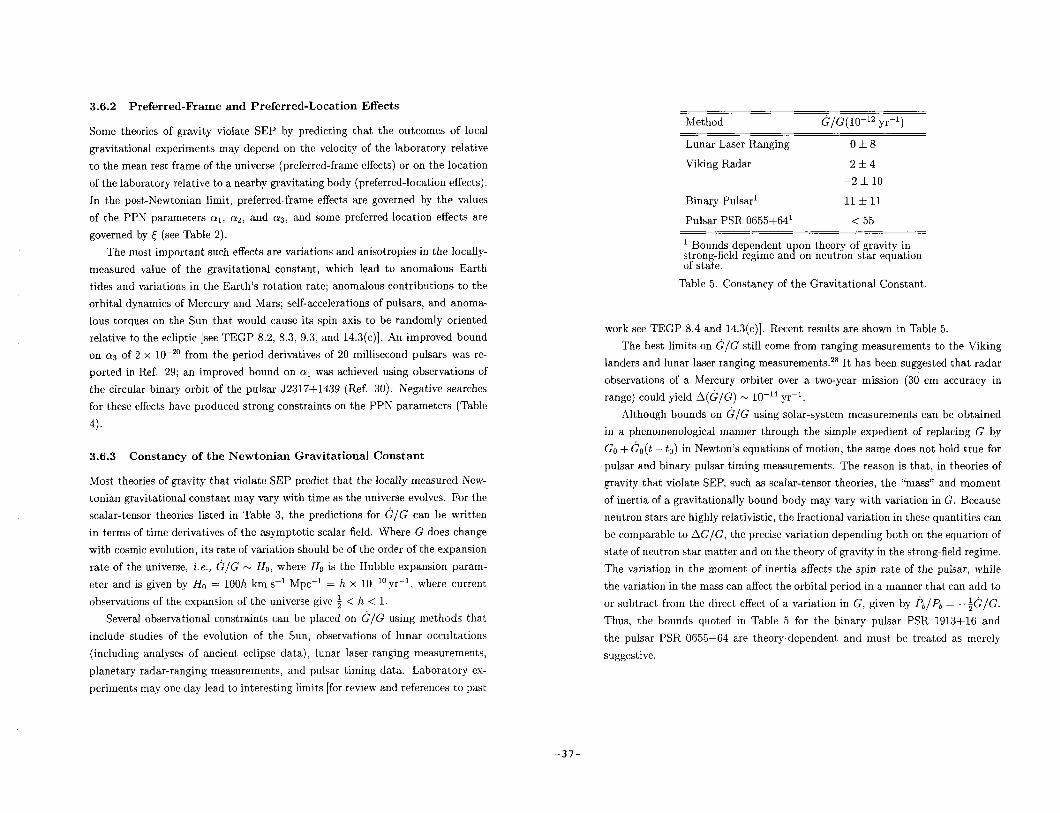
1.2 x 1O’O yr Method

4 x 10-4 H-maser vs Hg ion clock”

6 x 1O-7 Oklo Natural Reactor”

6 x 1O-5 21-cm vs molecular absorption

at 2 = 0.7 (Ref. 12)

Weak interaction constant 1

p = Gfmic/fi3 0.1

0.06

e-p mass ratio 1

ia7Re, 40K decay rates

Oklo Natural Reactor”

Big bang nucleosynthesisr3

Mass shift in quasar

spectra at 2 N 2

Proton g-factor (gs) 10-s 21-cm vs molecular absorption

at 2 = 0.7 (Ref. 12)

Table 1. Bounds on cosmological variation of fundamental constants of non-

gravitational physics. For references to earlier work, see TEGP 2.4(c).

general relativistic effects is a whopping 40 microseconds per day (60~s from the

gravitational redshift, and -20~s from time dilation). If these effects were not

accurately accounted for, GPS would fail to function at its stated accuracy. This

represents a welcome practical application of GR!

Local position invariance also refers to position in time. If LPI is satisfied, the

fundamental constants of non-gravitational physics should be constants in time.

Table 1 shows current bounds on cosmological variations in selected dimensionless

constants. For discussion and references to early work, see TEGP 2.4(c).

2.2 Theoretical Frameworks for Analyzing EEP

2.2.1 Schiff’s Conjecture

Because the three parts of the Einstein equivalence principle discussed above are

so very different in their empirical consequences, it is tempting to regard them

as independent theoretical principles. On the other hand, any complete and self-

-21-

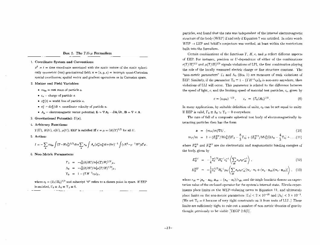
Box 1. The THtp Formalism

1. Coordinate System and Conventions:

z” = t = time coordinate associated with the static nature of the static spheri- cally symmetric (SSS) gravitational field; x = (2, y, z) = isotropic quasi-Cartesian spatial coordinates; spatial vector and gradient operations as in Cartesian space.

2. Matter and Field Variables:

l mea = rest mass of particle a.

. e, = charge of particle a.

l z!(t) = world line of particle a.

. ut = dxi/dt = coordinate velocity of particle a.

l A, = electromagnetic vector potential; E = VA0 - aA/&, B = V x A.

3. Gravitational Potential: U(x).

4. Arbitrary Functions:

T(U), H(U), e(U), p(U); EEP is satisfied iff E =/I = (H/Z’)‘/* for all U.

5. Action:

I= -Cmoa (1

/(T-Hv;)‘/*dt+~ e, /AJzDY)y:Ldt+(8z+ /(cE*-p-‘B2)d4z. D

6. Non-Metric Parameters:

ro = -c~(a/aU) ln[~(T/H)‘12]0,

A0 = -ci(a/tW) ln~(T/H)‘/*]e ,

To = 1 - (TH-‘Ep)o,

where CO = (Te/Hn)i/* and subscript “0” refers to a chosen point in space. If EEP is satisfied, PO E A0 = TO = 0.

particles, and found that the rate was independent of the internal electromagnetic

structure of the body (WEP) if and only if Equation 7 was satisfied. In other words

WEP + EEP and Schiff’s conjecture was verified, at least within the restrictions

built into the formalism.

Certain combinations of the functions T, H, E, and p reflect different aspects

of EEP. For instance, position or U-dependence of either of the combinations

c(T/H)l/’ and p(T/H)112 signals violations of LPI, the first combination playing

the role of the locally measured electric charge or fine structure constant. The

“non-metric parameters” IO and A0 (Box 1) are measures of such violations of

EEP. Similarly, if the parameter TO = 1 - (TH-‘E~)~ is non-zero anywhere, then

violations of LLI will occur. This parameter is related to the difference between

the speed of light, c, and the limiting speed of material test particles, c,, given by

c = (EO~O)-‘I* , c, = (To/Ho)1/2. (91

In many applications, by suitable definition of units, cc can be set equal to unity.

If EEP is valid, Fe z A0 E To = 0 everywhere.

The rate of fail of a composite spherical test body of electromagnetically in-

teracting particles then has the form

a = (mp/m)VU, (10)

mp/m = 1 + (EB”s/Mc;)[2ro - fg,] + (EB”s/Mc;)[2Ao - $r,] +. ,(ll)

where Eis and EfS are the electrostatic and magnetostatic binding energies of

the body, given by

(12) EES I3 =

EMS B = eaebr,-d[va vb + (Va nab)(Vb . nab)1 , (I31

where T,b = Jx, -&I, nab = (X=-X*)/ r& and the angle brackets denote an expec-

tation value of the enclosed operator for the system’s internal state. E&v& exper-

iments place limits on the WEP-violating terms in Equation 11, and ultimately

place limits on the non-metric parameters ]lYc] < 2 x 10-i’ and ]Ao] < 3 x 10-6.

(We set TO = 0 because of very tight constraints on it from tests of LLI .) These

limits are sufficiently tight to rule out a number of non-metric theories of gravity

thought previously to be viable [TEGP 2.6(f)].

-23-

where 4 = 27rvL, v is the maser frequency, L = 21 km is the baseline, and where

n and no are unit vectors along the direction of propagation of the light, at a given

time, and at the initial time of the experiment, respectively. The observed limit on

a diurnal variation in the relative phase resulted in the bound lc-’ - 11 < 3 x 10m4.

Tighter bounds were obtained from a “two-photon absorption” (TPA) experiment,

and a 1960s series of “Mossbauer-rotor” experiments, which tested the isotropy of

time dilation between a gamma ray emitter on the rim of a rotating disk and an

absorber placed at the center.14

2.3 EEP, Particle Physics, and the Search for New Inter-

actions

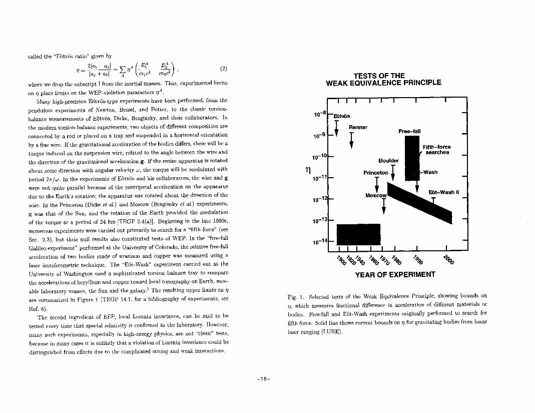
In 1986, as a result of a detailed reanalysis of Eotvijs’ original data, Fischbach

et al. suggested the existence of a fifth force of nature, with a strength of about a

percent that of gravity, but with a range (as defined by the range X of a Yukawa

potential, e- ‘1’ r of a few hundred meters. This proposal dovetailed with earlier / )

hints of a deviation from the inverse-square law of Newtonian gravitation derived

from measurements of the gravity profile down deep mines in Australia, and with

ideas from particle physics suggesting the possible presence of very low-mass par-

ticles with gravitational-strength couplings. During the next four years numerous

experiments looked for evidence of the fifth force by searching for composition-

dependent differences in acceleration, with variants of the Eiitviis experiment or

with free-fall Galileo-type experiments. Although two early experiments reported

positive evidence, the others all yielded null results. Over the range between one

and lo4 meters, the null experiments produced upper limits on the strength of

a postulated fifth force between 10m3 and lo@ of the strength of gravity. Inter-

preted as tests of WEP (corresponding to the limit of infinite-range forces), the

results of the free-fall Galileo experiment, and of the E&-Wash III experiment are

shown in Figure 1. At the same time, tests of the inverse-square law of gravity

were carried out by comparing variations in gravity measurements up tall towers

or down mines or boreholes with gravity variations predicted using the inverse

square law together with Earth models and surface gravity data mathematically

“continued” up the tower or down the hole. Despite early reports of anomalies,

independent tower, borehole, and seawater measurements now show no evidence

of a deviation. The consensus at present is that there is no credible experimental

evidence for a fifth force of nature. For reviews and bibliographies, see Refs. 8,

15, 16, and 17.

Nevertheless, theoretical evidence continues to mount that EEP is like/y to be

violated at some level, whether by quantum gravity effects, by effects arising from

string theory, or by hitherto undetected interactions, albeit at levels below those

that motivated the fifth-force searches. Roughly speaking, in addition to the pure

Einsteinian gravitational interaction, which respects EEP, theories such as string

theory predict other interactions which do not. In string theory, for example, the

existence of such EEP-violating fields is assured, but the theory is not yet mature

enough to enable calculation of their strength (relative to gravity), or their range

(whether they are long range, like gravity, or short range, like the nuclear and

weak interactions, or too short-range to be detectable) (for further discussion see

Ref. 6).

In one simple example, one can write the Lagrangian for the low-energy limit

of string theory in the so-called “Einstein frame, ” in which the gravitational La-

grangian is purely general relativistic:

where jpy is the non-physical metric, 8,” is the Ricci tensor derived from it, ‘p is a dilaton field, and G, U, and A? are functions of cp. The Lagrangian includes

that for the electromagnetic field F,,, and that for particles, written in terms of

Dirac spinors 4. This is not a metric representation because of the coupling of

cp to matter via i”vi(cp) and U(v). A conformal transformation fipV = F(p)g,,y,

T+? = F(p)-“I”$, puts the Lagrangian in the form (“Jordan” frame)

C = dT(s”“[~Wev - ~F(+$(P)WLP + &WW]

-U((p)g’vg~~Fp,Fvp + $[ie:ra(& + Qp + gA,) - ti(q)F’+) (21)

One may choose F(p) = const/Q((p)* so that the particle Lagrangian takes the

metric form (no coupling to cp), but the electromagnetic Lagrangian will still

couple non-metrically to U(v). The gravitational Lagrangian here takes the form

of a scalar-tensor theory (Sec. 3.3.2). But the non-metric electromagnetic term

will, in general, produce violations of EEP.

-25-

%

P c z Y

“absolute elements,” fields or equations whose structure and evolution are given

a priori, and are independent of the structure and evolution of the other fields of

the theory. These “absolute elements” typically include flat background metrics

17, cosmic time coordinates t, algebraic relationships among otherwise dynamical

fields, such as glly = ,,” h + k,k,, where h,, and k, may be dynamical fields.

General relativity is a purely dynamical theory since it contains only one grav-

itational field, the metric itself, and its structure and evolution are governed by

partial differential equations (Einstein’s equations). Brans-Dicke theory and its

generalizations are purely dynamical theories; the field equation for the metric

involves the scalar field (as well as the matter as source), and that for the scalar

field involves the metric. Rosen’s bimetric theory is a prior-geometric theory: it

has a non-dynamical, Riemann-flat background metric, v, and the field equations

for the physical metric g involve 17.

By discussing metric theories of gravity from this broad point of view, it is

possible to draw some general conclusions about the nature of gravity in differ-

ent metric theories, conclusions that are reminiscent of the Einstein equivalence

principle, but that are subsumed under the name “strong equivalence principle.”

Consider a local, freely falling frame in any metric theory of gravity. Let this

frame be small enough that inhomogeneities in the external gravitational fields

can be neglected throughout its volume. On the other hand, let the frame be large

enough to encompass a system of gravitating matter and its associated gravita-

tional fields. The system could be a star, a black hole, the solar system or a

Cavendish experiment. Call this frame a “quasi-local Lorentz frame.” To deter-

mine the behavior of the system we must calculate the metric. The computation

proceeds in two stages. First we determine the external behavior of the metric and

gravitational fields, thereby establishing boundary values for the fields generated

by the local system, at a boundary of the quasi-local frame LLfar” from the local

system. Second, we solve for the fields generated by the local system. But because

the metric is coupled directly or indirectly to the other fields of the theory, its

structure and evolution will be influenced by those fields, and in particular by the

boundary values taken on by those fields far from the local system. This will be

true even if we work in a coordinate system in which the asymptotic form of glly

in the boundary region between the local system and the external world is that

of the Minkowski metric. Thus the gravitational environment in which the local

gravitating system resides can influence the metric generated by the local system

via the boundary values of the auxiliary fields. Consequently, the results of local

gravitational experiments may depend on the location and velocity of the frame

relative to the external environment. Of course, local nonigravitational experi-

ments are unaffected since the gravitational fields they generate are assumed to

be negligible, and since those experiments couple only to the metric, whose form

can always be made locally Minkowskian at a given spacetime event. Local grav-

itational experiments might include Cavendish experiments, measurement of the

acceleration of massive self-gravitating bodies, studies of the structure of stars and

planets, or analyses of the periods of “gravitational clocks.” We can now make

several statements about different kinds of metric theories.

(i) A theory which contains only the metric g yields local gravitational physics

which is independent of the location and velocity of the local system. This follows

from the fact that the only field coupling the local system to the environment

is g, and it is always possible to find a coordinate system in which g takes the

Minkowski form at the boundary between the local system and the external envi-

ronment. Thus the asymptotic values of glLy are constants independent of location,

and are asymptotically Lorentz invariant, thus independent of velocity. General

relativity is an example of such a theory.

(ii) A theory which contains the metric g and dynamical scalar fields VA yields

local gravitational physics which may depend on the location of the frame but

which is independent of the velocity of the frame. This follows from the asymptotic

Lorentz invariance of the Minkowski metric and of the scalar fields, but now the

asymptotic values of the scalar fields may depend on the location of the frame.

An example is Brans-Dicke theory, where the asymptotic scalar field determines

the effective value of the gravitational constant, which can thus vary as ‘p varies.

(iii) A theory which contains the metric g and additional dynamical vector or

tensor fields or prior-geometric fields yields local gravitational physics which may

have both location and velocity-dependent effects.

These ideas can be summarized in the strong equivalence principle (SEP),

which states that (i) WEP is valid for self-gravitating bodies as well as for test

bodies, (ii) the outcome of any local test experiment is independent of the velocity

of the (freely falling) apparatus, and (iii) the outcome of any local test experiment

is independent of where and when in the universe it is performed. The distinction

between SEP and EEP is the inclusion of bodies with self-gravitational interac-

tions (planets, stars) and of experiments involving gravitational forces (Cavendish

-27-

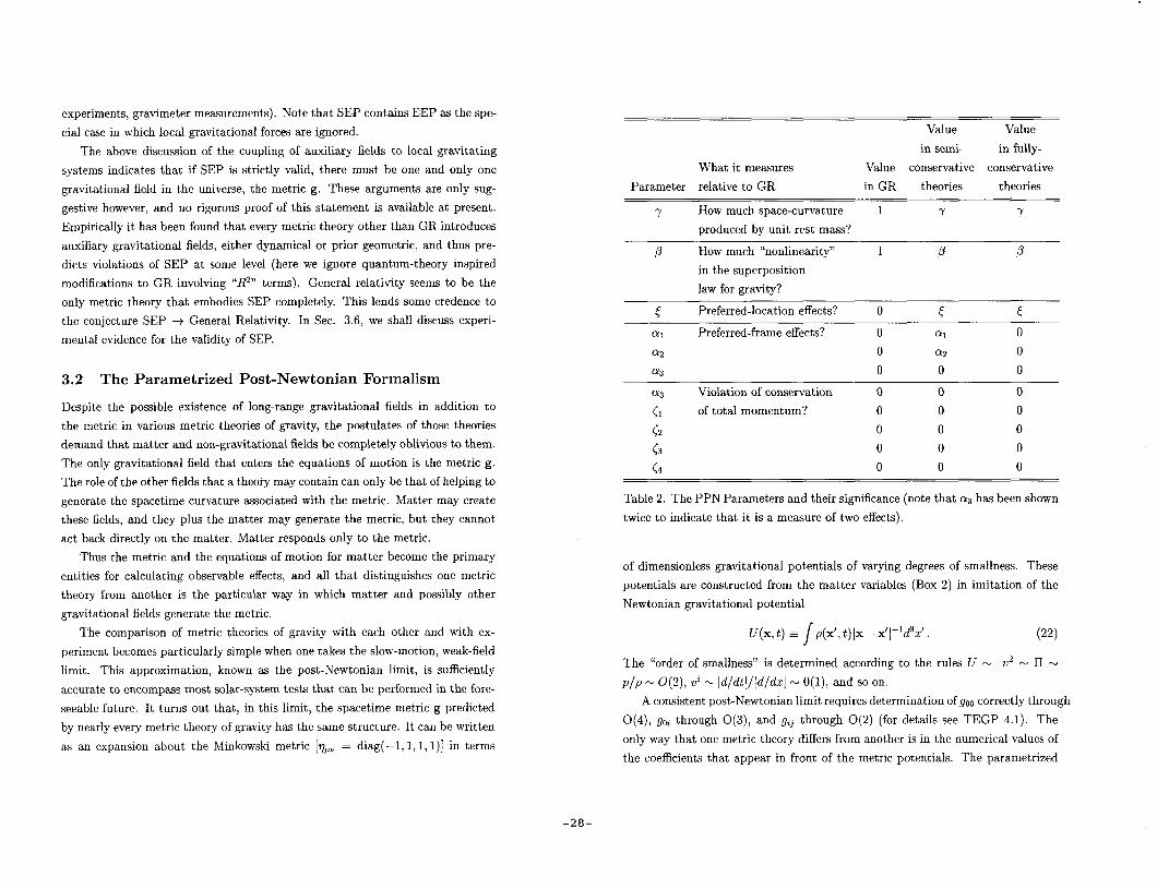
post-Newtonian (PPN ) formalism inserts parameters in place of these coefficients,

parameters whose values depend on the theory under study. In the current version

of the PPN formalism, summarized in Box 2, ten parameters are used, chosen in

such a manner that they measure or indicate general properties of metric theories

of gravity (Table 2). The parameters y and p are the usual Eddington-Robertson-

Schiff parameters used to describe the “classical” tests of GR; < is non-zero in any

theory of gravity that predicts preferred-location effects such as a galaxy-induced

anisotropy in the local gravitational constant GL (also called “Whitehead” ef-

fects); ai, (~2, crs measure whether or not the theory predicts post-Newtonian

preferred-frame effects; os, <I, <z, [s, <4 measure whether or not the theory pre-

dicts violations of global conservation laws for total momentum. In Table 2 we

show the values these parameters take (i) in GR, (ii) in any theory of gravity that

possesses conservation laws for total momentum, called “semi-conservative” (any

theory that is based on an invariant action principle is semi-conservative), and

(iii) in any theory that in addition possesses six global conservation laws for an-

gular momentum, called “fully conservative” (such theories automatically predict

no post-Newtonian preferred-frame effects). Semi-conservative theories have five

free PPN parameters (y, /3, <, cq, 02) while fully conservative theories have three

(7, B > 0 The PPN formalism was pioneered by Kenneth Nordtvedt, who studied the

post-Newtonian metric of a system of gravitating point masses, extending earlier

work by Eddington, Robertson, and Schiff (TEGP 4.2). A general and unified ver-

sion of the PPN formalism was developed by Will and Nordtvedt. The canonical

version, with conventions altered to be more in accord with standard textbooks

such as MTW, is discussed in detail in TEGP, Chapter 4. Other versions of the PPN

formalism have been developed to deal with point masses with charge, fluid with

anisotropic stresses, bodies with strong internal gravity, and post-post-Newtonian

effects (TEGP 4.2, 14.2).

3.3 Competing Theories of Gravity

One of the important applications of the PPN formalism is the comparison and

classification of alternative metric theories of gravity. The population of viable

theories has fluctuated over the years as new effects and tests have been discovered,

largely through the use of the PPN framework, which eliminated many theories

Box 2. The Parametrized Post-Newtonian Formalism

1. Coordinate System: The framework uses a nearly globally Lorentz coordinate system in which the coordinates are (t, xi, x2, x3). Three-dimensional, Euclidean vector notation is used throughout. All coordinate arbitrariness (“gauge freedom”) has been removed by specialization of the coordinates to the standard PPN gauge (TEGP 4.2). Units are chosen so that G = c = 1, where G is the physically measured Newtonian constant far from the solar system.

2. Matter Variables:

. p = density of rest mass as measured in a local freely falling frame momentarily comoving with the gravitating matter.

. vi = (&?/dt) = coordinate velocity of the matter.

. uli = coordinate velocity of PPN coordinate system relative to the mean rest- frame of the universe.

l p = pressure as measured in a local freely falling frame momentarily comoving with the matter.

. II = internal energy per unit rest mass. It includes all forms of non-rest-mass, non-gravitational energy, e.g., energy of compression and thermal energy.

3. PPN Parameters:

4. Metric:

900 = -I+ 2U - 2PU* - 2[@w + (27 + 2 + a3 + cl - 2.9a1

+2(3~ - 2P + 1+ CZ + 05.2 + 2(1+ c3p3 + 2(37 + 3~~ - 2[)@4

-(G - %)A - (a1 -a* - a3)w2U - cu2WidU,~ + (203 - al)t&

SOi = -i(4Y + 3 + a- a2 + G - 2F)lr - i(l +o* - <i + 2<)W,

-;(a1 - 2cq)W”U - a2ww,j

gi3 = (1 + ZyU)b,,

-29-

-OE-

Xloaq$ Bu!lls se yans ‘sauraqze uo!$ezy!un u! pue Smpl!nq [apour 1e3@010w -so3 u! mlndod LlaA atuoaaq hIlua3al amq 83 30 suoymy!poru Josual-mlsag .

koayl 3!I)auuq s,uasox s! a[dmsxa uv ‘(z’g’& ‘aas aas) suoymziasqo Lq pauym$suo3 dl@y uaaq amq $eq!f ‘slDa#a ,,aumq-pa~~a3a~d,, $%pald sa!loaq$ asaql 30 ISOW ‘+)am Iv@qd aql 0% uo!$~ppe u! ayam punol8ymq qeg e se yms sluaurala alrqosqs ql!M ‘S+IOaq~ ,+)auroaho!~d,, 30 ss’e~a aql o’$u! 11~3 sa!.Ioaql 30 laqumu v l

‘&I!~[aH pus ‘~paA~pSoN ‘~I!M bq pa!pn)s sa!loaql losua’$-cIo$>aa aql aw saldwvxx w+Qd alzymd JO dloaq’$ pIay 30 ‘ks ‘M~!A 30 lu!od aql uroq sa!Ioaql pa$‘~~gour -IlaM se pap&al aq pIno:, asaql30 Mad .sa!lladold .relm!lmd a$wlsnIp 01 JO qs!xa sa!loaql qms leqq aAold 0% paqUaAU! ‘sa!zoaql ,,uwu-MEI~S,, se pama!a aq p1no2 ~0861 pm S()L~I aql %pnp padolaaap sa!“oaql zyau~ aAyeura$[t? iluvfl l

‘9 m$deqD ‘d33J, u! ua~@ s! sa!loayl a.kyeuJa$[v 30 urmpuaduroa [[u3 v .

:pIo3-pz”aAas a.rz suosval aq& .aldumxa c+se[~ aql s! (q~oqs ~03 ‘aya-sue@ dIOaq$ ay3!a-SUsla-Zla!~-U~p~Or aq$ q3;qM 30 ‘$1 30 SUO!?)VXJ~pOUJ lOSUX,-IVlV3S 30 weI3 pzaua8 aql puv h~!nyqaI IwauaB uo smo3 ~pzeqs ahi ‘sam$aaI asaql UI

.pa$uam! uaaq amq sa!loaql alqyA blp!lualod ‘Man SB pa~en$m~ osl’e ‘se9 uoye[ndod dIoaq$ aq~ ‘a[qe!A aq 0% b[sno!AaId r@noq$

‘((lLZ-~)c!gd+(d/d+nZ+,n+LI+T).~?nd = C?J

(d/d + nz + zn + II f r)@ = ,,,L

(nz+ p+LI+ IId = OOJ

‘/‘EP!(,x - x;~x--~:) ,a],d J = ?M ‘,xspIJx-xI

;n,d / z.r “/i

,xsp//x - XI ,d I

= P@ ‘,xspIIx-~I ,ILd /

&@ ‘,xspI~y--xI In/ d /

= Z@

/ = ‘I$ ’ “Epz[(,:‘lY,) X]+j s =Y

,,XEP,“SP lrrx-FI l,,x--xl FI - Ix xl - - - . IF - x ,,x - ,x > Lx - x),P,d J = M@

lxSP ((,x $ixx! x),,j J = ‘% ‘ ,ZEP IF - XI

,d J = R

(panu!~uo3) ‘Z X08

Arbitrary Cosmic PPN Parameters

Functions Matching

Theory or Constants Parameters y P t ffl a2

General Relativity none none 1 1 00 0

Scalar-Tensor

Brans-Dicke W 40 (l+w) P+w) 1 00 0

General A(v), V(v) PO B 1+h 0 0 0 Rosen’s Bimetric none co, Cl 1 1 0 0 a-1

Cl

Table 3. Metric Theories and Their PPN Parameter Values (cya = <% = 0 for all

cases)

61= 0, where

1 = (167w’ / R(-g)‘/2d4x + Im(&,gpv) ,

where R is the Ricci scalar, and 1, is the matter action, which depends on matter

fields $J, universally coupled to the metric g. By varying the action with respect

to Qpv, we obtain the field equations

G,, = R,, - ;g,,R = %rGT,, , (24)

where Tpy is the matter energy-momentum tensor. General covariance of the

matter action implies the equations of motion TPYiy = 0; varying I,,, with respect

to $M yields the matter field equations. By virtue of the absence of prior-geometric

elements, the equations of motion are also a consequence of the field equations

via the Bianchi identities Gp”;” = 0.

The general procedure for deriving the post-Newtonian limit is spelled out in

TEGP 5.1, and is described in detail for GR in TEGP 5.2. The PPN parameter

values are listed in Table 3.

3.3.2 Scalar-Tensor Theories

These theories contain the metric g, a scalar field cp, a potential function V(q),

and a coupling function A(p) (generalizations to more than one scalar field have

also been carried out”). For some purposes, the action is conveniently written in

a non-metric representation, sometimes denoted the “Einstein frame,” in which

the gravitational action looks exactly like that of GR:

i = (lGaG)-‘/[A - 2~r”“&,498,,cp - V((p)](-ij)“*d4z + I,(&, A*((p)j,,), (25)

where l? = GUI? TV is the Ricci scalar of the “Einstein” metric iflU. [Apart from

the scalar potential term V(p), th’ is corresponds to Equation (20) with e(cp) z

(47&-i, U(p) = 1, and &‘(cp) K A(p).] This representation is a “non-metric”

one because the matter fields &, couple to a combination of cp and &“. Despite

appearances, however, it is a metric theory, because it can be put into a metric

representation by identifying the “physical metric”

gpv = A’((P)& (26)

The action can then be rewritten in the metric form

I= (16rG)-’ /[bhR - ~-‘w(~)g’““~,d&~ - 42V](-g)1’2d4x + Im($m,gpv) , (27)

where

4 = A(P)-~,

3+2w(4+) = a(p)-“,

4~) z 4ln A(cp))lG. (28)

The Einstein frame is useful for discussing general characteristics of such theories,

and for some cosmological applications, while the metric representation is most

useful for calculating observable effects. The field equations, post-Newtonian limit

and PPN parameters are discussed in TEGP 5.3, and the values of the PPN

parameters are listed in Table 3.

The parameters that enter the post-Newtonian limit are

w = w(do), A = [(dw/d4)(3 + 2~)~*(4 + 2w)-‘I$, , (29)

where @a is the value of 4 today far from the system being studied, as determined

by appropriate cosmological boundary conditions. The following formula is also

useful: l/(2 + w) = 2&(1 + ai). In Brans-Dicke theory [w(4) = constant],

the larger the value of w, the smaller the effects of the scalar field, and in the

-3l-

Fig. 4. Geometry of light deflection measurements.

second “y/2” varies from theory to theory. Thus, calculations that purport to

derive the full deflection using the equivalence principle alone are incorrect.

The prediction of the full bending of light by the Sun was one of the great

successes of Einstein’s GR. Eddington’s confirmation of the bending of optical

starlight observed during a solar eclipse in the first days following World War I

helped make Einstein famous. However, the experiments of Eddington and his

co-workers had only 30 percent accuracy, and succeeding experiments were not

much better: the results were scattered between one half and twice the Einstein

value (Figure 5), and the accuracies were low.

However, the development of very-long-baseline radio interferometry (VLBI)

produced greatly improved determinations of the deflection of light. These tech-

niques now have the capability of measuring angular separations and changes in

angles as small as 100 microarcseconds. Early measurements took advantage of

a series of heavenly coincidences: each year, groups of strong quasistellar radio

sources pass very close to the Sun (as seen from the Earth), including the group

3C273, 3C279, and 3C48, and the group 0111+02, 0119+11, and 0116f08. As

the Earth moves in its orbit, changing the lines of sight of the quasars relative to

the Sun, the angular separation 68 between pairs of quasars varies (Equation 32).

The time variation in the quantities d, d,, x, and @r in Equation 32 is determined

using an accurate ephemeris for the Earth and initial directions for the quasars,

and the resulting prediction for 66’ as a function of time is used as a basis for

a least-squares fit of the measured 68, with one of the fitted parameters being

the coefficient f(1 + y). A number of measurements of this kind over the period

1 .oo

0.95

THE PARAMETER (l+y)/2

!I + P + ’ I I I

1-1 VLBI

0 0 f 0

Hipparcos

P PSR 1937+21

4 - 1 _ Viking

1940 1960 1970 1980 1990

YEAR OF EXPERIMENT 2000

Fig. 5. Measurements of the coefficient (1 +y)/2 from light deflection and time de-

lay measurements. General relativity value is unity. Arrows denote anomalously

large values from 1929 and 1936 eclipse expeditions. Shapiro time-delay measure-

ments using Viking spacecraft and VLBI light deflection measurements yielded

agreement with GR to 0.1 percent. Hipparcos denotes the optical astrometry

satellite.

-33-

Parameter Effect Limit Remarks

Y-l

P-1

E Ql

Q2

ff3

7/l G G

c3

c4

time delay

light deflection

perihelion shift

Nordtvedt effect

Earth tides

orbital polarization

spin precession

pulsar acceleration

Nordtvedt effect

binary acceleration

Newton’s 3rd law -

2 x 10-s

3 x 10-4

3 x 10-a

6 x 1O-4 10-S

4 x 10-4 2 x 10-4 4 x 10-7 2 x 10-20

10-3 2 x 10-2 4 x 10-5

10-S

Viking ranging

VLBI

J2 = 10m7 from helioseismology

n=4@-y-3assumed

gravimeter data

Lunar laser ranging

PSR J2317+1439

solar alignment with ecliptic

pulsar P statistics

lunar laser ranging

combined PPN bounds

pp for PSR 1913+16

Lunar acceleration

not independent

‘Here n = 4p - 7 - 3 - 10</3 - ai - 2ff2/3 - 2ci13 - Czl3.

Table 4. Current Limits on the PPN Parameters.

The predicted advance, A5 , per orbit, including both relativistic PPN contri-

butions and the Newtonian contribution resulting from a possible solar quadrupole

moment, is given by

A3 = (6nm/p)[;(2+2y-b)+; (~LY~--cYz+(Y~+~CZ)~/~+J~(R~/~~~)], (35)

where m = mr + mz and /I = mi m2/m are the total mass and reduced mass of the

two-body system respectively; p = a(1 - e”) is the semi-latus rectum of the orbit,

with a the semi-major axis and e the eccentricity; R is the mean radius of the

oblate body; and Jz is a dimensionless measure of its quadrupole moment, given

by Jz = (C - A)/mlR2, where C and A are the moments of inertia about the

body’s rotation and equatorial axes, respectively (for details of the derivation see

TEGP 7.3). We have ignored preferred-frame and galaxy-induced contributions

to A3; these are discussed in TEGP 8.3.

The first term in Equation 35 is the classical relativistic perihelion shift, which

depends upon the PPN parameters y and /3. The second term depends upon

the ratio of the masses of the two bodies; it is zero in any fully conservative

theory of gravity (cyi = cys = cys = <z = 0); it is also negligible for Mercury, since

dm- I mMerc ma z 2 x 10m7. We shall drop this term henceforth. The third term

depends upon the solar quadrupole moment J2. For a Sun that rotates uniformly

with its observed surface angular velocity, so that the quadrupole moment is

produced by centrifugal flattening, one may estimate J2 to be N 1 x 10e7. This

actually agrees reasonably well with values inferred from rotating solar models

that are in accord with observations of the normal modes of solar oscillations

(helioseismology). Substituting standard orbital elements and physical constants

for Mercury and the Sun, we obtain the rate of perihelion shift &, in seconds of

arc per century,

ci = 42.“98 [;(2 + 27 - /3) + 3 x 10-4(J2/10-7)] (36)

Now, the measured perihelion shift of Mercury is known accurately: after the

perturbing effects of the other planets have been accounted for, the excess shift is

known to about 0.1 percent from radar observations of Mercury since 1966. The

solar oblateness effect is smaller than the observational error, so we obtain the

PPN bound (27 - /r’ - l( < 3 x 10p3.

-35-

4 II

3.6.2 Preferred-Frame and Preferred-Location Effects

Some theories of gravity violate SEP by predicting that the outcomes of local

gravitational experiments may depend on the velocity of the laboratory relative

to the mean rest frame of the universe (preferred-frame effects) or on the location

of the laboratory relative to a nearby gravitating body (preferred-location effects).

In the post-Newtonian limit, preferred-frame effects are governed by the values

of the PPN parameters ~1, CQ, and os, and some preferred-location effects are

governed by [ (see Table 2).

The most important such effects are variations and anisotropies in the locally-

measured value of the gravitational constant, which lead to anomalous Earth

tides and variations in the Earth’s rotation rate; anomalous contributions to the

orbital dynamics of Mercury and Mars; self-accelerations of pulsars, and anoma-

lous torques on the Sun that would cause its spin axis to be randomly oriented

relative to the ecliptic [see TEGP 8.2, 8.3, 9.3, and 14.3(c)]. An improved bound

on CQ of 2 x 10pzo from the period derivatives of 20 millisecond pulsars was re-

ported in Ref. 29; an improved bound on al was achieved using observations of

the circular binary orbit of the pulsar 52317+1439 (Ref. 30). Negative searches

for these effects have produced strong constraints on the PPN parameters (Table

4).

3.6.3 Constancy of the Newtonian Gravitational Constant

Most theories of gravity that violate SEP predict that the locally measured New-

tonian gravitational constant may vary with time as the universe evolves. For the

scalar-tensor theories listed in Table 3, the predictions for d/G can be written

in terms of time derivatives of the asymptotic scalar field. Where G does change

with cosmic evolution, its rate of variation should be of the order of the expansion

rate of the universe, i.e., G/G N Ho, where Ho is the Hubble expansion param-

eter and is given by Ho = 1OOh km s-i Mpc-’ = h x lO-l’yr-‘, where current

observations of the expansion of the universe give f < h < 1.

Several observational constraints can be placed on G/G using methods that

include studies of the evolution of the Sun, observations of lunar occultations

(including analyses of ancient eclipse data), lunar laser-ranging measurements,

planetary radar-ranging measurements, and pulsar timing data. Laboratory ex-

periments may one day lead to interesting limits [for review and references to past

Method G/G(10-12 yr-‘)

Lunar Laser Ranging Of8

Viking Radar 2f4

-2flO

Binary Pulsar’ 11 f 11

Pulsar PSR 0655+64l < 55

1 Bounds dependent u strong-field regime an cr

on theory of gravity in

of state. on neutron star equation

Table 5. Constancy of the Gravitational Constant.

work see TEGP 8.4 and 14.3(c)]. R ecent results are shown in Table 5.

The best limits on G/G still come from ranging measurements to the Viking

landers and lunar laser ranging measurements. 28 It has been suggested that radar

observations of a Mercury orbiter over a two-year mission (30 cm accuracy in

range) could yield A(G/G) N lo-l4 yr-‘.

Although bounds on G/G using solar-system measurements can be obtained

in a phenomenological manner through the simple expedient of replacing G by

Go + G:o(t - to) in Newton’s equations of motion, the same does not hold true for

pulsar and binary pulsar timing measurements. The reason is that, in theories of

gravity that violate SEP, such as scalar-tensor theories, the “mass” and moment

of inertia of a gravitationally bound body may vary with variation in G. Because

neutron stars are highly relativistic, the fractional variation in these quantities can

be comparable to AG/G, the precise variation depending both on the equation of

state of neutron star matter and on the theory of gravity in the strong-field regime.

The variation in the moment of inertia affects the spin rate of the pulsar, while

the variation in the mass can affect the orbital period in a manner that can add to

or subtract from the direct effect of a variation in G, given by @b/P, = -$‘:/G.

Thus, the bounds quoted in Table 5 for the binary pulsar PSR 1913+16 and

the pulsar PSR 0655+64 are theory-dependent and must be treated as merely

suggestive.

-37-

i?

c k Y

as a “gyroscope,” with its axis perpendicular to the orbital plane. The predicted

precession is about two arcseconds per century, an effect first calculated by de

Sitter. This effect has been measured to about 0.7 percent using lunar laser

ranging data.”

For a gyroscope orbiting the Earth, the precession is about eight arcseconds per

year. The Stanford Gyroscope Experiment has as one of its goals the measurement

of this effect to 5 x 10e5 (see below).

3.7.3 Search for Gravitomagnetism

According to GR, moving or rotating matter should produce a contribution to the

gravitational field that is the analogue of the magnetic field of a moving charge

or a magnetic dipole. Although gravitomagnetism plays a role in a variety of

measured relativistic effects, it has not been seen to date, isolated from other

post-Newtonian effects. The Relativity Gyroscope Experiment (Gravity Probe

B or GP-B) at Stanford University, in collaboration with NASA and Lockheed-

Martin Corporation, is in the advanced stage of developing a space mission to

detect this phenomenon directly. 33 A set of four superconducting-niobium-coated,

spherical quartz gyroscopes will be flown in a low polar Earth orbit, and the

precession of the gyroscopes relative to the distant stars will be measured. In

the PPN formalism, the predicted effect of gravitomagnetism is a precession (also

known as the Lense-Thirring effect, or the dragging of inertial frames), given by

dS/dr = C&T x S , &- = -i(l+y+ $)[J-3n(n.J)]/r3, (44)

where J is the angular momentum of the Earth, n is a unit radial vector, and

T is the distance from the center of the Earth (TEGP 9.1). For a polar orbit

at about 650 km altitude, this leads to a secular angular precession at a rate

i(1 + y + aor) x 10e3 arcsec/yr. The accuracy goal of the experiment is about

0.5 milliarcseconds per year. The science instrument package and the spacecraft

are in the final phases of construction, with launch scheduled for early 2000.

Another proposal to look for an effect of gravitomagnetism is to measure the

relative precession of the line of nodes of a pair of laser-ranged geodynamics satel-

lites (LAGEOS), ideally with supplementary inclination angles; the inclinations

must be supplementary in order to cancel the dominant nodal precession caused by

the Earth’s Newtonian gravitational multipole moments. Unfortunately, the two

existing LAGEOS satellites are not in appropriately inclined orbits, and no plans

exist at present to launch a third satellite in a supplementary orbit. Nevertheless,

by combing nodal precession data from LAGEOS I and II with perigee advance

data from the slightly eccentric orbit of LAGEOS II, Ciufolini et al. reported a

partial cancellation of multipole effects, and a resulting 20 percent confirmation

of GR.34

3.7.4 Improved PPN Parameter Values

A number of advanced space missions have been proposed in which spacecraft

orbiters or landers and improved tracking capabilities could lead to significant im-

provements in values of the PPN parameters, of JZ of the Sun, and of G/G. For

example, a Mercury orbiter, in a two-year experiment, with 3 cm range capability,

could yield improvements in the perihelion shift to a part in 104, in y to 4 x 10e5,

in e/G to lo-r4 yr-‘, and in 52 to a few parts in lo*. Proposals are being devel-

oped, primarily in Europe, for advanced space missions which will have tests of

PPN parameters as key components, including GAIA, a high-precision astromet-

ric telescope (successor to Hipparcos), which could measure light-deflection and y

to the 10m6 level, and a solar orbit relativity test, which could measure y to 10m7

from time delay and light deflection measurements.

3.7.5 Gravitational-Wave Astronomy

A significant part of the field of experimental gravitation is devoted to building

and designing sensitive devices to detect gravitational radiation and to use gravity

waves as a new astronomical tool. The centerpieces of this effort are the US

Laser Interferometric Gravitational-wave Observatory (LIGO) and the European

VIRGO projects, which are currently under construction. This important topic

has been reviewed thoroughly elsewhere,35 and in this volume.

4 Stellar System Tests of Gravitational Theory

4.1 Binary Pulsars and General Relativity

The majority of tests of gravitational theory described so far have involved solar-

system dynamics or laboratory experiments. Although the results confirm GR,

-39-

-OP-

.po!lad as[nd sl! UT IIsaqz@,, 30 aXIap!aa ou UMO~S seq IwInd aq& 2uoysas Bu!a~asqo uaarnqaq sq~uour x!s 0% dn 30 sde8 al!dsap ‘srlg~. 30 ho~nsze uv ~YJ!M aseqd IwInd aql30 ~EYZ.I$ daay 1123 slaalasqo aql yzq1 asuas aql u! ,,wal3,, s! uoy!s!nb38 olep aql ‘azounaqpnd ‘s~~a~aSu!~eydtuo3 JaqloIo~epy 111013 aaq ‘ueaI3 dlaas!uo!lourI~)!qloaylsnq~ .rwInd ppap e dIay!l ~sour s! cy c~sql 3saBBns sc+uaunGhv drSuo!lnIoAa :y3qdcuo3 SF uoydwo3 aqv lvq$ paaayaq LI[wauaB s! $! ‘uoyueduroa aq$u1013 lajsue.rl sswu 30

JO p~18!s~vs~nd aql30 asd!ya ~~30 aauap!aa ou SF alaqq asnwaq pw (ax1 z) asol3 OS s! l!qJo aql asnsaaa ‘(9 aIqv&) pau!e$qo uaaq aAvq urals.k aql103 slalaurenzd Iw!sbqd pue Ie$!qlo aywnze Qaurallxa ‘(sura)sbs hu!q c)!do%ol$zads UT pasn spoqlaru 93!y-IaIddoa aql30 uo!slai\ paleJr8a)u! UB 0% slunocus q~!q~) saslnd 30

saw!% ~A!IJE aql 30 sashyew palyap uro~ .uo!ueduroa uaasun pal se ue q’$!~ $!q.ro brwuq asol3 B u! SW 69 po!lad ~XI!~IOU 30 rw[nd v 30 sqsuo:, ura& aqL

LEG9E.~o~h~ pue aspq Lq sam$Dal az!ld IaqoN paqs!Iqnd aql aas ‘sn$sls lua.ws puv .kano3s!p aql30 sfiaptal .IOJ .uoyza~ uoywpw pi2ro!yz~!~w9 30 slaaga aql pue ‘s3!urw1Lp Ie)!qlo uo spIay IEUO~~~~A~L? Ivu.ralu! 3ys!AyzIal 8110.1~s 30 spa33a aql :d~oaq$puoyv$!~t?18 30 sl3adss Mau Bu!qold 30 Lvyq!ssod aql dn pauado as[nH puo ~oph?& dq gI+ET61 Bsd IwInd heu!q aq$30 dlaaoX!p ~~61 aqL ‘J!UU[ Uv!UOlMaN-$SOd ‘uo~~om-~01s ‘p[ay-yeaM aq$ 0% spuodsalloa uo!$lod s!y,~ .hloay$ 1? 30 ,,suo!yLpald 30 a-seds,, aql 30 uoyod paly!l 7! Quo +sa) Iraq+

time dilation as the pulsar moves in its elliptical orbit at varying distances from

the companion and with varying speeds; i‘b, the rate of change of orbital period,

caused predominantly by gravitational radiation damping; and r and s = sini,

respectively the “range” and “shape” of the Shapiro time delay caused by the

companion, where i is the angle of inclination of the orbit relative to the plane of

the sky.

In GR, these post-Keplerian parameters can be related to the masses of the

two bodies and to measured Keplerian parameters by the equations [TEGP 12.1,

14.6(a)]

(ti) = 3(2a/Pb)5/3m2/3(1 - e’)-’ , (45) I II e(PJ27r)‘13m2m-‘/3(1 + m2/m), (46)

i* = -(1927r/5)(2Tm/P*)“‘“(p/m) (1 + ge2 + gel) (1 - e2)m7/2, (47)

s = sini, (48)

r = m2, (49)

where ml and rn2 denote the pulsar and companion masses, respectively. The

formula for (&) ignores possible non-relativistic contributions to the periastron

shift, such as tidally or rotationally induced effects caused by the companion [for

discussion of these effects, see TEGP 12.1(c)]. The formula for pb represents the

effect of energy loss through the emission of gravitational radiation, and makes

use of the “quadrupole formula” of GR (for a survey of the quadrupole and other

approximations for gravitational radiation, see Ref. 38); it ignores other sources

of energy loss, such as tidal dissipation [TEGP 12.1(f)].

The timing model that contains these parameters was developed by Damour,

Deruelle, and Taylor, superseding earlier treatments by Haugan, Blandford, Teukol-

sky, and Epstein. The current values for Keplerian and post-Keplerian parameters

are shown in Table 6.

The most convenient way to display these results is to plot the constraints they

imply for the two masses ml and m2, via Equations 45 and 46. These are shown

in Figure 6. From (ti) and y’ we obtain the values ml = 1.4411 f 0.0007M0 and

m2 = 1.3873 i 0.0007M0. Equation 47 then predicts the value l$ = -2.40243 f

0.00005 x lo-‘*. In order to compare the predicted value for I$ with the observed

value, it is necessary to take into account the effect of a relative acceleration

between the binary pulsar system and the solar system caused by the differential

rotation of the galaxy. This effect was previously considered unimportant when

@b was known only to ten percent accuracy. Damour and Taylor carried out a

careful estimate of this effect using data on the location and proper motion of

the pulsar, combined with the best information available on galactic rotation, and

found ~GAL

b ru -(1.7 * 0.5) x 10-14. (50)

Subtracting this from the observed &, (Table 5) gives the residual

@OBS = b -(2.408 zt O.OIO[OBS] zt O.O05[GAL]) x IO-‘*, (51)

which agrees with the prediction, within the errors. In other words,

g = 1.0023 f O.O041[OBS] zt O.O021[GAL]. b

The parameters r and s are not separately measurable with interesting accuracy

for PSR 1913+16 because the orbit’s 47” inclination does not lead to a substantial

Shapiro delay. -

The consistency among the measurements is also displayed in Figure 6, in

which the regions allowed by the three most precise constraints have a single

common overlap. This consistency provides a test of the assumption that the

two bodies behave as “point” masses, without complicated tidal effects, obeying

the general relativistic equations of motion including gravitational radiation. It

is also a test of the strong equivalence principle, in that the highly relativistic

internal structure of the neutron star does not influence its orbital motion, as

predicted by GR. Recent observations 3g indicate variations in the pulse profile,

which suggests that the pulsar is undergoing geodetic precession (Sec. 3.7.2) in an

amount consistent with GR, assuming that the pulsar’s spin is suitably misaligned

with the orbital angular momentum.

4.2 A Population of Binary Pulsars?

Since 1990, several new massive binary pulsars similar to PSR 1913+16 were

discovered, leading to the possibility of new or improved tests of GR.

PSR 1534+12. This is a binary pulsar system in our galaxy. Its pulses

are significantly stronger and narrower than those of PSR 1913+16, so timing

measurements are more precise, reaching 3~s accuracy. Its parameters are listed

-41-

MAS

S O

F CO

MPA

NIO

N (s

olar

mas

ses)

. a

B k

k %

5

4.3 Binary Pulsars and Alternative Theories

Soon after the discovery of the binary pulsar, it was widely hailed as a new testing

ground for relativistic gravitational effects. As we have seen in the case of GR, in

most respects, the system has lived up to, indeed exceeded, the early expectations.

In another respect, however, the system has only partially lived up to its

promise, namely as a direct testing ground for alternative theories of gravity.

The origin of this promise was the discovery that alternative theories of gravity

generically predict the emission of dipole gravitational radiation from binary star

systems. This additional form of gravitational radiation damping could, at least

in principle, be significantly stronger than the usual quadrupole damping, because

it depends on fewer powers of the parameter v/c, where v is the orbital velocity

and c is the speed of light, and it depends on the gravitational binding energy

per unit mass of the bodies, which, for neutron stars, could be as large as 40 per

cent. As one fulfillment of this promise, Will and Eardley worked out in detail

the effects of dipole gravitational radiation in the bimetric theory of Rosen, and,

when the first observation of the decrease of the orbital period was announced in

1978, the Rosen theory suffered a terminal blow (TEGP 12.3). A wide class of

alternative theories also fail the binary pulsar test because of dipole gravitational

radiation.

On the other hand, the early observations already indicated that, in GR, the

masses of the two bodies were nearly equal, so that, in theories of gravity that are

in some sense “close” to GR, dipole gravitational radiation would not be a strong

effect, because of the apparent symmetry of the system (technically, the amount

of dipole radiation depends on the difference between the gravitational binding

energy per unit mass for the two bodies). The Rosen theory, and others like

it, are not “close” to general relativity, except in their predictions for the weak-

field, slow-motion regime of the solar system. When relativistic neutron stars are

present, theories like these can predict strong effects on the motion of the bodies

resulting from their internal highly relativistic gravitational structure (violations

of the Strong Equivalence Principle). As a consequence, the masses inferred from

observations such as the periastron shift may be significantly different from those

inferred using general relativity, and may be different from each other, leading

to strong dipole gravitational radiation damping. By contrast, the Brans-Dicke

theory, which was the basis for Eardley’s discovery of the dipole radiation phe-

nomenon, is “close” to GR, roughly speaking within l/~nn of the predictions of

the latter, for large values of the coupling constant WnD (henceforth this notation

for the coupling constant is adopted to avoid confusion with the periastron angle).

Thus, despite the presence of dipole gravitational radiation, the binary pulsar pro-

vides at present only a weak test of Brans-Dicke theory, not yet competitive with

solar-system tests.

4.4 Binary Pulsars and Scalar-Tensor Theories

Making the usual assumption that both members of the system are neutron stars,

and using the methods summarized in TEGP Chapters 10-12, one can obtain

formulas for the periastron shift, the gravitational redshift/second-order Doppler

shift parameter, and the rate of change of orbital period, analogous to Equations

45-47. These formulas depend on the masses of the two neutron stars, on their

self-gravitational binding energy, represented by “sensitivities” s and K* and on

the Brans-Dicke coupling constant ~no. First, there is a modification of Kepler’s

third law, given by

Pb/27r = (a3/Bm)‘/*. (53)

Then, the predictions for (ti), y’ and l$ are

(ti) = 3(27r/P~)5/3m2/3(1 - e2)-1Pg-4/3,

y’ = e(P&r)1’3m2m-1’3 G-1/3(~G + Gm2/m + K;$) ,

+b = -(192r/5)(2sm/P~)5’3(p/m)K4/3F(e)

-4~(2zm/Pb)(l.l/m)<S2G(e),

(54)

(55)

(56)

where, to first order in E = (2 + ~sn)-i, we have

F(e) = i(l - e2)-7/2[rCi(l + se2 + ae4) - K2(ae2 + ic4)],

G(e) = (1 - e2)-5/2(1 + fe2),

s = .!?I - s*,

E = 1 - ((Sl + s2 - 2SiSZ)) 2 1

P = G[l - -5 + -<(si + s* - 2SiSZ)] , 3 3

a; = 1 - b-2,

‘71 = (1 - 2s*)E,

(57)

(58)

(59)

(60)

(61) (62) (63)

-43-

cn

megaparsecs, it has been estimated that from 3 to 100 annual inspiral events could

be detectable. Other sources, such as supernova core collapse events, instabilities

in rapidly rotating nascent neutron stars, signals from non-axisymmetric pulsars,

and a stochastic background of waves, may be detectable (for reviews, see Ref. 35

and articles in this volume).

Detailed observation of gravitational waves from such sources may provide the

means to test general relativistic predictions for the polarization and speed of the

waves, and for gravitational radiation damping.

Several of these tests can be realized using gravitational-waves from inspiralling

compact binaries. The analysis of gravitational-wave data from such sources will

involve some form of matched filtering of the noisy detector output against an

ensemble of theoretical “template” waveforms which depend on the intrinsic pa-

rameters of the inspiralling binary, such as the component masses, spins, and so

on, and on its inspiral evolution. How accurate must a template be in order to

“match” the waveform from a given source (where by a match we mean maximiz-

ing the cross-correlation or the signal-to-noise ratio)? In the total accumulated

phase of the wave detected in the sensitive bandwidth, the template must match

the signal to a fraction of a cycle. For two inspiralling neutron stars, around

16,000 cycles should be detected; this implies a phasing accuracy of 10W5 or bet-

ter. Since v/c N l/10 during the late inspiral, this means that correction terms

in the phasing at the level of (V/C)” or higher are needed. More formal analyses

confirm this intuition.42

Because it is a slow-motion system (U/C N 10p3), the binary pulsar is sen-

sitive only to the lowest-order effects of gravitational radiation as predicted by

the quadrupole formula. Nevertheless, the first correction terms of order v/c

and (v/c)’ to the quadrupole formula were calculated as early as 1976 (TEGP

10.3). These are now conventionally called “post-Newtonian” (PN) corrections,

with each power of v/c corresponding to half a post-Newtonian order (1/2PN), in

analogy with post-Newtonian corrections to the Newtonian equations of motion.43

But for laser-interferometric observations of gravitational waves, the bottom

line is that, in order to measure the astrophysical parameters of the source and to

test the properties of the gravitational waves, it is necessary to derive the gravita-

tional waveform and the resulting radiation back-reaction on the orbit phasing at

least to 2PN, or second post-Newtonian order, O[(V/C)~], beyond the quadrupole

approximation, and probably to 3PN order.

5.2 Post-Newtonian Generation of Gravitational Waves

The generation of gravitational radiation is a long-standing problem that dates

back to the first years following the publication of GR, when Einstein calcu-

lated the gravitational radiation emitted by a laboratory-scale object using the

linearized version of GR. Shortly after the discovery of the binary pulsar PSR

1913+16 in 1974, questions were raised about the foundations of the “quadrupole

formula” for gravitational radiation damping (and in some quarters, even about

its quantitative validity). These questions were answered in part by theoretical

work designed to shore up the foundations of the quadrupole approximation,44

and in part (perhaps mostly) by the agreement between the predictions of the

quadrupole formula and the observed rate of damping of the pulsar’s orbit. In

1976, the post-Newtonian corrections to the quadrupole formula were of purely

academic, rather than observational, interest.

The challenge of providing accurate templates for LIGO-VIRGO data analysis

has led to major efforts to calculate gravitational waves to high PN order. Three

approaches have been developed.

The BDI approach of Blanchet, Damour, and Iyer is based on a mixed post-

Newtonian and “post-Minkowskian” framework for solving Einstein’s equations

approximately, developed in a long series of papers by Damour and colleagues.45

The idea is to solve the vacuum Einstein equations in the exterior of the material

sources extending out to the radiation zone in an expansion (“post-Minkowskian”)

in “nonlinearity” (effectively an expansion in powers of Newton’s constant G), and

to express the asymptotic solutions in terms of a set of formal, time-dependent,

symmetric and trace-free (STF) multipole moments.46 Then, in a near zone within

one characteristic wavelength of the radiation, the equations including the mate-

rial source are solved in a slow-motion approximation (expansion in powers of l/c)

that yields a set of STF source multipole moments expressed as integrals over the

“effective” source, including both matter and gravitational field contributions.

The solutions involving the two sets of moments are then matched in an interme-

diate zone, resulting in a connection between the formal radiative moments and

the source moments. The matching also provides a natural way, using analytic

continuation, to regularize integrals involving the non-compact contributions of

gravitational stress-energy, that might otherwise be divergent.

An approach called DIRE is based on a framework developed by Epstein and

-45-

I%-

.???

.- e

solution is a retarded integral, i.e., an integral over the entire past null cone of

the field point. 5* To be sure, that part of the integral that extends over the inter-

section JV between the past null cone and the material source and the near zone

is still approximated as usual by a slow-motion expansion involving spatial inte-

grals over M of moments of the source, including the non-compact gravitational

contributions, just as in the BDI framework (Fig. 8). But instead of cavalierly

extending the spatial integrals to infinity as was implicit in the original EW frame-

work, and risking undefined or divergent integrals, we terminate the integrals at

the boundary of the near zone, chosen to be at a radius R given roughly by one

wavelength of the gravitational radiation. For the integral over the rest of the past

null cone exterior to the near zone (“radiation zone”), we neither make a slow-

motion expansion nor continue to integrate over a spatial hypersurface; instead

we use a coordinate transformation in the integral from the spatial coordinates

d3z’ to quasi-null coordinates du’, d0’, dc$‘, where

t - u’ = r’ + Ix - X’I , (70)

to convert the integral into a convenient, easy-to-calculate form, that is manifestly

convergent, subject only to reasonable assumptions about the past behavior of the

source:

This transformation was suggested by earlier work on a non-linear gravitational-

wave phenomenon called the Christodoulou memory.52 Not only are all integra-

tions now explicitly finite and convergent, one can show that all contributions

from the finite, near-zone spatial integrals that depend upon I?. are actually can-

celled by corresponding terms from the radiation-zone integrals, valid for both

positive and negative powers of R and for terms logarithmic in ‘R,.53 Thus the

procedure, as expected, has no dependence on the artificially chosen boundary

radius R of the near-zone. In addition, the method can be carried to higher or-

ders in a straightforward manner. The result is a manifestly finite, well-defined

procedure for calculating gravitational radiation to high orders.

The result of the DIRE or BDI calculations is an explicit formula for two-body

systems in general orbits, for the transverse-traceless (TT) part of the radiation-

zone field, denoted hiJ, and representing the deviation of the metric from flat

spacetime. In terms of an expansion beyond the quadrupole formula, it has the

schematic form,

hij = 2 {&“‘[1+ O(a2) + O(E) + O(t3’2) + O(F2). .I}, ) (72)

where b is the reduced mass, R is the distance to the source, and @ represents

two time derivatives of the mass quadrupole moment tensor (the series actually

contains multipole orders beyond quadrupole). The expansion parameter t is

related to the orbital variables by E N m/r N v2, where T is the distance be-

tween the bodies, v is the relative velocity, and m = ml + m2 is the total mass

(G = c = 1). The 1/2PN and 1PN terms were derived by Wagoner and Will,4g

the 3/2PN terms by Wiseman. 5o The contribution of gravitational-wave “tails,”

caused by backscatter of the outgoing radiation off the background spacetime cur-

vature, at O(c312), were derived and studied by several authors. The 2PN terms

including 2PN tail contributions were derived by two independent groups and are

in complete agreement (see Refs. 51 and 54 for details and references to earlier

work).

There are also contributions to the waveform due to intrinsic spin of the bod-

ies, which occur at O(t3/2) (spin-orbit) and O(E’) (spin-spin); these have been

calculated elsewhere.55

Given the gravitational waveform, one can compute the rate at which energy

is carried off by the radiation (schematically J h&R, the gravitational analog of

the Poynting flux). For the special case of non-spinning bodies moving on quasi-

circular orbits (i.e., circular apart from a slow inspiral), the energy flux through

2PN order has the form

dE dt= 5

sq3”[l-y?&7+3

+4z(y + (T)’ (G + Fv)] ,

where 17 = mims/m’. The first term is the quadrupole contribution, the second

term is the 1PN contribution, the third term, with the coefficient 47r, is the “tail”

contribution, and the fourth term is the 2PN contribution first reported jointly

by Blanchet et a1.56 Calculation of the 3PN contributions is nearing completion.

Similar expressions can be derived for the loss of angular momentum and

linear momentum. These losses react back on the orbit to circularize it and

cause it to inspiral. The result is that the orbital phase (and consequently the

gravitational-wave phase) evolves non-linearly with time. It is the sensitivity of

-47-

GR= -

L

ST = -+-

Fig. 9. Six polarization modes for gravitational waves permitted in any metric

theory of gravity. Shown is the displacement that each mode induces on a ring of

test particles. The wave propagates in the +z direction. There is no displacement

out of the plane of the picture. In (a), (b), and (c), the wave propagates out of the

plane; in (d), (e), and (f), the wave propagates in the plane. In general relativity,

only (a) and (b) are present; in scalar-tensor gravity, (c) may also be present.

one can do is employ an upper bound on At, based on observation or modelling.

The result will then be a bound on 1 - zig/c.

For a massive graviton, if the frequency of the gravitational waves is such that

hf > mgc2, where k is Planck’s constant, then V~/C u 1 - i(~/A~f)~, where

X, = h/m,c is the graviton Compton wavelength, and the bound on Z - U~/C can

be converted to a bound on X,, given by

l/2 A, > 3 x 1012 km

D 100 Hz 1’2 1 ___- 200 Mpc j

>() - f At

The foregoing discussion assumes that the source emits both gravit,ational and

electromagnetic radiation in detectable amounts, and that the relative time of

emission can be established to sufficient accuracy, or can be shown to be suffi-

ciently small.

However, there is a situation in which a bound on the graviton mass can be

set using gravitational radiation alone. 61 That is the case of the inspiralling com-

pact binary. Because the frequency of the gravitational radiation sweeps from low

frequency at the initial moment of observation to higher frequency at the final

moment, the speed of the gravitons emitted will vary, from lower speeds initially

to higher speeds (closer to c) at the end. This will cause a distortion of the ob-

served phasing of the waves and result in a shorter than expected overall t ime At,

of passage of a given number of cycles. Furthermore, through the technique of

matched filtering, the parameters of the compact binary can be measured accu-

rately, (assuming that GR is a good approximation to the orbital evolution, even

in the presence of a massive graviton), and thereby the emission time At, can be

determined accurately. Roughly speaking, the “phase interval” fAt in Eq. (76)

can be measured to an accuracy l/p, where p is the signal-to-noise ratio.

Thus one can estimate the bounds on X, achievable for various compact inspiral

systems, and for various detectors. For stellar-mass inspirals (neutron stars or

black holes) observed by the LIGO/VIRGO class of ground-based interferometers,

D c SOOMpc, j x lOOHz, and jAt w p-i zz l/10. The result is X, > 10i3km.

For supermassive binary black holes (lo4 to 107A&,) observed by the proposed

laser-interferometer space antenna (LISA), D M SGpc, f Y 10m3Hz, and jAt N

P -1 x l/1000. The result is X, > lOi km.

A full noise analysis using proposed noise curves for the advanced LIGO and

for LISA weakens these crude bounds by factors between two and 10. These

-49-

BOUN

D O

N C

!l BO

UND

ON

C!l

1000

10

00

2000

20

00

3000

30

00

4000

40

00

5000

50

00

6000

60

00

potentially deadly test or a possible probe for new physics. Although it is remark-

able that this theory, born 80 years ago out of almost pure thought, has managed

to survive every test, the possibility of finding a discrepancy will continue to drive

experiments for years to come.

Acknowledgments

This work was supported in part by the National Science Foundation, Grant

Number PHY 96-00049.

References

[l] C. M. Will, Was Einstein Right? 2nd Ed. (Basic Books, New York, 1993).

[2] C. M. Will, Theory and Experiment in Gravitational Physics, 2nd Ed. (Cam-

bridge University Press, Cambridge, 1993).

[3] C. M. Will, in SO0 Years of Gravitation, ‘edited by S. W. Hawking and W.

Israel, 80-127 (Cambridge University Press, Cambridge, 1987), p. 80.

[4] C. M. Will, Int. J. Mod. Phys. D 1, 13 (1992).

[5] C. M. Will, in General Relativity: Proceedings of the 46th Scottish Universities

Szlmmer School in Physics, ed. G. S. Hall and J. R. Pulham (Institute of Physics

Publishing, Bristol, 1996), p. 239.

[6] T. Damour, in Proceedings of the 5th Hellenic School on Elementary Particle

Physics, in press (gr-qc/9606079).

[7] Y. Su, B. R. Heckel, E. G. Adelberger, J. H. Gundlach, M. Harris, G. L. Smith,

and H. E. Swanson, Phys. Rev. D 50, 3614 (1994).

[8] E. Fischbach, G. T. Gillies, D. E. Krause, J. G. Schwan, and C. Talmadge,

Metrologia 29, 213 (1992).

[9] A. Godone, C. Novero, and P. Tavella, Phys. Rev. D 51, 319 (1995).

[lo] J. D. Prestage, R. L. Tjoelker, and L. Maleki, Phys. Rev. Lett. 74, 3511

(1995).

[ll] F. Dyson and T. Damour, Nucl. Phys. B480, 37 (1996) (hep-ph/9606486).

[12] M. J. Drinkwater, J. K. Webb, J. D. Barrow, and V. V. Flambaum, Mon.

Not. R. Astron. Sot. 295, 457 (1998) (astro-ph/9711290).

[13] R. A. Malaney and G. Mathews, Phys. Rep. 229, 147 (1993); H. Reeves,

Rev. Mod. Phys. 66, 193 (1994).

[14] C. M. Will, Phys. Rev. D 45 403 (1992).

[15] E. Fischbach and C. Talmadge, Nature 356, 207 (1992).

[16] C. M. Will, Sky and Telescope 80, 472 (1990).

[17] E. G. Adelberger, B. R. Heckel, C. W. Stubbs, and W. F. Rogers, Ann. Rev.

Nucl. Particle Sci. 41, 269 (1991).

[18] C. W. Misner, K. S. Thorne, and J. A. Wheeler, Gravitation (Freeman Pub-

lishing Co., San Francisco, 1973).

[19] S. W. Weinberg, Gravitation and Cosmology (Wiley, New York, 1992).

[20] T. Damour and G. Esposito-Far&se, Class. Quantum Grav. 9, 2093 (1992).

[21] T. Damour and K. Nordtvedt, Phys. Rev. Lett. 70, 2217 (1993); Phys. Rev.

D 48, 3436 (1993).

[22] P. J. Steinhardt and C. M. Will, Phys. Rev. D 52, 628 (1995) (astro-

ph/9409041).

[23] T. Damour and G. Esposito-Far&se, PhysRev. D 54, 1474 (1996) (gr-

qc/9602056).

[24] T. M. Eubanks, D. N. Matsakis, J. 0. Martin, B. A. Archinal, D. D. Mc-

Carthy, S. A. Klioner, S. Shapiro, and I. I. Shapiro, Bull. Am. Phys. Sot.,

Abstract #K 11.05 (1997), unpublished

[25] M. Froeschlk, F. Mignard, and F. Arenou, in Proceedings of the Hipparcos

Venice 1997 Symposium, in press.

[26] K. Nordtvedt, Icarus 114, 51 (1995).

[27] T. Damour and D. Vokrouhlicky, Phys. Rev. D, 53, 6740 (1996) (gr-

qc/9606076).

[28] J. 0. Dickey, P. L. Bender, J. E. Faller, X. X. Newhall, R. L. Ricklefs, J. G.

Ries, P. J. Shelus, C. Veillet, A. L. Whipple, J. R. Wiant, J. G. Williams, and

C. F. Yoder, Science 265, 482 (1994); J. G. Williams, X. X. Newhall, and J. 0.

Dickey, Phys. Rev. D53, 6730 (1996).

-51-

'(~~(&Q@b-.I8) ssald u! ")!1\1?.13 '"y!~a~ 'uas '~ass!~ 'ye [og]

'('G66I) I62 ‘ZSCI .*%I 'skd ‘OqoT 'V 'L' 1691

'jpd'I"nUs~/UO!~~lOq~1103/qaM-03I~/npa'q3a~~a3'0~!1.MMM//:d~~Y aas [$34f

'(Pzozo96/3b-"2) (9661) US ‘EI '*VW urn$uw@ '~~1s~~ ‘uwuas!M '3 y pus 'IBM 'JAJ '3 ‘IdI 'x '8 ‘~a~xre~~ '7 [LE;]

'(LZOlO96/~b-J~) (9661) LXX 'PL 'Iw '*ax dqd ‘uwuas!M '3 y puv ‘11~~ 'm '3 ‘la.41 '8 '8 'Inow2a 'L ‘?aqauzla '7 [SE;]

'(zzogo96/ab--r~) (966I) IZ8 ‘Z9 a '*a8 's&d ‘“aPP!X ‘3 ‘?I f(szoIIz6/3b--rs) (E66I) EOIPXI ‘LP a ‘*ati 'SKrld ‘ueuaS!M ‘3 ‘V PUe ‘IIIM ‘IN ‘3 ‘“app!>I ‘3 ‘7 [‘X]

‘(6Z01096/~b -12) (F;66I) 09EEi ‘IS a ‘*axI ‘S4d ‘Ja4 ‘XI ‘8 PUN ‘Jnomea ‘A ‘lWu~1~ ‘7 [PG]

xoyelvdald u! sladvd ‘!yed '3 'IAJ puv II!M ye '3 [ES]

‘(I66I) SP6ZXl ‘PP a ‘*Ql ‘S&d ‘II!M YI .3 PUV u=maS!M ‘3 ‘V [Z’G]

‘(Z108096/~b -Ia) (9661) EI8P ‘PF; a ‘*W 'shd ‘uem=!M ‘3 ‘V Pue II!M ‘IN ‘3 [I91

‘(Z661) LIzi 9P a ‘*aXI ‘Shd ‘uQ”J=!M ‘3 ‘V [or;]

‘(9L61) P9L ‘OR ‘f .sWowv ‘II!M ‘W ‘3 Pue JauosvM ‘A ‘8 [6P]

~(OsOrOL6/~~-~~) (9661) L8OI ‘96 .ShYd ‘JoqJ. ‘s”Jd ‘!Y”=S ‘WI PUe ‘!W% ‘H %“UQ ‘L f(z9osOp6/3b-1~) (P661) 9PL 'Z6

‘%d ‘Jo=LL ‘BoJd ‘!‘I=% ‘IA! PUr !F%J ‘H f(zPOzoP6/3b-“S) (P661) LI 26 ‘S&d ‘IOaq& ‘8OSd ‘!y”S”S ‘n :(g&I) 1121 'Lp a 'Aax 'SLqyd ‘UWIISSnS 'r '3

PUS ‘UOWJd ‘3 “JW ‘S ‘7 ‘“%W ‘3 f(LzOZIP6/3b-“8) (‘G66I) ECX!G ‘19 a .“a8 ‘%d ‘!‘I=‘% ‘W PUP UOW’d ‘3 y(E661) LGPI ‘LP a .“a’H ‘SLqd ‘UOSS!Od ‘3 [8t]

‘(MB) (‘X61) LIL ‘L6’c ‘r .sWwsv ‘Jauo~~M ‘A .X PU’e u!wd3 ‘8 [LP]

.(ossr) 66Z ‘ZP 'shqd ‘PW .*ax ‘auJou ‘S ‘>I [9Pl

‘(Z661) POEP ‘9P a ‘*au ‘SKqd ‘Inompa

‘(f,861) (J&I ‘EP '$'$a'J 'Aa')j 'S.&j ‘XlOZI!U!M 'f pU?2 ‘8U!JaM 'S 'r 'UOSXPS~ 'V

‘8 f(6L61) F;Lz ‘89 ‘Shqd ‘Wll\I ‘UnmmoD ‘Ip!mqaS ‘3 ‘8 P’JZ noI”Op01S’J~3 ‘a f(E861) 6101 ‘IS ‘IF’? ‘*all ‘Ssqd ‘Jno~~a ‘L f(O861) s;PLI ‘SiP ‘IWI .*%I %d ‘uo=puv ‘7 ‘r f(o86I) IPLI ‘PP xa7 ‘*ax Wd ‘WM x ‘3 PUP IaxvM ‘w [ml ~10~~0~130 uo!l~nbaaqlu!uo!l3allo~[,(~/n)]o 10 ‘U%?!UO~MaN-,,,($SOd)B U!3[W~! s$saj!uwU uo!vz~p~~ alodnxpenb ,,u't?!uo~MaN,, lap.10-$sa~o[ aql Aq payea d%aUa aql ax+ ‘uoyn3uo3 30 axnos ayl uaq3o s! 11 ~.~oyxpw ~euoyz~pcx9 ou sla!paxd h$!~& ue~uoy~a~ alnd $vql ~3~3 aql al!dsap ‘.&MS sploq uo!luaAuo3 s!q~ [gp]

'(OPOzoE;6/3b-"8) (9661) 8P8 ‘ZP (I ‘*al3 ‘SsYd ‘II!M ‘W ‘3 PUP UOSS!Od ‘3 %IozOP6/ab-1~) (P661) 85;9Z ‘6P a ‘*aXI ‘S&d ‘W8~‘JW ‘3 ‘g Pup TJW ‘3 %3mOE6/3b-“~) (E661) 8612 ‘LP a ‘*aa 'skqd %ou~aW '9 'a PU= UU!d ‘S ‘7 [ZP]

'(g6ZZIL6/qd-OJ~ST) ssald u! “1‘ xCqdol)sv ‘uvz~zs~o~ 'v put? ‘$$as.IoqL '3's

t"opkzJ, 'H 'I %XN 'r 'a ‘auQ '3 'V 'O!JuI"3 'A ‘uyuwunoz~v 'Z ‘Sl!'S$S 'H 'I [IpI

$7661) LZZV ‘IT 'ATI mnwni3 'ssw ‘uvz~~slo~ 'v [OP]

'(LZI8086/qd-Ol)S??) ssald u! “r wCqdollsv ‘~aunx>I ‘n [GE]

'(&p!Iq"L'~ ‘SSaId d$!SlaA!Un a8p!.IqUIE3) 861-8ZI '.A IawsI puv .M'S BU!YMEH .spa '~0.2y~.zn~.4~Jo SJD~A 006 u! 'L861 ‘Inourva 'A [8g]

.(P661) ILL ‘99 ‘@d ‘PW ‘*W ‘“W% ‘H ‘r [LF]

‘(P661) 669 ‘99 .Sdqd ‘PW! ‘*%I ‘W’H ‘V Tl [9E]

'(9809096/3b-18) 86E 'd'(1;661 ‘a~od~%s ‘TWa!% PFJM) Laxad '8 pue q[on 'M '3 Lq pa'+!pa ‘66o~ou~so~ pun s@ydo~~sv .LvafmN puv

213.2~Vd UO fipn$S .lXUlMl~ 96, SSV’lM7lOU~ aI# j-0 S6U~X3230.Ld U! ‘aU.IOq~ ‘S ‘>I [SE]

.(8661) OOIZ ‘6LZa3ua!% ‘JaP~=WI -2and 'r pw "$a!A-sapuwx~a~ '3 ‘cdda!qD '9 ‘s![A'ed '3 '!u!Io3n!D '1 [pg]

./npa.plo3u~ls.u!alsu!a//:dllrl aas ‘lza[old ayl lnoqs uoyeu1~o3u~ .IOJ [EC]

‘(Z661) 6’21 ‘E6E “W? ‘r Wdwsv ‘II!M ‘b! ‘3 [ZE]

‘(9L61) PZZ ‘POZ ‘r ~sff@wv ‘IIIM ‘IN ‘3 11~1

.(Oorzrss/sd -w=) (9661) ~98 ‘P9P ‘r Wdwv ‘Jnomva ‘L ‘OI!“w ‘d ‘11% ‘d ‘r [OE]

‘(z909096/3b