The Correlation of Wealth Across Generations Kerwin Kofi Charles University of Michigan [email protected]Erik Hurst University of Chicago [email protected]June 22, 2001 Abstract This paper assesses the similarity in net worth between parents and their children, and explores alternative explanations for this similarity. Using a standard life cycle model, we show that, depending on the extent to which preferences for saving are correlated across generations, the relative magnitudes of the intergenerational wealth and income correlations are a priori indeterminate. We document substantial intergenerational persistence in wealth: the age adjusted correlation is between 0.23 and 0.50, similar in magnitude to the documented intergenerational income correlation. These intergenerational relationships are large, especially since we only focus on households who have not yet received bequests from their parents. Permanent income measures explain less than one-half of the raw intergenerational wealth correlation. Controlling for the receipt of large gifts, expected bequests and interfamily risk sharing explains a small amount of the remaining wealth correlation. Our model suggests that such a finding implies a sizeable intergenerational persistence in preferences for saving. We provide direct evidence for this claim. Using measures of preferences from the Panel Study of Income Dynamics, we show that the responses to survey questions designed to measure risk aversion are highly correlated between parents and their children. We thank Heidi Shierholz for excellent research assistance and participants at the NBER 2000 summer consumption workshop, the University of Chicago’s Graduate School of Business macro lunch, the University of Michigan’s labor seminar, Dartmouth’s economic workshop and Purdue University’s macro/international workshop for helpful comments. Additionally, we would like to thank Mark Aguiar, Orazio Attanasio, Rebecca Blank, John Bound, Charlie Brown, Steve Davis, Anil Kayshap, Kevin Lang, Glen Loury, Anna Lusardi, Casey Mulligan, Jonathan Skinner, Gary Solon and Nick Souleles.
This paper assesses the similarity in net worth between parents and their children, andexplores alternative explanations for this similarity. Using a standard life cycle model, we showthat, depending on the extent to which preferences for saving are correlated across generations,the relative magnitudes of the intergenerational wealth and income correlations are a prioriindeterminate. We document substantial intergenerational persistence in wealth: the age adjustedcorrelation is between 0.23 and 0.50, similar in magnitude to the documented intergenerationalincome correlation. These intergenerational relationships are large, especially since we only focuson households who have not yet received bequests from their parents. Permanent incomemeasures explain less than one-half of the raw intergenerational wealth correlation. Controllingfor the receipt of large gifts, expected bequests and interfamily risk sharing explains a smallamount of the remaining wealth correlation. Our model suggests that such a finding implies asizeable intergenerational persistence in preferences for saving. We provide direct evidence forthis claim. Using measures of preferences from the Panel Study of Income Dynamics, we showthat the responses to survey questions designed to measure risk aversion are highly correlatedbetween parents and their children.
We thank Heidi Shierholz for excellent research assistance and participants at the NBER 2000 summerconsumption workshop, the University of Chicago’s Graduate School of Business macro lunch, theUniversity of Michigan’s labor seminar, Dartmouth’s economic workshop and Purdue University’smacro/international workshop for helpful comments. Additionally, we would like to thank Mark Aguiar,Orazio Attanasio, Rebecca Blank, John Bound, Charlie Brown, Steve Davis, Anil Kayshap, Kevin Lang,Glen Loury, Anna Lusardi, Casey Mulligan, Jonathan Skinner, Gary Solon and Nick Souleles.
The Correlation of Wealth Across Generations
Abstract
This paper assesses the similarity in net worth between parents and their children, andexplores alternative explanations for this similarity. Using a standard life cycle model, we showthat, depending on the extent to which preferences for saving are correlated across generations,the relative magnitudes of the intergenerational wealth and income correlations are a prioriindeterminate. We document substantial intergenerational persistence in wealth: the age adjustedcorrelation is between 0.25 and 0.52, similar in magnitude to the documented intergenerationalincome correlation. These intergenerational relationships are large, especially since we only focuson households who have not yet received bequests from their parents. Permanent incomemeasures explain less than one-half of the raw intergenerational wealth correlation. Controllingfor the receipt of large gifts, expected bequests and interfamily risk sharing explains a smallamount of the remaining wealth correlation. Our model suggests that such a finding implies asizeable intergenerational persistence in preferences for saving. We provide direct evidence forthis claim. Using measures of preferences from the Panel Study of Income Dynamics, we showthat the responses to survey questions designed to measure risk aversion are highly correlatedbetween parents and their children.
1
I. Introduction
How the economic fortunes of children relate to those of their parents is a question which has long
fascinated economists and other scientists. The degree to which children in a given society inherit their
parents’ economic positions is a measure of the degree to which economic inequality in any generation
persists to the next. Social scientists have historically been very curious about both the extent and the
cause of intergenerational fluidity and its dispersion across society’s different groups. Is it the case that
children are similar to their parents in economic positions because of the structure of economic
opportunity in society? That is, are well-off parents able to protect and pass on their good fortunes to
their children, irrespective of how innately different their children are from them? Or, are children and
parents similar because children inherit, either biologically or through learning, characteristics from their
parents which determine how they fare economically?
In this paper, we study the correlation in net worth between parents and their children.1,2 An
analysis of wealth can shed light on both the similarity between parents and children in their abilities to
generate resources (as in the income they earn) and the intergenerational similarity in factors such as
propensities to save out of income, which determine how those resources are allocated over time.
Moreover, understanding wealth is an issue of independent interest in empirical economics. The large
amount of heterogeneity in wealth, and the failure of income and other life cycle factors to explain that
heterogeneity, suggests the possible importance of family background in the wealth generating process.3
Identifying where this individual heterogeneity comes from and how it evolves across generations is an
important step in more fully understanding household consumption and saving decisions.
Why may family background play an important role in a child’s decision to accumulate wealth,
conditional on the child’s income? Possible answers include: (a) that because wealth, unlike income,
can be transferred directly across generations, actual or expected gifts may be a direct input into the
parent-child wealth correlation; (b) that high wealth parents can relax liquidity constraints faced by their
children, freeing them to make investment choices with high returns such as home ownership or post
secondary education; and (c) that high wealth parents may provide implicit wealth insurance for their
children, enabling them to engage in high risk, high return investments, such as stock or business 1 Our measure of net worth, formally defined below, includes financial assets, and housing, business and vehicle equity net ofall debts outstanding.2 There is much existing literature exploring the correlation in economic position, both empirically and theoretically, betweenparents and their children. Almost all of this literature exclusively focuses on occupation, earnings and income. As far as weknow, Mulligan (1997) is the only other attempt to assess the relationship between parents’ and children’s wealth positionsusing recent data. His study documents an intergenerational wealth correlation but does not attempt to disentangle from wherethat correlation is coming. In the next section, we summarize Mulligan’s work and discuss many of the differences between ourwork and his.
2
ownership, confident that the parents will limit the extent of the downside risk of these activities. The
paper explicitly studies all of these explanations. In addition, it uses a variety of strategies to examine
another possible explanation: the possibility that children inherit from their parents, either biologically or
through financial learning, economic preferences which determine how many economic resources they
generate, and what they do with the economic resources at their disposal.
The paper begins with a simple lifecycle consumption model in the spirit of Becker and Tomes
(1979) or Ham and Mulligan (2000), designed to illustrate the role played by income and preference
parameters in generating a parent-child wealth correlation. Should the wealth correlation theoretically be
larger or smaller than the well-documented income correlation? The model permits a theoretical
investigation of the relative size of the income and wealth correlation. We show that it is theoretically
ambiguous which of these correlations is larger; their relative size depends on the intergenerational
correlation in endowed preferences for saving. Furthermore, we show that according to our standard
lifecycle savings model, any correlation in wealth that remains after controlling for income and transfers
results from a correlation in preferences.
The empirical analysis focuses on parent-child financial wealth similarities measured before the
child has received any inheritance from their parent. As discussed below, because of data limitations, we
do not observe many parent child pairs in which both parents have become deceased at the time we
measure child wealth.4 Using both transition matrices and a series of regressions, we find evidence of
substantial intergenerational persistence in wealth. The age adjusted correlation between parents and
their children in terms of net worth is in the range of 0.25 - 0.52, similar to the documented correlation in
permanent income between parents and their children. In our view, this correlation is large, especially
since we only focus on households who have not yet received bequests from their parents. Controlling
for measures of the permanent income of both parents and the child explains less than one-half of the
raw intergenerational wealth correlation.
The paper then attempts to isolate the source of the similarity in wealth: how much of the similarity
in wealth is due to similarity in income, how much to actual past or expected future transfers, and how
much to the relaxing of liquidity constraints or inter-family risk sharing? We find that accounting for
previous receipt of large gifts reduces the intergenerational wealth correlation slightly, but the remaining
correlation is still large and statistically different from zero. We do find some evidence for the role of
parental wealth insurance or the alleviation of liquidity constraints as being important - especially with
the child’s decision to invest in stocks. But, even controlling for the child’s portfolio choice does not
3 The large amount of heterogeneity in wealth conditional on income is well documented in the literature. See, for example,Hurst, Luoh and Stafford (1998), Samwick (1998), and Venti and Wise (2000).4 However, the expectation of bequests can be important in determining parental and child wealth. We explicitly control forexpected bequests in both the theoretical and empirical work that follows.
3
explain the remaining intergenerational wealth correlation causing us to speculate that shared preferences
or financial learning play a large and important role. In the final section of the paper, we present both
direct and indirect evidence that part of the intergenerational correlation in wealth may derive from
similarity in preferences. Using experimental survey data, we show that measures of risk are strongly
correlated between parents and their children - especially at the tails of the risk aversion distribution.
II. Related Literature
Most of the theoretical and empirical literature on the economic similarity between parents and
children has focused on the correlation in income, earnings or labor supply (Becker and Tomes (1979),
Loury (1981), Becker and Tomes (1986), Altonji and Dunn (1991), Solon (1992), Zimmerman (1992),
Couch and Lillard (1994), Mulligan (1996), Mulligan (1997), Solon (1999), and Altonji and Dunn
(2000), Ham and Mulligan (2000)).5 The basic intuition across the theoretical models of the
intergenerational income correlation derives from the fact that parents care about their child’s well-
being. In such models, the parent and child are “endowed” with preferences and innate ability. The
parents optimally choose to invest in their children’s human capital (which augments their ability)
through financing educational expenditures. They continue financing education up to the point where
the returns to financing an additional dollar of education equals the interest rate faced by the parents.
After that point, if parents wish to increase their child’s utility, they directly transfer wealth via a
bequest. The degree of similarity in income between parents and children is a function of how much the
parents care about their children, the intergenerational similarity in their endowment of preferences, and
the intergenerational similarity in their endowments of ability plus the distribution of the shocks that
idiosyncratically affect children’s income.
Many authors have empirically estimated the income correlation. Once taking account of
measurement errors in survey data, the consensus estimate of the income correlation between parents and
their children is in the range of 0.4 to 0.6 (Mulligan (1997) and Solon (1999)). In other words, forty
percent of the gap in permanent income between two parents is expected to remain between their two
children. Despite the consensus about the size of the income correlation, many important questions
about the similarity in economic position between parent and child remain unanswered (Solon 1999).
What drives the intergenerational wealth correlation? Theory tells us what should matter, but offers little
guidance as to how much each factor should matter. Is the similarity in endowed preferences between
parents and children relatively large? Is the similarity in innate ability relatively small? Examining
wealth similarities may help answer some of these questions.
5 See Solon (1999) for a survey of the literature on intergenerational income correlations. See Mulligan (1997) for a survey ofintergeneration correlations in income, earnings and consumption.
4
Relative to the literature on income correlations, the literature on the similarity in net worth is
almost non-existent.6 The small empirical literature on the correlation in financial wealth has mostly
used specialized samples and historical data. Wahl (1995) uses parent-child pairs that can be identified
from 1860 and 1870 Censuses. Instrumenting for parental wealth, she finds that the correlation in level-
wealth between parents and children is 0.36 in the sample using 1860 data and 0.58 in the sample using
1870 data. Menchik (1979) uses data from Connecticut in the 1930s and 1940s to identify parents who
died. He then followed as many of their sons as possible until their death. He estimated a coefficient on
parental wealth from a log wealth equation of 0.76. Kearl and Pope (1986) using data from Utah
Mormons in the 19th century finds an intergenerational wealth coefficient of 0.26.
One recent study does attempt to address the correlation in financial wealth in more recent periods.
Mulligan (1997) uses data from the Panel Study of Income Dynamics (PSID) to estimate the
intergenerational correlation in log earnings, log income, log consumption and log wealth. Although
wealth was not the primary focus of his analysis, Mulligan reports an estimate of the similarity in wealth
between parents and their children. Restricting the sample to those with non-negative wealth in the mid-
1980s, Mulligan estimates the elasticity in log wealth between parents and their children to be between
0.32 to 0.43.7
Aside from Mulligan, no one has explored the wealth correlation between parents and children
using data from the latter half of the 20th century. We extend his work in many directions. In addition
to documenting the wealth correlation, ours is the first study to examine what factors - income, expected
bequests, gifts, or preferences - determine where the intergenerational wealth correlation is coming
from.8,9 We explore how much of the correlation in wealth is due to the fact that income is correlated.
In addition, we examine whether that parents, either by biologically or through learning, affect their
6 Other recent papers study the extent and the reasons for correlation in parent-child economic outcomes. Cox, Ng, andWaldkirch (2000) document intergenerational consumption linkages. Altonji, Hayashi and Kotlikoff (1992) test for whetherparents are indeed altruistic towards their children. Shea (2000) sets out to examine the reasons as to why income is correlatedbetween parents and their children. He finds that unexpected innovations to a parent’s income have little effect on the income oftheir children. He concludes that it is not the parent’s money, per se, that drives the parent child income correlation.7 Mulligan measures parents and children both during the 1984 to 1989 waves of the PSID. He regresses average child logwealth between 1984 and 1989 on average parental log wealth between 1984 and 1989 and controls for parental and child ageand marital status. The 0.32 estimate is from an OLS regression. The 0.43 estimate is from an IV regression in which heinstruments for parental wealth using observed parental characteristics.8 Even in documenting the intergenerational wealth correlation, we differ from the approach taken by Mulligan. First, we donot restrict our analysis to households with positive wealth. As we show below, almost 20% of the children in our sample havezero or negative wealth. By excluding such observations from one’s analysis, it is possible that the estimated wealth correlationcould be biased. Our results suggest, however, that the extent of the intergenerational wealth correlation is not sensitive towhether these households are omitted. Second, with the large fraction of our sample of children with negative wealth and giventhe skewness of the wealth distribution, we take care to measure the wealth correlation throughout all the parents’ and children’swealth distribution (using transition matrices).9 While Mulligan (1997) does not attempt to isolate the factors that explain the wealth correlation, Mulligan (1996) follows asimilar approach as to the one employed in this paper with regards to explaining the intergenerational correlation in laborsupply. He finds that there is strong evidence that ‘work ethic’ - an unobserved preference for work - is transmitted fromparents to children.
5
children’s propensity to accumulate wealth conditional on income. We offer explicit and implicit
evidence that family background is important in determining a child’s propensity to accumulate wealth,
even after conditioning on the similarity in their incomes. In doing so, we provide direct evidence that
survey measures of risk are highly correlated between parents and their children - especially at the tails
of the risk distributions.
III. A Model of Wealth Accumulation
What are the factors which can generate an intergerational correlation in wealth? What does the
wealth correlation tell us which the literature focusing on measures of parent-child similarity in income
does not? Is it possible to say a priori whether one would expect the correlation in wealth to be larger
than the well-known correlation in income? In this section, we present a simple model of lifetime
consumption designed to answer these questions. The aim is to motivate the empirical work which
follows, to illustrate the set of factors which a standard model suggests should generate a correlation in
wealth between parent and child, and to show the relationship between the measure which is the focus of
this paper and the income correlation on which the previous literature has mostly focuses.
A. A Model of the Correlation in Wealth Across Generations
The model is a simple over-lapping generations model, with both parents and children living for
two time periods. Both parents and children earn income during the first period of their life, and receive
no income in the second, during which they are retired. Parents are altruistic in the model, value their
child’s welfare, and can transfer income to their child in the form of a bequest at the time of the parents’
death. For simplicity, we assume that all interest rates in the economy are equal to zero, each parent has
only one child, parents cannot leave negative bequests, transfers take place only at the time of death and
the dynasty ends with the children. It is trivial to extend the model by relaxing any of these assumptions.
We suppose that parents place a weight � on their child’s utility. We assume that the child does
not care about their parent in this simple model, and therefore makes no transfer to them. The child and
parents derive utility from consumption, which they finance out of their income. Both parents and the
child (indexed by p and k, respectively) discount future consumption, with the relevant discount factors
being 1p� � and 1k� � , respectively. Utility in any period, t, for both parent and child is
1/ ,1
j jjjt
jC� ��
�
�
�
,j p k� , where γj is the coefficient of relative risk aversion.
A child chooses consumption in the first and second periods of her life, out of her income kY , and
any transfers from her parents, X, to maximize:
6
� � � �1 / 1 /1 2( )
1 1k k k kk kk
k kk kk k
U C C C� � � �� ��
� �
� �� �� �
. (1)
It is easy to show the optimal consumption choice for the child will be to set
* *1 2k k kC C�� (2)
where kk k
���
� � . Given the child’s budget constraint, 2 1k k kC Y X C� � � , the child’s optimal
consumption in the two period are given by:
� � � �* *1 2
1, and1 1
kk k k k
k kC Y X C Y X�
� � � ��� ��
. (3)
The parent chooses consumption in the two periods of his life, and the level of resources he wishes to
transfer to his child. He makes these choices knowing that his child’s optimal choices in the future will
be given by (3). He therefore chooses his own consumption in both periods and the optimal bequest to
leave to his child so as to maximize:
� � � �1 / 1 / * *1 21 2 ( , )
1 1p p p pp p k
p k kp pp p
C C U C C� � � �� �� �
� �
� � � �� � � �� �. (4)
The parental budget constraint is:
1 2p p pY C C X� � � . (5)
It is straightforward to show that the optimization of (4) with respect to (5), yields an optimal
consumption path for parental consumption, as a function of the optimal desired bequest, *,X given by:
� �* * *1 2 1
pp p p p
pC C Y X
��� � �
��(6)
where pp p
���
� � .10 The intuition for this result is that the parent equates their marginal utility of
discounted consumption across the two periods, and these are both equal to the utility gain that the parent
derives from a marginal transfer to the child. Parent and child wealth at the end of period 1, pW and kW ,
respectively, can be also written as functions of optimal bequests, or
*11p p p
pW Y X� �� ��� ���
(7)
10 For expositional ease, at this point in the paper, we express optimal consumption and wealth as a function of X*, the optimalbequest. We explicitly solve for the level of optimal bequest below.
7
and*1
1k p kk
W Y X� �� ��� ���(8)
The Case of No Parental Altruism (α = 0)
We are interested in the correlation between the wealth that the parent and child hold at the end of
the first period of their respective lives. We begin by explicitly considering the case of no parental
altruism (α = 0). By the Kuhn-Tucker conditions to the parent’s optimization problem, we know that
the optimal bequests, X*, equals zero if 0.� �
If * 0X � , then (7) and (8) can be re-written as:
1 1, and1 1p p k k
p kW Y W Y
� � � ��� ��� �� �� �� ���� � � �� . (9)
Defining the variables 11p
p� �
�� and 1
1kk
� ���
, and expressing wealth in logs, we get:
, andp p p k k kW Y W Y� �� � � �� �� � � � , (10)
The log of household wealth is a linear function of log income and log preference endowments. We
refer to θj as a measure of the household’s ‘endowed preferences’, a summary statistic for both the
household’s time discount rate and their preference for risk. Given (10), the covariance between parent
and child log wealth is the sum of four relevant co-variances. Specifically,
� � � � � � � � � �, , , , ,k p p k p k p k k pCov W W Cov Y Y Cov Cov Y Cov Y� � � �� � � �� � � �� � � � � � (11)
Equation (11) shows that the covariance in log wealth between parent and child derive from
covariance in their incomes, covariance in their preference, and the cross-covariance between income
and preferences.
We assume that incomes for both parent and child are drawn from the same distribution with
variance 2y� . These draws may or may not be independent; if correlated, let the correlation coefficient
be y� . Similarly, preferences for both parents and children are drawn from the same distribution with
variance 2�� . The draws may or may not be correlated; if they are, the correlation is �� . Suppose that
the correlation between parent income and parent preferences is p py �� and the correlation between child
income and child preferences is k ky �� . Finally suppose that all the own and cross-correlation between
income and preferences are equal and given by y�� .
8
It will often be useful to speak in terms of correlations rather than covariances. Given the above
assumptions, the parents-child correlation in wealth, ρw, can be expressed as:
� �
2 2
2 2
22
y y y yw
y y y
� � � �
� � �
� � � � � � ��
� � � � �
� ��
� �. (12)
Thus, according to our model, the intergenerational wealth correlation is the sum of the following three
terms:
� � � �
� �
2 2
2 2 2 2
2 2
2 2
22
yw y
y y y y y y
y yy
y y y
�
�
� � � � � �
�
� � �
� �� � �
� � � � � � � � � �
� ��
� � � � �
� � �� � � �
� �
(13)
Expression (13) allows us to simply describe the intergenerational correlation in wealth under
alternative scenarios. Importantly, we can also use (13) to theoretically illustrate the relationship
between the wealth correlation, w� , and the correlation in income, .y� As noted, most of the previous
work on the similarity in economic position between parent and child has focused on y� . We therefore
think it is useful to show how the correlation we study is theoretically related to the one which has
dominated the literature. Also, the simple comparisons listed below show that the relative magnitude of
the intergenerational income and wealth correlations is a priori indeterminate. Thus, the fact that we
know something about the size of y� from previous work tells us little about the range into which w�
must fall. This is clear in the different cases listed below. We do not list the case in which endowed
preferences are not drawn from a distribution, but are instead fixed constants for both parent and child.
Trivially, w y� �� in that case.
• Case 1. Uncorrelated Parent-Child Preferences, Correlated Parent-Child Incomes, No Own orCross Correlation Between Income and Preferences
With ρθ = 0 and ρθy = 0, (13) simplifies to:
� �
2
2 2y y
w yy �
� �� �
� �� �
�(14)
The wealth correlation will be strictly smaller than the income correlation if preferences are drawn
from a random distribution, but are uncorrelated across generations.
9
• Case 2. Correlated Parent-Child Preferences, Correlated Parent-Child Incomes, No Own or CrossCorrelation Between Income and Preferences
� �
2 2
2 2y y
wy
� �
�
� � � ��
� �
��
�. (15)
In this case, the relationship between the income and wealth correlations depend on the relative size of
�� and .y� Specifically, w y� �� if and only if :
� �2 2 2 2y y y y� � �� � � � � � �� � � (16)
or
.y�� �� (17)
With intergenerationally correlated preferences, no cross correlation between income and
preferences and a positive income correlation between parents and children, the wealth correlation could
be bigger or smaller than the income correlation depending on the relative size of the preference
correlation.
• Case 3. Correlated Parent-Child Preferences, Correlated Parent-Child Incomes, Own and CrossCorrelation between Income and Preferences equal to y��
� �
2 2
2 2
22
y y y yw
y y y
� � � �
� � �
� � � � � � ��
� � � � �
� ��
� �. (18)
The wealth correlation exceeds the income correlation in this case if and only if
� �1 2 yy y y� �
�
�� � � �
�� � � . (19)
Notice that by (17) and (19), a correlation between income and preferences makes it more likely that the
wealth correlation will exceed the income correlation, for a given correlation in preferences.
The Case of Altruistic Parents (α > 0)
It is easy to see how parental altruism, which manifests itself in the form of transfers from parents
to child, would cause the empirical wealth correlation to depart from (13). For the maximization
10
problem described in Section III, a parent choosing his consumption and the optimal level of bequest
will set:
� � � �2 2' 'p kp kU C U C�� (20)
In other words, parents attempt to equate the marginal utility of consumption across generations. Since
bequests cannot be negative, it is possible that parental marginal utility at their optimal level of
consumption will exceed the child’s. Using the solutions to the optimal level of consumption above and
with the caveat that X* is bounded below at zero, it is easy to show that the optimal level of bequests is
given by:
� � � �/* *1
1 1p kpk
p kp k
Y X Y X � ��� � �
�� ��(21)
The total derivative of (21) yields * / 0kX Y� � � and * / 0pX Y� � � . That is, the level of expected
bequests is increasing in parent’s income and falling in the child’s. Richer parents give larger bequests
to poorer children.
Suppose, as above, that wealth is measured at the end of period one, before any bequest or transfer
is made. It can be shown that the estimated wealth correlation if there is a bequest motive will be less
than or equal to the wealth correlation if there were no bequest motive. Furthermore if X � is strictly
positive, then the wealth correlation with an expected bequest is always smaller than the wealth
correlation with no expected bequest.11 The intuition here is straightforward. Because they plan to give
a transfer in the future, measured end of period 1 wealth for parents would be higher than it would be
otherwise in the absence of this altruistic motive. On the other hand, then measured end of period 1
wealth of the child would be lower than it would be in the absence of this expectation. A transfer or
bequest which a child expects to receive in the future should make the child less willing to save to
finance future consumption. She saves less because she expects more future effective income. The
expectation of a future parental transfer should weaken the parent-child wealth correlation.
Suppose next that parent and child wealth are observed after any altruistically-related transfer has
occurred. An intra-vivos gift prior to the parent’s death is not in the model, but is easy to analyze given
the above structure. These transfers will lower measured parent’s wealth relative to what it would be
without altruism. Children who have already received a transfer have higher effective income in period
1. They should smooth save some of this income windfall for retirement consumption, so measured
post-transfer child wealth should rise relative to the no altruism case. Taken together, if there is an
altruistic motive, and wealth is observed after these transfers occur, the measured intergenerational
11 The proof is straight forward. Contact authors for the details.
11
wealth correlation should fall relative to the no-altruism case. The receipt of past gifts should make the
observed parent-child correlation higher than would be true otherwise.
B. An Empirical Assessment of the Wealth Correlation
The previous discussion suggests that a natural way to empirically assess the impact of parental
wealth on child wealth would be to estimate a linear regression of the form:
1k p kW W� �� � , (22)
where, as before, the W’s denote wealth, and where k� is a random error term. Under ideal conditions,
the OLS estimate of the intergenerational wealth correlation given in (13), ρw, would be 1� weighted by
the ratio of the standard deviation of parental wealth to the standard deviation of child wealth. In our
empirical work that follows, we refer to our estimate of δ1 as the regression coefficient on parental
wealth and our estimate of ρw as the statistical intergenerational wealth correlation.
According to the above model, if we measure parents and children before any parent-child transfer
occurs, controlling for income will allow us to assess whether preferences are correlated between parents
and their children. Consider a second regression, which adds controls for parent and child income, pY
and kY , to regression (22):
2k p p k kW W Y Y� �� � � � . (23)
The difference between the estimated parameters 1� and 2� measures how much of the raw
intergenerational wealth correlation, as given by (13), is accounted for by income. The simple theory
above suggests that if 2� > 0, and there are no intra-vivos transfers, preferences must be correlated
across parents and their children. Notice that if there is a positive correlation between income and
preferences, some of the preference correlation will be captured by our income controls.
In some of the empirical work that follows, we will include additional vectors of variables, denoted
as Zk and Zp, to our estimation of (22) and (23), where as before the p and k subscripts denote that the
vector of variables refers to either the parent or the child. As discussed in our empirical work below, the
variables in Zk and Zp will control for demographic factors such as age and marital status, other factors
captured by the above model such as actual and expected parental transfers, and influences on parental
and child wealth not captured by the above model such as interfamily risk sharing, imperfect capital
markets and education.
The structure of available micro-data on wealth poses many challenges for our effort to estimate the
parent-child wealth similarity using (22) and (23). Two are particularly noteworthy. First, reported
12
wealth is likely fraught with measurement error. While irrelevant for the child wealth variable in a
regression context if the measurement error is classical, mis-measured parental wealth would produce an
attenuated estimate of the intergenerational wealth correlation. Second, as will be shown below, the
wealth distribution has a long right tail. Thus, the error term � is clearly not symmetric. The technique
of making a logarithmic transformation to deal with a “long-tailed” distribution, as is often done for
income, is less than ideal here because of the large number of observations with negative or zero wealth.
To address the potential mis-measurement of wealth, we exploit the panel structure of the available
data and use as the measure of parental wealth the average of reported wealth over multiple time
periods.12 In addition, as has been often done in the income correlations literature, we sometimes
instrument for parental wealth using parental educational attainment. As we show below, parental
educational attainment has strong predictive power for parental wealth, but parental educational
attainment could have an independent effect on the child's wealth accumulation. As a result, the
estimated coefficients from the instrumental variable (IV) regressions will tend to overstate the
correlation between parental and child wealth. But, the downward biased OLS estimate and the upward
biased IV estimate will provide a range for the true effect.
One of our attempts to deal with the extreme skewness of the wealth data is a quantile regressions at
the median on a regression such as (22). The median regression is less sensitive to outliers in the
dependent variable. For robustness, we also estimate the correlation of log wealth between parents and
children for those parent-child pairs where both have positive wealth values. Using this range of
techniques, it is possible to narrow the range in which the true correlation of wealth across generations
likely lies in the sample.
Its problems aside, the technique of estimating similarity with regressions such as (22) and (23) is
informative about the degree in similarity in wealth across generations in absolute levels. Our second
approach to measuring similarity lacks this feature but has other things to recommend it. We analyze
intergenerational transition matrices of parents' and children’s positions in the wealth distribution. If the
distribution of wealth (or wealth, net of other factors) is divided into equal segments, such as quintiles, a
wealth transition matrix summarizes the correspondence between the parent's wealth quintile and the
child's wealth quintile. Each element pik of such a matrix indicates the probability that a child belongs to
kth quintile in the wealth distribution of children, given that her parents belong to quintile i in the wealth
distribution of parents. The more independent children’s wealth is from parent’s wealth, the greater the
probability that the elements of the transition matrix are close to one-fifth. Intuitively, independence
between parental and child wealth means that parents of any given wealth status should be equally likely
12 See Solon (1992) for a similar approach with respect to income, and see Zimmerman (1992) for a useful discussion ofpotential biases in income correlations.
13
to see their offspring come to occupy any wealth quintile. The greater the departure of the elements of
the transition matrix from 0.2, the greater the intergenerational similarity in wealth.
The benefit of analyzing transition matrices is that no strong assumption need be made about the
underlying distribution of parental or child wealth. Additionally, unlike the various regressions we
estimate, the transition matrix approach provides information on the persistence of wealth throughout the
wealth distribution.
IV. DATA
The paper uses data from the Panel Study of Income Dynamics (PSID). The PSID is a large scale
survey started in 1968 which tracks the socio and economic variables of a given family over time. In
each year of the survey, demographic questions such as age, race, family composition, and education
levels are asked of all members of the households. Among other information, the survey asks each
household detailed questions about labor market participation and earned labor income.
Occasionally, the PSID supplements the main data set with special modules from time to time. In
1984, 1989, 1994 and 1999, the PSID asked households extensive questions about their wealth position.
For the measure of wealth, we sum together the household's holding of real estate - own or main home,
second home, rental real estate, land contract holdings - cars, trucks, motor homes, boats, farm or
business, stocks, bonds, mutual funds, saving and checking accounts, money market funds, certificate of
deposit, government savings bonds, Treasury bills, Individual Retirement Accounts, bond funds, cash
value of life insurance policies, valuable collections for investment purposes, and rights in a trust or
estate, less mortgage, credit card , and other debt on such assets. Aside from pensions (both private and
public), the PSID data provides a relatively complete picture of household financial wealth.13 All dollar
values in the paper are in 1996 dollars.
The PSID was designed, in part, to study economic mobility across generations. As such, the data
set takes uncommon care to track and survey children of core sample respondents. The children of core
sample members become part of the PSID core sample as they leave their parents’ household and form
their own households. All new households that have become part of the PSID after the original sample
was formed are the children or grandchildren of that original sample. This intergenerational feature of
the sample design makes the PSID an ideal data set to analyze the similarity of wealth position between
parents and children.
13 The PSID wealth data has been shown to match Survey of Consumer Finance Data (SCF) and Flow of Funds data up to thetop 1 percentile. Given that PSID does not over sample the “very rich”, the wealth distributions of the PSID and the SCF do notalign for the top 1 percent of the wealth distributions. However, many authors find that the PSID wealth data accurately depictshousehold wealth positions for the remainder of the distribution. See Hurst, Luoh and Stafford (1998) and Juster, Smith andStafford (1999) for a complete description of the PSID wealth data and comparability of this data with wealth data from othersources.
14
Parent-child pairs at risk to be in the sample consist of families in which a child was between 25
and 65 in the 1999 survey; where the parents were not retired in 1984; and where the parents were part of
the survey in both 1984 and 1999. We emphasize non-retirement status because of the desire to capture
households during the time in their life cycles when they are accumulating wealth. We measure parents
over the 1984 and 1989 periods and children in 1999 to better compare the two at similar points in their
life cycle.14 It bears emphasizing that we measure the similarity between parents and children at a time
when the parent is still alive. This paper does not address the effect of bequests to children after parental
death on the parental wealth correlation. Given our focus, the sample includes only families in which the
child in 1999 has at least one core sample parents known to be alive in 1999. Even had we sought to
study the effect of bequests, the PSID data are not now suited to this purpose. There were only 70
parent-child pairs in which both non-retired parents in 1984 were known to have died by 1999. And, for
most of these families, information on bequests is coarse or missing. Finally, we excluded either parents
or children who had accumulated more than 1 million dollars in non-pension financial wealth.
Imposing the restrictions described above results in a sample of 1,648 parent-child pairs.15
Table 1a outlines the means and standard deviation for the main variables of the analysis for both parents
and children. Children, on average, were about 15 years younger in 1999 then their parents were in
1984. Not surprisingly, parents were more likely to be married and had higher wealth, portfolio
component ownership rates and income.
Table 1b describes the financial wealth distribution for parents and children. The large fraction of
children who have non-positive wealth is quite noticeable in the table. By contrast, most parents hold
positive wealth. This result is also not surprising, given that, on average, we measure parents later in the
life cycle. Table 1b also illustrates the skewness of the wealth distribution. The absolute difference in
the 10th percentile of child's wealth and the median of child's wealth is one-sixth the absolute difference
between the median of child's wealth and the 90th percentile of child's wealth.
As discussed above, we will attempt to deal with this skewness in the wealth distribution by using
the log of wealth in some of the empirical specifications. Given the large amount of children with zero
or negative wealth values, the number of households in the sample will necessarily be smaller when we
use log wealth. We prefer not to exclude any of the data and as a result focus on OLS and median
regressions using the level of household wealth. However, for completeness and consistency with the
theory, we report and discuss the results using both wealth levels and the log of wealth.
14 Ideally, we would like to measure parents’ and children’s wealth at the same age, but we are prevented from doing so by thefact that the wealth measures in the PSID are currently at most fifteen years apart.15 There were about 250 parents who were in the sample in 1984 but dropped out of the sample prior to 1999. We also removedthese parent-child pairs from our sample because we were could not determine whether the parents had died during theintervening years. We estimated all of the regressions with and without these households included and the results wereessentially unchanged.
15
The next section begins the analysis with a summary of the intergenerational wealth correlation.
How similar are the unadjusted and demographic adjusted wealth correlations relative to the observed
income correlations documented in the literature?
V. Parent-Child Wealth Similarity
Age-Adjusted Similarity Between Parents’ and Children’s Wealth Position
Table 2 presents a transition matrix depicting the raw, age adjusted and age-marital status adjusted
relative wealth position of parents and their children. The transition matrix describes the probability that
a child will end up in wealth quintile i given that their parent’s wealth was in quintile j. The probabilities
sum to one along the column entries. As discussed above, the age adjustment is important because we
measure parents and children at different life cycle points. Because wealth likely differs across one and
two member families, we also control for whether the household head is married. To get the age-
adjusted wealth measures, we run a first stage median regression of child’s (parents’) wealth on child’s
(parents’) age and age squared. When also adjusting for marital status, we include a dummy for whether
the household head was married in the first stage regression. The residuals from these first stage
regressions are our measures of age and age-marital status adjusted wealth.
The unadjusted and age-adjusted wealth measures portray a very similar picture of the similarity of
relative wealth position across parents and children, both qualitatively and quantitatively. The age-
adjusted numbers in the table indicate that 37.1% of parents in the lowest quintile of the parental age-
adjusted wealth distribution had children who ended up in the lowest wealth quintile of the children's
age-adjusted wealth distribution, 19.5% of parents in the second wealth quintile will have children in the
lowest wealth quintile, and so on.
The intergenerational persistence in relative wealth position is dramatic in the tails of the parental
wealth distribution. Adjusting for age, over 37% of parents in the lowest wealth quintile will have
children who will be in the lowest wealth quintile. Almost 70% of the children of low wealth parents
will never make it to the top three quintiles of their own age-adjusted wealth distribution. And,
conditional on having a parent in the lowest wealth quintile, only 7% of the children will make it to the
highest wealth quintile of their generation and only 19% rise to either of the top two wealth quintiles.
Thus, despite modest mobility within the wealth distribution, the overwhelming majority of children are
unable to break free from the low wealth status of their parents.
A similar pattern is evident at the top end of the parental age adjusted wealth distribution. Almost
40% of high wealth parents will have children who end up in the top quintile of their age adjusted wealth
distribution, and almost two-thirds have children who fall in the top two quintiles of the age adjusted
16
wealth distributions. Less than 6% of the children of high wealth parents fall to the lowest quintile of the
children’s age adjusted wealth distribution. Both very low and very high relative wealth position is
strongly persistent across generations.
The overall pattern persists after adjusting for marital status. Of parents who start in the lowest age-
marital status adjusted wealth quintile, 26.67% have children who end up in the lowest age-marital status
adjusted wealth quintile and 53% have children who end up in the lowest two age-marital status adjusted
wealth quintile. At the top end of the parental age-marital status wealth distribution, 64% have children
who end up in the two quintiles of their age-marital status distribution.
Table 2 starkly depicts the persistence of wealth position from parents to children. In every
parental wealth quintile (for the unadjusted, age adjusted and age-marital status adjusted wealth
measures), the diagonal element of the matrix is the largest. Furthermore, the probability that a child
ends up in a wealth quintile different from the one occupied by his parent is monotonically decreasing
the further away that quintile is from the parents’. For example, for parents in the third age-adjusted
wealth quintile, 31.7% of their children end up in the third age-adjusted wealth quintile. Twenty-six
percent of their children end up in the second age-adjusted wealth quintile, and 10.24% are to be found
in the first age adjusted wealth quintile. A similar pattern is evident for each of the parental wealth
quintiles. These results indicate that children are most likely to fall into a wealth quintile exactly like
that of their parents, and are very unlikely to end up in a dramatically different one.
From Table 2, we conclude that focusing only on parental wealth position, by far the best predictor
of a child’s relative wealth position is her parent’s wealth position. A likelihood ratio chi-squared test
confirms the persistence plainly evident in the table: we can reject that the entries in the unadjusted, the
age adjusted or the age/marriage adjusted transition matrix are equal to each other at any standard
statistical level (p-value for all = 0.000).
Age-Adjusted Similarity in Absolute Wealth Between Parents and Children
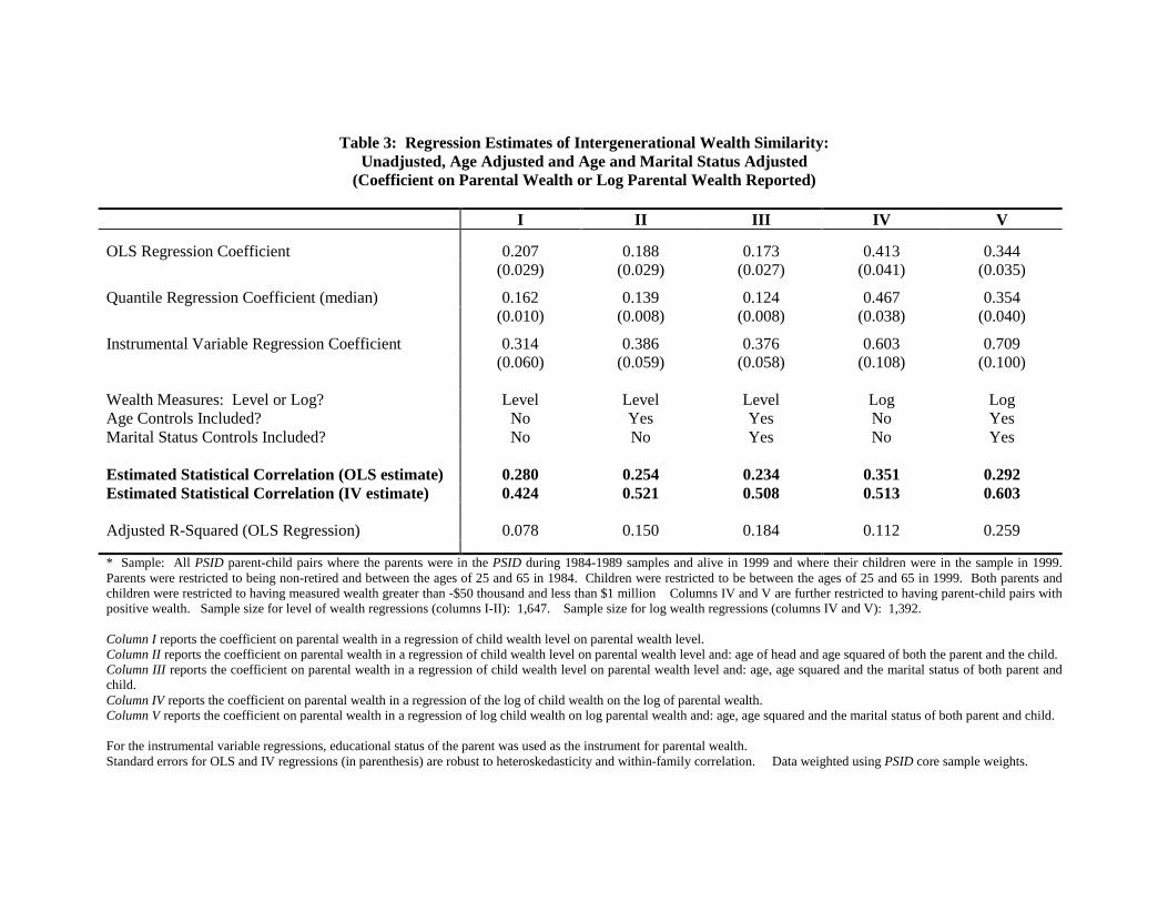
Table 3 presents the results of various regressions of the level of child wealth on the level of
parental wealth. As noted above, the independent variable is average parental wealth between 1984 and
1989, where the averaging is meant to minimize the potential classical measurement error in wealth
reporting. The child's wealth is measured in 1999, and any potential classical measurement error in the
child's wealth will be absorbed in the regression error. An OLS regression of child's wealth level in 1999
on the average parental wealth level between 1984 and 1999 (column I of Table 3) yields a coefficient on
parental wealth of 0.207 (standard error = 0.029). For every extra dollar of wealth held by a parent, the
child’s wealth is predicted to be 21 cents higher. Or, for every one dollar gap between two parents,
twenty one cents of that gap will persist between their children. Furthermore, notice that the R-squared
17
for this regression is 0.078. Almost 8 percent of the variance in child’s wealth can be explained simply
by controlling for parental wealth.
Adjusting for age and age squared of both the parent and the child (column II of Table 3) does not
change the basic results. The coefficient on parental wealth of 0.188 indicates that every extra dollar of
wealth held by a parent raises a child’s wealth by 19 cents. The second row of Table 3 shows the results
of quantile regression estimated at the median of child’s wealth on parental wealth. The estimated
persistence at the median is slightly lower in both cases. Focusing on the age adjusted results, a one
dollar increase in parental wealth increases the child’s wealth by 14.9 cents. The results also change
little when controls for the parents’ and the child’s marital status are added (column III of Table 3).
The OLS and median regression coefficients on parental wealth are, respectively, 0.173 and 0.124 (p-
values = 0.000 for both).
As noted above, the results above may be downwards biased because of measurement error in
parental wealth. Using average parental wealth over multiple years minimizes this problem, but need not
totally eliminate it. We further deal with the measurement error concern by instrumenting for parental
wealth using the parent's level of educational attainment. The educational level of a household has
strong predictive power for household wealth, even when other demographic controls and income are
included in the specification.16 An obvious shortcoming of this approach is that educational attainment
may have an independent effect on household wealth accumulation. Children from higher educated
households may be more financially sophisticated and, as a result, may be more likely to accumulate
wealth when compared to otherwise identical children from less-educated families. The estimate from
an IV regression with parental educational attainment as an instrument for parental wealth will, as a
result, possibly be biased upwards. However, the OLS estimate and the IV estimate should provide
lower and upper bounds on the true correlation between parental and child wealth.17 The IV estimate of
the correlation between parental and child wealth in the age adjusted specification is 0.386, providing a
range for the true estimate of between 0.188 and 0.386.
How do these numbers compare to the income correlations found in the literature? Many authors
who focus on the intergeneration similarity in income do not report the intergenerational correlation in
income but, instead, report the intergenerational income elasticity - i.e., the coefficient on log parental
income in a regression of log child income on log parental income and age controls. Using the mean
wealth levels given in Table 1a and using the estimated OLS coefficient from Table 3, we can compute a
16 See Hurst, Luoh and Stafford (1998) for results on the role of education in household wealth accumulation using PSIDwealth data from 1989 and 1994. In our specification, we control for education by including two dummy variables: whether thehousehold head had less than a high school education and whether the household head had exactly 12 years of schooling. Theomitted category was whether the household head had more than a high school education.17 The use of educational attainment as an instrument for parental income is a common technique used in the literature whichcalculates the intergenerational correlation in income. For an example, see Solon (1992) or Mulligan (1997).
18
similar intergenerational elasticity at the mean for wealth. The ratio of mean wealth for parents and
children is 2.03. Converting the OLS estimate to an elasticity, we find that a 1% increase in parental
wealth corresponds to a 0.35% increase in child wealth.18 Using the OLS and IV estimates, we compute
a range of intergenerational wealth elasticities between 0.35 and 0.76 - similar to the range of
intergenerational income elasticities reported in the survey by Solon (1999).19
We also estimate the correlation in child log wealth and parent log wealth on the portion of the
analysis sample where both the parent and the child have positive wealth. These regression results using
log wealth, and with and without demographic controls, are reported in columns IV and V, respectively,
of Table 3. The results are quite similar to the income elasticity documented in the literature and the
intergenerational wealth elasticity documented above (0.34 (OLS) - 0.71 (IV), column V of Table 3).
The range of elasticities reported by Mulligan (1997) using PSID data from an early time period also
falls within the range of elasticities we report.
As discussed in Section III, the estimated coefficient on parental wealth using either level or log
wealth is not a true estimate of the “statistical correlation” between parental and child wealth. The
regression coefficient estimate is only an estimate of the statistical correlation when the standard
deviations of parental and child wealth are equal to each other. As seen in Table 1a, this is not the case
with parental and child wealth in the sample. To compute an estimate of the statistical correlation in
wealth across parents and their children, we adjust the coefficient on parental wealth in the regressions
reported in Table 3 by the ratio of the standard deviation of parental wealth to the standard deviation of
child wealth. From Table 1a, this ratio is 1.35, implying an estimated intergenerational statistical wealth
correlation in the range of 0.23 (OLS specification) to 0.50 (IV specification), using the regression
results from column III of Table 3. The ratio of the standard deviation of log wealth is 0.85 resulting in
an estimated intergenerational statistical wealth correlation in the range of 0.29 (OLS) to 0.60 (IV), using
the regression results from column V of Table 3. Again, the results match rather well those found by
Zimmerman (1992) who found estimates of the intergenerational statistical correlation in income to be in
the range of 0.30 to 0.50.
The results in this section reveal that there is a strong intergenerational similarity in financial
wealth. The magnitude of the correlation is similar to that found by researchers who have estimated the
intergenerational income correlation. In section III, we set out a simple life cycle model in which the
18 The elasticity was computed as the coefficient of parental wealth in regression III of table 3 multiplied by the ratio of themeans of parental wealth to child wealth. For our OLS specification with age and marital status controls, we get 0.173 * 2.03 =0.351.19 Regressing log average child income on log average parental income and age controls, Solon (1991) estimates a coefficienton log parental income in the range of 0.41 (OLS) to 0.53 (IV). Zimmerman (1991) estimates the elasticity to be in the range of0.30 (OLS) to 0.50 (IV), while Mulligan (1997) finds estimates in the range of 0.33 (OLS) and 0.53 (IV). Using a similarapproach on our data, we find that the elasticity in log average family income between parents and their children was in a rangeof 0.36 (OLS) to 0.60 (IV).
19
correlation in wealth is, at least, partially determined by the intergenerational correlation in income. To
what extent does similarity in permanent income across parents and their children explain the similarity
in wealth across parents and their children? We address this question in the next section.
VI. The Effect of Income on Intergenerational Wealth Similarity
How much of the intergenerational similarity in wealth is due to the intergenerational similarity in
income? In this section, we repeat the transition matrix and regression analyses of the intergenerational
wealth correlation to account for the similarity in income between parents and their children. As shown
in section III, if the draws of endowed preferences are independent between parents and their children,
all of the wealth correlation should be explained by the income correlation. But, if parent and child
preferences are correlated (and not perfectly correlated with income), controlling for income will not
explain all of the parent-child wealth correlation.
The model assumed a measure of lifetime income for each household and that the household wealth
is measured at the end of income generating years. But the available data measures household income
and wealth at different points during the household’s working years. As a result, we neither have a full
measure of lifetime income, nor is wealth measured at the moment prior to retirement. To account for
these two facts, we use many different income controls in the analysis. We use actual earned family
labor income averaged over multiple years prior to the measurement of the household’s wealth to get a
sense of the household’s perceived permanent income.
Though not explicitly indicated in the model, current household wealth is a function not only of the
level of income, but also of expected income growth into the future. Households with a given level of
earned permanent income in the recent past but a steeper projected income profile over the near future
should be expected to have lower wealth holdings than an otherwise comparable household with a flatter
projected income profile. Additionally, precautionary theories of savings (Deaton (1991); Carroll
(1994)) also indicate that households with a larger expected variance of income, should be more likely to
accumulate wealth so as to buffer any successive draws of negative income shocks. The income
controls below account for actual level, expected lifecycle trajectory and predicted future variance.
We measure a household’s average level of labor income, as the 5-year average of family labor
income over the period of our wealth measurement for both parents and children. Parental family labor
income was averaged over the period 1983-1987 and children’s family labor income was averaged over
1992-1996.20 To calculate the household's expected lifecycle income trajectory, we used the PSID full
panel of households from 1980 to 1997 and regressed the family labor income of non-retired heads on
20 1996 income (reported in the 1997 survey) is the latest year of income that is currently available from the PSID.
20
the age of the head and age squared. We separately ran this regression for a series of occupation,
education, race, and sex cells.21 Using the coefficients on age and age squared from these regressions,
we predicted for both parents and children their expected total earned labor income between the ages of
25 and 65 and the fraction of that total income that they were predicted to have earned at their current
lifecycle position based on which of the race, sex, occupation and educational status cells the person
occupied. Households with higher expected total lifetime income and households who have earned a
larger percent of that income at their current lifecycle age should be more likely to have accumulated
greater amounts of wealth conditional on their age.
We predict expected future income variance in much the same way we computed the household’s
predicted lifecycle income trajectory. Using the full sample of PSID households, we segmented the
households into education-occupation-race-gender cells. For each of these cells, we computed the
standard deviation of income over the 1980 - 1994 period. Using the education, occupation, race and
gender of the household head for both parents and children, we applied this predicted income volatility
measure to both parents and children.
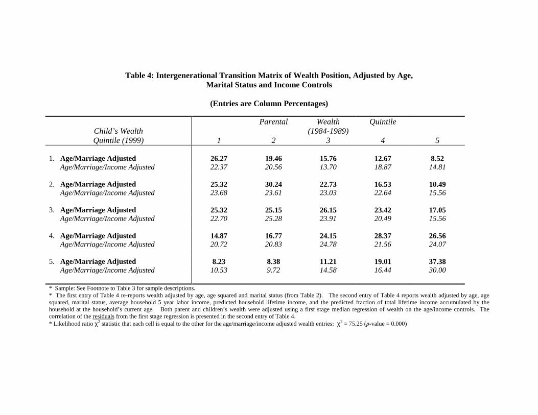
The first entry in Table 4 presents the age-marriage adjusted transition matrix reported in Table 2
(for comparison). The second entry nets out the effect of both actual income levels and predicted
lifecycle income trajectories from age-marital status adjusted wealth. That is, we regressed wealth on
age, age squared, marital status, average labor income, predicted total household earnings, and the
fraction of total earnings predicted to have been earned at the household’s current age separately for both
parents and children. Individuals are sorted into wealth quintiles based on their position in the
distribution of the residuals from these regressions. A comparison of the two estimates within any cell in
the Table 4 shows that much of the correlation in wealth position derives from correlation in actual
income levels and predicted lifecycle income trajectories.
The first interesting result is that diagonal elements of the matrix in Table 4 are much smaller after
controlling for income. The best predictor of the child’s relative wealth position is no longer their
parents relative wealth position, once income similarities are accounted for. Nonetheless, there still
appears to be some intergenerational persistence even after controlling for income. Parents in the lowest
wealth quintile remain less likely to have a child who makes it to the highest wealth quintile after
controlling for the effects of income. And, parents in the highest wealth quintile are twice as likely to
have a child who makes it to the highest wealth quintile as they are to have a child who ends up in the
lowest wealth quintile. The likelihood ratio chi squared test that all the elements of the matrix are equal 21 We used 9 occupational categories (computed by the PSID), 3 education classes (less than high school, just high school andmore than high school), black and white race cells and whether the head was male or female. In total, we estimated the expectedincome profile separately for 97 occupation-education-race-sex cells. We had less than 108 possible cells either because there
21
to 0.2 is rejected (p-value = 0.000) suggesting that some persistence still remains even after controlling
fully for income.
Table 5 shows the effect of income similarity on the absolute similarity in parent-child wealth.
Each entry is the coefficient on the parental wealth variable from a child wealth regression which include
a particular set of controls. In column I of the table, we present the age-marriage adjusted results shown
in Table 3 (for comparison) – the regression with only child and parental age, age squared and marital
status as regressors. In column II of Table 5, we add in controls for the parent’s and child’s average
family labor income. Consistent with the results in the transition matrix found in Table 4, the estimated
coefficient on parental wealth falls dramatically from 0.173 to 0.124 (a 28% reduction) in the OLS
regression. The decline in the coefficient at the median was equally dramatic - from 0.124 to 0.073 (a
41% reduction). Likewise, the IV estimate with average income as a control (using parental educational
attainment as the instrument for parental wealth) falls from 0.376 to 0.252 (a 33% reduction). After
controlling for income, the OLS, quantile and IV estimated coefficient on parental wealth still remained
strongly statistically significant, with t-values of 4.0, 8.1 and 2.8, respectively. Controlling for measures
of average household labor income explains a large portion of the intergenerational wealth correlation,
but a large statistically significant gap still remains.
Controlling for predicted total lifetime income, predicted lifecycle income trajectory and predicted
income variance do little to further explain the intergenerational wealth correlation. In column III of
Table 5, we include the households predicted total lifetime earnings and the predicted fraction of total
income earned at the household’s current age. The point estimates in column III are slightly smaller
than the point estimates in column II. The OLS coefficient on parental wealth fell from 0.124 to 0.116
with the addition of predicted lifecycle income controls. There was no effect on the quantile or the
instrumental variables regression coefficients with the additional income controls.22 Similarly, including
measures of the predicted variance of income has no additional effect on the parent-child wealth
correlation in the OLS, quantile or instrumental variables regressions (column IV of table 5).
Controlling for income fully causes the range of the point estimate on parental wealth to fall from
0.173 - 0.376 (column I) to 0.118 - 0.245 (column IV). Converting these points estimates into an
estimate of the statistical correlation, we get that the estimated correlation range falls from 0.23 (OLS) -
0.51 (IV) to 0.16 (OLS) - 0.33 (IV). Less than one-half the correlation in wealth can be explained once
controlling for income.
were no observations in some cells or because there were to few observations in these cells to run a meaningful regression. Insuch cases, some cells were grouped together.22 Including predicted lifecycle income controls in a specification without measures of average family labor income for eitherthe parent or the child causes the wealth correlation to fall from 0.173 to 0.136 in an OLS specification.
22
Including actual income earned of the parent and child essentially controls for any intergenerational
correlated “ability” which is valued by the labor market. But, households may have different levels
types of “ability” which, while correlated with wealth accumulation, are distinct from skills valued by
the labor market. To capture differences in ability between households which are uncorrelated with
income, we directly include the educational status of both the parents and children in the regression. We
are positing that there could be skills learned through education like an introduction to financial markets
which would help in wealth accumulation. Given that educational levels are correlated between parents
and their children, this financial sophistication distinct from labor market valued skills could explain part
of the parent-child wealth correlation. In column V of Table 5, we include the educational level of
parents and children in the regression specification with the full set of age, marital status and income
controls.23 Adding the educational variables has essentially no effect on the parent child wealth
correlation. In other words, education essentially has no independent effect on the intergenerational
wealth correlation once controlling for income.
Column VI of Table 5 displays the results of the effect of income and education using log parental
and child wealth. These results are consistent with the results found using the level of wealth - less than
half of the parent-child wealth correlation can be explained by the parent child income correlation.
The results in this section are mixed. As suggested by a model of wealth accumulation and life-
cycle consumption, income level, expected lifecycle income trajectory and predicted income variance do
indeed explain a non-trivial fraction of the intergenerational wealth similarity. But, fully controlling for
income accounts for less than one-half of the similarity in wealth that we document. According to the
theory outlined in section III, the simple lifecycle model with no parent-child transfers would attribute
the remaining wealth correlation to a positive correlation in preferences. In the remaining sections, we
discuss and analyze the effects of other possible explanatory factors.24
23 It should be noted that the instrumental variables specification could not be performed in column V of Table 5 since we wereusing our instrument as a regressor.24 Although not discussed in the text, we tested empirically other potential explanations for the remaining parent child wealthcorrelation. The fact that parents and child may live in the same locality may make them susceptible to similar shocks toportfolio value (in particular, housing wealth). Given that we measure parents and children 15 years apart, we are skeptical ofthis. But, if shocks are strongly persistent, such an argument could be plausible. To test for this, we included a dummy variableequal to 1 if the child currently lives in the same state as their parent into the regression reported in column V of Table 6 (bothparent and child state of residence measured in 1997). The point estimate on parental wealth remained exactly the same asreported in column V of Table 6, although the dummy variable on living in the same state did come in positive (point estimate =11,468 with a p-value of 0.106). The results were very similar if we measured parental state of residence as of 1989.Additionally, we included the total number of children of both the parent and the child (measured in 1997) as separate regressorsin a regression similar to that reported in column V of Table 6. Neither of the variables accounting for the number of children ofthe parent or the child entered significantly, nor did they impact the coefficient on parental wealth. Controlling for income andeducation likely proxies for much of the effect of family size on the wealth generating process.
23
VII. Past and Expected Parental Gifts and Intergenerational Wealth Similarity
Wealth, unlike earnings, can be directly transferred from parents to their children. We have
focused on measuring parent and child wealth prior to the giving of a bequest at the time of the parents’
death. However, as seen in section III, the expectation of a bequest can still effect the saving behavior
of both parents and children. Additionally, transfers between parents and children often times occur
before death. Although, the theoretical model abstracted from these intra-vivos gifts, we attempt to
account in the empirical specifications for such transfers during the parents’ lifetime.
We have already discussed why a bequest motive weakens the observed intergenerational wealth
correlation relative to the intergenerational income correlation. If the expected bequest was exogenous,
controlling for the expected bequest in our empirical work should actually cause the estimated
intergenerational wealth correlation to increase. This result should hold after controlling for income.
But, the expected bequest is not exogenous. As shown in section III, it is a function of both income and
endowments (including the intensity of the bequest motive) of the parents and children. Given that the
regressions already control for both parental and child income, we have already proxied for a large
portion of the expected bequest. Since the remaining portion of the expected bequest is a function of
preferences, the inclusion of a measure of expected bequest in the empirical specification may be read
acting as a control for household preferences.
The PSID, in 1994, asked respondents about their probability of leaving a bequest of $10,000 or
$100,000. No information was asked about how much of a bequest the household expected to receive.
As our measure of expected bequest, we used the max of the probability that the parent would leave a
$10,000 bequest and the probability that the parent would leave a $100,000 bequest. We adjusted the
parents’ reported expected bequest by the number of children that the parent had. This adjusted
expected bequest variable measures the amount of the bequest that could be expected to flow to a given
child.
In the sample, twenty-eight percent of all households plan to give no bequest. The median bequest
was $2,667 per child, with the mean bequest being $12,994 per child. These numbers will be lower than
aggregate statistics on the average bequests per child because the maximum bequest per child in the data
set is $100,000. We regressed the adjusted expected bequest measure on permanent income of both the
parent and the child, and age controls. As predicted by the theory, parents with higher permanent
income were statistically more likely to plan to give a bequest (coefficient = 0.166, standard error =
0.011). The coefficient on child income was also positive (coefficient = 0.038, standard error 0.012).
Older parents were more likely to plan to leave a larger bequest. The adjusted r-squared on this
regression was 0.159. As suspected, controlling for income explains a large portion of the variation in
adjusted expected bequests in the sample.
24
The results of including this adjusted expected bequest measure into the model are shown in column
I of Table 6. The specification includes the same income, education, and demographic controls as in
column V of Table 5. In the OLS regression, the coefficient on parental wealth fell, as we expect, from
0.115 to 0.106 (with a standard error of 0.030). The same result holds at the median. Accounting for
expected bequests lowers the estimated intergenerational wealth correlation.
Data from the PSID also allows us to explore the extent to which past parental gift giving explains
the remaining intergenerational wealth similarity. In 1989, 1994 and 1999, the PSID asked respondents
whether they had received a large gift of more than $10,000 during the proceeding 5 years. If so, they
asked for the amount of the gifts. This gift measure poses three potential empirical problems. First,
there is no information on gifts received before 1984. Large gifts prior to 1984 could account for wealth
similarity between parents and children in the sample, after controlling fully for income.
Second, PSID does not inquire about the source of the gift. Grandparents or a member of a spouse's
family could have been the source of the gift. This problem will likely bias us against finding a
correlation between parent's and children wealth once controlling for the gifts received. By attributing
all the of the gift giving to the parents of our parent-child pairs, we increase the children's wealth which
will, on average, explain more of the correlation than would actually be explained if we had only a
measure of parental gifts. Finally, and most importantly, we only observe gifts over $10,000. If a large
number of gifts are smaller than $10,000, especially for parents with low initial wealth, the gift measure
will not fully capture the extent of intervivos transfers between parents and their children.
Ten percent of the children in the sample received gifts in excess of $10,000 between 1984 and
1999. Gifts averaged $83,000 per gift per receiving household, with a median of $34,000. To test the
effect of gifts on the remaining correlation in wealth between parents and children, we subtracted gifts
children received during the 1984-1999 period from their 1999 wealth. Given that we measure parents
before the gift giving period (1984), we do not have to adjust parental wealth. By subtracting off gifts
received by the children we ask, in effect: What would be the intergenerational wealth if no wealth were
transferred during the parent’s lifetime?
The second column of Table 6 presents the parental wealth coefficient from a regression with child
wealth net of gifts received as the dependent variable. This adjustment makes the mean of the dependent
variable $80,000, with a standard deviation of $140,152. The regression includes the same regressors as
in the first column of Table 6. As expected, subtracting off the direct amount of intravivos transfers
lowers the observed wealth correlation. Parents are likely to give gifts when their wealth is high relative
to their children. By giving a gift, parents raise their children’s wealth, bringing it closer to theirs. The
coefficient on parental wealth in the OLS regression falls from 0.106 to 0.089.
25
Two things are of particular note from the analysis of expected bequests and actual gifts. First,
transfers from parents to children are endogenously determined. Having controlled for income directly,
accounting for these transfers likely proxies for differences in households in various preference
parameters and the extent that parents are altruistic. Second, the correlation in wealth between parents
and their children is still large and statistically different from zero (correlation = 0.12) even after
controlling for expected bequests and actual past gift giving.25
VIII. Capital Market Imperfections, Portfolio Choice and the Parent-Child WealthCorrelation
The model in Section III illustrates the role of income, intergenerational transfers and preferences in
comprising the intergenerational wealth correlation. Empirically, after controlling for income and
transfers, a sizeable correlation in wealth persists between parents and their children. Can we conclude
that the remaining similarity in savings is due to a similarity in preferences? Or, is it that imperfections
in capital markets can explain the remaining wealth correlation? In this section, we explore these
questions.
Portfolio Composition and the Parent-Child Wealth Correlation
There are two reasons why incomplete capital markets may explain the remaining intergenerational
wealth correlation. First, parents with high wealth are better able to assist their children in the face of
unfortunate events. One such event could be the financial loss suffered in a risky financial investment
which turns out badly. That is, wealthy parents may provide wealth insurance to their children against
the down-side risk from risky investments. As a result, children of these parents may be more likely to
undertake such investments, with possible positive effects on their wealth as a result. Second, wealthy
parents may be better able to relax the liquidity constraints faced by their children in market transactions.
Large fixed costs present in accessing certain portfolio components (housing, stocks, business) may
otherwise prevent children from holding their wealth in these forms (See Engelhardt (1996), Charles and
Hurst (2001), and Vissing-Jorgenson (2000)). Wealthy parents may be able to help children overcome
these financial constraints.
Our attempt to assess the role of imperfect capital markets on the large remaining parent-child
wealth correlation is broken into two steps. First, we explore whether the child’s portfolio choice
reduces the remaining intergenerational wealth correlation. We then attempt to determine whether the
systematic relationship between the child’s portfolio choice and parental wealth is explained by
imperfect capital markets, or by shared preferences and learned behavior. 25 The correlation is the coefficient on parental wealth (0.089) multiplied by the ratio of the standard deviation of parental
26
A simple way to assess whether the portfolio choices made by children are in fact related to
parental wealth, and the effect this has on the intergenerational wealth correlation is to include indicators
of a child’s ownership of risky assets to the regression reported in column II of Table 6. We explore two
risky portfolio choices of the child: stock ownership and business ownership. The first column of Table 7
includes an indicator variable for whether the child owns stocks into the regression of child wealth net of
gifts received specified in column II of Table 6. The inclusion of the stock ownership variable reduces
the coefficient on parental wealth from 0.089 to 0.081 (standard error = 0.030). Column II of Table 7
adds a binary variable for whether a child owns a business as separate indicator of a risky investment
decision to the regression specified in column one. The estimated coefficient falls even further (to 0.068,
standard error 0.028), in the OLS regression with the addition of the business ownership dummy.
Overall, adding proxies for risky financial actions on the part of the child causes the parental wealth
coefficient to fall by about an additional 22% (from 0.089 to 0.068). It should be noted that even with
the inclusion of the portfolio choice components the remaining statistical intergenerational wealth
correlation remains positive and statistically different from zero (correlation = 0.09, standard error =
0.04).
These results in Table 7 indicate that children of wealthy parents engage in riskier financial
decisions. But as alluded to above, neither the insurance nor liquidity argument need be the reason for
this. Parental wealth levels could be related to the investment decisions made by children because
wealthy parents may have provided environments in which children may be more likely to learn about or
value particular types of investment actions. Or, it could be that parents are wealthy because of their
own willingness to take high-risk, but high-yield, investment actions. Because of biological inheritance
alone, the children of such parents may themselves be quite likely to possess whatever character traits
raise the odds of investment in risky financial vehicles. The next section explores the extent to which the
portfolio composition indicators proxy for unmeasured shared endowments, rather than for the insurance
effects discussed above.
The Correlation of Portfolio Choice Across Generations
To what extent does the effect of portfolio component ownership on the wealth correlation indicate
shared endowments such as financial human capital, or risk preferences, between parents and their
children? Notice that the arguments that parents provide insurance or ease liquidity constraints suggest
that it is the level of parental wealth which is important to the child’s portfolio decision; how parental
wealth is held should be relatively unimportant. On the other hand, similar endowments between
wealth to child’s wealth net of gifts ($187,502/$140,152 = 1.34).
27
parent and child would mean that the portfolio decisions of parents affect the portfolio decisions of
children, regardless of the level of parental wealth.
Table 8 reports the result of whether children entered into different portfolio components between
1989 and 1999 as a function of their own wealth in 1989, their parents’ average wealth between 1984
and 1989, and their parents’ portfolio decision as of 1984.26 The regressions also control for age,
demographic and income controls of the child. We find a number of interesting results. First, whether
the child enters a business is positively affected by whether parents had made the same decision many
years before. Children of parents who owned a business were 7.4 percentage points more likely to
become a business owner as compared to children of parents who did not own a business. Since the
average probability of entering into business ownership was 0.155, this represents an increase of 45.2%.
Second, the effect of parents own portfolio decisions is not evident with child stock ownership entry.27
Third, the level of parental wealth is independently important for whether a child enters the stock market
but it is not independently important for whether the child owns a business.28 Finally, the child’s own
wealth as of 1989 is not important for either the decision to become a business or stock owner.
The results lend credence to the interfamily insurance hypothesis discussed above, as far as entry
into stock ownership is concerned. Children of wealthy parents may be more likely to invest in the
stock market if they know that their parents could bail them out if ever they realized a low (or negative)
realized return. Oddly, this result is not reproduced for entry into business ownership - a very risky
venture. Children of business owners are much more likely to become business owners, regardless of
parental wealth, if their parent is a business owner. This suggests that there could be another role played
by the family (learning of entrepreneurial skills, family obligation, similarity in risk preferences) that
lend itself to business ownership being propagated across generations.
The analysis indicates that portfolios are similar between parents and children, independent of the
level of the parental wealth (at least for business ownership). Are similar preferences or financial
26 The analysis in Table 8 differs from that in the main sample of analysis in that we focus on the decisions that the childrenmade over the ten year period between 1989 and 1999 rather than their decisions at one point in time (i.e., 1999). Focusing onthe change in behavior accounts for any potential endogeniety between child wealth and child portfolio component. The samplesizes in Table 8 differ from that of our main sample analysis for two reasons. First, we impose that children be in the sample asof 1989 – requirement which meant that children who had not yet formed their own households in 1989 were dropped from themain sample. Second, we analyze households who had not owned the particular portfolio component as of 1989 and analyzewhether these households transitioned into the portfolio component as of 1999.27 Chiteji and Stafford (2000) also test for relationship in stock ownership propensities between parents and children, and reporta weak correlation between these decisions. Our tests differ from their for a number of reasons. First, we examine thetransition into stock ownership rather than the relationship in the level. Also, unlike Chiteji and Stafford, we control for parentalwealth in the child stock ownership decision. We believe that this second difference principally explains why they find anintergenerational correlation and we do not.28 These results are consistent with much existing empirical literature on business ownership. Hurst and Lusardi (2000) showthat liquidity constraints are not important in business ownership. Yet, they find that parental business ownership is a strongpredictor of a child’s business ownership. The role of parental self employment as a strong statistical predictor of child’s selfemployment is robust in the literature in many samples and with the inclusion of many different controls. See Evans andLeighton (1989), Blanchflower and Oswald (1998), and Fairlie (1999) for some recent examples.
28
learning the source of this similarity? We provide further evidence for this hypothesis in the next
section.
IX. The Correlation of Preferences Across Generations?
Are preferences actually correlated between parents and their children? Both biological inheritance
and the influence of factors like financial learning or mimicry suggest that such similarity exists and, as
shown in the theoretical model, preferences certainly matter in the wealth generation process.
Unfortunately, empirically accounting for the influence of such factors is difficult. First, preferences are
likely to be highly correlated with income. Conditioning on income, therefore, would be capturing the
portion of the wealth correlation due directly to the income correlation and indirectly to the preference
correlation. Second, information on financial learning, time preference rates and risk aversion is simply
not readily available in most data sets used by economists.
In this section, we use new, experimental data from a 1996 supplement to the PSID to explore the
extent to which one specific wealth-relevant endowment measure – an index of risk tolerance - is
correlated across parents and their children.29 From a series of questions put to respondent about the
circumstances under which they would take different hypothetical gambles, PSID respondents can be
sorted into four distinct levels of risk tolerance as measured by their response to the PSID questions. We
summarize the distribution of this index, and then measure its effect on various financial choices. We
conclude with evidence on the correlation of this index between parents and children.
The PSID risk aversion measures are computed from an identical set of questions to those used by
by Barsky et. al (1997), who show that these measures predict risky household behavior by respondents
in the Health and Retirement Survey. The question in the PSID is as follows: “Suppose you had a job
that guaranteed you income for life equal to your current, total income. And that job was (your/your
family’s) only source of income. Then you are given the opportunity to take a new, and equally good
job with a 50-50 chance that it will cut your income by a third or, on the other hand, it could double your
income with a 50-50 probability. Would you take that new job?” Based on the response to that
question, the PSID asks follow-ups about jobs that double their income with a 50 percent probability or
either cut your income by, 10%, 20%, 50%, or 75% with a 50 percent probability. Assuming a CES
utility function and correcting for measurement error, the PSID reports four distinct categories of risk
aversion based on the household’s response. Barksy et. al (1997) summarize the procedure on how the
29 The risk aversion questions were only asked to PSID respondents in the 1996 survey. Furthermore, the questions were onlyput to households who were working in 1996. Our sample that is used to analyze the similarity in risk aversion is thus differentfrom the samples used in the analyses in the previous sections. Appropriate sample sizes are listed on all tables.
29
risk aversion parameters are computed using the Health and Retirement Survey data. The same
procedure was used by the PSID staff to compute the risk aversion measures using the PSID data.
Table 9a shows the distribution of risk aversion categories for both parents and children. We
classify the risk aversion measure into four categories: very high risk aversion, high risk aversion,
medium risk aversion, or low risk aversion.30 Sixty-four percent of parents and thirty-nine percent of
children fell into the very high risk aversion category.31 These households were not likely to enter a
gamble that doubled their income with a 50% probability and reduced their income by 20% with a 50%
probability. Overall, the measure suggests that parents are more risk averse than their children – a result
which is not unexpected if risk aversion increases with age.32
Table 9b measures how the risk tolerance measures affects stock and business ownership of parents
and children in the PSID. In the first column of the table, we regress parental business ownership on a
set of indicator variables denoting the risk tolerance category into which the person falls, and a series of
parental demographic and income controls. The “very high” risk aversion measure is the omitted
category. Parents with the lowest risk aversion measure were 15 percentage points more likely to own a
business (p-value - 0.000). With a base ownership rate of 0.328, this represents a 46% increase in the
probability of business ownership. Parents who are the least risk averse are most likely to engage in the
risky activity of business ownership.
Risk aversion also predicts stock ownership for parents (column II of Table 9b). Parents with the
lowest risk aversion are 13 percentage points more likely to own stocks (a 27% increase over the mean
ownership rate). The results for business ownership for children mirror the results for the parents.
Children with the highest risk aversion are the least likely to own a business. For example, children
with the lowest level of risk aversion are 7.3 percentage points more likely to own a business, an increase
of 50% over the mean child business ownership rates. With stock ownership, children with medium and
low risk aversion were also far more likely to own stocks than children with very high risk aversion,
although only the medium risk aversion group was statistically different from zero.
Table 9b suggests that, whatever its limitations, the risk tolerance parameter available in the data
appears to be related to financial choices. We turn now to the next natural question: How is this variable
related between parents and children?
30 Assuming CES preferences, the four categories (very high risk aversion, high risk aversion, medium risk aversion and lowrisk aversion) correspond to estimated risk aversion measures of 6.67, 3.57, 2.86 and 1.75, respectively. See Barsky et al (1996)for a discussion of how the risk aversion measures were calculated.31 The sample sizes for the risk aversion questions are 781 households for the parents and 1,316 households for the children.The sample size is smaller for the parents because of the large proportion of parents who were retired in 1996. The risk aversionquestions were only asked of working households.32 Although, we can not rule out cohort effects as the reason that the risk aversion measures differ between parents and theirchildren.
30
Table 10 estimates linearity probability estimates of the probability that a child is in a particular risk
tolerance category, given the category to which his parent belongs. In all of the regressions, parents in
the “very high” risk aversion category are the omitted group. The results in Panel A of Table 10 are
from a regression of child risk aversion on parental risk aversion and no other controls. The panel
indicates that substantial similarity in risk tolerance category between parents and children, especially at
the tails. Children with a very high risk aversion measure are most likely to have parents who
themselves had a very high risk aversion measure, and children with low risk aversion measures are most
likely to come from parents who had the lowest risk aversion measure. A child is 10 percentage points
more likely to have the lowest risk aversion measure if there parent had the lowest risk aversion measure
compared to if their parent the very high risk aversion measure (p-value = 0.023). This represents a
40% increase in probability over the sample mean of twenty-five percent. Notice that children with high
and medium levels of risk aversion have no statistical relationship to their parent's risk aversion measure.
The same basic pattern is evident in Panel B of the table, where the regression also controls for the
child's age, education, income status and wealth.
The results suggest that there is a strong similarity in preference parameters, especially at the tails
of the risk aversion distribution. Very risk averse parents or the least risk averse parents are likely to
have children with similar risk preferences. No such relationship holds between parents and children
with less extreme preferences. Given that portfolio components are correlated between parents and their
children (at least business ownership) regardless of parental wealth and that risk aversion measures are
correlated between parents and their children, we conclude that a correlation in endowments likely
explains part of the remaining intergenerational correlation in wealth.33
X. ConclusionEconomists and other scientists have long been interested both in the question of how economic
fortunes of children relate to those of their parents, and the reasons for any intergenerational persistence.
Most previous work in economics has limited its focus to income or earnings correlations. Furthermore,
it is well documented that there is a large amount of heterogeneity in wealth, and the failure of income
and other life cycle factors to explain that heterogeneity, suggests the possible importance of family
background in the wealth generating process. Identifying the source of this individual heterogeneity and
how it evolves across generations is an important step in more fully understanding household
consumption and saving decisions. In this paper, we assess the similarity between parents and children
33 Including the parent and child’s risk aversion measures directly into the regression reported in column V of table 5 caused thecoefficient on parental wealth to fall slightly (from 0.118 to 0.113). Of all the risk aversion measures, only the high and mediumrisk aversion measures for the child were statistically significant when the very high risk aversion measures of both the parentand the child were excluded (point estimates with t-stats in parenthesis, respectively: 17,080 (1.74) and 30,463 (2.44)).
31
in their levels of wealth holdings. We also offer suggestive evidence about the role played by
preferences - either innate or learned – in determining individual level, and study how preferences are
correlated across generations.
We begin with a simple model of the intergenerational wealth correlation. We show that knowing
the magnitude of the intergenerational income correlation tells us little about the magnitude of the
intergenerational wealth correlation. The intergenerational correlation in pre-bequest wealth can be
smaller, larger or equal to the income correlation depending on the nature of the intergenerational
correlation in preferences and the correlation between preferences and income. The standard lifecycle
model predicts that any intergenerational correlation in wealth which remains after controlling for parent
and child income and controlling directly for transfers is due to a correlation in preferences.
Using data from the PSID, we next show that there is substantial intergenerational persistence in
wealth; the raw wealth correlation between parents and their children of between 0.23 and 0.50 is similar
in magnitude to income. These intergenerational relationships are large, especially since we only focus
on households who have not yet received bequests from their parents. Controlling for measures of the
permanent income of both parents and the child only explains less than one-half of the raw
intergenerational wealth correlation. Put another way, the results indicate that if lifetime income were
completely equalized between parents whose wealth was 1 dollar apart, the gap between their children’s
wealth would only less than one-half lower than before the income equalization.
Apart from income, there are other reasons why the children of wealthy parents themselves turn out
wealthy. We find that the receipt of large gifts is not the reason: controlling for the receipt of gifts does
little to adjust the remaining correlation in wealth. On the other hand, we present results which suggest
that wealthy parents may provide insurance to their children, or that their wealth may relax their
children’s liquidity constraints. More wealth on the part of parents appears to enable children to
undertake high-risk, high return investments in corporate equities. However, investment in private
businesses seems to depend not on the level of parental wealth, but on whether the parents themselves
owned a business. Again, this suggests that for some portfolio decisions, parental characteristics aside
from parental wealth are important.
After controlling for income, demographics, education, direct transfers and portfolio composition,
we still find a sizeable and statistically significant intergenerational correlation in wealth. These controls
only explain about 60 percent of the initial age adjusted intergenerational wealth correlation. We
speculate that financial learning and shared preferences can explain a large portion of the remaining
correlation in portfolio composition and wealth levels between parents and their children. In the final
section of the paper, we present direct evidence that preferences are, in fact, correlated across
32
generations. Using experimental survey data, we show that measures of risk are strongly correlated
between parents and their children - especially at the tails of the risk aversion distribution.
One interesting area for future research is the source of this intergenerational correlation in
preferences. Our data do not permit us to distinguish whether the intergenerational similarity in
preferences derive from learning and mimicry, on the one hand, or biological transmission, on the other.
That is, we do not study here the extent to which preferences are learned and that to which they are
innate. Answering this question will further not only our understanding about the evolution of
preferences but, more generally, will further our understanding of households’ consumption and saving
decisions.
Bibliography
Altonji, Joseph, and Thomas Dunn (1991). “Relationships Among the Family Incomes andLabor Market Outcomes of Relatives.” Research in Labor Economics, 12, pgs 269-310.
Altonji, Joseph, and Thomas Dunn (2000). “An Intergenerational Model of Wages, Hours, andEarnings.” Journal of Human Resources, 35(2), pgs 221-58.
Altonji, Joseph, Fumio Hayashi, and Laurence Kotlikoff (1992). “Is the Extended FamilyAltruistically Linked? Direct Tests Using Micro Data.” American Economic Review,82(5), pgs 1177 - 98.
Barsky, Bob, Tom Juster, Miles Kimball and Matthew Shapiro (1997). “Preference Parametersand Behavioral Heterogeneity: An Experimental Approach in the Health and RetirementStudy”, Quarterly Journal of Economics, 112(2), pgs 537-79.
Becker, Gary and Nigel Tomes (1979). “An Equilibrium Theory of the Distribution of Incomeand Intergenerational Mobility.” Journal of Political Economy, 87(6), pgs 1153 - 89.
Becker, Gary and Nigel Tomes (1986). “Human Capital and the Rise and Fall of Families.”Journal of Labor Economics, 4, pgs S1-S39.
Blanchflower, David and Andrew Oswald (1998). “What Makes an Entrepreneur?” Journal ofLabor Economics, 16(1), pgs 26-59.
Carroll, Chris (1994). “How Does Future Income Affect Current Consumption.” QuarterlyJournal of Economics, 109(1), pgs 111-47.
Charles, Kerwin K. and Erik Hurst (2000). “The Transition to Home Ownership and theBlack/White Wealth Gap.” Review of Economics and Statistics (forthcoming).
Chiteji, Ngina and Frank P. Stafford (2000). “Asset Ownership Across Generations.” Universityof Michigan Working Paper.
Cox, Donald, Serena Ng and Andreas Waldkirch (2000). “Intergenerational Linkages inConsumption Behavior.” Boston College Working Paper.
Evans, David and Linda Leighton (1989). “Some Empirical Aspects of Entrepreneurship,”American Economic Review, 79(3), pgs 519 - 535.
Engelhardt, Gary (1996). “Consumption, Down Payments, and Liquidity Constraints,” Journalof Money, Credit and Banking, May, pgs 255-71.
Failrie, Robert (1999). “The Absence of African-American Owned Business: An Analysis of theDynamics of Self-Employment,” Journal of Labor Economics, 17(1), pgs 80 - 108.
Ham, Song and Casey Mulligan (2000). “Human Capital, Heterogeneity, and Estimated Degreesof Intergenerational Mobility.” NBER Working Paper No. 7678. April.
Hurst, Erik, Ming Ching Luoh, and Frank Stafford (1998). “The Wealth Dynamics of AmericanFamilies: 1984 - 1994”. Brookings Papers on Economic Activity, 98:1.
Hurst, Erik and Anna Lusardi (2000). “Entrepreneurship and Household Wealth”. UnpublishedMimeo.
Juster, Thomas, James Smith and Frank Stafford (1999). “The Measurement and Structure ofHousehold Wealth.” Labour Economics, 1999.
Kearl, James and Clayne Pope (1986). “Unobservable Family and Individual Contributions to theDistributions of Income and Wealth.” Journal of Labor Economics, 4(3) S48-79.
Menchik, Paul (1979). “Intergenerational Transmission of Inequality: An Empirical Study ofWealth Mobility.” Economica, 46(184), pgs 349-62.
Mulligan, Casey (1996). “Work Ethic and Family Background: Some Evidence’ University ofChicago Working Paper.
Mulligan, Casey (1997). Parental Priorities and Economic Inequality. University of ChicagoPress, Chicago, IL.
Samwick, Andrew (1998). “Discount Rate Heterogeneity and Social Security Reform.” Journalof Development Economics, 57, 117-146.
Solon, Gary (1992). “Intergenerational Income Mobility in the United States.” AmericanEconomic Review, 82(3), pgs 393-408.
Solon, Gary (1999). “Intergenerational Mobility in the Labor Market”, in Handbook of LaborEconomics, Volume 3, edited by Orley Ashenfelter and David Card.
Shea, John (2000). “Does Parents’ Money Matter?” Journal of Public Economics, 77, pgs 155-84.
Venti, Steven and David Wise (2000). “Choice, Chance, and Wealth Dispersion at Retirement.”NBER Working Paper No. 7521. February.
Vissing-Jorgenson, Annette (2000). “Towards an Explanation of Household Portfolio ChoiceHeterogeneity: Non-Financial Income and Participation Cost Structures.” University ofChicago Working Paper.
Wahl, Jennifer (1985). “Fertility in America: Historical Patterns and Wealth Effects on theQuantity and Quality of Children.” Ph.D. dissertation, Department of Economics,University of Chicago.
Weinberg, Bruce (2001). “An Incentive Model of the Effect of Parental Income on Children.”Journal of Political Economy, 109(2), pgs 266-80.
Zimmerman, David (1992). “Regression Toward Mediocrity in Economic Stature.” AmericanEconomic Review, 82(3), pgs 409-29.
Table 1a: Means and Standard Deviations of Wealth and Demographic Variables(1,648 Parent-Child Pairs)
Children(1999) Parents(1984-1989 average)
Variable MeanStandardDeviation Mean
StandardDeviation
Age 36.9 7.2 51.4 7.9
Marital Status 0.544 0.498 0.830 0.335
Total Number of Children 1.29 1.27 3.96 2.41
Average Family Labor Income 49,169 37,764 60,873 38,598
Wealth 84,008 139,228 170,661 187,502
% Owning Stocks 0.258 0.438 0.452 0.498
% Owning a Home 0.598 0.490 0.886 0.317
% Owning a Business 0.130 0.337 0.254 0.435
Sample: All PSID parent-child pairs where the parents were in the PSID during 1984-1989 samples and alive in 1999and where their children were in the sample in 1999. Parents were restricted to being non-retired and between the agesof 25 and 65 in 1984. Children were restricted to be between the ages of 25 and 65 in 1999. Both parents and childrenwere restricted to having measured wealth greater than -$50 thousand and less than $1 million.
Data from the core sample of the Panel Study of Income Dynamics (PSID) was used for all analyses.Wealth data came from the 1984, 1989, and 1999 PSID Wealth Supplements.All data weighted using PSID core sample weights.
Table 1b: Wealth Distribution for Children in 1999 andParents Averaged Over 1984 and 1989
* Sample: All PSID parent-child pairs where the parents were in the PSID during 1984-1989 samples and alive in1999 and where their children were in the sample in 1999. Parents were restricted to being non-retired and betweenthe ages of 25 and 65 in 1984. Children were restricted to be between the ages of 25 and 65 in 1999. Both parents andchildren were restricted to having measured wealth greater than -$50 thousand and less than $1 million (1,647observations).* The second entry reports wealth adjusted by age and age squared. Both parent and children’s wealth were adjustedusing a first stage median regression of wealth on age and age squared. The correlation of the residuals is presented inthe second entry of Table 2.* Likelihood ratio χ2 statistic that each cell is equal to the other for the unadjusted wealth entries: χ2 = 327.59 (p-value= 0.000).* Likelihood ratio χ2 statistic that each cell is equal to the other for the age adjusted wealth entries: χ2 = 292.43 (p-value = 0.000).* Likelihood ratio χ2 statistic that each cell is equal to the other for the age-marriage adjusted wealth entries: χ2 =202.6 (p-value = 0.000).
Table 3: Regression Estimates of Intergenerational Wealth Similarity:Unadjusted, Age Adjusted and Age and Marital Status Adjusted
(Coefficient on Parental Wealth or Log Parental Wealth Reported)
* Sample: All PSID parent-child pairs where the parents were in the PSID during 1984-1989 samples and alive in 1999 and where their children were in the sample in 1999.Parents were restricted to being non-retired and between the ages of 25 and 65 in 1984. Children were restricted to be between the ages of 25 and 65 in 1999. Both parents andchildren were restricted to having measured wealth greater than -$50 thousand and less than $1 million Columns IV and V are further restricted to having parent-child pairs withpositive wealth. Sample size for level of wealth regressions (columns I-II): 1,647. Sample size for log wealth regressions (columns IV and V): 1,392.
Column I reports the coefficient on parental wealth in a regression of child wealth level on parental wealth level.Column II reports the coefficient on parental wealth in a regression of child wealth level on parental wealth level and: age of head and age squared of both the parent and the child.Column III reports the coefficient on parental wealth in a regression of child wealth level on parental wealth level and: age, age squared and the marital status of both parent andchild.Column IV reports the coefficient on parental wealth in a regression of the log of child wealth on the log of parental wealth.Column V reports the coefficient on parental wealth in a regression of log child wealth on log parental wealth and: age, age squared and the marital status of both parent and child.
For the instrumental variable regressions, educational status of the parent was used as the instrument for parental wealth.Standard errors for OLS and IV regressions (in parenthesis) are robust to heteroskedasticity and within-family correlation. Data weighted using PSID core sample weights.
Table 4: Intergenerational Transition Matrix of Wealth Position, Adjusted by Age,Marital Status and Income Controls
* Sample: See Footnote to Table 3 for sample descriptions.* The first entry of Table 4 re-reports wealth adjusted by age, age squared and marital status (from Table 2). The second entry of Table 4 reports wealth adjusted by age, agesquared, marital status, average household 5 year labor income, predicted household lifetime income, and the predicted fraction of total lifetime income accumulated by thehousehold at the household’s current age. Both parent and children’s wealth were adjusted using a first stage median regression of wealth on the age/income controls. Thecorrelation of the residuals from the first stage regression is presented in the second entry of Table 4.* Likelihood ratio χ2 statistic that each cell is equal to the other for the age/marriage/income adjusted wealth entries: χ2 = 75.25 (p-value = 0.000)
Table 5: Regression Estimates of Intergenerational Wealth Similarity, Adjusting for Income
Wealth Measure: Level or Log? Level Level Level Level Level LogControls: Age and Marital Status? Yes Yes Yes Yes Yes YesControls: Actual Five Year Average Income? No Yes Yes Yes Yes YesControls: Predicted Income Trajectory? No No Yes Yes Yes YesControls: Predicted Income Volatility? No No No Yes Yes YesControls: Actual Educational Attainment? No No No No Yes No
* Sample: See Footnote to Table 3 for sample descriptions. For the instrumental variable regression, educational status of the parent was used as the instrument for parentalwealth. Standard errors for OLS and IV regressions are robust to heteroskedasticity and within-family correlation. Data weighted using PSID core sample weights.* Column I reports the coefficient on parental wealth level in a regression of child wealth level on parental wealth and: age, age squared and marital status of both the parent andthe child (re-reported from column II of Table 3).* Column II reports the coefficient on parental wealth level in a regression of child wealth on parental wealth level and: controls for age, martial status, and five-year averagehousehold labor income level for both the parent and the child.* Column III reports the coefficient on parental wealth level in a regression of child wealth level on parental wealth level and: controls for age, martial status, five-year averageincome level, and a set of controls measuring the predicted permanent income and the predicted fraction of permanent income received thus far for both the parent and the child.* Column IV reports the coefficient on parental wealth level in a regression of child wealth on parental wealth level: and the controls from regression III and measures of thepredicted income variance for both parents and the child.* Column V reports the coefficient on parental wealth in a regression of child wealth on parental wealth: and the controls from regression IV and measures of the child’s level ofeducational attainment.* Column VI reports the coefficient on log parental wealth in a regression of log child wealth on log parental wealth and the same controls from Column IV.
Table 6: Regression Estimates of Intergenerational Wealth Similarity,Adjusting for Expected Bequests and Intravivos Transfers
Adjusted R-squared from OLS Regression 0.356 0.339
* Sample: See Footnote to Table 3 for sample descriptions. Standard errors (in parenthesis) for OLS regressions arerobust to heteroskedasticity and within-family correlation. Data weighted using PSID core sample weights.
Column I reports the coefficient on parental wealth level in a regression of child’s wealth level on parental wealth leveland: age, predicted lifecycle income controls, actual average income controls, and the level of educational attainmentfor both the parent and the child and a measure of the parent’s expected bequest to the child.
Column II reports the coefficient on parental wealth level in a regression of child’s wealth level net of gifts received onparental wealth level and: age, predicted lifecycle income controls, actual average income controls, and the level ofeducational attainment for both the parent and the child and a measure of the parent’s expected bequest to the child.
Mean/Median of child’s wealth once removing gifts received from parents between 1989 and 1999: $80,000 (mean),$30,300 (median), $140,152 (standard deviation). Ratio of standard deviation of parental wealth (Table 1a) to thestandard deviation of child wealth net of transfers received is 1.34.
Table 7: Regression Estimates of Intergenerational Wealth Similarity,Adjusting for Portfolio Composition
Demographic and Income Controls Included? Yes YesExpected Bequest Control Included? Yes YesControl: Does the Child Own Stocks? Yes YesControl: Does the Child Own a Business? No Yes
Dependent Variable Child’s Wealth Net ofIntravivos Transfers
Adjusted R-squared from OLS Regression 0.376 0.417
* Sample: See Footnote to Table 3 for sample descriptions. Standard errors (in parenthesis) for OLS regressions arerobust to heteroskedasticity and within-family correlation. Data weighted using PSID core sample weights.
Column I reports the coefficient on parental wealth level in a regression of child’s wealth level net of gifts received onparental wealth level and: age, predicted lifecycle income controls, actual average income controls, the level ofeducational attainment for both the parent and the child, a measure of the parent’s expected bequest to the child and anindicator of whether the child owns stocks.
Column II reports the coefficient on parental wealth level in a regression of child’s wealth level net of gifts received onparental wealth level and: age, predicted lifecycle income controls, actual average income level controls, the level ofeducational attainment for both the parent and the child, a measure of the parent’s expected bequest to the child, anindicator of whether the child owns stocks and an indicator of whether the child owns a business.
Mean/Median of child’s wealth once removing gifts received from parents between 1989 and 1999: $80,000 (mean)and $30,300 (median)
Table 8: Linear Probability Estimates of IntergenerationalSimilarity in Portfolio Choice
ControlsEnter Stock-Ownership Enter Business-
Ownership
Parent Own Stock (1984-1989)? 0.045 0.017(0.049) (0.035)
Parent Own Business (1984-1989)? -0.001 0.069(0.060) (0.038)
* Sample: See Footnote to Table 3 for sample descriptions. Addition sample restrictions include: children wererestricted to being between ages 25 and 45 in 1999. Standard errors (in parenthesis) for the linear probabilityregressions are robust to heteroskedasticity and within-family correlation. Data weighted using PSID core sampleweights.
The dependent variable is a dummy variable indicating whether the child entered the portfolio ownership state between1989 and 1999. For example, the first column of the table has as a dependent variable whether the child became astock owner between 1989 and 1999 conditional on the child not owning stocks in 1989.
The regressions also include as regressors: the child’s age, age squared, education, average labor income, labor incomesquared and predicted lifecycle income controls.
Table 9a: The Distribution of Risk Aversion For Parents and Children
Estimated Risk Aversion Coefficient Parents Child
Very High Risk Aversion 0.640 0.389
High Risk Aversion 0.120 0.165
Medium Risk Aversion 0.084 0.195
Low Risk Aversion 0.155 0.251
* Sample: All PSID parent-child pairs where the parents were in the PSID during 1984-1989 samples and alive in1999 and where their children were in the sample in 1999. Parents were restricted to being non-retired and betweenthe ages of 25 and 65 in 1984. Children were restricted to be between the ages of 25 and 65 in 1999. Both parents andchildren were restricted to having measured wealth greater than -$50 thousand and less than $1 million. Further, forthe parent sample, the parent had to be working in 1996 (781 households). For the child sample, the child had to beworking in 1996 (1,316 households).
* Risk aversion measure from PSID 1996 Risk Aversion Supplement. See text for discussion
Table 9b: Linear Probability Estimates of Effect of Risk Aversion on HouseholdPortfolio Choice
* See note for Table 9a for a description of the sample. Results reported in Table 9b come from linear probabilityregressions of asset ownership (either stock or business) for both parents and children on their PSID risk aversionmeasures. The parents regression includes additional controls for their age, age squared, educational status, income,income squared and parameters for their expected income trajectory. Similar child specific controls were included forthe child’s regression.
Table 10: Linear Probability Estimates of Relationship Between Child and Parent RiskAversion Categories, With and Without Demographic, Income and Wealth Controls.
A. Parent-Child Risk Aversion Similarity without Demographic and Income Controls(Omitted Parental Risk Aversion Category: “Very High” Risk Aversion)
Child’s Risk Aversion MeasureRegressors Very High High Medium Low
B. Parent-Child Risk Aversion Similarity with Demographic, Income and Wealth Controls(Omitted Parental Risk Aversion Category: “Very High” Risk Aversion)
Child’s Risk Aversion MeasureRegressors Very High High Medium Low
* Samples for Panels A and B: All PSID parent-child pairs where the parents were in the PSID during 1984-1989samples and alive in 1999 and where their children were in the sample in 1999. Parents were restricted to being non-retired and between the ages of 25 and 65 in 1984. Children were restricted to be between the ages of 25 and 65 in1999. Both parents and children were restricted to having measured wealth greater than -$50 thousand and less than $1million. Furthermore, both parent and child must have been working in 1996 (see text for full discussion).* For Panel B, demographic, income and wealth controls include child’s: age, age squared, educational status, averageincome, predicted lifecycle income controls and household net wealth.