arXiv:astro-ph/0002044 v1 2 Feb 2000 The Cosmic Microwave Background Radiation Eric Gawiser 1 Department of Physics, University of California, Berkeley, CA 94720 and Joseph Silk Department of Physics, Astrophysics, 1 Keble Road, University of Oxford, OX1 3NP, UK and Departments of Physics and Astronomy and Center for Particle Astrophysics, University of California, Berkeley, CA 94720 Abstract We summarize the theoretical and observational status of the study of the Cosmic Microwave Background radiation. Its thermodynamic spectrum is a robust prediction of the Hot Big Bang cosmology and has been confirmed observationally. There are now 76 observations of Cosmic Microwave Back- ground anisotropy, which we present in a table with references. We discuss the theoretical origins of these anisotropies and explain the standard jargon associated with their observation. 1 Origin of the Cosmic Background Radiation Our present understanding of the beginning of the universe is based upon the remarkably successful theory of the Hot Big Bang. We believe that our universe began about 15 billion years ago as a hot, dense, nearly uniform sea of radiation a minute fraction of its present size (formally an infinitesimal singularity). If inflation occurred in the first fraction of a second, the universe became matter dominated while expanding exponentially and then returned to radiation domination by the reheating caused by the decay of the inflaton. Baryonic matter formed within the first second, and the nucleosynthesis of the lightest elements took only a few minutes as the universe expanded and cooled. The baryons were in the form of plasma until about 300,000 years after the Big Bang, when the universe had cooled to a temperature near 3000 K, sufficiently cool for protons to capture free electrons and form atomic hydrogen; this process is referred to as recombination. The recombination epoch occurred at 1 current address: Center for Astrophysics and Space Sciences, University of Cali- fornia at San Diego, La Jolla, CA 92037 1
Transcript
arX
iv:a
stro
-ph/
0002
044
v1
2 Fe
b 20
00
The Cosmic Microwave Background Radiation
Eric Gawiser 1
Department of Physics, University of California, Berkeley, CA 94720
andJoseph Silk
Department of Physics, Astrophysics, 1 Keble Road, University of Oxford,OX1 3NP, UK
andDepartments of Physics and Astronomy and Center for Particle
Astrophysics, University of California, Berkeley, CA 94720
Abstract
We summarize the theoretical and observational status of the study of theCosmic Microwave Background radiation. Its thermodynamic spectrum is arobust prediction of the Hot Big Bang cosmology and has been confirmedobservationally. There are now 76 observations of Cosmic Microwave Back-ground anisotropy, which we present in a table with references. We discussthe theoretical origins of these anisotropies and explain the standard jargonassociated with their observation.
1 Origin of the Cosmic Background Radiation
Our present understanding of the beginning of the universe is based uponthe remarkably successful theory of the Hot Big Bang. We believe that ouruniverse began about 15 billion years ago as a hot, dense, nearly uniform seaof radiation a minute fraction of its present size (formally an infinitesimalsingularity). If inflation occurred in the first fraction of a second, the universebecame matter dominated while expanding exponentially and then returnedto radiation domination by the reheating caused by the decay of the inflaton.Baryonic matter formed within the first second, and the nucleosynthesis of thelightest elements took only a few minutes as the universe expanded and cooled.The baryons were in the form of plasma until about 300,000 years after the BigBang, when the universe had cooled to a temperature near 3000 K, sufficientlycool for protons to capture free electrons and form atomic hydrogen; thisprocess is referred to as recombination. The recombination epoch occurred at
1 current address: Center for Astrophysics and Space Sciences, University of Cali-fornia at San Diego, La Jolla, CA 92037
1
a redshift of 1100, meaning that the universe has grown over a thousand timeslarger since then. The ionization energy of a hydrogen atom is 13.6 eV, butrecombination did not occur until the universe had cooled to a characteristictemperature (kT) of 0.3 eV (Padmanabhan, 1993). This delay had severalcauses. The high entropy of the universe made the rate of electron capture onlymarginally faster than the rate of photodissociation. Moreover, each electroncaptured directly into the ground state emits a photon capable of ionizinganother newly formed atom, so it was through recombination into excitedstates and the cooling of the universe to temperatures below the ionizationenergy of hydrogen that neutral matter finally condensed out of the plasma.Until recombination, the universe was opaque to electromagnetic radiationdue to scattering of the photons by free electrons. As recombination occurred,the density of free electrons diminished greatly, leading to the decoupling ofmatter and radiation as the universe became transparent to light.
The Cosmic Background Radiation (CBR) released during this era of decou-pling has a mean free path long enough to travel almost unperturbed untilthe present day, where we observe it peaked in the microwave region of thespectrum as the Cosmic Microwave Background (CMB). We see this radiationtoday coming from the surface of last scattering (which is really a sphericalshell of finite thickness) at a distance of nearly 15 billion light years. ThisCosmic Background Radiation was predicted by the Hot Big Bang theory anddiscovered at an antenna temperature of 3K in 1964 by Penzias & Wilson(1965). The number density of photons in the universe at a redshift z is givenby (Peebles, 1993)
nγ = 420(1 + z)3cm−3 (1)
where (1+z) is the factor by which the linear scale of the universe has expandedsince then. The radiation temperature of the universe is given by T = T0(1+z)so it is easy to see how the conditions in the early universe at high redshiftswere hot and dense.
The CBR is our best probe into the conditions of the early universe. Theoriesof the formation of large-scale structure predict the existence of slight inho-mogeneities in the distribution of matter in the early universe which under-went gravitational collapse to form galaxies, galaxy clusters, and superclusters.These density inhomogeneities lead to temperature anisotropies in the CBRdue to a combination of intrinsic temperature fluctuations and gravitationalblue/redshifting of the photons leaving under/overdense regions. The DMR(Differential Microwave Radiometer) instrument of the Cosmic BackgroundExplorer (COBE) satellite discovered primordial temperature fluctuations onangular scales larger than 7 of order ∆T/T = 10−5 (Smoot et al., 1992).Subsequent observations of the CMB have revealed temperature anisotropieson smaller angular scales which correspond to the physical scale of observed
2
structures such as galaxies and clusters of galaxies.
1.1 Thermalization
There were three main processes by which this radiation interacted with mat-ter in the first few hundred thousand years: Compton scattering, double Comp-ton scattering, and thermal bremsstrahlung. The simplest interaction of mat-ter and radiation is Compton scattering of a single photon off a free electron,γ + e− → γ + e−. The photon will transfer momentum and energy to theelectron if it has significant energy in the electron’s rest frame. However, thescattering will be well approximated by Thomson scattering if the photon’senergy in the rest frame of the electron is significantly less than the rest mass,hν ≪ mec
2. When the electron is relativistic, the photon is blueshifted byroughly a factor γ in energy when viewed from the electron rest frame, is thenemitted at almost the same energy in the electron rest frame, and is blueshiftedby another factor of γ when retransformed to the observer’s frame. Thus, ener-getic electrons can efficiently transfer energy to the photon background of theuniverse. This process is referred to as Inverse Compton scattering. The com-bination of cases where the photon gives energy to the electron and vice versaallows Compton scattering to generate thermal equilibrium (which is impossi-ble in the Thomson limit of elastic scattering). Compton scattering conservesthe number of photons. There exists a similar process, double Compton scat-tering, which produces (or absorbs) photons, e− + γ ↔ e− + γ + γ.
Another electromagnetic interaction which occurs in the plasma of the earlyuniverse is Coulomb scattering. Coulomb scattering establishes and maintainsthermal equilibrium among the baryons of the photon-baryon fluid withoutaffecting the photons. However, when electrons encounter ions they experi-ence an acceleration and therefore emit electromagnetic radiation. This iscalled thermal bremsstrahlung or free-free emission. For an ion X, we havee− + X ↔ e− + X + γ. The interaction can occur in reverse because of theability of the charged particles to absorb incoming photons; this is called free-free absorption. Each charged particle emits radiation, but the acceleration isproportional to the mass, so we can usually view the electron as being accel-erated in the fixed Coulomb field of the much heavier ion. Bremsstrahlung isdominated by electric-dipole radiation (Shu, 1991) and can also produce andabsorb photons.
The net effect is that Compton scattering is dominant for temperatures above90 eV whereas bremsstrahlung is the primary process between 90 eV and 1eV. At temperatures above 1 keV, double Compton is more efficient thanbremsstrahlung. All three processes occur faster than the expansion of theuniverse and therefore have an impact until decoupling. A static solution for
3
Compton scattering is the Bose-Einstein distribution,
fBE =1
ex+µ − 1(2)
where µ is a dimensionless chemical potential (Hu, 1995). At high opticaldepths, Compton scattering can exchange enough energy to bring the photonsto this Bose-Einstein equilibrium distribution. A Planckian spectrum corre-sponds to zero chemical potential, which will occur only when the number ofphotons and total energy are in the same proportion as they would be for ablackbody. Thus, unless the photon number starts out exactly right in compar-ison to the total energy in radiation in the universe, Compton scattering willonly produce a Bose-Einstein distribution and not a blackbody spectrum. Itis important to note, however, that Compton scattering will preserve a Planckdistribution,
fP =1
ex − 1. (3)
All three interactions will preserve a thermal spectrum if one is achieved atany point. It has long been known that the expansion of the universe servesto decrease the temperature of a blackbody spectrum,
Bν =2hν3/c2
ehν/kT − 1, (4)
but keeps it thermal (Tolman, 1934). This occurs because both the frequencyand temperature decrease as (1 + z) leaving hν/kT unchanged during ex-pansion. Although Compton scattering alone cannot produce a Planck distri-bution, such a distribution will remain unaffected by electromagnetic inter-actions or the universal expansion once it is achieved. A non-zero chemicalpotential will be reduced to zero by double Compton scattering and, later,bremsstrahlung which will create and absorb photons until the number den-sity matches the energy and a thermal distribution of zero chemical potentialis achieved. This results in the thermalization of the CBR at redshifts muchgreater than that of recombination.
Thermalization, of course, should only be able to create an equilibrium tem-perature over regions that are in causal contact. The causal horizon at thetime of last scattering was relatively small, corresponding to a scale today ofabout 200 Mpc, or a region of angular extent of one degree on the sky. How-ever, observations of the CMB show that it has an isotropic temperature onthe sky to the level of one part in one hundred thousand! This is the origin ofthe Horizon Problem, which is that there is no physical mechanism expected
4
in the early universe which can produce thermodynamic equilibrium on super-horizon scales. The inflationary universe paradigm (Guth, 1981; Linde, 1982;Albrecht & Steinhardt, 1982) solves the Horizon Problem by postulating thatthe universe underwent a brief phase of exponential expansion during the firstsecond after the Big Bang, during which our entire visible Universe expandedout of a region small enough to have already achieved thermal equilibrium.
2 CMB Spectrum
The CBR is the most perfect blackbody ever seen, according to the FIRAS(Far InfraRed Absolute Spectrometer) instrument of COBE, which measureda temperature of T0 = 2.726 ± 0.010 K (Mather et al., 1994). The theoreticalprediction that the CBR will have a blackbody spectrum appears to be con-firmed by the FIRAS observation (see Figure 1). But this is not the end ofthe story. FIRAS only observed the peak of the blackbody. Other experimentshave mapped out the Rayleigh-Jeans part of the spectrum at low frequency.Most are consistent with a 2.73 K blackbody, but some are not. It is in thelow-frequency limit that the greatest spectral distortions might occur becausea Bose-Einstein distribution differs from a Planck distribution there. However,double Compton and bremsstrahlung are most effective at low frequencies sostrong deviations from a blackbody spectrum are not generally expected.
Spectral distortions in the Wien tail of the spectrum are quite difficult to de-tect due to the foreground signal from interstellar dust at those high frequen-cies. For example, broad emission lines from electron capture at recombinationare predicted in the Wien tail but cannot be distinguished due to foregroundcontamination (White et al., 1994). However, because the energy generated bystar formation and active galactic nuclei is absorbed by interstellar dust in allgalaxies and then re-radiated in the far-infrared, we expect to see an isotropicFar-Infrared Background (FIRB) which dominates the CMB at frequenciesabove a few hundred GHz. This FIRB has now been detected in FIRAS data(Puget et al., 1996; Burigana & Popa, 1998; Fixsen et al., 1998) and in datafrom the COBE DIRBE instrument (Schlegel et al., 1998; Dwek et al., 1998).
Although Compton, double Compton, and bremsstrahlung interactions occurfrequently until decoupling, the complex interplay between them required tothermalize the CBR spectrum is ineffective at redshifts below 107. This meansthat any process after that time which adds a significant portion of energy tothe universe will lead to a spectral distortion today. Neutrino decays duringthis epoch should lead to a Bose-Einstein rather than a Planck distribution,and this allows the FIRAS observations to set constraints on the decay ofneutrinos and other particles in the early universe (Kolb & Turner, 1990).The apparent impossibility of thermalizing radiation at low redshift makes
5
Fig. 1. Measurements of the CMB spectrum.
the blackbody nature of the CBR strong evidence that it did originate in theearly universe and as a result serves to support the Big Bang theory.
The process of Compton scattering can cause spectral distortions if it is toolate for double Compton and bremsstrahlung to be effective. In general, low-frequency photons will be shifted to higher frequencies, thereby decreasingthe number of photons in the Rayleigh-Jeans region and enhancing the Wientail. This is referred to as a Compton-y distortion and it is described by theparameter
y =∫
Te(t)
meσne(t)dt. (5)
The apparent temperature drop in the long-wavelength limit is
δT
T= −2y. (6)
The most important example of this is Compton scattering of photons off hotelectrons in galaxy clusters, called the Sunyaev-Zel’dovich (SZ) effect. Theelectrons transfer energy to the photons, and the spectral distortion resultsfrom the sum of all of the scatterings off electrons in thermal motion, each ofwhich has a Doppler shift. The SZ effect from clusters can yield a distortion
6
of y ≃ 10−5 − 10−3 and these distortions have been observed in several richclusters of galaxies. The FIRAS observations place a constraint on any full-sky Comptonization by limiting the average y-distortion to y < 2.5 × 10⁻⁵
(Hu, 1995). The integrated y-distortion predicted from the SZ effect of galaxyclusters and large-scale structure is over a factor of ten lower than this obser-vational constraint (Refregier et al., 1998) but that from “cocoons” of radiogalaxies (Yamada et al., 1999) is predicted to be of the same order. A kine-matic SZ effect is caused by the bulk velocity of the cluster; this is a smalleffect which is very difficult to detect for individual clusters but will likely bemeasured statistically by the Planck satellite.
3 CMB Anisotropy
The temperature anisotropy at a point on the sky (θ, φ) can be expressed inthe basis of spherical harmonics as
∆T
T(θ, φ) =
∑
ℓm
aℓmYℓm(θ, φ). (7)
A cosmological model predicts the variance of the aℓm coefficients over anensemble of universes (or an ensemble of observational points within one uni-verse, if the universe is ergodic). The assumptions of rotational symmetryand Gaussianity allow us to express this ensemble average in terms of themultipoles Cℓ as
〈a∗
ℓmaℓ′m′〉 ≡ Cℓδℓ′ℓδm′m. (8)
The predictions of a cosmological model can be expressed in terms of Cℓ aloneif that model predicts a Gaussian distribution of density perturbations, inwhich case the aℓm will have mean zero and variance Cℓ.
The temperature anisotropies of the CMB detected by COBE are believedto result from inhomogeneities in the distribution of matter at the epoch ofrecombination. Because Compton scattering is an isotropic process in the elec-tron rest frame, any primordial anisotropies (as opposed to inhomogeneities)should have been smoothed out before decoupling. This lends credence to theinterpretation of the observed anisotropies as the result of density pertur-bations which seeded the formation of galaxies and clusters. The discoveryof temperature anisotropies by COBE provides evidence that such densityinhomogeneities existed in the early universe, perhaps caused by quantumfluctuations in the scalar field of inflation or by topological defects resultingfrom a phase transition (see Kamionkowski & Kosowsky, 1999 for a detailed
7
review of inflationary and defect model predictions for CMB anisotropies).Gravitational collapse of these primordial density inhomogeneities appears tohave formed the large-scale structures of galaxies, clusters, and superclustersthat we observe today.
On large (super-horizon) scales, the anisotropies seen in the CMB are producedby the Sachs-Wolfe effect (Sachs & Wolfe, 1967).
(
∆T
T
)
SW= v · e|eo − Φ|eo +
1
2
e∫
o
hρσ,0nρnσdξ, (9)
where the first term is the net Doppler shift of the photon due to the relativemotion of emitter and observer, which is referred to as the kinematic dipole.This dipole, first observed by Smoot et al. (1977), is much larger than otherCMB anisotropies and is believed to reflect the motion of the Earth relativeto the average reference frame of the CMB. Most of this motion is due to thepeculiar velocity of the Local Group of galaxies. The second term representsthe gravitational redshift due to a difference in gravitational potential betweenthe site of photon emission and the observer. The third term is called the In-tegrated Sachs-Wolfe (ISW) effect and is caused by a non-zero time derivativeof the metric along the photon’s path of travel due to potential decay, gravi-tational waves, or non-linear structure evolution (the Rees-Sciama effect). Ina matter-dominated universe with scalar density perturbations the integralvanishes on linear scales. This equation gives the redshift from emission toobservation, but there is also an intrinsic ∆T/T on the last-scattering sur-face due to the local density of photons. For adiabatic perturbations, we have(White & Hu, 1997) an intrinsic
∆T
T=
1
3
δρ
ρ=
2
3Φ. (10)
Putting the observer at Φ = 0 (the observer’s gravitational potential merelyadds a constant energy to all CMB photons) this leads to a net Sachs-Wolfeeffect of ∆T/T = −Φ/3 which means that overdensities lead to cold spots inthe CMB.
3.1 Small-angle anisotropy
Anisotropy measurements on small angular scales (0.1 to 1) are expectedto reveal the so-called first acoustic peak of the CMB power spectrum. Thispeak in the anisotropy power spectrum corresponds to the scale where acousticoscillations of the photon-baryon fluid caused by primordial density inhomo-
8
Fig. 2. Dependence of CMB anisotropy power spectrum on cosmological parameters.
geneities are just reaching their maximum amplitude at the surface of lastscattering i.e. the sound horizon at recombination. Further acoustic peaks oc-cur at scales that are reaching their second, third, fourth, etc. antinodes ofoscillation.
Figure 2 (from Hu et al., 1997) shows the dependence of the CMB anisotropypower spectrum on a number of cosmological parameters. The acoustic oscil-lations in density (light solid line) are sharp here because they are really beingplotted against spatial scales, which are then smoothed as they are projectedthrough the last-scattering surface onto angular scales. The troughs in thedensity oscillations are filled in by the 90-degree-out-of-phase velocity oscilla-tions (this is a Doppler effect but does not correspond to the net peaks, whichare best referred to as acoustic peaks rather than Doppler peaks). The origin
9
of this plot is at a different place for different values of the matter densityand the cosmological constant; the negative spatial curvature of an open uni-verse makes a given spatial scale correspond to a smaller angular scale. TheIntegrated Sachs-Wolfe (ISW) effect occurs whenever gravitational potentialsdecay due to a lack of matter dominance. Hence the early ISW effect occursjust after recombination when the density of radiation is still considerableand serves to broaden the first acoustic peak at scales just larger than thehorizon size at recombination. And for a present-day matter density less thancritical, there is a late ISW effect that matters on very large angular scales -it is greater in amplitude for open universes than for lambda-dominated be-cause matter domination ends earlier in an open universe for the same valueof the matter density today. The late ISW effect should correlate with large-scale structures that are otherwise detectable at z ∼ 1, and this allows theCMB to be cross-correlated with observations of the X-ray background to de-termine Ω (Crittenden & Turok, 1996; Kamionkowski, 1996; Boughn et al.,1998; Kamionkowski & Kinkhabwala, 1999) or with observations of large-scalestructure to determine the bias of galaxies (Suginohara et al., 1998).
For a given model, the location of the first acoustic peak can yield informationabout Ω, the ratio of the density of the universe to the critical density needed tostop its expansion. For adiabatic density perturbations, the first acoustic peakwill occur at ℓ = 220Ω−1/2 (Kamionkowski et al., 1994). The ratio of ℓ valuesof the peaks is a robust test of the nature of the density perturbations; foradiabatic perturbations these will have ratio 1:2:3:4 whereas for isocurvatureperturbations the ratio should be 1:3:5:7 (Hu & White, 1996). A mixtureof adiabatic and isocurvature perturbations is possible, and this test shouldreveal it.
As illustrated in Figure 2, the amplitude of the acoustic peaks depends on thebaryon fraction Ωb, the matter density Ω0, and Hubble’s constant H0 = 100hkm/s/Mpc. A precise measurement of all three acoustic peaks can reveal thefraction of hot dark matter and even potentially the number of neutrino species(Dodelson et al., 1996). Figure 2 shows the envelope of the CMB anisotropydamping tail on arcminute scales, where the fluctuations are decreased due tophoton diffusion (Silk, 1967) as well as the finite thickness of the last-scatteringsurface. This damping tail is a sensitive probe of cosmological parameters andhas the potential to break degeneracies between models which explain thelarger-scale anisotropies (Hu & White, 1997b; Metcalf & Silk, 1998). The
characteristic angular scale for this damping is given by 1.8′Ω−1/2
B Ω3/4
0 h−1/2
(White et al., 1994).
There is now a plethora of theoretical models which predict the developmentof primordial density perturbations into microwave background anisotropies.These models differ in their explanation of the origin of density inhomo-geneities (inflation or topological defects), the nature of the dark matter (hot,
10
cold, baryonic, or a mixture of the three), the curvature of the universe (Ω),the value of the cosmological constant (Λ), the value of Hubble’s constant,and the possibility of reionization which wholly or partially erased tempera-ture anisotropies in the CMB on scales smaller than the horizon size. Availabledata does not allow us to constrain all (or even most) of these parameters,so analyzing current CMB anisotropy data requires a model-independent ap-proach. It seems reasonable to view the mapping of the acoustic peaks as ameans of determining the nature of parameter space before going on to fittingcosmological parameters directly.
3.2 Reionization
The possibility that post-decoupling interactions between ionized matter andthe CBR have affected the anisotropies on scales smaller than those measuredby COBE is of great significance for current experiments. Reionization is in-evitable but its effect on anisotropies depends significantly on when it occurs(see Haimann & Knox, 1999 for a review). Early reionization leads to a largeroptical depth and therefore a greater damping of the anisotropy power spec-trum due to the secondary scattering of CMB photons off of the newly freeelectrons. For a universe with critical matter density and constant ionizationfraction xe, the optical depth as a function of redshift is given by (White et al.,1994)
τ ≃ 0.035ΩBhxez3/2, (11)
which allows us to determine the redshift of reionization z∗ at which τ = 1,
z∗ ≃ 69
(
h
0.5
)
−2
3(
ΩB
0.1
)−2
3
x−
2
3e Ω
1
3 , (12)
where the scaling with Ω applies to an open universe only. At scales smallerthan the horizon size at reionization, ∆T/T is reduced by the factor e−τ .
Attempts to measure the temperature anisotropy on angular scales of less thana degree which correspond to the size of galaxies could have led to a surprise;if the universe was reionized after recombination to the extent that the CBRwas significantly scattered at redshifts less than 1100, the small-scale primor-dial anisotropies would have been washed out. To have an appreciable opticaldepth for photon-matter interaction, reionization cannot have occurred muchlater than a redshift of 20 (Padmanabhan, 1993). Large-scale anisotropies suchas those seen by COBE are not expected to be affected by reionization be-cause they encompass regions of the universe which were not yet in causal
11
contact even at the proposed time of reionization. However, the apparentlyhigh amplitiude of degree-scale anisotropies is a strong argument against thepossibility of early (z ≥ 50) reionization. On arc-minute scales, the interactionof photons with reionized matter is expected to have eliminated the primor-dial anisotropies and replaced them with smaller secondary anisotropies fromthis new surface of last scattering (the Ostriker-Vishniac effect and patchyreionization, see next section).
3.3 Secondary Anisotropies
Secondary CMB anisotropies occur when the photons of the Cosmic MicrowaveBackground radiation are scattered after the original last-scattering surface(see Refregier, 1999 for a review). The shape of the blackbody spectrumcan be altered through inverse Compton scattering by the thermal Sunyaev-Zel’dovich (SZ) effect (Sunyaev & Zeldovich, 1972). The effective temperatureof the blackbody can be shifted locally by a doppler shift from the peculiarvelocity of the scattering medium (the kinetic SZ and Ostriker-Vishniac ef-fects, Ostriker & Vishniac, 1986) as well as by passage through the changinggravitational potential caused by the collapse of nonlinear structure (the Rees-Sciama effect, Rees & Sciama, 1968) or the onset of curvature or cosmologicalconstant domination (the Integrated Sachs-Wolfe effect). Several simulationsof the impact of patchy reionization have been performed (Aghanim et al.,1996; Knox et al., 1998; Gruzinov & Hu, 1998; Peebles & Juszkiewicz, 1998).The SZ effect itself is independent of redshift, so it can yield information onclusters at much higher redshift than does X-ray emission. However, nearlyall clusters are unresolved for 10′ resolution so higher-redshift clusters occupyless of the beam and therefore their SZ effect is in fact dimmer. In the 4.5′
channels of Planck this will no longer be true, and the SZ effect can probecluster abundance at high redshift. An additional secondary anisotropy is thatcaused by gravitational lensing (see e.g. Cayon et al., 1993, 1994; Metcalf &Silk, 1997; Martinez-Gonzalez et al., 1997). Gravitational lensing imprintsslight non-Gaussianity in the CMB from which it might be possible to deter-mine the matter power spectrum (Seljak & Zaldarriaga, 1998; Zaldarriaga &Seljak, 1998).
3.4 Polarization Anisotropies
Polarization of the Cosmic Microwave Background radiation (Kosowsky, 1994;Kamionkowski et al., 1997; Zaldarriaga & Seljak, 1997) arises due to localquadrupole anisotropies at each point on the surface of last scattering (see Hu& White, 1997a for a review). Scalar (density) perturbations generate curl-
12
free (electric mode) polarization only, but tensor (gravitational wave) pertur-bations can generate divergence-free (magnetic mode) polarization. Hence thepolarization of the CMB is a potentially useful probe of the level of gravita-tional waves in the early universe (Seljak & Zaldarriaga, 1997; Kamionkowski& Kosowsky, 1998), especially since current indications are that the large-scaleprimary anisotropies seen by COBE do not contain a measurable fraction oftensor contributions (Gawiser & Silk, 1998). A thorough review of gravitywaves and CMB polarization is given by Kamionkowski & Kosowsky (1999).
3.5 Gaussianity of the CMB anisotropies
The processes turning density inhomogeneities into CMB anisotropies are lin-ear, so cosmological models that predict gaussian primordial density inhomo-geneities also predict a gaussian distribution of CMB temperature fluctuations.Several techniques have been developed to test COBE and future datasets fordeviations from gaussianity (e.g. Kogut et al., 1996b; Ferreira & Magueijo,1997; Ferreira et al., 1997). Most tests have proven negative, but a few claimsof non-gaussianity have been made. Gaztanaga et al. (1998) found a verymarginal indication of non-gaussianity in the spread of results for degree-scaleCMB anisotropy observations being greater than the expected sample vari-ances. Ferreira et al. (1998) have claimed a detection of non-gaussianity atmultipole ℓ = 16 using a bispectrum statistic, and Pando et al. (1998) find anon-gaussian wavelet coefficient correlation on roughly 15 scales in the NorthGalactic hemisphere. Both of these methods produce results consistent withgaussianity, however, if a particular area of several pixels is eliminated fromthe dataset (Bromley & Tegmark, 1999). A true sky signal should be largerthan several pixels so instrument noise is the most likely source of the non-gaussianity. A different area appears to cause each detection, giving evidencethat the COBE dataset had non-gaussian instrument noise in at least twoareas of the sky.
3.6 Foreground contamination
Of particular concern in measuring CMB anisotropies is the issue of fore-ground contamination. Foregrounds which can affect CMB observations in-clude galactic radio emission (synchrotron and free-free), galactic infraredemission (dust), extragalactic radio sources (primarily elliptical galaxies, ac-tive galactic nuclei, and quasars), extragalactic infrared sources (mostly dustyspirals and high-redshift starburst galaxies), and the Sunyaev-Zel’dovich effectfrom hot gas in galaxy clusters. The COBE team has gone to great lengths toanalyze their data for possible foreground contamination and routinely elimi-
13
nates everything within about 30 of the galactic plane.
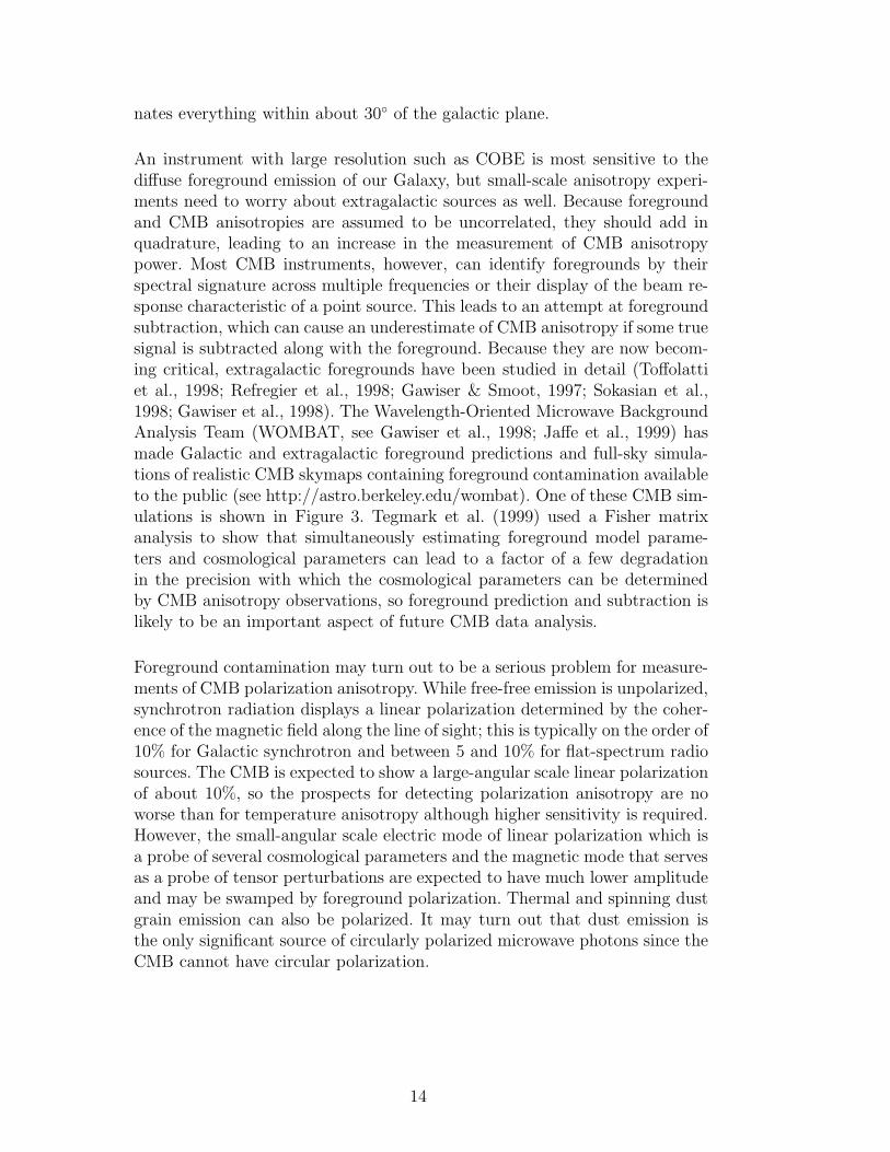
An instrument with large resolution such as COBE is most sensitive to thediffuse foreground emission of our Galaxy, but small-scale anisotropy experi-ments need to worry about extragalactic sources as well. Because foregroundand CMB anisotropies are assumed to be uncorrelated, they should add inquadrature, leading to an increase in the measurement of CMB anisotropypower. Most CMB instruments, however, can identify foregrounds by theirspectral signature across multiple frequencies or their display of the beam re-sponse characteristic of a point source. This leads to an attempt at foregroundsubtraction, which can cause an underestimate of CMB anisotropy if some truesignal is subtracted along with the foreground. Because they are now becom-ing critical, extragalactic foregrounds have been studied in detail (Toffolattiet al., 1998; Refregier et al., 1998; Gawiser & Smoot, 1997; Sokasian et al.,1998; Gawiser et al., 1998). The Wavelength-Oriented Microwave BackgroundAnalysis Team (WOMBAT, see Gawiser et al., 1998; Jaffe et al., 1999) hasmade Galactic and extragalactic foreground predictions and full-sky simula-tions of realistic CMB skymaps containing foreground contamination availableto the public (see http://astro.berkeley.edu/wombat). One of these CMB sim-ulations is shown in Figure 3. Tegmark et al. (1999) used a Fisher matrixanalysis to show that simultaneously estimating foreground model parame-ters and cosmological parameters can lead to a factor of a few degradationin the precision with which the cosmological parameters can be determinedby CMB anisotropy observations, so foreground prediction and subtraction islikely to be an important aspect of future CMB data analysis.
Foreground contamination may turn out to be a serious problem for measure-ments of CMB polarization anisotropy. While free-free emission is unpolarized,synchrotron radiation displays a linear polarization determined by the coher-ence of the magnetic field along the line of sight; this is typically on the order of10% for Galactic synchrotron and between 5 and 10% for flat-spectrum radiosources. The CMB is expected to show a large-angular scale linear polarizationof about 10%, so the prospects for detecting polarization anisotropy are noworse than for temperature anisotropy although higher sensitivity is required.However, the small-angular scale electric mode of linear polarization which isa probe of several cosmological parameters and the magnetic mode that servesas a probe of tensor perturbations are expected to have much lower amplitudeand may be swamped by foreground polarization. Thermal and spinning dustgrain emission can also be polarized. It may turn out that dust emission isthe only significant source of circularly polarized microwave photons since theCMB cannot have circular polarization.
Fig. 3. WOMBAT Challenge simulation of CMB anisotropy map that might be ob-served by the MAP satellite at 90 GHz, 13’ resolution, containing CMB, instrumentnoise, and foreground contamination. The resolution is degraded by the pixelizationof your monitor or printer.
Since the COBE DMR detection of CMB anisotropy (Smoot et al., 1992),there have been over thirty additional measurements of anisotropy on angularscales ranging from 7 to 0.3, and upper limits have been set on smaller scales.
The COBE DMR observations were pixelized into a skymap, from which itis possible to analyze any particular multipole within the resolution of theDMR. Current small angular scale CMB anisotropy observations are insensi-tive to both high ℓ and low ℓ multipoles because they cannot measure featuressmaller than their resolution and are insensitive to features larger than the sizeof the patch of sky observed. The next satellite mission, NASA’s MicrowaveAnisotropy Probe (MAP), is scheduled for launch in Fall 2000 and will mapangular scales down to 0.2 with high precision over most of the sky. An evenmore precise satellite, ESA’s Planck, is scheduled for launch in 2007. BecauseCOBE observed such large angles, the DMR data can only constrain the am-plitude A and index n of the primordial power spectrum in wave number k,Pp(k) = Akn, and these constraints are not tight enough to rule out very manyclasses of cosmological models.
Until the next satellite is flown, the promise of microwave background anisotropymeasurements to measure cosmological parameters rests with a series of ground-based and balloon-borne anisotropy instruments which have already pub-
15
lished results (shown in Figure 4) or will report results in the next few years(MAXIMA, BOOMERANG, TOPHAT, ACE, MAT, VSA, CBI, DASI, seeLee et al., 1999 and Halpern & Scott, 1999). Because they are not satellites,these instruments face the problems of shorter observing times and less skycoverage, although significant progress has been made in those areas. Theyfall into three categories: high-altitude balloons, interferometers, and otherground-based instruments. Past, present, and future balloon-borne instru-ments are FIRS, MAX, MSAM, ARGO, BAM, MAXIMA, QMAP, HACME,BOOMERANG, TOPHAT, and ACE. Ground-based interferometers includeCAT, JBIAC, SUZIE, BIMA, ATCA, VLA, VSA, CBI, and DASI, and otherground-based instruments are TENERIFE, SP, PYTHON, SK, OVRO/RING,VIPER, MAT/TOCO, IACB, and WD. Taken as a whole, they have the po-tential to yield very useful measurements of the radiation power spectrum ofthe CMB on degree and subdegree scales. Ground-based non-interferometershave to discard a large fraction of data and undergo careful further data re-duction to eliminate atmospheric contamination. Balloon-based instrumentsneed to keep a careful record of their pointing to reconstruct it during dataanalysis. Interferometers may be the most promising technique at present butthey are the least developed, and most instruments are at radio frequenciesand have very narrow frequency coverage, making foreground contaminationa major concern. In order to use small-scale CMB anisotropy measurementsto constrain cosmological models we need to be confident of their validityand to trust the error bars. This will allow us to discard badly contaminateddata and to give greater weight to the more precise measurements in fittingmodels. Correlated noise is a great concern for instruments which lack a rapidchopping because the 1/f noise causes correlations on scales larger than thebeam in a way that can easily mimic CMB anisotropies. Additional issues aresample variance caused by the combination of cosmic variance and limited skycoverage and foreground contamination.
Figure 4 shows our compilation of CMB anisotropy observations withoutadding any theoretical curves to bias the eye 2 . It is clear that a straightline is a poor but not implausible fit to the data. There is a clear rise aroundℓ = 100 and then a drop by ℓ = 1000. This is not yet good enough to give aclear determination of the curvature of the universe, let alone fit several cos-mological parameters. However, the current data prefer adiabatic structureformation models over isocurvature models (Gawiser & Silk, 1998). If analysisis restricted to adiabatic CDM models, a value of the total density near criticalis preferred (Dodelson & Knox, 1999).
2 This figure and our compilation of CMB anisotropy observations areavailable at http://mamacass.ucsd.edu/people/gawiser/cmb.html; CMB obser-vations have also been compiled by Smoot & Scott (1998) and athttp://www.hep.upenn.edu/˜max/cmb/experiments.html andhttp://www.cita.utoronto.ca/˜knox/radical.html
Fig. 4. Compilation of CMB Anisotropy observations. Vertical error bars represent1σ uncertainties and horizontal error bars show the range from ℓmin to ℓmax of Table1. The line thickness is inversely proportional to the variance of each measurement,emphasizing the tighter constraints. All three models are consistent with the upperlimits at the far right, but the Open CDM model (dotted) is a poor fit to the data,which prefer models with an acoustic peak near ℓ = 200 with an amplitude close tothat of ΛCDM (solid).
4.1 Window Functions
The sensitivity of these instruments to various multipoles is called their win-dow function. These window functions are important in analyzing anisotropymeasurements because the small-scale experiments do not measure enough ofthe sky to produce skymaps like COBE. Rather they yield a few “band-power”
17
measurements of rms temperature anisotropy which reflect a convolution overthe range of multipoles contained in the window function of each band. Someinstruments can produce limited skymaps (White & Bunn, 1995). The windowfunction Wℓ shows how the total power observed is sensitive to the anisotropyon the sky as a function of angular scale:
Power =1
4π
∑
ℓ
(2ℓ + 1)CℓWℓ =1
2(∆T/TCMB)2
∑
ℓ
2ℓ + 1
ℓ(ℓ + 1)Wℓ (13)
where the COBE normalization is ∆T = 27.9µK and TCMB = 2.73K (Bennettet al., 1996). This allows the observations of broad-band power to be reportedas observations of ∆T , and knowing the window function of an instrumentone can turn the predicted Cℓ spectrum of a model into the correspondingprediction for ∆T . This “band-power” measurement is based on the standarddefinition that for a “flat” power spectrum, ∆T = (ℓ(ℓ + 1)Cℓ)
1/2TCMB/(2π)(flat actually means that ℓ(ℓ + 1)Cℓ is constant).
The autocorrelation function for measured temperature anisotropies is a con-volution of the true expectation values for the anisotropies and the windowfunction. Thus we have (White & Srednicki, 1995)
⟨
∆T
T(n1)
∆T
T(n2)
⟩
=1
4π
∞∑
ℓ=1
(2ℓ + 1)CℓWℓ(n1, n2), (14)
where the symmetric beam shape that is typically assumed makes Wℓ a func-tion of separation angle only. In general, the window function results froma combination of the directional response of the antenna, the beam positionas a function of time, and the weighting of each part of the beam trajectoryin producing a temperature measurement (White & Srednicki, 1995). Strictlyspeaking, Wℓ is the diagonal part of a filter function Wℓℓ′ that reflects thecoupling of various multipoles due to the non-orthogonality of the sphericalharmonics on a cut sky and the observing strategy of the instrument (Knox,1999). It is standard to assume a Gaussian beam response of width σ, leadingto a window function
Wℓ = exp[−ℓ(ℓ + 1)σ2]. (15)
The low-ℓ cutoff introduced by a 2-beam differencing setup comes from thewindow function (White et al., 1994)
Wℓ = 2[1 − Pℓ(cos θ)] exp[−ℓ(ℓ + 1)σ2]. (16)
18
4.2 Sample and Cosmic Variance
The multipoles Cℓ can be related to the expected value of the spherical har-monic coefficients by
〈∑
m
a2ℓm〉 = (2ℓ + 1)Cℓ (17)
since there are (2ℓ+1) aℓm for each ℓ and each has an expected autocorrelationof Cℓ. In a theory such as inflation, the temperature fluctuations follow aGaussian distribution about these expected ensemble averages. This makes theaℓm Gaussian random variables, resulting in a χ2
2ℓ+1 distribution for∑
m a2ℓm.
The width of this distribution leads to a cosmic variance in the estimated Cℓ
of σ2cv = (ℓ+ 1
2)−
1
2 Cℓ, which is much greater for small ℓ than for large ℓ (unlessCℓ is rising in a manner highly inconsistent with theoretical expectations).So, although cosmic variance is an unavoidable source of error for anisotropymeasurements, it is much less of a problem for small scales than for COBE.
Despite our conclusion that cosmic variance is a greater concern on large an-gular scales, Figure 4 shows a tremendous variation in the level of anisotropymeasured by small-scale experiments. Is this evidence for a non-Gaussian cos-mological model such as topological defects? Does it mean we cannot trust thedata? Neither conclusion is justified (although both could be correct) becausewe do in fact expect a wide variation among these measurements due to theircoverage of a very small portion of the sky. Just as it is difficult to measurethe Cℓ with only a few aℓm, it is challenging to use a small piece of the sky tomeasure multipoles whose spherical harmonics cover the sphere. It turns outthat limited sky coverage leads to a sample variance for a particular multipolerelated to the cosmic variance for any value of ℓ by the simple formula
σ2sv ≃
(
4π
Ω
)
σ2cv, (18)
where Ω is the solid angle observed (Scott et al., 1994). One caveat: in test-ing cosmological models, this cosmic and sample variance should be derivedfrom the Cℓ of the model, not the observed value of the data. The differ-ence is typically small but will bias the analysis of forthcoming high-precisionobservations if cosmic and sample variance are not handled properly.
4.3 Binning CMB data
Because there are so many measurements and the most important ones havethe smallest error bars, it is preferable to plot the data in some way that
19
avoids having the least precise measurements dominate the plot. Quantitativeanalyses should weight each datapoint by the inverse of its variance. Binningthe data can be useful for display purposes but is dangerous for analysis,because a statistical analysis performed on the binned datapoints will givedifferent results from one performed on the raw data. The distribution of thebinned errors is non-Gaussian even if the original points had Gaussian errors.Binning might improve a quantitative analysis if the points at a particularangular scale showed a scatter larger than is consistent with their error bars,leading one to suspect that the errors have been underestimated. In this case,one could use the scatter to create a reasonable uncertainty on the binnedaverage. For the current CMB data there is no clear indication of scatterinconsistent with the errors so this is unnecessary.
If one wishes to perform a model-dependent analysis of the data, the sim-plest reasonable approach is to compare the observations with the broad-bandpower estimates that should have been produced given a particular theory(the theory’s Cℓ are not constant so the window functions must be used forthis). Combining full raw datasets is superior but computationally intensive(see Bond et al. 1998a). A first-order correction for the non-gaussianity ofthe likelihood function of the band-powers has been calculated by Bond et al.(1998b) and is available at http://www.cita.utoronto.ca/˜knox/radical.html.
5 Combining CMB and Large-Scale Structure Observations
As CMB anisotropy is detected on smaller angular scales and large-scale struc-ture surveys extend to larger regions, there is an increasing overlap in the spa-tial scale of inhomogeneities probed by these complementary techniques. Thisallows us to test the gravitational instability paradigm in general and thenmove on to finding cosmological models which can simultaneously explain theCMB and large-scale structure observations. Figure 5 shows this comparisonfor our compilation of CMB anisotropy observations (colored boxes) and oflarge-scale structure surveys (APM - Gaztanaga & Baugh 1998, LCRS - Linet al. 1996, Cfa2+SSRS2 - Da Costa et al. 1994, PSCZ - Tadros et al. 1999,APM clusters - Tadros et al. 1998) including measurements of the dark matterfluctuations from peculiar velocities (Kolatt & Dekel, 1997) and the abundanceof galaxy clusters (Viana & Liddle, 1996; Bahcall et al., 1997). Plotting CMBanisotropy data as measurements of the matter power spectrum is a model-dependent procedure, and the galaxy surveys must be corrected for redshiftdistortions, non-linear evolution, and galaxy bias (see Gawiser & Silk 1998 fordetailed methodology.) Figure 5 is good evidence that the matter and radia-tion inhomogeneities had a common origin - the standard ΛCDM model witha Harrison-Zel’dovich primordial power spectrum predicts both rather well.On the detail level, however, the model is a poor fit (χ2/d.o.f.=2.1), and no
Fig. 5. Compilation of CMB anisotropy detections (boxes) and large-scale structureobservations (points with error bars) compared to theoretical predictions of standardΛCDM model. Height of boxes (and error bars) represents 1σ uncertainties andwidth of boxes shows the full width at half maximum of each instrument’s windowfunction.
cosmological model which is consistent with the recent Type Ia supernovaeresults fits the data much better. Future observations will tell us if this isevidence of systematic problems in large-scale structure data or a fatal flawof the ΛCDM model.
6 Conclusions
The CMB is a mature subject. The spectral distortions are well understood,and the Sunyaev-Zeldovich effect provides a unique tool for studying galaxyclusters at high redshift. Global distortions will eventually be found, most
21
likely first at very large l due to the cumulative contributions from hot gasheated by radio galaxies, AGN, and galaxy groups and clusters. For gas at∼ 106 − 107 K, appropriate to gas in galaxy potential wells, the thermal andkinematic contributions are likely to be comparable.
CMB anisotropies are a rapidly developing field, since the 1992 discovery withthe COBE DMR of large angular scale temperature fluctuations. At the time ofwriting, the first acoustic peak is being mapped with unprecedented precisionthat will enable definitive estimates to be made of the curvature parameter.More information will come with all-sky surveys to higher resolution (MAP in2000, PLANCK in 2007) that will enable most of the cosmological parametersto be derived to better than a few percent precision if the adiabatic CDMparadigm proves correct. Degeneracies remain in CMB parameter extraction,specifically between Ω0, Ωb and ΩΛ, but these can be removed via large-scalestructure observations, which effectively constrain ΩΛ via weak lensing. Thegoal of studying reionization will be met by the interferometric surveys at veryhigh resolution (l ∼ 103 − 104).
Polarization presents the ultimate challenge, because the foregrounds are poorlyknown. Experiments are underway to measure polarization at the 10 percentlevel, expected on degree scales in the most optimistic models. However onehas to measure polarisation at the 1 percent level to definitively study theionization history and early tensor mode generation in the universe, and thismay only be possible with long duration balloon or space experiments.
CMB anisotropies are a powerful probe of the early universe. Not only canone hope to extract the cosmological parameters, but one should be able tomeasure the primordial power spectrum of density fluctuations laid down atthe epoch of inflation, to within the uncertainties imposed by cosmic variance.In combination with new generations of deep wide field galaxy surveys, itshould be possible to unambiguously measure the shape of the predicted peakin the power spectrum, and thereby establish unique constraints on the originof the large-scale structure of the universe.
References
Aghanim, N., Desert, F. X., Puget, J. L., & Gispert, R. 1996, Astron. Astrophys.,311, 1
Albrecht, A. & Steinhardt, P. J. 1982, Phys. Rev. Lett., 48, 1220Bahcall, N. A., Fan, X., & Cen, R. 1997, Astrophys. J., Lett., 485, L53Baker, J. C. et al. 1999, preprint, astro-ph/9904415Bennett, C. L., Banday, A. J., Gorski, K. M., Hinshaw, G., Jackson, P., Keegstra,
P., Kogut, A., Smoot, G. F., Wilkinson, D. T., & Wright, E. L. 1996, Astrophys.J., Lett., 464, L1
22
Bond, J. R., Jaffe, A. H., & Knox, L. 1998a, Phys. Rev. D, 57, 2117—. 1998b, preprint, astro-ph/9808264Boughn, S. P., Crittenden, R. G., & Turok, N. G. 1998, New Astronomy, 3, 275Bromley, B. C. & Tegmark, M. 1999, Astrophys. J., Lett., 524, L79Burigana, C. & Popa, L. 1998, Astron. Astrophys., 334, 420Cayon, L., Martinez-Gonzalez, E., & Sanz, J. L. 1993, Astrophys. J., 403, 471—. 1994, Astron. Astrophys., 284, 719Church, S. E., Ganga, K. M., Ade, P. A. R., Holzapfel, W. L., Mauskopf, P. D.,
Wilbanks, T. M., & Lange, A. E. 1997, Astrophys. J., 484, 523Clapp, A. C., Devlin, M. J., Gundersen, J. O., Hagmann, C. A., Hristov, V. V.,
Lange, A. E., Lim, M., Lubin, P. M., Mauskopf, P. D., Meinhold, P. R., Richards,P. L., Smoot, G. F., Tanaka, S. T., Timbie, P. T., & Wuensche, C. A. 1994,Astrophys. J., Lett., 433, L57
Coble, K. et al. 1999, preprint, astro-ph/9902195Crittenden, R. G. & Turok, N. 1996, Phys. Rev. Lett., 76, 575Da Costa, L. N., Vogeley, M. S., Geller, M. J., Huchra, J. P., & Park, C. 1994,
Astrophys. J., Lett., 437, L1De Oliveira-Costa, A., Devlin, M. J., Herbig, T., Miller, A. D., Netterfield, C. B.,
Page, L. A., & Tegmark, M. 1998, Astrophys. J., Lett., 509, L77De Oliveira-Costa, A., Kogut, A., Devlin, M. J., Netterfield, C. B., Page, L. A., &
Wollack, E. J. 1997, Astrophys. J., Lett., 482, L17Dicker, S. R., Melhuish, S. J., Davies, R. D., Gutierrez, C. M., Rebolo, R., Harrison,
D. L., Davis, R. J., Wilkinson, A., Hoyland, R. J., & Watson, R. A. 1999, Mon.Not. R. Astron. Soc., 309, 750
Dodelson, S., Gates, E., & Stebbins, A. 1996, Astrophys. J., 467, 10Dodelson, S. & Knox, L. 1999, preprint, astro-ph/9909454Dwek, E., Arendt, R. G., Hauser, M. G., Fixsen, D., Kelsall, T., Leisawitz, D., Pei,
Y. C., Wright, E. L., Mather, J. C., Moseley, S. H., Odegard, N., Shafer, R.,Silverberg, R. F., & Weiland, J. L. 1998, Astrophys. J., 508, 106
Femenia, B., Rebolo, R., Gutierrez, C. M., Limon, M., & Piccirillo, L. 1998, Astro-phys. J., 498, 117
Ferreira, P. G. & Magueijo, J. 1997, Phys. Rev. D, 55, 3358Ferreira, P. G., Magueijo, J., & Gorski, K. M. 1998, Astrophys. J., Lett., 503, L1Ferreira, P. G., Magueijo, J., & Silk, J. 1997, Phys. Rev. D, 56, 4592Fixsen, D. J., Dwek, E., Mather, J. C., Bennett, C. L., & Shafer, R. A. 1998,
Astrophys. J., 508, 123Ganga, K., Page, L., Cheng, E., & Meyer, S. 1994, Astrophys. J., Lett., 432, L15Ganga, K., Ratra, B., Church, S. E., Sugiyama, N., Ade, P. A. R., Holzapfel, W. L.,
Mauskopf, P. D., & Lange, A. E. 1997a, Astrophys. J., 484, 517Ganga, K., Ratra, B., Gundersen, J. O., & Sugiyama, N. 1997b, Astrophys. J., 484,
7Ganga, K., Ratra, B., Lim, M. A., Sugiyama, N., & Tanaka, S. T. 1998, Astrophys.
J., Suppl. Ser., 114, 165Gawiser, E., Finkbeiner, D., Jaffe, A., Baker, J. C., Balbi, A., Davis, M., Hanany,
S., Holzapfel, W., Krumholz, M., Moustakas, L., Robinson, J., Scannapieco, E.,Smoot, G. F., & Silk, J. 1998, astro-ph/9812237
Gawiser, E., Jaffe, A., & Silk, J. 1998, preprint, astro-ph/9811148
23
Gawiser, E. & Silk, J. 1998, Science, 280, 1405Gawiser, E. & Smoot, G. F. 1997, Astrophys. J., Lett., 480, L1Gaztanaga, E. & Baugh, C. M. 1998, Mon. Not. R. Astron. Soc., 294, 229Gaztanaga, E., Fosalba, P., & Elizalde, E. 1998, Mon. Not. R. Astron. Soc., 295,
L35Gruzinov, A. & Hu, W. 1998, Astrophys. J., 508, 435Gundersen, J. O. et al. 1995, Astrophys. J., Lett., 443, L57Guth, A. 1981, Phys. Rev. D, 23, 347Gutierrez, C. M. et al. 1999, preprint, astro-ph/9903196Haimann, Z. & Knox, L. 1999, in Microwave Foregrounds, ed. A. de Oliveira-Costa
& M. Tegmark (San Francisco: ASP), astro-ph/9902311Halpern, M. & Scott, D. 1999, in Microwave Foregrounds, ed. A. de Oliveira-Costa
& M. Tegmark (San Francisco: ASP), astro-ph/9904188Holzapfel, W. L. et al. 1999, preprint, astro-ph/9912010Hu, W. 1995, PhD thesis, U. C. Berkeley, astro-ph/9508126Hu, W., Sugiyama, N., & Silk, J. 1997, Nature, 386, 37Hu, W. & White, M. 1996, Phys. Rev. Lett., 77, 1687—. 1997a, New Astronomy, 2, 323—. 1997b, Astrophys. J., 479, 568Jaffe, A., Gawiser, E., Finkbeiner, D., Baker, J. C., Balbi, A., Davis, M., Hanany,
S., Holzapfel, W., Krumholz, M., Moustakas, L., Robinson, J., Scannapieco, E.,Smoot, G. F., & Silk, J. 1999, in Microwave Foregrounds, ed. A. de Oliveira Costa& M. Tegmark (San Francisco: ASP), astro-ph/9903248
Kamionkowski, M. 1996, Phys. Rev. D, 54, 4169Kamionkowski, M. & Kinkhabwala, A. 1999, Phys. Rev. Lett., 82, 4172Kamionkowski, M. & Kosowsky, A. 1998, Phys. Rev. D, 57, 685—. 1999, Annu. Rev. Nucl. Part. Sci., astro-ph/9904108Kamionkowski, M., Kosowsky, A., & Stebbins, A. 1997, Physical Review Letters,
78, 2058Kamionkowski, M., Spergel, D. N., & Sugiyama, N. 1994, Astrophys. J., Lett., 426,
L57Knox, L. 1999, Phys. Rev. D, 60, 103516Knox, L., Scoccimarro, R., & Dodelson, S. 1998, Phys. Rev. Lett., 81, 2004Kogut, A., Banday, A. J., Bennett, C. L., Gorski, K. M., Hinshaw, G., Jackson,
P. D., Keegstra, P., Lineweaver, C., Smoot, G. F., Tenorio, L., & Wright, E. L.1996a, Astrophys. J., 470, 653
Kogut, A., Banday, A. J., Bennett, C. L., Gorski, K. M., Hinshaw, G., Smoot, G. F.,& Wright, E. L. 1996b, Astrophys. J., Lett., 464, L29
Kolatt, T. & Dekel, A. 1997, Astrophys. J., 479, 592Kolb, E. W. & Turner, M. S. 1990, The Early Universe (Reading, MA: Addison-
Wesley Publishing Company)Kosowsky, A. B. 1994, PhD thesis, Univ. of ChicagoLee, A. T. et al. 1999, in proceedings of ”3K Cosmology”, ed. F. Melchiorri, astro-
ph/9903249Leitch, E. M. et al. 1998, Astrophys. J., 518Lin, H., Kirshner, R. P., Shectman, S. A., Landy, S. D., Oemler, A., Tucker, D. L.,
& Schechter, P. L. 1996, Astrophys. J., 471, 617
24
Linde, A. D. 1982, Phy. Lett., B108, 389Martinez-Gonzalez, E., Sanz, J. L., & Cayon, L. 1997, Astrophys. J., 484, 1Masi, S., De Bernardis, P., De Petris, M., Gervasi, M., Boscaleri, A., Aquilini, E.,
Martinis, L., & Scaramuzzi, F. 1996, Astrophys. J., Lett., 463, L47Mason, B. S. et al. 1999, Astron. J., in press, preprint astro-ph/9903383Mather, J. C. et al. 1994, Astrophys. J., 420, 439Mauskopf, P. D. et al. 1999, preprint, astro-ph/9911444Metcalf, R. B. & Silk, J. 1997, Astrophys. J., 489, 1—. 1998, Astrophys. J., Lett., 492, L1Miller, A. D., Caldwell, R., Devlin, M. J., Dorwart, W. B., Herbig, T., Nolta, M. R.,
Page, L. A., Puchalla, J., Torbet, E., & Tran, H. T. 1999, Astrophys. J., Lett.,524, L1
Netterfield, C. B., Devlin, M. J., Jarosik, N., Page, L., & Wollack, E. J. 1997,Astrophys. J., 474, 47
Ostriker, J. P. & Vishniac, E. T. 1986, Astrophys. J., Lett., 306, L51Padmanabhan, T. 1993, Structure Formation in the Universe (Cambridge, UK:
Cambridge University Press)Pando, J., Valls-Gabaud, D., & Fang, L. Z. 1998, Phys. Rev. Lett., 81, 4568Partridge, R. B., Richards, E. A., Fomalont, E. B., Kellermann, K. I., & Windhorst,
R. A. 1997, Astrophys. J., 483, 38Peebles, P. J. E. 1993, Principles of Physical Cosmology (Princeton, NJ: Princeton
University Press)Peebles, P. J. E. & Juszkiewicz, R. 1998, Astrophys. J., 509, 483Penzias, A. A. & Wilson, R. W. 1965, Astrophys. J., 142, 419Peterson, J. B. et al. 1999, preprint, astro-ph/9910503Platt, S. R., Kovac, J., Dragovan, M., Peterson, J. B., & Ruhl, J. E. 1997, Astrophys.
J., Lett., 475, L1Puget, J. L., Abergel, A., Bernard, J. P., Boulanger, F., Burton, W. B., Desert,
F. X., & Hartmann, D. 1996, Astron. Astrophys., 308, L5Ratra, B., Ganga, K., Stompor, R., Sugiyama, N., de Bernardis, P., & Gorski, K. M.
1999, Astrophys. J., 510, 11Ratra, B., Ganga, K., Sugiyama, N., Tucker, G. S., Griffin, G. S., Nguyen, H. T.,
& Peterson, J. B. 1998, Astrophys. J., 505, 8Rees, M. J. & Sciama, D. W. 1968, Nature, 217, 511Refregier, A. 1999, in Microwave Foregrounds, ed. A. de Oliveira-Costa &
M. Tegmark (San Francisco: ASP), astro-ph/9904235Refregier, A., Spergel, D. N., & Herbig, T. 1998, preprint, astro-ph/9806349Sachs, R. K. & Wolfe, A. M. 1967, Astrophys. J., 147, 73Schlegel, D. J., Finkbeiner, D. P., & Davis, M. 1998, Astrophys. J., 500, 525Scott, D., Srednicki, M., & White, M. 1994, Astrophys. J., Lett., 421, L5Scott, P. F. et al. 1996, Astrophys. J., Lett., 461, L1Seljak, U. & Zaldarriaga, M. 1997, Phys. Rev. Lett., 78, 2054Seljak, U. & Zaldarriaga, M. 1998, Phys. Rev. Lett., 82, 2636Shu, F. H. 1991, The Physics of Astrophysics, Volume I: Radiation (Mill Valley,
CA: University Science Books)Silk, J. 1967, Nature, 215, 1155Smoot, G. F., Bennett, C. L., Kogut, A., Wright, E. L., et al. 1992, Astrophys. J.,
25
Lett., 396, L1Smoot, G. F., Gorenstein, M. V., & Muller, R. A. 1977, Phys. Rev. Lett., 39, 898Smoot, G. F. & Scott, D. 1998, in Review of Particle Properties, astro-ph/9711069Sokasian, A., Gawiser, E., & Smoot, G. F. 1998, preprint, astro-ph/9811311Staren, J. et al. 1999, preprint, astro-ph/9912212Subrahmanyan, R., Ekers, R. D., Sinclair, M., & Silk, J. 1993, Mon. Not. R. Astron.
Soc., 263, 416Suginohara, M., Suginohara, T., & Spergel, D. N. 1998, Astrophys. J., 495, 511Sunyaev, R. A. & Zeldovich, Y. B. 1972, Astron. Astrophys., 20, 189Tadros, H., Efstathiou, G., & Dalton, G. 1998, Mon. Not. R. Astron. Soc., 296, 995Tadros, H. et al. 1999, preprint, astro-ph/9901351Tanaka, S. T. et al. 1996, Astrophys. J., Lett., 468, L81Tegmark, M., Eisenstein, D. J., Hu, W., & de Oliveira-Costa, A. 1999, preprint,
astro-ph/9905257Tegmark, M. & Hamilton, A. 1997, preprint, astro-ph/9702019Toffolatti, L., Argueso Gomez, F., De Zotti, G., Mazzei, P., Franceschini, A., Danese,
L., & Burigana, C. 1998, Mon. Not. R. Astron. Soc., 297, 117Tolman, R. C. 1934, Relativity, Thermodynamics, and Cosmology (Oxford, UK:
Clarendon Press)Torbet, E., Devlin, M. J., Dorwart, W. B., Herbig, T., Miller, A. D., Nolta, M. R.,
Page, L., Puchalla, J., & Tran, H. T. 1999, Astrophys. J., Lett., 521, L79Tucker, G. S., Gush, H. P., Halpern, M., Shinkoda, I., & Towlson, W. 1997, Astro-
phys. J., Lett., 475, L73Viana, P. T. P. & Liddle, A. R. 1996, Mon. Not. R. Astron. Soc., 281, 323White, M. & Bunn, E. 1995, Astrophys. J., Lett., 443, L53White, M. & Hu, W. 1997, Astron. Astrophys., 321, 8WWhite, M., Scott, D., & Silk, J. 1994, Ann. Rev. Astron. Astrophys., 32, 319White, M. & Srednicki, M. 1995, Astrophys. J., 443, 6Wilson, G. W. et al. 1999, preprint, astro-ph/9902047Yamada, M., Sugiyama, N., & Silk, J. 1999, Astrophys. J., 522, 66Zaldarriaga, M. & Seljak, U. 1997, Phys. Rev. D, 55, 1830Zaldarriaga, M. & Seljak, U. 1998, preprint, astro-ph/9810257
26
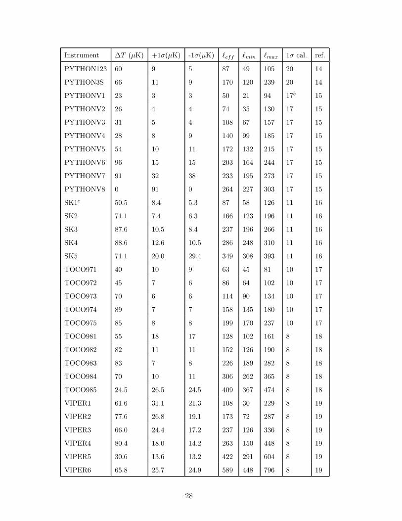
Table 1Complete compilation of CMB anisotropy observations 1992-1999, with maximumlikelihood ∆T , upper and lower 1σ uncertainties (not including calibration uncer-tainty), the weighted center of the window function, the ℓ values where the windowfunction falls to e−1/2 of its maximum value, the 1 σ calibration uncertainty, andreferences given below.
REFERENCES: 1–Tegmark & Hamilton (1997); Kogut et al. (1996a) 2–Ganga et al.(1994) 3–Gutierrez et al. (1999) 4–Femenia et al. (1998) 5–Ganga et al. (1997b);Gundersen et al. (1995) 6–Tucker et al. (1997) 7–Ratra et al. (1999) 8–Masi et al.(1996) 9–Dicker et al. (1999) 10–De Oliveira-Costa et al. (1998) 11–Clapp et al.(1994); Tanaka et al. (1996) 12–Ganga et al. (1998) 13–Wilson et al. (1999) 14–Platt et al. (1997) 15–Coble et al. (1999) 16–Netterfield et al. (1997) 17–Torbetet al. (1999) 18–Miller et al. (1999) 19–Peterson et al. (1999) 20–Mauskopf et al.(1999) 21–Scott et al. (1996) 22–Baker et al. (1999) 23–Leitch et al. (1998) 24–Ratraet al. (1998) 25–Ganga et al. (1997a); Church et al. (1997) 26–Partridge et al. (1997)27–Subrahmanyan et al. (1993) 28–Holzapfel et al. (1999) 29–Staren et al. (1999)aCould not be determined from the literature.bResults from combining the +15% and -12% calibration uncertainty with the 3µKbeamwidth uncertainty. The non-calibration errors on the PYTHONV datapointsare highly correlated.cThe SK ∆T and error bars have been re-calibrated according to the 5% increaserecommended by Mason et al. (1999) and the 2% decrease in ∆T due to foregroundcontamination found by De Oliveira-Costa et al. (1997).


![28. Cosmic Microwave Backgroundpdg.lbl.gov/.../rpp2019-rev-cosmic-microwave-background.pdf · 2019. 12. 6. · cosmic microwave background (CMB), discovered in 1965 [1]. The spectrum](https://static.documents.pub/doc/80x56/6143c67b6b2ee0265c02424a/28-cosmic-microwave-2019-12-6-cosmic-microwave-background-cmb-discovered.jpg)