The Cost of Capital for Alternative Investments

Jakub W. Jurek and Erik Stafford∗

Abstract

We develop a simple state-contingent framework for evaluating the cost of capital for non-linear

risk exposures, and show that properly computed required rates of return are meaningfully higher

than indicated by linear factor models. Given the large allocations of typical investors in alternatives,

many have not covered their cost of capital, despite earning an annualized excess return of 6.3%

between 1996 and 2010. A simple derivative-based strategy, which accurately matches the risk profile

of hedge funds, realizes an annualized excess return of 10.2% over this sample period, while providing

monthly liquidity and complete transparency over its state-contingent payoffs. Investable portfolios

based on popular factor models deliver annualized risk premia of 0-3% over the same period.

First draft: June 2011

This draft: November 2012

∗Jurek: Bendheim Center for Finance, Princeton University and NBER; jjurek@princeton.edu. Stafford: HarvardBusiness School; estafford@hbs.edu. We thank Joshua Coval, Ken French, Samuel Hanson, Campbell Harvey (editor),Jonathan Lewellen, Andrew Lo (discussant), Burton Malkiel, Robert Merton, Gideon Ozik (discussant), Andre Perold,Jeremy Stein, Marti Subrahmanyam (discussant), Russell Wermers (discussant), and seminar participants at DartmouthCollege, Harvard Business School, Imperial College, Bocconi University, USI Lugano, Princeton University, the 2012 NBERAsset Pricing Summer Institute, the 2011 NYU Five-Star Conference, the 4th NYSE Liffe Hedge Fund Research Conference,and the BYU Red Rock Finance Conference for helpful comments and discussions.

This paper develops a simple method for calculating the cost of capital for alternative investments.

Ex ante cost of capital estimates are central to the efficient allocation of capital, and generally depend on

the composition of the investor’s total portfolio and the payoff profile of the new investment relative to

the remainder of the portfolio. In the context of alternative investments, these allocations (1) constitute

a large share of the investor’s total portfolio and (2) have nonlinear payoffs relative to the remainder of

the portfolio at horizons that permit rebalancing. We find that these two features interact to produce

very large required rates of return relative to commonly used benchmarking techniques, including those

developed recently to address the nonlinear payoffs of alternative investments.

Merton (1987) develops a model of capital market equilibrium with incomplete information in which

investors must be informed about an investment before they allocate any capital to it. This creates

specialization in investing and leads some investors to hold highly concentrated portfolios in equilibrium.

As a result, the equilibrium required rate of the return on these investments exceeds what would be

required in a frictionless model. An important class of real world decisions to which this applies are

alternative investments. Conditional on investing in alternatives, allocations are typically large relative

to the equilibrium supply of these risks, in order to amortize the fixed costs associated with expanding

the traditional investment universe to include alternatives. For example, as of June 2010, the Ivy League

endowments had 40% of their combined assets allocated to non-traditional assets (Lerner, et al. (2008)),

whereas the share of alternatives in the global wealth portfolio was closer to 2%.1 This paper argues

that the wedge between the proper cost of capital and that implied by a frictionless model is likely to

be particularly large here due to the non-linearity of the payoff profile relative to the remainder of the

portfolio. Taking observed portfolio allocations as given, we study the role concentrated allocations

play in the cost of capital for alternative investments.

To the extent that the real world equilibrium is affected by market frictions that lead some investors

to hold highly concentrated portfolios, these consequences must be explicitly handled in cost of capital

estimates, but typically are not. For example, traditional cost of capital computations are heavily reliant

on linear factor models, which implicitly assume that: (a) investors trade in frictionless markets, and

thus hold efficient portfolios; and (b) asset returns are well described by the considered set of traded

factors. Merton (1987) highlights the theoretical and empirical challenges posed by the first assumption

when the equilibrium is one where a small subset of investors hold relatively large shares of a particular

1As of end of 2010, the total assets under management held by hedge funds stood at roughly $2 trillion (source: HFRI),in comparison to a combined global equity market capitalization of $57 trillion (source: World Federation of Exchanges) anda combined global bond market capitalization of $54 trillion, excluding the value of government bonds (source: TheCityUK,“Bond Markets 2011”).

1

risk, as appears to be the case for alternative investments. The linear factor model approach relies

on the notion that all agents agree on the required rate of return for a marginal deviation from their

efficient portfolios, but this will generally not be true when market frictions cause some investors to hold

concentrated portfolios. Ignoring this issue altogether, the focus of the empirical literature has been on

expanding the factor set (e.g. by adding non-linear factors) in an attempt to describe the downside risk

exposure of alternatives. Nonlinear factors have been included in an ad hoc way, such that they often

do not represent feasible investments, and are unlikely to capture the specific nonlinear risk profile of

hedge funds.2 We remedy these shortcomings, and produce cost of capital estimates for alternatives

reflecting the economic reality of the concentrated portfolio to which they belong.

To derive estimates of the cost of capital in a setting where investors make large allocations to

downside risks, we assemble a simple static portfolio selection framework that combines power utility

(CRRA) preferences, with a state-contingent asset payoff representation, in the spirit of Arrow (1964)

and Debreu (1959). We specify the joint structure of asset payoffs by describing each security’s payoff

as a function of the aggregate equity index (here, the S&P 500).3 Finally, to capture the non-linear

risk exposure of alternatives, we model hedge fund returns as a portfolio of cash and equity index

options. The contractual nature of index put options immediately provides a complete state-contingent

description of an investable alternative to the aggregate hedge fund universe. In turn, the availability of

a state-contingent risk profile allows us to determine the rate of return that an investor would require

as a function of his risk aversion, portfolio allocation, and the underlying return distributions of other

asset classes, all of which are necessary for any asset allocation decision.

Our first empirical contribution is to provide a new methodology for replicating the returns to a broad

cross-section of hedge fund indices. While evidence of non-linear systematic risk exposures resembling

those of index put writing has been provided by Mitchell and Pulvino (2001) for risk arbitrage, and

Agarwal and Naik (2004) for a large number of equity-oriented strategies, the literature – aside from

Lo (2001) – has been comparatively silent on exploring non-linear replicating strategies. We take

seriously the problem of capital requirements (Santa-Clara and Saretto (2009)) and transaction costs to

produce the returns of feasible put writing strategies, thus extending the linear hedge fund replication

2For example, Agarwal and Naik (2004) use options that are 1% out-of-the-money to explain hedge fund returns, whichmay not be the appropriate downside risk profile of these investments. Fung and Hsieh (2004) construct factors based onthe theoretical returns to lookback straddle portfolios, which represent highly infeasible portfolio returns since they do notsatisfy margin requirements.

3The same state-contingent payoff model is used in Coval, et al. (2009) to value tranches of collateralized debt obligationsrelative to equity index options, and in Jurek and Stafford (2012) to elucidate the time series and cross-section of repomarket spreads and haircuts.

2

analysis of Lo and Hasanhodzic (2007). For a given hedge fund index, we identify suitable replicating

strategies by matching the mean pre-fee returns of the index. Our procedure does not rely on linear

regression, and therefore sidesteps problems due to return smoothing or asset illiquidity (Asness, et al.

(2001), Getmansky, et al. (2004)). When compared with our put writing strategies, linear strategies

identified via in-sample regressions: (a) generate statistically significant shortfalls in replicating the

returns of hedge funds; (b) produce feasible residuals exhibiting greater skewness and excess kurtosis;

(c) do a inferior job of matching the drawdown patterns of hedge fund indices; and, (d) deliver minimal

improvements in explanatory R2, despite being designed to essentially maximize this statistic. To further

validate our replication methodology we examine the cross-section of HFRI subindices and compare the

fit of our put writing strategies against linear factor models out-of-sample, by selecting the replicating

strategies using the first half of the data (Jan. 1996 - Jun. 2003) and examining their performance

using the second half (Jul. 2003 - Dec. 2010). We find that for the set of equity-related hedge fund

subindices, where simple strategies based on equity index options can be expected to perform well, non-

linear replicating portfolios dominate their linear counterparts both along the dimension of matching

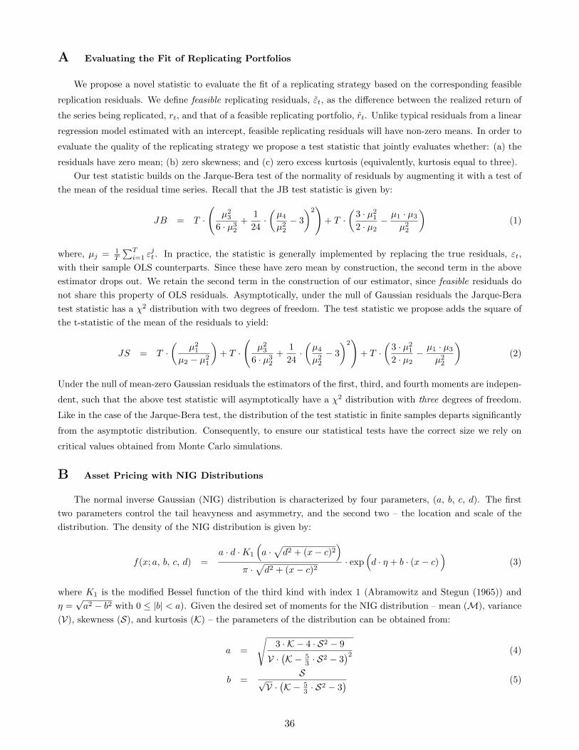
the risks, as well as, the returns. In the course of this analysis, we propose a novel test statistic for

evaluating the fit of a replicating strategy by measuring its ability to match the returns and higher-order

moments of the target return series. Our test statistic is a simple extension of the Jarque-Bera test for

the normality of the series, augmented by the squared value of the t-statistic for the mean of the series.

While the preceding analysis indicates that pre-fee hedge fund returns can be replicated using put

writing strategies, it has little to say about whether investors in either strategy have covered their proper

cost of capital. For example, to the extent that put options are fairly priced, our results indicate that

hedge funds may be earning compensation for jump and volatility risk premia. Another interpretation is

that put options are themselves mispriced, reflecting an imperfectly competitive market for the provision

of “pre-packaged” liquidity, such that a conclusion of zero after-fee alpha for hedge funds may still be

rejected.4 To confront this possibility directly, we use our state-contingent payoff framework combined

with the composition of the put writing strategies and the realized path of market volatility, to examine

the time series of the proper cost of capital for two types of investors in hedge funds. Both investors

hold 50% of their allocation to risky assets in alternatives; the first investor is assumed to hold risky

assets exclusively, while the second investor has a baseline allocation of 40% to risk-free securities and

4Option returns reflect the returns to bearing jump and volatility risk (e.g. Carr and Wu (2009), Todorov (2010)), aswell as, compensation for systematic demand imbalances (e.g. Garleanu, et al. (2009), Constantinides, et al. (2012)). Heand Krishnamurthy (2012) highlight the role of time-varying capital constraints of intermediaries on asset prices.

3

a 60% allocation to risky securities, mimicking the standard benchmark invoked by pension plans and

endowments.

Our second empirical contribution demonstrates that cost of capital computations based on ex post

factor regressions, or ex ante theoretical estimates based on the CAPM, meaningfully understate the

investors’ true cost of capital. For example, linear regressions (CAPM, Fama-French, Fung-Hsieh)

suggest that hedge fund investors have earned alphas ranging from 3-6% per annum net of fees. By

contrast, our model indicates that relative to the proper cost of capital – which accounts for the payoff

non-linearity of the aggregate hedge fund index and the concentrated investor allocations – the equity

investor earned an alpha of 1.0% (t-statistic: 0.5) and the endowment investor earned an alpha of -1.2%

(t-statistic: -0.6). The proper cost of capital for the endowment stands at 7.5% and is more than twice as

large as the theoretical prediction based on the CAPM beta of the aggregate hedge fund universe (3.1%),

and is even larger when compared to the cost of capital estimates based on the ex post factor regressions

commonly used in performance evaluation. We extend this analysis to the cross-section of equity-related

hedge fund strategies, and find that net of fees investor alphas are statistically indistinguishable from

zero for both investor types. In practice, many investors have likely underperformed their proper cost

of capital estimates as the hedge fund indices we study are likely to suffer from survivorship and backfill

bias (Malkiel and Saha (2005)), overstating the returns to actual hedge fund investors.

Finally, our state-contingent framework also allows us to provide a new perspective on the pricing

of equity index options. We find that the pre-fee put writing returns are consistently about 3.5% to

4% higher than their associated hedge fund strategy return, which translates into consistently positive

alphas for both investor types. The equity investor generally realized statistically significant alphas from

the put writing portfolios, while the endowment investor generally realized alphas that are statistically

indistinguishable from zero. While these finding qualitatively confirm that equity index puts are “ex-

pensive,” our estimates of annualized alphas are (at least) an order of magnitude lower than reported

in previous papers (e.g. Coval and Shumway (2001), Bakshi and Kapadia (2003), Bondarenko (2003),

Frazzini and Pedersen (2011), Constantinides, et al. (2012)). From the perspective of our model, the

marginal price setters in equity index options markets may simply hold portfolios that are even more

concentrated that the ones we considered, or believe the underlying equity index return distribution has

a more severe left tail than in our calibration.

The remainder of the paper is organized as follows. Section 1 describes the risk profile of hedge

funds. Section 2 presents a simple recipe for replicating the aggregate hedge fund risk exposure with

4

index put options and empirically compares the returns of this replication strategy with those produced

by linear factor models. Section 3 develops a generalized asset allocation framework for computing the

cost of capital for investors with large allocation to nonlinear payoffs. Section 4 evaluates the empirical

pricing of downside risks using after-fee hedge fund index returns, as well as, the pre-fee returns to put-

writing strategies, and compares them to inference based on traditional linear factor models. Finally,

Section 5 concludes the paper.

1 Describing the Risk Profile of Hedge Funds

We begin our investigation of hedge fund risk profiles with an assessment of the risk properties of

the aggregate asset class. We proxy the performance of the hedge fund universe using two indices: the

(value-weighted) Dow Jones/Credit Suisse Broad Hedge Fund Index, and the (equal-weighted) HFRI

Fund Weighted Composite Index. Such indices are not investable, and typically provide an upward

biased assessment of hedge fund performance due to the presence of backfill and survivorship bias. For

example, Malkiel and Saha (2005) report that the difference between the mean annual fund return in the

backfilled and non-backfilled TASS database was 7.34% per year in the 1994-2003 sample. Moreover,

once defunct funds are added in the computation of the mean annual returns to correct for survivorship

bias, the mean annual fund return declines by 4.42% (1996-2003). To the extent that the survivorship

bias also affects the measured risks, it is unlikely that the true risks are lower than those estimated

from the realized returns over this period. We discuss the implications of higher underlying risks and

how alternative economic outcomes are likely to affect alternative investments in Section 4.

Table 1 reports summary statistics for the HFRI and DJ/CS aggregates and their major sub-indices,

computed using quarterly returns from 1996:Q1-2010:Q4 (N = 60 quarters), and compares them to the

S&P 500 index and one-month T-bills. Although index returns are available at the monthly frequency,

we focus on quarterly returns throughout the paper to ameliorate the effects of stale prices and return

smoothing (Asness, et al. (2001), Getmansky, et al. (2004)). Finally, since our goal is to characterize

compensation for bearing risk across various markets rather than investor returns per se, we report

summary statistics for pre-fee index returns. To obtain pre-fee returns, we treat the observed net-of-

fee time series as if it represented the return of a representative fund that was at its high watermark

throughout the sample, and charged a 2% flat fee and a 10% incentive fee, both payable monthly.5 The

5In practice most funds impose a “2-and-20” compensation scheme, comprised of a 2% flat fee and a 20% incentiveallocation, subject to a high watermark provision. Our compensation scheme can therefore loosely be interpreted asdescribing the scenario where half of the funds in the universe are at their high watermark at each point in time. Our

5

difference between the mean pre-fee and net-of-fee returns represents an approximation of the all-in

investor fee. For comparison, using cross-sectional data from the TASS database for the period 1995-

2009, Ibbotson, et al. (2010) find that the average fund collected an all-in annual fee of 3.43%. French

(2008) reports an average total fee of 4.26% for U.S. equity-related hedge funds in the HFRI database

using data from 1996 through 2007. We find that our crude computation of all in-fees coincides well

with these estimates.

The attraction of hedge funds over this time period is clear: mean returns on alternatives exceeded

that of the S&P 500 index, while incurring lower volatility. Moreover, the estimated linear systematic

risk exposures (or CAPM β values) indicate that hedge fund performance was largely unrelated to

the performance of the public equity index, and suggests that relative to this risk model they have

outperformed. The realized pre-fee Sharpe ratios on alternatives were approximately three times higher

than that of the S&P 500 index. Under all of the standard risk metrics inspired by the mean-variance

portfolio selection criterion, hedge funds represented a highly attractive investment. Hedge funds also

perform well when evaluated on the dimension of drawdowns, which measure the magnitude of the

strategy loss relative to its highest historical value (or high watermark). Both hedge fund indices have

a minimum drawdown of approximately -20%, which is less than half of the -50% drawdown sustained

by investors in public equity markets. This is further illustrated in Figure 1, which plots the net-of-fee

value of $1 invested in the various assets through time. By December 2010, the hedge fund investor

had amassed a wealth roughly 50% larger than the wealth of the investor in public equity markets, and

more than twice the wealth of an investor rolling over investments in short-term T-bills.

The data also reveal the presence of significant non-normalities in hedge fund returns, as demon-

strated by the departures of the measured skewness and kurtosis from zero and three, respectively.

The Jarque-Bera (JB) statistic evaluates whether a time series exhibits skewness and kurtosis, and is

a popular test for normality. The 5% critical value for the JB test statistic in a sample of our size is

5.0, indicating that the null of normally-distributed returns is rejected for all, but four, of the eighteen

hedge fund sub-indices. This raises the possibility that the high measured CAPM alphas may not only

reflect manager skill, but also some compensation for exposure to (non-linear) downside risks.6

Figure 1 also confirms that the performance of hedge funds as an asset class is not market-neutral.

For example, hedge funds experience severe declines during extreme market events, such as the credit

computation is also likely conservative in that the incentive component represents an option on the pre-fee return of aportfolio of funds, rather than a portfolio of options on the pre-fee returns of the underlying funds.

6Harvey and Siddique (2000) provide an asset pricing model where skewness is priced, and present empirical evidenceof a systematic skewness risk premium in equity markets.

6

crisis during the fall of 2008 and the LTCM crisis in August 1998. During the two-year decline following

the bursting of the Internet bubble, hedge fund performance is flat. And, finally, in the “boom” years

hedge funds perform well. Empirically, the downside risk exposure of hedge funds as an asset class is

reminiscent of writing out-of-the-money put options on the aggregate index. Severe index declines cause

the option to expire in-the-money, generating losses that exceed the put premium. Mild market declines

are associated with losses comparable to the put premium, and therefore flat performance. Finally, in

rising markets the put option expires out-of-the-money, delivering a profit to the option-writer.

There are structural reasons to view the aggregated hedge fund exposure as being similar to short

index put option exposure. Many strategies explicitly bear risks that tend to realize when economic

conditions are poor and when the stock market is performing poorly. For example, Mitchell and Pulvino

(2001) document that the aggregate merger arbitrage strategy is like writing short-dated out-of-the

money index put options because the underlying probability of deal failure increases as the stock market

drops. Hedge fund strategies that are net long credit risk are effectively short long-dated put options

on firm assets – in the spirit of Merton’s (1974) structural credit risk model – such that their aggregate

exposure is similar to writing long-dated index put options. Other strategies (e.g. distressed investing,

leveraged buyouts) are essentially betting on business turnarounds at firms that have serious operating

or financial problems. In the aggregate these assets are likely to perform well when purchased cheaply

so long as market conditions do not get too bad. However, in a rapidly deteriorating economy these are

likely to be the first firms to fail.

The downside exposure of hedge funds is induced not only by the nature of the economic risks

they are bearing, but also by the features of the institutional environment in which they operate. In

particular, almost all of the above strategies make use of outside investor capital and financial leverage.

Following negative price shocks outside investors make additional capital more expensive, reducing the

arbitrageur’s financial slack, and increasing the fund’s exposure to further adverse shocks (Shleifer and

Vishny (1997)). Brunnermeier and Pedersen (2008) provide a complementary perspective highlighting

the fact that, in extreme circumstances, the withdrawal of funding liquidity (i.e. leverage) from to

arbitrageurs can interact with declines in market liquidity to produce severe asset price declines.

2 A New Method for Replicating Hedge Fund Risk Exposure

In order to replicate the aggregate risk exposure of hedge funds, we examine the returns to simple

strategies that write naked (unhedged) put options on the S&P 500 index. Our initial focus on replicating

7

the risk exposure of the aggregate hedge fund universe, rather than strategy sub-indices or individual

funds, is motivated by the observation that sophisticated investors (e.g. endowment and pension plans)

generally hold diversified portfolios of funds, either directly or via funds-of-funds. Consequently, a

characterization of the asset class risk exposure provides a first-order characterization of their problem.

We consider a range of replicating strategies with different downside risk exposures, as measured by

how far the put option is out-of-the-money and how much leverage is applied to the portfolio. Each

replicating strategy writes a single, short-dated put option, and is rebalanced monthly. Our hedge fund

replication methodology matches hedge fund indices to feasible put writing strategies on the basis of

their realized mean returns, and evaluates the model fit based on the distributional properties of the

feasible residuals, defined as the difference between the quarterly returns of the hedge fund index and the

feasible replicating portfolio. This approach takes seriously the notion that many hedge fund strategies

primarily bear downside risks resembling put writing, and that risk premia across economically similar

exposures should be equalized. To the extent that we incorrectly benchmark hedge fund performance

against an explicitly nonlinear strategy, we will produce residuals that have large skewness and kurtosis

relative to the residuals from linear factor models. On the other hand, to the extent that hedge fund

returns share the risk properties of put writing strategies, the put-writing-portfolio residuals will have

less skewness and kurtosis than those from linear factor model regressions.

Our proposed methodology, based on matching mean returns, contrasts starkly with existing ap-

proaches in the hedge fund replication literature, which fall into three broad categories: factor-based,

rule-based, and distributional. The factor-based methods, inspired by the ICAPM and APT, rely on

regression analysis to identify replicating portfolios of tradable indices, which in some cases include

option-based strategies (Fung and Hsieh (2002, 2004), Agarwal and Naik (2003, 2004), Lo and Hasan-

hodzic (2007)). A concern with the regression-based approach is that hedge fund return series are

smoothed (Asness, et al. (2001), Getmansky, et al. (2004)), which results in downward biased estimates

of factor loadings, and therefore upward biased estimates of hedge fund alphas. From a practical per-

spective, even after correcting for return smoothing by using lower frequency returns or adding lagged

factors, the portfolios of traditional risks identified by these regressions typically fail to match the high

excess returns delivered by hedge funds. The rule-based methods use mechanical algorithms to assemble

portfolios mimicking basic hedge fund strategies (Mitchell and Pulvino (2001), Duarte, et al. (2007)).

To the extent that hedge fund strategies bear risks distinct from those represented by commonly-used

asset pricing factors, an attractive feature of this approach is that the replicating portfolio will earn the

8

premia associated with those distinct risks by being directly exposed. For our purposes, a disadvantage

of this method is that the issue of determining the appropriate cost of capital for these risks remains

unresolved without a clear mapping into an asset pricing model. Finally, distributional methods focus

on matching the unconditional distribution of hedge fund returns, with no emphasis on matching con-

temporaneous movements between hedge funds and other assets, such as the market portfolio. This

approach is inspired by Dybvig’s (1988) payoff distributional pricing theory, which examines the prop-

erties of the cheapest-to-deliver lottery matching a given distribution, and was first applied to hedge

fund replication by Amin and Kat (2003). The general idea behind their approach is to identify a static

payoff function that transforms the distribution of the index return into the distribution of hedge fund

returns, and then replicate the static payoff through dynamic trading. While our approach shares the

flavor of using a transformation of the index return, through the choice of option strike and leverage

pairs, our model evaluation procedure explicitly relies on the contemporaneous replication residuals,

rather than the properties of the unconditional return distributions.

2.1 Measuring Put Writing Portfolio Returns

To calculate returns and characterize risks associated with put writing portfolios, we begin by spec-

ifying feasible investment strategies. Implementing each strategy requires defining the (1) rebalancing

frequency, (2) security selection rule, and (3) amount of financial leverage.

Each month from January 1996 through December 2010, we form a simple portfolio consisting of

a short position in a single S&P 500 index put option, P(K(Z), T ), and equity capital, κE(L), where

K(Z) is the option strike price, T is the option expiration date, and L is the leverage of the portfolio.

The portfolio buys (sells) put options at the ask (bid) prevailing at the market close of the month-end

trade date.7 If no market quotes are available for the option contract held by the agent at month-end,

the portfolio rebalancing is delayed until such quotes become available. The proceeds from shorting the

option, along with the portfolio’s equity capital are invested at the risk-free rate for one month, earning

rf,t+1. This produces a terminal accrued interest payment of:

AIt+1 =(κE(L) + Pbidt (K(Z), T )

)· (erf,t+1 − 1) . (1)

The monthly portfolio return, rp,t+1, is comprised of the change in the value of the put option plus the

7We aim to provide a conservative assessment of put writing returns by assuming the strategy demands immediacy byexecuting at the opposing side of the bid-ask spread. Returns measured on the basis of the option midprice are considerablyhigher given the wide bid-ask spread, especially in the early part of the sample.

9

accrued interest divided by the portfolio’s equity capital:

rp,t+1 =Pbidt (K(Z), T )− Paskt+1(K(Z), T ) + AIt+1

κE(L). (2)

We construct strategies that write options at fixed strike Z-scores. Selecting strikes on the basis of

their corresponding Z-scores ensures that the systematic risk exposure of the options at the rebalancing

dates is roughly constant, when measured using their Black-Scholes deltas. This contrasts with previous

studies, which have focused on strategies with fixed option moneyness (measured as the strike-to-spot

ratio, K/S, or strike-to-forward ratio), such as Glosten and Jagannathan (1994), Coval and Shumway

(2001), Bakshi and Kapadia (2003), Agarwal and Naik (2004). Options selected by fixing moneyness

have higher systematic risk, as measured by delta or market beta, when implied volatility is high, and

lower risk when implied volatility is low.

In particular, we define the option strike corresponding to a Z-score, Z, by:

K(Z) = St · exp(σt+1 · Z

)(3)

where St is the prevailing level of the S&P 500 index and σt+1 is the one-month stock index implied

volatility, observed at time t. We select the option whose strike is closest to, but below, the proposal

value (3), and whose expiration date is closest, but after the end of the month. At trade initiation,

the time to option expiration is roughly equal to seven weeks, since options expire on the third Friday

of the following month. To measure volatility at the one-month horizon, σt+1, we use the CBOE VIX

implied volatility index.

Option writing strategies require the posting of capital, or margin. The capital bears the risk of

losses due to changes in the mark-to-market value of the liability. The inclusion of margin requirements

plays an important role in determining the profitability of option writing strategies (Santa-Clara and

Saretto (2009)), and further distinguishes our approach from papers, where the option writer’s capital

contribution is assumed to be limited to the option price, as it would be for a long position. In the

case of put writing strategies, the maximum loss per option contract is given by the option’s strike

value, K. Consequently, a put writing strategy is fully-funded or unlevered (i.e. can guarantee the

terminal payoff) if and only if, the portfolio’s equity capital is equal to (or exceeds) the maximum loss

at expiration. For European options, this requires an initial investment of unlevered asset capital, κA,

10

equal to the discounted value of the exercise price less the proceeds of the option sale:

κA = e−rf,t+τ ·K(Z)− Pbidt (K(Z), T ) (4)

where rf,t+τ is the risk-free rate of interest corresponding to the time to option expiration, and is set on

the basis of the nearest available maturity in the OptionMetrics zero curves. The ratio of the unlevered

asset capital to the portfolio’s equity capital represents the portfolio leverage, L = κAκE

. Allowable

leverage magnitudes are controlled by broker and exchange limits, with values up to approximately

10 being consistent with existing CBOE regulations.8 We consider four put writing strategies, [Z,L],

all targeting an average realized return to match that of the hedge fund index being replicated. In

particular, we consider options at four strike levels, Z ∈ {−0.5,−1.0,−1.5,−2.0}, which are progressively

further out-of-the-money. The options we consider have strike prices that (at inception) are on average

between 4% (Z = -0.5) and 13% (Z = -2.0) below the prevailing strike price. By contrast, Agarwal and

Naik (2004), base their “out-of-the-money” put factor on options whose strike is 1% below the prevailing

spot price. Consequently, their approach is essentially equivalent to a linear regression methodology

which separately estimates the downside and upside betas, in the spirit of Glosten and Jagannathan

(1994). For each strike level, Z, we choose the leverage, L, such that the average strategy-level return

equals the mean realized return of the hedge fund strategy being considered over the estimation period.

2.1.1 An Example

To illustrate the portfolio construction mechanics consider the first portfolio rebalancing trade of

the [Z = −1, L = 2] strategy. The initial positions are established at the closing prices on January 31,

1996, and are held until the last business day of the following month (February 29, 1996), when the

portfolio is rebalanced. At the inception of the trade the closing level of the S&P 500 index was 636.02,

and the implied volatility index (VIX) was at 12.53%. Together these values pin down a proposal strike

price, K(Z) = 613.95, for the option to be written via (3). We then select an option maturing after the

next rebalance date, whose strike is closest from below to the proposal value, K(Z). In this case, the

selected option is the index put with a strike of 610 maturing on March 16, 1996. The [Z = −1, L = 2]

8The CBOE requires that writers of uncovered (i.e. unhedged) puts “deposit/maintain 100% of the option proceedsplus 15% of the aggregate contract value (current index level) minus the amount by which the option is out-of-the-money,if any, subject to a minimum of [...] option proceeds plus 10% of the aggregate exercise amount:

min κCBOEE = Pbid(K, S, T ; t) + max (0.10 ·K, 0.15 · S −max(0, S −K)) .

11

strategy writes the put, bringing in a premium of $2.3750, corresponding to the option’s bid price at the

market close. The required asset capital, κA, for that option is $603.56, and since the investor deploys

a leverage, L = 2, he posts capital of κE = $301.78. The investor’s capital is invested at the risk-free

rate, with the positions held until February 29, 1996. The risk-free rates corresponding to the trade

roll date (29 days) and maturity (45 days) are rf,t+1 = 5.50% and rf,t+τ = 5.43%, respectively, and are

obtained from the OptionMetrics zero-coupon yield curves. On the trade roll date, the option position

is closed by repurchasing the index put at the close-of-business ask price of $1.8750. This generates a

profit of $0.50 on the option and $1.3150 of accrued interest, representing a 60 basis point return on

investor capital. Finally, a new strike proposal value, which reflects the prevailing market parameters

is computed, and the entire procedure repeats.

2.1.2 Comparison to Capital Decimation Partners

Lo (2001) and Lo and Hasanhodzic (2007) examine the returns to bearing “tail risk” using a related,

naked put-writing strategy, employed by a fictitious fund called Capital Decimation Partners (CDP).

The strategy involves “shorting out-of-the-money S&P 500 put options on each monthly expiration

date for maturities less than or equal to three months, and with strikes approximately 7% out of the

money (Table 2, Panel A).” This strike selection is comparable to that of a Z = −1.0 strategy, which

between 1996-2010 wrote options that were on average about 7% out-of-the-money. By contrast, given

the margin rule applied in the CDP return computations, the leverage, L, at inception is roughly three

and a half times greater than our preferred hedge fund replication strategy. The CDP strategy is

assumed “to post 66% of the CBOE margin requirement as collateral,” where margin is set equal to

0.15 ·S−max(0, S−K)−P. In what follows, we interpret this conservatively to mean that the strategy

posts a collateral that is 66% in excess of the minimum exchange requirement. Abstracting from the

value of the put premium, which is significantly smaller than the other numbers in the computation,

and setting the risk-free interest rate to zero, the strategy leverage given our definition is:

LCDP =κAκE≈ 0.93 · S(

1 + 23

)· (0.15 · S −max(0, S − 0.93 · S))

= 6.975 (5)

This has led some to conclude that put-writing strategies do not represent a viable alternative to hedge

fund replication, due to difficulties with surviving exchange margin requirements. As we demonstrate,

this is not the case. The strategy that best matches the risk exposure of the aggregate hedge fund

universe is comfortably within exchange margin requirements at inception, and also does not violate

12

those requirements intra-month (unreported results).

2.2 Evaluating the Match for the Aggregate Index

To evaluate the quality of our replication procedure, we explore two sets of statistical tests. First, we

conduct linear regressions of hedge fund index returns onto standard asset pricing factors, and onto the

four put writing strategies identified by matching in-sample mean returns. By design, this procedure

minimizes the variance of the replication residuals without placing any feasibility constraints on the

strategies. For example, the factor regressions freely estimate the intercept even though any positive

estimate cannot be implemented by an agent seeking to replicate the returns of the index. In these

situations, the agent may replicate the risk of the index (i.e. achieve a high R2), while failing to replicate

the mean, which arguably motivates his interest in replication in the first place. Effectively, the focus of

these tests is on the second moment of the residuals. The second set of tests focuses on the distributional

properties of feasible replicating residuals, defined as the difference between the returns of the index and

a feasible replicating strategy (e.g. portfolio of tradable indices or a put-writing strategy). A credible

replication strategy should produce feasible residuals whose means are statistically indistinguishable

from zero (i.e. no shortfalls) and are roughly Gaussian, indicating the replicating strategy correctly

matches higher moments of the index. These tests complement the linear regressions by emphasizing

the feasibility of the replicating strategy and the identification of hedge fund index non-linearities, at

the expense of focusing on the variance of the residuals.

2.2.1 Linear Regressions vs. Matching on Means

The empirical literature studying the characteristics of hedge fund returns has focused on linear

regressions of index (and individual fund) returns onto replicating portfolios of tradable indices (Fung

and Hsieh (2002, 2004), Agarwal and Naik (2004), Lo and Hasanhodzic (2007)). Consequently, we are

interested in how the derivative-based risk benchmarks introduced in this paper compare with com-

monly used factor models in characterizing the realized returns of the aggregate hedge fund universe.

In particular, we consider several popular linear factor models, including the CAPM one-factor model;

the Fama-French/Carhart four-factor model; and the Fung-Hsieh nine-factor model, which was specif-

ically developed to describe the risks of well-diversified hedge fund portfolios (Fung and Hsieh (2001,

2004)). Five of the Fung-Hsieh factors are based on lookback straddle returns, to mimick trend-following

13

strategies, whose return characteristics are similar to being long options, or volatility (Merton (1981)).9

Table 2 reports results from regressions of hedge fund excess returns onto factor-mimicking portfolio

returns, alongside the corresponding regressions for the four mean-matched put writing portfolios. The

regressions use quarterly data spanning the period from January 1996 to December 2010. Table 2

indicates that relative to standard linear factor models (CAPM, Fama-French/Carhart, and Fung-

Hsieh) hedge funds have delivered pre-fee alphas between 7-10% per year, accounting for 67-97% of

the excess return earned by the aggregate hedge fund indices. Put differently, standard asset pricing

factors account for no more than a third of the risk premium earned by alternatives in the context of

the unconditional factor regression. Despite failing to match the mean return, the factor regressions

achieve explanatory R2 between 68% (CAPM) and 82% (Fama-French/Carhart). This highlights that

regression analysis minimizes the variance of the residuals without concern over the difference in mean

returns, as the intercept is a free parameter to absorb any shortfall (or surplus) in risk premium.

Of course, the feasible replicating strategy will not earn the return associated with the intercept.

Since our aim is to compare the linear replicating portfolios with our feasible put writing strategies,

we compute the returns to a feasible replicating portfolio based on the linear factor model regression

by including the intercept for estimation, but setting it to zero before computing fitted values. We

then compute feasible residuals for each linear factor model by subtracting the feasible fitted values

from the actual hedge fund returns. The resulting residuals represent the errors that an investor would

experience investing in a long-short portfolio consisting of the hedge fund index and the fitted replicating

benchmark. We calculate a feasible regression R2 by recomputing the standard R2 measure using feasible

residuals. This modification results in a notable decline in explanatory power, producing feasible R2

values ranging from 46% (Fung-Hsieh) to 69% (Fama-French/Carhart).

Since the put writing strategies are selected to match the mean in-sample return of the hedge fund

index, it is not surprising that the intercepts are statistically indistinguishable from zero, although this is

not entirely mechanical since the slope coefficient estimates depart from one. The put writing portfolios

have lower explanatory R2 when compared with the infeasible linear factor models that include the

intercept, but after applying the feasibility constraint, the put writing replicating portfolios deliver R2

values that are essentially in line with those of the linear models. For the put writing strategies, the

9To facilitate comparisons with the other factor models, we represent each of the factors in the form of equivalentzero-investment factor mimicking portfolios. Specifically, we make the following adjustments: (a) returns on the S&P 500and five trend following factors are computed in excess of the return on the 1-month T-bill (from Ken French’s website);(b) the bond market factor is computed as the difference between the monthly return of the 10-year Treasury bond return(CRSP, b10ret) and the return on the 1-month T-bill; and (c) the credit factor is computed as the difference between thetotal return on the Barclays (Lehman) US Credit Bond Index and the return on 10-year Treasury bond return.

14

feasible residuals are simply the difference in excess returns on the hedge fund index and those of the

mean-matched put writing strategies. The average feasible R2 of the three linear models is 55.3%, while

that of the non-linear models is 50.4%.

In another attempt to determine the quality of the match, we further project the hedge fund index

returns onto a constant and the returns of the various feasible replicating portfolios, and report the

p-values from the test of the null hypothesis that the intercept and slope are jointly equal to zero and

one, respectively. The only strategy not rejected at conventional significance levels using this test is the

[Z = −1, L = 2] put writing strategy; the rejections of the linear factor models owe to the presence of

statistically significant return shortfalls (intercepts), while those of the put writing replicating portfolios

owe to mismatches in riskiness (slopes).

2.2.2 Distributional Properties of Feasible Residuals

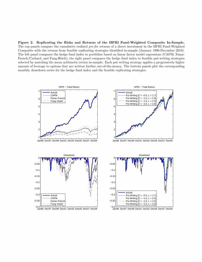
Figure 2 summarizes the statistical tests of Tables II and III by illustrating how the various distribu-

tional properties of the feasible residuals manifest themselves in the time series of accumulated investor

wealth. The two top panels display the value of an initial $1 investment in the hedge fund index and

each of the fitted linear factor model replicating portfolios (left panel) and each of the fitted put writing

replicating portfolios (right panel). The bottom panels plot the time series of drawdowns for each of

the replicating models. The linear factor models produce return series that look highly dissimilar to

the HFRI return series. On the other hand, all of the put writing strategies produce time series that

look virtually identical to the aggregate hedge fund index. The top left panel of Figure 2 shows how

the highly significant positive means in the feasible residuals from the linear factor models (Table II),

translate into large shortfalls in the terminal wealth levels, and that this feature is shared by all linear

models under consideration. By contrast, the put writing strategies match the losses during the fall of

2008 and the LTCM crisis, the flat performance during the bursting of the Internet bubble, as well as

the strong returns during boom periods. While the put writing strategy fails to explain some of the

return variation in economically benign times like the bull market between 2002 and 2007, it captures

the variation in economically important times remarkably well. This suggests that evaluating the ability

to replicate returns solely on R2 is missing some crucial properties of the overall fit.

In this section, we introduce a new test of the overall fit of a replicating strategy. Our motivation

follows from a causal decomposition of the time series properties of returns into: (1) benign variation; (2)

economically meaningful variation, characterized by large moves when a majority of risky investments

15

are moving in the same direction (i.e. large systematic drawdowns); and (3) the mean rate of return

(drift) over large intervals of time. Investors obviously care about mean returns, and in the presence of

return smoothing are also likely to emphasize the systematic exposure of a strategy in extreme economic

states over variation in benign environments. Given the presence of both skewness and excess kurtosis

in the raw hedge fund returns (Table 1), we evaluate the ability of the various replicating models to

produce zero-mean feasible residuals free of skewness and excess kurtosis. If we (incorrectly) benchmark

a strategy whose systematic exposure is linear against a non-linear put writing strategy, our tests will

reject the match. Similarly, strategies with non-linear exposures benchmarked against portfolios with

linear exposures will also be rejected.

Since we are interested in jointly characterizing the mean and non-normality of the feasible residuals,

a natural starting point for the design of a test statistic is the Jarque-Bera test. The Jarque-Bera

statistic (JB-statistic) tests whether a time series exhibits skewness and kurtosis, and is a popular

test for normality. We augment the Jarque-Bera tests statistic by combining it with the square of the

t-statistic for the mean of the of the feasible residuals. The new test statistic, which we refer to as the JS-

statistic, penalizes the feasible residuals for deviations from normality, as well as, large mean shortfalls

in replicating a desired returns series. The JS-statistic (JS = JB + (mean t-stat)2) is asymptotically

χ-square distributed with 3 degrees of freedom, since the JB-statistic has a χ-squared distribution with

two degrees of freedom, and the t-statistic of the mean is asymptotically Gaussian and independent of

the other two moment estimators. However, due to the well known deviations in the distribution of

the JB-statistic from its asymptotic distribution in finite samples, we base inference on finite-sample

distributions constructed by Monte Carlo.

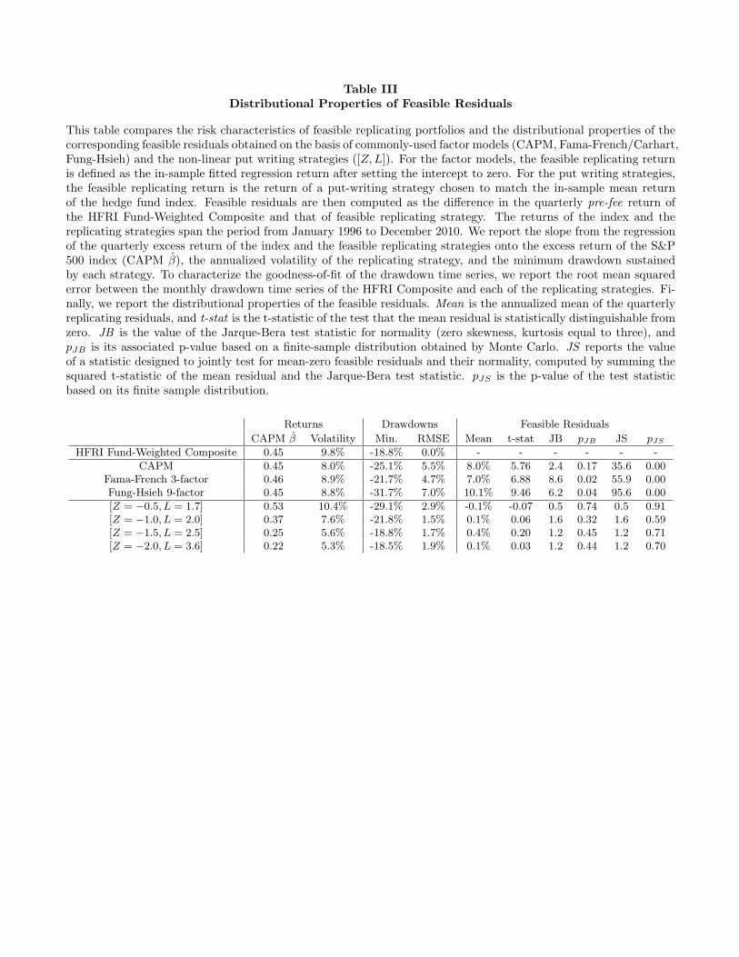
Table 3 summarizes the returns of the linear replicating portfolios and put-writing strategies, and

examines the properties of the corresponding feasible residuals. For each replicating strategy, the table

reports the estimated CAPM beta, annualized return volatility, the most severe drawdown, along with

the root mean squared error (RMSE) of the deviations between the drawdown time series of the hedge

fund index and those of the replicating strategy. In addition, we report an analysis of the distributional

properties of the quarterly feasible residuals using data from the full sample period from 1996 to 2010.

The replicating portfolios implied by the linear factor models all have CAPM betas of approximately

0.45, and annualized volatilities between 8-9%, which match the HFRI Composite well. The worst

drawdowns range from -22% to -32%, and generally exceed the maximum drawdowns experienced by

the aggregate index of -18.8%. The root mean squared errors of the deviations between the drawdown

16

time series of the index and the linear replicating strategies are economically large and range from 4.7%

to 7.0%. This confirms the intuition conveyed by the bottom left panel of Figure 2, which illustrates

that the drawdowns of the linear replicating strategies are poorly matched with those of the hedge fund

index. This owes in part to the failure of linear factor models to deliver enough drift to keep pace with

the index, thus slowing down the recovery following adverse shocks (e.g. the bursting of the Internet

bubble, the fall of 2008). The shortfalls between the linear factor model replicating portfolios and the

hedge fund index are measured by the mean of the feasible residuals. These are economically large

and highly statistically significant. The annualized shortfalls of the linear factor models range from

7-10% per annum with t-statistics ranging from 5.8 to 9.5. The feasible residuals exhibit some skewness

and kurtosis, though the Jarque-Bera statistic rejects normality only in the case of the CAPM. The

JS-statistic, which evaluates the model fit on the basis of normality and the ability to match mean

returns, strongly rejects all linear factor model replicating strategies.

By contrast, the put-writing strategies exhibit noticeable cross-sectional variation in their CAPM

betas, which decline monotonically from 0.53 for the [Z = −0.5, L = 1.7] strategy to 0.22 for the [Z =

−2.0, L = 3.6] strategy. Correspondingly, the volatilities and minimum drawdowns of the strategies also

decline. Intuitively, strategies applying higher leverage to further out-of-the-money options reallocate

losses to progressively worse states of nature, thus increasing their true economic risk. Linear CAPM

betas fail to capture this feature, instead suggesting a declining required rate of return. We return

to this point in Section 3, where we evaluate investors’ proper cost of capital for allocations to non-

linear risk exposures. When compared on the ability to match the time series of the hedge fund index

drawdowns, the Z = {−1,−1.5,−2} strategies are preferred to the Z = −0.5 strategy; all of the

non-linear replicating strategies strongly dominate their linear counterparts.

Since the non-linear put writing strategies were selected to match the in-sample mean of the hedge

fund index, the (annualized) mean of the feasible residuals is close to zero by construction. The JB-

statistics are uniformly smaller for the put writing models than for the linear models, although all

models do a good job of removing the skewness and excess kurtosis from the returns of the aggregate

hedge fund index. Due to the high-level of diversification in the aggregate hedge fund index it is not

as challenging a target in terms of non-normalities as the sub-strategy indices (Table 1). Finally, the

JS-statistic does not reject any of the put writing models.

To ensure the robustness of our results we have repeated our analysis using the Dow Jones/Credit

Suisse Broad Index, which is a value-weighted index designed to capture the performance of the aggregate

17

hedge fund universe. Given the similarities between the DJ/CS index and the HFRI index evident in

Figure 1, it is perhaps unsurprising that our results are qualitatively unchanged. Linear factor model

replicating portfolios fail to match the drift and drawdown patterns of this alternative hedge fund

index, unlike the put writing replicating portfolios. The four put-writing strategies selected in sample

are identical with the exception of the Z = −1.5 strategy, which applies a leverage of L = 2.6. Feasible

R2 values decline somewhat for both linear and non-linear models. All linear models continue to be

strongly rejected by the JS-test (p-values < 0.002); none of the put writing replicating portfolios are

rejected by the JS-test at the 1% level, and only the two most out-of-the-money portfolios are rejected

at the 5% level.

Finally, we verify that our results do not depend on our choice of working with pre-fee returns,

rather than the after-fee returns provided by HFRI and DJ/CS. To do this, we repeat the analysis

leaving the hedge fund index returns series unchanged, and instead searching over put writing strategies

which match the index returns after subtracting fees. To maintain consistency with our main analysis,

we apply a 2% flat fee to the put-writing returns and a 10% incentive fee, which is not subject to a high

watermark. Our results continue to hold for both indices. While the mean feasible residuals based on

the after-fee series are mechanically smaller – by roughly 4% per annum, reflecting our assessment of the

all-in fee paid by hedge fund investors – the JS-test continues to reject all linear replicating portfolios,

and none of the put-writing strategies.

2.3 Replicating Hedge Fund Strategy Returns Out-of-Sample

One interpretation of the results based on the analysis of the aggregate hedge fund indices is that

the put writing strategies capture a dimension of hedge fund risk that the linear factor models do not

capture and that this risk is associated with an economically large risk premium. For example, it is well

understood that option returns reflect the returns to bearing jump and volatility risk (e.g. Carr and Wu

(2009), Todorov (2010)), as well as, compensation for systematic demand imbalances (e.g. Garleanu, et

al. (2009), Constantinides, et al. (2012)). This is consistent with the notion that hedge funds specialize

in the bearing of a particular class of non-traditional, positive net supply risks, that may be highly

unappealing to a majority of investors. The close fit of the put writing replicating strategy indicates

that in spite of variation in the popularity of individual hedge fund strategies and institutional changes

in the industry, the underlying economic risk exposure of hedge funds in the aggregate has remained

essentially unchanged over the 15-year sample. At the individual strategy level, there are many reasons

18

to anticipate that risks change through time. The risk properties of the investable universe for a specific

strategy changes through time (e.g. the mix of cash-financed and stock-financed deals affects the overall

risk properties of merger arbitrage), views about appropriate leverage levels change over time, and the

actual classification of strategies is subject to modification through time.

Despite these potential challenges, we evaluate the performance of our replication methodology

out-of-sample using a cross-section of hedge fund sub-indices. Specifically, we use the first half of the

sample (Jan. 1996 - June 2003) to identify candidate replicating strategies for each hedge fund sub-

index; linear factor model replicating portfolios via in-sample regression and put-writing replicating

portfolios by matching mean in-sample returns. We then evaluate the quality of the match using the

second half of the data (July 2003 - December 2010). We split the full cross-section of twenty HFRI

and Dow Jones/Credit Suisse hedge fund indices reported in Table I into two groups: equity-related

and non-equity-related. The first group includes the aggregate indices studied earlier and strategies

that are likely to share the short-term downside exposure of the put writing portfolios (Event Driven,

Distressed, Merger Arbitrage, Equity Long/Short, Equity Market Neutral, and Equity Directional). The

second group includes strategies that trade primarily in intermediate or long-term credit, currencies,

and commodities (Relative Value, Convertible Arbitrage, Corporate, Macro and Managed Futures).

We report the results for the non-equity related strategies for completeness, though economic intuition

suggests that these are unlikely to be well described by the short-dated put writing strategies we focus

on in this paper. Many strategies in the non-equity grouping are exposed to interest rate risk, which

we do not model, unlike the Fung-Hsieh specification which includes two interest rate factors (term and

credit spread).10

The evaluation procedure involves producing out-of-sample returns and feasible residuals (differences

between the out-of-sample returns of each sub-index and the returns of the replicating strategies) for

each of the three linear factor models, and the four put-writing strategies. Since there are twenty hedge

fund indices and seven replicating portfolios we have a total of 140 out-of-sample time series of returns

and feasible residuals. To parsimoniously characterize our out-of-sample results for each index, we

collapse the time series of the replicating returns produced by the three linear models into a single time

series by weighting them according to the in-sample p-values of the JS-statistic. The intuition behind

this crude model averaging procedure is that we assign higher weight to models that do a better job of

10Coval, et al. (2009) and Jurek and Stafford (2012) show that long-dated credit exposures of structured and traditionalcorporate can be accurately described using portfolios of U.S. Treasuries and 5-year equity index options. Since thedynamics of long-dated volatility are generally distinct from those of short-dated volatility, the short-dated put-writingstrategies we explore are a priori not expected to capture interest rate or credit risk.

19

matching means and normalizing the residuals of the hedge fund index during the in-sample period. We

apply the same weighting scheme to the put writing replicating strategies. This produces two time series

of replicating returns per hedge fund index to be evaluated out-of-sample. Our results are qualitatively

unchanged if we simply select the strategy that provides the best in-sample fit within each model class,

and then use that model to construct out-of-sample replicating returns.

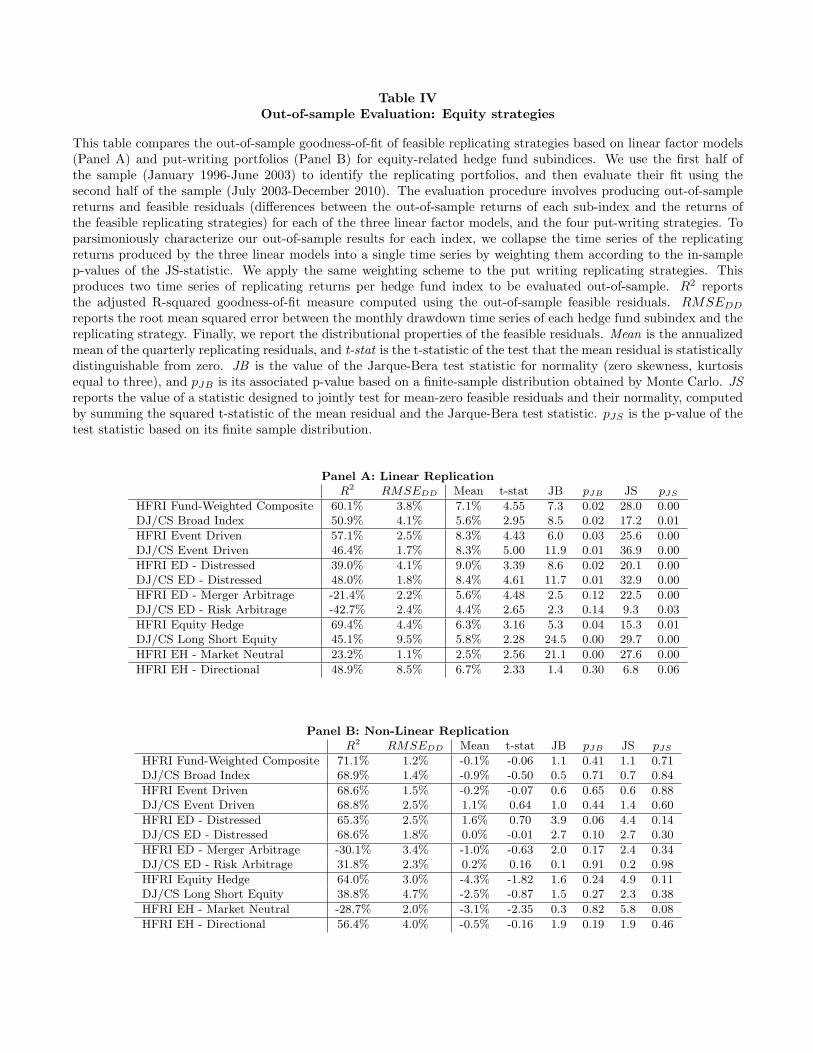
Tables IV and V report the results of this out-of-sample analysis. Panel A of each table reports the

fit of the linear replicating strategies, and Panel B summarizes the fit of the put writing strategies. Using

the out-of-sample returns, we report the feasible R2 to characterize the strategies’ ability to explain

monthly variation in returns, and the root mean squared error of the out-of-sample drawdown time

series to evaluate the downside risk exposure match. Finally, we examine the distributional properties

of the feasible residuals as in Table III.

Panel A shows that the linear replicating strategies fail to match the out-of-sample mean returns

of all twelve indices, as indicated by the presence of statistically significant mean residuals. The mean

shortfalls range from 2.5% (HFRI Equity Hedge: Market Neutral) to 9.0% (HFRI Event Driven: Dis-

tressed) and t-statistics between 2.3 and 5.0. Moreover, the linear replicating strategies produce highly

non-normal residuals, indicating they have failed to match the downside risk properties of the hedge

fund indices. The Jarque-Bera test rejects the normality of the the feasible residuals at the 5% level for

all but two investment styles. Taken together these facts combine to produce JS-statistics that strongly

reject the ability of linear models to replicate the returns and risks of all hedge fund styles, with the

exception of the HFRI Equity Hedge - Directional index.

Panel B reports the corresponding values for the out-of-sample fit of the put-writing strategies.

On average, the non-linear replicating strategies produce higher out-of-sample feasible R2 and match

the drawdown patterns of the hedge fund indices more closely. The put-writing strategies continue to

match the mean returns of the hedge fund strategies out-of-sample, producing mean feasible residuals

that are statistically significant in only one case (HFRI Equity Hedge - Market Neutral), where they are

negative, indicating that the put writing portfolio outperformed the corresponding hedge fund index.

The JB statistics are uniformly smaller for the put writing replicating portfolios than those of the linear

factor model replicating portfolios for each index individually. Normality of the feasible residuals is

not rejected at the 5% level for any hedge fund sub-index within this grouping. Correspondingly, the

JS-statistic never rejects the joint test that the put-writing strategy has matched the means returns

and risks of the hedge fund index at the 5% level.

20

Figure 3 summarizes these results and provides intuition for the JS-statistic by plotting the pairs of

(t-statistic of the mean feasible residual, JB-statistic) for each strategy/model class, along with the 5%

confidence level for each test statistic. The left panel corresponds to the in-sample estimation period

using the first half of the sample, while the right panel corresponds to the out-of-sample evaluation

period based on the second half of the sample. The out-of-sample plot shows that the put writing

model is never rejected on both dimensions across the twelve strategies considered, and only rejected

once for each the mean shortfall and the non-normality of feasible residuals. On the other hand, the

linear factor model is rejected on both dimensions for nine of the strategies considered, and for all of

the strategies in terms of mean shortfall in excess return.

Finally, Table V reports the out-of-sample fitting results for the non-equity-related hedge fund

subindices. The quality of the fit here is noticeably worse for both linear and non-linear replicating

portfolios as evidenced by the lower feasible R2 and higher root mean squared errors between the

drawdown time series of the actual index and the replicating strategies. The returns of the Macro and

Managed Futures categories are particularly poorly characterized. This is consistent with the summary

statistics reported in Table I, which indicate that the returns of these categories are largely unrelated

to the equity market index (low CAPM beta), and are in some instances, positively skewed. Across the

various sub-indices, the linear strategies continue to generate positive shortfalls, but their significance

is now diminished. Overall, the results from Table V suggest that the JS-test has power to reject the

put writing replicating strategies when the match is dissimilar and that even when there is little reason

to expect that the short-dated put writing portfolio represents a reasonable replicating strategy, it does

no worse than the linear factor model replicating strategies.

3 Required Rates of Return for Downside Risks

To study the investor’s cost of capital for alternative investments, we assemble a static framework,

which can accommodate the non-linear payoff profiles of the derivative replicating strategies introduced

in Section 2. The two fundamental ingredients of this framework are: (1) a specification of investor

preferences (utility); and, (2) a description of the joint payoff profiles (or return distributions) of the

assets under consideration. Using this framework we are able to characterize investor required rates of

return on traditional and non-traditional assets, as a function of portfolio composition, the structure of

the non-linear payoff representing the alternative, as well as, the risks of the market return distribution

(volatility, skewness, etc.). Our results illustrate that due to the payoff nonlinearity, the investor’s

21

proper cost of capital for alternatives (e.g. hedge funds) can deviate significantly from that implied

by linearized factor models, even when allocations are small. Furthermore, the nonlinearity interacts

strongly with the portfolio composition, producing a rapidly increasing cost of capital as a function of

the allocation to alternative investments.

3.1 The Investor’s Cost of Capital

Our static framework combines power utility (CRRA) preferences with a state-contingent asset

payoff representation originating in Arrow (1964) and Debreu (1959). Under power utility the investor

prefers more positive values for the odd moments of the terminal portfolio return distribution (mean,

skewness), and penalizes for large values of even moments (variance, kurtosis).11 To specify the joint

structure of asset payoffs, we describe each security’s payoff as a function of the log return, rm on the

aggregate equity index (here, the S&P 500).12 By specifying the joint distribution of returns using

state-contingent payoff functions, we can allow security-level exposures to depend on the market state

non-linearly, generalizing the linear correlation structure implicit in mean-variance analysis. Finally, to

operationalize the framework we need to specify the investor’s risk aversion, γ, and the distribution of

the log market index return, φ(rm).

We focus attention on a simple setting where the agent’s portfolio is comprised of an allocation to

cash, the equity index, and hedge funds. For every $1 invested, the state-contingent payoffs of the three

assets are as follows: the risk-free asset pays exp(rf · τ) in all states, the equity index payoff is, by

definition, exp(rm), and the payoff to the hedge fund investment is f(rm). The analysis in Section 2

indicates that the state-contingent payoff to alternatives can be accurately characterized using simple

levered portfolios of index put options justifying the existence of a suitable payoff representation, f(rm).

Given a realization of the market return, rm, the agent’s utility is given by:

U (rm | ωm, ωa) =1

1− γ·(

(1− ωm − ωa) · exp (rf · τ) + ωm · exp (rm) + ωa · f(rm))1−γ

(6)

where, ωm and ωa, are his allocations to the equity market and alternatives, respectively. Having

specified the investor’s utility function and a description of the asset payoff profiles – fundamental

11Patton (2004), Harvey, et al. (2010), and Martellini and Ziemann (2010) emphasize the importance of higher-ordermoments and the asset return dependence structure for portfolio selection.

12This applies trivially to index options, since their payoffs are already specified contractually as a function of the indexvalue. More generally, the framework requires deriving the mapping between a security’s payoff and the market statespace. Coval, et al. (2009) illustrate how this can be done for portfolios of corporate bonds, credit default swaps, andderivatives thereon.

22

ingredients of any portfolio choice framework – we can now either solve for optimal allocations by

maximizing his expected utility, taking asset prices as given; or solve for the investor’s required rate

of return on a new asset, as a function of his portfolio allocation, {ωm, ωa}, and the properties of the

equity index return distribution.

To compute the investor’s cost of capital for a risky asset, given a portfolio allocation {ωm, ωa}, it

will be useful to first define his subjective pricing kernel:

Λ (rm | ωm, ωa) = exp (−rf · τ) · U ′ (rm | ωm, ωa)E [U ′ (rm | ωm, ωa)]

(7)

The pricing kernel is random through its dependence on the realization of the (log) market return, rm,

and has been normalized, such that all agents agree on the pricing of the risk-free asset, independently

of their portfolio allocation and risk preferences. The shadow value of the alternative investment (or

any other payoff) is pinned down by the following individual Euler equation:

p∗a (ωm, ωa) = E [Λ (rm | ωm, ωa) · f (rm)] (8)

which corresponds to an annualized required rate of return of:

r∗a (ωm, ωa) =1

τ· log

E [f (rm)]

p∗a(9)

Under a special set of circumstances the investor’s required rate of return takes on a linear ex-

pected return-beta relationship (Ingersoll (1987), Cochrane (2005)). These generally require restrictive

assumptions regarding investors preferences (e.g. quadratic utility), return distributions (e.g. elliptical

distributions), and/or continuous trading. In general, none of these apply to the typical investor in

alternatives. First, given investors’ concerns about portfolio drawdowns, expected shortfalls, and other

(left) tail measures, it is clear that investor preferences are not of the mean-variance type. Second, there

is strong evidence of stochastic volatility and market crashes at the level of the aggregate stock market

index, such that the index returns not well described by the class of symmetric, elliptical distributions.

Since alternatives are non-linear transformations of index, the departures from symmetric distributions

become even more severe. Finally, investors in alternatives (e.g. pension plans, endowments) rebalance

their portfolios infrequently, and are typically subject to lockups. Despite these concerns, it is common

in the empirical literature to evaluate the performance of alternative investments using linear factor

23

models, frequently augmented with the returns to dynamic trading strategies (Section 2).

Given our focus on a single-factor payoff representation, we contrast the proper required rate of

return, (9), with the corresponding rate of return based on the linear CAPM rule, β · λ, where β =

Cov[ra, rm]V ar[rm] is the CAPM β of the alternative on the equity index and λ is the market risk premium. The

CAPM equilibrium logic identifies the market risk premium, λ, as the rate of return, under which the

representative investor is fully invested in the portfolio of risky assets. Given a risk aversion, γ, for the

representative agent, the equilibrium market risk premium is given by, λ = γ · σ2m.

3.2 Baseline Model Parameters

The investor’s cost of capital is a function of model parameters describing the distribution of the

(log) market return, investor’s risk tolerance, investor’s allocation to other assets, and the structure of

the alternative investment (e.g. option strike price and leverage). Before turning to a discussion of the

comparative statics of the investor’s cost of capital, we describe the baseline model parameters:

3.2.1 Investor types and risk aversion, γ

We consider two investor types in our analysis and calibrate the model, such that in the absence

of alternatives the first investor (γ = 2) would be fully invested in equities, while the second investor

(γ = 3.3) would hold a portfolio of 40% cash and 60% equities, corresponding to an allocation commonly

used as a benchmark by endowments and pension plans. Throughout our analysis, we refer to these

investors as the equity and endowment investors, respectively. In our empirical analysis, we assume

that the equity investor is fully invested in risky assets, and holds no cash. The endowment investor is

assumed to hold 80% of his portfolio in risky securities (equities + alternatives) and 20% of his portfolio

in cash. This allocation is typical of sophisticated endowments (Lerner, et al. (2008)), and represents

a tilt toward risky assets given the endowment investor’s risk aversion.

3.2.2 Equity index return distribution, φ(rm)

To illustrate the key features of the framework, we rely on the normal inverse Gaussian (NIG)

probability density to characterize the distribution of log equity index returns (Appendix A). We set

the annualized volatility, σ, of the distribution to 17.8%, or 0.8 times the average value of the CBOE

VIX index our sample (1996-2010: 22.2%). This scaling is designed to remove the effect of jump and

volatility risk premia embedded in index option prices used to compute the index (e.g. Carr and Wu

24

(2009), Todorov (2010)), as well as, the effect of demand imbalances (e.g. Garleanu, et al. (2009),

Constantinides, et al. (2012)).13 The remaining moments are chosen to roughly match historical

features of monthly S&P 500 Z-scores, obtained by demeaning the time-series of monthly log returns

and scaling them by 0.8 of the VIX as of the preceding month end. Specifically, we target a monthly

Z-score skewness, S, of -1, and kurtosis, K, of 7. These parameters combine to produce a left-tail

“event”once every 5 years that results in a mean monthly Z-score of -3.6. For comparison, the mean

value of the Z-score under the standard normal (Gaussian) distribution, conditional on being in the left

1/60 percent of the distribution, is -2.5.14 This pins down a conditional Z-score distribution from which

we simulate τ -period log index returns:

rm = (rf + λ− kZ(1)) · τ + Zτ , Zτ ∼ NIG (0, V, S, K) (10)

where V = σ2 · τ is the τ -period variance, and kZ(u) is a convexity adjustment term, given by the

cumulant generating function for the τ -period return innovation, Zτ :

kZ(u) =1

τ· lnE

[exp

(u · Zτ

)](11)

Appendix A shows that the equilibrium market risk premium, λ, equals:

λ = kZ (−γ) + kZ (1)− kZ (1− γ) (12)

Under the baseline model parameters, the Gaussian component of the equity risk premium equals 6.31%,

with the higher order cumulants contributing an additional 0.25%.15 Finally, we set the risk-free rate,

rf , and equity market dividend yield, δ, to their sample averages, which are equal to 3.1% and 1.7%,

13The scaling parameter was chosen on the basis of a historical regression of monthly realized S&P 500 volatility –computed using daily returns – onto the value of the VIX index as of the close of the preceding month (data: 1986:1-2010:10). The slope of this regression is 0.82, with a standard error of 0.05. Using the results and notation from AppendixA, the ratio of the historical, σP, to risk-neutral volatility, (σQ or VIX), is related to the NIG distribution parametersthrough:

σP

σQ =

(a2 − (b− γ)2

a2 − b2

) 34

At the baseline model parameters and a risk aversion of two, this ratio is equal to 0.92.14Based on a preceding month-end VIX value of 22.4%, and our parameterization of the NIG distribution, the -21.6%

return of the S&P 500 index in October 1987 corresponds to a Z-score of -4.7. The probability of observing a monthlyreturn at least as bad as this is 0.2% under the NIG distribution, and 0.0001% under the Gaussian distribution.

15The risk premium required by an investor with risk aversion γ, who holds exclusively the equity index is given by:

λ = γ · σ2 +1

τ·

(∞∑n=3

κnn!·(σ ·√τ)n · (1 + (−γ)n − (1− γ)n)

)

25

respectively.

3.2.3 Alternative investment, [Z, L]

The payoff of the alternative investment is represented using a levered, naked put writing portfolio,

as in the empirical analysis in Section 2. Specifically, we assume that the investor places his capital,

ωa, in a limited liability company (LLC) to eliminate the possibility of losing more than his initial

contribution. Limited liability structures are standard in essentially all alternative investments, private

equity and hedge funds alike, effectively converting their payoffs into put spreads. This has important

implications for the investor’s cost of capital, which we return to in the next section. Given a leverage

of L, the quantity of puts that can be supported per $1 of investor capital is given by:

q =L

exp (−rf · τ) ·K(Z)− P(K(Z), 1, τ)(13)

where K(Z) is the strike corresponding to a Z-score, Z. The put premium and the agent’s capital grow

at the risk free rate over the life of the trade, and are offset at maturity by any losses on the index puts

to produce a terminal state-contingent payoff:

f (rm) = max(

0, exp (rf · τ) · (1 + q · P(K(Z), 1, τ))− q ·max (K(Z)− exp (rm) , 0))

(14)

Using this payoff function, we also deduce that the limited liability legal structure corresponds to owning

q puts at the strike, K(LLC):

K(LLC) = K(Z)− exp (rf · τ) · 1 + q · P(K(Z), 1, τ)

q(15)

Finally, to compute the state-contingent payoff function of various put writing strategies, we also

need to supply market put values, P(K(Z), 1, τ). These determine the quantity of options sold,

and the LLC strike price. For the purposes of the comparative static analysis we assume a simple,

constant elasticity specification for the market (Black-Scholes) implied volatility function, σ(Z) =

σ(0) · exp(η · ln K(Z)

K(0)

). We set the at-the-money implied volatility, σ(0), equal to the sample aver-

age of the VIX index; the elasticity parameter, η, is set equal to -1.9, which is the mean OLS slope

coefficient from month-end regressions of implied volatilities onto log moneyness for options with ma-

where the κi are the cumulants of the distribution of the Z innovation. For a Gaussian distribution, all cumulants n > 2are equal to zero, and the equity risk premium is equal to γ · σ2.

26

turities corresponding to those studied in Section 2.

3.3 Comparative Statics

The comparative statics of the investor’s cost of capital computation are illustrated in Figure 4.

Each of the four panels plots the cost of capital in excess of the risk free rate as a function of share

of the investor’s risky portfolio allocated to alternatives. The left (right) panels represent the equity

(endowment) investor’s cost of capital for each of the four [Z,L] portfolios matching the mean returns of

the HFRI Fund Weighted Composite in-sample (1996:1-2003:6; Table III). The top panels correspond to

the scenario where the VIX index is at its full sample median (21.5%), and the bottom panels correspond

to the VIX being at its 90th percentile (31.5%).

The top left panel illustrates that from the risk tolerant (equity) investor’s perspective, the initial

allocation to alternatives commands a risk premium ranging from 2.9% to 4.3% per year depending on

which specific downside risk exposure is considered. The required rate of return increases steadily as

the share of the risky portfolio invested in alternatives rises, and particularly so, for the put writing

portfolios that apply high leverage to progressively further out-of-the-money options. Even at infinites-

imal allocations, investors reliant on CAPM cost of capital benchmarks will “observe” meaningful α’s,

even though a proper cost of capital would indicate the assets are priced correctly. For example, given

a beta of 0.45 (Table III) for the aggregate index, the required excess rate of return under the CAPM

rule would be roughly 2.7% (= 0.45 · 2 · (0.8 · 0.215)2). The wedge between the proper and linear risk

premia is a reflection of the linear model’s failure to properly risk adjust the payoff of the non-linear

put writing portfolios. This wedge increases further with the investor’s allocation, and is most severe

for the highly levered (i.e. more nonlinear) portfolios, which reallocate losses to states associated with

progressively worse economic outcomes. Since direct investors in hedge funds do not know the precise

features of their ultimate state-contingent payoff profiles, they must contemplate the possibility that

any of the four put writing portfolios identified in sample may represent the true risk profile, and weight

the corresponding required rates of return accordingly when allocating capital ex ante or evaluating

their performance ex post.

In practice, the fixed costs of investing in alternatives imply that the share of alternatives in investor

portfolios will not be infinitesimal (Merton (1987)). For example, Lerner, et al. (2008) document that

sophisticated endowments hold between 25% and 50% of their risky portfolio in alternatives.16 At a

16Lerner, et al. (2008) highlight a three-fold increase in alternative investment allocation at endowments over the periodfrom 1992-2005. For example, at the end of 2005 the median Ivy League endowment held 37% in alternatives, representing

27

50% share of the risky portfolio invested in alternatives, the risk tolerant investor would require a risk

premium between 5-6.5%. Equivalently, he would have to see an after fee annualized alpha between

2.2-3.8% relative to the linear CAPM rule simply to cover his properly computed required rate of return.

Strikingly, as allocations rise, the rank ordering of the required risk premia across the four non-linear

strategies cease to coincide with the rank ordering of their linear CAPM betas (Table III), suggesting

that ad hoc fixes to linear capital budgeting rules are unlikely to result in correct inference.

These deviations in required risk premia increase further for the more risk averse, endowment in-

vestors. Here the first dollar invested in alternatives must cover a required excess rate of return ranging

between 4.2% and 5.9%, depending on the specification of the non-linear payoff. These values exceed

the linear CAPM risk premia by 1.5-3.2% due to the tilt of the endowment investor’s portfolio towards

risky assets (20% allocation to cash vs. 40% equilibrium allocation), and the non-linearity of the payoff

profiles. The proper cost of capital is convex in the share of the risky portfolio in alternatives and at

a 50% portfolio share – characteristic of sophisticated University endowments – the proper risk pre-

mium is between 7.1-9.5%. These values are two to three times greater than the excess return required

under the CAPM rule, and indicate that managers reliant on linear risk models may be inefficiently

overallocating to alternatives.

The bottom two panels repeat the above analysis setting the level of the VIX index to its 90th

percentile over the 1996:1-2010:12 period, or 31.5%. Unsurprisingly, the investor required excess rates

of return increase sharply; recall that even under the CAPM the required excess rate of return is convex

in volatility. This effect is particularly strong for the non-linear payoff profiles. Not only does the level

of the required rate of return rise, but so does its sensitivity to the share of the risky portfolio allocated

to alternatives. This reflects the fact that the magnitude of the expected loss for the non-linear payoff

profiles increases with volatility, even though the strike-selection rule ensures the options are written

further out-of-the-money. This highlights that investors bearing the risk of alternatives in periods of

high volatility should properly require high risk premia. In a time series context, the strong convexity of

required rates of return in volatility indicates that the average required risk premium will be sensitive to

the volatility of the VIX, and will exceed the required rate of return computed at the sample average of

the VIX index. In unreported results, we also examine the sensitivity of investor required rates of return

to the tail risk of the underlying NIG distribution, as measured by the mean magnitude of the left-tail

Z-score observed once every five years. We find that required rates of return are likewise extremely

a 50% share of their risky asset portfolio (alternatives + equities). For the purposes of our risk analysis, we conservativelytreat fixed income investments as risk free.

28

sensitive to this metric, suggesting that our cost of capital computations are likely conservative if the

population density of the equity index return has a “worse” left tail than what has been observed in

the historical data.

4 Evaluating Downside Risks against a Proper Cost of Capital

Traditional cost of capital computations, based on linear factor models, assume that: (1) an investor’s

allocation to the risk being evaluated represents an infinitesimal deviation from their efficient portfolio,

and (2) the payoff structure of the risk can be well-described via its covariances with the factors. In

practice, neither of these assumptions fits the problem of a typical investor in alternatives. First, given

the specialized investment expertise required to evaluate and monitor these investments, it is common

for allocations to be large relative to the supply of these risks, in order to amortize the fixed costs

associated with expanding the investment universe to include alternatives (Merton (1987)). Second,

the analysis of feasible replicating residuals in Section 2 demonstrates that the returns of many hedge

fund strategies are matched more closely by the returns of (non-linear) put writing strategies, than by

the returns of replicating portfolios suggested by commonly used linear factor models (CAPM, Fama-

French, Fung-Hsieh). Taken together, these deviations suggest that inferences regarding the investor’s

cost of capital based on standard factor regressions are likely to be biased. Recall, such regressions

suggest a cost of capital ranging between 0-3% per annum (Table II). This section revisits the excess

returns to hedge fund strategies from the perspective of the state-contingent framework assembled in

Section 3, which was explicitly designed to handle large allocations to non-linear risks.

While the preceding analysis indicates that pre-fee hedge fund returns can be replicated using put

writing strategies, it has little to say about whether investors in either strategy have covered their proper

cost of capital. For example, to the extent that put options are fairly priced, this result indicates that

hedge funds are earning compensation for jump and volatility risk premia. Another interpretation is

that put options are themselves mispriced, reflecting an imperfectly competitive market for the provision

of “pre-packaged” liquidity, such that a conclusion of zero after-fee alpha for hedge funds may still be

rejected. To confront this possibility directly, we use our framework to jointly compare the returns of

put writing strategies and net-of-fee returns to hedge fund investments against the cost of capital based

on the framework proposed in Section 3.

29

4.1 The Time Series of the Proper Cost of Capital

To evaluate the realized performance of the aggregate hedge fund universe and the equity-related

sub-indices that were well-described by the put writing portfolios, we use the state-contingent payoff

model developed in Section 3 to produce a time series of required rates of return for the two investor

types introduced in the previous section. The relatively risk tolerant equity investor has a risk aversion

that permits him to be fully invested in stocks, but we assume he splits his allocation to risky assets

evenly between stocks and the alternative. The endowment investor would normally allocate 60% to

stocks and 40% to risk-free securities, but we assume they allocate 40% to stocks, 40% to alternatives,

and 20% to risk-free securities, to match the typical holdings of the Ivy League endowments.

To produce the time series of proper required rates of return for each investor type and each con-

sidered downside risk profile, at each rebalancing date we supply the model the specific composition of

the fitted put writing replicating portfolio for various hedge fund indices considered in Section 2, along

with parameters characterizing the terminal distribution of the (log) equity index return. At each point

in time, the composition of the put writing replicating portfolio is pinned down by the option strike,

K(Z), and the option price, P(Z), which jointly with L, determine the quantity of options sold, and

the investor’s capital. For parsimony, we hold the skewness and kurtosis of the market return distri-

bution fixed at their baseline values, and only let the market return volatility, σt, vary through time,

by setting it equal to 0.8 times the prevailing value of the VIX on each rebalancing date. The time

series of market volatility also pins down the time series of the equilibrium market risk premium, λt, via

(12). For comparison, we also produce a time series of required rates of return for hedge funds based on

the linear CAPM model by multiplying the βt of the option replicating portfolio (at inception) by the

CAPM market risk premium, γ · σ2t , where γ is the risk aversion of the all equity (marginal) investor.

Before comparing the model required rates of return to the realized returns of hedge funds and

put writing strategies, we convert the marginal, continuously compounded required rates of return,

r∗a(ωm, ωa), given by (9) and plotted in Figure 4, into discretely-compounded net returns, and compute

an average required rate of return given the investor’s allocation to alternatives, ωa. To obtain the

discretely compounded monthly return, we scale the annualized continuously compounded rate by 112 ,

exponentiate it, and subtract one. Then for each investor type, we average their marginal rates over a

fine grid of allocations to alternatives starting at zero and ending at ωa. We repeat this procedure at

each rebalancing date to produce a monthly time series of average required rates of return for use in

performance evaluation.

30

Finally, we note that over the sample period from 1996 through 2010, the stock market index

realized, on average, an annualized excess return of 5.1%, while the equity investor with no allocation to

alternatives required 7.6% per year, given the realized path of volatility over the sample. The endowment

investor with no allocation to alternatives, but with the “risk-on” tilt towards stocks, required 10.4%

per year. These estimates reflect the severe consequences of 2008 and 2009, when realized returns were

low and realized volatility was high. Over the more economically benign period of 1996 through 2007,

the stock market index average annual excess return is 6.5%, the required excess return for the equity

investor is 6.2% and that for the endowment investor is 8.4%. These computations suggest that our

model calibration produces sensible required rates of return for traditional investments.

4.2 Estimates of Hedge Fund Alphas

Panel A of Table 6 reports the annual time series of mean annualized excess rate of return (after-fees)

realized by the HFRI Composite Index and the (pre-fee) put-writing replicating portfolio, as well as the

mean annualized required excess rates of return for both investor types. Mean reports the full-sample

average of the annualized excess rates of return, with t-statistics reported in square brackets. The

mean required excess rate of return under the model is 5.3% for the equity investor and 7.5% for the

endowment investor. Both of these quantities are significantly higher than the CAPM required excess

rate of return, which stands at 3.1%. The wedge between the model and linear CAPM risk premia

reflects the non-linearity of the downside risk exposure, as well as the concentrated portfolio allocations

of the two investors. The model risk premium is very volatile, averaging nearly 20% for the endowment

investor in 2008 and 2009, when both the VIX and realized volatility are high. Panel B reports estimated

alphas based on the CAPM and the generalized model required rate of return for both investor types for

the HFRI Fund Weighted Composite. The annualized CAPM alpha is 3.2% (t-statistic = 1.6), which

is nearly 1% lower than the one reported in Table 1 due to the average of the time varying CAPM risk

premium being somewhat higher than the market risk premium realized in-sample. Specifically, the

realized market excess return in sample was 5.4% per annum versus a theoretical CAPM market equity

risk premium of 7.2% per annum. The equity investor realizes an annualized alpha of 1.0% (t-statistic =

0.5), while the endowment investor realizes an annualized alpha of -1.2% (t-statistic = -0.6), neither of

which are statistically distinguishable from zero. These results indicate that sophisticated endowment

investors, who had access to performance comparable to that of the survivorship-biased index, have

barely covered their properly computed cost of capital.

31

Table 6 also reports the results from these same analyses conducted on the pre-fee put writing

replicating portfolio, which was found to match well the risk properties of the HFRI index, and therefore

commands the same required return. The mean annualized excess return of the put writing portfolio

exceeds that of the after-fee HFRI index by 4% per year, indicating that a passive low cost exposure

to downside risk through index derivatives may be preferable to direct investment in hedge funds. For

example, the equity investor earns an alpha of 5% (t-statistic: 2.6) per year, and the endowment investor

earns an alpha of 2.7% (t-statistic: 1.4) per year. This suggests that the put-writing strategy offers an

attractive risk-adjusted rate of return relative to our model, even when it comprises 50% of the risky

portfolio share. We investigate this in more detail below.

Table 7 reports alpha estimates for the equity-related HFRI sub-indices whose risks were generally

well-explained by the put writing replicating portfolios. As before, we compute alpha estimates relative

to the linear CAPM model, and the generalized model for the equity and endowment investors. Panel

A displays results for the after-fee hedge fund indices and Panel B displays those for the associated

pre-fee put writing portfolios. The equity investor realized consistently small positive, but statistically

unreliable alphas across all of the considered strategies over the period 1996-2010, while the endowment

investor realized consistently negative, and again, statistically unreliable alphas. Only one of the t-

statistics across the 24 reported for the generalized model in Panel A exceeds 1.0 in magnitude. This

suggests that the investors in equity-related hedge funds have essentially earned their cost of capital.

Overall, the evidence presented in Tables 6 and 7 is inconsistent with claims that sophisticated

endowment investors earned an “illiquidity premium” for investing in alternatives. To the extent that

such a risk premium is in fact responsible for explaining the realized returns on the HFRI Composite

and the put writing strategy, this channel has been left unmodelled in our cost of capital computations.

Consequently, our cost of capital estimates are biased downward. Even relative to this impoverished

benchmark, we find that investors with concentrated hedge fund allocations did not earn statistically

reliable alphas after fees between 1996 and 2010. This casts doubt on the so-called “endowment model”

which is based on the premise that illiquid investments earn an additional risk premium that long-term

institutional investors will have a comparative advantage in bearing (Swensen (2000)). Finally, while it

is reasonable to expect that the first endowments to allocate to alternatives have actually earned the

returns associated with the published indices, thus covering their cost of capital, more recent investors

in alternatives are likely to have earned something closer to the average fund-of-fund return. These

returns are on average over 300 basis points lower per year, than the reported average aggregate hedge

32

fund return, suggesting these investors have not covered their cost of capital.

4.3 A New Perspective on the Expensiveness of Index Put Options

The pre-fee put writing returns are consistently about 3.5% to 4% higher than their associated hedge

fund strategy return, which translates into consistently positive alphas for both investor types. The

equity investor generally realized statistically significant alphas from the put writing portfolios, while

the endowment investor generally realized alphas that are statistically indistinguishable from zero.

These findings contrast with much of the existing literature, which documents high negative (positive)

risk-adjusted returns to buying (selling) index options (e.g. Coval and Shumway (2001), Bakshi and

Kapadia (2003), Bondarenko (2003), Frazzini and Pedersen (2011), Constantinides, et al. (2012)).17

The conclusion of index put options being highly expensive implicitly assumes that an investor who is

short these portfolios would earn the negative of the long portfolio returns. This is far from the reality,

as an investor with a short position would be required to post sufficient margin to initiate the position

and maintain sufficient margin to survive the sample paths realized ex post in the data (Santa-Clara

and Saretto (2009)).

The annualized alphas we report are an order of magnitude lower than reported in previous papers.

This difference is due to: (1) incorporating margin requirements, as emphasized by Santa-Clara and

Saretto (2009); and (2) a cost of capital computation that explicitly accounts for the non-linearity of the

payoff profiles and investor portfolio concentration. Importantly, the large margin requirements for short

positions in index put options effectively make these positive net supply assets; the supplier of these

payoffs has to allocate considerably more capital to this activity than that implied in the frictionless

models of Black-Scholes/Merton (1973). Moreover, this is a risk that is not well distributed throughout

the economy, as the suppliers of these securities are typically highly specialized in bearing this risk. The

same channel highlighted in our paper – concentrated portfolios require additional risk premium above

the frictionless model, especially when a nonlinear downside exposure is present – manifests itself here.

From the perspective of the frictionless model, both alternative investments and index put options seem

expensive, but much less so from the perspective of specialized investors (see also, Garleanu, Pedersen,

and Poteshman (2009)). These two frictionless model anomalies are fairly consistent with one another

after accounting for these two notable features.

17Coval and Shumway (2001) report that zero-beta, at-the-money straddle positions produce average losses of approx-imately 3% per week. Bakshi and Kapadia (2003) conclude in favor of a negative volatility risk premium by examiningdelta-hedged options returns. Frazzini and Pedersen (2011) report mean monthly delta-hedged excess returns between-9.5% (at-the-money) and -30% (deep out-of-the-money) for one-month index put options.

33

Finally, from the perspective of our model, the marginal price setters in equity index options markets

may simply hold portfolios that are even more concentrated that the ones we considered. Moreover, it

is important to recall that these calculations rely upon a specific distributional assumption about the

underlying stock market index, which is roughly consistent with the historical experience. A slightly

worse left tail will have a meaningful effect on the required returns for these portfolios, given their

nonlinear risk profiles and the large allocation sizes.

5 Conclusion

This paper argues that the risks borne by hedge fund investors are likely to be positive net sup-

ply risks that are unappealing to average investors, such that they may earn a premium relative to

traditional assets. A distinguishing feature of many of these risks is that their payoff profiles have a

distinct possibility of being non-linear with respect to a broad portfolio of traditional assets. These

non-linearities can arise either directly from the underlying economic risk exposure (e.g. credit risk,

merger arbitrage), or through the institutional structure through which they are borne (e.g. funding

liquidity). Our analysis focuses attention on investors with potentially large allocation to such non-

linear risk exposures, who may only be allowed to rebalance infrequently. This setup is common in

practice, but infrequently examined in the literature, which has placed emphasis on continuous trading

and/or assets whose risks can be well described by their covariance with each other over the rebalancing

horizon.

We begin by documenting that simple put writing strategies can be used to match both the risks and

pre-fee returns of the aggregate hedge fund universe, as well as, many equity-related hedge fund sub-

indices. This contrasts starkly with replicating strategies suggested by linear factor models (CAPM,

Fama-French/Carhart, Fung-Hsieh), which deliver high R2, but consistently fail to match the mean

rate of return of a hedge fund indices. Our non-linear replicating strategies dominate linear replicating

portfolio both in-sample and out-of-sample. Along the way, we introduce a novel test statistic, which can

be used to evaluate the ability of a feasible replicating strategy to match the returns and higher-order

moments of the target return series.

We then exploit the transparency of the state-contingent payoffs of the risk-matched put writing

portfolios to develop estimates of the cost of capital for allocations to alternatives with downside risks.

The model required rates of return vary as a function of investor preferences and allocations, the non-

linearity of the portfolio (option strike price and leverage), and the properties of the underlying equity

34

market return distribution (volatility and tail risks). One of the attractive features of this simple

generalized framework is that it conceptually requires no information beyond the traditional analysis,

although in practice it will require more sophisticated judgment over the state-contingent risk profile of

alternative investments.

An accurate assessment of the cost of capital is fundamental to the efficient allocation of capital

throughout the economy. Investment managers should select risks that are expected to deliver returns

at least as large as those required by their capital providers. The investors in alternatives should

require returns for each investment that compensate them for the marginal contribution of risk to

their overall portfolio. In the case of investments with downside exposure, the magnitude of these

required returns is large relative to those implied by linear risk models. As the allocation to downside

risks gets large, the marginal contribution of risk to the overall portfolio expands quickly, requiring

further compensation. In practice, investors frequently seem surprised by increases in return correlations

between alternatives and traditional assets (or between alternatives themselves) as economic conditions

deteriorate, suggesting they may not fully appreciate their portfolio-level downside risk exposure. This

ex post surprise likely coincides with meaningful ex ante errors in estimates of required rates of return,

and therefore inappropriate capital allocations. The calibrations in this paper suggest that despite the

seemingly appealing return history of alternative investments, many investors have not covered their

cost of capital.

35

A Evaluating the Fit of Replicating Portfolios

We propose a novel statistic to evaluate the fit of a replicating strategy based on the corresponding feasible

replication residuals. We define feasible replicating residuals, εt, as the difference between the realized return of

the series being replicated, rt, and that of a feasible replicating portfolio, rt. Unlike typical residuals from a linear

regression model estimated with an intercept, feasible replicating residuals will have non-zero means. In order to

evaluate the quality of the replicating strategy we propose a test statistic that jointly evaluates whether: (a) the

residuals have zero mean; (b) zero skewness; and (c) zero excess kurtosis (equivalently, kurtosis equal to three).

Our test statistic builds on the Jarque-Bera test of the normality of residuals by augmenting it with a test of

the mean of the residual time series. Recall that the JB test statistic is given by:

JB = T ·

(µ2

3

6 · µ32

+1

24·(µ4

µ22

− 3

)2)

+ T ·(

3 · µ21

2 · µ2− µ1 · µ3

µ22

)(1)

where, µj = 1T

∑Ti=1 ε

jt . In practice, the statistic is generally implemented by replacing the true residuals, εt,

with their sample OLS counterparts. Since these have zero mean by construction, the second term in the above

estimator drops out. We retain the second term in the construction of our estimator, since feasible residuals do

not share this property of OLS residuals. Asymptotically, under the null of Gaussian residuals the Jarque-Bera

test statistic has a χ2 distribution with two degrees of freedom. The test statistic we propose adds the square of

the t-statistic of the mean of the residuals to yield:

JS = T ·(

µ21

µ2 − µ21

)+ T ·

(µ2

3

6 · µ32

+1

24·(µ4

µ22

− 3

)2)

+ T ·(

3 · µ21

2 · µ2− µ1 · µ3

µ22

)(2)

Under the null of mean-zero Gaussian residuals the estimators of the first, third, and fourth moments are indepen-

dent, such that the above test statistic will asymptotically have a χ2 distribution with three degrees of freedom.

Like in the case of the Jarque-Bera test, the distribution of the test statistic in finite samples departs significantly

from the asymptotic distribution. Consequently, to ensure our statistical tests have the correct size we rely on

critical values obtained from Monte Carlo simulations.

B Asset Pricing with NIG Distributions

The normal inverse Gaussian (NIG) distribution is characterized by four parameters, (a, b, c, d). The first

two parameters control the tail heavyness and asymmetry, and the second two – the location and scale of the

distribution. The density of the NIG distribution is given by:

f(x; a, b, c, d) =a · d ·K1

(a ·√d2 + (x− c)2

)π ·√d2 + (x− c)2

· exp(d · η + b · (x− c)

)(3)

where K1 is the modified Bessel function of the third kind with index 1 (Abramowitz and Stegun (1965)) and

η =√a2 − b2 with 0 ≤ |b| < a). Given the desired set of moments for the NIG distribution – mean (M), variance

(V), skewness (S), and kurtosis (K) – the parameters of the distribution can be obtained from:

a =

√3 · K − 4 · S2 − 9

V ·(K − 5

3 · S2 − 3)2 (4)

b =S√

V ·(K − 5

3 · S2 − 3) (5)

36

c = M− 3 · S ·√V

3 · K − 4 · S2 − 9(6)

d =3

32 ·√V ·(K − 5

3 · S2 − 3)

3 · K − 4 · S2 − 9(7)

In order for the distribution to be well-defined we need, K > 3 + 53 · S

2. The NIG-distribution has closed-form

expressions for its moment-generating and characteristic functions, which are convenient for deriving equilibrium

risk premia and option prices. Specifically, the moment generating function is:

E [exp(u · x)] = exp

(c · u+ d ·

(η −

√a2 − (b+ u)

2

))(8)

B.1 Pricing Kernel and Risk Premia

Suppose the value of the aggregate wealth portfolio evolves according to:

Wt+τ = Wt · exp(

(µ− kZ (1)) · τ + Zt+τ

)(9)

where kZ(u) the cumulant generating function of random variable Zt+τ :

kZ(u) =1

τ· lnEt [exp (u · Zt+τ )] = c · u+ d ·

(η −

√a2 − (b+ u)2

)(10)

If markets are complete, there will exist a unique pricing kernel, Λt+τ , which prices the wealth portfolio, as well as,

the risk-free asset. Assuming the representative agent has CRRA utility with coefficient of relative risk aversion,

γ, the pricing kernel in the economy is an exponential martingale given by:

Λt+τΛt

= exp(− rf · τ − γ · Zt+τ − kZ (−γ) · τ

)(11)

Now consider assets whose terminal payoff has a linear loading, β, on the aggregate shock , Zt+τ , and an

independent idiosyncratic shock, Zi,t+τ :

Pt+τ = Pt · exp(

(µ(β)− kZ(β)− kZi(1)) · τ + β · Zt+τ + Zi,t+τ

)(12)

where µ(β) is the equilibrium rate of return on the asset, and the two k(·) terms compensate for the convexity

of the systematic and idiosyncratic innovations. For example, when β = 1 and the variance of the idiosyncratic

shocks goes to zero, the asset converges to a claim on the aggregate wealth portfolio. Assets with β < 1 (β > 1)

are concave (convex) with respect to the aggregate wealth portfolio.

To derive the equilibrium risk premium for such assets, we make use of the equilibrium pricing condition:

Λt · Pt = Et [Λt+τ · Pt+τ ] ⇔ 0 =1

τ· lnEt

[Λt+τΛt· Pt+τPt

](13)

Substituting the payoff function into the above condition and taking advantage of the independence of the aggre-

gate and idiosyncratic shocks, yields the following expression for the equilibrium risk premium on an asset with

loading β on the aggregate wealth shock:

µ(β)− rf = kZ (−γ) + kZ (β)− kZ (β − γ) (14)

37

This expression generalizes the standard CAPM risk-premium expression from mean-variance analysis to allow

for the existence of higher moments in the shocks to the aggregate market portfolio. For a Gaussian-distributed

shock, Zt+τ , the cumulant generating function is given by kZ(u) = 1τ ·

(σ·√τ ·u)

2

2 , such that, (14), specializes to:

µ(β)− rf =σ2

2·((−γ)2 + β2 − (β − γ)2

)= β · γ · σ2 = β · (µ(1)− rf ) (15)

In our generalized setting, the risk premium on an asset with loading β on the innovations to the market portfolio

does not equal β times the market risk premium, unlike in the standard CAPM. The discrepancy is specifically

related to the existence of higher moments in the shocks to the aggregate market portfolio.

Equilibrium risk premia can also be linked to the moments of the underlying distribution of the shocks to the

aggregate portfolio, by taking advantage of an infinite series expansion of the cumulant generating function and

the underlying cumulants of the distribution of Zt+τ :

µ(β)− rf =1

τ·∞∑n=2

κn · ((−γ)n + βn − (β − γ)n)

n!(16)

The consecutive cumulants, κn, are obtained by evaluating the nth derivative of the cumulant generating function

at u = 0. The cumulants can then be mapped to central moments: κ2 = V, κ3 = S · V 32 , and κ4 = K · V2. Using

the value for the first four terms, the equilibrium risk premium is approximately equal to:

µ(β)− rf ≈ 1

τ·{β · γ · V +

β2 · γ − β · γ2

2· S · V 3

2 +2 · β3 · γ − 3 · β2 · γ2 + 2 · β · γ3

12· K · V2

}(17)

This expression demonstrates the degree to which the agent demands compensation for exposure to higher mo-

ments, and illustrates the degree to which the standard linear CAPM over- or understates the required rate of

return for asset with a given market beta, β.

B.2 The Risk-Neutral Distribution

Suppose the historical (P-measure) distribution of the shocks, Zt+τ , is NIG(a, b, c, d). The risk-neutral

distribution, πQ = πP · Λt+τΛt

, can also be shown to be the NIG class, but with perturbed parameters NIG(a, b−γ,

c, d). To see this, substitute the expression for the P-density into the definition of the Q-density to obtain:

πQ =a · d ·K1

(a ·√d2 + (Zt+τ − c)2

)π ·√d2 + (Zt+τ − c)2

· exp(d · η + (b− γ) · (Zt+τ − c)− γ · c− kZ (−γ) · τ

)(18)

where η =√a2 − b2. Making use of the expression for the cumulant generating function of the NIG distribution

the above formula can be rearranged to yield:

πQ =a · d ·K1

(a ·√d2 + (Zt+τ − c)2

)π ·√d2 + (Zt+τ − c)2

· exp(d · η + b · (Zt+τ − c)

)(19)

where we have introduced the perturbed parameters, b = b−γ, and η =√a2 − b. This verifies that the risk-neutral

(Q-measure) distribution is also an NIG distribution, but with shifted parameters, (a, b, c, d).

38

References

[1] Amin, G. S., and H. Kat, 2003, “Hedge Fund Performance 1990-2000: Do the “Money Machines”

Really Add Value?,” Journal of Financial and Quantitative Analysis, 38, p. 251-274.

[2] Agarwal, V., and N. Naik, 2004, “Risks and Portfolio Decisions Involving Hedge Funds,” Review

of Financial Studies, 17, p. 63-98.

[3] Arrow, K. J., 1964, The Role of Securities in the Optimal Allocation of Risk Bearing, Review of

Economic Studies, 31, p. 91-96.

[4] Asness, C., R. Krail, and J. Liew, 2001, “Do Hedge Funds Hedge?,” Journal of Portfolio Manage-

ment, 28, p. 1-19.

[5] Bakshi, G., and N. Kapadia, 2003, “Delta-Hedged Gains and the Negative Market Volatility Risk

Premium,” Review of Financial Studies, 16, p. 527-566.

[6] Black, F., and M. Scholes, 1973, “The Pricing of Options and Corporate Liabilities,” Journal of

Political Economy 81, p. 617-654.

[7] Black, F., M. Jensen, and M. Scholes, 1972, “The Capital Asset Pricing Model: Some Empirical

Tests,” in Studies in the Theory of Capital Markets. Michael C. Jensen, ed. New York: Praeger, p.

79-121.

[8] Bondarenko, O., 2003, “Why Are Put Options So Expensive?,” University of Illinois - Chicago,

working paper.

[9] Brunnermeier, M., and L. Pedersen, 2009, “Market Liquidity and Funding Liquidity,” Review of

Financial Studies, 2009, 22, p. 2201-2238.

[10] Carr, P., and L. Wu, 2009, “Variance Risk Premiums,” Review of Financial Studies, 11, p. 1311-

1241.

[11] Cochrane, J. H., 2005, Asset Pricing (Revised Edition).

[12] Constantinides, G., J. C. Jackwerth, and A. Z. Savov, 2012, “The Puzzle of Index Option Returns,”

University of Chicago, working paper.

[13] Coval, J. D., and T. Shumway, 2001, “Expected Option Returns,” Journal of Finance, 56, p.

983–1009.

39

[14] Coval, J., J. W. Jurek, and E. Stafford, 2009, “Economic Catastrophe Bonds,” American Economic

Review, 99, p. 628-666.

[15] Debreu, G., 1959, Theory of Value, Wiley.

[16] Dybvig, P. H., 1988, “Distributional Analysis of Portfolio Choice,” Journal of Business, 61(3), p.

369-393.

[17] Frazzini, A. and L. Pedersen, 2011, “Embedded Leverage,” NYU Stern School of Business, working

paper.

[18] French, K., 2008, “Presidential Address: The Cost of Active Investing,” Journal of Finance, 58, p.

1537–1573.

[19] Fung, W., and D. Hsieh, 2001, “The Risk in Hedge Fund Strategies: Theory and Evidence from

Trend Followers,” Review of Financial Studies, 14, p. 313-341.

[20] Fung, D. and W. Hsieh, 2002, “Asset-Based Hedge-Fund Styles Factors for Hedge Funds,” Financial

Analysts Journal, 58, p. 16–27.

[21] Fung, D. and W. Hsieh, 2004, “Hedge Fund Benchmarks: A Risk Based Approach,” Financial

Analysts Journal, 60, p. 65–80.

[22] Garleanu, N., L. H. Pedersen, and A. Poteshman, 2009, “Demand-Based Option Pricing,” Review

of Financial Studies, vol. 22, pp. 4259-4299.

[23] Getmansky, M., A. Lo, I. Makarov, 2004, “An Econometric Model of Serial Correlation and Illiq-

uidity in Hedge Fund Returns,” Journal of Financial Economics, 74, p. 529-609.

[24] Glosten, L., and R. Jagannathan, 1994, “A Contingent Claim Approach to Performance Evalua-

tion,” Journal of Empirical Finance, 1, p. 133-160.

[25] Harvey, C., and A. Siddique, 2000, “Conditional Skewness in Asset Pricing Tests,” Journal of

Finance, 55, p. 1263-1295.

[26] Harvey, C., J. Liechty, M. Liechty, and P. Muller, 2010, “Portfolio Selection with Higher Moments,”

Quantiative Finance, 10(5), p. 469-485.

[27] Hasanhodzic, J., and A. Lo, 2007, “Can Hedge-Fund Returns Be Replicated?: The Linear Case,”

Journal of Investment Management, 5, p. 5-45.

40

[28] He, Z., and A. Krishnamurthy, 2012, “Intermediary Asset Pricing,” Northwestern University, work-

ing paper.

[29] Ibbotson, R. G., M. Spiegel, W. Goetzmann, and I. Welch, 2007, “Portfolio Performance Manip-

ulation and Manipulation-proof Performance Measures,” Review of Financial Studies, 20(5), p.

1503-1546.

[30] Ibbotson, R. G., P. Chen, and K. Zhu, 2010, “The ABCs of Hedge Funds: Alphas, Betas, and

Costs,” Yale School of Management, working paper.

[31] Ingersoll, J. E., 1987, Theory of Financial Decision Making, Rowman and Littlefield Publishers.

[32] Jarque, C. M, and Anil Bera, 1980, “Efficient Tests for Normality, Homoscedastcity, and Serial

Independent of Regression Residuals,” Economic Letters, 6, p. 255-259.

[33] Jurek, J. W., and E. Stafford, 2012, “Haircut Dynamics,” Princeton University, working paper.

[34] Lerner, J., A. Shoar, and J. Wang, 2008, “Secrets of the Academy: The Drivers of University

Endowment Success,” Journal of Economic Perspectives, 22, p. 207-222.

[35] Lo, Andrew, 2001, “Risk Management for Hedge Funds: Introduction and Overview,” Financial

Analysts Journal, 6, p. 16-33.

[36] Malkiel, B., and A. Saha, 2005, “Hedge Funds: Risk and Return,” Financial Analysts Journal, Vol.

61(6), p. 80-88.

[37] Martellini, L., and V. Ziemann, 2010, “Improved Estimates of Higher-Order Comoments and Im-

plications for Portfolio Selection,” Review of Financial Studies, p. 1467-1502.

[38] Merton, R. C., 1973, “Theory of rational option pricing,” Bell Journal of Economics and Manage-

ment Science, 141-183.

[39] Merton, R. C., 1974, “On the Pricing of Corporate Debt: The Risk Structure of Interest Rates,”

Journal of Finance, 29, p. 449-470.

[40] Merton, R. C., 1981, “On Market Timing and Investment Performance: An Equilibrium Theory of

Value for Market Forecasts,” The Journal of Business, 54, p. 363-406.

[41] Merton, R. C., 1987, “A Simple Model of Capital Market Equilibrium with Incomplete Informa-

tion,” Journal of Finance, 42, p. 483-510.

41

[42] Mitchell, M., and T. Pulvino, 2001, “Characteristics of Risk in Risk Arbitrage,” Journal of Finance,

56, p. 2135-2175.

[43] Patton, A., 2004, “On the Out-of-Sample Importance of Skewness and Asymmetric Dependence

for Asset Allocation,” Journal of Financial Econometrics, 2(1), p. 130-168.

[44] Patton, A., 2009, “Are “Market Neutral” Hedge Funds Really Market Neutral?,” Review of Finan-

cial Studies, 22(7), p. 2495-2530.

[45] Santa-Clara, P. and A. Saretto, 2009, “Option Strategies: Good Deals and Margin Calls,” Journal

of Financial Markets, 12, p. 391-417.

[46] Shleifer, A. and R. Vishny, 1997, “The Limits of Arbitrage,” Journal of Finance, 52, p. 35-55.

[47] Swensen, D., 2000, Pioneering Portfolio Management: An Unconventional Approach to Institu-

tional Investment, Free Press.

[48] Todorov, V., 2010, “Variance Risk Premium Dynamics: The Role of Jumps,” Review of Financial

Studies, 23, p. 345-383.

42

Table IPre-fee Hedge Fund Performance

This table reports the performance of investments in risk-free bills, public equities and hedge funds between January1996 and December 2010. T-bill is the return on the one-month U.S. Treasury T-bill obtained from Ken French’swebsite. S&P 500 is the total return on the S&P 500 index obtained from the CRSP database. The HFRI andDJ/CS series are pre-fee hedge fund index return series based on data from Hedge Fund Research Inc. and DowJones/Credit Suisse, respectively. To compute pre-fee returns, we treat the observed net-of-fee time series as if itrepresented the return of a representative fund that was at its high watermark throughout the sample, and chargeda 2% flat fee and a 10% incentive fee, both payable monthly. Before computing summary statistics monthly returntime series are compounded to the quarterly frequency. Means, volatilities, CAPM alphas (α), and Sharpe Ratios(SR) are reported in annualized terms. Skewness and kurtosis estimates are based on quarterly returns. JB andp-JB report the value of the Jarque-Bera test statistic for normality, and its associated p-value based on a finitesample distribution obtained by Monte Carlo. CAPM α and β report the intercept (annualized) and slope coefficientfrom a regression of the quarterly excess return of each asset onto the quarterly excess return of the market (S&P500). Minimum Drawdown measures the magnitude of the largest strategy loss relative to its highest historical value,and is computed using the monthly return time series. All-in Fee is an estimate of the total annual managementfee (flat + incentive) paid by investors in a given hedge fund strategy, and is equal to the difference between the(annualized) mean pre- and net-of-fee strategy return.

CAPM Minimum All-in

Asset Mean Vol. Skew Kurt. JB p-JB SR α β Drawdown FeeT-bill 3.1% 1.0% -0.24 1.51 19.41 0.00 NaN 0.0% 0.00 0.0% -

S&P 500 8.5% 18.1% -0.38 2.96 1.70 0.30 0.30 0.0% 1.00 -50.2% -HFRI Fund-Weighted Composite 13.6% 9.8% -0.27 3.74 2.86 0.13 1.07 8.0% 0.45 -18.8% 4.0%

DJ/CS Broad Index 13.6% 9.2% -0.19 5.88 3.98 0.07 1.15 8.6% 0.35 -18.8% 3.9%HFRI Event Driven 14.7% 9.8% -0.93 4.36 10.08 0.01 1.18 9.2% 0.45 -22.4% 4.0%DJ/CS Event Driven 14.4% 8.6% -1.79 7.15 20.18 0.00 1.30 9.3% 0.35 -16.5% 3.9%HFRI ED - Distressed 13.9% 9.9% -1.36 6.65 12.91 0.01 1.08 8.7% 0.39 -25.0% 3.9%DJ/CS ED - Distressed 14.9% 9.3% -1.60 6.27 18.20 0.00 1.26 9.7% 0.37 -20.1% 3.9%

HFRI ED - Merger Arbitrage 11.3% 4.9% -0.37 3.06 12.03 0.01 1.80 7.3% 0.17 -6.0% 3.4%DJ/CS ED - Merger Arbitrge 10.2% 5.5% -0.83 4.66 11.06 0.01 1.33 6.1% 0.17 -7.3% 3.3%

HFRI Equity Hedge 15.5% 12.7% 0.15 4.26 1.64 0.31 0.98 9.3% 0.58 -28.1% 4.4%HFRI EH - Market-neutral 8.8% 4.1% -0.70 4.06 12.85 0.01 1.57 5.3% 0.07 -7.6% 3.1%HFRI EH - Directional 15.8% 17.1% 0.13 2.96 0.04 0.98 0.74 8.4% 0.81 -28.5% 5.0%

DJ/CS Long/Short Equity 15.4% 12.9% 1.09 7.85 39.15 0.00 0.96 9.5% 0.53 -20.5% 4.4%HFRI Relative Value 12.2% 6.5% -1.67 8.14 18.09 0.00 1.40 7.8% 0.22 -16.4% 3.5%

HFRI RV - Convertible Arbitrage 12.7% 11.0% -0.27 8.66 19.56 0.00 0.87 7.9% 0.31 -33.7% 3.7%DJ/CS Convertible Arbitrage 12.5% 10.5% -0.88 6.42 7.69 0.02 0.89 7.9% 0.26 -31.0% 3.8%

HFRI RV - Corporate 9.9% 9.0% -1.32 8.19 15.93 0.01 0.74 5.0% 0.34 -25.2% 3.5%DJ/CS Fixed Income 8.7% 8.2% -2.56 14.14 66.41 0.00 0.67 4.4% 0.21 -27.4% 3.3%

HFRI Macro 12.6% 6.3% 0.05 3.43 5.15 0.05 1.50 8.7% 0.15 -6.8% 3.7%DJ/CS Global Macro 17.0% 10.7% -0.33 4.57 4.21 0.07 1.32 13.2% 0.13 -24.4% 4.4%

DJ/CS Managed Futures 12.2% 12.9% 0.56 2.71 1.16 0.45 0.70 10.2% -0.19 -13.0% 4.5%

Table IIComparison of Derivative-Based and Linear Factor Hedge Fund Replicating Models

This table reports coefficients from quarterly excess return regressions under several risk models over the periodJanuary 1996 through December 2010 (N = 60). The dependent variable is the quarterly excess return on the HFRIFund-Weighted Composite, computed as the difference between the quarterly pre-fee HFRI return and the quarterlycumulative return from rolling investments in 1-month T-bills. All independent variables represent zero-investmentportfolios, and are obtained by compounding the corresponding monthly return series. Specification 1 correspondsto a CAPM-style model with a single factor calculated as the total return on the S&P 500 minus rf . Specification2 corresponds to the Fama-French (1993) model (RMRF, SMB, HML) with the addition of a momentum factor(MOM). Specification 3 corresponds to the 9-factor model proposed by Fung-Hsieh (2004). Specifications 4 thru7 correspond to derivative-based models with a single factor calculated as the quarterly return of the in-samplemean-matched put-writing strategy [Z,L] less the compounded return from rolling investments in 1-month T-bills.OLS standard errors are reported in parentheses; coefficients significant at the 5% level are reported in bold. Adj.R2 is the adjusted R2 measure of the goodness-of-fit of the linear regression. Adj. R2 [feasible] is the goodness-of-fitbased on feasible residuals, which are defined as the difference in the returns between the hedge fund index and afeasible replicating portfolio. For models (1)-(3), we obtain feasible residuals by differencing the returns of the indexwith the fitted value obtained from the regression after setting the intercept to zero. For models (4)-(7), we obtainfeasible residuals by differencing the returns of the index and the put writing strategy. Finally, we report the p-valueof the joint test that the intercept and slope of a regression of the hedge fund index returns onto the returns of thefeasible replicating portfolio are zero and one, respectively.

(1) (2) (3) (4) (5) (6) (7)

Intercept 0.0201 0.0174 0.0252 0.0072 0.0014 -0.0059 -0.0074(0.0036) (0.0029) (0.0042) (0.0046) (0.0051) (0.0059) (0.0064)

RMRF 0.4478 0.4209 0.3114(0.0395) (0.0325) (0.0452)

SMB 0.2244(0.0563)

HML -0.0422(0.0402)

MOM 0.0717(0.0298)

SIZE 0.2400(0.0659)

TSY -0.1114(0.1194)

CREDIT 0.1865(0.1642)

TF-BD -0.0001(0.0110)

TF-FX 0.0052(0.0111)

TF-COM -0.0010(0.0184)

TF-IR -0.0179(0.0061)

TF-STK 0.0221(0.0160)

Put Writing 0.7135[Z = −0.5, L = 1.7] (0.0795)Put Writing 0.9540[Z = −1.0, L = 2.0] (0.1113)Put Writing 1.2691[Z = −1.5, L = 2.5] (0.1566)Put Writing 1.2905[Z = −2.0, L = 3.6] (0.1732)

Adj. R2 68.4% 82.4% 78.5% 57.5% 55.1% 52.3% 48.0%Adj. R2 [feasible] 50.9% 68.6% 46.4% 48.8% 55.7% 50.7% 46.4%

p-value (H0 : α = 0, β = 1) 0.0001 0.0001 0.0001 0.0049 0.8592 0.0151 0.0107

Table IIIDistributional Properties of Feasible Residuals

This table compares the risk characteristics of feasible replicating portfolios and the distributional properties of thecorresponding feasible residuals obtained on the basis of commonly-used factor models (CAPM, Fama-French/Carhart,Fung-Hsieh) and the non-linear put writing strategies ([Z,L]). For the factor models, the feasible replicating returnis defined as the in-sample fitted regression return after setting the intercept to zero. For the put writing strategies,the feasible replicating return is the return of a put-writing strategy chosen to match the in-sample mean returnof the hedge fund index. Feasible residuals are then computed as the difference in the quarterly pre-fee return ofthe HFRI Fund-Weighted Composite and that of feasible replicating strategy. The returns of the index and thereplicating strategies span the period from January 1996 to December 2010. We report the slope from the regressionof the quarterly excess return of the index and the feasible replicating strategies onto the excess return of the S&P500 index (CAPM β), the annualized volatility of the replicating strategy, and the minimum drawdown sustainedby each strategy. To characterize the goodness-of-fit of the drawdown time series, we report the root mean squarederror between the monthly drawdown time series of the HFRI Composite and each of the replicating strategies. Fi-nally, we report the distributional properties of the feasible residuals. Mean is the annualized mean of the quarterlyreplicating residuals, and t-stat is the t-statistic of the test that the mean residual is statistically distinguishable fromzero. JB is the value of the Jarque-Bera test statistic for normality (zero skewness, kurtosis equal to three), andpJB is its associated p-value based on a finite-sample distribution obtained by Monte Carlo. JS reports the valueof a statistic designed to jointly test for mean-zero feasible residuals and their normality, computed by summing thesquared t-statistic of the mean residual and the Jarque-Bera test statistic. pJS is the p-value of the test statisticbased on its finite sample distribution.

Returns Drawdowns Feasible Residuals

CAPM β Volatility Min. RMSE Mean t-stat JB pJB JS pJS

HFRI Fund-Weighted Composite 0.45 9.8% -18.8% 0.0% - - - - - -

CAPM 0.45 8.0% -25.1% 5.5% 8.0% 5.76 2.4 0.17 35.6 0.00Fama-French 3-factor 0.46 8.9% -21.7% 4.7% 7.0% 6.88 8.6 0.02 55.9 0.00Fung-Hsieh 9-factor 0.45 8.8% -31.7% 7.0% 10.1% 9.46 6.2 0.04 95.6 0.00

[Z = −0.5, L = 1.7] 0.53 10.4% -29.1% 2.9% -0.1% -0.07 0.5 0.74 0.5 0.91[Z = −1.0, L = 2.0] 0.37 7.6% -21.8% 1.5% 0.1% 0.06 1.6 0.32 1.6 0.59[Z = −1.5, L = 2.5] 0.25 5.6% -18.8% 1.7% 0.4% 0.20 1.2 0.45 1.2 0.71[Z = −2.0, L = 3.6] 0.22 5.3% -18.5% 1.9% 0.1% 0.03 1.2 0.44 1.2 0.70

Table IVOut-of-sample Evaluation: Equity strategies

This table compares the out-of-sample goodness-of-fit of feasible replicating strategies based on linear factor models(Panel A) and put-writing portfolios (Panel B) for equity-related hedge fund subindices. We use the first half ofthe sample (January 1996-June 2003) to identify the replicating portfolios, and then evaluate their fit using thesecond half of the sample (July 2003-December 2010). The evaluation procedure involves producing out-of-samplereturns and feasible residuals (differences between the out-of-sample returns of each sub-index and the returns ofthe feasible replicating strategies) for each of the three linear factor models, and the four put-writing strategies. Toparsimoniously characterize our out-of-sample results for each index, we collapse the time series of the replicatingreturns produced by the three linear models into a single time series by weighting them according to the in-samplep-values of the JS-statistic. We apply the same weighting scheme to the put writing replicating strategies. Thisproduces two time series of replicating returns per hedge fund index to be evaluated out-of-sample. R2 reportsthe adjusted R-squared goodness-of-fit measure computed using the out-of-sample feasible residuals. RMSEDD

reports the root mean squared error between the monthly drawdown time series of each hedge fund subindex and thereplicating strategy. Finally, we report the distributional properties of the feasible residuals. Mean is the annualizedmean of the quarterly replicating residuals, and t-stat is the t-statistic of the test that the mean residual is statisticallydistinguishable from zero. JB is the value of the Jarque-Bera test statistic for normality (zero skewness, kurtosisequal to three), and pJB is its associated p-value based on a finite-sample distribution obtained by Monte Carlo. JSreports the value of a statistic designed to jointly test for mean-zero feasible residuals and their normality, computedby summing the squared t-statistic of the mean residual and the Jarque-Bera test statistic. pJS is the p-value of thetest statistic based on its finite sample distribution.

Panel A: Linear ReplicationR2 RMSEDD Mean t-stat JB pJB JS pJS

HFRI Fund-Weighted Composite 60.1% 3.8% 7.1% 4.55 7.3 0.02 28.0 0.00DJ/CS Broad Index 50.9% 4.1% 5.6% 2.95 8.5 0.02 17.2 0.01

HFRI Event Driven 57.1% 2.5% 8.3% 4.43 6.0 0.03 25.6 0.00DJ/CS Event Driven 46.4% 1.7% 8.3% 5.00 11.9 0.01 36.9 0.00

HFRI ED - Distressed 39.0% 4.1% 9.0% 3.39 8.6 0.02 20.1 0.00DJ/CS ED - Distressed 48.0% 1.8% 8.4% 4.61 11.7 0.01 32.9 0.00

HFRI ED - Merger Arbitrage -21.4% 2.2% 5.6% 4.48 2.5 0.12 22.5 0.00DJ/CS ED - Risk Arbitrage -42.7% 2.4% 4.4% 2.65 2.3 0.14 9.3 0.03

HFRI Equity Hedge 69.4% 4.4% 6.3% 3.16 5.3 0.04 15.3 0.01DJ/CS Long Short Equity 45.1% 9.5% 5.8% 2.28 24.5 0.00 29.7 0.00

HFRI EH - Market Neutral 23.2% 1.1% 2.5% 2.56 21.1 0.00 27.6 0.00

HFRI EH - Directional 48.9% 8.5% 6.7% 2.33 1.4 0.30 6.8 0.06

Panel B: Non-Linear ReplicationR2 RMSEDD Mean t-stat JB pJB JS pJS

HFRI Fund-Weighted Composite 71.1% 1.2% -0.1% -0.06 1.1 0.41 1.1 0.71DJ/CS Broad Index 68.9% 1.4% -0.9% -0.50 0.5 0.71 0.7 0.84

HFRI Event Driven 68.6% 1.5% -0.2% -0.07 0.6 0.65 0.6 0.88DJ/CS Event Driven 68.8% 2.5% 1.1% 0.64 1.0 0.44 1.4 0.60

HFRI ED - Distressed 65.3% 2.5% 1.6% 0.70 3.9 0.06 4.4 0.14DJ/CS ED - Distressed 68.6% 1.8% 0.0% -0.01 2.7 0.10 2.7 0.30

HFRI ED - Merger Arbitrage -30.1% 3.4% -1.0% -0.63 2.0 0.17 2.4 0.34DJ/CS ED - Risk Arbitrage 31.8% 2.3% 0.2% 0.16 0.1 0.91 0.2 0.98

HFRI Equity Hedge 64.0% 3.0% -4.3% -1.82 1.6 0.24 4.9 0.11DJ/CS Long Short Equity 38.8% 4.7% -2.5% -0.87 1.5 0.27 2.3 0.38

HFRI EH - Market Neutral -28.7% 2.0% -3.1% -2.35 0.3 0.82 5.8 0.08

HFRI EH - Directional 56.4% 4.0% -0.5% -0.16 1.9 0.19 1.9 0.46

Table VOut-of-sample Evaluation: Non-equity strategies

This table compares the out-of-sample goodness-of-fit of feasible replicating strategies based on linear factor models(Panel A) and put-writing portfolios (Panel B) for non-equity-related hedge fund subindices. We use the first halfof the sample (January 1996-June 2003) to identify the replicating portfolios, and then evaluate their fit using thesecond half of the sample (July 2003-December 2010). The evaluation procedure involves producing out-of-samplereturns and feasible residuals (differences between the out-of-sample returns of each sub-index and the returns ofthe feasible replicating strategies) for each of the three linear factor models, and the four put-writing strategies. Toparsimoniously characterize our out-of-sample results for each index, we collapse the time series of the replicatingreturns produced by the three linear models into a single time series by weighting them according to the in-samplep-values of the JS-statistic. We apply the same weighting scheme to the put writing replicating strategies. Thisproduces two time series of replicating returns per hedge fund index to be evaluated out-of-sample. R2 reportsthe adjusted R-squared goodness-of-fit measure computed using the out-of-sample feasible residuals. RMSEDD

reports the root mean squared error between the monthly drawdown time series of each hedge fund subindex and thereplicating strategy. Finally, we report the distributional properties of the feasible residuals. Mean is the annualizedmean of the quarterly replicating residuals, and t-stat is the t-statistic of the test that the mean residual is statisticallydistinguishable from zero. JB is the value of the Jarque-Bera test statistic for normality (zero skewness, kurtosisequal to three), and pJB is its associated p-value based on a finite-sample distribution obtained by Monte Carlo. JSreports the value of a statistic designed to jointly test for mean-zero feasible residuals and their normality, computedby summing the squared t-statistic of the mean residual and the Jarque-Bera test statistic. pJS is the p-value of thetest statistic based on its finite sample distribution.

Panel A: Linear ReplicationR2 RMSEDD Mean t-stat JB pJB JS pJS

HFRI Relative Value 12.7% 2.9% 7.1% 3.07 3.9 0.06 13.3 0.01

HFRI RV - Convert Arb 4.9% 8.0% 7.1% 1.39 5.7 0.03 7.7 0.04DJ/CS Convert Arb 1.8% 8.2% 6.2% 1.35 2.8 0.10 4.6 0.13

HFRI RV - Corporate 40.1% 4.9% 6.1% 2.16 6.7 0.02 11.3 0.02DJ/CS Fixed Income 4.5% 7.4% 3.9% 1.05 27.7 0.00 28.8 0.00

HFRI Macro -41.5% 3.8% 6.6% 3.20 3.1 0.09 13.3 0.01DJ/CS Global Macro -151.4% 6.2% 6.4% 1.80 3.9 0.06 7.1 0.05

DJ/CS Managed Futures -48.7% 6.8% 11.4% 2.16 0.6 0.66 5.2 0.10

Panel B: Non-Linear ReplicationR2 RMSEDD Mean t-stat JB pJB JS pJS

HFRI Relative Value 63.6% 1.3% -0.1% -0.03 0.3 0.84 0.3 0.96

HFRI RV - Convert Arb 47.4% 3.9% -2.0% -0.52 5.7 0.03 6.0 0.08DJ/CS Convert Arb 51.8% 2.9% -3.8% -1.16 1.7 0.24 3.0 0.26

HFRI RV - Corporate 35.2% 5.0% 3.0% 0.95 10.3 0.01 11.2 0.02DJ/CS Fixed Income 41.8% 4.6% -0.7% -0.25 23.9 0.00 24.0 0.00

HFRI Macro -29.7% 4.3% 0.6% 0.28 7.1 0.02 7.2 0.05DJ/CS Global Macro -206.0% 7.5% -3.1% -0.76 1.6 0.24 2.2 0.38

DJ/CS Managed Futures -17.4% 5.4% 0.9% 0.18 1.1 0.43 1.1 0.72

Table VIRisk-Adjusted Returns of the HFRI Composite (1996-2010)

Panel A of this table compares the ex post realized excess rates of return for the HFRI Fund-Weighted Compositeindex and the put writing strategy, with ex ante required risk premia. The returns of the HFRI Fund-WeightedComposite are reported after fees. The returns of the put writing strategy are computed as the weighted-average offour put writing strategies matching the mean HFRI index return in the first half of the sample, with weights basedon the in-sample JS-statistic p-values. The required risk premia are computed using a linear CAPM benchmark, andunder the non-linear model for the equity investor (γ = 2) and the endowment investor (γ = 3.3). At the inception ofeach trade, the instantaneous CAPM risk premium is computed as the product of the average of the option portfoliobetas and the theoretical value of the equity risk premium based on the prevailing level of volatility. To compute theCAPM and model risk premia we assume the forward-looking volatility of the S&P 500 index is well approximatedby 0.8 times the prevailing level of the CBOE VIX index. The table verifies the quality of this approximation bycomparing it to the average ex post realized volatility computed using daily returns within each subsequent month.The model required rates of return for each investor type are average required rates of return assuming that 50%of the investor’s risky portfolio is allocated to alternatives. The equity investor has CRRA preferences with relativerisk aversion of two and holds risky assets exclusively. The endowment investor has a CRRA risk aversion of 3.3and holds 20% of his portfolio in cash. The table reports the sum of monthly excess returns within each year, aswell as, the mean annualized excess return for the full sample (Mean). The t-statistic for the mean excess return isreported in square brackets. Panel B reports the annualized values of the arithmetic mean monthly (excess) returns,and computes investor alphas with respect to the linear CAPM benchmark and the model implied excess return(t-statistics in brackets).

Panel A: Excess returnsRealized Required Volatility

HFRI Composite Put Writing Model ModelYear (after-fee) (pre-fee) CAPM (equity) (endowment) 0.8 · V IX Realized

1996 14.4% 10.3% 1.4% 2.1% 3.0% 13.1% 11.4%1997 10.8% 12.4% 2.8% 4.6% 6.6% 18.4% 17.2%1998 -1.5% 14.8% 4.1% 6.8% 9.7% 20.8% 18.6%1999 23.3% 19.5% 3.4% 5.3% 7.5% 19.6% 18.0%2000 -0.4% 7.0% 2.6% 4.5% 6.4% 18.5% 21.9%2001 1.0% 4.1% 3.5% 6.1% 8.8% 20.6% 21.0%2002 -3.0% 2.2% 3.7% 6.4% 9.2% 20.9% 24.6%2003 17.0% 19.8% 2.9% 4.7% 6.7% 18.1% 16.5%2004 7.6% 13.2% 1.3% 2.0% 2.8% 12.5% 11.0%2005 6.1% 8.5% 0.9% 1.3% 1.8% 10.4% 10.1%2006 7.6% 9.8% 0.8% 1.2% 1.7% 10.1% 9.8%2007 5.1% 10.1% 1.7% 2.5% 3.6% 13.5% 15.1%2008 -22.1% -11.2% 6.4% 12.4% 17.5% 24.1% 35.2%2009 18.5% 20.5% 7.1% 13.0% 18.7% 26.7% 25.0%2010 9.9% 12.4% 3.8% 6.1% 8.7% 19.3% 16.8%

Mean 6.3% 10.2% 3.1% 5.3% 7.5% 17.8% 18.1%[3.2] [5.3] [14.6] [12.0] [12.1]

Panel B: Investor alphasHFRI Put

Composite Writing

Realized excess return, R* 6.3% 10.2%

CAPM R* 3.1% 3.1%alpha 3.2% 7.2%

[1.6] [3.7]

Model R* (equity) 5.3% 5.3%alpha 1.0% 5.0%

[0.5] [2.6]

Model R* (endowment) 7.5% 7.5%alpha -1.2% 2.7%

[-0.6] [1.4]

Table VIIRisk-Adjusted Returns of Hedge Fund Sub-Indices (1996-2010)

This table reports the investor alphas for equity-related hedge fund strategies (Panel A) and their associated putwriting replicating portfolios (Panel B) relative to the linear CAPM benchmark and the model implied required ratesof return for two investor types. For each month in the sample, we compute an investor alpha by differencing therealized return with the cost of capital estimate based on the prevailing volatility of the market portfolio, and thecomposition of the investors’ portfolios. The put writing strategies providing the best match to each hedge fundindex are identified using the first half of the sample, and are held fixed in the second half of the sample. For thehedge fund indices, we use the after fee returns reported in the HFRI and Dow Jones/Credit Suisse indices. Wereport the mean estimate of the alpha along with the value of its t-statistic.

Panel A: After-Fee Alphas (Hedge Funds)Model Model

CAPM t-stat (equity) t-stat (endowment) t-stat

HFRI 3.2% 1.6 1.0% 0.5 -1.2% -0.6DJCS 2.7% 1.3 0.8% 0.4 -1.5% -0.7

HFR Event Driven 4.1% 2.2 1.4% 0.7 -1.2% -0.6DJCS Event Driven 3.4% 2.0 1.3% 0.7 -1.2% -0.6

HFR ED - Distressed 3.3% 1.8 1.2% 0.7 -1.0% -0.5DJCS ED - Distressed 4.5% 2.5 1.5% 0.8 -1.1% -0.6

HFR ED - Merger Arbitrage 2.5% 2.6 1.1% 1.1 -0.4% -0.4DJCS ED - Risk Arbitrage 1.6% 1.4 0.9% 0.8 -0.3% -0.2

HFR Equity Hedge 3.4% 1.4 0.6% 0.2 -2.4% -0.9DJCS Long Short Equity 3.1% 1.2 0.4% 0.1 -2.7% -0.9

HFR EH - Market Neutral 1.1% 1.3 0.6% 0.7 -0.2% -0.2

HFR EH - Directional 4.0% 1.1 0.5% 0.1 -2.5% -0.7

Panel B: Pre-Fee Alphas (Put Writing)Model Model

CAPM t-stat (equity) t-stat (endowment) t-stat

HFRI 7.2% 3.7 5.0% 2.6 2.7% 1.4DJCS 6.7% 2.7 4.8% 1.9 2.5% 1.0

HFR Event Driven 7.9% 4.0 5.2% 2.6 2.7% 1.3DJCS Event Driven 7.1% 2.9 5.0% 2.0 2.6% 1.0

HFR ED - Distressed 7.0% 3.2 5.0% 2.2 2.7% 1.2DJCS ED - Distressed 8.4% 4.7 5.4% 3.0 2.8% 1.5

HFR ED - Merger Arbitrage 5.9% 4.4 4.5% 3.3 3.0% 2.2DJCS ED - Risk Arbitrage 4.8% 3.7 4.1% 3.2 3.0% 2.3

HFR Equity Hedge 7.9% 2.8 5.0% 1.8 2.0% 0.7DJCS Long Short Equity 7.6% 2.5 4.9% 1.6 1.9% 0.6

HFR EH - Market Neutral 4.1% 4.4 3.6% 3.9 2.8% 3.0

HFR EH - Directional 8.9% 4.5 5.4% 2.7 2.4% 1.2

Figure 1. Asset Class Performance Comparison. This figure plots the total return indices for two hedge fundindices – the Hedge Fund Research Inc. (HFRI) Fund Weighted Composite Index, and the Dow Jones Credit SuisseBroad Hedge Fund Index – the HFRI Fund-of-Funds Composite Index, the S&P 500 Index, and a strategy that rollsover one-month U.S. Treasury bills over the period from January 1996 to December 2010 (N = 180 months). Hedgefund index returns are reported net of fees.

Jul97 Jan00 Jul02 Jan05 Jul07 Jan101

1.5

2

2.5

3

3.5

4

HFRI Composite IndexDJ/CS Broad IndexHFRI Fund−of−Funds IndexS&P 500T−bill

Figure 2. Replicating the Risks and Returns of the HFRI Fund-Weighted Composite In-Sample.The top panels compare the cumulative realized pre-fee returns of a direct investment in the HFRI Fund-WeightedComposite with the returns from feasible replicating strategies identified in-sample (January 1996-December 2010).The left panel compares the hedge fund index to portfolios based on linear factor model regressions (CAPM, Fama-French/Carhard, and Fung-Hsieh); the right panel compares the hedge fund index to feasible put-writing strategiesselected by matching the mean arithmetic return in-sample. Each put writing strategy applies a progressively higheramount of leverage to options that are written further out-of-the-money. The bottom panels plot the correspondingmonthly drawdown series for the hedge fund index and the feasible replicating strategies.

Jan96 Dec97 Dec99 Dec01 Dec03 Dec05 Dec07 Dec09

1

2

3

4

5

6

7

HFRI − Total Return

Jan96 Dec97 Dec99 Dec01 Dec03 Dec05 Dec07 Dec09

1

2

3

4

5

6

7

HFRI − Total Return

Jan96 Dec97 Dec99 Dec01 Dec03 Dec05 Dec07 Dec09−0.4

−0.35

−0.3

−0.25

−0.2

−0.15

−0.1

−0.05

0Drawdown

Jan96 Dec97 Dec99 Dec01 Dec03 Dec05 Dec07 Dec09−0.4

−0.35

−0.3

−0.25

−0.2

−0.15

−0.1

−0.05

0Drawdown

ActualCAPMFama−FrenchFung−Hsieh

ActualPut Writing [Z = −0.5, L = 1.7]Put Writing [Z = −1.0, L = 2.0]Put Writing [Z = −1.5, L = 2.5]Put Writing [Z = −2.0, L = 3.6]

ActualCAPMFama−FrenchFung−Hsieh

ActualPut Writing [Z = −0.5, L = 1.7]Put Writing [Z = −1.0, L = 2.0]Put Writing [Z = −1.5, L = 2.5]Put Writing [Z = −2.0, L = 3.6]

Figure 3. Replicating the Risks and Returns of the Hedge Fund Indices Out-of-Sample. This figuresummarizes the goodness-of-fit analysis based on the properties of the feasible residuals for the linear factor modelsand put writing strategies. The left panel summarizes the fit in-sample (January 1996-June 2003), and the rightpanel summarizes the fit out-of-sample (July 2003-December 2010). Feasible residuals are computed as the differencebetween the pre-fee returns of the hedge fund sub-index and the returns of a feasible replicating strategy. Thefeasible linear factor model replicating strategy is identified via in-sample regression; the corresponding put writingstrategy is identified by matching the mean in-sample hedge fund index return. The x-axis reports the value of theJarque-Bera test statistic for the normality of the feasible residuals; the y-axis reports the value of the t-statistic forthe mean of the feasible residuals. A large value for the Jarque-Bera test statistic indicates the feasible residuals areskewed or heavy-tailed. A positive and statistically significant value of the t-test indicates the returns of the hedgefund index exceed those of the replicating strategy. To highlight the quality of the fit we plot the critical value ofeach test statistic at the 5%-significance level computed on the basis of their finite-sample distributions.

0 5 10 15 20 25−4

−2

0

2

4

6

8

10

t−st

atis

tic o

n M

ean

Fea

sibl

e R

esid

ual

Jarque−Bera Statistic

In−Sample Fit

Put WritingLinear Factor Model5% Confidence Level

0 5 10 15 20 25−4

−2

0

2

4

6

8

10

t−st

atis

tic o

n M

ean

Fea

sibl

e R

esid

ual

Jarque−Bera Statistic

Out−of−Sample Fit

Put WritingLinear Factor Model5% Confidence Level

Figure 4. Required Marginal Rates of Return for Large Allocations to Non-Linear Risk Exposures.This figure illustrates the comparative statics of an investor’s cost of capital as a function of their preferences,portfolio allocations, the level of market volatility, and the payoff profile of the non-linear investment. Each of thefour panels plots the cost of capital in excess of the risk free rate for a marginal investment to a non-linear asset, asa function of share of the investor’s risky portfolio already allocated to alternatives. The left (right) panels representthe equity (endowment) investor’s cost of capital for each of the four [Z,L] portfolios matching the mean returns ofthe HFRI Fund Weighted Composite in-sample (1996:1-2003:6). The top panels correspond to the scenario wherethe VIX index is at its full sample median (21.5%), and the bottom panels correspond to the VIX being at its 90thpercentile (31.5%). The equity investor is assumed to have CRRA preferences with relative risk aversion equal to2.0 and holds none of his portfolio in cash. The endowment investor is assumed to have to have CRRA preferenceswith relative risk aversion equal to 3.3 and holds 20% of his portfolio in cash.

0 0.2 0.4 0.6 0.8 10

0.05

0.1

0.15

Inve

stor

req

uire

d ex

cess

rat

e of

ret

urn

Share of risky portfolio in alternatives

Equity Investor (γ = 2.0, cash = 0.00)

0 0.2 0.4 0.6 0.8 10

0.05

0.1

0.15

Inve

stor

req

uire

d ex

cess

rat

e of

ret

urn

Share of risky portfolio in alternatives

Endowment Investor (γ = 3.3, cash = 0.20)

0 0.2 0.4 0.6 0.8 10

0.05

0.1

0.15

0.2

0.25

0.3

0.35

0.4

Inve

stor

req

uire

d ex

cess

rat

e of

ret

urn

Share of risky portfolio in alternatives

Equity Investor (γ = 2.0, cash = 0.00)

0 0.2 0.4 0.6 0.8 10

0.05

0.1

0.15

0.2

0.25

0.3

0.35

0.4

Inve

stor

req

uire

d ex

cess

rat

e of

ret

urn

Share of risky portfolio in alternatives

Endowment Investor (γ = 3.3, cash = 0.20)

[Z = −0.5, L = 1.7][Z = −1.0, L = 2.0][Z = −1.5, L = 2.5][Z = −2.0, L = 3.6]

[Z = −0.5, L = 1.7][Z = −1.0, L = 2.0][Z = −1.5, L = 2.5][Z = −2.0, L = 3.6]