CARA LOWN DONALD P. MORGAN The Credit Cycle and the Business Cycle: New Findings Using the Loan Officer Opinion Survey VAR analysis on a measure of bank lending standards collected by the Federal Reserve reveals that shocks to lending standards are significantly correlated with innovations in commercial loans at banks and in real output. Credit standards strongly dominate loan rates in explaining variation in business loans and output. Standards remain significant when we include various proxies for loan demand, suggesting that part of the standards fluctuations can be identified with changes in loan supply. Standards are also significant in structural equations of some categories of inventory investment, a GDP component closely associated with bank lending. The estimated impact of a moderate tightening of standards on inventory invest- ment is of the same order of magnitude as the decline in inventory investment over the typical recession. JEL codes: E32, E5, G21 Keywords: credit crunch, credit rationing, credit standards, Loan Officer Survey. For most of the last 35 years, economists at the Federal Reserve have asked a sample of loan officers at large U.S. banks some version of the following question: Over the past three months, how have your bank’s credit standards for approving loan applications for C&I loans or credit lines—excluding those to finance mergers and acquisitions—changed? 1) Tightened considerably 2) tightened somewhat 3) re- mained basically unchanged 4) eased somewhat 5) eased considerably. The views of the authors do not necessarily represent those of the Federal Reserve Bank of New York or of the Federal Reserve System. We thank Tom Brady, Bill Nelson, Bill English, Ken Kuttner, Jonathan McCarthy, and Egon Zakrajsek for their comments, and Sonali Rohatgi, Amir Sufi, and Shana Wang for research assistance. Cara Lown was a Research Officer at the Federal Reserve Bank of New York. Donald P. Morgan is a Research Officer at the Federal Reserve Bank of New York (E-mail: Don. Morganny.frb.org). Received November 15, 2002; and accepted in revised form June 21, 2004. Journal of Money, Credit, and Banking, Vol. 38, No. 6 (September 2006) Copyright 2006 by The Ohio State University
Transcript
CARA LOWN
DONALD P. MORGAN
The Credit Cycle and the Business Cycle: New
Findings Using the Loan Officer Opinion Survey
VAR analysis on a measure of bank lending standards collected by theFederal Reserve reveals that shocks to lending standards are significantlycorrelated with innovations in commercial loans at banks and in real output.Credit standards strongly dominate loan rates in explaining variation inbusiness loans and output. Standards remain significant when we includevarious proxies for loan demand, suggesting that part of the standardsfluctuations can be identified with changes in loan supply. Standards arealso significant in structural equations of some categories of inventoryinvestment, a GDP component closely associated with bank lending. Theestimated impact of a moderate tightening of standards on inventory invest-ment is of the same order of magnitude as the decline in inventoryinvestment over the typical recession.
For most of the last 35 years, economists at the FederalReserve have asked a sample of loan officers at large U.S. banks some version ofthe following question:
Over the past three months, how have your bank’s credit standards for approving loanapplications for C&I loans or credit lines—excluding those to finance mergers andacquisitions—changed? 1) Tightened considerably 2) tightened somewhat 3) re-mained basically unchanged 4) eased somewhat 5) eased considerably.
The views of the authors do not necessarily represent those of the Federal Reserve Bank of NewYork or of the Federal Reserve System. We thank Tom Brady, Bill Nelson, Bill English, Ken Kuttner,Jonathan McCarthy, and Egon Zakrajsek for their comments, and Sonali Rohatgi, Amir Sufi, and ShanaWang for research assistance.
Cara Lown was a Research Officer at the Federal Reserve Bank of New York. DonaldP. Morgan is a Research Officer at the Federal Reserve Bank of New York (E-mail: Don.Morgan�ny.frb.org).
Received November 15, 2002; and accepted in revised form June 21, 2004.
Journal of Money, Credit, and Banking, Vol. 38, No. 6 (September 2006)Copyright 2006 by The Ohio State University
1576 : MONEY, CREDIT, AND BANKING
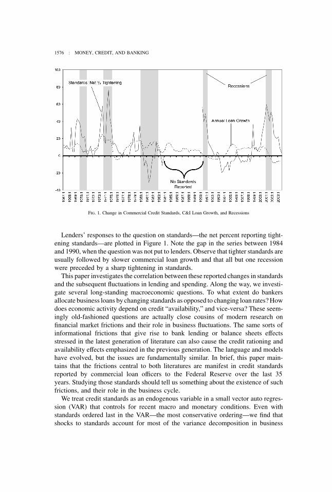
Fig. 1. Change in Commercial Credit Standards, C&I Loan Growth, and Recessions
Lenders’ responses to the question on standards—the net percent reporting tight-ening standards—are plotted in Figure 1. Note the gap in the series between 1984and 1990, when the question was not put to lenders. Observe that tighter standards areusually followed by slower commercial loan growth and that all but one recessionwere preceded by a sharp tightening in standards.
This paper investigates the correlation between these reported changes in standardsand the subsequent fluctuations in lending and spending. Along the way, we investi-gate several long-standing macroeconomic questions. To what extent do bankersallocate business loans by changing standards as opposed to changing loan rates? Howdoes economic activity depend on credit “availability,” and vice-versa? These seem-ingly old-fashioned questions are actually close cousins of modern research onfinancial market frictions and their role in business fluctuations. The same sorts ofinformational frictions that give rise to bank lending or balance sheets effectsstressed in the latest generation of literature can also cause the credit rationing andavailability effects emphasized in the previous generation. The language and modelshave evolved, but the issues are fundamentally similar. In brief, this paper main-tains that the frictions central to both literatures are manifest in credit standardsreported by commercial loan officers to the Federal Reserve over the last 35years. Studying those standards should tell us something about the existence of suchfrictions, and their role in the business cycle.
We treat credit standards as an endogenous variable in a small vector auto regres-sion (VAR) that controls for recent macro and monetary conditions. Even withstandards ordered last in the VAR—the most conservative ordering—we find thatshocks to standards account for most of the variance decomposition in business
CARA LOWN AND DONALD P. MORGAN : 1577
lending, far more than are accounted for bank loan spreads. Innovations in stan-dards also account for a sizable share of the variance decomposition of output.Standards are still significant when we add various proxies for commercial creditquality and demand (business failures) and forward looking variables (forecastedGDP and interest rate spreads). To get some sense of the economic magnitudesinvolved here, we add the standard series to a structural equation for inventoryinvestment, an especially volatile spending component that is closely linked to banklending. Tightenings in standards are a significant drag on retail and wholesaleinventory investment (though not manufacturing). Estimates from the former equa-tions imply that even a moderate tightening in standards—only about half as largeas the typical pre-recession spike in Figure 1—slows the rate of inventory investmentby the same order of magnitude as the overall decline in spending during thetypical recession.
1. THE MEANING OF “STANDARDS”
We use “standards” to refer to any of the various non-price lending terms specifiedin the typical bank business loan or line of credit: collateral, covenants, loan limits,etc. One goal here is to show that the standards series in this paper makes a reasonableindex for the full vector of non-price lending terms. Our concept of standards isclosely tied to the informational frictions that occupy so much of the modernliterature on credit markets. If lenders and borrowers have the same information aboutthe credit risk in a transaction, the risk gets priced and allocated like any other good(or bad)—by price. With asymmetric information, credit gets elevated from a simplequantity-price commodity to a more complicated loan contract with detailed non-price terms.
The notion that the “price” of credit is a vector of terms (not just a simple scalar)goes back some ways in the literature:
A recurrent theme in the literature and among market participants is that the interestalone does not adequately reflect the links between financial markets and the rest ofthe economy. Rather, it is argued, the availability credit and the quality of balancesheets are important determinants of the rate of investment (Blanchard and Fischer,1989, p. 478)
Proponents of the “availability doctrine” in 1950s maintained that monetary policyoperated more through changes in the “availability” of credit than through changesin rates (Roosa 1951), although they failed to explain why a lender would operatethat way (except when constrained by interest rate ceilings). Keeton (1979) andStiglitz and Weiss (1981) showed that “quantity rationing” can result endogenouslyin a variety of models where credit quality varies inversely with the level of interestrates (because of adverse selection or moral hazard among borrowers). Bernankeand Gertler (1989) argue that these frictions wax and wane over the course of
1578 : MONEY, CREDIT, AND BANKING
the business cycle; improved balance sheets during booms induce lenders to easecredit terms, and easier terms prolong the expansion.
Our paper is not strictly a test of any of these models. We invoke them heresimply to establish the possibility that credit conditions warrant attention as apossible factor in business fluctuations. Credit conditions are not just passive reflec-tions of fundamental economic conditions as in a classical model, but rather thecredit cycle can influence the course of the business cycle.
2. MEASURING STANDARDS
The Federal Reserve collects information on bank credit standards in its SeniorLoan Officer Opinion Survey on Bank Lending Practices, a quarterly survey ofmajor banks around the country. The number of participating banks has declined(along with the number of U.S. banking firms in the industry) from about 120 banksin the early years of the survey to roughly 60 today. Participants are typically thelargest banks in their district and are expected to have a sizable share of business loansin their portfolio. In aggregate, participating banks account for about 60% of allloans by U.S. banks and about 70% of all U.S. bank business loans. Questionnairesare transmitted via fax or telephone to participating loan officers by Federal Reserveeconomists in each district, who check responses, follow up as necessary, thentransmit completed surveys back to the Federal Reserve Board economists fortabulation. The response rate is virtually 100%.1
Minor diction changes in the question on standards (p. 1) over the years necessi-tated some splicing to come up with a single series. Starting in 1978, when theprime loan rate emerged as an important benchmark, loan officers were asked toreport separately on standards for loans made at prime rate and for loans at aboveprime. For that period (1978–84), our series is the average of the responses to thetwo questions. The question was dropped from the survey in 1984. Bank interestrates were deregulated about the same time. With unfettered rates, Board decisionmakers may have reasoned that non-price terms, like standards, would matter lessin the loan allocation process (Schreft 1991).2 The question was reinstated in 1990:2 inresponse to concerns about a commercial lending crunch. Since then, lenders
1. Banks are added or replaced as needed, mostly because of mergers between participating banks.The Federal Reserve also conducts occasional ad hoc surveys when market events seem to warrant. Welimit our study to data from the regular survey only. The Senior Loan Officer Opinion Survey compriseda fixed set of 22 questions from its inception in 1964 until 1981. At that time, all but six of those questionswere dropped from the survey to make room for more ad hoc questions on emerging developments. In1984, five of the remaining six core questions were dropped, including the question above. Our splicedseries on C&I standards can be found at http://www.ny.frb.org/rmaghome/economist/morgan/pubs.html(click on Standards). Recent survey results can be found at http://www.federalreserve.gov/boarddocs/SnLoanSurvey/.
2. Interest rate constraints may be sufficient to motivate non-price credit allocation, but are notnecessary; incentive and informational constraints may also lead to such mechanisms. In fact, bank standardsdid become less volatile relative to loan rates after interest rate deregulated (Keeton 1986), suggesting thatinstitutional constraints were part of why lenders resorted to non-price mechanisms.
CARA LOWN AND DONALD P. MORGAN : 1579
have reported separately on standards for small and standards for larger firms; weuse the latter, but the 0.96 correlation between the series makes that choice irrelevant.
The resulting series plotted in Figure 1 is a net percent tightening: the numberof loan officers reporting tightening standards less the number reporting easingdivided by the total number reporting.3,4 Lown, Morgan, and Rohatgi (2000) findthat the standards reported by loan officers are highly negatively correlated withaggregate commercial loan growth and with various measures of economic andbusiness activity. The VAR analysis here takes up where the mostly single-equationmethods in Lown et al. (2000) left off.
3. VAR RESULTS
The core of our VAR comprises just four variables: log real GDP, log GDPdeflator, log commodity prices, and federal funds rate. These four variables representa potentially complete macro economy with “supply” (commodity prices), “demand”(the federal funds rate), output, and prices. Versions of this model have been widelyused in the macro and monetary literature (e.g., Christiano, Eichenbaum, and Evans,1996, Bernanke and Mihov, 1998). We purposely chose an off-the-shelf model inorder to keep attention on the data.
We model the commercial credit market with just two variables: the volume ofcommercial loans at banks and the net percent of loan officers reporting tighteningcommercial credit standards. We ordered the credit variables after the macro vari-ables, with standards last, and loans second-to-last. The VARs include four lagseach of every variable. All models were estimated over the disjoint time period forwhich we have standards data 1968:1–1984:1 and 1990:2–2000:2 (see Table 3for summary statistics).5
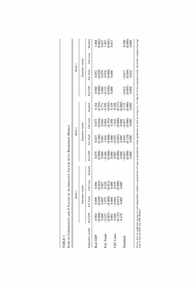
Table 1 reports coefficient sums and significance levels for three VARs. The firstmodel includes C&I loans, but not standards (left panel). Note that past values ofoutput are significant in the loan equation, but loans are insignificant in the outputequation. This confirms the familiar result that output “causes” loans (in the VARsense), but not vice-versa (King 1986, Ramey 1993). Lagged output enters the
3. Weighting the responses over the 1990s by the extent of change (somewhat versus considerably)did not change the picture or the results, nor did using a diffusion index. Integrating the changes reportedby lenders over time did not work as well as any of the other measures.
4. Schreft and Owens (1991) provide an interpretive history of the commercial standards series andnote some dubious features of the data (e.g., the apparent aversion to reporting easings in early year). In aseries of articles, Harris (1973, 1974a, 1974b, 1975) documents a significant, positive correlation betweencommercial credit standards, loan rates and other non-price terms. None of those articles investigates therelationship between standards, lending, and output, however. Duca and Garrett (1995) investigate a relatedseries collected by the Federal Reserve on consumer credit standards. The consumer series is continuous,but its correlation with the commercial series is too low to use it to fill the gap in the commercial series.
5. The Senior Loan Officer Survey is conducted four times per year, but the surveys are not alwaysthree months apart. In those events, we matched the January survey with first quarter observations on theother variables, the May survey with second quarter data, etc. We use the average of the federal fundsrate over the quarter.
TAB
LE
1
Sum
sof
Coe
ffic
ien
tsan
dP
-Val
ues
inA
lter
nat
ive
Vec
tor
Au
toR
egre
ssio
nM
odel
s
Mod
el1
Mod
el2
Mod
el3
Dep
ende
ntva
riab
leD
epen
dent
vari
able
Dep
ende
ntva
riab
le
Inde
pend
ent
vari
able
Rea
lG
DP
Fed.
Fund
sC
&I
Loa
nsSt
anda
rds
Rea
lG
DP
Fed.
Fund
sC
&I
Loa
nsSt
anda
rds
Rea
lG
DP
Fed.
Fund
sC
&I
Loa
nsSt
anda
rds
Rea
lG
DP
0.90
40.
098
0.09
60.
879
0.03
70.
075
0.18
40.
960
0.05
21.
068
(0.0
00)
(0.0
40)
(0.0
45)
(0.0
00)
(0.2
86)
(0.0
44)
(0.5
55)
(0.0
00)
(0.0
28)
(0.0
02)
0.00
00.
005
0.00
70.
000
0.00
10.
040
0.77
10.
000
0.07
90.
027
Fed.
Fund
s�
0.23
71.
075
0.22
9�
0.36
61.
016
0.08
4�
0.29
9�
0.13
30.
978
1.58
7(0
.007
)(0
.000
)(0
.012
)(0
.000
)(0
.000
)(0
.293
)(0
.665
)(0
.020
)(0
.000
)(0
.002
)0.
001
0.00
00.
000
0.00
00.
000
0.39
80.
149
0.00
00.
000
0.01
1C
&I
Loa
ns0.
026
�0.
064
0.93
90.
085
�0.
070
1.01
00.
298
(0.1
25)
(0.0
15)
(0.0
00)
(0.0
00)
(0.0
03)
(0.0
00)
(0.3
37)
0.47
80.
005
0.00
00.
000
0.00
00.
000
(0.0
00)
Stan
dard
s�
0.04
70.
016
�0.
057
0.77
5�
0.01
2�
0.01
70.
580
(0.0
00)
(0.1
24)
(0.0
00)
(0.0
00)
(0.0
95)
(0.0
48)
(0.0
00)
0.00
00.
000
0.00
00.
000
0.00
80.
024
0,00
0
Not
es:
Sum
ofco
effic
ient
son
lags
ofea
chin
depe
nden
tva
riab
leis
repo
rted
first
(P-v
alue
inpa
rent
hese
s).J
oint
sign
ifica
nce
ofea
chse
tof
lags
(i.e
.,P
-val
uefo
rF
-tes
t)re
port
edse
cond
.A
llm
odel
sco
mpr
ise
four
lags
each
oflo
gre
alG
DP,
log
GD
Pde
flato
r.
CARA LOWN AND DONALD P. MORGAN : 1581
loan equation with a positive coefficient sum, implying a procyclical output-loancorrelation. Note also that loans and the federal funds rate cause one another,although the relationship between the two is not necessarily intuitive.
The second VAR includes standards (middle panel). Past standards are highlysignificant in the equations for output and loans, with tightening standards associatedwith lower future levels of loans and output. Note the reverse causality from loansto standards; higher past loan levels are associated with tighter, future standards. Stan-dards and past output are not directly related, but there is an indirect link via thepositive correlation between past output and loans: higher output leads to higherloans, hence higher standards. Controlling for that indirect effect is important;otherwise, we confound the indirect, positive effect of past output on standards (vialoans) with the direct negative effect of standards on future output. We show thisby simply dropping loans from the VAR (right panel). Without loans, past outputappears positively correlated with standards and the link from past standards andoutput is much less negative.6
Impulse Responses. Figure 2 plots impulse responses and standard error bandsfor the VAR model with loans and standards.7 The typical standards shock amounts toan 8% increase in the net fraction tightening, which is significantly different fromzero but substantially less than observed during the 1990 “crunch.” The fractiontightening remains significantly above zero for about three quarters. After aboutnine quarters, lenders commence easing.8 Loans, output, and the federal funds rateall decline significantly in response to the standards shock. Loans contract almostimmediately and continue to decline until bankers start easing standards. At thetrough, loan volume is about 3% lower than before the shock to standards. Outputdeclines significantly in the quarter immediately after the standards shock andremains significantly below its initial rate for almost two years. At its trough, outputis about 0.5% lower than before the shock.9 The federal funds rate also tends tofall after the tightening in standards. The decline becomes significant about threequarters after the shock, by which time the funds rate has been lowered by about50 basis points.
Shocks to both commodity prices and loans cause lenders to tighten standards.Innovations in loans have a prompt, persistent, and significant impact on standards: a
6. Past commodity prices are significant in predicting standards, but not vice-versa. Some of therelationships observed in the VAR without standards change when we add standards. Lagged outputpredicted loans in the model without standards, but not vice-versa. With standards, the causality goes bothways. Loans and the federal funds rates were positively related in the model without standards, not anentirely sensible result. With standards, loans and the funds are not significantly related.
7. The standard error bounds were generated using the Monte Carlo integration program provided inRATS V.5, 2000. See Users Guide (p. 300) and references therein.
8. This seesaw effect makes sense, as loan officers are reporting changes in standards. A change oneway requires an equal and offsetting change in the other direction to return to the normal level of standards.
9. Overall, the path of GDP roughly parallels the path of standards. The decline in GDP becomesinsignificantly different from zero, for example, at about the same time that standards turn significantlynegative (i.e. lenders start easing). The paths of GDP and loan volume are not as close, however. Thetrough in GDP, for example, clearly precedes the low point in loan volume. GDP includes non-businessoutput, of course, and that activity should not necessarily parallel commercial lending.
Fig.
2.Im
puls
eR
espo
nses
for
Cor
eV
AR
CARA LOWN AND DONALD P. MORGAN : 1583
one standard deviation increase in the log of loans (about 1.0%) increases the netfraction tightening by approximately 4.0% two quarters later. Shocks to the federalfunds rate do not affect standards: standards tend upward after an innovation inthe federal funds rate, but the response is never significant.10
Variance Decompositions. Innovations in standards account for nearly a third ofthe error variance in output at four quarters, even more than is attributable toinnovations in the federal funds rate (Table 2). Standards shocks account for aneven larger share of the errors in loans: 15% at three quarters, and nearly two-thirdsat 12 quarters. The feedback from loans to standards, noted earlier, shows up heretoo: innovations in loans account for about 20% of the forecast errors in standards.Ignoring that feedback by omitting loans reduces the share of output shocks attribut-able to standards shocks to less than 10% (at most).11 Shocks to standards accountfor 16% of federal funds innovations at the 12-quarter horizon. In sum, thesedecompositions largely confirm the earlier results: standards are important in account-ing for loans, output, and the federal funds rate, but only loans matter (directly) inaccounting for standards.
Robustness. Differencing GDP, the deflator, commodity prices, and loans did notalter the impulse results in a substantive way, nor did using eight instead of fourlags. Changes in the ordering of the financial variables also did not alter any ofour results. Using industrial production rather than real GDP as the output measureactually strengthens the role of standards, presumably because of the more directlink between commercial credit standards and production. We tested (crudely) forasymmetries in the relationship between standards and output (e.g. tighteningsmatter more than easing) but could not reject symmetry.
4. EXTENDED VARs
The VAR results thus far indicate a strong statistical link between business lendingstandards, business loans, and economic activity, with tightenings in standards fol-lowed by contractions in loans and GDP. While it is tempting to identify the changesin standards with changes in bank loan supply, there is an obvious demand sideinterpretation as well. Tighter standards could signal some other negative distur-bance to economic activity that reduces the demand for loans at the same time bankstighten standards. The cutting edge, however, that reduces loan quantities mightbe the reduction in borrower demand rather than any change in lending standards.Sorting out the correct structural interpretation of our VAR results will likely requirea model. Short of that, we make some headway on the identification issue here byextending the VAR with additional variables that are (arguably) identified with eitherloan demand or supply.
10. We do not include a loan rate because once we control for standards, loan rates (or spreads) haveno additional power for explaining loans or output. Lown and Morgan (2002) find no explanatory role forof standards in the monetary transmission more fully.
11. Ten percent of the innovations in standards is attributable to commodity price shocks (at most).
1584 : MONEY, CREDIT, AND BANKING
TABLE 2
Variance Decompositions
Horizon quarters Real GDP Fed. Funds C&I Loans Standards
Notes: Each panel reports the decomposition of the variance of the forecast error of the series in the panel heading. Figures within panelare the share (%) of the variance at each horizon attributable to the variable in each column. Credit standards enter last in the VAR. SeeTable 1 for VAR model description. Decompositions of commodity prices and deflator and their contributions are not reported. Standarderrors in parentheses.
Our list of proxies, summarized in Table 3, is motivated by a mix of theory,findings elsewhere in the literature, and the reports of loan officers’ themselves.12
Expected output is an obvious fundamental determinant of credit demand; lowerexpected output likely implies lower expected returns on investment and hence,reduced demand for credit.13 Business failures should also serve as reasonable proxyfor demand; with high failures indicating diminished investment prospects and thus,reduced demand for credit. The coverage ratio—interest payments divided by cashflow—is intended to proxy for credit quality as well. The commercial paper-Treasury
12. Since 1990, loan officers that report a change in their commercial credit standards are asked torank five possible reasons for changing standards: economic outlook or uncertainty, expected capitalposition, more or less tolerance for risk, reduced or increased competition from other lenders, changes inspecific sectors.
13. A diminished outlook may also reduce the supply of credit, however, if reduced fundamentalsaggravate incentive problems between banks and borrowers; poorer investment prospects may lead projectowners to shirk on current undertakings or shift effort and resources toward higher mean risk projects.Indeed, loan officers consistently rate “deterioration or increased uncertainty in the outlook” as the mostimportant reason for tightenings in standards. We use the median (across forecasters) of the professionalforecasts compiled by the Federal Reserve Bank of Philadelphia. The data are available on that bank’swebsite.
TAB
LE
3
Dat
aD
efin
itio
ns,
Sum
mar
ySt
atis
tics
,an
dSo
urc
es
Sum
mar
ySt
atis
tics
Var
iabl
eD
efini
tion
Tim
ePe
riod
Obs
Med
ian
SDM
inim
umM
axim
umSo
urce
(s)
Loa
nR
ate
C&
Ilo
anra
te,
annu
aliz
ed19
67:1
–198
3:4
687.
993.
964.
9020
.33
Fede
ral
Res
erve
Boa
rd(m
ode
atba
nks)
Stat
istic
alR
elea
seH
.8:
Ass
ets
and
Lia
bilit
ies
ofC
omm
erci
alB
anks
1990
:2–2
000:
241
7.12
1.29
4.83
10.0
8C
over
age
Rat
ioN
etin
tere
st19
67:1
–198
3:4
6812
.63
3.02
7.11
18.9
8C
omm
erce
Dep
artm
ent
(non
finan
cial
firm
s)pa
ymen
ts/(
net
inte
rest
paym
ents
�ca
shflo
w)
1990
:2–2
000:
241
11.5
13.
449.
9720
.83
Ban
kC
apita
l/Ass
etR
atio
U.S
.ba
nk19
67:1
–198
3:4
680.
050.
010.
020.
07Fl
owof
Fund
sca
pita
l/U.S
.ba
nkas
sets
1990
:2–2
000:
140
0.03
0.01
0.02
0.04
Bus
ines
sFa
ilure
Rat
eL
iabi
litie
sof
faile
d19
67:1
–198
3:4
680.
080.
050.
040.
28D
un&
Bra
dstr
eet
dom
estic
firm
s/gr
oss
prod
uct
ofno
nfina
ncia
lco
rpor
ate
firm
s19
90:2
–199
8:3
340.
210.
280.
081.
15E
xpec
ted,
Rea
lG
DP
Four
-qua
rter
ahea
d19
68:4
–198
3:4
617.
170.
316.
607.
39Fe
dera
lR
eser
veB
ank
offo
reca
sted
GD
PPh
ilade
lphi
a(m
edia
nfo
reca
st)
1990
:2–2
000:
241
8.63
0.25
8.33
9.16
Pape
r-bi
llSp
read
Six-
mon
thco
mm
erci
al19
67:1
–198
3:4
680.
730.
620.
033.
51Fe
dera
lR
eser
veB
oard
pape
rra
te(n
onfin
anci
al).
Stat
istic
alR
elea
seT-
bill
rate
(six
-mon
thH
.15:
Sele
cted
until
1971
;(t
hree
mon
ths
Inte
rest
Rat
esaf
ter
1971
)19
90:2
–200
0:2
410.
430.
160.
180.
91
(Con
tinu
ed)
TAB
LE
3
Con
tin
ued
Sum
mar
ySt
atis
tics
Var
iabl
eD
efini
tion
Tim
ePe
riod
Obs
Med
ian
SDM
inim
umM
axim
umSo
urce
(s)
Com
mod
ityPr
ice
Inde
xJO
C-E
CR
Iin
dust
rial
1967
:1–1
983:
468
53.1
521
.25
27.0
087
.90
DL
X,
USE
CO
Npr
ice
inde
x,sp
otin
flatio
nra
tesm
ooth
ed,
annu
aliz
ed(1
996
�10
0)19
90:2
–200
0:2
4188
.70
7.93
79.5
010
6.50
GD
PB
illio
nsof
chai
ned
1967
:1–1
983:
468
4364
.20
630.
2434
64.1
055
90.5
0D
LX
,U
SEC
ON
(GD
PH)
2000
dolla
rs,
quar
terl
y,SA
AR
1990
:2–2
000:
241
7988
.00
859.
2770
40.8
098
47.9
0G
DP
Defl
ator
Impl
icity
pric
e19
67:1
–198
3:4
6837
.96
13.4
023
.61
66.0
1D
LX
,U
SEC
ON
(DG
DP)
defla
tor,
quar
terl
y,SA
(200
0�
100)
1990
:2–2
000:
241
91.8
65.
2581
.31
99.7
5Fe
dera
lFu
nds
Rat
eE
ffec
tive
rate
,p.
a.%
1967
:1–1
983:
468
7.55
3.65
3.55
17.7
9D
LX
,U
SEC
ON
(FFE
D)
1990
:2–2
000:
241
5.31
1.30
2.99
8.24
Stan
dard
sN
etpe
rcen
tage
of19
67:1
–198
3:4
680.
070.
19�
0.31
0.77
Seni
orL
oan
Offi
cer
dom
estic
resp
onde
nts
Opi
nion
Surv
eyon
tight
enin
gst
anda
rds
Ban
kL
endi
ngPr
actic
esfo
rC
&I
loan
s(l
arge
and
med
ium
bank
son
ly)/
100
1990
:2–2
000:
241
0.00
0.18
�0.
190.
57C
&I
Loa
nsB
illio
nsof
1967
:1–1
983:
468
184.
7299
.68
80.5
341
5.43
Fede
ral
Res
erve
Boa
rddo
llars
,m
onth
lySt
atis
tical
Rel
ease
H.1
5:Se
lect
edIn
tere
stR
ates
1990
:2–2
000:
241
694.
6314
2.16
590.
5310
48.8
3
CARA LOWN AND DONALD P. MORGAN : 1587
TABLE 4
Coefficients Sums and P-Values in Extended Vector Auto Regression (VAR)
Dependent variable: Dependent variable:
Independent variable: Real GDP C&I Loans Standards Independent variable: Real GDP C&I Loans Standards
Var models include the core variables described in Table 1, plus the variable indicated below. Reported is the sum of coefficients on lagsof each independent variable (P-value in parentheses). Also reported third is P-value for F-test of whether the coefficients are jointly zero.
bill spread is another forward looking variable, with spikes serving as a (usually)reliable signal of future contractions in activity.14 We included capital/asset ratiosat banks as a potential determinant of bank loan supply.15 We also add a loan rate,or spread, to see which variable—standards or loan rates—seems most importantin explaining loan levels. The extra variables are added one at a time to the VAR,and in the penultimate position (before standards, but after every other variable).
Table 4 reports abbreviated sets of exclusion tests for each of the extended VARs.Even with the extra variables in the models, standards remain highly significantin predicting loans and output, in fact, most of the extra other variables pale incomparison. Given standards, lagged loan rates are insignificant in predicting output.Lagged loan rates are significant (by the F-test) in predicting loan levels, but thesum of coefficients on the lagged loans rates is insignificant. Past values of the interest-coverage ratio are marginally significant in predicting real GDP, but less so thanstandards.
Of the extra variables, only the business failures rate is significant in explainingstandards. A higher rate of failures is associated with tightening standards, as one
14. Researchers have identified changes in the spreads with changes in monetary policy, increases inthe extent of information problems, and simply increased risk or decreased risk tolerance.
15. In Bernanke and Gertler (1987), for example, capital is an essential determinant of banks’ lendingcapacity; adverse capital shocks force banks to substitute safe securities for riskier loans in order to satisfymarket imposed capital requirements. Capital is also rated high by loan officers as a reason for changesin standards.
1588 : MONEY, CREDIT, AND BANKING
would expect. Given the failure rate, the current change in standards is related toits own past changes at only the 10% level, indicating that failures absorb some ofthe impact of lagged standards. Even controlling for the failure rate, however,standards are still highly significant in predicting loans and output, while the failurerate is not significant in either equation.16
We investigated the VAR with the business failure rate in further detail, sincethis variable proved significant in explaining standards. The impulse responsesfrom the model reveal that shocks to the failure rate are followed by a significanttightening in credit standards (Figure 3, lower right). Even after accounting for theeffect of failures on standards, however, a standards shock still causes output toslow significantly.17
Innovations in the failure rate account for about 10% of the variance decompositionof standards. The share of the variance decomposition of output attributable toinnovations in standards is lower when the model includes business failures, butstill sizable (Table 5). The share attributable to standards increases to about 15%at four quarters, and declines thereafter. Similarly, the importance of standards inexplaining the variance decomposition of lending falls somewhat, but is still quitelarge: 18% at four quarters and 28% at eight quarters.
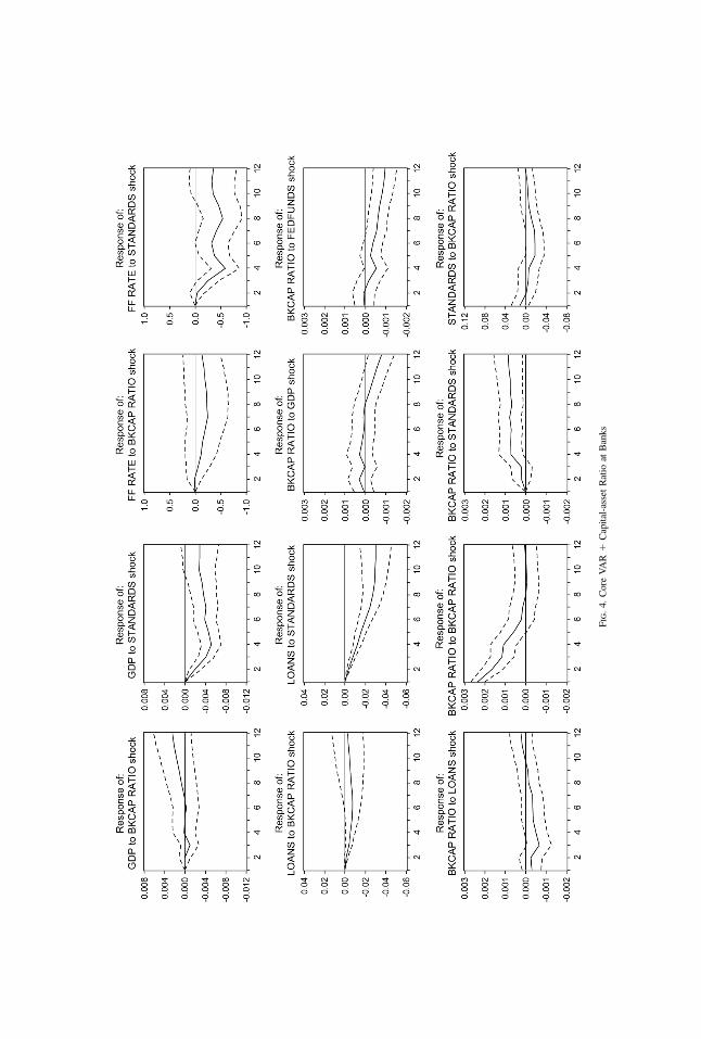
More on Bank Capital. Although the predicted negative relationship betweenstandards and capital ratios did not materialize in the exclusion tests, the strongtheoretical priors for a role of capital motivated further investigation of this variablein the model. Examining the impulse response and variance decompositions mayuncover indirect links between the variables via feedback among other variables inthe VAR. In fact, positive shocks to the capital/asset ratio are somewhat expansionaryin terms of lending standards (Figure 4, lower right). The response of standards ismarginally significant (between 5% and 10%) four quarters after the initial shockand for several quarters thereafter. According to the variance decompositions (Table5), however, shocks to the capital/asset ratio account for only 8% of the variancedecomposition of standards at eight quarters. Again, we view this mixed-to-weakresult more as a problem with using book-value capital series than as evidenceagainst the notion that capital positions can sometimes constrain bank lending.18
In sum, the significance of the business failure rate in explaining credit standardsprovides some support for the idea that standards are altered in response to changes infirms’ financial health. The marginal significance of bank capital suggests somerole for bank balance sheet health as well. Yet even with the inclusion of these determi-nants of credit standards, the remaining unexplained or exogenous part of standardsappears to play a significant role in accounting for movements in lending and output.
16. The insignificant relationship between bank capital ratios and standards might partly reflect ouruse of book capital rather than market capital. We are also missing data for 1984–90, when banks wereanticipating tightening capital constraints under the Basle Accord.
17. The VAR ordering is standards last and failures second-to-last, so the innovation in standards isorthogonal to the contemporaneous innovation in failures.
18. We have also considered other bank variables such as the ratio of nonperforming loans to totalloans and an index of bank stock prices. These variables were not significant in explaining standards, nordid they displace standards in explaining output or loans.
Fig.
3.C
ore
VA
R�
Non
-fina
ncia
lB
usin
ess
TABLE 5
Variance Decompositions from Extended VARs
I. VAR with Business Failure Rate
A. Percentage of GDP variance attributed to shocks to:
Horizon quarters Real GDP Fed. Funds C&I Loans Business Failures Standards
Notes: Reported in each panel is the decomposition of the variance of the forecast error of the series in the panel heading. Each cellwithin a panel reports the percentage of the variance at each horizon attributable to shocks in the variable in each column.
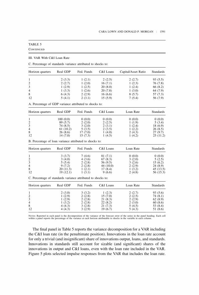
The final panel in Table 5 reports the variance decomposition for a VAR includingthe C&I loan rate (in the penultimate position). Innovations in the loan rate accountfor only a trivial (and insignificant) share of innovations output, loans, and standards.Innovations in standards still account for sizable (and significant) shares of theinnovations in output and C&I loans, even with the loan rate included in the VAR.Figure 5 plots selected impulse responses from the VAR that includes the loan rate.
Fig.
4.C
ore
VA
R�
Cap
ital-
asse
tR
atio
atB
anks
Fig.
5.C
ore
VA
R�
C&
IL
oan
Rat
e
1594 : MONEY, CREDIT, AND BANKING
The loan rate responds strongly and positively to innovations in output. Shocks tothe loan rate cause loans to contract slightly, but the loan response is very brief,especially by comparison with the response of loans to a shock in standards.
5. STANDARDS IN A STRUCTURAL INVENTORY INVESTMENT MODEL
We estimate a structural equation for inventory investment and measure thequantitative effect of a tightening in standards on inventory investment. The structuralpart of the equation is intended to explicitly control for inventory investment demandso the coefficients on standards should measure the quantitative impact of a reductionin the supply of bank credit (via tighter standards) on investment. A similar strategywas used in the exploration of the “mix” variable by Kashyap, Stein, and Wilcox(1993). Inventory spending makes the ideal laboratory for this examination because(1) banks fund a substantial share of inventory investment, (2) fluctuations in inventoryinvestment figure disproportionately in GDP fluctuations, and (3) inventory investmentspending is curiously insensitive to interest rates (Blinder and Maccini 1991). Afinding that fluctuations in commercial credit standards affect inventory investmentmay help explain (2) and (3).
The inventory investment equation—a simple target adjustment of Lovell (1961)—issimilar to the version in Gertler and Gilchrist (1994):
where I, S,and ST denote the logs of inventories, sales and loan standards, and rdenotes the short-term real interest rate. The dependent variable is the inventorygrowth rate. According to the usual model, inventory investment of each perioddepends on the gap between the lagged level of inventories and the target level of(expected) sales and on the short-term interest rate. Short-run dynamics are allowedvia the lagged differences of all variables. The difference in our equation is the additionof commercial credit standards on the right-hand side. Given inventory investmentdemand, we expect slower rates of investment when standards have been tight.
As is common, we use actual sales in lieu of expected sales on the right-hand side.Since current sales are endogenous, we use lagged values of sales and all the othervariables (including standards) as instruments for current sales.19 For the real interestrate, we use the prime loan rate less the one-year inflation rate. We estimate Equation(1) separately for each category of inventories: retail, wholesale, and manufacturing.For each category, we include the corresponding category of sales on the right-hand side.
19. Including standards as an instrument eliminates the possible criticism that loan standards aresignificant in explaining inventories because they contain information about expected sales.
CARA LOWN AND DONALD P. MORGAN : 1595
TABLE 6
Structural Inventory Investment Regression Equations with Credit Standards
Reported are regression coefficients (standard errors). Dependent variable is inventory investment of type indicated. The dependent variableis the growth rate of the respective inventory category. I and S denote the logarithm of the inventory and sales category, respectively.Real is the level of the Prime Rate less the one-year inflation rate. Standards is the level of loan standards. The equations are estimatedusing instrumental variables with (St�1–It�1), Realt�1, Standardst�1, ∆ It�1, ∆ St�1, ∆Realt�1, ∆Standardst�1 as instruments. Standard errorsare in parentheses. * and ** indicate significance at the 5% and 1% levels, respectively.
Table 6 presents the estimates of the inventory investment equations. Thoughinsignificant in the equation for manufacturing, standards are highly significant in theequations for trade inventories.20 We can reject that the standards coefficients are jointlyzero in the wholesale inventory equation at the 6% level. The irrelevance of standardsin the retail inventory equation can be rejected at 2%. Excluding standards from theretail inventory equation reduces the adjusted R2 by about half, indicating that fluctua-tion in standards account for about half of the explanatory power of the retail inventoryinvestment equation.
The impact of a change in standards on inventory investment in the trade sectorsis large relative to the normal behavior of those series. One standard deviation tight-ening in standards (about 19 percentage points) reduces retail inventory investment by1.5 percentage points per year (compared to a mean rate of 3.9 per year; standarddeviation of 6.2%) and wholesale inventory by 1.3 percentage points per year(compared to a mean of 5.2%, standard deviation of 5.6%). In absolute terms, thistightening would trim trade inventory investment on the order of $10 billion. Thatnumber is substantial relative to the $30 billion drop in real GDP during the typicalrecession. Bear in mind also that the tightening in this experiment is gentle relativeto the usual 40% net tightening before recessions (Figure 1).
20. We do not know why standards appear irrelevant for manufacturing inventories. The typical manufac-turing firms may be larger (than the typical trade firm) and may be less bank-dependent for credit.Decomposing manufacturing inventories (by stage of fabrication) might reveal effects of standards onwork-in-progress and raw material inventories.
1596 : MONEY, CREDIT, AND BANKING
6. CONCLUSIONS
Fluctuations in commercial credit standards are highly significant in predictingcommercial bank loans, real GDP, and inventory investment in the trade sector. Ifstandards are tightening more than usual (given macro and credit conditions), lowerlevels of loans and slower rates of output can be expected with a high degree ofconfidence. Credit standards are far more informative about future lending than areloan rates, which is consistent with the idea that some sort of friction in lendingmarkets leads lenders to ration loans via changes in standards more than throughchanges in rates.
We hesitate to interpret these correlations as evidence of a causal connection betweenbank loan supply and real activity as tightenings in standards may merely signal (asopposed to cause) an incipient slowdown. It is notable, however, that shocks tostandards still affect lending and output in extended VAR models that control forrecent macroeconomic conditions and firm and bank financial health. Standards arealso significant in structural inventory investment equations, where the role of standardsis (arguably) identified with changes in the supply of credit.
We found feedback from loans to standards, suggesting a sort of credit cycle.Higher loan levels cause tightening standards, perhaps because lenders conclude (orare told by supervisors) that standards are too loose. Tighter standards are followedby lower spending and loan levels, which eventually cause easing standards and higherspending and loan levels . . . ad infinitum.
Some of the negative findings here are also interesting. Shocks to the federal fundsrate do not cause changes in standards, lenders simply raise loan rates more or less instep with the funds rate. While this finding seems to counter theories of a narrowbank lending channel of monetary policy, at least via changes in standards, furtherresearch using alternative monetary policy measures may yet uncover a standardschannel. We found a negative relationship between banks’ capital ratios and theirlending via standards but that link between bank capital and lending standards wasstatistically weak. We view this more as a problem with book capital measures thanwith theories of capital constraints on banks. The federal funds rate falls in responseto positive shocks in credit standards, suggesting that monetary policymakers followa “lean-against-the-lenders” strategy.
LITERATURE CITED
Bernanke, Ben, and Mark Gertler (1987). “Banking and Macroeconomic Equilibrium.” In NewApproaches to Monetary Economics, edited by I. Barnett and K. Singleton. Cambridge:Cambridge University Press.
Bernanke, Ben, and Mark Gertler (1989). “Agency Costs, Net Worth and Business Fluctuations.”American Economic Review 79, 14–31.
Bernanke, Ben S., and Ilian Mihov (1998). “Measuring Monetary Policy.” Quarterly Journalof Monetary Policy CXIII, 869–902.
CARA LOWN AND DONALD P. MORGAN : 1597
Blanchard, Olivier, and Stanley Fischer (1989). Lectures in Macroeconomics. MIT Press,Cambridge, MA: MIT Press.
Blinder, Alan S., and Louis J. Maccini (1991). “Taking Stock: A Critical Assessment of RecentResearch on Inventories.” Journal of Economic Perspectives V, 73–96.
Christiano, Lawrence, Martin Eichenbaum, and Charles Evans (1996). “The Effects of MonetaryPolicy Shocks: Evidence from the Flow of Funds.” Review of Economics and Statistics 78,16–34.
Gertler, Mark, and Simon Gilchrist (1994). “Monetary Policy, Business Cycles, and the Behaviorof Small Manufacturing Firms.” Quarterly Journal of Economics 109, 309–340.
Harris, Duane G. (1973). “Some Evidence on Differentiated Lending Practices at CommercialBanks.” Journal of Finance 28, 1302–1311.
Harris, Duane G. (1974a). “Interest Rates, Nonprice Terms, and the Allocation of Bank Credit.”Southern Economic Journal 40, 428–433.
Harris, Duane G. (1974b). “Credit Rationing at Commercial Banks: Some Empirical Evidence.”Journal of Money, Credit, and Banking 6, 227–240.
Kashyap, Anil, Jeremy Stein, and David Wilcox (1993). “Monetary Policy and Credit Condi-tions: Evidence from the Composition of External Finance.” American Economic Review83, 78–99.
Keeton, William R. (1979). Equilibrium Credit Rationing. New York: Garland, 1979.
Keeton, William R. (1986). “Deposit Rate Deregulation, Credit Availability, and MonetaryPolicy.” Federal Reserve Bank of Kansas City Economic Review, 26–42.
Lown, Cara S., Don Morgan, and Sonali Rohatgi (2000). “Listening to Loan Officers: TheImpact of Commercial Credit Standards on Lending and Output.” Federal Reserve Bank ofNew York Economic Policy Review 6, 1–16.
Lown, Cara S., and Don Morgan (2002). “Credit Effects in the Monetary Mechanism.” FederalReserve Bank of New York Economic Policy Review 8, 217–235.
Lovell, M. (1961). “Manufacturers Inventories, Sales Expectations, and the Acceleration Princi-ple.” Econometrica XXIX, 293–314.
Ramey, Valerie (1993). “How Important is the Credit Channel in the Transmission of MonetaryPolicy?” Carnegie-Rochester conference Series on Public Policy 39, 1–45.
Roosa, Robert V. (1951). “Interest Rates and the Central Bank.” In Money, Trade and EconomicGrowth: Essays in Honor of John H. Williams. New York: Macmillan.
Schreft, Stacey L., and Raymond E. Owens (1991). “Survey Evidence of Tighter CreditConditions: What Does It Mean?” Federal Reserve Bank of Richmond Economic Review29–34.
Stiglitz, Joseph E., and Andrew Weiss (1981). “Credit Rationing in Markets in ImperfectInformation.” American Economic Review 71, 393–410.