The Cricket Indoor Location System by Nissanka Bodhi Priyantha S.M. Computer Science, Massachusetts Institute of Technology (2001) B.S. Electronic Engineering, University of Moratuwa, Sri Lanka (1996) Submitted to the Department of Electrical Engineering and Computer Science in partial fulfillment of the requirements for the degree of Doctor of Philosophy in Computer Science and Engineering at the MASSACHUSETTS INSTITUTE OF TECHNOLOGY June 2005 c Massachusetts Institute of Technology 2005. All rights reserved. Author .............................................................. Department of Electrical Engineering and Computer Science May 19, 2005 Certified by .......................................................... Hari Balakrishnan Associate Professor of Computer Science and Engineering Thesis Supervisor Accepted by ......................................................... Arthur C. Smith Chairman, Department Committee on Graduate Students
Transcript
The Cricket Indoor Location System
by
Nissanka Bodhi Priyantha
S.M. Computer Science, Massachusetts Institute of Technology (2001)B.S. Electronic Engineering, University of Moratuwa, Sri Lanka (1996)
Submitted to the Department of Electrical Engineering and ComputerScience
in partial fulfillment of the requirements for the degree of
Doctor of Philosophy in Computer Science and Engineering
Chairman, Department Committee on Graduate Students
2
The Cricket Indoor Location Systemby
Nissanka Bodhi Priyantha
Submitted to the Department of Electrical Engineering and Computer Scienceon May 19, 2005, in partial fulfillment of the
requirements for the degree ofDoctor of Philosophy in Computer Science and Engineering
Abstract
Indoor environments present opportunities for a rich set of location-aware applicationssuch as navigation tools for humans and robots, interactive virtual games, resourcediscovery, asset tracking, location-aware sensor networking etc. Typical indoor appli-cations require better accuracy than what current outdoor location systems provide.Outdoor location technologies such as GPS have poor indoor performance becauseof the harsh nature of indoor environments. Further, typical indoor applicationsrequire different types of location information such as physical space, position andorientation.
This dissertation describes the design and implementation of the Cricket indoorlocation system that provides accurate location in the form of user space, positionand orientation to mobile and sensor network applications.
Cricket consists of location beacons that are attached to the ceiling of a building,and receivers, called listeners, attached to devices that need location. Each beaconperiodically transmits its location information in an RF message. At the same time,the beacon also transmits an ultrasonic pulse. The listeners listen to beacon transmis-sions and measure distances to nearby beacons, and use these distances to computetheir own locations. This active-beacon passive-listener architecture is scalable withrespect to the number of users, and enables applications that preserve user privacy.
This dissertation describes how Cricket achieves accurate distance measurementsbetween beacons and listeners. Once the beacons are deployed, the MAT and AFLalgorithms, described in this dissertation, use measurements taken at a mobile listenerto configure the beacons with a coordinate assignment that reflects the beacon layout.This dissertation presents beacon interference avoidance and detection algorithms, aswell as outlier rejection algorithms to prevent and filter out outlier distance estimatescaused by uncoordinated beacon transmissions.
The Cricket listeners can measure distances with an accuracy of 5 cm. The listen-ers can detect boundaries with an accuracy of 1 cm. Cricket has a position estimationaccuracy of 10 cm and an orientation accuracy of 3 degrees.
Thesis Supervisor: Hari BalakrishnanTitle: Associate Professor of Computer Science and Engineering
3
4
To my parents.
5
6
Acknowledgments
Hari Balakrishnan has been more than a perfect advisor during my life at MIT—hehas been an advisor, mentor, and a good friend. His energy and enthusiasm stillcontinue to amaze me. During the countless discussions I had with him, I always feltthat I was his only student, although he had about ten students.
Seth Teller provided much guidance in the research leading to this dissertationand played a key role in shaping the Cricket system. His continued focus on thepractical aspects and applications was an important factor in the impact this projecthas had. I thank him for serving on my committee.
Robert Morris provided valuable feedback during the writing of this dissertation.I thank him for serving on my committee.
Despite my lack of knowledge in the field of computational geometry, Erik De-maine patiently discussed the correctness of some of the theorems described in thisdissertation.
I thank John Guttag for providing me financial assistance and advice when I firstjoined MIT. He has continued to be a great inspiration during my life at MIT.
This dissertation presents joint work with Hari Balakrishnan, Anit Chakraborty,Erik Demaine, Allen Miu, and Seth Teller. A number of people have contributedto the Cricket project. Cricket started from my joint work with Hari Balakrishnanand Anit Chakraborty. Dorothy Curtis, Allen Miu, and Ken Steele subsequentlycontributed to the development of the Cricket system. John Ankcorn, apart fromcontributing to the Cricket project, also proofread portions of this dissertation andhelped me survive the summers I spent in California. Michel Goraczko handled theTinyOS port of the Cricket firmware, and did an excellent job of responding to userquestions, producing (with Hari Balakrishnan and Allen Miu) the user manual, andmaintaining the inventory of Cricket hardware. He also always managed to find meenough Crickets whenever I wanted to run a large-scale experiment. David Moore alsocontributed to the development of cricket firmware. Adam Smith implemented theKalman filter-based position tracking algorithms in Cricket. Crossbow Technologiesmanufactured the current version of the Cricket hardware. I thank Roshan Baliga,Nikos Michalakis, Jorge Nogueras, and Kevin Wang for using Cricket for their thesiswork and providing valuable feedback. I thank Anant Agarwal, Stephen Garland,and Larry Rudolph for using Cricket in their pervasive computing course at MIT. Ialso thank many users around the world for building systems and applications usingthe Cricket platform.
I thank my colleagues Dave Anderson, Magdelena Balaziska, Vladimir Bychkovsky,Nick Feamster, Bret Hull, Kyle Jamieson, Jaeyeon Jung, Stanislav Rost, EugeneShih, Ali Shoeb, Alex Snoeren, Godfrey Tan, and Michael Walfish in the Networksand Mobile Systems group for providing a fun and exciting working environment.Other friends from the fifth floor of LCS, Steven Bauer, Chandrasekhar Boyapati,Dina Katabi, Jinyang Li, Athicha Muthitacharoen, Xiaowei Yang, and Yan Zhangenriched my life at MIT. I thank my roommate Lik Mui for the countless discussionswe had on deep philosophical issues while sharing a room at Ashdown for severalyears.
7
The people I met when I first came to MIT made adjusting to a new countryeasy—in particular, William Adjie-Winoto, Deepak Bansal, Jeremy Lilley, HariharanRahul, and Suchitra Raman created a friendly working environment during my earlydays at MIT.
This work was supported by the National Science Foundation and by the MITProject Oxygen partnership (Acer Inc., Delta Electronics Inc., HP Corp., NTT Inc.,Nokia Research Center, and Philips Research).
I thank my beloved wife Kusala for providing continued support and encourage-ment during past several years. I thank our baby daughter Dilini for being a stringreason to finish this thesis and for sleeping throughout the night since the day shewas born.
I dedicate this thesis to my parents who have dedicated their entire life for myeducation.
5.4.1 Orientation from Three Beacons and Two Receiver Arrays . . 1155.4.2 Orientation from Two Beacons and an Inclinometer . . . . . . 1165.4.3 Orientation of a Horizontal Listener . . . . . . . . . . . . . . . 118
1-1 A screen shot of a navigation application built using Cricket. . . . . . 231-2 A Cricket node with a sensor board attached to it. . . . . . . . . . . . 241-3 A screen shot of an interactive version of the Doom game (with per-
mission of Prof. Larry Rudolph.) . . . . . . . . . . . . . . . . . . . . 251-4 A Cricket hardware unit; this unit can function as either a beacon or
2-1 Offset β between the aircraft heading and the direction of the VORstation is given by β = π + θ−α, where θ is the bearing of the aircraftto the VOR ground station and α is the aircraft heading. . . . . . . . 36
2-2 A VOR ground station transmits a stationary omni-directional fre-quency modulated signal S1 and a rotating directional signal. Aircraftscalculate their bearing to the VOR station by measuring the time shiftbetween a time stamp on S1 and the peak of S2. . . . . . . . . . . . . 37
2-3 Computing the position based on intersecting hyperbolas in the LO-RAN system. . . . . . . . . . . . . . . . . . . . . . . . . . . . . . . . 38
2-4 Node coordinates can be assigned by measuring the distance from in-dividual coordinate axes. . . . . . . . . . . . . . . . . . . . . . . . . . 43
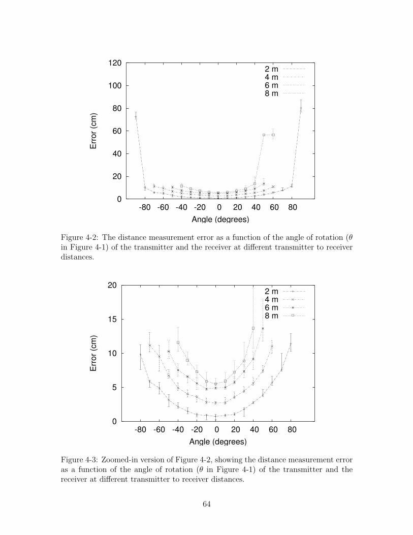
4-2 The distance measurement error as a function of the angle of rota-tion (θ in Figure 4-1) of the transmitter and the receiver at differenttransmitter to receiver distances. . . . . . . . . . . . . . . . . . . . . 64
4-3 Zoomed-in version of Figure 4-2, showing the distance measurementerror as a function of the angle of rotation (θ in Figure 4-1) of thetransmitter and the receiver at different transmitter to receiver distances. 64
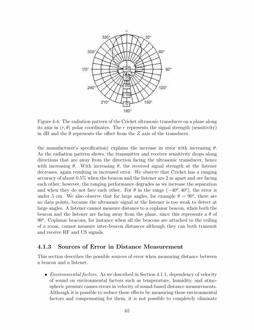
4-4 The radiation pattern of the Cricket ultrasonic transducer on a planealong its axis in (r, θ) polar coordinates. The r represents the signalstrength (sensitivity) in dB and the θ represents the offset from the Zaxis of the transducer. . . . . . . . . . . . . . . . . . . . . . . . . . . 65
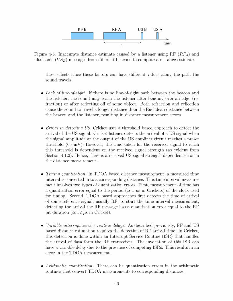
4-5 Inaccurate distance estimate caused by a listener using RF (RFA) andultrasonic (USB) messages from different beacons to compute a dis-tance estimate. . . . . . . . . . . . . . . . . . . . . . . . . . . . . . . 66
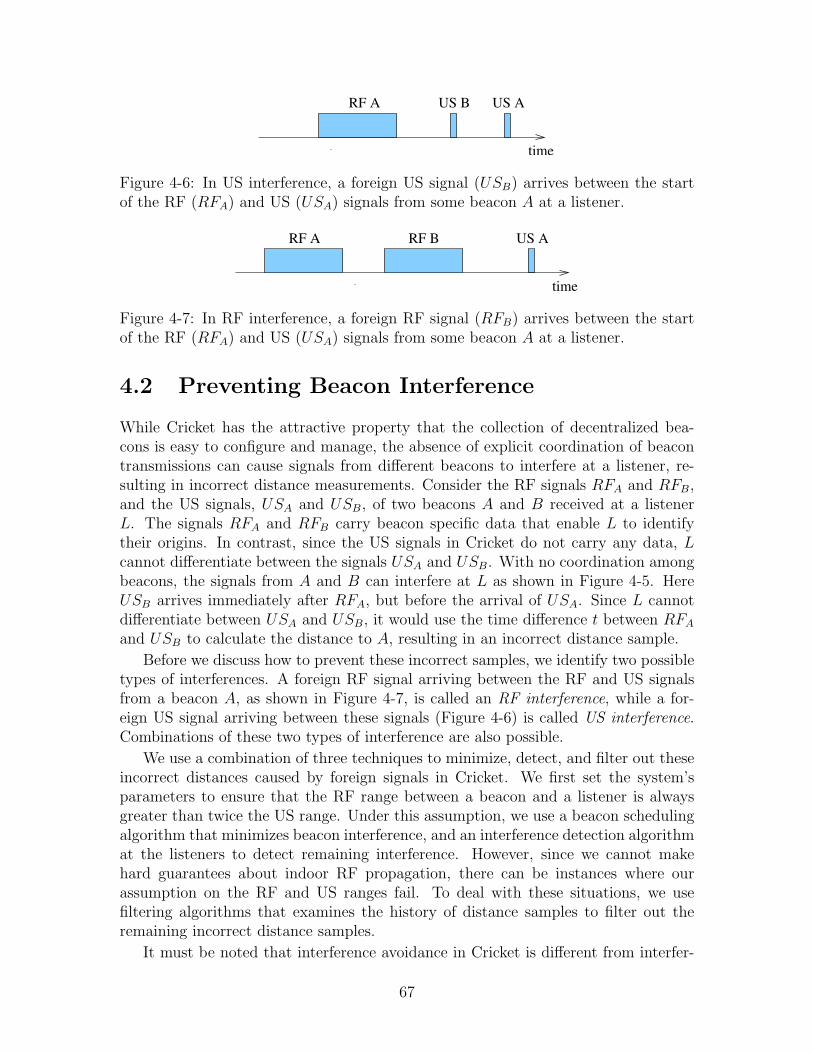
4-6 In US interference, a foreign US signal (USB) arrives between the startof the RF (RFA) and US (USA) signals from some beacon A at a listener. 67
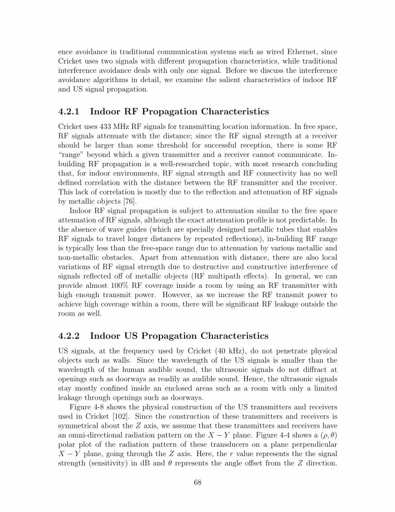
4-7 In RF interference, a foreign RF signal (RFB) arrives between the startof the RF (RFA) and US (USA) signals from some beacon A at a listener. 67
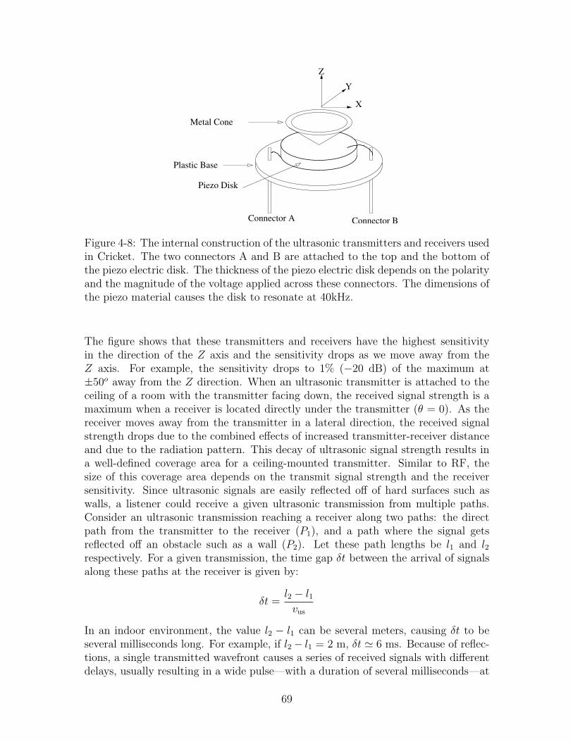
4-8 The internal construction of the ultrasonic transmitters and receiversused in Cricket. The two connectors A and B are attached to the topand the bottom of the piezo electric disk. The thickness of the piezoelectric disk depends on the polarity and the magnitude of the voltageapplied across these connectors. The dimensions of the piezo materialcauses the disk to resonate at 40kHz. . . . . . . . . . . . . . . . . . . 69
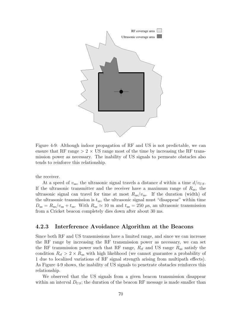
4-9 Although indoor propagation of RF and US is not predictable, we canensure that RF range > 2 × US range most of the time by increasingthe RF transmission power as necessary. The inability of US signalsto permeate obstacles also tends to reinforce this relationship. . . . . 70
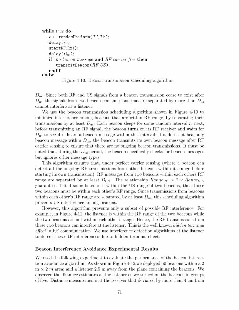
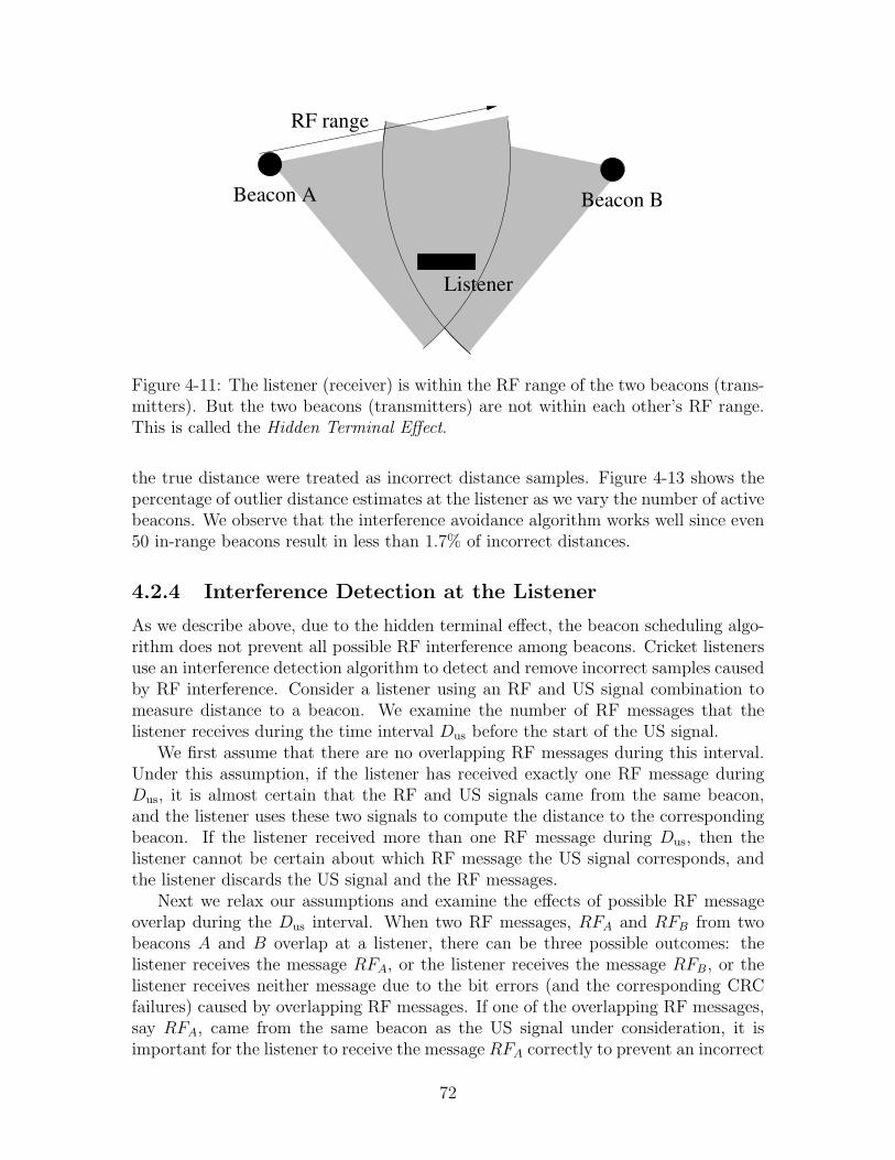
4-11 The listener (receiver) is within the RF range of the two beacons(transmitters). But the two beacons (transmitters) are not within eachother’s RF range. This is called the Hidden Terminal Effect. . . . . . 72
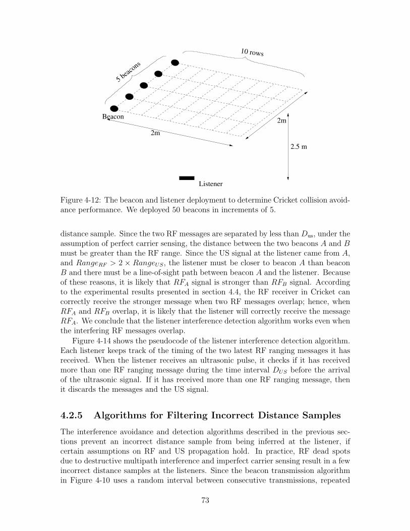
4-12 The beacon and listener deployment to determine Cricket collisionavoidance performance. We deployed 50 beacons in increments of 5. . 73
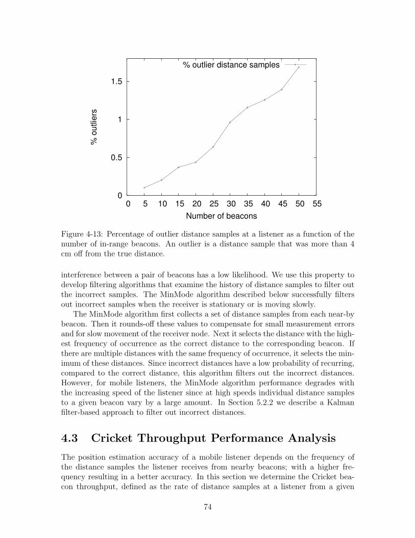
4-13 Percentage of outlier distance samples at a listener as a function of thenumber of in-range beacons. An outlier is a distance sample that wasmore than 4 cm off from the true distance. . . . . . . . . . . . . . . . 74
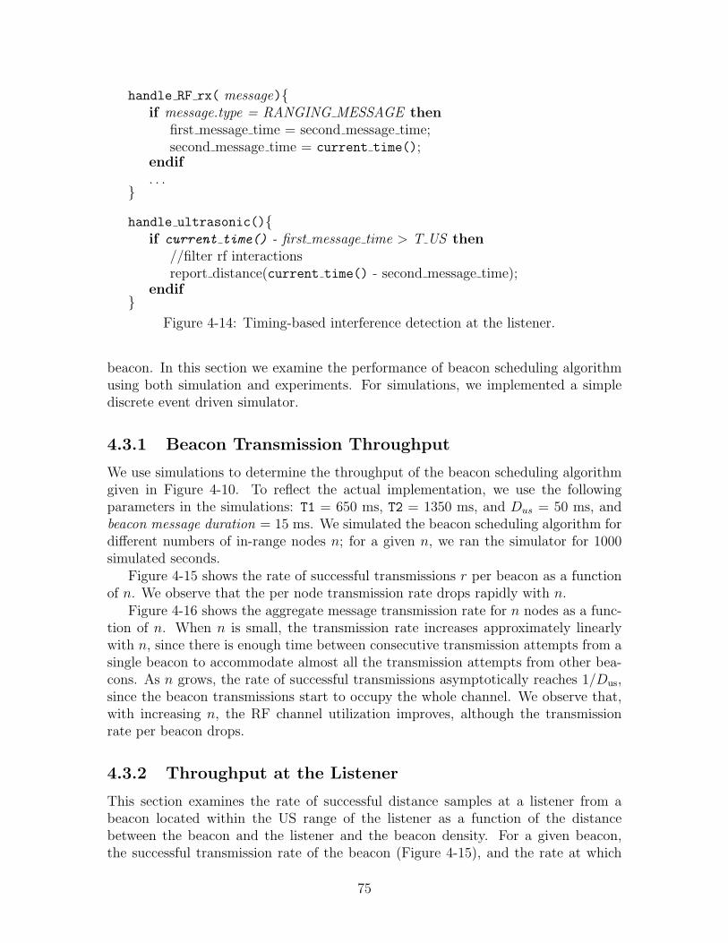
4-14 Timing-based interference detection at the listener. . . . . . . . . . . 75
14
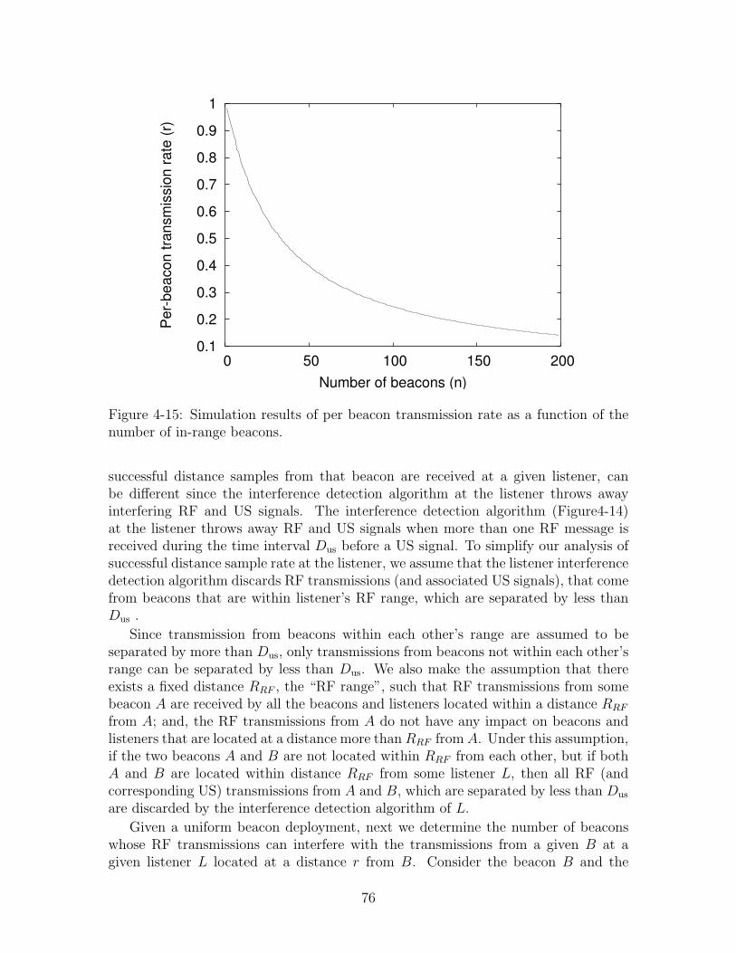
4-15 Simulation results of per beacon transmission rate as a function of thenumber of in-range beacons. . . . . . . . . . . . . . . . . . . . . . . . 76
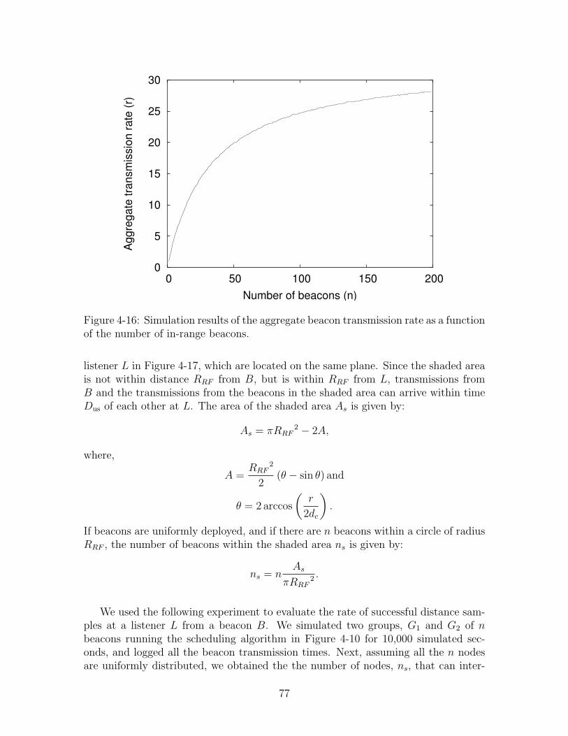
4-16 Simulation results of the aggregate beacon transmission rate as a func-tion of the number of in-range beacons. . . . . . . . . . . . . . . . . . 77
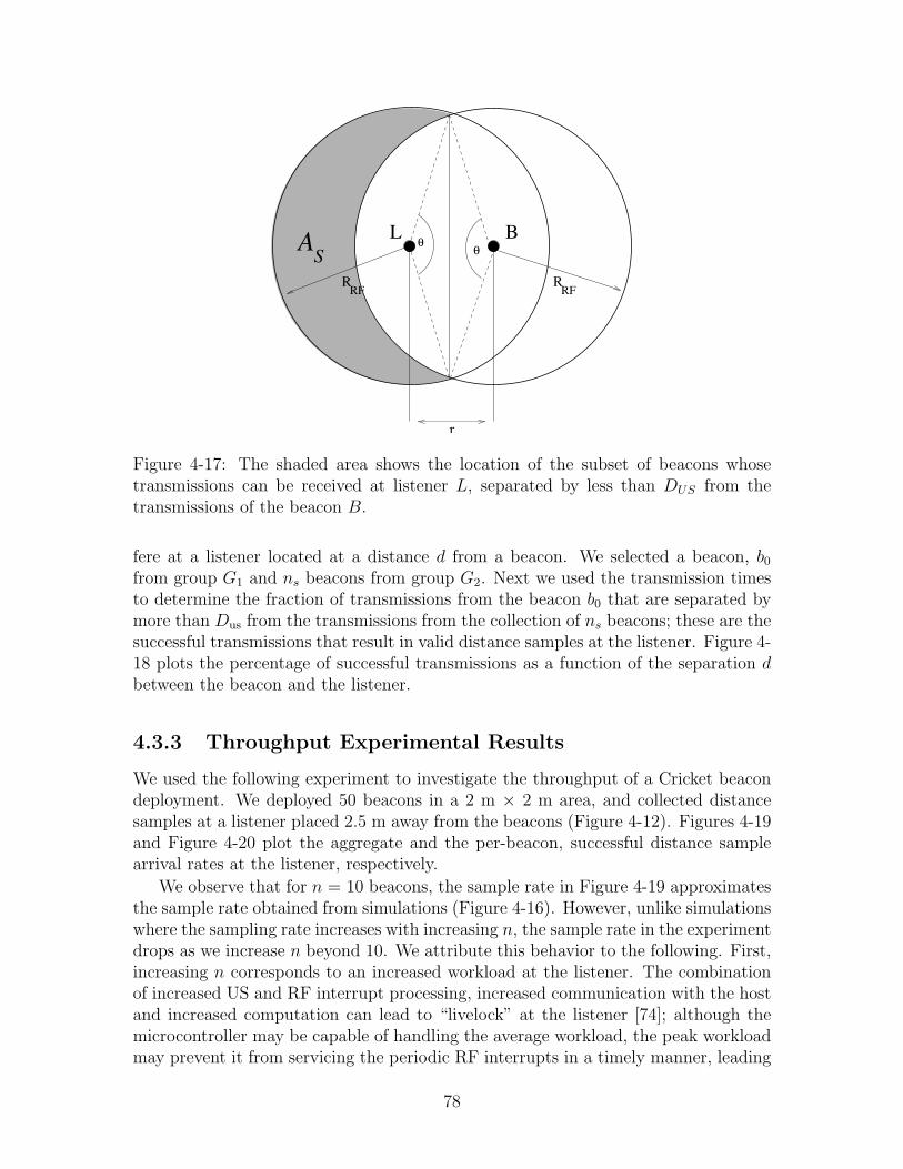
4-17 The shaded area shows the location of the subset of beacons whosetransmissions can be received at listener L, separated by less thanDUS from the transmissions of the beacon B. . . . . . . . . . . . . . . 78
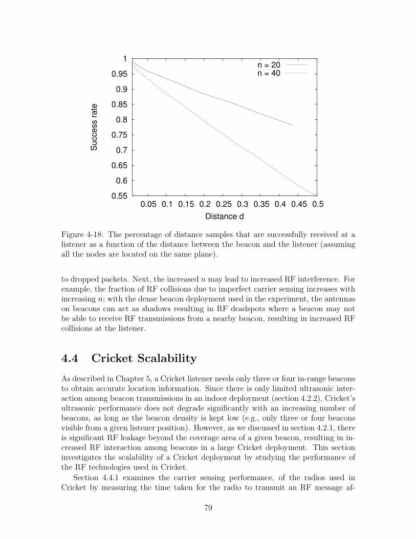
4-18 The percentage of distance samples that are successfully received ata listener as a function of the distance between the beacon and thelistener (assuming all the nodes are located on the same plane). . . . 79
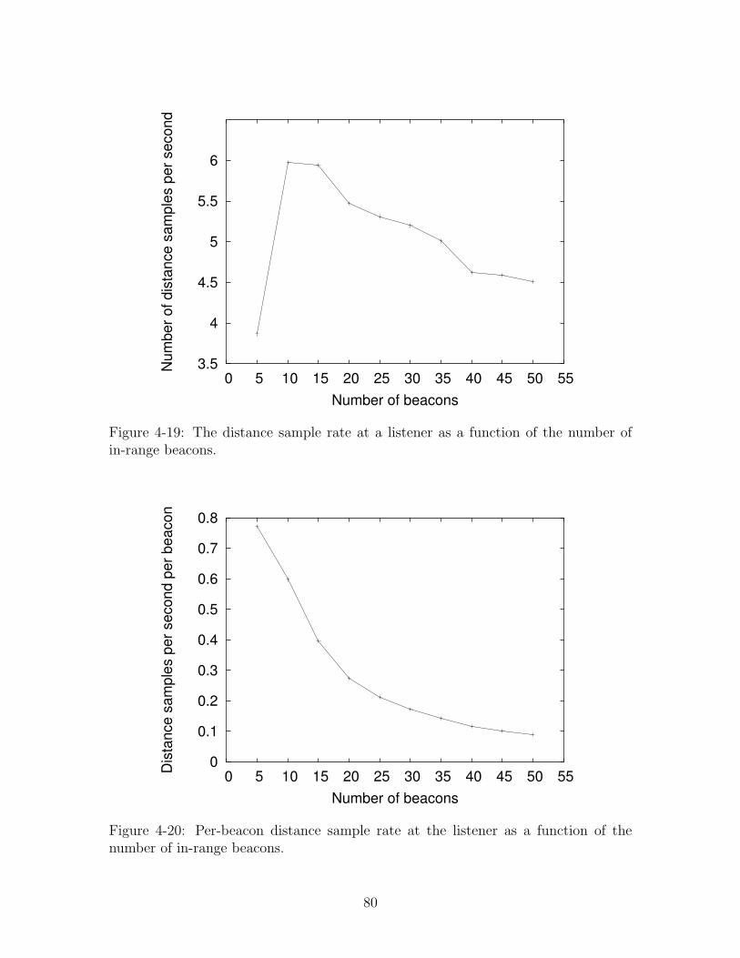
4-19 The distance sample rate at a listener as a function of the number ofin-range beacons. . . . . . . . . . . . . . . . . . . . . . . . . . . . . . 80
4-20 Per-beacon distance sample rate at the listener as a function of thenumber of in-range beacons. . . . . . . . . . . . . . . . . . . . . . . . 80
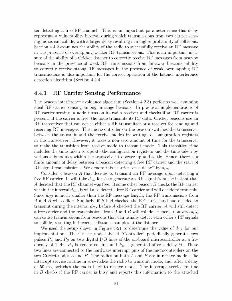
4-21 Experimental setup to determine the carrier sensing delay, dCS. Thecontroller generates two pulses PA and PB separated by a delay δt.When PA arrives, node A starts its RF transmitter; when PB arrives,node B checks the RF carrier status and reports it to the attachedhost, which logs this data. . . . . . . . . . . . . . . . . . . . . . . . . 82
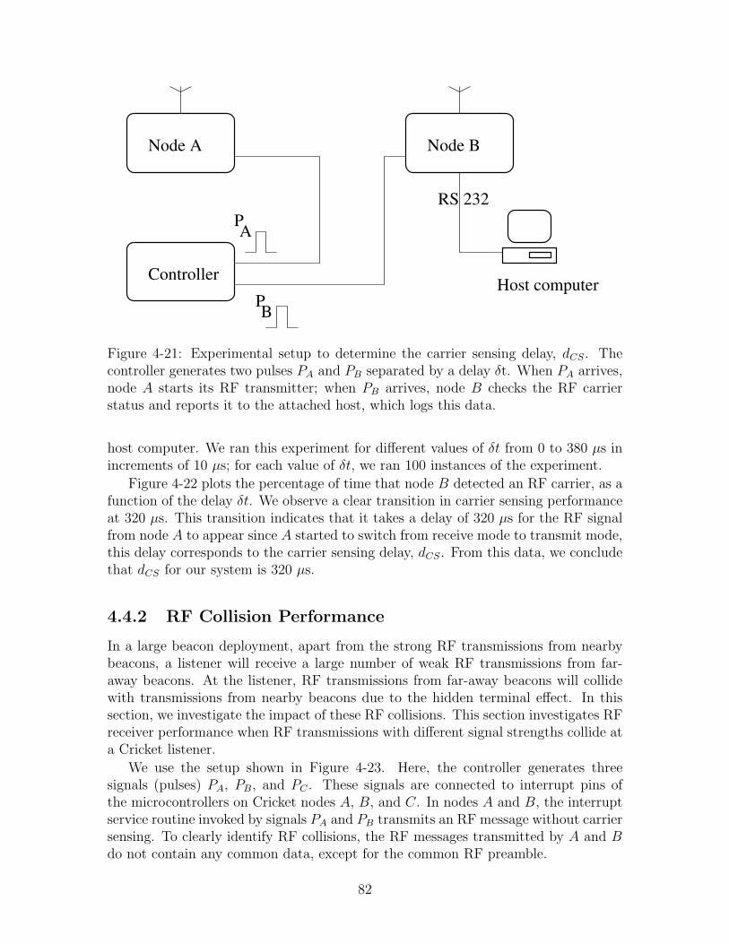
4-22 The percentage of time the RF carrier is detected by node B as afunction of the delay between node A starting its RF transmitter andnode B sensing for RF carrier. . . . . . . . . . . . . . . . . . . . . . . 83
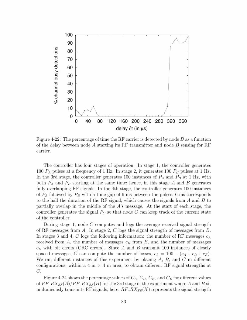
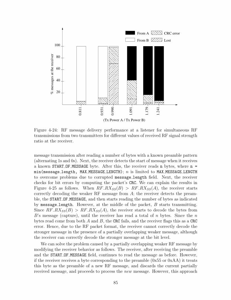
4-24 RF message delivery performance at a listener for simultaneous RFtransmissions from two transmitters for different values of received RFsignal strength ratio at the receiver. . . . . . . . . . . . . . . . . . . . 85
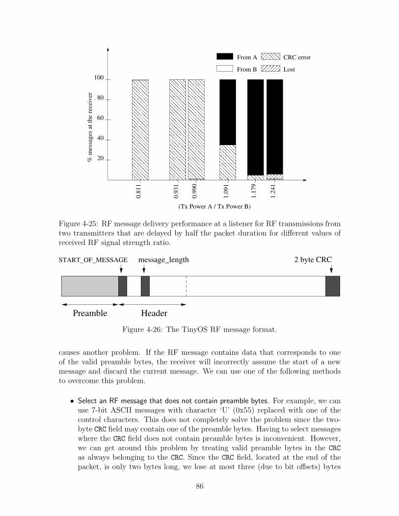
4-25 RF message delivery performance at a listener for RF transmissionsfrom two transmitters that are delayed by half the packet duration fordifferent values of received RF signal strength ratio. . . . . . . . . . . 86
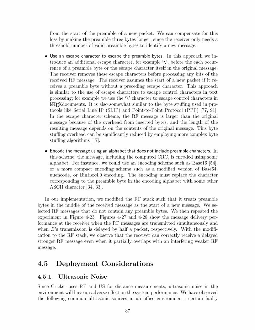
4-27 RF message delivery performance at a listener for simultaneous RFtransmissions from two transmitters for different values of received RFsignal strength ratio with the receiver starting a new packet upon thereceipt of preamble bytes. . . . . . . . . . . . . . . . . . . . . . . . . 88
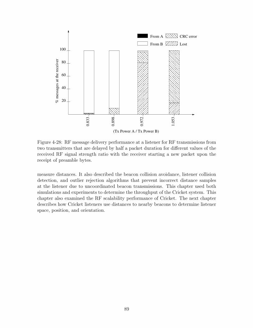
4-28 RF message delivery performance at a listener for RF transmissionsfrom two transmitters that are delayed by half a packet duration fordifferent values of the received RF signal strength ratio with the re-ceiver starting a new packet upon the receipt of preamble bytes. . . . 89
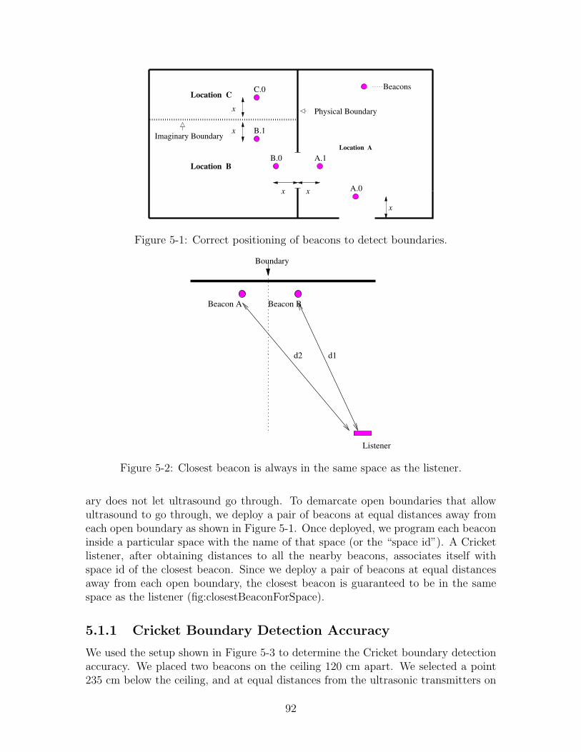
5-1 Correct positioning of beacons to detect boundaries. . . . . . . . . . . 92
5-2 Closest beacon is always in the same space as the listener. . . . . . . 92
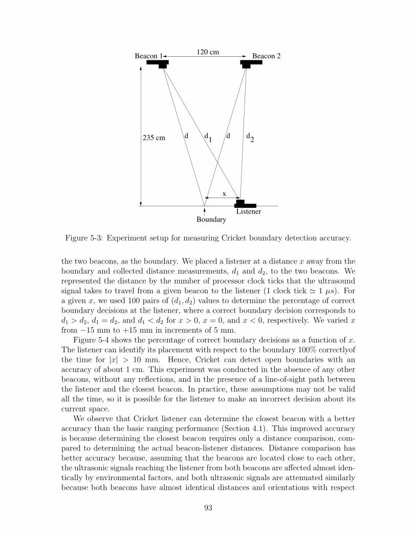
5-3 Experiment setup for measuring Cricket boundary detection accuracy. 93
15
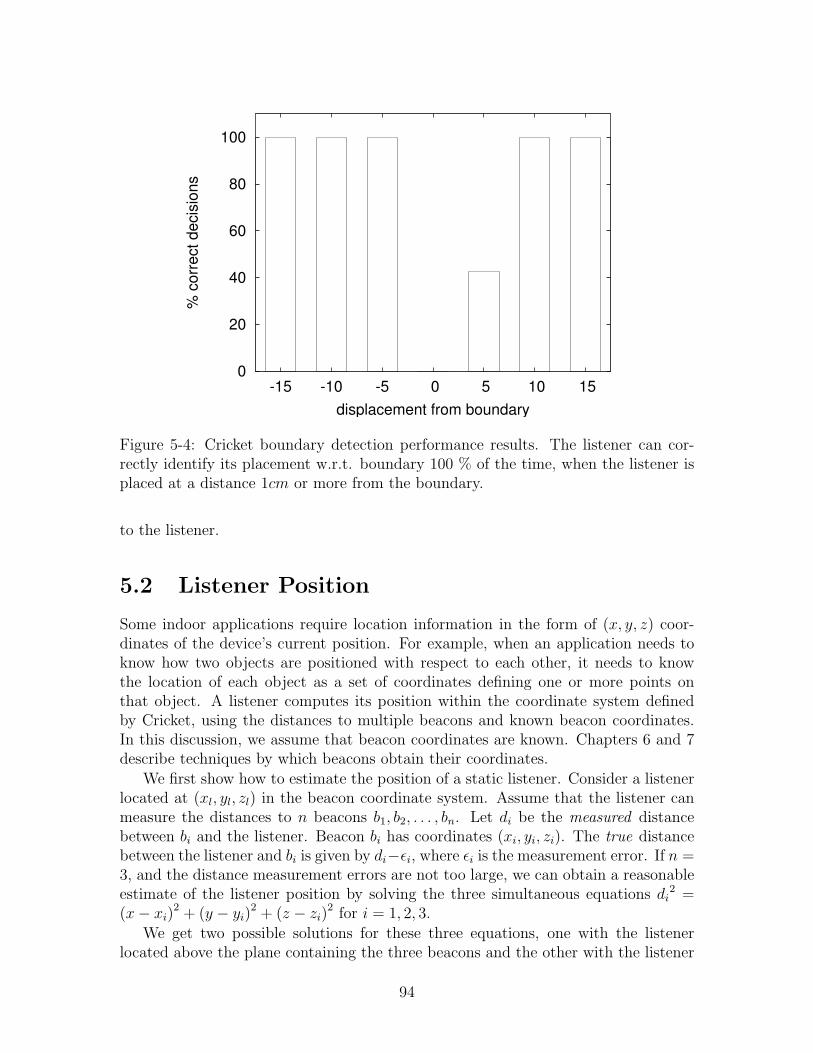
5-4 Cricket boundary detection performance results. The listener can cor-rectly identify its placement w.r.t. boundary 100 % of the time, whenthe listener is placed at a distance 1cm or more from the boundary. . 94
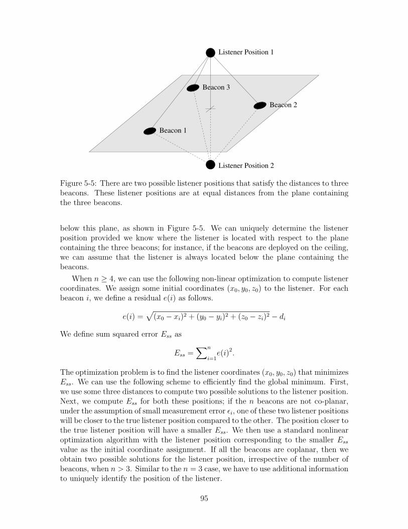
5-5 There are two possible listener positions that satisfy the distances tothree beacons. These listener positions are at equal distances from theplane containing the three beacons. . . . . . . . . . . . . . . . . . . . 95
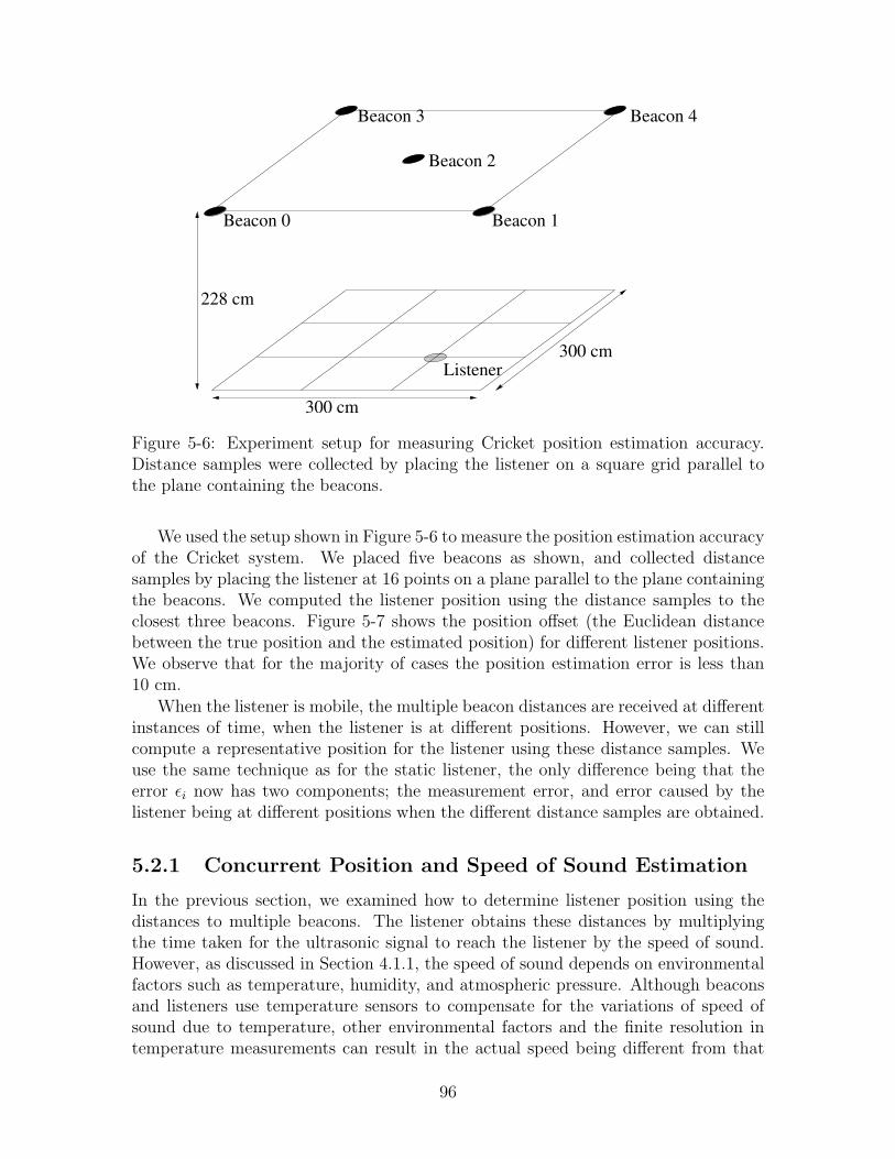
5-6 Experiment setup for measuring Cricket position estimation accuracy.Distance samples were collected by placing the listener on a square gridparallel to the plane containing the beacons. . . . . . . . . . . . . . . 96
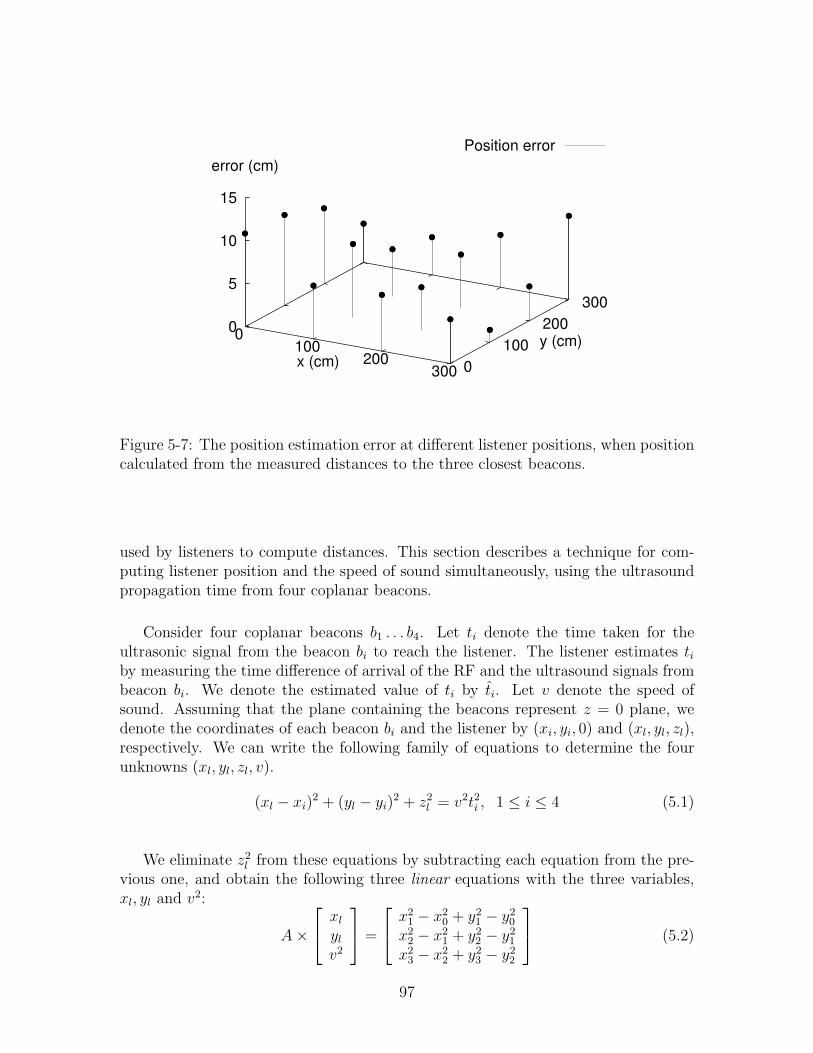
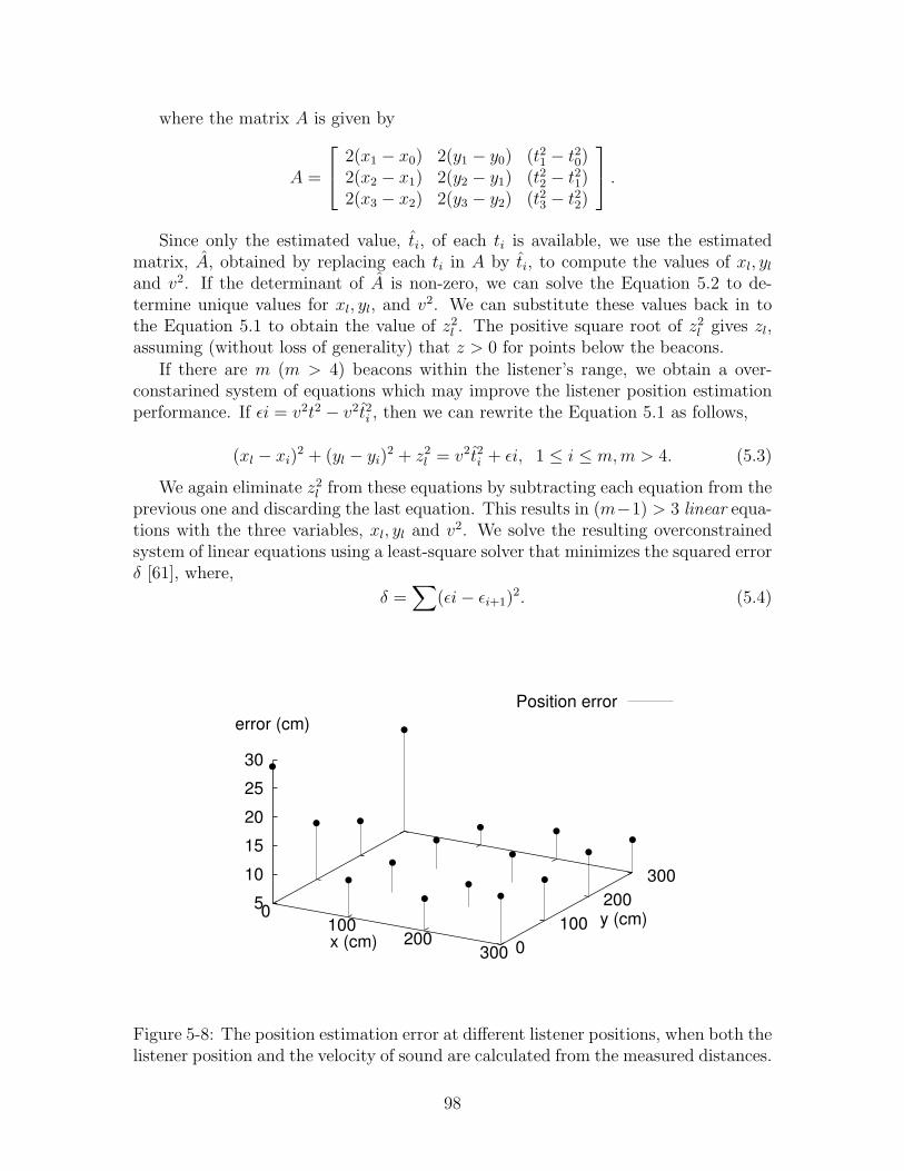
5-7 The position estimation error at different listener positions, when posi-tion calculated from the measured distances to the three closest beacons. 97
5-8 The position estimation error at different listener positions, when boththe listener position and the velocity of sound are calculated from themeasured distances. . . . . . . . . . . . . . . . . . . . . . . . . . . . . 98
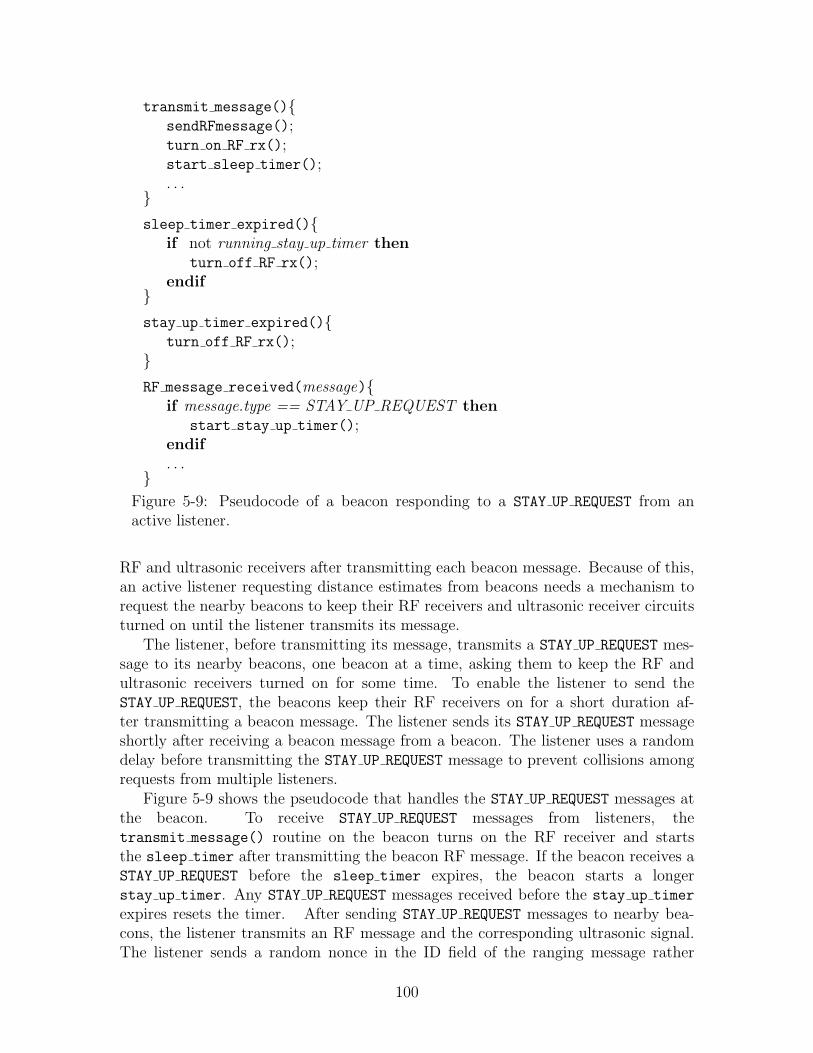
5-9 Pseudocode of a beacon responding to a STAY UP REQUEST from anactive listener. . . . . . . . . . . . . . . . . . . . . . . . . . . . . . . . 100
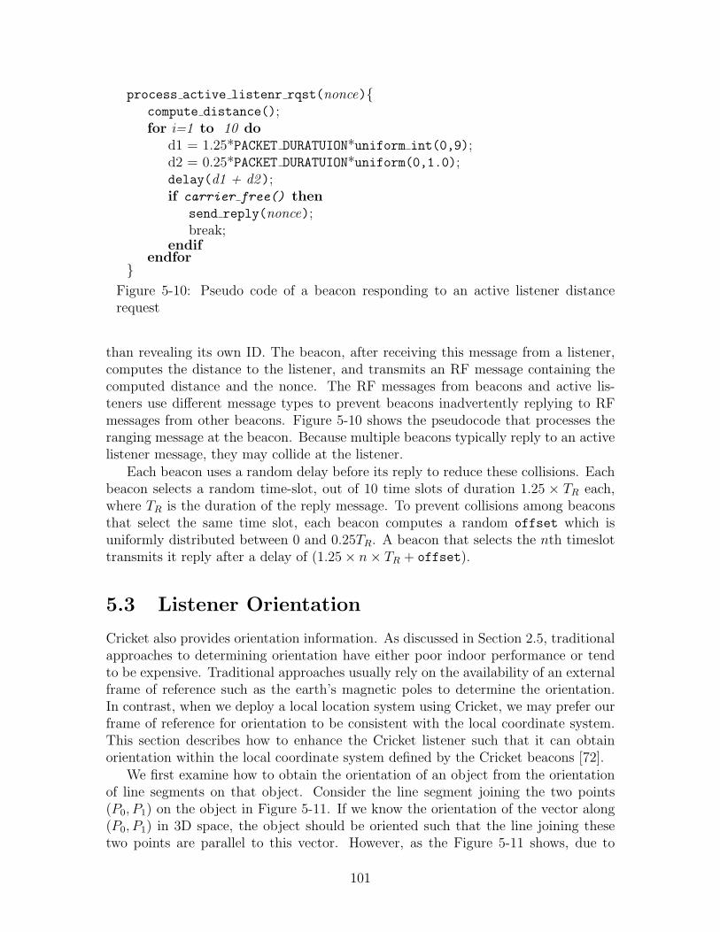
5-10 Pseudo code of a beacon responding to an active listener distance request101
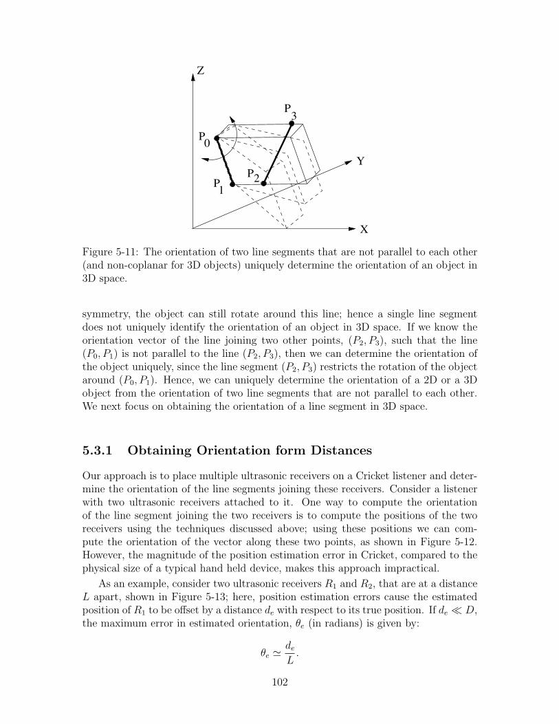
5-11 The orientation of two line segments that are not parallel to each other(and non-coplanar for 3D objects) uniquely determine the orientationof an object in 3D space. . . . . . . . . . . . . . . . . . . . . . . . . . 102
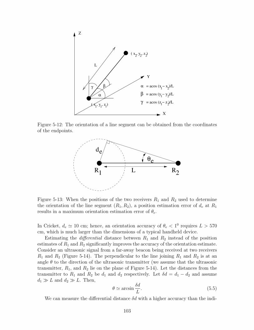
5-12 The orientation of a line segment can be obtained from the coordinatesof the endpoints. . . . . . . . . . . . . . . . . . . . . . . . . . . . . . 103
5-13 When the positions of the two receivers R1 and R2 used to determinethe orientation of the line segment (R1, R2), a position estimation errorof de at R1 results in a maximum orientation estimation error of θe. . 103
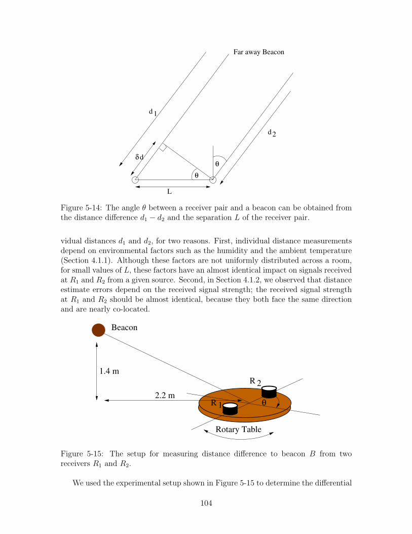
5-14 The angle θ between a receiver pair and a beacon can be obtained fromthe distance difference d1 − d2 and the separation L of the receiver pair.104
5-15 The setup for measuring distance difference to beacon B from tworeceivers R1 and R2. . . . . . . . . . . . . . . . . . . . . . . . . . . . 104
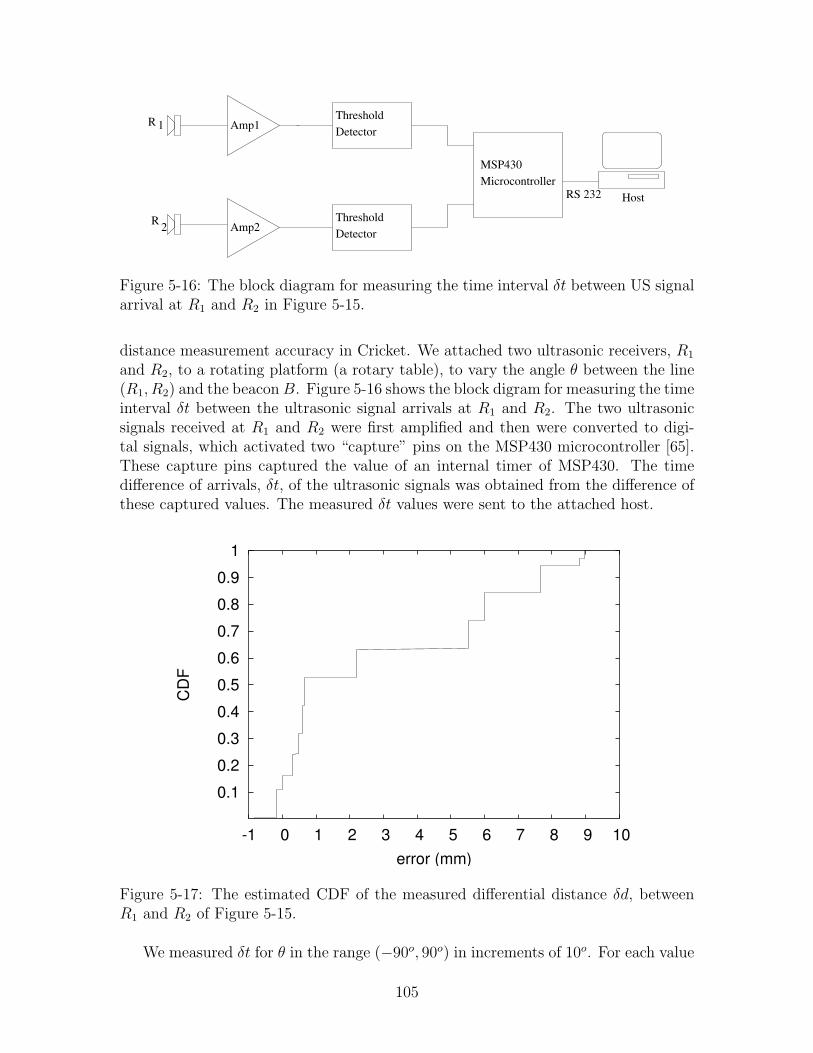
5-16 The block diagram for measuring the time interval δt between US signalarrival at R1 and R2 in Figure 5-15. . . . . . . . . . . . . . . . . . . . 105
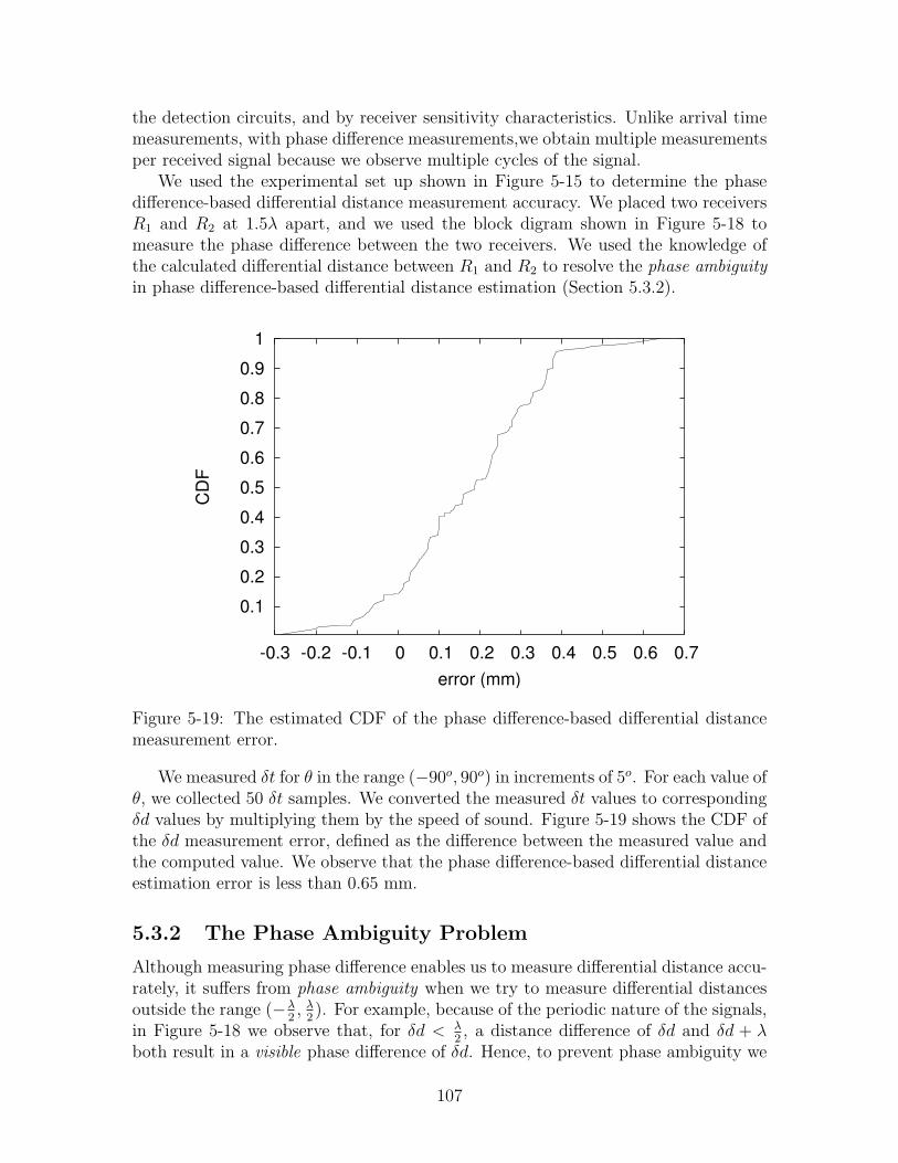
5-17 The estimated CDF of the measured differential distance δd, betweenR1 and R2 of Figure 5-15. . . . . . . . . . . . . . . . . . . . . . . . . 105
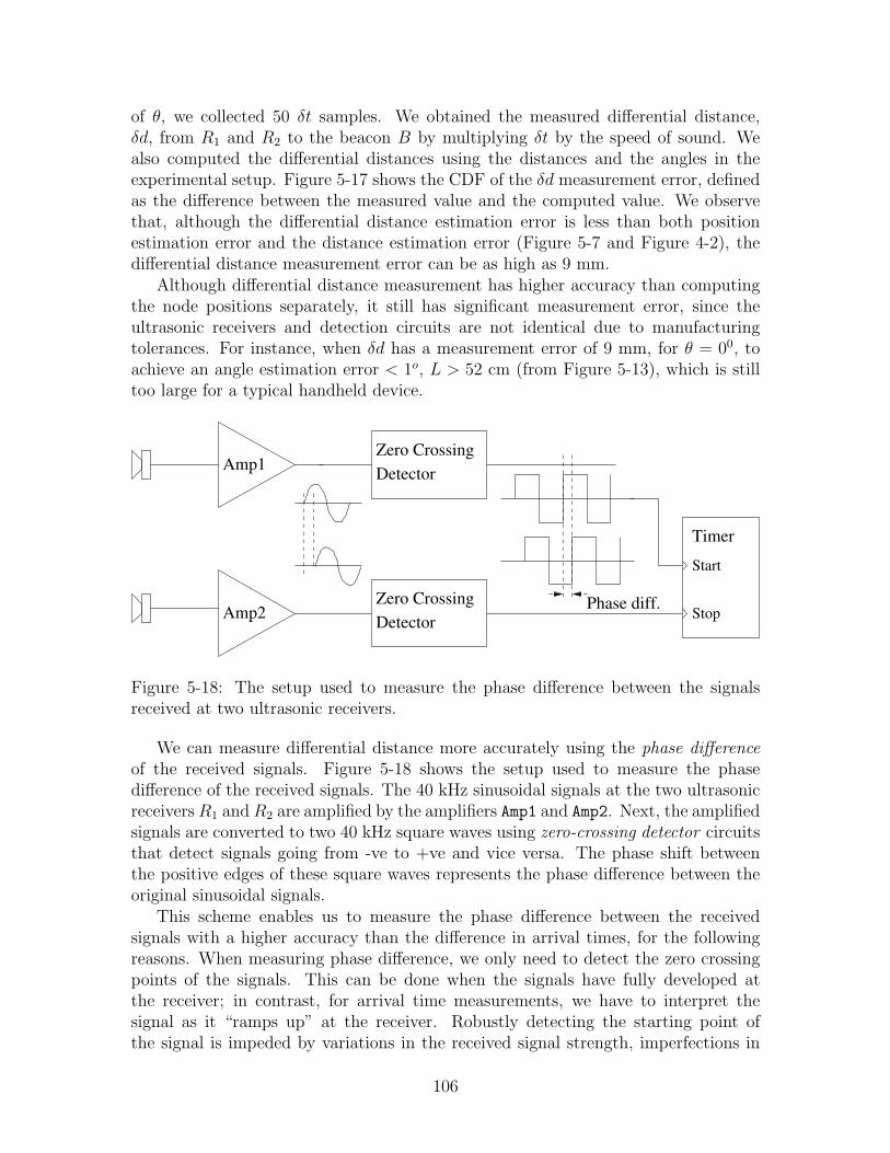
5-18 The setup used to measure the phase difference between the signalsreceived at two ultrasonic receivers. . . . . . . . . . . . . . . . . . . . 106
5-20 Using three receivers to measure (d1 − d2). . . . . . . . . . . . . . . . 109
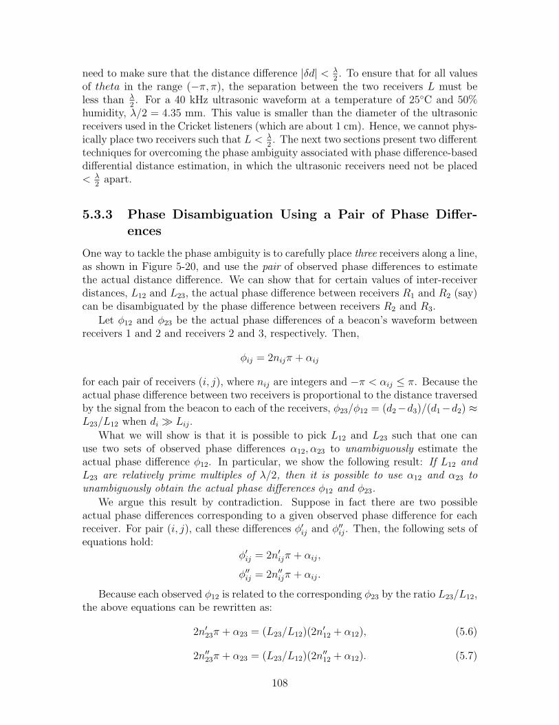
5-21 Finding the actual differential distance between R1 and R2 by usingthe observed differential distances from (R1, R2) and (R2, R3). . . . . 110
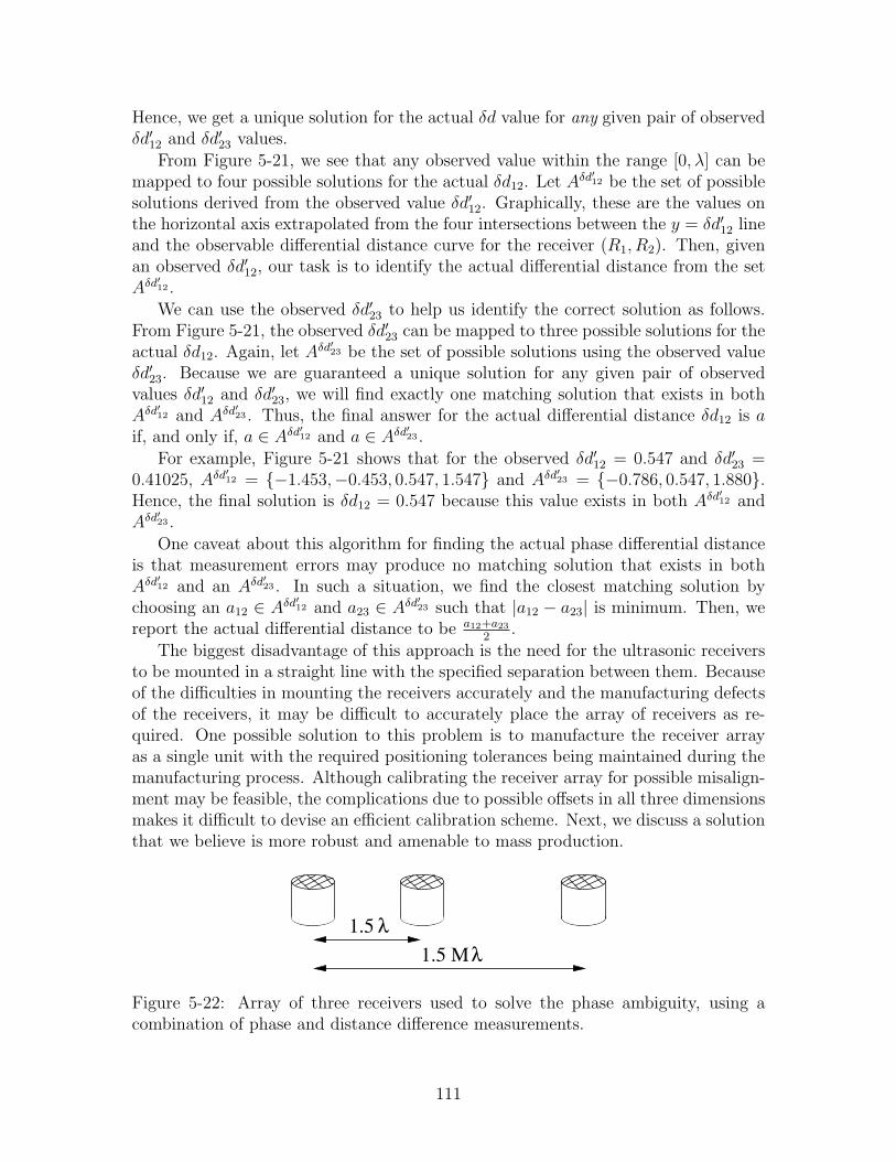
5-22 Array of three receivers used to solve the phase ambiguity, using acombination of phase and distance difference measurements. . . . . . 111
16
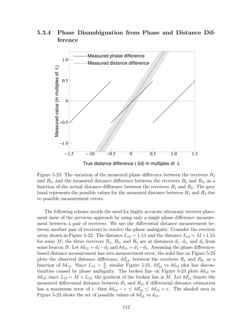
5-23 The variation of the measured phase difference between the receiversR1 and R2, and the measured distance difference between the receiversR1 and R3, as a function of the actual distance difference between thereceivers R1 and R2. The grey band represents the possible values forthe measured distance between R1 and R3 due to possible measurementerrors. . . . . . . . . . . . . . . . . . . . . . . . . . . . . . . . . . . . 112
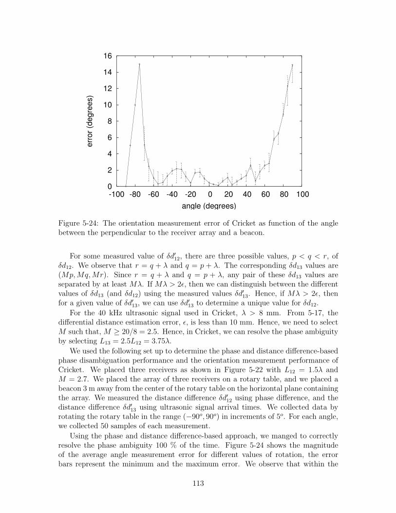
5-24 The orientation measurement error of Cricket as function of the anglebetween the perpendicular to the receiver array and a beacon. . . . . 113
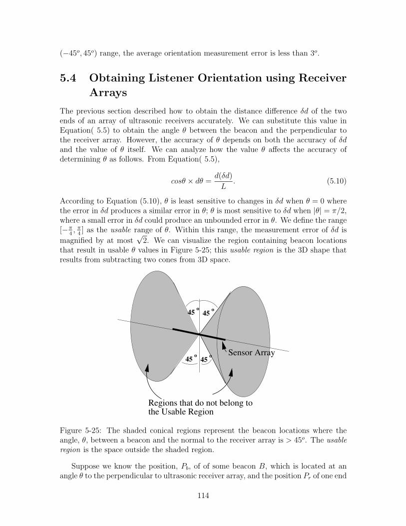
5-25 The shaded conical regions represent the beacon locations where theangle, θ, between a beacon and the normal to the receiver array is> 45o. The usable region is the space outside the shaded region. . . . 114
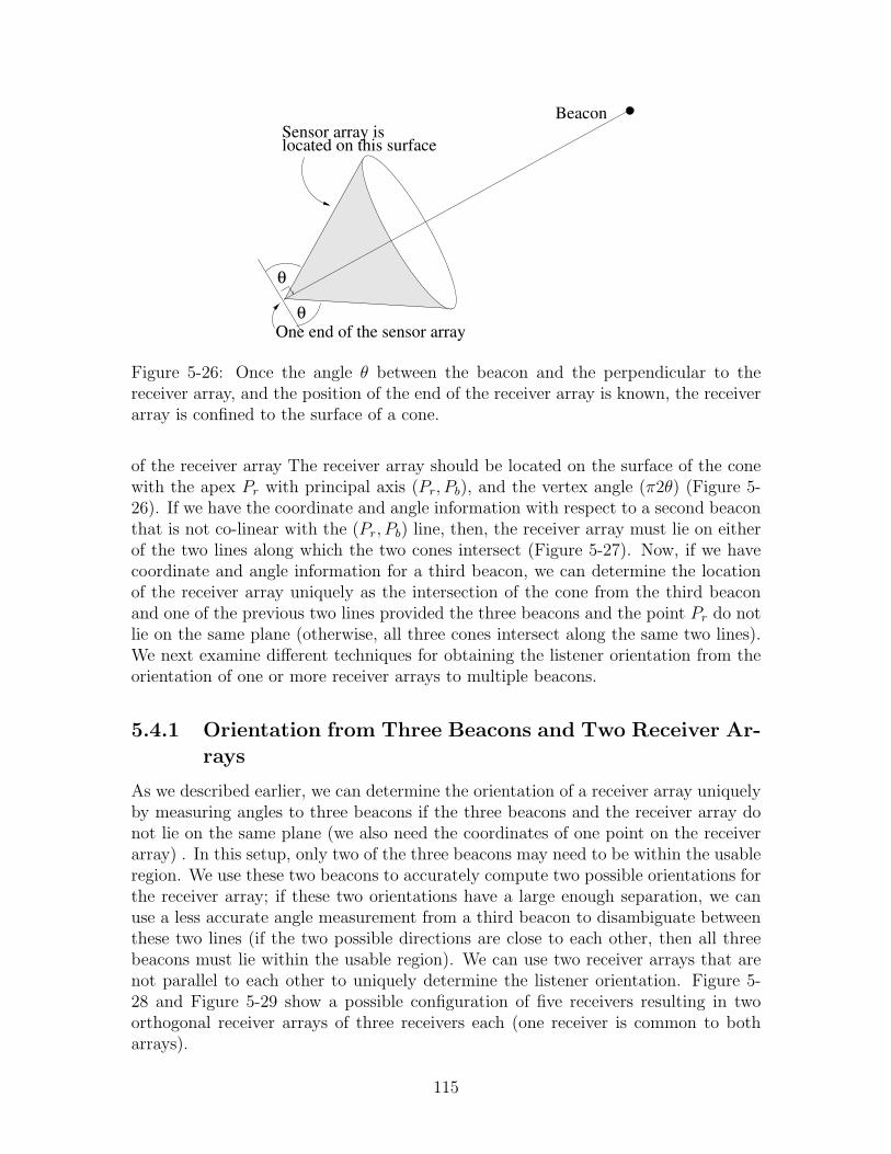
5-26 Once the angle θ between the beacon and the perpendicular to thereceiver array, and the position of the end of the receiver array is known,the receiver array is confined to the surface of a cone. . . . . . . . . . 115
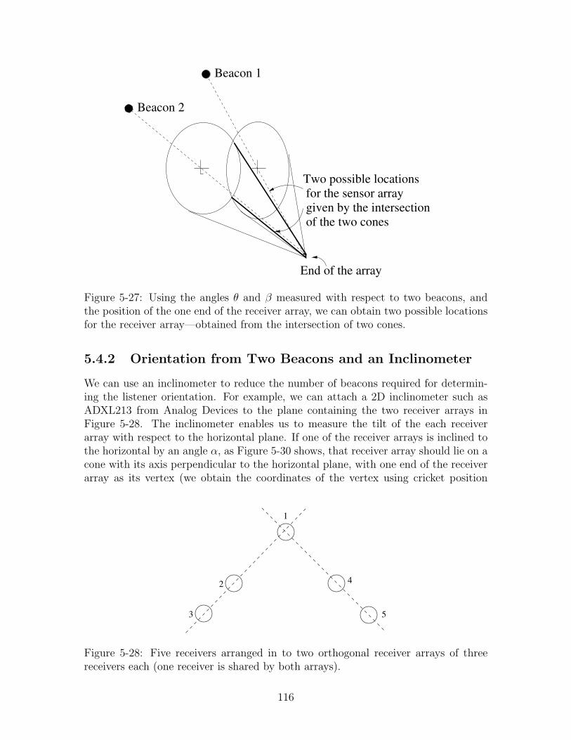
5-27 Using the angles θ and β measured with respect to two beacons, and theposition of the one end of the receiver array, we can obtain two possiblelocations for the receiver array—obtained from the intersection of twocones. . . . . . . . . . . . . . . . . . . . . . . . . . . . . . . . . . . . 116
5-28 Five receivers arranged in to two orthogonal receiver arrays of threereceivers each (one receiver is shared by both arrays). . . . . . . . . . 116
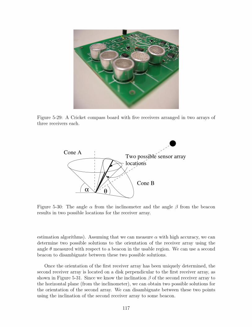
5-29 A Cricket compass board with five receivers arranged in two arrays ofthree receivers each. . . . . . . . . . . . . . . . . . . . . . . . . . . . . 117
5-30 The angle α from the inclinometer and the angle β from the beaconresults in two possible locations for the receiver array. . . . . . . . . . 117
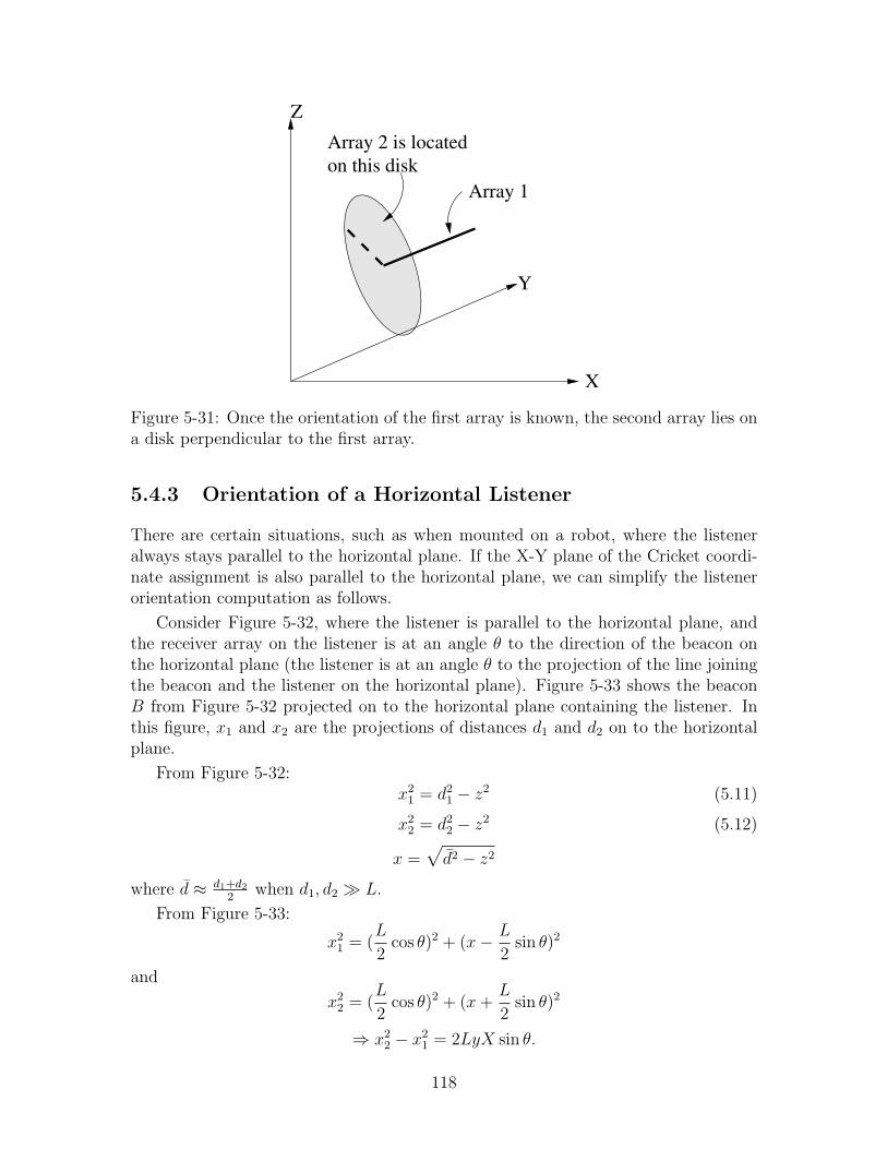
5-31 Once the orientation of the first array is known, the second array lieson a disk perpendicular to the first array. . . . . . . . . . . . . . . . . 118
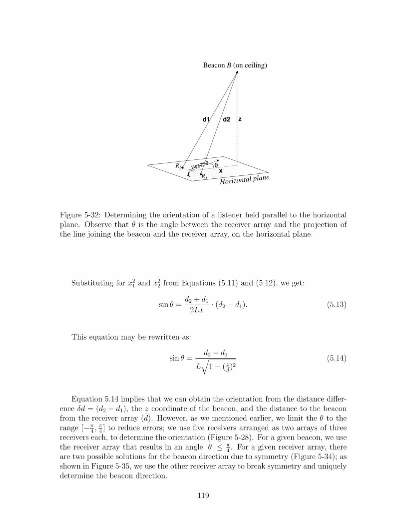
5-32 Determining the orientation of a listener held parallel to the horizontalplane. Observe that θ is the angle between the receiver array and theprojection of the line joining the beacon and the receiver array, on thehorizontal plane. . . . . . . . . . . . . . . . . . . . . . . . . . . . . . 119
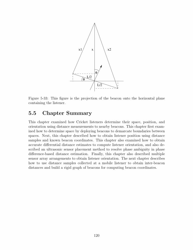
5-33 This figure is the projection of the beacon onto the horizontal planecontaining the listener. . . . . . . . . . . . . . . . . . . . . . . . . . . 120
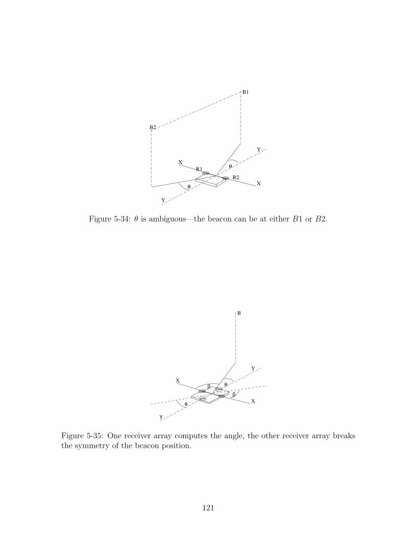
5-34 θ is ambiguous—the beacon can be at either B1 or B2. . . . . . . . . 121
5-35 One receiver array computes the angle, the other receiver array breaksthe symmetry of the beacon position. . . . . . . . . . . . . . . . . . . 121
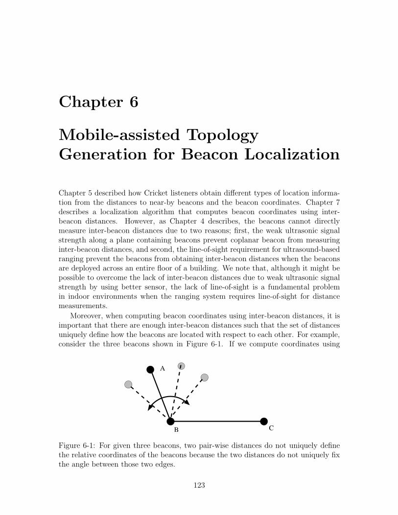
6-1 For given three beacons, two pair-wise distances do not uniquely definethe relative coordinates of the beacons because the two distances donot uniquely fix the angle between those two edges. . . . . . . . . . . 123
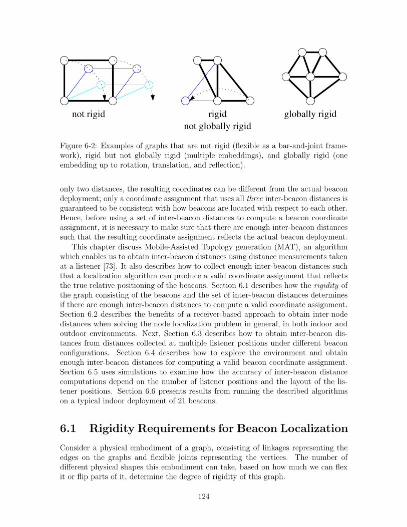
6-2 Examples of graphs that are not rigid (flexible as a bar-and-joint frame-work), rigid but not globally rigid (multiple embeddings), and globallyrigid (one embedding up to rotation, translation, and reflection). . . . 124
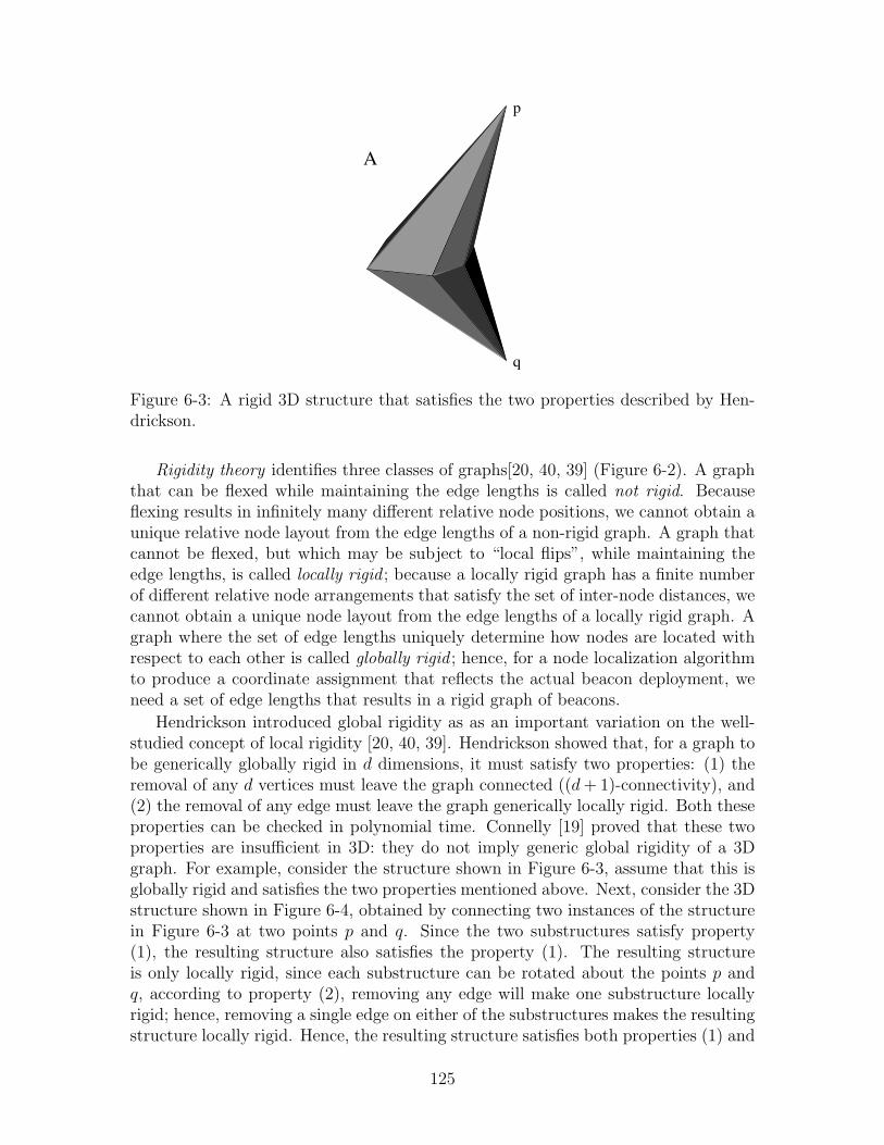
6-3 A rigid 3D structure that satisfies the two properties described byHendrickson. . . . . . . . . . . . . . . . . . . . . . . . . . . . . . . . . 125
17
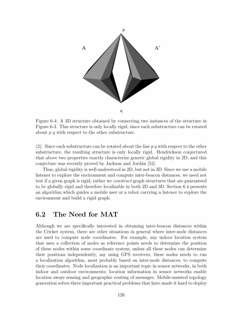
6-4 A 3D structure obtained by connecting two instances of the structure inFigure 6-3. This structure is only locally rigid, since each substructurecan be rotated about p q with respect to the other substructure. . . . 126
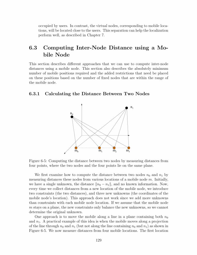
6-5 Computing the distance between two nodes by measuring distancesfrom four points, where the two nodes and the four points lie on thesame plane. . . . . . . . . . . . . . . . . . . . . . . . . . . . . . . . . 129
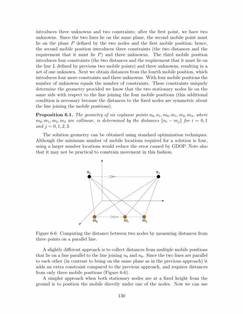
6-6 Computing the distance between two nodes by measuring distancesfrom three points on a parallel line. . . . . . . . . . . . . . . . . . . . 130
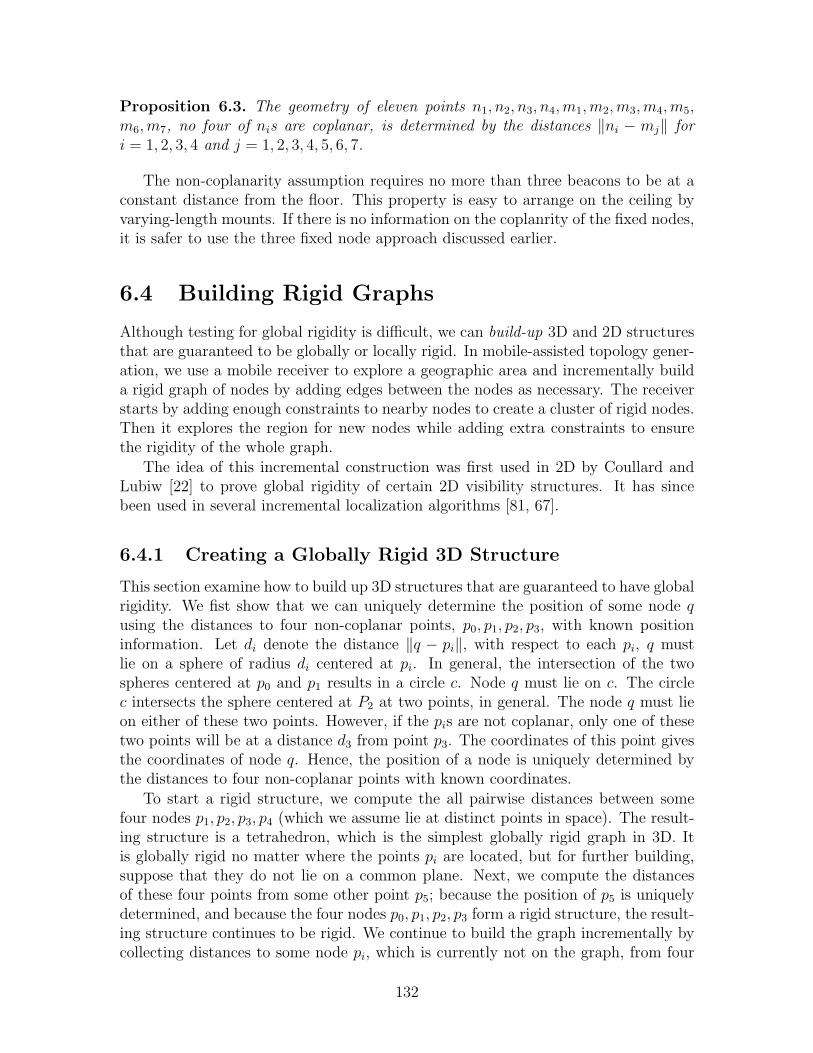
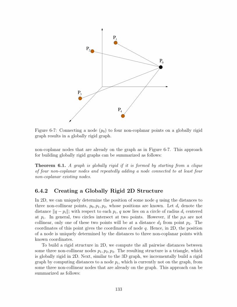
6-7 Connecting a node (p0) to four non-coplanar points on a globally rigidgraph results in a globally rigid graph. . . . . . . . . . . . . . . . . . 133
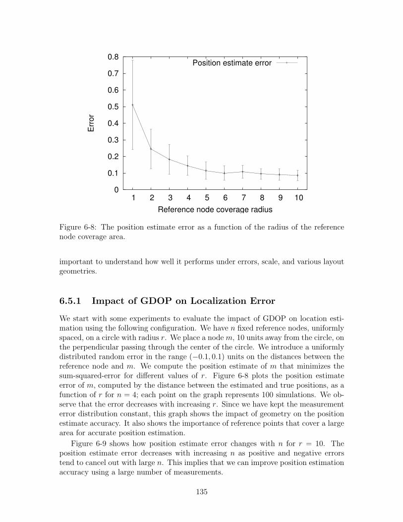
6-8 The position estimate error as a function of the radius of the referencenode coverage area. . . . . . . . . . . . . . . . . . . . . . . . . . . . . 135
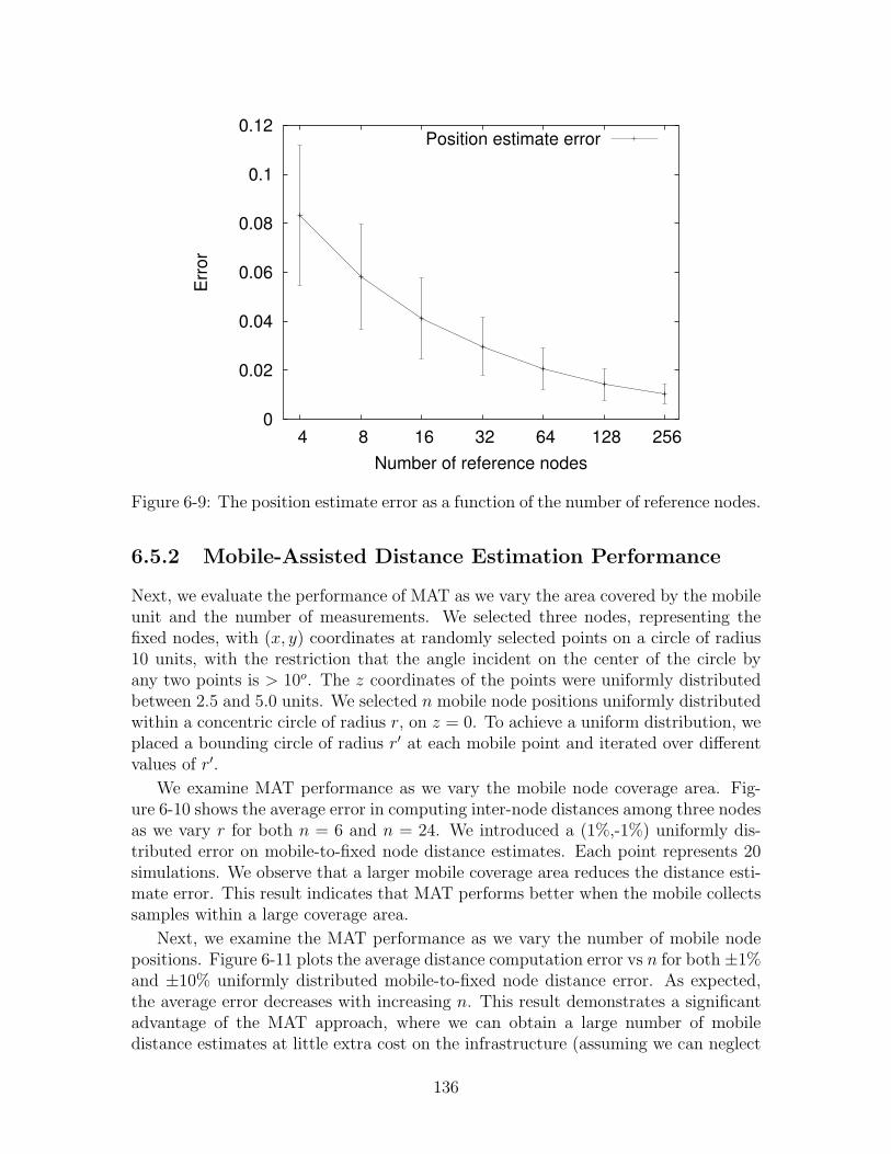
6-9 The position estimate error as a function of the number of referencenodes. . . . . . . . . . . . . . . . . . . . . . . . . . . . . . . . . . . . 136
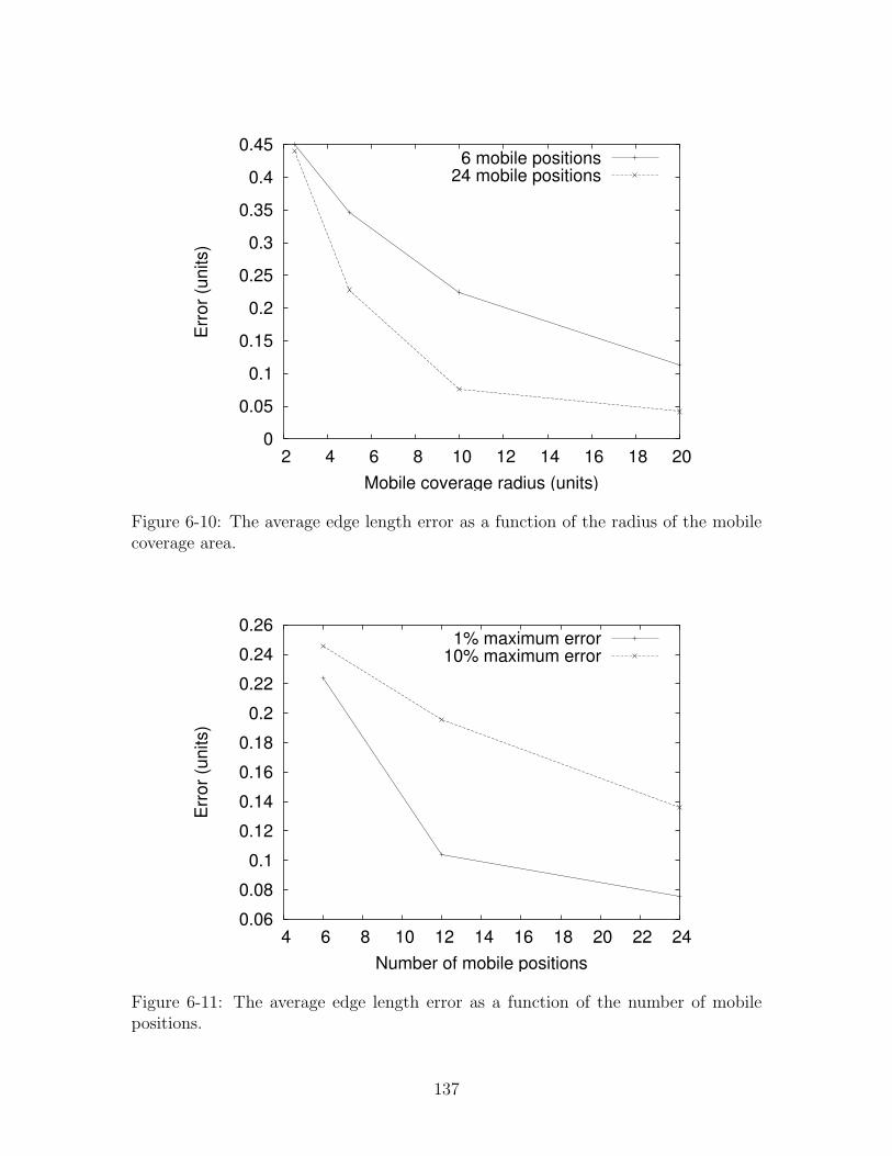
6-10 The average edge length error as a function of the radius of the mobilecoverage area. . . . . . . . . . . . . . . . . . . . . . . . . . . . . . . . 137
6-11 The average edge length error as a function of the number of mobilepositions. . . . . . . . . . . . . . . . . . . . . . . . . . . . . . . . . . 137
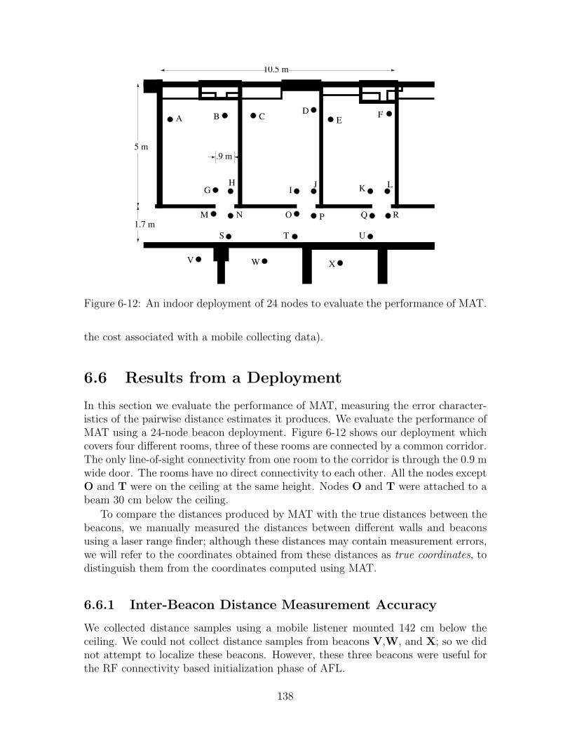
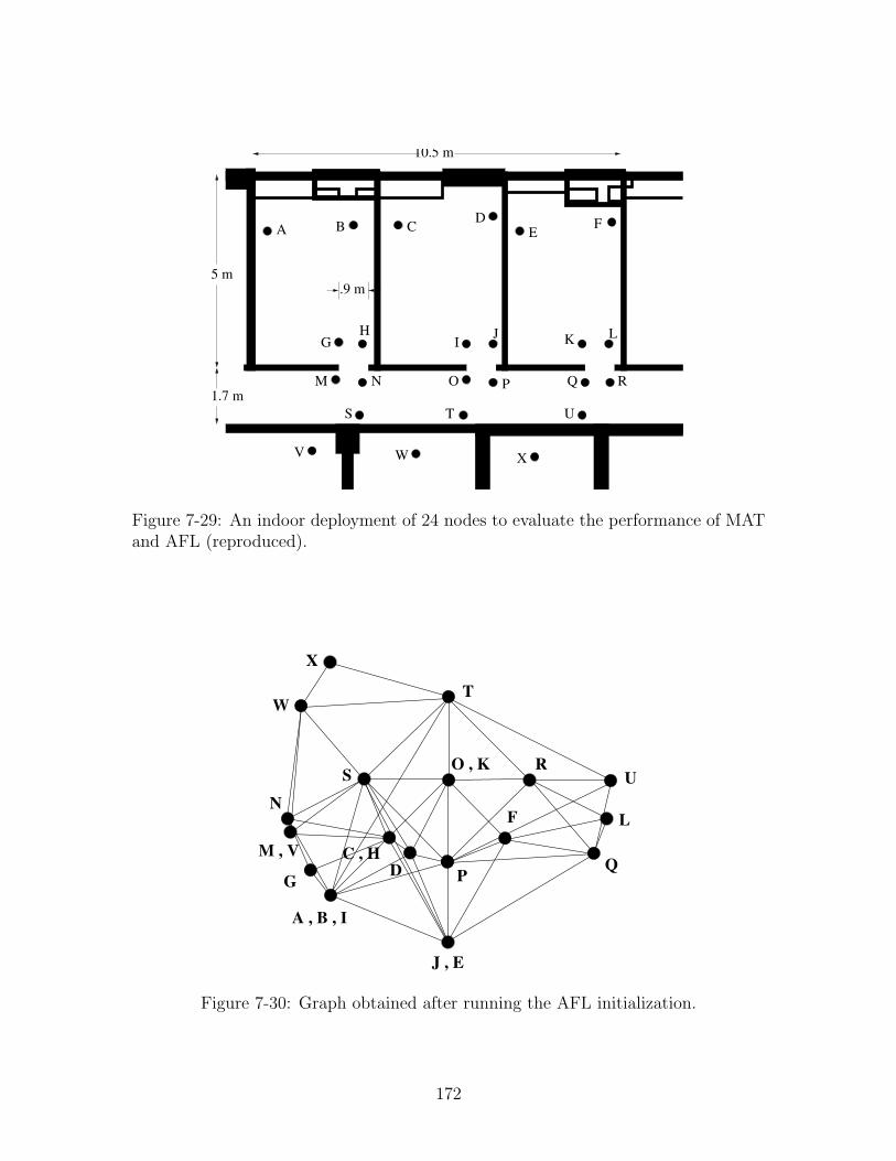
6-12 An indoor deployment of 24 nodes to evaluate the performance of MAT.138
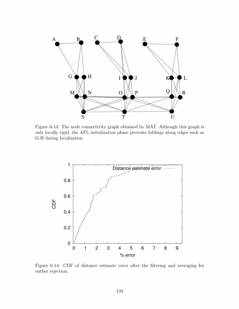
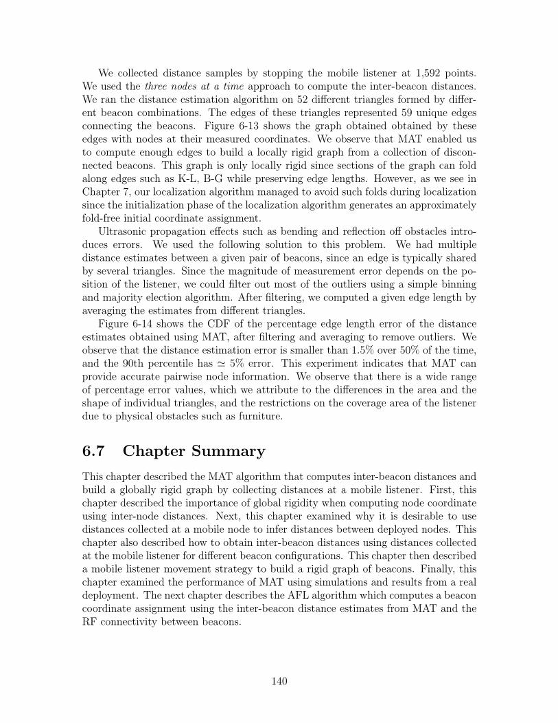
6-13 The node connectivity graph obtained by MAT. Although this graph isonly locally rigid, the AFL initialization phase prevents foldings alongedges such as G-H during localization. . . . . . . . . . . . . . . . . . 139
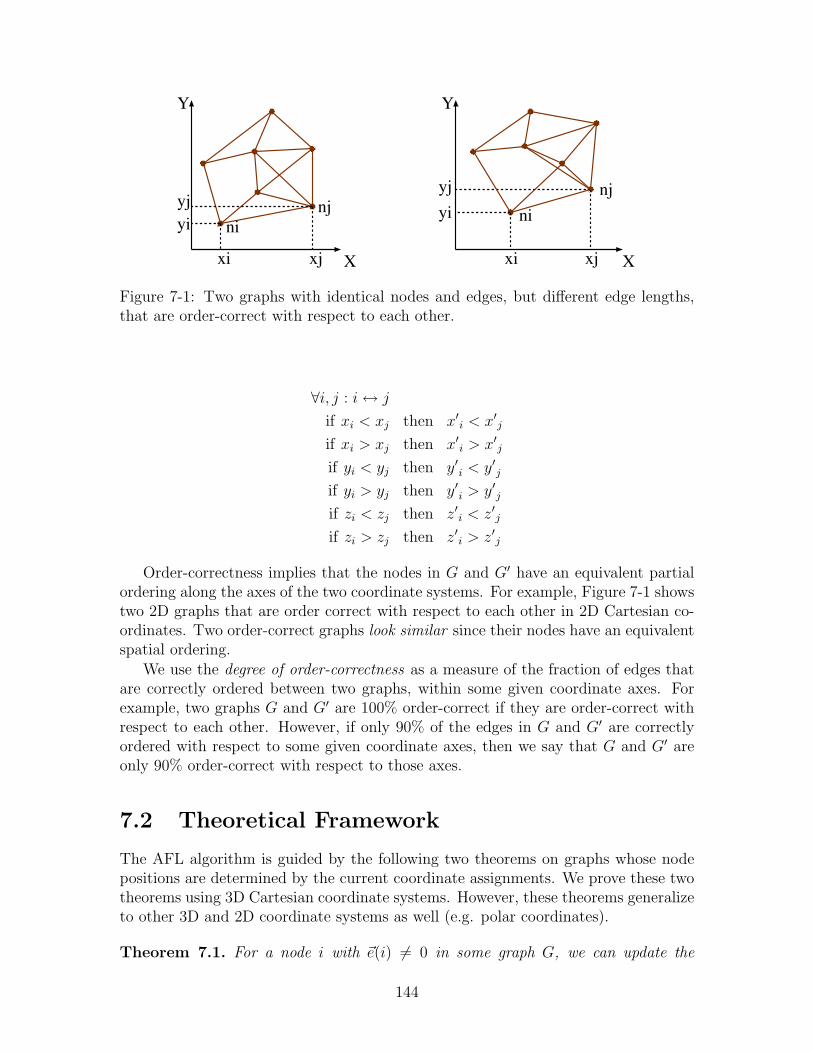
7-1 Two graphs with identical nodes and edges, but different edge lengths,that are order-correct with respect to each other. . . . . . . . . . . . 144
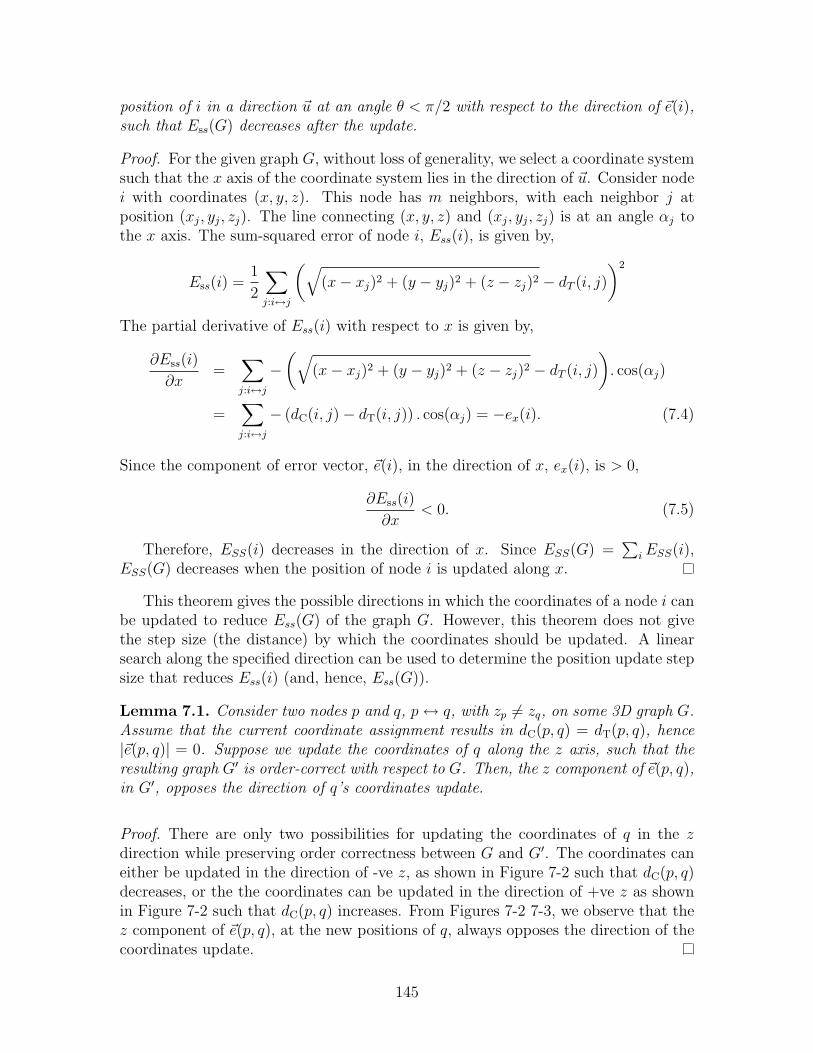
7-2 When node q’s coordinates are updated in -ve z, ~e(p, q) has a +ve zcomponent. . . . . . . . . . . . . . . . . . . . . . . . . . . . . . . . . 146
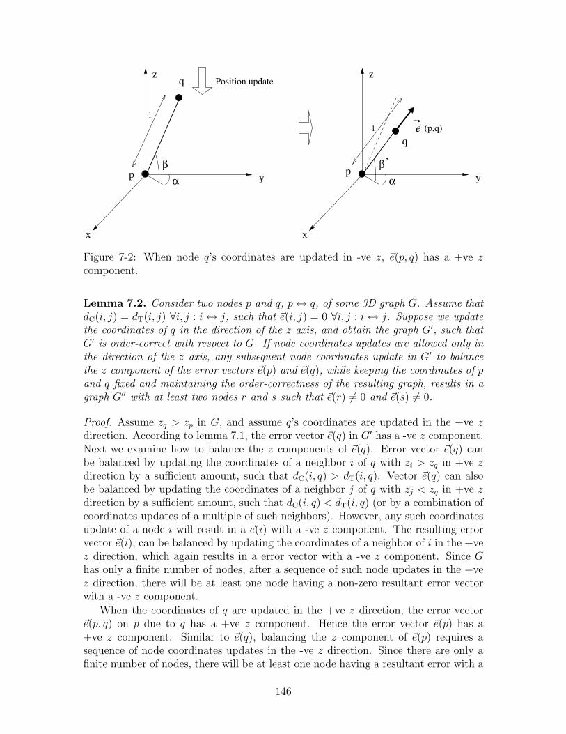
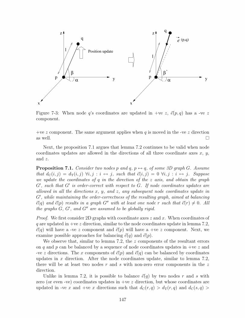
7-3 When node q’s coordinates are updated in +ve z, ~e(p, q) has a -ve zcomponent. . . . . . . . . . . . . . . . . . . . . . . . . . . . . . . . . 147
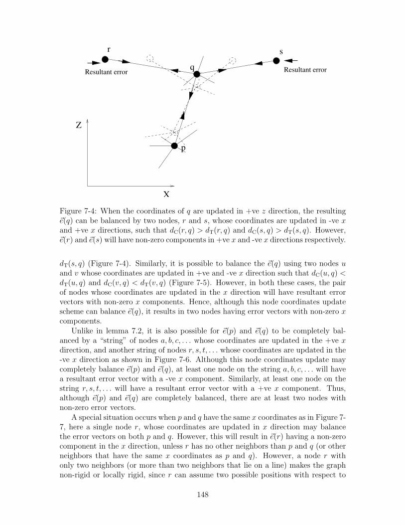
7-4 When the coordinates of q are updated in +ve z direction, the resulting~e(q) can be balanced by two nodes, r and s, whose coordinates areupdated in -ve x and +ve x directions, such that dC(r, q) > dT(r, q)and dC(s, q) > dT(s, q). However, ~e(r) and ~e(s) will have non-zerocomponents in +ve x and -ve x directions respectively. . . . . . . . . 148
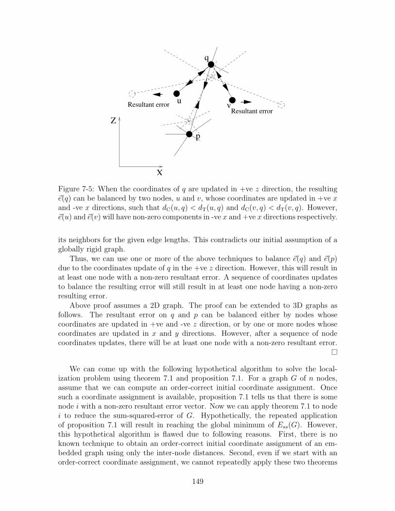
7-5 When the coordinates of q are updated in +ve z direction, the resulting~e(q) can be balanced by two nodes, u and v, whose coordinates areupdated in +ve x and -ve x directions, such that dC(u, q) < dT(u, q)and dC(v, q) < dT(v, q). However, ~e(u) and ~e(v) will have non-zerocomponents in -ve x and +ve x directions respectively. . . . . . . . . 149
18
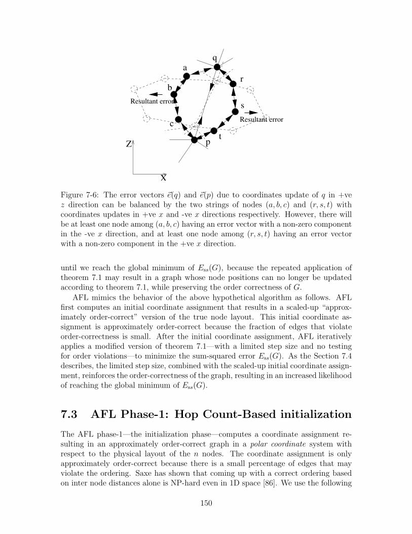
7-6 The error vectors ~e(q) and ~e(p) due to coordinates update of q in +vez direction can be balanced by the two strings of nodes (a, b, c) and(r, s, t) with coordinates updates in +ve x and -ve x directions respec-tively. However, there will be at least one node among (a, b, c) havingan error vector with a non-zero component in the -ve x direction, andat least one node among (r, s, t) having an error vector with a non-zerocomponent in the +ve x direction. . . . . . . . . . . . . . . . . . . . . 150
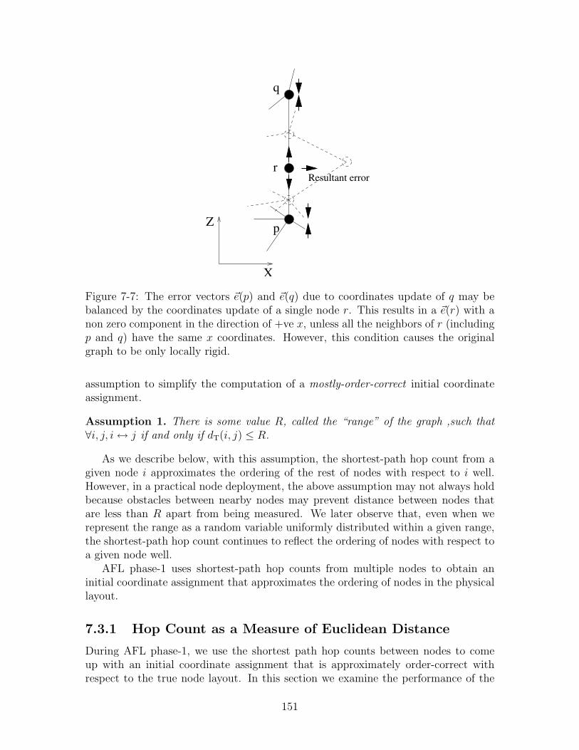
7-7 The error vectors ~e(p) and ~e(q) due to coordinates update of q may bebalanced by the coordinates update of a single node r. This results ina ~e(r) with a non zero component in the direction of +ve x, unless allthe neighbors of r (including p and q) have the same x coordinates.However, this condition causes the original graph to be only locally rigid.151
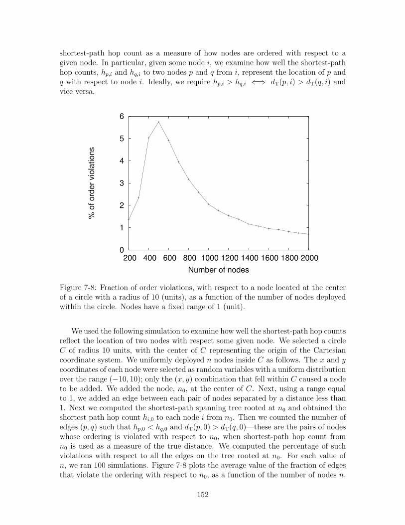
7-8 Fraction of order violations, with respect to a node located at the centerof a circle with a radius of 10 (units), as a function of the number ofnodes deployed within the circle. Nodes have a fixed range of 1 (unit). 152
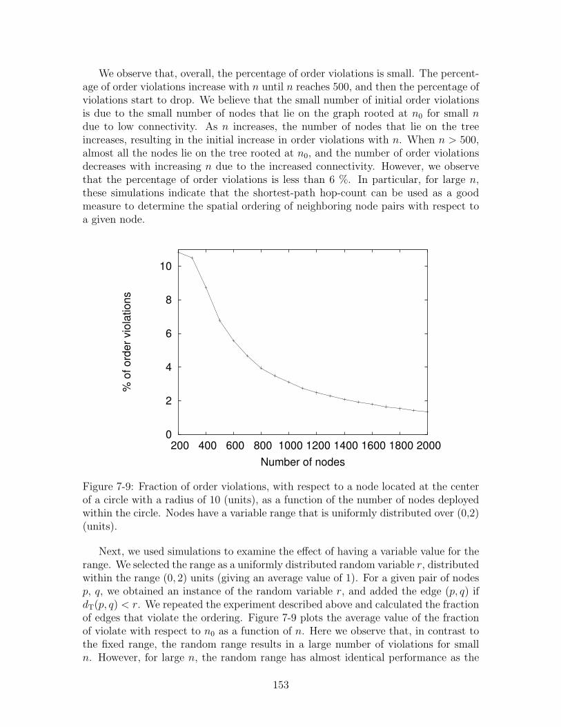
7-9 Fraction of order violations, with respect to a node located at the centerof a circle with a radius of 10 (units), as a function of the number ofnodes deployed within the circle. Nodes have a variable range that isuniformly distributed over (0,2) (units). . . . . . . . . . . . . . . . . . 153
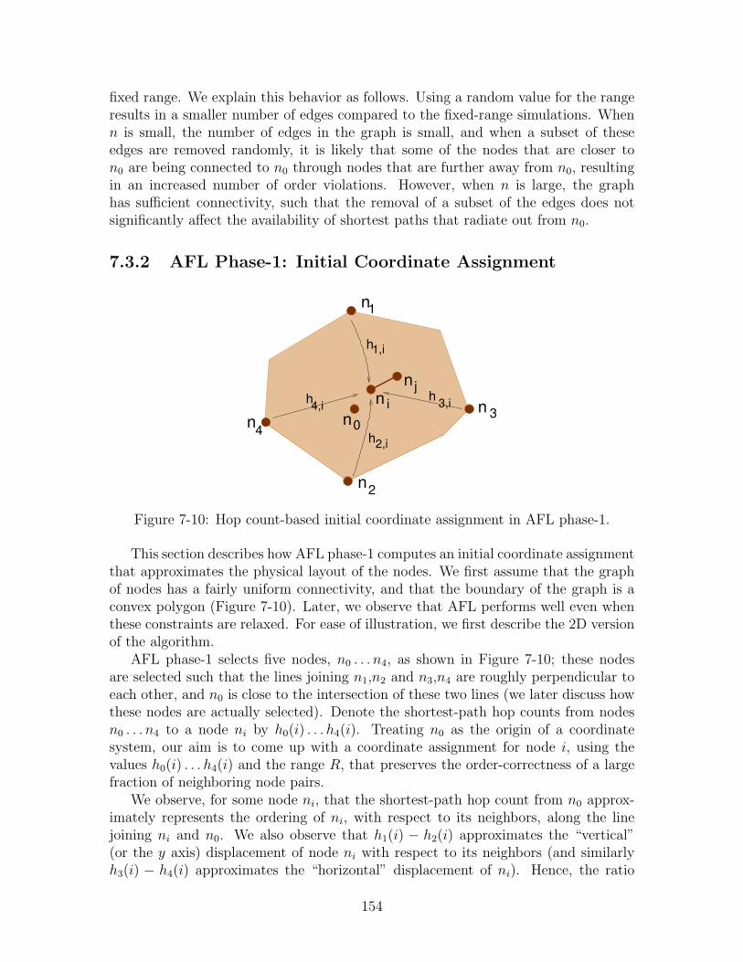
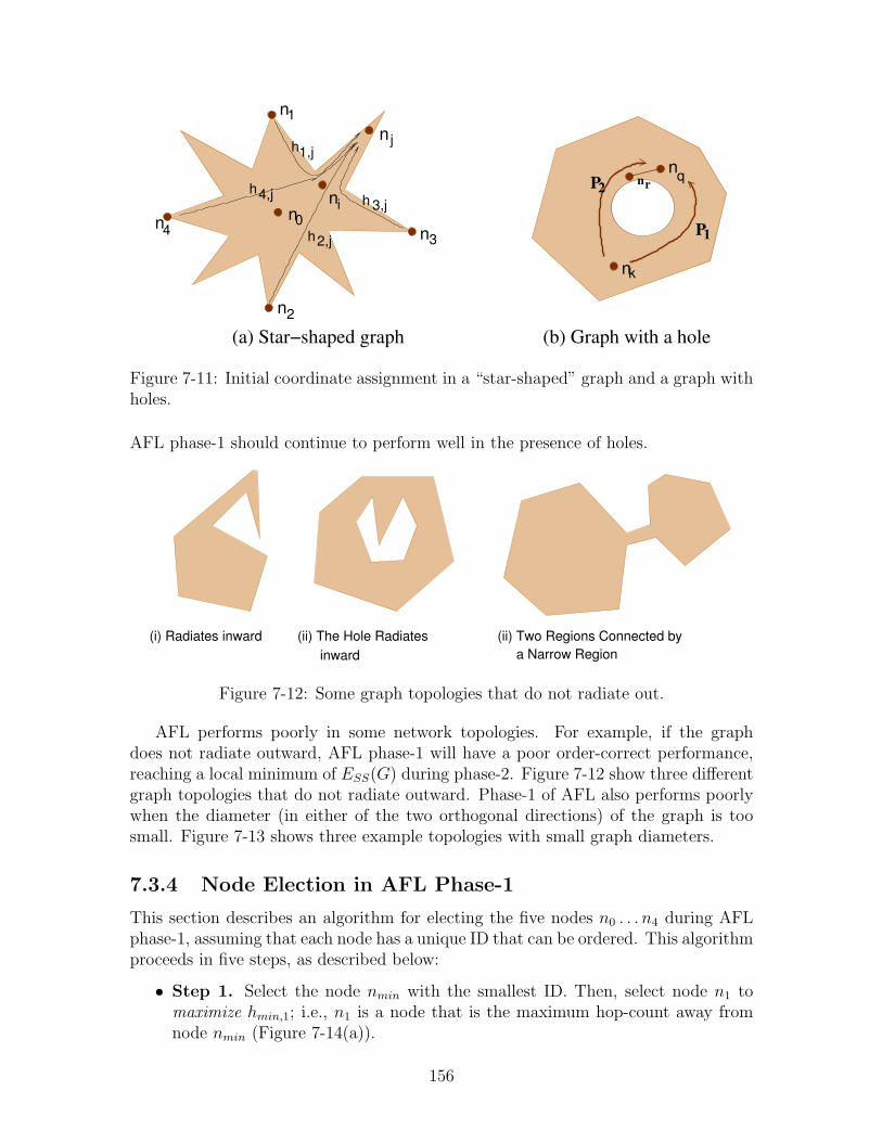
7-10 Hop count-based initial coordinate assignment in AFL phase-1. . . . . 154
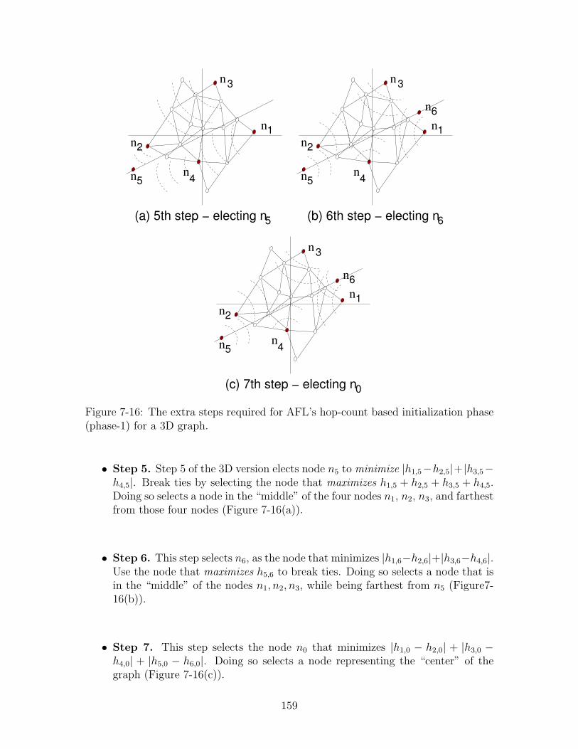
7-16 The extra steps required for AFL’s hop-count based initialization phase(phase-1) for a 3D graph. . . . . . . . . . . . . . . . . . . . . . . . . . 159
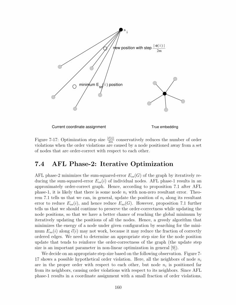
7-17 Optimization step size |~e(i)|2m
conservatively reduces the number of orderviolations when the order violations are caused by a node positionedaway from a set of nodes that are order-correct with respect to eachother. . . . . . . . . . . . . . . . . . . . . . . . . . . . . . . . . . . . 160
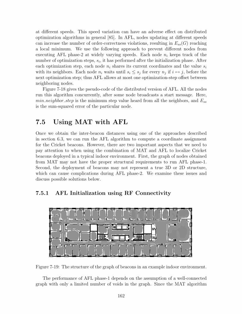
7-19 The structure of the graph of beacons in an example indoor environment.162
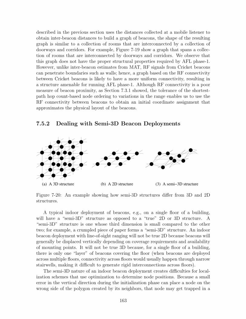
7-20 An example showing how semi-3D structures differ from 3D and 2Dstructures. . . . . . . . . . . . . . . . . . . . . . . . . . . . . . . . . . 163
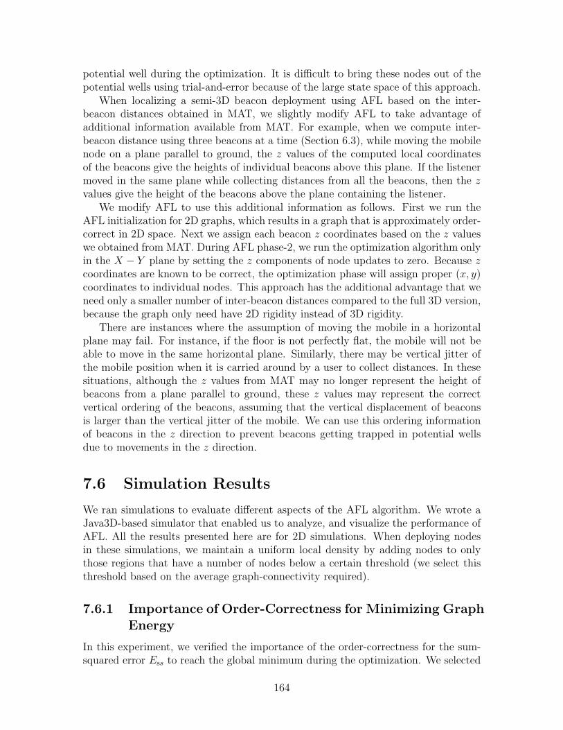
7-21 The fraction of ρ violations after AFL phase-1 vs. connectivity. . . . 165
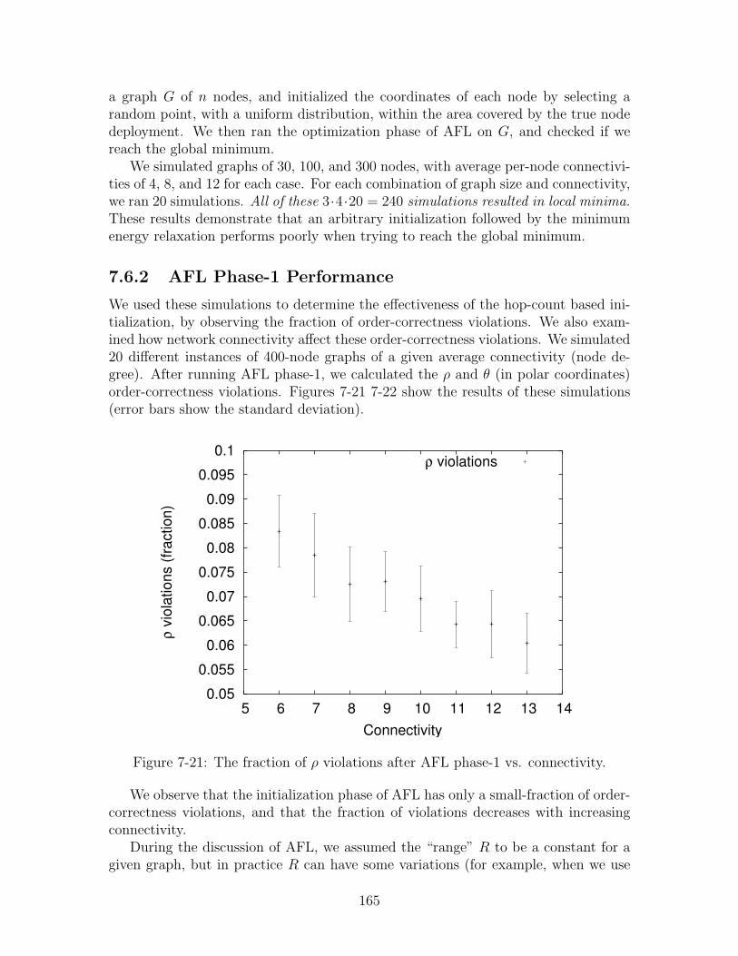
7-22 The fraction of θ violations after AFL phase-1 vs. connectivity. . . . . 166
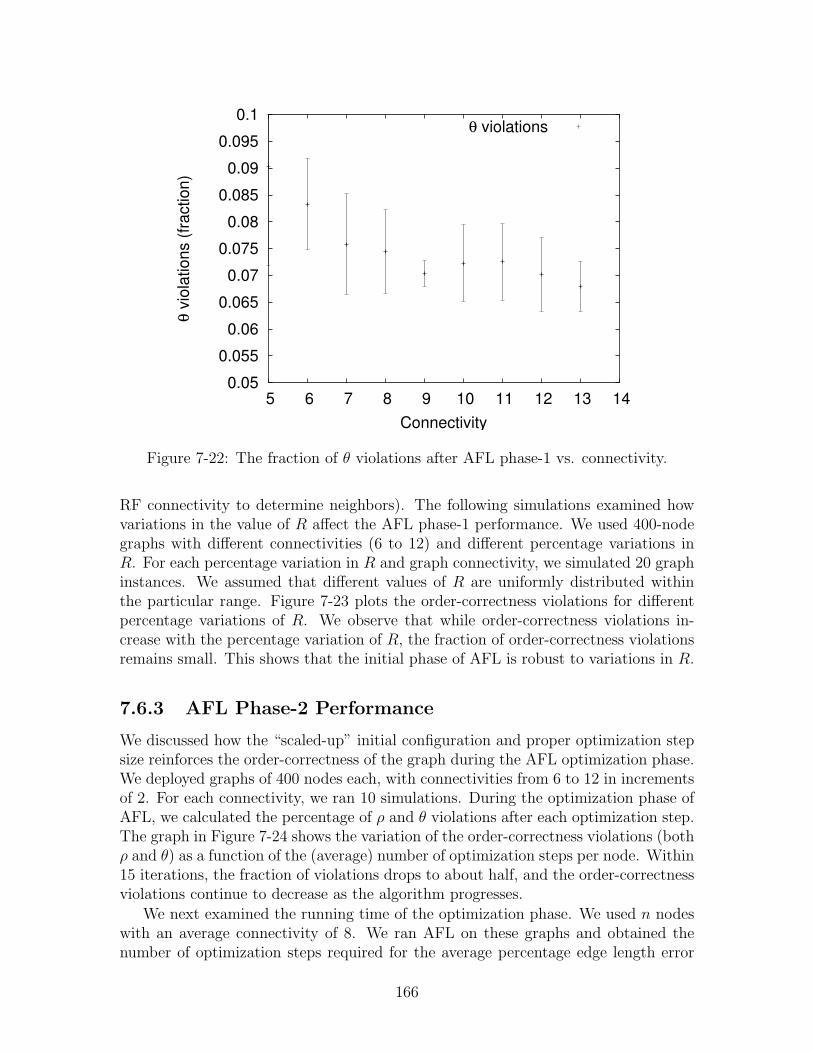
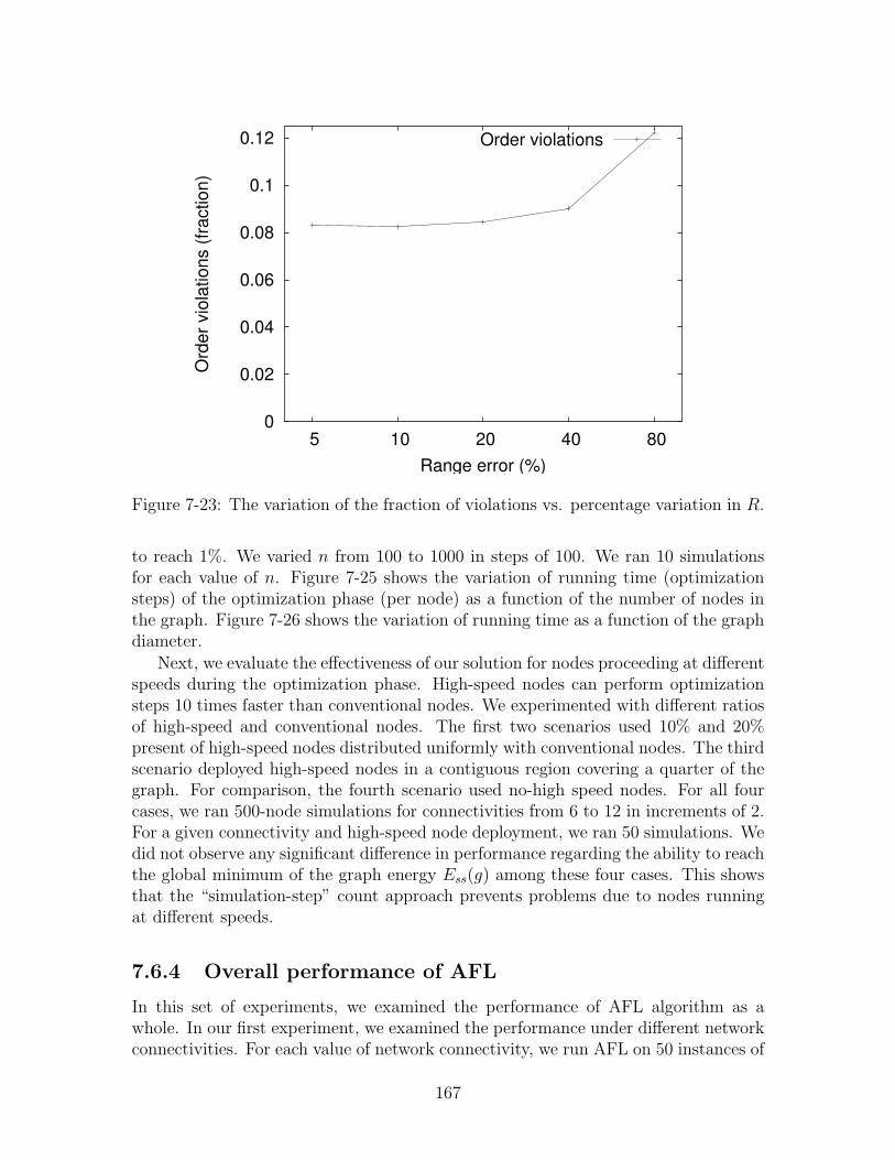
7-23 The variation of the fraction of violations vs. percentage variation in R.167
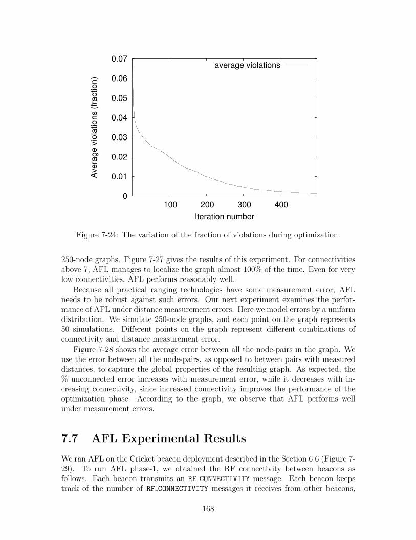
7-24 The variation of the fraction of violations during optimization. . . . . 168
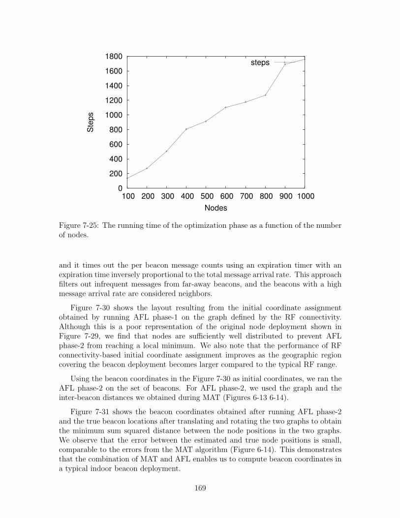
7-25 The running time of the optimization phase as a function of the numberof nodes. . . . . . . . . . . . . . . . . . . . . . . . . . . . . . . . . . . 169
19
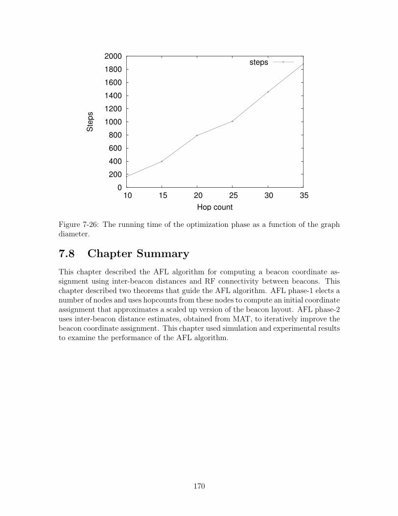
7-26 The running time of the optimization phase as a function of the graphdiameter. . . . . . . . . . . . . . . . . . . . . . . . . . . . . . . . . . 170
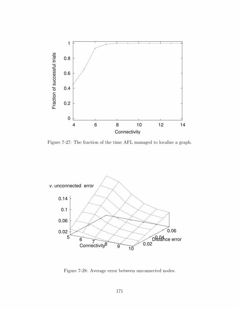
7-27 The fraction of the time AFL managed to localize a graph. . . . . . . 1717-28 Average error between unconnected nodes. . . . . . . . . . . . . . . . 1717-29 An indoor deployment of 24 nodes to evaluate the performance of MAT
and AFL (reproduced). . . . . . . . . . . . . . . . . . . . . . . . . . . 1727-30 Graph obtained after running the AFL initialization. . . . . . . . . . 1727-31 Coordinates obtained after running the AFL optimization, in compari-
son with the original node positions. The left-to-right distance betweenthe furthest nodes is about 10 meters. . . . . . . . . . . . . . . . . . . 173
Since time immemorial, knowing one’s location has been invaluable to humans foroutdoor navigation over land, sea, and air. Early navigators used equipment such asthe astrolabe, the sextant, and the octant to determine their location with respectto various celestial bodies [10]. In the twentieth century, advances in electronics andtelecommunication enabled technologies such as Long Range Navigation (LORAN),Radio Detection And Ranging (RADAR), and Global Positioning System (GPS) foroutdoor use [78, 36]. Outdoor location information has enabled applications as di-verse as tracking vehicles, logistical planning, locating people, resource discovery, andgames [59, 51, 30, 106, 35].
While outdoor location-aware applications are widespread today, our work is mo-tivated by the promise of indoor applications that can benefit from knowledge oflocation. Such applications span a wide range, including:
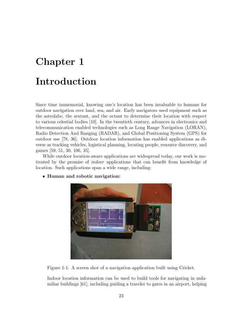
• Human and robotic navigation:
Figure 1-1: A screen shot of a navigation application built using Cricket.
Indoor location information can be used to build tools for navigating in unfa-miliar buildings [61], including guiding a traveler to gates in an airport, helping
23
users navigate (underground) train stations, helping visitors in a museum, di-recting visitors in an office building, etc. Figure 1-1 shows a screen shot of anindoor navigation application.
In robotic navigation, indoor location information can ease the complexity ofrobotic path planning. One interesting application enabled by indoor location isrobot-assisted elderly care, where a robot uses its own location and the locationof people to stay close to the person it is caring for [62].
• People and object tracking: Indoor location is also useful for applicationsthat track the location of people inside building. One example is an applicationthat tracks the location of different medical personnel inside a hospital to effi-ciently assign qualified personnel to various tasks. Other example applicationsinclude tracking and reporting the location of people in a user’s buddy list, andtracking the location of children in museums or schools [96].
Object and asset tracking is another category of indoor location-aware applica-tions. Examples include tracking books inside a library, tracking objects insidea warehouse, and tracking assets in an organization. The location of variousphysical resources such as printers, projects, and copiers also enable resourcediscovery applications that display the location of various resources in the vicin-ity of a user [3].
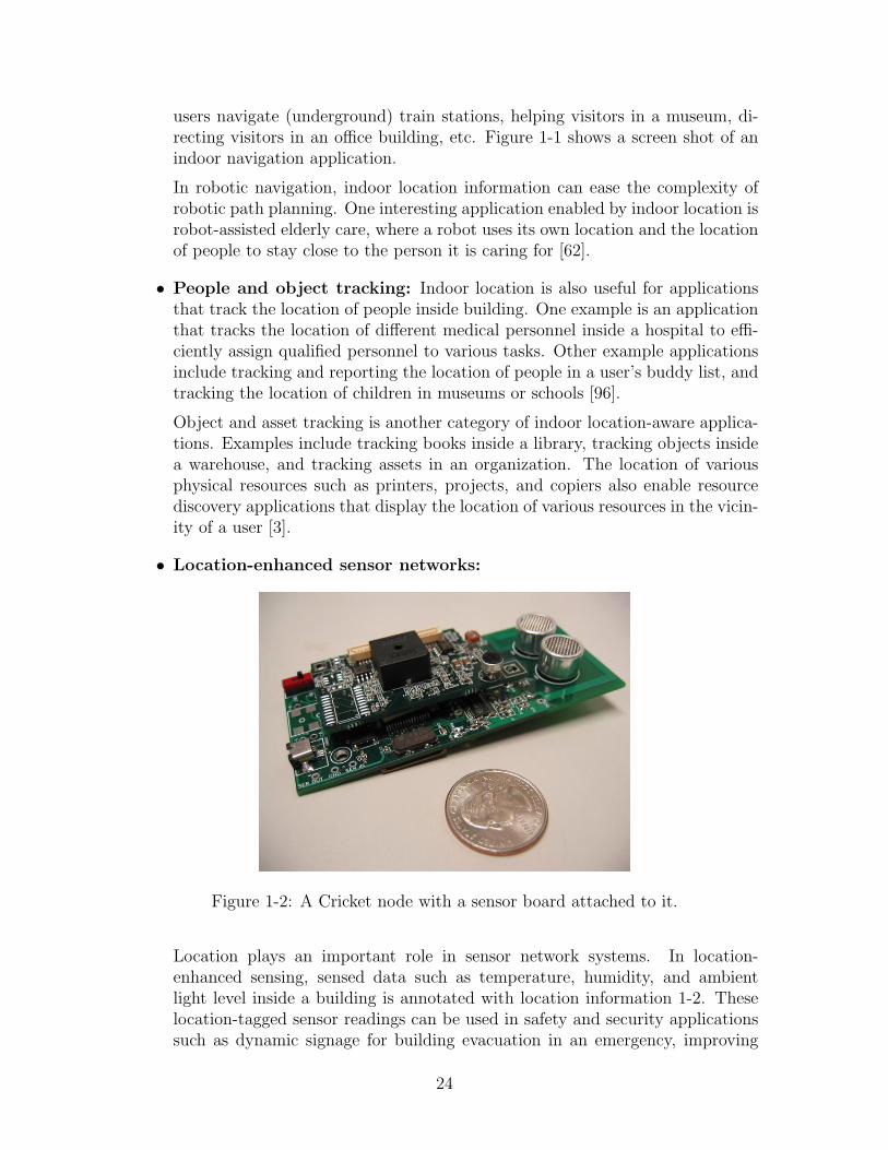
• Location-enhanced sensor networks:
Figure 1-2: A Cricket node with a sensor board attached to it.
Location plays an important role in sensor network systems. In location-enhanced sensing, sensed data such as temperature, humidity, and ambientlight level inside a building is annotated with location information 1-2. Theselocation-tagged sensor readings can be used in safety and security applicationssuch as dynamic signage for building evacuation in an emergency, improving
24
energy efficiency by turning on and off building services such as lighting andtemperature based on building occupancy, and efficient building maintenanceby quickly locating faulty building services [80, 60]. Location-enhanced sens-ing can also be used for monitoring conditions in difficult-to-access places ofbuildings—for example, monitoring air-conditioning ducts for mold growth andmonitoring the presence of pests [103].
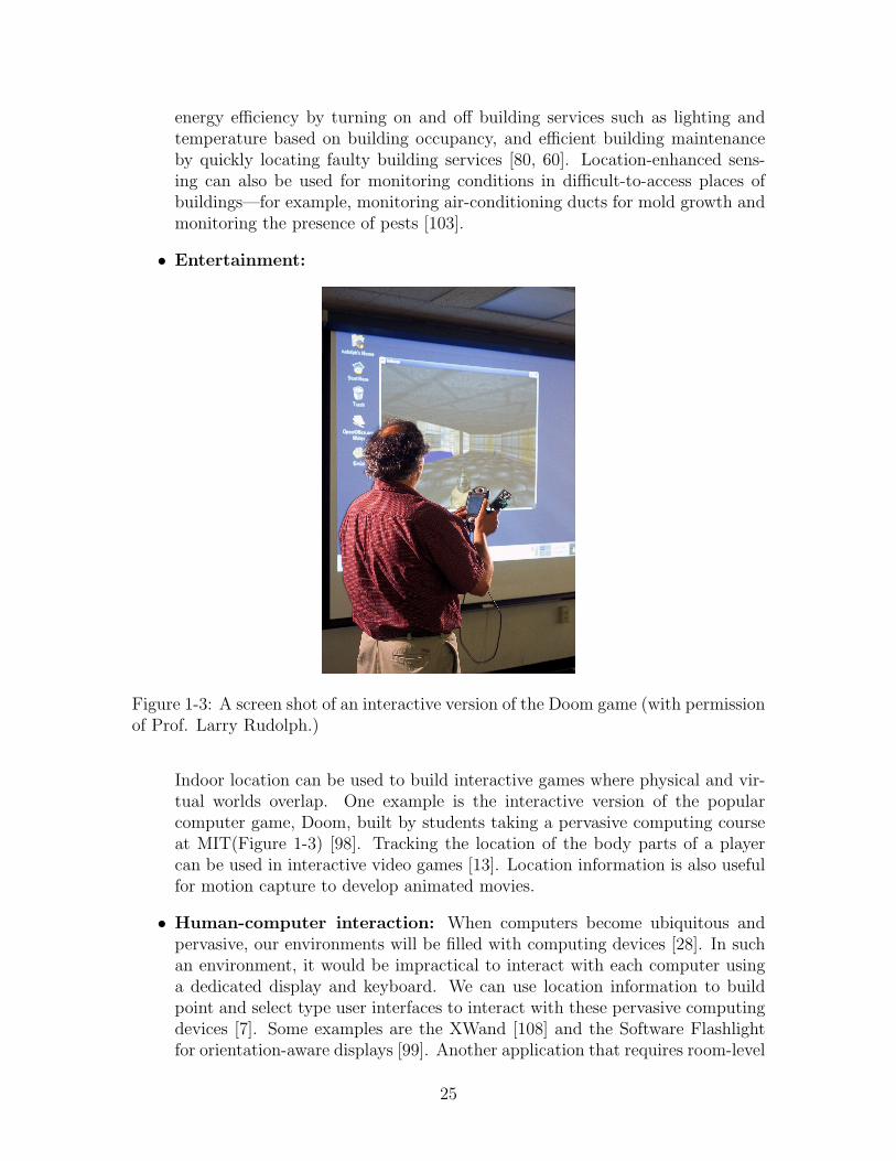
• Entertainment:
Figure 1-3: A screen shot of an interactive version of the Doom game (with permissionof Prof. Larry Rudolph.)
Indoor location can be used to build interactive games where physical and vir-tual worlds overlap. One example is the interactive version of the popularcomputer game, Doom, built by students taking a pervasive computing courseat MIT(Figure 1-3) [98]. Tracking the location of the body parts of a playercan be used in interactive video games [13]. Location information is also usefulfor motion capture to develop animated movies.
• Human-computer interaction: When computers become ubiquitous andpervasive, our environments will be filled with computing devices [28]. In suchan environment, it would be impractical to interact with each computer usinga dedicated display and keyboard. We can use location information to buildpoint and select type user interfaces to interact with these pervasive computingdevices [7]. Some examples are the XWand [108] and the Software Flashlightfor orientation-aware displays [99]. Another application that requires room-level
25
location is a video or an audio playback that follows the current location of theuser [68].
• Advertising: The location of a customer within a shopping mall can be usedfor sending targeted advertisements, possibly in combination with a map fornavigating the mall [1]. Location information can also be used for providingproduct information inside retail stores [97].
When we examine these applications, we observe that indoor location-aware appli-cations need a higher degree of accuracy, than typical outdoor applications. Mostoutdoor location systems that exist today are based on RF signals. An indoor envi-ronment presents harsh conditions for RF propagation because of the reflections andattenuation caused by various metallic objects. Because of this, traditional outdoorlocation systems have poor indoor performance.
From the above list of example indoor location-aware applications, we observethat different types of applications need different types of location information. Weidentify following three types of location information:
• Space: Space is defined as a region within some boundary. Examples are roomsand portions of rooms. A room is defined by the walls surrounding it, while asection of a room is defined by a collection of walls and virtual boundaries thatare used to demarcate different sections of a room. Space is the most naturalform of location information for humans; for example, we often use terms suchas “my office” and “living room” refer to different spaces. A space is bestdenoted by some human-readable text string.
• Position. Position is defined as a point in some coordinate system. For in-stance, the GPS system uses a global spherical coordinate system (latitude,longitude, and altitude) to uniquely identify a position relative to the earth.Building plans, deeds, and city maps all use two-dimensional (2D) coordinatesystems to identify the location and the size of different objects. If the positionis only used to identify the size of objects and determine how different objectsare located with respect to each other, then a local coordinate system with anarbitrary origin can be used. A 2D or 3D local coordinate system can be trans-lated to a global coordinate system if the global and local coordinates of threeor four different points are known. We note that the position of some objector a person is not clearly defined because they occupy a region of space ratherthan a single point. Unless otherwise stated, we define the position of a useror an object as the position of the location sensor carried by the person or theobject.
• Orientation: Orientation is usually denoted by the angle between a given di-rection and the true north. True north is defined by the meridians of longitude.True north is different from the magnetic north, which is the direction a mag-netic compass needle points toward. It is also possible to define orientation asthe offset between the direction of interest and the coordinate axes, within some
26
coordinate system. If the coordinate system is a local coordinate system, suchas a coordinate system defined within a building, then the orientation informa-tion also becomes local. Some indoor applications, such as an application thatneeds to identify the object a person is pointing at, may be able to use eitherlocal or global orientation (the orientation with respect to true north), whilesome other applications, such as an application that displays a map adjustedto the direction a handheld device is pointing, may need global orientation in-formation. An application for locating objects inside a ship or an aircraft mayneed only local orientation information. If only local orientation information isknown, we can translate it to global orientation if the angle of rotation betweenthe local and the global orientation is known.
This dissertation describes a location system that provides accurate indoor loca-tion information in the forms of space, position, and orientation.
1.1 The Cricket System
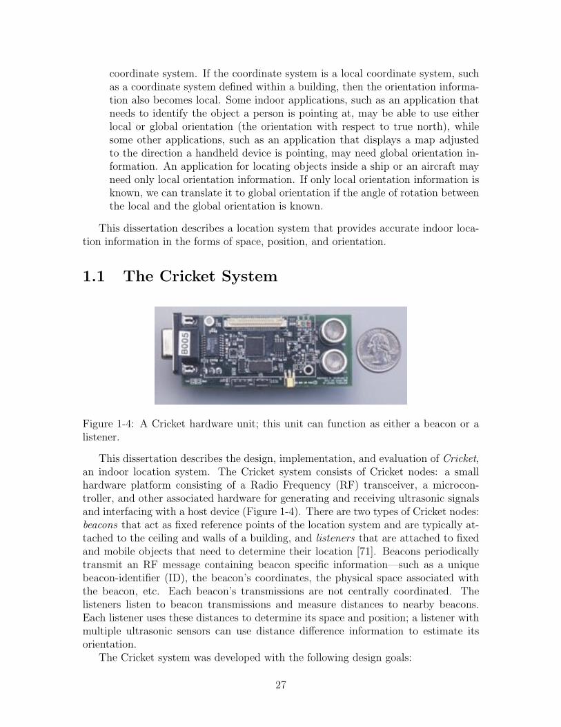
Figure 1-4: A Cricket hardware unit; this unit can function as either a beacon or alistener.
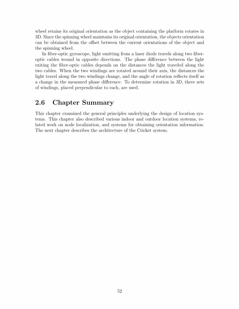
This dissertation describes the design, implementation, and evaluation of Cricket,an indoor location system. The Cricket system consists of Cricket nodes: a smallhardware platform consisting of a Radio Frequency (RF) transceiver, a microcon-troller, and other associated hardware for generating and receiving ultrasonic signalsand interfacing with a host device (Figure 1-4). There are two types of Cricket nodes:beacons that act as fixed reference points of the location system and are typically at-tached to the ceiling and walls of a building, and listeners that are attached to fixedand mobile objects that need to determine their location [71]. Beacons periodicallytransmit an RF message containing beacon specific information—such as a uniquebeacon-identifier (ID), the beacon’s coordinates, the physical space associated withthe beacon, etc. Each beacon’s transmissions are not centrally coordinated. Thelisteners listen to beacon transmissions and measure distances to nearby beacons.Each listener uses these distances to determine its space and position; a listener withmultiple ultrasonic sensors can use distance difference information to estimate itsorientation.
The Cricket system was developed with the following design goals:
27
• Small form factor. We wanted to build a system that can be easily used withmobile devices and sensors. This goal required the hardware implementation tobe smaller than the typical handheld device.
• Accuracy. Since indoor environments contain closely spaced objects that wemay want to uniquely identify by their locations, we wanted a location systemthat provides a position accurate to a few centimeters.
• Scalability. We anticipate that a large number of users and objects will requirelocation information. Hence, we wanted a system that scales with the numberand density of users.
• User privacy. The user-tracking nature of some previous location systemscaused privacy concerns. Our aim was to build a location system that enablesa variety of privacy policies, depending on end-user applications.
• Ease of deployment and configuration. We wanted to build a locationsystem that is easy to deploy and configure.
1.2 Challenges
Cricket listeners use measured distances to nearby beacons to determine listener lo-cation. Since we need accurate location information, the listeners need to be ableto measure these distances accurately. This dissertation describes how beacons usea combination of RF and ultrasonic signal transmissions to enable accurate distancemeasurements at the listener. However, the uncoordinated beacon transmissions caninterfere, resulting in incorrect distance samples. This dissertation describes a combi-nation of beacon scheduling algorithms and listener filtering algorithms that preventincorrect distance samples while maintaining the distributed system architecture.
For a listener to compute its position using measured distances to nearby beacons,the listener needs to know the coordinates of these beacons. To achieve ease of deploy-ment and configuration of the system, we developed algorithms that enable beaconsto configure themselves with a coordinate assignment that reflects their true physicallayout. These algorithms eliminate the the need for manual coordinate configuration.
The first algorithm produces a set of inter-beacon distances that represents therelative positions of the beacons. However, for a variety of reasons including the line-of-sight requirements of ultrasound-based ranging, it is impossible for the beacons tomeasure these inter-beacon distances directly.
After inter-beacon distances are obtained, it is necessary to compute a beaconcoordinate assignment that satisfies these distances. Since the beacons are deployedindoors, it is impractical to assume the availability of other location technologies,such as GPS, for aiding the beacon coordinate assignment. Hence, Cricket requiresa beacon coordinate assignment algorithm that can compute coordinates using onlythe inter-beacon distances; for obtaining accurate beacon coordinates, this algorithmmust tolerate distance measurement errors well.
28
1.3 Contributions of this Dissertation
This dissertation makes the following contributions. It describes the design, imple-mentation, and evaluation of the hardware, software, and algorithmic components ofthe Cricket system. The Cricket hardware platform consists of the following majorcomponents: an RF transceiver for sending an receiving RF messages, a microcon-troller that runs various algorithms and circuitry for transmitting and receiving ultra-sonic signals. The software running on Cricket nodes, apart from handling RF andultrasonic transmissions, also provides an API to set and retrieve different systemparameters.
Indoor location systems built prior to Cricket had centralized architectures, wherea collection of sensors or transmitters spread across a building were wired to a centralcontroller (see Chapter 2). Cricket was the first indoor location system that used anall-wireless, distributed infrastructure.
Cricket also introduced the importance of location in the form of space for devel-oping location-aware applications. This dissertation describes a beacon deploymentstrategy that detects boundaries between spaces accurately for determining listenerspace.
Cricket uses a “passive mobile” approach, where the mobile node passively listensto transmissions from the deployed infrastructure and computes the mobile’s positionlocally. This passive mobile architecture scales well with the number of mobile devices.This architecture also enables applications that preserve user privacy.
Cricket provides all three forms of location information—space, position, and ori-entation—within a local coordinate system. To our knowledge, Cricket is the onlylocation system that provides all these three types of location information in a smallform-factor, within a local frame of reference.
We have developed, implemented, and evaluated the following algorithms in Cricket:
• Beacon scheduling. The distributed Cricket architecture consisting of autonomousbeacons with periodic transmissions requires energy-efficient transmission algo-rithms that avoid interactions between multiple beacon transmissions. We havedeveloped and evaluated a beacon scheduling algorithm that aims to minimizeinteractions between beacon transmissions.
• Interaction detection. We developed a interaction detection algorithm to detectbeacon transmission interactions that may otherwise lead to erroneous distanceestimates.
• Outlier rejection. Although the scheduling and interaction detection algorithmscan prevent and detect all the inter-beacon interactions under ideal RF prop-agation models, real-world imperfections such as RF dead-spots cause somebeacon interactions resulting in outlier measurement samples at listeners. Wehave developed two algorithms for filtering out these outliers.
The MinMode algorithm [71], which collects multiple distance samples and se-lects the measurement with the maximum occurrence, is suitable for static or
29
slowly moving listeners. For continuously moving listeners, we use a Kalmanfilter-based approach to detect outliers [92]. In this approach, the listener usesa simplified model to predict its position when it receives a new distance sam-ple, and uses this position estimate to compute an estimated distance to thecorresponding beacon. The listener uses the difference between the measuredand the estimated distances to reject or accept the new sample.
• Phase difference estimation for orientation. Cricket listeners determine orien-tation using differential distance estimates. This dissertation presents a uniquesensor placement and signal analysis technique that resolves the phase ambigu-ity problem in phase-difference based differential distance estimation [72].
• Anchor-free localization. Once deployed, Cricket beacons need to be configuredwith a coordinate assignment that satisfies the physical layout of the beacons.We have developed AFL, an anchor-free distributed localization algorithm, thatenables beacons to configure themselves with a valid coordinate assignment [70].The AFL algorithm runs in two phases. First, it uses RF connectivity to com-pute an initial coordinate assignment resulting in a beacon a topology thatresembles a scaled and unfolded version of the true configuration. In the secondphase, it uses inter-beacon distances to run an iterative optimization procedureto minimize the error between the current beacon configuration and the trueembedding.
• Mobile-assisted topology generation. The beacon localization algorithm usesinter-beacon distances to compute beacon coordinates. However, obstacles andthe characteristics of the ultrasonic sensors used in Cricket prevent beacons frommeasuring inter-beacon distances directly. The localization algorithm needs asufficient number of inter-beacon distances such that a coordinate assignmentthat satisfies these distances correctly reflects the true beacon deployment. Wehave developed MAT, a mobile-assisted topology generation algorithm to com-pute a sufficient number of inter-beacon distances using distance measurementsat a mobile listener [73].
It must be noted that, although these algorithms were developed and evaluatedfor the RF and ultrasound-based distance measurement apparatus in Cricket, all thealgorithms, except for the beacon scheduling and interaction avoidance, can be usedwith any ranging technology.
We provide simulation and measurement results on the performance of the in-dividual algorithms and the complete Cricket system. Cricket achieves a distancemeasurement accuracy of 4-5 cm within a 80o cone from a given beacon. Cricketachieves a boundary detection accuracy of about 1 cm, a position accuracy of 10-12cm, and an orientation accuracy of 3o − 5o. The current implementation of Crickethas a form factor which is amenable to be used with handheld devices [24]. Crickethardware implementation is commercially available from Crossbow technologies [26].
30
1.4 Organization of the Dissertation
The remainder of this dissertation presents the implementation and evaluation of theCricket indoor location system. Chapter 2 presents general background and relatedwork on location systems. We present the hardware and software architecture ofCricket in Chapter 3. Chapter 4 describes the RF and ultrasound-based distancemeasurement in Cricket; this chapter describes algorithms for beacon interactionavoidance, and evaluates the Cricket system scalability performance. Chapter 5 de-scribes the algorithms for obtaining different types of listener location informationusing distance measurements to beacons. In Chapter 6, we present the MAT algo-rithm, which computes inter-beacon distances and build a rigid structure for beaconlocalization, using distance samples at a mobile listener. Chapter 7 describes theAFL algorithm which computes a beacon coordinate assignment using inter-beacondistances obtained from MAT. Finally, Chapter 8 summarizes our work and describepossible future directions for improving Cricket performance.
31
32
Chapter 2
Related Work
A location system provides the current location of an object within a given coordinatesystem. There are two basic approaches to determining the location of an object.
• Location from landmarks. In this approach, the location system is imple-mented by selecting a set of landmarks or reference points with known coordi-nates. The reference points can be either fixed or moving within the selectedcoordinate system (e.g. GPS [36]). If the reference points are moving, theyshould follow a predefined trajectory so that their coordinates can be deter-mined at a given instance. For example, consider three reference points A, B,and C located in a 2D coordinate system. Let d1, d2, and d3 be the measureddistances to some object O from these points. If we know the coordinates ofthe three reference points at the time each measurement was taken, then wecan compute the coordinates of O uniquely by solving a system of equations.
A slightly different form of landmark-based location systems uses boundaries aslandmarks. In these systems, boundaries are used to demarcate different physi-cal spaces. The boundaries themselves are defined by line segments and curvesin some coordinate system. Some examples are: walls that define individualrooms of a building, state-boundaries that identify different states on a map,etc.
• Location from dead-reckoning. Dead-reckoning determines the position ofan object with respect to some starting point using the dynamics of motion ofthat object. For instance, if an object O starts moving from some point P alonga direction θ at a constant velocity v, its position coordinates at time t are givenby (vt cos θ, vt sin θ). Dead-reckoning relies on the ability of the moving objectto accurately measure its dynamics. Since position estimation requires themeasured dynamics such as velocity and acceleration to be integrated in time,dead-reckoning suffers from an accumulation of measurement errors. Becauseof this shortcoming, most location systems are implemented using landmarks,or using a combination of landmarks and dead-reckoning. In the rest of thischapter, we limit our discussion of location systems to landmark-based systems.
33
This chapter surveys various location systems and the techniques they use to inferlocation. Section 2.1 gives a general overview of different techniques that can be usedto build location systems. Section 2.2 examines different outdoor location systemsthat exist today. Section 2.3 describes several indoor location systems. Section 2.4gives an overview of the node localization problem and also describes related work innode localization. Section 2.5 examines different techniques for obtaining orientationinformation.
2.1 Overview of Techniques to Determine Loca-
tion
Landmark-based systems need a way by which an object can determine its positionbased on its proximity to the reference points. The following different approachesmay be used to determine the position of an object within a landmark-based system.
• Distance and angle. This is the most widely used technique for position esti-mation. Usually, these distance and angle measurements to the reference pointsare used to compute the position of the object by triangulation. Outdoor loca-tion systems such as GPS [36], RADAR [78], and LORAN [] use this approachto determine location (see Section 2.2).
• Signal signature. In this approach, the reference points transmit some signal,usually over RF. The position of an object is determined by measuring thestrength of the signals received from one or more reference points. The measuredsignal strength is used as a signature to uniquely identify a given point in spacewith respect to the landmarks. It is also possible to use an approach wherethe object transmits and the received signal strength at multiple fixed referencepoints serve as the signature. Several indoor location systems use this techniqueto determine a mobile node’s position based on the RF signal strength of accesspoints [6, 15, 56, 41, 79, 109].
• Visibility. In this approach, an object is associated with a given referencepoint if that object can receive some signal transmitted by the reference pointor visa versa. These systems are usually engineered such that at any givenlocation an object can receive only one reference point’s transmission. TheActive Badge [105] location system and the CoolTown [55] project use thisapproach.
2.1.1 Distance Measurement Techniques
Distance measurement is a widely used approach for location estimation. Thereare three common techniques for measuring the distance to an object from a givenreference point:
34
• Time-of-flight. This technique measures the time t taken for some signal totraverse the path between two points (the reference point and the object). Ifthe speed of the signal is v, the distance d is given by d = v × t. For example,GPS uses the time of flight of RF signals to estimate the distance between GPSsatellites and the GPS receiver [36].
• Time-Difference-of-Arrival (TDOA). TDOA-based schemes measure thedistance between given two points using two signals with different speeds thattraverse the same path between the two points. Consider two signals A and Bwith speeds vA and vB sent simultaneously by a transmitter. If vA > vB, thensignal B lags behind signal A as they propagate. Let t denote this time lag ata receiver located at a distance d from the transmitter. Then,
d =t
1vA− 1
vB
.
For example, Cricket uses TDOA of RF and ultrasonic signals to measure dis-tance to the reference points.
• Image processing. This technique is widely used in passive auto-focus cam-eras. Here a microprocessor moves a motor-driven lens located in front of aCharge Coupled Device (CCD) sensor array until a focused image of a target isformed on the sensor. Once the image is in focus, for a given lens, the distancebetween the CCD sensor and the lens l defines the distance d to the target; thedistance d can be computed from l and the F number of the lens using the lawsof geometric optics [45].
2.2 Outdoor Location Systems
Traditionally, location systems were built to support outdoor navigation applicationssuch as navigating military and commercial ships and aircrafts. Most traditionallocation systems were designed for outdoor applications.
Location information was an invaluable resource for early navigators. These nav-igators used the Earth as their frame of reference, determining their location bymeasuring the angle of different celestial bodies relative to the horizon using toolssuch as the quadrant and the sextant [10]. Celestial bodies act as a collection ofnatural reference points moving in a predictable path relative to the earth.
The twentieth century saw radical improvements in the quality and accuracy ofoutdoor location systems. We briefly survey six important systems here: SONAR,VOR, LORAN, RADAR, GPS, and E-911.
2.2.1 Sound Navigation and Ranging (SONAR)
SONAR was developed during the First World War for underwater navigation of sub-marines. SONAR uses an ultrasonic transmitter to emit ultrasonic pulses, which get
35
reflected by obstacles such as ships in the sea. The time of flight of these reflectedsignals is used to compute the distance to the obstacle. Some sonar systems emit anultrasonic beam that can be rotated either mechanically or using an array of trans-mitters fed with phase-shifted signals. For a rotated beam, the angle of rotation ofthe beam determines the angle of the obstacle with respect to the object transmittingthe ultrasonic signal. Thus SONAR estimates the position of objects with respect tothe coordinate frame defined by the transmitter.
2.2.2 Very High Frequency Omni-directional Range (VOR)System
N
θ
N
α
VOR ground station
Heading of the aircraft
β
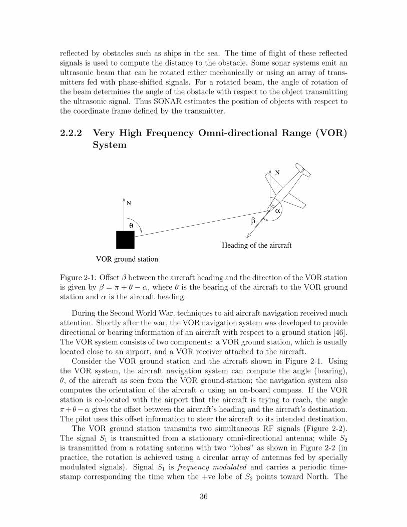
Figure 2-1: Offset β between the aircraft heading and the direction of the VOR stationis given by β = π + θ − α, where θ is the bearing of the aircraft to the VOR groundstation and α is the aircraft heading.
During the Second World War, techniques to aid aircraft navigation received muchattention. Shortly after the war, the VOR navigation system was developed to providedirectional or bearing information of an aircraft with respect to a ground station [46].The VOR system consists of two components: a VOR ground station, which is usuallylocated close to an airport, and a VOR receiver attached to the aircraft.
Consider the VOR ground station and the aircraft shown in Figure 2-1. Usingthe VOR system, the aircraft navigation system can compute the angle (bearing),θ, of the aircraft as seen from the VOR ground-station; the navigation system alsocomputes the orientation of the aircraft α using an on-board compass. If the VORstation is co-located with the airport that the aircraft is trying to reach, the angleπ+θ−α gives the offset between the aircraft’s heading and the aircraft’s destination.The pilot uses this offset information to steer the aircraft to its intended destination.
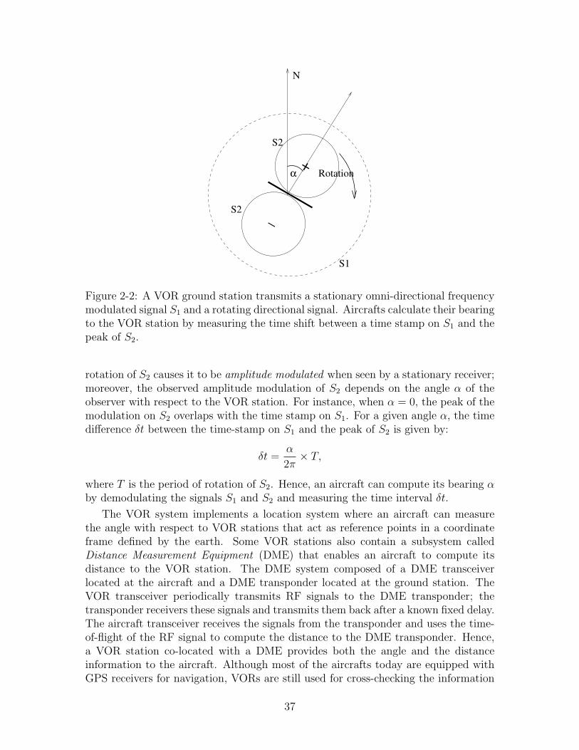
The VOR ground station transmits two simultaneous RF signals (Figure 2-2).The signal S1 is transmitted from a stationary omni-directional antenna; while S2
is transmitted from a rotating antenna with two “lobes” as shown in Figure 2-2 (inpractice, the rotation is achieved using a circular array of antennas fed by speciallymodulated signals). Signal S1 is frequency modulated and carries a periodic time-stamp corresponding the time when the +ve lobe of S2 points toward North. The
36
+
_
S1
Rotation
S2
S2
N
α
Figure 2-2: A VOR ground station transmits a stationary omni-directional frequencymodulated signal S1 and a rotating directional signal. Aircrafts calculate their bearingto the VOR station by measuring the time shift between a time stamp on S1 and thepeak of S2.
rotation of S2 causes it to be amplitude modulated when seen by a stationary receiver;moreover, the observed amplitude modulation of S2 depends on the angle α of theobserver with respect to the VOR station. For instance, when α = 0, the peak of themodulation on S2 overlaps with the time stamp on S1. For a given angle α, the timedifference δt between the time-stamp on S1 and the peak of S2 is given by:
δt =α
2π× T,
where T is the period of rotation of S2. Hence, an aircraft can compute its bearing αby demodulating the signals S1 and S2 and measuring the time interval δt.
The VOR system implements a location system where an aircraft can measurethe angle with respect to VOR stations that act as reference points in a coordinateframe defined by the earth. Some VOR stations also contain a subsystem calledDistance Measurement Equipment (DME) that enables an aircraft to compute itsdistance to the VOR station. The DME system composed of a DME transceiverlocated at the aircraft and a DME transponder located at the ground station. TheVOR transceiver periodically transmits RF signals to the DME transponder; thetransponder receivers these signals and transmits them back after a known fixed delay.The aircraft transceiver receives the signals from the transponder and uses the time-of-flight of the RF signal to compute the distance to the DME transponder. Hence,a VOR station co-located with a DME provides both the angle and the distanceinformation to the aircraft. Although most of the aircrafts today are equipped withGPS receivers for navigation, VORs are still used for cross-checking the information
37
from GPS.
2.2.3 Long Range Navigation (LORAN) System
The LORAN system provided guidance information for aircrafts and ships duringthe latter part of the Second World War. The LORAN system consists of a masterRF transmitter and several slave RF transmitters at fixed known locations. Themaster transmitter periodically transmits an RF signal; the slave transmitters, aftera fixed delay from receiving the master transmission, retransmit the same signal.The LORAN receivers, carried by ships and aircrafts, compute the time difference ofarrival of signals for each slave and the master.
M
S2
S1
p1
p2
d1 d
R
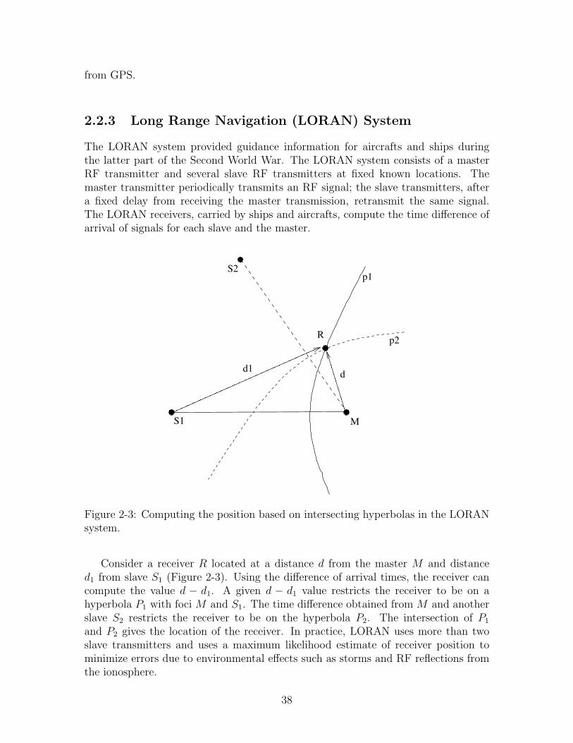
Figure 2-3: Computing the position based on intersecting hyperbolas in the LORANsystem.
Consider a receiver R located at a distance d from the master M and distanced1 from slave S1 (Figure 2-3). Using the difference of arrival times, the receiver cancompute the value d − d1. A given d − d1 value restricts the receiver to be on ahyperbola P1 with foci M and S1. The time difference obtained from M and anotherslave S2 restricts the receiver to be on the hyperbola P2. The intersection of P1
and P2 gives the location of the receiver. In practice, LORAN uses more than twoslave transmitters and uses a maximum likelihood estimate of receiver position tominimize errors due to environmental effects such as storms and RF reflections fromthe ionosphere.
38
2.2.4 Aircraft RADAR
RADAR systems are used in diverse applications such as aircraft navigation, detect-ing enemy aircrafts, detecting speeding vehicles, and predicting weather. The basicRADAR architecture consists of a radio transmitter and a receiver connected to arotating antenna. The radio transmitter transmits shorts bursts of radio signals,which reflect from objects such as aircrafts, and are received at the radio receiver.The measured time difference between the transmission of a pulse and its reception,∆T , and the distance D to the reflecting object can be obtained from the equationD = 0.5c∆T , where c is the speed of the RF signals.
The angle of rotation, θ, of the RADAR antenna, at the time of the reflection,gives the orientation of the object with respect to the earth. Hence the values (D, θ)gives the position of the object (in polar coordinates) with respect to the RADARantenna on a 2D plane.
2.2.5 Global Positioning System (GPS)
The GPS system consists of twenty seven satellites (as of May 2005) that orbit theearth [36, 48]. Because the satellites follow well-known orbits, their positions arepredictable. Each satellite transmits an RF signal encoded with a unique bit pattern.The data streams from different satellites are synchronized using atomic clocks. Whena GPS receiver receives signals from multiple satellites, the receiver measures the timeshift between the data streams from different satellites. Since the satellite positionsare known, the receiver can use the time shifts between signals from any four satellitesto solve for the four unknowns that represent the receiver’s position in 3D and thecurrent time (the time is treated as an unknown, because the clock of the receiver isnot as accurate as the clocks carried by satellites).
Using civilian GPS signals, it is possible to achieve a receiver position accuraciesof about fifteen to thirty meters. The main sources of error in receiver position esti-mation are the additional propagation delays that occur when the signals propagatethrough the ionosphere and the atmosphere, along the path from the satellites tothe receiver. Differential GPS (DGPS) reduces the position estimation error downto about five meters by using GPS signals received at a known position. The GPSreceiver at the known position estimates the additional delays caused by ionosphericand atmospheric effects on the signals received from individual satellites, and relaythis information to other nearby GPS receivers. These GPS receivers subtract outthese additional delays during position estimation [48].
In indoor environments, signals from GPS satellites get attenuated and reflectedby various metallic objects [31]. Unlike ionospheric and atmospheric effects thathappen at a distance far away from a GPS receiver, effects due to these metallicobjects vary rapidly from point to point inside a building. Because of this, it is notpossible to use techniques such as DGPS to overcome position estimation errors dueto these indoor effects. Thus, indoor GPS performance has fundamental limitationsthat result in much larger position estimation errors compared to outdoors.
39
2.2.6 Mobile Phone Location Systems for E-911
The United States Federal Communications Commission’s (FCC) E-911 directive [30]requires that a mobile phone operator must be able to provide the location of a userdialing 911.
Some cell phone operators provide this location information using mobile phonesequipped with GPS receivers, while other operators use information gathered from thecell phone network to locate callers. The network-based approach uses a combinationof RF time of flight and Angle of Arrival (AOA) of mobile phone’s signals at thecellular towers to compute the caller’s location. The AOA is obtained by comparingthe received RF signal strength at multiple antennas on the cellular tower.
2.3 Indoor Location Systems
Traditional location systems such as VOR/DME, LORAN, RADAR, GPS, etc. thatprovide location information for outdoor navigation are characterized by referencepoints deployed at known positions. The reference points, in the form of RF groundstations, satellites etc., constitute expensive infrastructure. Most of these systemsuse RF signals for providing location information, providing a typical accuracy ofseveral meters, which is sufficient for most outdoor applications. Indoor location-aware applications operate in harsher environments that impede RF propagationand these applications often require higher accuracy. On the other hand, indoorapplications require a smaller coverage area compared to a typical outdoor system,and it is often desirable to limit the coverage area to a single organization. As a result,several research groups have developed a number of location technologies specificallytailored for indoor applications.
2.3.1 In-building RADAR
The RADAR system developed at Microsoft Research implements a location serviceutilizing the information obtained from an already existing RF data network [6]. Ituses the RF signal strength as an indicator of the distance between a transmitter anda receiver. This distance information is then used to locate a user by triangulation.During an off-line phase; the system builds a data base of RF signal strength at aset of fixed receivers, for known transmitter positions. During the normal operation,the RF signal strength of a transmitter as measured by the set of fixed receivers, issent to a central computer, which examines the signal-strength database to obtainthe best fit for the current transmitter position.
Many other groups have also developed 802.11-based location systems in recentyears [15, 56, 41, 79, 109]. A study has found that such 802.11-based indoor locationsystems have fundamental limits that result in a median position estimation error of' 3 m [32].
40
2.3.2 The Active Bat Location System
In the Active Bat system, various objects within the system are tagged by attachingsmall wireless transmitters. The location of these transmitters are tracked by thesystem to build a location database of these objects [42, 43].
The system consists of a collection of mobile or fixed wireless transmitters, a ma-trix of receiver elements, and a central RF base station. The wireless transmitterconsists of an RF transceiver, several ultrasonic transmitters, an FPGA, and a mi-croprocessor, and has a unique ID associated with it. The receiver elements consistof an RF receiver and an interface for a serial data network. The receiver elementsare placed on the ceiling of the building, and are connected together by a serial wirenetwork to form a matrix. This network is also connected to a computer, which doesall the data analysis for tracking the transmitters.
The RF base station orchestrates the activity of transmitters by periodicallybroadcasting messages addressed to each of them in turn. A transmitter, upon hear-ing a message addressed to it, sends out an ultrasonic pulse. The receiver elements,which also receive the initial RF signal from the base station, determine the timeinterval between the receipt of the RF signal and the receipt of the correspondingultrasonic signal, from which they estimate the distance to the transmitter. Thesedistances are then sent to the computer that performs the data analysis. By collectingenough distance readings, it is possible to determine the location of the transmitterwith an accuracy of a few centimeters, and these are keyed by transmitter addressand stored in the location database.
Bat derives its accuracy from a tightly controlled and centralized architecture thattracks users and objects. In contrast, Cricket is decentralized and the infrastructuredoes not track users or objects, which preserves user privacy. The differences in designgoals between Bat and Cricket lead to radical differences in architecture, althoughthe use of ultrasound and RF is common to both systems.
2.3.3 The Active Badge Location System
The Active Badge system was one of the first indoor location systems. It tracksobjects and users and stores their locations in a location database [105]. Objectsare tracked by attaching a badge, which periodically transmits its unique ID using aninfrared transmitter. Fixed infrared receivers pick up this information and relay it overa wired network to the database. The walls of the room act as a natural boundaryto contain infrared signals, thus enabling a receiver to identify badges within itsroom. A particular badge is associated with the fixed location of the receiver thathears it. The object tracking nature of Active Badge system may introduce privacyconcerns among users. Infrared also suffers from dead-spots, which Cricket and Batare relatively immune to because they use ultrasound.
41
2.3.4 HiBall Head Tracking System
The HiBall head tracking system, built for precision object tracking in virtual real-ity applications, uses panels of infrared LEDs that take turns flashing [107]. Severalhead-mounted cameras measure the position of the flashing LED and the system usesknowledge about the geometry of the head device’s cameras to compute the desiredlocation information. The LEDs flash very quickly and thus allow precise informa-tion to be obtained. Some of the disadvantages of this system include the difficulty ofdeploying a large number LED panels to cover an entire building, expensive camerahardware, high computation costs, and the possible interference from the ambientlight. Nevertheless, this system provides very precise position information for spe-cialized applications that operate in highly controlled environments.
2.3.5 Ubisense Location System
The UbiSense location system uses Ultra Wide Band(UWB) technology for rang-ing [101, 104]. This system consists of a small number (simeq 4) of UWB basestations and UWB transmitters carried by mobile users, and has a position estima-tion accuracy on the order of 15 cm. This system uses an active mobile architecturesince UWB transmitters are smaller and less expensive compared to UWB receiverscurrently. Compared to ultrasound, UWB is a better ranging technology, since theRF-based UWB technology enables accurate distance measurements without line-of-sight requirements [18].
2.3.6 Broadband Ultrasonic Location System
The Broadband Ultrasonic Location System was developed as an enhancement to theCricket location system with increased beacon transmission rate [44]. This systemuses broadband ultrasonic transmitters with modulated ultrasonic signals to carrydata, this solves the ultrasonic ambiguity (Section 4.2) present in unmodulated ultra-sonic ranging systems such as Cricket. However, the wideband modulation schemerequires high ultrasonic transmit energy and costly DSP techniques to demodulatethe signals (Girod and Estrin also describe a technique for obtaining robust acousticranging by modulating an acoustic signal [37]).
2.4 Node Localization
An indoor location that provides position information needs reference nodes with pre-configured coordinates. The coordinates of these reference nodes can be either localcoordinates or they can be global coordinates as in GPS. If these coordinates are local,then the position information within the location system is also local. However, if theglobal coordinates of 4 (or 3) reference nodes are known, for example using referencenodes with GPS receivers, a 3D (or 2D) local coordinate system can be translatedto a global coordinate system. We can use two different approaches for assigningcoordinates to a collection of points within a coordinate system.
42
Y
X
x1
y1
(x1,y1)
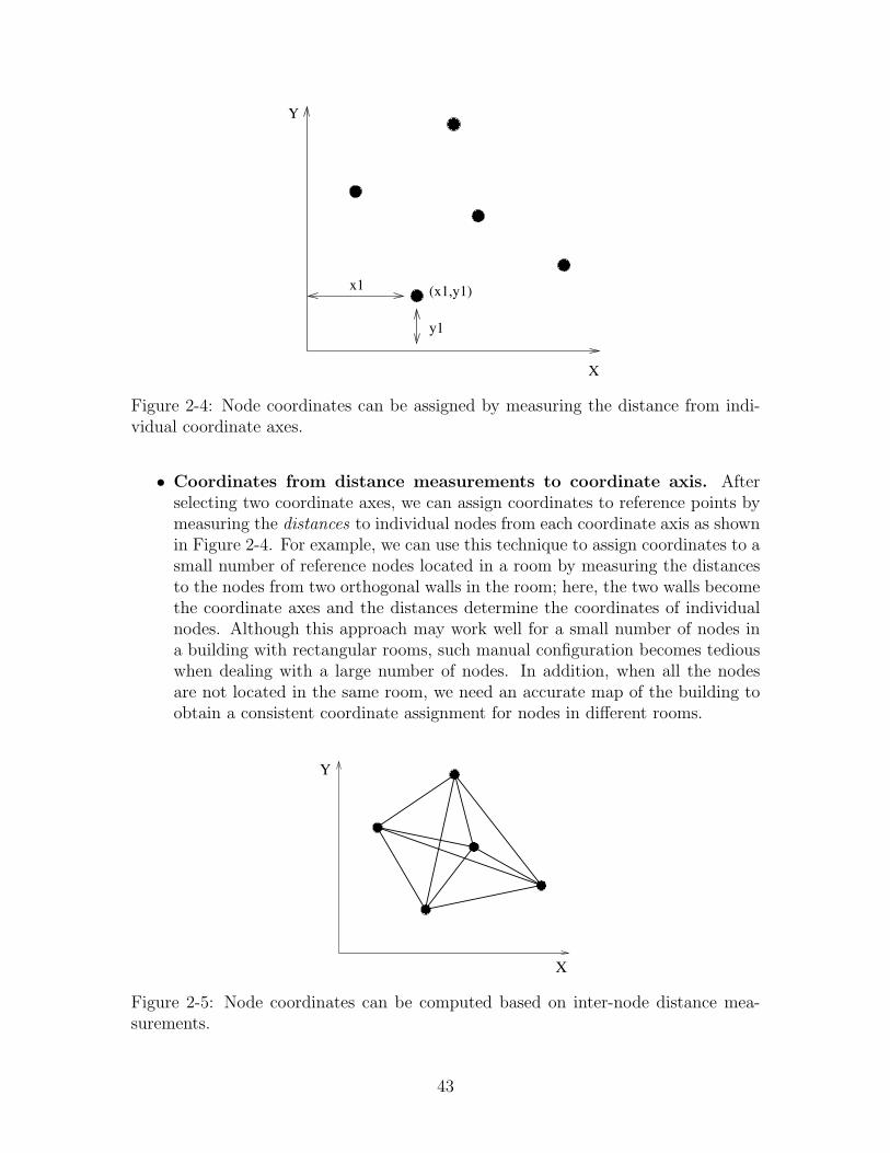
Figure 2-4: Node coordinates can be assigned by measuring the distance from indi-vidual coordinate axes.
• Coordinates from distance measurements to coordinate axis. Afterselecting two coordinate axes, we can assign coordinates to reference points bymeasuring the distances to individual nodes from each coordinate axis as shownin Figure 2-4. For example, we can use this technique to assign coordinates to asmall number of reference nodes located in a room by measuring the distancesto the nodes from two orthogonal walls in the room; here, the two walls becomethe coordinate axes and the distances determine the coordinates of individualnodes. Although this approach may work well for a small number of nodes ina building with rectangular rooms, such manual configuration becomes tediouswhen dealing with a large number of nodes. In addition, when all the nodesare not located in the same room, we need an accurate map of the building toobtain a consistent coordinate assignment for nodes in different rooms.
X
Y
Figure 2-5: Node coordinates can be computed based on inter-node distance mea-surements.
43
X
Y
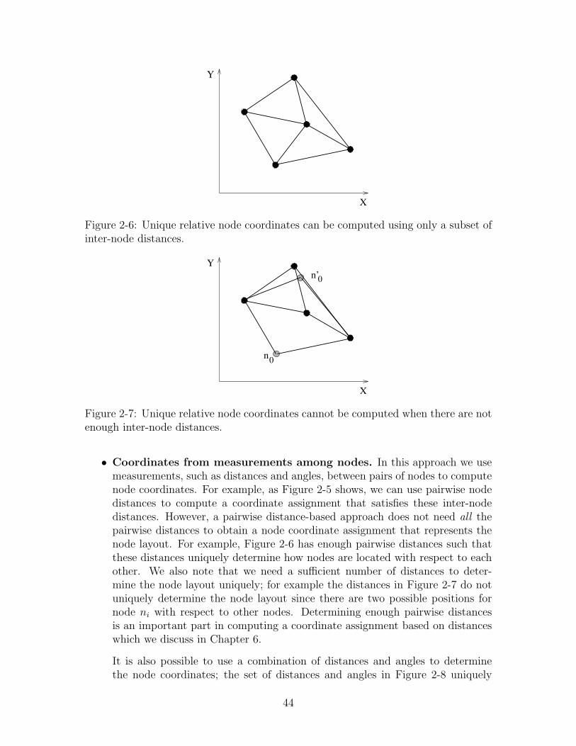
Figure 2-6: Unique relative node coordinates can be computed using only a subset ofinter-node distances.
n’
X
Y
n0
0
Figure 2-7: Unique relative node coordinates cannot be computed when there are notenough inter-node distances.
• Coordinates from measurements among nodes. In this approach we usemeasurements, such as distances and angles, between pairs of nodes to computenode coordinates. For example, as Figure 2-5 shows, we can use pairwise nodedistances to compute a coordinate assignment that satisfies these inter-nodedistances. However, a pairwise distance-based approach does not need all thepairwise distances to obtain a node coordinate assignment that represents thenode layout. For example, Figure 2-6 has enough pairwise distances such thatthese distances uniquely determine how nodes are located with respect to eachother. We also note that we need a sufficient number of distances to deter-mine the node layout uniquely; for example the distances in Figure 2-7 do notuniquely determine the node layout since there are two possible positions fornode ni with respect to other nodes. Determining enough pairwise distancesis an important part in computing a coordinate assignment based on distanceswhich we discuss in Chapter 6.
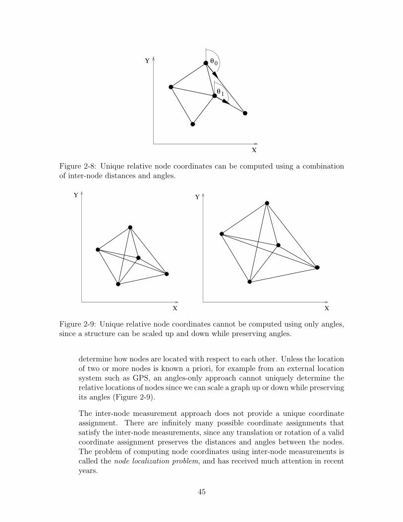
It is also possible to use a combination of distances and angles to determinethe node coordinates; the set of distances and angles in Figure 2-8 uniquely
44
X
Y
θ
θ0
1
Figure 2-8: Unique relative node coordinates can be computed using a combinationof inter-node distances and angles.
X
Y
X
Y
Figure 2-9: Unique relative node coordinates cannot be computed using only angles,since a structure can be scaled up and down while preserving angles.
determine how nodes are located with respect to each other. Unless the locationof two or more nodes is known a priori, for example from an external locationsystem such as GPS, an angles-only approach cannot uniquely determine therelative locations of nodes since we can scale a graph up or down while preservingits angles (Figure 2-9).
The inter-node measurement approach does not provide a unique coordinateassignment. There are infinitely many possible coordinate assignments thatsatisfy the inter-node measurements, since any translation or rotation of a validcoordinate assignment preserves the distances and angles between the nodes.The problem of computing node coordinates using inter-node measurements iscalled the node localization problem, and has received much attention in recentyears.
45
2.4.1 Anchor-based vs Anchor-free Localization Algorithms
Previous research has addressed different versions of the node localization problem.We characterize the algorithms developed to solve this problem in two different ways.The first characterization is based on whether or not the particular algorithm re-lies on anchor nodes, which are nodes with pre-configured coordinates. The secondcharacterization is based on whether the particular algorithm is an incremental or aconcurrent algorithm. Cricket uses an anchor-free, concurrent algorithm (Chapter 7).
• Anchor-based algorithms. Algorithms that rely on anchor nodes assumethat a certain number or a fraction of the nodes know their coordinates, e.g.,by manual configuration or using some other location system such as GPS. Thefinal coordinate assignment of the individual nodes will therefore be with respectsome other coordinate system that determined the coordinates of the anchornodes. A location system built around localization algorithms that need anchornodes has the limitation that it needs another location system to determine theanchor node positions, and cannot be applied when another location system isunavailable (e.g., inside a building). In practice, Anchor-based algorithms needa large number of anchor nodes for the resulting position errors to be acceptable(see Section 2.4.3).
• Anchor-free algorithms. Anchor-free algorithms use local measurements todetermine node coordinates, and do not assume the availability of nodes withpre-configured coordinates. For a given graph, a coordinate assignment ob-tained from an anchor-free localization algorithm will not be unique since thecoordinate assignment continues to be valid under translation and rotation.
2.4.2 Incremental vs Concurrent Localization Algorithms
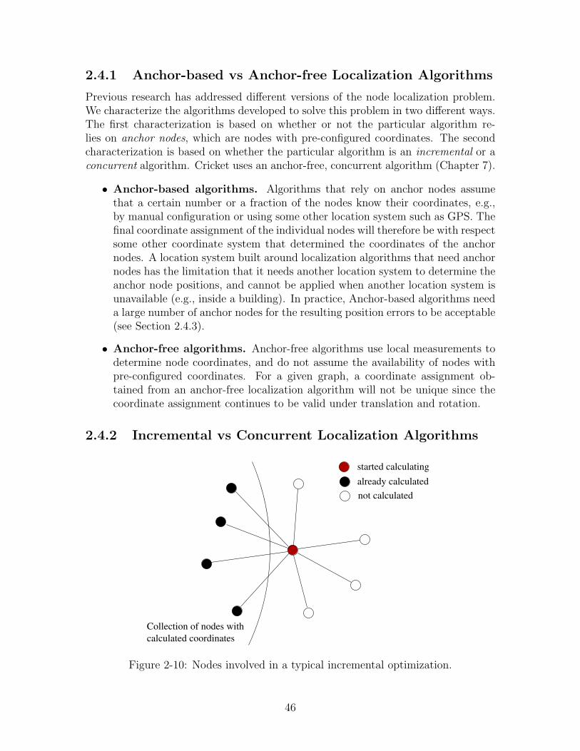
Collection of nodes withcalculated coordinates
already calculatedstarted calculating
not calculated
Figure 2-10: Nodes involved in a typical incremental optimization.
46
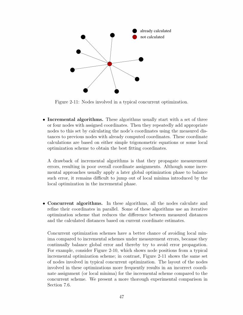
not calculatedalready calculated
Figure 2-11: Nodes involved in a typical concurrent optimization.
• Incremental algorithms. These algorithms usually start with a set of threeor four nodes with assigned coordinates. Then they repeatedly add appropriatenodes to this set by calculating the node’s coordinates using the measured dis-tances to previous nodes with already computed coordinates. These coordinatecalculations are based on either simple trigonometric equations or some localoptimization scheme to obtain the best fitting coordinates.
A drawback of incremental algorithms is that they propagate measurementerrors, resulting in poor overall coordinate assignments. Although some incre-mental approaches usually apply a later global optimization phase to balancesuch error, it remains difficult to jump out of local minima introduced by thelocal optimization in the incremental phase.
• Concurrent algorithms. In these algorithms, all the nodes calculate andrefine their coordinates in parallel. Some of these algorithms use an iterativeoptimization scheme that reduces the difference between measured distancesand the calculated distances based on current coordinate estimates.
Concurrent optimization schemes have a better chance of avoiding local min-ima compared to incremental schemes under measurement errors, because theycontinually balance global error and thereby try to avoid error propagation.For example, consider Figure 2-10, which shows node positions from a typicalincremental optimization scheme; in contrast, Figure 2-11 shows the same setof nodes involved in typical concurrent optimization. The layout of the nodesinvolved in these optimizations more frequently results in an incorrect coordi-nate assignment (or local minima) for the incremental scheme compared to theconcurrent scheme. We present a more thorough experimental comparison inSection 7.6.
47
2.4.3 Node Localization Algorithms
Moore et al. describes a three phase, anchor-free, algorithm to localize a collectionof mobile nodes [63]. During the first phase, nodes form clusters and each clustercomputes a local coordinate assignment using an incremental algorithm. During theoptional second phase, the coordinate assignment within each cluster is improvedusing a optimization scheme. The third phase of the algorithm stitches the clusterstogether to obtain a coordinate assignment for all the nodes within some local co-ordinate system. The use of robust quadrilaterals during the first phase makes thisalgorithm robust to measurement noise.
The ABC algorithm is an incremental algorithm that does not use anchor nodes [81].ABC first selects three in-range nodes and assigns them coordinates to satisfy theinter-node distances, and then incrementally calculates the coordinates of nodes us-ing the distances to the three nodes whose coordinates have already been calculated.This incremental scheme results in error propagation. The authors report that with5% range error, ABC results in about 60% average position error. This sort of cas-cading error is typical of many incremental algorithms.
Doherty et al. describe an anchor-based algorithm for localization using onlyconnectivity constraints among beacons [29]. They represent the connectivities as aset of convex position constraints, and use a centralized linear-programming algorithmto solve for the node positions. Moses et al. present a similar approach that usesa maximum-likelihood based centralized algorithm for sensor locations using rangeestimates to a number of fixed anchor nodes [64].
Bulusu et al. describe a GPS-less scheme that uses the radio connectivity of anode to a set of anchor nodes to determine its coordinates [12]. The coordinatesof the non-anchor nodes are obtained by calculating the centroid of all the anchorsin the nodes radio-range. This is a concurrent algorithm, but it does not use anyoptimization. In simulations, the authors report about 12% localization error withapproximately 12 anchor nodes per non-anchor node (R
d= 2 where R is the radio
range and d is the separation between anchors). In this scheme, the ratio of theanchor nodes to non-anchor nodes is rather large.
The Terrain algorithm, another anchor-based algorithm, builds on ABC [81]. Eachanchor starts the ABC algorithm. Using the coordinates assigned from ABC, eachnode calculates the distances to at least three anchors. Then, each node performsa concurrent optimization using the distances to the anchors and the anchor coordi-nates. The authors report about 25% position error (actual offset of the node positionfrom the true position) with 5% range error. They also mention that position errorsshow a high variance and may diverge during the optimization phase. A related algo-rithm for localizing nodes in an ad hoc network uses hop-count and radio strength asdistance measures, but assumes nearly uniform node density and no occlusion [66].
Savarese et al. describe a two-phase, anchor-based, concurrent, localization algo-rithm [82]. The first phase of the algorithm, Hop-Terrain, is a variant of Terrain, andis robust against ranging errors. The second phase is a simulated-annealing based op-timization. With 5% range errors, 10% of the nodes being anchors, and 12 neighborsper node, this algorithm results in about 12% average position error.
48
Savvides et al. describe an anchor-based collaborative multilateration [84]. Here,a node solves a set of over-constrained equations relating the distances among a set ofanchors and a set of non-anchor nodes (including itself). For a sample graph of 300nodes, the algorithm needs about 30 (10%) anchor nodes to calculate the location ofthe other nodes. Iterative multilateration, an incremental component of their algo-rithm, produces node position errors within 20 cm of a node’s actual positions, whenthe ranging error is small (2 cm, Gaussian-distributed). This experiment consists of50 nodes, with a 3 m ranging system, deployed in a square grid of 15 m × 15 m, andwith 10% of the nodes being anchors.
Niculescu et al. present an anchor-based, distributed algorithm that uses angle-of-arrival (AOA) for localization [67]. In this algorithm, nodes iteratively obtain positionand orientation information starting from anchor (landmark) nodes. One potentialproblem with this approach is that obtaining precise angle estimates is often difficult.
Howard et al.’s localization scheme uses robots equipped with odometric equip-ment moving through an environment to discover fixed location beacons [49]. Then,a spring-mass based optimization is used to obtain the final beacon coordinates. Theauthors mention the possibility of the optimization reaching a local minimum, but,also mention that this is a rare event. In Section 7.6.1, we show that spring-massbased optimization schemes with arbitrary initial coordinate assignments have a highprobability of reaching a local minimum. We believe that the use of a robot by theauthors to explore and discover the beacons resulted in an approximately “order cor-rect” (as explained in Chapter 7) initial coordinate assignment, which in turn reducesthe possibility of a local minima during the optimization phase.
Shang et al. discuss an anchor free centralized localization algorithm [88]. Theauthors propose a distributed version of the algorithm that first localizes regions ofthe network. Later these regions have to be “stitched” together. But the authors donot provide a distributed algorithm for stitching together pieces of the network; webelieve that developing such an algorithm is a significant undertaking.
Rao et al. use shortest-path hopcounts from a collection of nodes to computea coordinate assignment that approximates the physical layout of the nodes in agraph [75]. Caruso et al. describe a similar algorithm, which uses shortest-pathhopcounts from three elected nodes on the periphery of a isotropic graph, boundedby a convex polygon, to compute node coordinates [14].
Bulusu et al. study the performance characteristics of different RF-based beaconconfiguration algorithms and conclude that node density is an important determinantof performance [11]. This paper also contains a detailed survey of various beacon-based localization schemes.
Embedding a graph with given edge lengths also arises in the context of recon-structing the geometry of molecular structures in an area called distance geome-try [25]. In this context, distance measurements are substantially less accurate, andseveral techniques have been developed to refine estimates and reduce error boundsby combining several constraints. Berger et al. [8] give efficient algorithms for embed-ding a graph with error-prone edge lengths, even when nearly half of the edges mighthave completely inaccurate lengths. However, these algorithms rely on every nodehaving a constant fraction of the nodes as neighbors, for a total of Ω(n2) links between
49
n nodes; this is an unreasonable assumption for a typical indoor node deployment,where the average connectivity is much smaller than n− 1.
2.4.4 Mobile-Assisted Node Localization
Once Cricket beacons are deployed, we use a localization algorithm to compute acoordinate assignment that resembles the beacon layout in the space, based on inter-beacon distances. However, the beacons cannot obtain inter-beacon distances dueto the properties of the sensors used and the lack of line-of-sight between beacons.Chapter 6 describes how we use a mobile listener to obtain a sufficient number ofinter-beacon distances as input to the localization algorithm. Some previous workalso use measurements taken with a mobile node to compute the coordinates of a setof fixed nodes.
Scott and Hazas examine different approaches to determine fixed node positionsusing distance estimates at receiver nodes [87]. Their experiments include both dis-tances obtained at nodes mounted on a mobile frame and raw distances obtained byplacing multiple nodes on the floor or from a mobile carried by users. They reportbetter results using the mobile-frame based approach compared to the raw distanceapproach (however, the paper does not report the size of the fixed frame used). Inthe raw distance approach, they used simulated annealing to optimize the positionsof all the nodes in parallel, this sometimes lead inferior performance due to the pres-ence of local minima in the objective function. In contrast, we break the localizationproblem to two manageable pieces. We first determine the minimum number of nodesand samples needed per one small group to obtain inter-node distances within thisgroup. Our use of groups with small number of nodes reduces the possibility of localminima and the use of only the computed distances in localization phase makes thelocalization algorithm scalable with respect to the number of reference nodes.
Pathirana et al. uses RF signal strength measurements collected at a mobilerobot to localize RF beacons [69]. They use RF signal strength to determine distancebetween the robot and fixed beacons. The use of the mobile robot improves theaccuracy of RF signal strength based distance measurements, since signal strengthvariations due to spatial fading of RF signals may be reduced. They assume theavailability of precise velocity and acceleration of mobile robot to compute the positionof the robot within a local coordinate system as the robot collects data. Our approach,although uses data collected at a mobile listener, does not assume any knowledge ofthe location of the mobile listener during the data collection process.
Corke et al. use a flying robot equipped with a GPS receiver to localize stationarynodes [21]. The robot beams down its current GPS coordinates using RF; and thestationary nodes use this information to compute their position. In contrast to ourapproach, this scheme also assumes that the location of the mobile node is known.
Sichitiu and Ramadurai use a GPS equipped mobile node to localize fixed receivernodes [90]. They use the RF signal strength to represent the distance between themobile node and fixed nodes. Again the assumption of availability of mobile nodelocation makes their approach different from our mobile assisted approach.
50
2.5 Orientation Measurement
Orientation is another form of location information that is useful for developinglocation-aware applications. The two main techniques for obtaining orientation are:orientation from earth’s magnetic field, and orientation from gyroscopes.
2.5.1 Orientation from the Earth’s Magnetic Field
The Earth acts as a giant magnet because of the electric currents generated by themovements in its core [38, 93]. The orientation of a given direction can be obtainedfrom the orientation of the Earth’s magnetic poles with respect to that direction; thisprinciple forms the basis of operation of the magnetic compass. A freely suspendedmagnet, in the absence of any stray magnetic fields, aligns itself along the magneticpoles of the Earth. Since ancient times, this property has been used to build magneticcompasses for navigation [2].
Although the location of the earth’s magnetic poles are assumed to be fixed (withrespect to the earth) for most practical purposes, recent studies have shown thatearths magnetic poles are drifting while in some regions the poles have even flippedover [53, 50]. It is also known that the directions of the Earth’s magnetic field reversesover a long time scale. The biggest drawback of magnetic compass is the variation ofEarth’s magnetic field due to ferrous metals such as iron and steel in the environment.The performance of a magnetic compass is also affected by stray magnetic fieldscaused by various electrical equipment. Because of these shortcomings, they do notperform well in many indoor environments. For instance, when used inside a ship, itis necessary to make corrections to the compass to offset the effects due to ship’s steelbody. However, such corrections become impractical when the compass is mobilewith respect to the surroundings.
A fluxgate compass also determines orientation from the orientation of the earth’smagnetic field. However, unlike a mechanical magnetic compass, a fluxgate compassoperates by measuring the Earth’s horizontal magnetic field using a toroid or a coil.
Similar to fluxgate compasses, electronic compasses use sensors to measure theearth’s horizontal magnetic filed. However, instead of a toroid, these use either Hall-effect sensors or Magnetoresistive sensors to measure Earth’s magnetic field [47].
2.5.2 Orientation from Gyroscopes
Gyroscopes use a dead-reckoning technique to keep track of the orientation of anobject. The gyroscope is first initialized with a known orientation. After the initial-ization, the gyroscope keeps track of the changes in the object’s orientation in 3Dspace to determine the current orientation of the object with respect to the originaldirection. Being a dead-reckoning approach, the gyroscopes suffer from accumulationof error.
There are several types of gyroscopes for measuring orientation. A gyrocompassuses a fast spinning wheel mounted on a platform that allows the wheel to freelyrotate in 3D. Since a spinning wheel try maintain a fixed orientation, the spinning
51
wheel retains its original orientation as the object containing the platform rotates in3D. Since the spinning wheel maintains its original orientation, the objects orientationcan be obtained from the offset between the current orientations of the object andthe spinning wheel.
In fiber-optic gyroscope, light emitting from a laser diode travels along two fiber-optic cables wound in opposite directions. The phase difference between the lightexiting the fiber-optic cables depends on the distances the light traveled along thetwo cables. When the two windings are rotated around their axis, the distances thelight travel along the two windings change, and the angle of rotation reflects itself asa change in the measured phase difference. To determine rotation in 3D, three setsof windings, placed perpendicular to each, are used.
2.6 Chapter Summary
This chapter examined the general principles underlying the design of location sys-tems. This chapter also described various indoor and outdoor location systems, re-lated work on node localization, and systems for obtaining orientation information.The next chapter describes the architecture of the Cricket system.
52
Chapter 3
Cricket System Architecture
This chapter describes the architecture of the Cricket system. Section 3.1 describesthe different components of the Cricket architecture and how they inter-operate. Sec-tion 3.2 describes the main software components of the Cricket system. Section 3.3describes the Cricket hardware design and implementation.
3.1 Cricket System Architecture
Each node in the Cricket system is a small hardware platform consisting of an RFtransceiver, a microcontroller, and other associated hardware for generating and re-ceiving ultrasonic signals and interfacing with a host device (Figure 1-4). There aretwo types of Cricket nodes: beacons and listeners. Cricket beacons act as fixed ref-erence points of the location system and are typically attached to the ceiling andwalls of a building, while Cricket listeners are attached to objects that need to obtaintheir location. Each beacon periodically transmits a radio frequency (RF) messagecontaining beacon-specific information, such as the unique beacon-ID, the beaconcoordinates, the physical space associated with the beacon, etc. At the start of theRF message, a beacon transmits a narrow ultrasonic (US) pulse that enables lis-teners to measure the distances to the beacons using the difference of arrival timesof RF and ultrasonic signals. To reduce beacon power consumption and ultrasonichardware complexity, this ultrasonic pulse does not carry any data. Cricket listenerspassively listen to beacon transmissions and compute distances to nearby beacons.Each listener uses these distances and the information contained in the beacon RFmessages to compute their space position and orientation (or some subset of thislocation information).
Each beacon is configured with its “space”, a human-readable text string. Whenbeacons are deployed, they do not know their position coordinates. To computebeacon coordinates, a Cricket listener attached to a mobile platform roams around andcollects distances from the beacons to itself. Using these distances, a host attachedto the listener computes inter-beacon distances; the roaming mobile platform collectsenough distances such that the set of computed inter-beacon distances uniquely definehow the beacons are located with respect to each other. Next, the host uses these
53
inter-beacon distances to compute a beacon coordinate assignment that resembles thetrue beacon embedding.
Distance estimation using coupled RF and US signals enables accurate measure-ment of beacon-to-listener distances. Since the listeners do not actively transmitmessages, the performance of the system is independent of the number of listenersin the environment. As a result Cricket scales well with respect to the number ofusers and objects that need location information. Since listeners only passively listento beacon transmissions to determine their location, the position of a user carryinga listener is not tracked by the Cricket system, which enables location-aware appli-cations without compromising user privacy; at the same time, it is possible to buildtracking applications to track the position of a rapidly moving object by “inverting”the roles of the beacons and the listeners. Since a beacon coordinate assignment canbe computed with only limited manual intervention, the Cricket system is easy todeploy and configure.
3.2 Cricket Software Architecture
The Cricket software architecture consists of two parts: the software running on theattached host, and the firmware running on the Cricket beacon and listener.
Unique ID Space ID Beacon (x , y , z)coordinates Temperature
Figure 3-2: The Cricket beacon message format.
Figure 3-1 shows the block diagram of the Cricket beacon firmware. One softwaremodule on the beacons schedules beacon RF and ultrasonic message transmissions,while another module exposes an configuration API over the serial RS 232 interface.This API is used to set and read various parameters such as the average beaconing
rate. The beacon RF message contains the following information: a unique identifier,a space identifier (the name of the space the beacon is located in), beacon coordinates,and the measured ambient temperature at the beacon (Figure 3-2).
The listener firmware consists of three modules as shown in Figure 3-3. Thelistener distance measurement module uses the timing of RF and US arrival events tomeasure distances to nearby beacons and also implements the interference detectionalgorithm described in section 4.1. The listener also contains a configuration module,which exposes an API over the serial RS 232 interface, similar to the beacon. Thedistance store submodule keep track of recently heard beacons and the distances tothese beacons; this submodule also implements the “MinMode” algorithm describedin section 4.1. The distance store module exposes an API that reports distances tonearby beacons according to the current listener configuration.
Listener Interface (cricketd)
Processor (CricketDaemon)
Java Applications (Clientlib)
Figure 3-4: Cricket host software architecture.
3.2.2 Cricket Serial Configuration API
The serial configuration API enables the reading and setting of the values of variousparameters in the beacons and listeners. This API is inspired by the Hayes ATcommand set for modems [4]. To issue these commands, the beacon or the listener
55
ServerBrokerObject
Object 1 Object 2 Object N...
Callback
Commands
CricketDaemon
TCP/IPJava App
Figure 3-5: Clientlib Architecture.
must be attached to an RS232 serial interface configured as follows:
Transmission speed 115200 bits/secondData format 8 bits, no parityFlow control Xon/Xoff (“software”)
Stop bits 1
Once the beacon or the listener is attached to a host, these commands can beissued using a standard serial port utility such as HyperTerminal or minicom. Thecommand format is:
<directive> <command> <parameters>
〈directive〉 “G” for “get” and “P” for “put”.<command> The command.<parameters> The argument(s) to the command.
In response to a command, the Cricket listener or beacon echoes the commandfollowed by the result:
<command> <result>
A complete description of the commands and their parameters are described in theCricket user manual available from the Cricket Web site (http://cricket.csail.mit.edu).
56
3.2.3 Cricket Host Software
Figure 3-4 shows the block diagram of the Cricket host software that runs on theattached host. The CricketD daemon connects to the serial port and exposes theCricket serial port API described above. This daemon listens on a TCP port (2947),and applications can access the Cricket serial API by opening a TCP connectionto this port. The CricketDaemon connects to CricketD using a TCP connection.CricketDaemon processes raw distance data from CricketD and computes the lis-tener space and position. Applications can access CricketDaemon through a TCPport (5001). The Clientlib Java library provides support to build location-awareJava applications (Figure 3-5). This library is composed of a ServerBroker ob-ject that connects the CricketDaemon to obtain current location information. TheServerBroker exports a callback interface. Various Java objects register with theServerBroker to be notified whenever the device’s location changes. During regis-tration, these objects use a bit-mask to specify which specific location change eventsthey are interested in (e.g. the current space, position, etc.).
3.3 Hardware Implementation
MicrocontrollerAtmega 128L
AmplifierR
UltrasonicReceiver
AmplitudeDetector
RS 232 Driver
RS 232 Connector
Vcc
3 V
T
UltrasonicTransmitter
Ultrasonic Driver (12V)
VoltageMultiplier
418 MHz
Mica Mote interface
RF Transceiver
Temperature Sensor
7.37 MHz32.77 kHz
−
+
Figure 3-6: Cricket hardware implementation. The beacon and the listener devicesare identical.
The hardware implementations of the Cricket beacon and listener are identical.Figure 3-6 shows a block diagram of the Cricket beacon and listener hardware. Fig-ure 3-7 shows the placement of the important components in the hardware implemen-tation.
The Cricket hardware implementation has the following submodules (a completehardware schematic is in Appendix A).
57
Figure 3-7: Cricket hardware components and layout.
• Microcontroller. Cricket uses an Atmega 128L microcontroller operating at7.3728 Mhz when active [5]. The microcontroller uses a 32.768 kHz clock fortiming during the sleep mode. The Atmega128L is a 8-bit processor with 8kBytes of RAM 128 kBytes of FLASH ROM (program memory), and 4 kBytesof EEPROM (as mostly read-only memory). The microcontroller operates atabout 3 V and draws about 8 mA and 8 µA in the active and the sleep modesrespectively.
• RF transceiver. The CC1000 RF transceiver used in Cricket is configuredto operate at 433 MHz [16]. This transceiver uses Manchester encoding andFrequency Modulation (FM) [57]. In Cricket, the transceiver is configured tosend and receive data at a rate of 19.2 kilobits/s.
• Ultrasonic transmitter. The ultrasonic transmitter submodule drives a 40kHz piezo-electric open-air ultrasonic transmitter at 12 V [102]. Under softwarecontrol, this submodule generates ultrasonic pulses of duration 125 µs. Thevoltage multiplier module generates 12 V from the 3 V supply voltage to drivethe ultrasonic transmitter.
• Ultrasonic receiver. We use an open-air type piezo-electric sensor that op-erates at 40 kHz to detect ultrasonic signals. The output of this sensor isconnected to a two-stage amplifier with a programmable voltage gain between70 dB and 78 dB. The ultrasonic signal is detected when the amplifier outputgoes above a preset threshold.
• Expansion connector. The Cricket node includes a connector that is pin-compatible with the Mica mote sensor interface. Mote-compatible sensor boards
58
can be connected to this board to build location-enhanced sensor networks. Itis also possible to attach Mote processor boards to the Crickets for increasedprocessing power. This connector can also be used to connect Cricket compassboards for obtaining listener orientation.
• RS 232 interface. An RS 232 interface with a DB-9 connector is used toattach a host device to the Cricket node.
• Temperature sensor. A pre-calibrated thermistor-type temperature sensorenables the beacons and the listeners to measure the ambient temperature tocompensate for variations in the speed of sound with temperature.
• Unique ID. An 8-byte hardware ID, which is similar to an Ethernet MACaddress, uniquely identifies every Cricket node.
3.3.1 Powering the Beacons and Listeners
Each Cricket node may be powered using two AA batteries, a power adapter, or solarcells.
Since beacons periodically transmit location information, they need a power sourcethat can last for a sufficiently long time. A beacon consumes about 2.2 mA current onaverage and can operate on two AA batteries for five to six weeks. We have success-fully powered the beacons using solar cells placed next to indoor lighting. A possiblesolution to reduce beacon power consumption is to use a low-power wake-up mecha-nism to wakeup the beacons when a nearby listener needs location information [89].
3.4 Chapter Summary
This chapter described the Cricket system architecture. This chapter also describedthe software and hardware architecture of Cricket.
The next chapter describes and evaluates the techniques for obtaining accuratebeacon-to-listener distances in Cricket.
59
60
Chapter 4
Distance Estimation in Cricket
Cricket listeners use distance measurements to nearby beacons to compute listener lo-cation. Since typical indoor applications require accurate location information, listen-ers must be able to measure these distances accurately. Since beacon transmissions inCricket are not centrally coordinated, the distance measurement technique also needsdeal with possible interference among multiple beacon transmissions This chapter de-scribes the techniques, algorithms, and the hardware and software implementationsused in Cricket to obtain accurate beacon to listener distances. Section 4.1 describesthe use of time-difference-of-arrival (TDOA) of RF and ultrasonic (US) signal to com-pute distances. This section also describes how various environmental factors affectthe distance measurements, and examines Cricket’s distance measurement accuracy.
The lack of centralized beacon coordination causes transmissions from differentbeacons to interact at the listener, resulting in incorrect distance samples. Section 4.2describes how Cricket handles these incorrect samples using a combination of threealgorithms: interference avoidance at the beacons, interference detection at the lis-tener, and history-based filtering. Section 4.3 examines the throughput of a networkof Cricket Beacons, in terms of both beacon transmission rate and the distance samplerate at the listener, using simulations and real-world experiments. We observe thatperiodic RF transmissions from a large number of deployed beacons cause scalabilityissues. Section 4.4 examines the scalability of the Cricket system by measuring therate of RF collisions due to imperfect RF carrier sensing and by studying the im-munity of the RF listeners to the interference from weak transmissions from far-offbeacons. Finally, we describe the hardware implementation of Cricket beacons andlisteners, and discuss various system deployment issues that arise in practice.
4.1 Distance Measurement from TDOA of RF and
Ultrasound
Cricket uses the TDOA of RF and US signals to measure beacon-to-listener distances.Cricket beacons periodically transmit an RF message containing beacon specific in-formation such as a unique identifier, coordinates, space ID, and measured ambienttemperature. At the start of each message, each beacon transmits a narrow ultrasonic
61
pulse.Since the velocity of RF is much larger than the velocity of sound, the US signal
lags behind the RF signal as the two signals propagate. When a listener receivesan RF message from some beacon, followed by an US signal, it measures the timeinterval δT between the start of the RF message and the arrival of the US signal atthe listener. The listener can compute the distance d to the beacon from:
δT =d
vus
− d
vrf
.
At normal room temperature and humidity, the speed of sound, vus ' 344 m/s, andspeed of light, vrf ' 3× 10⁸ m/s. Since vRF vUS,
d ' δT · vus
To reduce power consumption and to keep the hardware simple, the US signal is onlya narrow pulse that does not carry any data.
Because RF receivers take varying amounts of time to detect a valid preamble thatprecedes the actual RF message, the ultrasonic signal is transmitted at the start ofthe RF message rather than at the start of the RF signal itself; the receiver computesthe time interval δT between the start of the RF message and the detection of theultrasonic signal. The accuracy of the distance measurement depends both on theaccuracy of measuring the time interval δT , and the accuracy of the estimated speed ofsound used for distance computation. The accuracy of δT in turn depends on systemparameters such as the RF bit rate, ultrasonic sensors and the detection circuits, andthe timer resolution, while the speed of sound depends on environmental factors suchas ambient temperature, humidity, and atmospheric pressure.
4.1.1 Environmental Effects on the Speed of Sound
The speed of sound in air depends on environmental factors such as temperature andhumidity. In completely dry air with no humidity, the speed of sound (in meters persecond) depends only on the absolute temperature T (in Kelvin), and is given by [58]
vUS = 20.05√
T .
However, indoor air contains varying amounts of water vapor; with non-zero hu-midity, the speed of sound depends on the temperature, the relative humidity, andthe atmospheric pressure. Lord, using work by Cramer and Davis, presents a moreaccurate equation for calculating speed of sound under varying environmental condi-tions [94, 23, 27]. The speed of sound is not very sensitive to relative humidity andatmospheric pressure variations. For instance, at 25 0C and 101.325 kPa (atmosphericpressure at sea level), the speed of sound changes by only about 0.5% as the relativehumidity changes from 0% to 100%. At 25 0C and 50% relative humidity, the speed ofsound changes by only about 0.6% as the atmospheric pressure changes from 101.325kPa to 30 kPa (the atmospheric pressure at the top of Mount Everest). In contrast,
62
θ
θ
d
Beacon
Listener
Figure 4-1: Experimental setup to determine the Cricket distance measurement per-formance.
the speed of sound changes by ' 0.18% per 0C at 25 0C. Since the speed of sound hasa relatively large sensitivity to temperature variations, and since indoor temperaturecan easily vary by even 10 0C within the same room, we use temperature sensors onCricket beacons and listeners to compensate for changes in speed of sound due totemperature variations.
Each Cricket beacon measures the ambient temperature using an on-board tem-perature sensor, and includes this temperature in its RF message. When a listener Lcomputes its distance to a beacon B, the listener measures its temperature tL, anduses the value (tL + tB)/2 to represent the room temperature and computes the cor-responding speed of sound. The cricket nodes can measure the ambient temperaturewith an accuracy of ±10C.
4.1.2 Distance Measurement Performance
We used the following experimental setup to measure Cricket’s distance measurementaccuracy. We deployed a transmitter and a receiver as shown in Figure 4-1; this setupmimics a beacon mounted on the ceiling, and a listener held parallel to the ground.Figures 4-2 and 4-3 show the error between the measured distance and the truedistance for different values of d and θ. Each data point on the graph representsthe mean absolute error, calculated over 100 samples; the vertical bars representthe minimum and maximum absolute error within the 100 samples. Because theultrasonic sensors are not omni-directional, we could not get distance measurementsfor (d, θ) combinations that do not have a corresponding data point. We performedthe experiment in a controlled environment to prevent outlier distance measurementsdue to reflected ultrasonic signals.
We observe that the absolute measurement error increases with the beacon tolistener distance d. This increase is to be expected since increasing d causes thereceived US signal strength at the receiver to drop, causing the detection circuitsto take a longer time to detect the signal, resulting in an increased positive error.The ultrasonic transmitter and receiver radiation pattern shown in Figure 4-4 (from
63
0
20
40
60
80
100
120
-80 -60 -40 -20 0 20 40 60 80
Err
or (c
m)
Angle (degrees)
2 m4 m6 m8 m
Figure 4-2: The distance measurement error as a function of the angle of rotation (θin Figure 4-1) of the transmitter and the receiver at different transmitter to receiverdistances.
0
5
10
15
20
-80 -60 -40 -20 0 20 40 60 80
Err
or (c
m)
Angle (degrees)
2 m4 m6 m8 m
Figure 4-3: Zoomed-in version of Figure 4-2, showing the distance measurement erroras a function of the angle of rotation (θ in Figure 4-1) of the transmitter and thereceiver at different transmitter to receiver distances.
64
Figure 4-4: The radiation pattern of the Cricket ultrasonic transducer on a plane alongits axis in (r, θ) polar coordinates. The r represents the signal strength (sensitivity)in dB and the θ represents the offset from the Z axis of the transducer.
the manufacturer’s specification) explains the increase in error with increasing θ.As the radiation pattern shows, the transmitter and receiver sensitivity drops alongdirections that are away from the direction facing the ultrasonic transducer, hencewith increasing θ. With increasing θ, the received signal strength at the listenerdecreases, again resulting in increased error. We observe that Cricket has a rangingaccuracy of about 0.5% when the beacon and the listener are 2 m apart and are facingeach other; however, the ranging performance degrades as we increase the separationand when they do not face each other. For θ in the range (−40o, 40o), the error isunder 5 cm. We also observe that for large angles, for example θ = 90o, there areno data points, because the ultrasonic signal at the listener is too weak to detect atlarge angles. A listener cannot measure distance to a coplanar beacon, when both thebeacon and the listener are facing away from the plane, since this represents a θ of90o. Coplanar beacons, for instance when all the beacons are attached to the ceilingof a room, cannot measure inter-beacon distances although they can both transmitand receive RF and US signals.
4.1.3 Sources of Error in Distance Measurement
This section describes the possible sources of error when measuring distance betweena beacon and a listener.
• Environmental factors. As we described in Section 4.1.1, dependency of velocityof sound on environmental factors such as temperature, humidity, and atmo-spheric pressure causes errors in velocity of sound-based distance measurements.Although it is possible to reduce these effects by measuring these environmentalfactors and compensating for them, it is not possible to completely eliminate
65
RF A RF B US B US A
timet
Figure 4-5: Inaccurate distance estimate caused by a listener using RF (RFA) andultrasonic (USB) messages from different beacons to compute a distance estimate.
these effects since these factors can have different values along the path thesound travels.
• Lack of line-of-sight. If there is no line-of-sight path between the beacon andthe listener, the sound may reach the listener after bending over an edge (re-fraction) or after reflecting off of some object. Both refraction and reflectioncause the sound to travel a longer distance than the Euclidean distance betweenthe beacon and the listener, resulting in distance measurement errors.
• Errors in detecting US. Cricket uses a threshold based approach to detect thearrival of the US signal. Cricket listener detects the arrival of a US signal whenthe signal amplitude at the output of the US amplifier circuit reaches a presetthreshold (65 mV). However, the time taken for the received signal to reachthis threshold is dependent on the received signal strength (as evident fromSection 4.1.2). Hence, there is a received US signal strength dependent error inthe distance measurement.
• Timing quantization. In TDOA based distance measurement, a measured timeinterval is converted in to a corresponding distance. This time interval measure-ment involves two types of quantization errors. First, measurement of time hasa quantization error equal to the period (' 1 µs in Crickets) of the clock usedfor timing. Second, TDOA based approaches first detects the time of arrivalof some reference signal, usually RF, to start the time interval measurement;detecting the arrival the RF message has a quantization error equal to the RFbit duration (' 52 µs in Cricket).
• Variable interrupt service routine delays. As described previously, RF and USbased distance estimation requires the detection of RF arrival time. In Cricket,this detection is done within an Interrupt Service Routine (ISR) that handlesthe arrival of data form the RF transceiver. The invocation of this ISR canhave a variable delay due to the presence of competing ISRs. This results in anerror in the TDOA measurement.
• Arithmetic quantization. There can be quantization errors in the arithmeticroutines that convert TDOA measurements to corresponding distances.
66
RF A US B US A
time
Figure 4-6: In US interference, a foreign US signal (USB) arrives between the startof the RF (RFA) and US (USA) signals from some beacon A at a listener.
US A
time
RF A RF B
Figure 4-7: In RF interference, a foreign RF signal (RFB) arrives between the startof the RF (RFA) and US (USA) signals from some beacon A at a listener.
4.2 Preventing Beacon Interference
While Cricket has the attractive property that the collection of decentralized bea-cons is easy to configure and manage, the absence of explicit coordination of beacontransmissions can cause signals from different beacons to interfere at a listener, re-sulting in incorrect distance measurements. Consider the RF signals RFA and RFB,and the US signals, USA and USB, of two beacons A and B received at a listenerL. The signals RFA and RFB carry beacon specific data that enable L to identifytheir origins. In contrast, since the US signals in Cricket do not carry any data, Lcannot differentiate between the signals USA and USB. With no coordination amongbeacons, the signals from A and B can interfere at L as shown in Figure 4-5. HereUSB arrives immediately after RFA, but before the arrival of USA. Since L cannotdifferentiate between USA and USB, it would use the time difference t between RFA
and USB to calculate the distance to A, resulting in an incorrect distance sample.
Before we discuss how to prevent these incorrect samples, we identify two possibletypes of interferences. A foreign RF signal arriving between the RF and US signalsfrom a beacon A, as shown in Figure 4-7, is called an RF interference, while a for-eign US signal arriving between these signals (Figure 4-6) is called US interference.Combinations of these two types of interference are also possible.
We use a combination of three techniques to minimize, detect, and filter out theseincorrect distances caused by foreign signals in Cricket. We first set the system’sparameters to ensure that the RF range between a beacon and a listener is alwaysgreater than twice the US range. Under this assumption, we use a beacon schedulingalgorithm that minimizes beacon interference, and an interference detection algorithmat the listeners to detect remaining interference. However, since we cannot makehard guarantees about indoor RF propagation, there can be instances where ourassumption on the RF and US ranges fail. To deal with these situations, we usefiltering algorithms that examines the history of distance samples to filter out theremaining incorrect distance samples.
It must be noted that interference avoidance in Cricket is different from interfer-
67
ence avoidance in traditional communication systems such as wired Ethernet, sinceCricket uses two signals with different propagation characteristics, while traditionalinterference avoidance deals with only one signal. Before we discuss the interferenceavoidance algorithms in detail, we examine the salient characteristics of indoor RFand US signal propagation.
4.2.1 Indoor RF Propagation Characteristics
Cricket uses 433 MHz RF signals for transmitting location information. In free space,RF signals attenuate with the distance; since the RF signal strength at a receivershould be larger than some threshold for successful reception, there is some RF“range” beyond which a given transmitter and a receiver cannot communicate. In-building RF propagation is a well-researched topic, with most research concludingthat, for indoor environments, RF signal strength and RF connectivity has no welldefined correlation with the distance between the RF transmitter and the receiver.This lack of correlation is mostly due to the reflection and attenuation of RF signalsby metallic objects [76].
Indoor RF signal propagation is subject to attenuation similar to the free spaceattenuation of RF signals, although the exact attenuation profile is not predictable. Inthe absence of wave guides (which are specially designed metallic tubes that enablesRF signals to travel longer distances by repeated reflections), in-building RF rangeis typically less than the free-space range due to attenuation by various metallic andnon-metallic obstacles. Apart from attenuation with distance, there are also localvariations of RF signal strength due to destructive and constructive interference ofsignals reflected off of metallic objects (RF multipath effects). In general, we canprovide almost 100% RF coverage inside a room by using an RF transmitter withhigh enough transmit power. However, as we increase the RF transmit power toachieve high coverage within a room, there will be significant RF leakage outside theroom as well.
4.2.2 Indoor US Propagation Characteristics
US signals, at the frequency used by Cricket (40 kHz), do not penetrate physicalobjects such as walls. Since the wavelength of the US signals is smaller than thewavelength of the human audible sound, the ultrasonic signals do not diffract atopenings such as doorways as readily as audible sound. Hence, the ultrasonic signalsstay mostly confined inside an enclosed areas such as a room with only a limitedleakage through openings such as doorways.
Figure 4-8 shows the physical construction of the US transmitters and receiversused in Cricket [102]. Since the construction of these transmitters and receivers issymmetrical about the Z axis, we assume that these transmitters and receivers havean omni-directional radiation pattern on the X − Y plane. Figure 4-4 shows a (ρ, θ)polar plot of the radiation pattern of these transducers on a plane perpendicularX − Y plane, going through the Z axis. Here, the r value represents the the signalstrength (sensitivity) in dB and θ represents the angle offset from the Z direction.
68
X
Y
Z
Connector A Connector B
Plastic Base
Piezo Disk
Metal Cone
Figure 4-8: The internal construction of the ultrasonic transmitters and receivers usedin Cricket. The two connectors A and B are attached to the top and the bottom ofthe piezo electric disk. The thickness of the piezo electric disk depends on the polarityand the magnitude of the voltage applied across these connectors. The dimensions ofthe piezo material causes the disk to resonate at 40kHz.
The figure shows that these transmitters and receivers have the highest sensitivityin the direction of the Z axis and the sensitivity drops as we move away from theZ axis. For example, the sensitivity drops to 1% (−20 dB) of the maximum at±50o away from the Z direction. When an ultrasonic transmitter is attached to theceiling of a room with the transmitter facing down, the received signal strength is amaximum when a receiver is located directly under the transmitter (θ = 0). As thereceiver moves away from the transmitter in a lateral direction, the received signalstrength drops due to the combined effects of increased transmitter-receiver distanceand due to the radiation pattern. This decay of ultrasonic signal strength results ina well-defined coverage area for a ceiling-mounted transmitter. Similar to RF, thesize of this coverage area depends on the transmit signal strength and the receiversensitivity. Since ultrasonic signals are easily reflected off of hard surfaces such aswalls, a listener could receive a given ultrasonic transmission from multiple paths.Consider an ultrasonic transmission reaching a receiver along two paths: the directpath from the transmitter to the receiver (P1), and a path where the signal getsreflected off an obstacle such as a wall (P2). Let these path lengths be l1 and l2respectively. For a given transmission, the time gap δt between the arrival of signalsalong these paths at the receiver is given by:
δt =l2 − l1
vus
In an indoor environment, the value l2 − l1 can be several meters, causing δt to beseveral milliseconds long. For example, if l2− l1 = 2 m, δt ' 6 ms. Because of reflec-tions, a single transmitted wavefront causes a series of received signals with differentdelays, usually resulting in a wide pulse—with a duration of several milliseconds—at
69
Ultrasonic coverage area
RF coverage area
Figure 4-9: Although indoor propagation of RF and US is not predictable, we canensure that RF range > 2 × US range most of the time by increasing the RF trans-mission power as necessary. The inability of US signals to permeate obstacles alsotends to reinforce this relationship.
the receiver.
At a speed of vus, the ultrasonic signal travels a distance d within a time d/vUS.If the ultrasonic transmitter and the receiver have a maximum range of Rus, theultrasonic signal can travel for time at most Rus/vus. If the duration (width) ofthe ultrasonic transmission is tus, the ultrasonic signal must “disappear” within timeDus = Rus/vus + tus. With Rus ' 10 m and tus = 250 µs, an ultrasonic transmissionfrom a Cricket beacon completely dies down after about 30 ms.
4.2.3 Interference Avoidance Algorithm at the Beacons
Since both RF and US transmissions have a limited range, and since we can increasethe RF range by increasing the RF transmission power as necessary, we can setthe RF transmission power such that RF range, Rrf and US range Rus satisfy thecondition Rrf > 2 × Rus with high likelihood (we cannot guarantee a probability of1 due to localized variations of RF signal strength arising from multipath effects).As Figure 4-9 shows, the inability of US signals to penetrate obstacles reinforces thisrelationship.
We observed that the US signals from a given beacon transmission disappearwithin an interval DUS; the duration of the beacon RF message is made smaller than
70
while true dor ← randomUniform(T1,T2);delay(r);startRF Rx();delay(Dus);if no beacon message and RF carrier free then
Dus. Since both RF and US signals from a beacon transmission cease to exist afterDus, the signals from two beacon transmissions that are separated by more than Dus
cannot interfere at a listener.We use the beacon transmission scheduling algorithm shown in Figure 4-10 to
minimize interference among beacons that are within RF range, by separating theirtransmissions by at least Dus. Each beacon sleeps for some random interval r; next,before transmitting an RF signal, the beacon turns on its RF receiver and waits forDus to see if it hears a beacon message within this interval; if it does not hear anybeacon message within Dus, the beacon transmits its own beacon message after RFcarrier sensing to ensure that there are no ongoing beacon transmissions. It must benoted that, during the Dus period, the beacon specifically checks for beacon messagesbut ignores other message types.
This algorithm ensures that, under perfect carrier sensing (where a beacon candetect all the ongoing RF transmissions from other beacons within its range beforestarting its own transmission), RF messages from two beacons within each others RFrange are separated by at least DUS. The relationship RangeRF > 2 × RangeUS,guarantees that if some listener is within the US range of two beacons, then thosetwo beacons must be within each other’s RF range. Since transmissions from beaconswithin each other’s RF range are separated by at least Dus, this scheduling algorithmprevents US interference among beacons.
However, this algorithm prevents only a subset of possible RF interference. Forexample, in Figure 4-11, the listener is within the RF range of the two beacons whilethe two beacons are not within each other’s range. Hence, the RF transmissions fromthese two beacons can interfere at the listener. This is the well known hidden terminaleffect in RF communication. We use interference detection algorithms at the listenerto detect these RF interferences due to hidden terminal effect.
We used the following experiment to evaluate the performance of the beacon interac-tion avoidance algorithm. As shown in Figure 4-12,we deployed 50 beacons within a 2m × 2 m area; and a listener 2.5 m away from the plane containing the beacons. Weobserved the distance estimates at the listener as we turned on the beacons in groupsof five. Distance measurements at the receiver that deviated by more than 4 cm from
71
Listener
Beacon A Beacon B
RF range
Figure 4-11: The listener (receiver) is within the RF range of the two beacons (trans-mitters). But the two beacons (transmitters) are not within each other’s RF range.This is called the Hidden Terminal Effect.
the true distance were treated as incorrect distance samples. Figure 4-13 shows thepercentage of outlier distance estimates at the listener as we vary the number of activebeacons. We observe that the interference avoidance algorithm works well since even50 in-range beacons result in less than 1.7% of incorrect distances.
4.2.4 Interference Detection at the Listener
As we describe above, due to the hidden terminal effect, the beacon scheduling algo-rithm does not prevent all possible RF interference among beacons. Cricket listenersuse an interference detection algorithm to detect and remove incorrect samples causedby RF interference. Consider a listener using an RF and US signal combination tomeasure distance to a beacon. We examine the number of RF messages that thelistener receives during the time interval Dus before the start of the US signal.
We first assume that there are no overlapping RF messages during this interval.Under this assumption, if the listener has received exactly one RF message duringDus, it is almost certain that the RF and US signals came from the same beacon,and the listener uses these two signals to compute the distance to the correspondingbeacon. If the listener received more than one RF message during Dus, then thelistener cannot be certain about which RF message the US signal corresponds, andthe listener discards the US signal and the RF messages.
Next we relax our assumptions and examine the effects of possible RF messageoverlap during the Dus interval. When two RF messages, RFA and RFB from twobeacons A and B overlap at a listener, there can be three possible outcomes: thelistener receives the message RFA, or the listener receives the message RFB, or thelistener receives neither message due to the bit errors (and the corresponding CRCfailures) caused by overlapping RF messages. If one of the overlapping RF messages,say RFA, came from the same beacon as the US signal under consideration, it isimportant for the listener to receive the message RFA correctly to prevent an incorrect
72
Listener
Beacon
5 beacons
10 rows
2m
2m
2.5 m
Figure 4-12: The beacon and listener deployment to determine Cricket collision avoid-ance performance. We deployed 50 beacons in increments of 5.
distance sample. Since the two RF messages are separated by less than Dus, under theassumption of perfect carrier sensing, the distance between the two beacons A and Bmust be greater than the RF range. Since the US signal at the listener came from A,and RangeRF > 2 × RangeUS, the listener must be closer to beacon A than beaconB and there must be a line-of-sight path between beacon A and the listener. Becauseof these reasons, it is likely that RFA signal is stronger than RFB signal. Accordingto the experimental results presented in section 4.4, the RF receiver in Cricket cancorrectly receive the stronger message when two RF messages overlap; hence, whenRFA and RFB overlap, it is likely that the listener will correctly receive the messageRFA. We conclude that the listener interference detection algorithm works even whenthe interfering RF messages overlap.
Figure 4-14 shows the pseudocode of the listener interference detection algorithm.Each listener keeps track of the timing of the two latest RF ranging messages it hasreceived. When the listener receives an ultrasonic pulse, it checks if it has receivedmore than one RF ranging message during the time interval DUS before the arrivalof the ultrasonic signal. If it has received more than one RF ranging message, thenit discards the messages and the US signal.
4.2.5 Algorithms for Filtering Incorrect Distance Samples
The interference avoidance and detection algorithms described in the previous sec-tions prevent an incorrect distance sample from being inferred at the listener, ifcertain assumptions on RF and US propagation hold. In practice, RF dead spotsdue to destructive multipath interference and imperfect carrier sensing result in a fewincorrect distance samples at the listeners. Since the beacon transmission algorithmin Figure 4-10 uses a random interval between consecutive transmissions, repeated
73
0
0.5
1
1.5
0 5 10 15 20 25 30 35 40 45 50 55
% o
utlie
rs
Number of beacons
% outlier distance samples
Figure 4-13: Percentage of outlier distance samples at a listener as a function of thenumber of in-range beacons. An outlier is a distance sample that was more than 4cm off from the true distance.
interference between a pair of beacons has a low likelihood. We use this property todevelop filtering algorithms that examine the history of distance samples to filter outthe incorrect samples. The MinMode algorithm described below successfully filtersout incorrect samples when the receiver is stationary or is moving slowly.
The MinMode algorithm first collects a set of distance samples from each near-bybeacon. Then it rounds-off these values to compensate for small measurement errorsand for slow movement of the receiver node. Next it selects the distance with the high-est frequency of occurrence as the correct distance to the corresponding beacon. Ifthere are multiple distances with the same frequency of occurrence, it selects the min-imum of these distances. Since incorrect distances have a low probability of recurring,compared to the correct distance, this algorithm filters out the incorrect distances.However, for mobile listeners, the MinMode algorithm performance degrades withthe increasing speed of the listener since at high speeds individual distance samplesto a given beacon vary by a large amount. In Section 5.2.2 we describe a Kalmanfilter-based approach to filter out incorrect distances.
4.3 Cricket Throughput Performance Analysis
The position estimation accuracy of a mobile listener depends on the frequency ofthe distance samples the listener receives from nearby beacons; with a higher fre-quency resulting in a better accuracy. In this section we determine the Cricket bea-con throughput, defined as the rate of distance samples at a listener from a given
74
handle RF rx( message)if message.type = RANGING MESSAGE then
first message time = second message time;second message time = current time();
endif. . .
handle ultrasonic()if current time() - first message time > T US then
//filter rf interactionsreport distance(current time() - second message time);
endif
Figure 4-14: Timing-based interference detection at the listener.
beacon. In this section we examine the performance of beacon scheduling algorithmusing both simulation and experiments. For simulations, we implemented a simplediscrete event driven simulator.
4.3.1 Beacon Transmission Throughput
We use simulations to determine the throughput of the beacon scheduling algorithmgiven in Figure 4-10. To reflect the actual implementation, we use the followingparameters in the simulations: T1 = 650 ms, T2 = 1350 ms, and Dus = 50 ms, andbeacon message duration = 15 ms. We simulated the beacon scheduling algorithm fordifferent numbers of in-range nodes n; for a given n, we ran the simulator for 1000simulated seconds.
Figure 4-15 shows the rate of successful transmissions r per beacon as a functionof n. We observe that the per node transmission rate drops rapidly with n.
Figure 4-16 shows the aggregate message transmission rate for n nodes as a func-tion of n. When n is small, the transmission rate increases approximately linearlywith n, since there is enough time between consecutive transmission attempts from asingle beacon to accommodate almost all the transmission attempts from other bea-cons. As n grows, the rate of successful transmissions asymptotically reaches 1/Dus,since the beacon transmissions start to occupy the whole channel. We observe that,with increasing n, the RF channel utilization improves, although the transmissionrate per beacon drops.
4.3.2 Throughput at the Listener
This section examines the rate of successful distance samples at a listener from abeacon located within the US range of the listener as a function of the distancebetween the beacon and the listener and the beacon density. For a given beacon,the successful transmission rate of the beacon (Figure 4-15), and the rate at which
75
0.1
0.2
0.3
0.4
0.5
0.6
0.7
0.8
0.9
1
0 50 100 150 200
Per
-bea
con
trans
mis
sion
rate
(r)
Number of beacons (n)
Figure 4-15: Simulation results of per beacon transmission rate as a function of thenumber of in-range beacons.
successful distance samples from that beacon are received at a given listener, canbe different since the interference detection algorithm at the listener throws awayinterfering RF and US signals. The interference detection algorithm (Figure4-14)at the listener throws away RF and US signals when more than one RF message isreceived during the time interval Dus before a US signal. To simplify our analysis ofsuccessful distance sample rate at the listener, we assume that the listener interferencedetection algorithm discards RF transmissions (and associated US signals), that comefrom beacons that are within listener’s RF range, which are separated by less thanDus .
Since transmission from beacons within each other’s range are assumed to beseparated by more than Dus, only transmissions from beacons not within each other’srange can be separated by less than Dus. We also make the assumption that thereexists a fixed distance RRF , the “RF range”, such that RF transmissions from somebeacon A are received by all the beacons and listeners located within a distance RRF
from A; and, the RF transmissions from A do not have any impact on beacons andlisteners that are located at a distance more than RRF from A. Under this assumption,if the two beacons A and B are not located within RRF from each other, but if bothA and B are located within distance RRF from some listener L, then all RF (andcorresponding US) transmissions from A and B, which are separated by less than Dus
are discarded by the interference detection algorithm of L.
Given a uniform beacon deployment, next we determine the number of beaconswhose RF transmissions can interfere with the transmissions from a given B at agiven listener L located at a distance r from B. Consider the beacon B and the
76
0
5
10
15
20
25
30
0 50 100 150 200
Agg
rega
te tr
ansm
issi
on ra
te (r
)
Number of beacons (n)
Figure 4-16: Simulation results of the aggregate beacon transmission rate as a functionof the number of in-range beacons.
listener L in Figure 4-17, which are located on the same plane. Since the shaded areais not within distance RRF from B, but is within RRF from L, transmissions fromB and the transmissions from the beacons in the shaded area can arrive within timeDus of each other at L. The area of the shaded area As is given by:
As = πRRF2 − 2A,
where,
A =RRF
2
2(θ − sin θ) and
θ = 2 arccos
(r
2dc
).
If beacons are uniformly deployed, and if there are n beacons within a circle of radiusRRF , the number of beacons within the shaded area ns is given by:
ns = nAs
πRRF2 .
We used the following experiment to evaluate the rate of successful distance sam-ples at a listener L from a beacon B. We simulated two groups, G1 and G2 of nbeacons running the scheduling algorithm in Figure 4-10 for 10,000 simulated sec-onds, and logged all the beacon transmission times. Next, assuming all the n nodesare uniformly distributed, we obtained the the number of nodes, ns, that can inter-
77
RRF
RRF
AS
θθ
r
L B
Figure 4-17: The shaded area shows the location of the subset of beacons whosetransmissions can be received at listener L, separated by less than DUS from thetransmissions of the beacon B.
fere at a listener located at a distance d from a beacon. We selected a beacon, b0
from group G1 and ns beacons from group G2. Next we used the transmission timesto determine the fraction of transmissions from the beacon b0 that are separated bymore than Dus from the transmissions from the collection of ns beacons; these are thesuccessful transmissions that result in valid distance samples at the listener. Figure 4-18 plots the percentage of successful transmissions as a function of the separation dbetween the beacon and the listener.
4.3.3 Throughput Experimental Results
We used the following experiment to investigate the throughput of a Cricket beacondeployment. We deployed 50 beacons in a 2 m × 2 m area, and collected distancesamples at a listener placed 2.5 m away from the beacons (Figure 4-12). Figures 4-19and Figure 4-20 plot the aggregate and the per-beacon, successful distance samplearrival rates at the listener, respectively.
We observe that for n = 10 beacons, the sample rate in Figure 4-19 approximatesthe sample rate obtained from simulations (Figure 4-16). However, unlike simulationswhere the sampling rate increases with increasing n, the sample rate in the experimentdrops as we increase n beyond 10. We attribute this behavior to the following. First,increasing n corresponds to an increased workload at the listener. The combinationof increased US and RF interrupt processing, increased communication with the hostand increased computation can lead to “livelock” at the listener [74]; although themicrocontroller may be capable of handling the average workload, the peak workloadmay prevent it from servicing the periodic RF interrupts in a timely manner, leading
78
0.55
0.6
0.65
0.7
0.75
0.8
0.85
0.9
0.95
1
0.05 0.1 0.15 0.2 0.25 0.3 0.35 0.4 0.45 0.5
Suc
cess
rate
Distance d
n = 20n = 40
Figure 4-18: The percentage of distance samples that are successfully received at alistener as a function of the distance between the beacon and the listener (assumingall the nodes are located on the same plane).
to dropped packets. Next, the increased n may lead to increased RF interference. Forexample, the fraction of RF collisions due to imperfect carrier sensing increases withincreasing n; with the dense beacon deployment used in the experiment, the antennason beacons can act as shadows resulting in RF deadspots where a beacon may notbe able to receive RF transmissions from a nearby beacon, resulting in increased RFcollisions at the listener.
4.4 Cricket Scalability
As described in Chapter 5, a Cricket listener needs only three or four in-range beaconsto obtain accurate location information. Since there is only limited ultrasonic inter-action among beacon transmissions in an indoor deployment (section 4.2.2), Cricket’sultrasonic performance does not degrade significantly with an increasing number ofbeacons, as long as the beacon density is kept low (e.g., only three or four beaconsvisible from a given listener position). However, as we discussed in section 4.2.1, thereis significant RF leakage beyond the coverage area of a given beacon, resulting in in-creased RF interaction among beacons in a large Cricket deployment. This sectioninvestigates the scalability of a Cricket deployment by studying the performance ofthe RF technologies used in Cricket.
Section 4.4.1 examines the carrier sensing performance, of the radios used inCricket by measuring the time taken for the radio to transmit an RF message af-
79
3.5
4
4.5
5
5.5
6
0 5 10 15 20 25 30 35 40 45 50 55
Num
ber o
f dis
tanc
e sa
mpl
es p
er s
econ
d
Number of beacons
Figure 4-19: The distance sample rate at a listener as a function of the number ofin-range beacons.
0
0.1
0.2
0.3
0.4
0.5
0.6
0.7
0.8
0 5 10 15 20 25 30 35 40 45 50 55Dis
tanc
e sa
mpl
es p
er s
econ
d pe
r bea
con
Number of beacons
Figure 4-20: Per-beacon distance sample rate at the listener as a function of thenumber of in-range beacons.
80
ter detecting a free RF channel. This is an important parameter since this delayrepresents a vulnerability interval during which transmissions from two carrier sens-ing radios can collide, with a larger delay resulting in a higher probability of collisions.Section 4.4.2 examines the ability of the radio to successfully receive an RF messagein the presence of overlapping weaker RF transmissions. This is an important mea-sure of the ability of a Cricket listener to correctly receive RF messages from near-bybeacons in the presence of weak RF transmissions from far-away beacons; abilityto correctly receive strong RF messages in the presence of weak over lapping RFtransmissions is also important for the correct operation of the listener interferencedetection algorithm (Section 4.2.4).
4.4.1 RF Carrier Sensing Performance
The beacon interference avoidance algorithm (Section 4.2.3) performs well assumingideal RF carrier sensing among in-range beacons. In practical implementations ofRF carrier sensing, a node turns on its radio receiver and checks if an RF carrier ispresent. If the carrier is free, the node transmits its RF data. Cricket beacons use anRF transceiver that can act as either a RF transmitter or a receiver for sending andreceiving RF messages. The microcontroller on the beacon switches the transceiverbetween the transmit and the receive modes by writing to configuration registersin the transceiver. However, it takes a non-zero amount of time for the transceiverto make the transition from receive mode to transmit mode. This transition timeincludes the time taken to update the configuration registers and the time taken byvarious submodules within the transceiver to power up and settle. Hence, there is afinite amount of delay between a beacon detecting a free RF carrier and the start ofRF signal transmissions. We denote this “carrier sense delay” by dCS.
Consider a beacon A that decides to transmit an RF message upon detecting afree RF carrier. It will take dCS for A to generate an RF signal from the instant thatA decided that the RF channel was free. If some other beacon B checks the RF carrierwithin the interval dCS, it will also detect a free RF carrier and will decide to transmit.Since dCS is much smaller than the RF message length, the RF transmissions fromA and B will collide. Similarly, if B had checked the RF carrier and had decided totransmit during the interval dCS before A checked the RF carrier, A will still detecta free carrier and the transmissions from A and B will collide. Hence a non-zero dCS
can cause transmissions from beacons that can usually detect each other’s RF signalsto collide, resulting in incorrect distance samples at the listener.
We used the setup shown in Figure 4-21 to determine the value of dCS for ourimplementation. The Cricket node labeled “Controller” periodically generates twopulses PA and PB on two digital I/O lines of the on-board microcontroller at a fre-quency of 1 Hz; PA is generated first and PB is generated after a delay δt. Thesetwo lines are connected to the hardware interrupt pins of the microcontrollers on thetwo Cricket nodes A and B. The radios on both A and B are in receive mode. Theinterrupt service routine in A switches the radio to transmit mode, and, after a delayof 50 ms, switches the radio back to receive mode. The interrupt service routinein B checks if the RF carrier is busy and reports this information to the attached
81
P
PA
B
Node A
Controller
Node B
RS 232
Host computer
Figure 4-21: Experimental setup to determine the carrier sensing delay, dCS. Thecontroller generates two pulses PA and PB separated by a delay δt. When PA arrives,node A starts its RF transmitter; when PB arrives, node B checks the RF carrierstatus and reports it to the attached host, which logs this data.
host computer. We ran this experiment for different values of δt from 0 to 380 µs inincrements of 10 µs; for each value of δt, we ran 100 instances of the experiment.
Figure 4-22 plots the percentage of time that node B detected an RF carrier, as afunction of the delay δt. We observe a clear transition in carrier sensing performanceat 320 µs. This transition indicates that it takes a delay of 320 µs for the RF signalfrom node A to appear since A started to switch from receive mode to transmit mode,this delay corresponds to the carrier sensing delay, dCS. From this data, we concludethat dCS for our system is 320 µs.
4.4.2 RF Collision Performance
In a large beacon deployment, apart from the strong RF transmissions from nearbybeacons, a listener will receive a large number of weak RF transmissions from far-away beacons. At the listener, RF transmissions from far-away beacons will collidewith transmissions from nearby beacons due to the hidden terminal effect. In thissection, we investigate the impact of these RF collisions. This section investigates RFreceiver performance when RF transmissions with different signal strengths collide ata Cricket listener.
We use the setup shown in Figure 4-23. Here, the controller generates threesignals (pulses) PA, PB, and PC . These signals are connected to interrupt pins ofthe microcontrollers on Cricket nodes A, B, and C. In nodes A and B, the interruptservice routine invoked by signals PA and PB transmits an RF message without carriersensing. To clearly identify RF collisions, the RF messages transmitted by A and Bdo not contain any common data, except for the common RF preamble.
82
0
10
20
30
40
50
60
70
80
90
100
0 40 80 120 160 200 240 280 320 360
% c
hann
el b
usy
dete
ctio
ns
delay δt (in µs)
Figure 4-22: The percentage of time the RF carrier is detected by node B as a functionof the delay between node A starting its RF transmitter and node B sensing for RFcarrier.
The controller has four stages of operation. In stage 1, the controller generates100 PA pulses at a frequency of 1 Hz. In stage 2, it generates 100 PB pulses at 1 Hz.In the 3rd stage, the controller generates 100 instances of PA and PB at 1 Hz, withboth PA and PB starting at the same time; hence, in this stage A and B generatesfully overlapping RF signals. In the 4th stage, the controller generates 100 instancesof PA followed by PB with a time gap of 6 ms between the pulses; 6 ms correspondsto the half the duration of the RF signal, which causes the signals from A and B topartially overlap in the middle of the A’s message. At the start of each stage, thecontroller generates the signal PC so that node C can keep track of the current stateof the controller.
During stage 1, node C computes and logs the average received signal strengthof RF messages from A. In stage 2, C logs the signal strength of messages from B.In stages 3 and 4, C logs the following information: the number of RF messages cA
received from A, the number of messages cB from B, and the number of messagescE with bit errors (CRC errors). Since A and B transmit 100 instances of closelyspaced messages, C can compute the number of losses, cL = 100 − (cA + cB + cE).We ran different instances of this experiment by placing A, B, and C in differentconfigurations, within a 4 m × 4 m area, to obtain different RF signal strengths atC.
Figure 4-24 shows the percentage values of CA, CB, CE, and CL for different valuesof RF RXSS(A)/RF RXSS(B) for the 3rd stage of the experiment where A and B si-multaneously transmits RF signals; here, RF RXSS(X) represents the signal strength
83
PB
AP
PC
Node A
Controller
RS 232
Node B Node C
Host computer
Figure 4-23: Experimental setup to determine the RF collision performance at aCricket listener.
of RF transmissions from node X at the receiver C. We observe that the number oflost packets and packets with CRC errors increase when RFRXSS(A)/RFRXSS(B)approaches 1. This behavior is expected since two overlapping RF signals with equalstrengths cause bit errors that prevent the receiver from correctly decoding either RFmessage. More importantly, we notice that when the signal strengths are only slightlydifferent, the receiver can correctly decode a large fraction of packets from the nodewith stronger RF signal. For example, when RF RXSS(A)/RF RXSS(B) = 0.811,where the signal strength of B is ' 1.23 time the signal strength of A, ' 95% ofB’s transmissions are successfully recived at C; when RF RXSS(A)/RF RXSS(B)= 1.24, ' 94% of A’s transmissions are successfully received at C. The Cricket radiocan correctly decode the stronger RF message in the presence of weaker interferingRF signals that overlap with the stronger signal. This is called the capture effectwhere a strong signal completely dominates a weak signal at an RF receiver. TheFrequency Modulation (FM) used in Cricket radios to encode data on to the RF signalhas better capture performance compared to schemes such as Amplitude Modulation(AM).
Figure 4-25 shows the percentage values of CA, CB, CE, and CL for different val-ues of RF RXSS(A)/RF RXSS(B), for the 4th stage of the experiment, where Atransmits first and B transmits after a delay of one-half the RF message duration.We observe that when RF RXSS(A) > RF RXSS(B), the receiver can correctly re-ceive transmissions from A. However, when RF RXSS(B) > RF RXSS(A), unlikethe simultaneous transmission stage, the receiver does not receive any messages fromB. This apparently contradictory behavior is not caused by the receiver’s inability tocorrectly decode RF signals from B in the presence of weaker interfering RF trans-missions from A, but is because of the RF packet format used. We explain this issuenext.
Cricket software is written in the TinyOS software platform [100]. We used theTinyOS radio stack for RF packet transmission and reception in this experiment. Fig-ure 4-26 shows the TinyOS RF packet format. The receiver detects the start of a RF
84
1.24
1
1.17
9
1.09
1
0.99
0
0.93
1
0.81
1
From B Lost
CRC errorFrom A
% m
essa
ges
at th
e re
ceiv
er
(Tx Power A / Tx Power B)
20
40
60
80
100
Figure 4-24: RF message delivery performance at a listener for simultaneous RFtransmissions from two transmitters for different values of received RF signal strengthratio at the receiver.
message transmission after reading a number of bytes with a known preamble pattern(alternating 1s and 0s). Next, the receiver detects the start of message when it receivesa known START OF MESSAGE byte. After this, the receiver reads n bytes, where n =
min(message length, MAX MESSAGE LENGTH); n is limited to MAX MESSAGE LENGTH
to overcome problems due to corrupted message length field. Next, the receiverchecks for bit errors by computing the packet’s CRC. We can explain the results inFigure 4-25 as follows. When RF RXSS(B) > RF RXSS(A), the receiver startscorrectly decoding the weaker RF message from A; the receiver detects the pream-ble, the START OF MESSAGE, and then starts reading the number of bytes as indicatedby message length. However, at the middle of the packet, B starts transmitting.Since RF RXSS(B) > RF RXSS(A), the receiver starts to decode the bytes fromB’s message (capture), until the receiver has read a total of n bytes. Since the nbytes read come from both A and B, the CRC fails, and the receiver flags this as a CRC
error. Hence, due to the RF packet format, the receiver cannot correctly decode thestronger message in the presence of a partially overlapping weaker message, althoughthe receiver can correctly decode the stronger message at the bit level.
We can solve the problem caused by a partially overlapping weaker RF message bymodifying the receiver behavior as follows. The receiver, after receiving the preambleand the START OF MESSAGE field, continues to read the message as before. However,if the receiver receives a byte corresponding to the preamble (0x55 or 0xAA) it treatsthis byte as the preamble of a new RF message, and discards the current partiallyreceived message, and proceeds to process the new message. However, this approach
85
1.24
1
1.17
9
1.09
1
0.99
0
0.93
1
0.81
1
From B Lost
CRC errorFrom A
% m
essa
ges
at th
e re
ceiv
er
(Tx Power A / Tx Power B)
20
40
60
80
100
Figure 4-25: RF message delivery performance at a listener for RF transmissions fromtwo transmitters that are delayed by half the packet duration for different values ofreceived RF signal strength ratio.
HeaderPreamble
START_OF_MESSAGE 2 byte CRCmessage_length
Figure 4-26: The TinyOS RF message format.
causes another problem. If the RF message contains data that corresponds to oneof the valid preamble bytes, the receiver will incorrectly assume the start of a newmessage and discard the current message. We can use one of the following methodsto overcome this problem.
• Select an RF message that does not contain preamble bytes. For example, we canuse 7-bit ASCII messages with character ‘U’ (0x55) replaced with one of thecontrol characters. This does not completely solve the problem since the two-byte CRC field may contain one of the preamble bytes. Having to select messageswhere the CRC field does not contain preamble bytes is inconvenient. However,we can get around this problem by treating valid preamble bytes in the CRC
as always belonging to the CRC. Since the CRC field, located at the end of thepacket, is only two bytes long, we lose at most three (due to bit offsets) bytes
86
from the start of the preamble of a new packet. We can compensate for thisloss by making the preamble three bytes longer, since the receiver only needs athreshold number of valid preamble bytes to identify a new message.
• Use an escape character to escape the preamble bytes. In this approach we in-troduce an additional escape character, for example ‘\’, before the each occur-rence of a preamble byte or the escape character itself in the original message.The receiver removes these escape characters before processing any bits of thereceived RF message. The receiver assumes the start of a new packet if it re-ceives a preamble byte without a preceding escape character. This approachis similar to the use of escape characters to escape control characters in textprocessing; for example we use the ‘\’ character to escape control characters inLATEXdocuments. It is also somewhat similar to the byte stuffing used in pro-tocols like Serial Line IP (SLIP) and Point-to-Point Protocol (PPP) [77, 91].In the escape character scheme, the RF message is larger than the originalmessage because of the overhead from inserted bytes, and the length of theresulting message depends on the contents of the original message. This bytestuffing overhead can be significantly reduced by employing more complex bytestuffing algorithms [17].
• Encode the message using an alphabet that does not include preamble characters. Inthis scheme, the message, including the computed CRC, is encoded using somealphabet. For instance, we could use an encoding scheme such as Base16 [54],or a more compact encoding scheme such as a modified version of Base64,uuencode, or BinHex4.0 encoding. The encoding must replace the charactercorresponding to the preamble byte in the encoding alphabet with some otherASCII character [34, 33].
In our implementation, we modified the RF stack such that it treats preamblebytes in the middle of the received message as the start of a new message. We se-lected RF messages that do not contain any preamble bytes. We then repeated theexperiment in Figure 4-23. Figures 4-27 and 4-28 show the message delivery per-formance at the receiver when the RF messages are transmitted simultaneously andwhen B’s transmission is delayed by half a packet, respectively. With the modifi-cation to the RF stack, we observe that the receiver can correctly receive a delayedstronger RF message even when it partially overlaps with an interfering weaker RFmessage.
4.5 Deployment Considerations
4.5.1 Ultrasonic Noise
Since Cricket uses RF and US for distance measurements, ultrasonic noise in theenvironment will have an adverse effect on the system performance. We have observedthe following common ultrasonic sources in an office environment: certain faulty
87
1.05
3
0.97
2
0.89
8
0.83
3
From B Lost
CRC errorFrom A
% m
essa
ges
at th
e re
ceiv
er
(Tx Power A / Tx Power B)
20
40
60
80
100
Figure 4-27: RF message delivery performance at a listener for simultaneous RFtransmissions from two transmitters for different values of received RF signal strengthratio with the receiver starting a new packet upon the receipt of preamble bytes.
fluorescent lamps, jangling keys, air conditioners, and air conditioning ducts. Sincethe ultrasonic receiver is a physical resonator that resonates at 40 kHz, any loud noisesuch a banging door can cause the receiver to resonate at 40 kHz, which producesultrasonic noise.
4.5.2 Line-of-Sight requirements
We have observed that it is comparatively easier to block the ultrasonic transmissionsby placing the hand in front of the transmitter compared to blocking the signal atthe receiver. Since ultrasonic signals can bend around objects, a person holding alistener does not completely block ultrasonic signals coming from a ceiling mountedbeacon, provided the listener is held at a sufficient distance away from the body (thedistance from the body determines how much the waves need to bend when reachingthe receiver).
If the ultrasonic noise is infrequent, the outlier rejection algorithms can filter outthe resulting incorrect distances. However, a continuous source of ultrasonic noisecan severely degrade the Cricket performance.
4.6 Chapter Summary
This chapter described the algorithms for obtaining accurate beacon-to-listener dis-tances in Cricket. This chapter examined the RF and US-based TDOA approach to
88
1.05
3
0.97
2
0.89
8
0.83
3
From B Lost
CRC errorFrom A
% m
essa
ges
at th
e re
ceiv
er
(Tx Power A / Tx Power B)
20
40
60
80
100
Figure 4-28: RF message delivery performance at a listener for RF transmissions fromtwo transmitters that are delayed by half a packet duration for different values of thereceived RF signal strength ratio with the receiver starting a new packet upon thereceipt of preamble bytes.
measure distances. It also described the beacon collision avoidance, listener collisiondetection, and outlier rejection algorithms that prevent incorrect distance samplesat the listener due to uncoordinated beacon transmissions. This chapter used bothsimulations and experiments to determine the throughput of the Cricket system. Thischapter also examined the RF scalability performance of Cricket. The next chapterdescribes how Cricket listeners use distances to nearby beacons to determine listenerspace, position, and orientation.
89
90
Chapter 5
Location Estimation Techniques
The previous chapter described how Cricket enables a listener to compute the dis-tances to nearby beacons. Listeners use these distances to compute three differenttypes of listener location information: the physical space, position, and orientation.This chapter describes the algorithms used to determine these three classes of loca-tion.
Section 5.1 describes how to deploy beacons to determine the current space thata listener is in, where “space” is defined as a human-readable label representing aregion such as a room or a portion of a room. Some applications require finer-grained location information, and may benefit from position coordinates. Section 5.2describes how to obtain position information in the form of the (x, y, z) coordinates ofthe listener, using the measured distances and the known (x, y, z) coordinates of thebeacons. The third type of location information is orientation, which enables us tobuild “pose-aware” applications [99]. Section 5.3 examines how we can use listenerswith multiple ultrasonic receivers to obtain orientation information by accuratelymeasuring distance differences between multiple receivers. We first examine howto use phase difference measurements to accurately measure distance differences atmultiple receivers. However, obtaining differential distance from phase differencesresults in phase ambiguity problem due to the periodicity of the received ultrasonicsignals. Section 5.3 also describes two techniques for overcoming this problem, andshow how to use phase differences to infer a listener’s orientation.
5.1 Listener Space
“Space” is a natural form of location information for humans. For instance, thestatement “I am in room 920 of the Stata Center at MIT” defines the position of thespeaker to within some geographic space surrounded by a boundary. The boundarysurrounding a particular space can be either real or virtual. A wall is a real boundary,while a space identified as “the north side of room” assumes a virtual boundarybetween the two sides. Cricket enables listeners to determine the space they are in,by using beacons to demarcate boundaries.
Cricket can accurately detect real boundaries such as walls because a real bound-
91
x
x
Location A
Location C
Location B
C.0
B.1
B.0 A.1
A.0
Beacons
Physical Boundary
x
x
x
Imaginary Boundary
Figure 5-1: Correct positioning of beacons to detect boundaries.
d1d2
Listener
Beacon A Beacon B
Boundary
Figure 5-2: Closest beacon is always in the same space as the listener.
ary does not let ultrasound go through. To demarcate open boundaries that allowultrasound to go through, we deploy a pair of beacons at equal distances away fromeach open boundary as shown in Figure 5-1. Once deployed, we program each beaconinside a particular space with the name of that space (or the “space id”). A Cricketlistener, after obtaining distances to all the nearby beacons, associates itself withspace id of the closest beacon. Since we deploy a pair of beacons at equal distancesaway from each open boundary, the closest beacon is guaranteed to be in the samespace as the listener (fig:closestBeaconForSpace).
5.1.1 Cricket Boundary Detection Accuracy
We used the setup shown in Figure 5-3 to determine the Cricket boundary detectionaccuracy. We placed two beacons on the ceiling 120 cm apart. We selected a point235 cm below the ceiling, and at equal distances from the ultrasonic transmitters on
92
d
Beacon 2120 cmBeacon 1
235 cm
ListenerBoundary
x
d d d21
Figure 5-3: Experiment setup for measuring Cricket boundary detection accuracy.
the two beacons, as the boundary. We placed a listener at a distance x away from theboundary and collected distance measurements, d1 and d2, to the two beacons. Werepresented the distance by the number of processor clock ticks that the ultrasoundsignal takes to travel from a given beacon to the listener (1 clock tick ' 1 µs). Fora given x, we used 100 pairs of (d1, d2) values to determine the percentage of correctboundary decisions at the listener, where a correct boundary decision corresponds tod1 > d2, d1 = d2, and d1 < d2 for x > 0, x = 0, and x < 0, respectively. We varied xfrom −15 mm to +15 mm in increments of 5 mm.
Figure 5-4 shows the percentage of correct boundary decisions as a function of x.The listener can identify its placement with respect to the boundary 100% correctlyofthe time for |x| > 10 mm. Hence, Cricket can detect open boundaries with anaccuracy of about 1 cm. This experiment was conducted in the absence of any otherbeacons, without any reflections, and in the presence of a line-of-sight path betweenthe listener and the closest beacon. In practice, these assumptions may not be validall the time, so it is possible for the listener to make an incorrect decision about itscurrent space.
We observe that Cricket listener can determine the closest beacon with a betteraccuracy than the basic ranging performance (Section 4.1). This improved accuracyis because determining the closest beacon requires only a distance comparison, com-pared to determining the actual beacon-listener distances. Distance comparison hasbetter accuracy because, assuming that the beacons are located close to each other,the ultrasonic signals reaching the listener from both beacons are affected almost iden-tically by environmental factors, and both ultrasonic signals are attenuated similarlybecause both beacons have almost identical distances and orientations with respect
93
0
20
40
60
80
100
-15 -10 -5 0 5 10 15
% c
orre
ct d
ecis
ions
displacement from boundary
Figure 5-4: Cricket boundary detection performance results. The listener can cor-rectly identify its placement w.r.t. boundary 100 % of the time, when the listener isplaced at a distance 1cm or more from the boundary.
to the listener.
5.2 Listener Position
Some indoor applications require location information in the form of (x, y, z) coor-dinates of the device’s current position. For example, when an application needs toknow how two objects are positioned with respect to each other, it needs to knowthe location of each object as a set of coordinates defining one or more points onthat object. A listener computes its position within the coordinate system definedby Cricket, using the distances to multiple beacons and known beacon coordinates.In this discussion, we assume that beacon coordinates are known. Chapters 6 and 7describe techniques by which beacons obtain their coordinates.
We first show how to estimate the position of a static listener. Consider a listenerlocated at (xl, yl, zl) in the beacon coordinate system. Assume that the listener canmeasure the distances to n beacons b1, b2, . . . , bn. Let di be the measured distancebetween bi and the listener. Beacon bi has coordinates (xi, yi, zi). The true distancebetween the listener and bi is given by di−εi, where εi is the measurement error. If n =3, and the distance measurement errors are not too large, we can obtain a reasonableestimate of the listener position by solving the three simultaneous equations di
2 =(x− xi)
2 + (y − yi)2 + (z − zi)
2 for i = 1, 2, 3.
We get two possible solutions for these three equations, one with the listenerlocated above the plane containing the three beacons and the other with the listener
94
Beacon 3
Listener Position 1
Beacon 1
Beacon 2
Listener Position 2
Figure 5-5: There are two possible listener positions that satisfy the distances to threebeacons. These listener positions are at equal distances from the plane containingthe three beacons.
below this plane, as shown in Figure 5-5. We can uniquely determine the listenerposition provided we know where the listener is located with respect to the planecontaining the three beacons; for instance, if the beacons are deployed on the ceiling,we can assume that the listener is always located below the plane containing thebeacons.
When n ≥ 4, we can use the following non-linear optimization to compute listenercoordinates. We assign some initial coordinates (x0, y0, z0) to the listener. For eachbeacon i, we define a residual e(i) as follows.
e(i) =√
(x0 − xi)2 + (y0 − yi)2 + (z0 − zi)2 − di
We define sum squared error Ess as
Ess =∑n
i=1e(i)2.
The optimization problem is to find the listener coordinates (x0, y0, z0) that minimizesEss. We can use the following scheme to efficiently find the global minimum. First,we use some three distances to compute two possible solutions to the listener position.Next, we compute Ess for both these positions; if the n beacons are not co-planar,under the assumption of small measurement error εi, one of these two listener positionswill be closer to the true listener position compared to the other. The position closer tothe true listener position will have a smaller Ess. We then use a standard nonlinearoptimization algorithm with the listener position corresponding to the smaller Ess
value as the initial coordinate assignment. If all the beacons are coplanar, then weobtain two possible solutions for the listener position, irrespective of the number ofbeacons, when n > 3. Similar to the n = 3 case, we have to use additional informationto uniquely identify the position of the listener.
95
228 cm
300 cm
Beacon 4Beacon 3
Beacon 0 Beacon 1
Beacon 2
300 cm
Listener
Figure 5-6: Experiment setup for measuring Cricket position estimation accuracy.Distance samples were collected by placing the listener on a square grid parallel tothe plane containing the beacons.
We used the setup shown in Figure 5-6 to measure the position estimation accuracyof the Cricket system. We placed five beacons as shown, and collected distancesamples by placing the listener at 16 points on a plane parallel to the plane containingthe beacons. We computed the listener position using the distance samples to theclosest three beacons. Figure 5-7 shows the position offset (the Euclidean distancebetween the true position and the estimated position) for different listener positions.We observe that for the majority of cases the position estimation error is less than10 cm.
When the listener is mobile, the multiple beacon distances are received at differentinstances of time, when the listener is at different positions. However, we can stillcompute a representative position for the listener using these distance samples. Weuse the same technique as for the static listener, the only difference being that theerror εi now has two components; the measurement error, and error caused by thelistener being at different positions when the different distance samples are obtained.
5.2.1 Concurrent Position and Speed of Sound Estimation
In the previous section, we examined how to determine listener position using thedistances to multiple beacons. The listener obtains these distances by multiplyingthe time taken for the ultrasonic signal to reach the listener by the speed of sound.However, as discussed in Section 4.1.1, the speed of sound depends on environmentalfactors such as temperature, humidity, and atmospheric pressure. Although beaconsand listeners use temperature sensors to compensate for the variations of speed ofsound due to temperature, other environmental factors and the finite resolution intemperature measurements can result in the actual speed being different from that
96
Position error
0 100
200 300
x (cm) 0 100
200 300
y (cm) 0
5
10
15
error (cm)
Figure 5-7: The position estimation error at different listener positions, when positioncalculated from the measured distances to the three closest beacons.
used by listeners to compute distances. This section describes a technique for com-puting listener position and the speed of sound simultaneously, using the ultrasoundpropagation time from four coplanar beacons.
Consider four coplanar beacons b1 . . . b4. Let ti denote the time taken for theultrasonic signal from the beacon bi to reach the listener. The listener estimates tiby measuring the time difference of arrival of the RF and the ultrasound signals frombeacon bi. We denote the estimated value of ti by ti. Let v denote the speed ofsound. Assuming that the plane containing the beacons represent z = 0 plane, wedenote the coordinates of each beacon bi and the listener by (xi, yi, 0) and (xl, yl, zl),respectively. We can write the following family of equations to determine the fourunknowns (xl, yl, zl, v).
(xl − xi)2 + (yl − yi)
2 + z2l = v2t2i , 1 ≤ i ≤ 4 (5.1)
We eliminate z2l from these equations by subtracting each equation from the pre-
vious one, and obtain the following three linear equations with the three variables,xl, yl and v2:
Since only the estimated value, ti, of each ti is available, we use the estimatedmatrix, A, obtained by replacing each ti in A by ti, to compute the values of xl, yl
and v2. If the determinant of A is non-zero, we can solve the Equation 5.2 to de-termine unique values for xl, yl, and v2. We can substitute these values back in tothe Equation 5.1 to obtain the value of z2
l . The positive square root of z2l gives zl,
assuming (without loss of generality) that z > 0 for points below the beacons.
If there are m (m > 4) beacons within the listener’s range, we obtain a over-constarined system of equations which may improve the listener position estimationperformance. If εi = v2t2 − v2t2i , then we can rewrite the Equation 5.1 as follows,
(xl − xi)2 + (yl − yi)
2 + z2l = v2t2i + εi, 1 ≤ i ≤ m, m > 4. (5.3)
We again eliminate z2l from these equations by subtracting each equation from the
previous one and discarding the last equation. This results in (m−1) > 3 linear equa-tions with the three variables, xl, yl and v2. We solve the resulting overconstrainedsystem of linear equations using a least-square solver that minimizes the squared errorδ [61], where,
δ =∑
(εi− εi+1)2. (5.4)
Position error
0 100
200 300
x (cm) 0 100
200 300
y (cm) 5
10
15
20
25
30
error (cm)
Figure 5-8: The position estimation error at different listener positions, when both thelistener position and the velocity of sound are calculated from the measured distances.
98
We used the data collected in the experiment setup in Figure 5-6 to calculate boththe listener position and the velocity of sound by substituting the distances to thefour closest beacons to the Equation 5.2. Figure 5-8 shows the position estimationerror at different listener positions.
We observe that computing both the listener position and the speed of soundusing measured distances results in a larger position estimation error compared toposition estimation from temperature-compensated distance measurements. We canexplain this increased error as follows. Both position estimation techniques describedabove measures four variables. The temperature-compensated distances approachmeasures three distances and the temperature, while the pure timing-based approachmeasure four values that are proportional to four distances. The percentage error intemperature measurement is smaller than the percentage error in timing the distances,because the relatively low temperature coefficient enables us compute the the speed ofsound accurately. Hence, the temperature-compensated approach with one accuratemeasurement performs better.
5.2.2 Kalman Filter-Based Listener Position Estimation
We have also designed and implemented a Kalman filter-based approach to over-come the problems associated with non-simultaneous distance samples at a mobilelistener [92]. Using a Kalman filter, the listener maintains an estimate of its state(e.g., its position and velocity). When the listener receives a distance sample froma beacon, the listener uses the error between its current position estimate and theset of the possible locations as determined by the new distance sample, to update itscurrent position and velocity estimates. This computation is the correction phase ofthe Kalman filter. If the error between estimated distance and the measured distanceis too large, then the distance sample is assumed to be incorrect. However, distancemeasurements with small distance errors that are not identified as incorrect samplesmay cause the Kalman filter to reach a bad state. When the filter is in a bad state, itwill treat almost all the distance samples as incorrect, thus preventing it from gettingout of the bad state. Because the fraction of incorrect distance samples in Cricketis small, the filter can identify that it is in a bad state when it identifies a sequenceof distance samples as incorrect. Once the filter identifies a bad state, it needs amechanism to reset itself by accurately computing its current position. To accuratelycompute the current position, the listener enters an active listener mode where itactively transmits and request multiple simultaneous distance samples from nearbybeacons.
In the active listener mode, a listener actively transmits an RF and ultrasonicmessage similar to the beacon transmissions used for computing distance estimatesat a listener. As explained below, these transmissions do not reveal the identity ofthe listener. The beacons, upon receiving the RF and ultrasonic messages from alistener, compute the distance to the listener and send this information back to thelistener using an RF message. As long as the active listener mode is infrequent, itdoes not significantly degrade scalability [92].
In their normal mode of operation, to conserve energy, the beacons turn off the
99
transmit message()sendRFmessage();turn on RF rx();start sleep timer();. . .
sleep timer expired()
if not running stay up timer thenturn off RF rx();
endifstay up timer expired()
turn off RF rx();RF message received(message)
if message.type == STAY UP REQUEST thenstart stay up timer();
endif. . .
Figure 5-9: Pseudocode of a beacon responding to a STAY UP REQUEST from anactive listener.
RF and ultrasonic receivers after transmitting each beacon message. Because of this,an active listener requesting distance estimates from beacons needs a mechanism torequest the nearby beacons to keep their RF receivers and ultrasonic receiver circuitsturned on until the listener transmits its message.
The listener, before transmitting its message, transmits a STAY UP REQUEST mes-sage to its nearby beacons, one beacon at a time, asking them to keep the RF andultrasonic receivers turned on for some time. To enable the listener to send theSTAY UP REQUEST, the beacons keep their RF receivers on for a short duration af-ter transmitting a beacon message. The listener sends its STAY UP REQUEST messageshortly after receiving a beacon message from a beacon. The listener uses a randomdelay before transmitting the STAY UP REQUEST message to prevent collisions amongrequests from multiple listeners.
Figure 5-9 shows the pseudocode that handles the STAY UP REQUEST messages atthe beacon. To receive STAY UP REQUEST messages from listeners, thetransmit message() routine on the beacon turns on the RF receiver and startsthe sleep timer after transmitting the beacon RF message. If the beacon receives aSTAY UP REQUEST before the sleep timer expires, the beacon starts a longerstay up timer. Any STAY UP REQUEST messages received before the stay up timer
expires resets the timer. After sending STAY UP REQUEST messages to nearby bea-cons, the listener transmits an RF message and the corresponding ultrasonic signal.The listener sends a random nonce in the ID field of the ranging message rather
100
process active listenr rqst(nonce)compute distance();for i=1 to 10 do
Figure 5-10: Pseudo code of a beacon responding to an active listener distancerequest
than revealing its own ID. The beacon, after receiving this message from a listener,computes the distance to the listener, and transmits an RF message containing thecomputed distance and the nonce. The RF messages from beacons and active lis-teners use different message types to prevent beacons inadvertently replying to RFmessages from other beacons. Figure 5-10 shows the pseudocode that processes theranging message at the beacon. Because multiple beacons typically reply to an activelistener message, they may collide at the listener.
Each beacon uses a random delay before its reply to reduce these collisions. Eachbeacon selects a random time-slot, out of 10 time slots of duration 1.25 × TR each,where TR is the duration of the reply message. To prevent collisions among beaconsthat select the same time slot, each beacon computes a random offset which isuniformly distributed between 0 and 0.25TR. A beacon that selects the nth timeslottransmits it reply after a delay of (1.25× n× TR + offset).
5.3 Listener Orientation
Cricket also provides orientation information. As discussed in Section 2.5, traditionalapproaches to determining orientation have either poor indoor performance or tendto be expensive. Traditional approaches usually rely on the availability of an externalframe of reference such as the earth’s magnetic poles to determine the orientation.In contrast, when we deploy a local location system using Cricket, we may prefer ourframe of reference for orientation to be consistent with the local coordinate system.This section describes how to enhance the Cricket listener such that it can obtainorientation within the local coordinate system defined by the Cricket beacons [72].
We first examine how to obtain the orientation of an object from the orientationof line segments on that object. Consider the line segment joining the two points(P0, P1) on the object in Figure 5-11. If we know the orientation of the vector along(P0, P1) in 3D space, the object should be oriented such that the line joining thesetwo points are parallel to this vector. However, as the Figure 5-11 shows, due to
101
P
P2
X
Z
P
P1
0
3
Y
Figure 5-11: The orientation of two line segments that are not parallel to each other(and non-coplanar for 3D objects) uniquely determine the orientation of an object in3D space.
symmetry, the object can still rotate around this line; hence a single line segmentdoes not uniquely identify the orientation of an object in 3D space. If we know theorientation vector of the line joining two other points, (P2, P3), such that the line(P0, P1) is not parallel to the line (P2, P3), then we can determine the orientation ofthe object uniquely, since the line segment (P2, P3) restricts the rotation of the objectaround (P0, P1). Hence, we can uniquely determine the orientation of a 2D or a 3Dobject from the orientation of two line segments that are not parallel to each other.We next focus on obtaining the orientation of a line segment in 3D space.
5.3.1 Obtaining Orientation form Distances
Our approach is to place multiple ultrasonic receivers on a Cricket listener and deter-mine the orientation of the line segments joining these receivers. Consider a listenerwith two ultrasonic receivers attached to it. One way to compute the orientationof the line segment joining the two receivers is to compute the positions of the tworeceivers using the techniques discussed above; using these positions we can com-pute the orientation of the vector along these two points, as shown in Figure 5-12.However, the magnitude of the position estimation error in Cricket, compared to thephysical size of a typical hand held device, makes this approach impractical.
As an example, consider two ultrasonic receivers R1 and R2, that are at a distanceL apart, shown in Figure 5-13; here, position estimation errors cause the estimatedposition of R1 to be offset by a distance de with respect to its true position. If de D,the maximum error in estimated orientation, θe (in radians) is given by:
θe 'de
L.
102
( x , y , z )1 1 1
( x , y , z )2 2 2
= acos (z − z )/Lγ
= acos (y − y )/Lβ= acos (x − x )/Lα
X
Z
α
β
Y
L
γ 1
1
1
2
2
2
Figure 5-12: The orientation of a line segment can be obtained from the coordinatesof the endpoints.
R1 R2Leθ
ed
Figure 5-13: When the positions of the two receivers R1 and R2 used to determinethe orientation of the line segment (R1, R2), a position estimation error of de at R1
results in a maximum orientation estimation error of θe.
In Cricket, de ' 10 cm; hence, an orientation accuracy of θe < 10 requires L > 570cm, which is much larger than the dimensions of a typical handheld device.
Estimating the differential distance between R1 and R2 instead of the positionestimates of R1 and R2 significantly improves the accuracy of the orientation estimate.Consider an ultrasonic signal from a far-away beacon being received at two receiversR1 and R2 (Figure 5-14). The perpendicular to the line joining R1 and R2 is at anangle θ to the direction of the ultrasonic transmitter (we assume that the ultrasonictransmitter, R1, and R2 lie on the plane of Figure 5-14). Let the distances from thetransmitter to R1 and R2 be d1 and d2 respectively. Let δd = d1 − d2 and assumed1 L and d2 L. Then,
θ ' arcsinδd
L. (5.5)
We can measure the differential distance δd with a higher accuracy than the indi-
103
Far away Beacon
δ d
d
d
1
2
θθ
L
Figure 5-14: The angle θ between a receiver pair and a beacon can be obtained fromthe distance difference d1 − d2 and the separation L of the receiver pair.
vidual distances d1 and d2, for two reasons. First, individual distance measurementsdepend on environmental factors such as the humidity and the ambient temperature(Section 4.1.1). Although these factors are not uniformly distributed across a room,for small values of L, these factors have an almost identical impact on signals receivedat R1 and R2 from a given source. Second, in Section 4.1.2, we observed that distanceestimate errors depend on the received signal strength; the received signal strengthat R1 and R2 should be almost identical, because they both face the same directionand are nearly co-located.
Rotary Table
θR
R 2
1
Beacon
2.2 m
1.4 m
Figure 5-15: The setup for measuring distance difference to beacon B from tworeceivers R1 and R2.
We used the experimental setup shown in Figure 5-15 to determine the differential
104
DetectorThreshold
DetectorThreshold
Amp1
Amp2
R 1
R 2
MSP430 Microcontroller
RS 232 Host
Figure 5-16: The block diagram for measuring the time interval δt between US signalarrival at R1 and R2 in Figure 5-15.
distance measurement accuracy in Cricket. We attached two ultrasonic receivers, R1
and R2, to a rotating platform (a rotary table), to vary the angle θ between the line(R1, R2) and the beacon B. Figure 5-16 shows the block digram for measuring the timeinterval δt between the ultrasonic signal arrivals at R1 and R2. The two ultrasonicsignals received at R1 and R2 were first amplified and then were converted to digi-tal signals, which activated two “capture” pins on the MSP430 microcontroller [65].These capture pins captured the value of an internal timer of MSP430. The timedifference of arrivals, δt, of the ultrasonic signals was obtained from the difference ofthese captured values. The measured δt values were sent to the attached host.
0.1
0.2
0.3
0.4
0.5
0.6
0.7
0.8
0.9
1
-1 0 1 2 3 4 5 6 7 8 9 10
CD
F
error (mm)
Figure 5-17: The estimated CDF of the measured differential distance δd, betweenR1 and R2 of Figure 5-15.
We measured δt for θ in the range (−90o, 90o) in increments of 10o. For each value
105
of θ, we collected 50 δt samples. We obtained the measured differential distance,δd, from R1 and R2 to the beacon B by multiplying δt by the speed of sound. Wealso computed the differential distances using the distances and the angles in theexperimental setup. Figure 5-17 shows the CDF of the δd measurement error, definedas the difference between the measured value and the computed value. We observethat, although the differential distance estimation error is less than both positionestimation error and the distance estimation error (Figure 5-7 and Figure 4-2), thedifferential distance measurement error can be as high as 9 mm.
Although differential distance measurement has higher accuracy than computingthe node positions separately, it still has significant measurement error, since theultrasonic receivers and detection circuits are not identical due to manufacturingtolerances. For instance, when δd has a measurement error of 9 mm, for θ = 00, toachieve an angle estimation error < 1o, L > 52 cm (from Figure 5-13), which is stilltoo large for a typical handheld device.
DetectorZero Crossing
DetectorZero Crossing Phase diff.
Timer
Start
Stop
Amp1
Amp2
Figure 5-18: The setup used to measure the phase difference between the signalsreceived at two ultrasonic receivers.
We can measure differential distance more accurately using the phase differenceof the received signals. Figure 5-18 shows the setup used to measure the phasedifference of the received signals. The 40 kHz sinusoidal signals at the two ultrasonicreceivers R1 and R2 are amplified by the amplifiers Amp1 and Amp2. Next, the amplifiedsignals are converted to two 40 kHz square waves using zero-crossing detector circuitsthat detect signals going from -ve to +ve and vice versa. The phase shift betweenthe positive edges of these square waves represents the phase difference between theoriginal sinusoidal signals.
This scheme enables us to measure the phase difference between the receivedsignals with a higher accuracy than the difference in arrival times, for the followingreasons. When measuring phase difference, we only need to detect the zero crossingpoints of the signals. This can be done when the signals have fully developed atthe receiver; in contrast, for arrival time measurements, we have to interpret thesignal as it “ramps up” at the receiver. Robustly detecting the starting point ofthe signal is impeded by variations in the received signal strength, imperfections in
106
the detection circuits, and by receiver sensitivity characteristics. Unlike arrival timemeasurements, with phase difference measurements,we obtain multiple measurementsper received signal because we observe multiple cycles of the signal.
We used the experimental set up shown in Figure 5-15 to determine the phasedifference-based differential distance measurement accuracy. We placed two receiversR1 and R2 at 1.5λ apart, and we used the block digram shown in Figure 5-18 tomeasure the phase difference between the two receivers. We used the knowledge ofthe calculated differential distance between R1 and R2 to resolve the phase ambiguityin phase difference-based differential distance estimation (Section 5.3.2).
0.1
0.2
0.3
0.4
0.5
0.6
0.7
0.8
0.9
1
-0.3 -0.2 -0.1 0 0.1 0.2 0.3 0.4 0.5 0.6 0.7
CD
F
error (mm)
Figure 5-19: The estimated CDF of the phase difference-based differential distancemeasurement error.
We measured δt for θ in the range (−90o, 90o) in increments of 5o. For each value ofθ, we collected 50 δt samples. We converted the measured δt values to correspondingδd values by multiplying them by the speed of sound. Figure 5-19 shows the CDF ofthe δd measurement error, defined as the difference between the measured value andthe computed value. We observe that the phase difference-based differential distanceestimation error is less than 0.65 mm.
5.3.2 The Phase Ambiguity Problem
Although measuring phase difference enables us to measure differential distance accu-rately, it suffers from phase ambiguity when we try to measure differential distancesoutside the range (−λ
2, λ
2). For example, because of the periodic nature of the signals,
in Figure 5-18 we observe that, for δd < λ2, a distance difference of δd and δd + λ
both result in a visible phase difference of δd. Hence, to prevent phase ambiguity we
107
need to make sure that the distance difference |δd| < λ2. To ensure that for all values
of theta in the range (−π, π), the separation between the two receivers L must beless than λ
2. For a 40 kHz ultrasonic waveform at a temperature of 25C and 50%
humidity, λ/2 = 4.35 mm. This value is smaller than the diameter of the ultrasonicreceivers used in the Cricket listeners (which are about 1 cm). Hence, we cannot phys-ically place two receivers such that L < λ
2. The next two sections present two different
techniques for overcoming the phase ambiguity associated with phase difference-baseddifferential distance estimation, in which the ultrasonic receivers need not be placed< λ
2apart.
5.3.3 Phase Disambiguation Using a Pair of Phase Differ-ences
One way to tackle the phase ambiguity is to carefully place three receivers along a line,as shown in Figure 5-20, and use the pair of observed phase differences to estimatethe actual distance difference. We can show that for certain values of inter-receiverdistances, L12 and L23, the actual phase difference between receivers R1 and R2 (say)can be disambiguated by the phase difference between receivers R2 and R3.
Let φ12 and φ23 be the actual phase differences of a beacon’s waveform betweenreceivers 1 and 2 and receivers 2 and 3, respectively. Then,
φij = 2nijπ + αij
for each pair of receivers (i, j), where nij are integers and −π < αij ≤ π. Because theactual phase difference between two receivers is proportional to the distance traversedby the signal from the beacon to each of the receivers, φ23/φ12 = (d2−d3)/(d1−d2) ≈L23/L12 when di Lij.
What we will show is that it is possible to pick L12 and L23 such that one canuse two sets of observed phase differences α12, α23 to unambiguously estimate theactual phase difference φ12. In particular, we show the following result: If L12 andL23 are relatively prime multiples of λ/2, then it is possible to use α12 and α23 tounambiguously obtain the actual phase differences φ12 and φ23.
We argue this result by contradiction. Suppose in fact there are two possibleactual phase differences corresponding to a given observed phase difference for eachreceiver. For pair (i, j), call these differences φ′
ij and φ′′ij. Then, the following sets of
equations hold:φ′
ij = 2n′ijπ + αij,
φ′′ij = 2n′′
ijπ + αij.
Because each observed φ12 is related to the corresponding φ23 by the ratio L23/L12,the above equations can be rewritten as:
2n′23π + α23 = (L23/L12)(2n
′12 + α12), (5.6)
2n′′23π + α23 = (L23/L12)(2n
′′12 + α12). (5.7)
108
From far-away beacon
L12 L23R1 R2 R3
d 1-d 2
d 2-d 3
Figure 5-20: Using three receivers to measure (d1 − d2).
Subtracting Equation (5.7) from Equation (5.6) and rearranging, we get:
L12(n′23 − n′′
23) = L23(n′12 − n′′
12). (5.8)
Let us express Lij as lijλ/2, which expresses the separation between receivers as anintegral multiple of λ/2. Equation (5.8) is then equivalent to:
l12(n′23 − n′′
23) = l23(n′12 − n′′
12), (5.9)
where each of the lij and nij are integers.Notice that |nij|λ ≤ δd, the separation in distance between the carrier waveforms
at receiver i and receiver j, and δd ≤ Lij = lijλ/2, for each pair (i, j) = (1, 2), (2, 3).This means that |(n′
ij − n′′ij)λ| < 2Lij = lijλ. (In fact, |(n′
ij − n′′ij)λ| may be equal
to 2Lij, but only if the beacon lies on the same horizontal plane as the compass.This situation is unlikely in practice, and detectable if it does occur.) Therefore,|n′
ij − n′′ij| < lij. Thus, if Equation (5.9) is to be satisfied, l12 and l23 cannot be
relatively prime.Hence, it is possible to unambiguously derive an actual phase difference (φij) in
the range of [0, Lij] from an observed one (αij) by picking L12 and L23 to be relativelyprime integral multiples of λ/2. For example, we can pick L12 = 2λ and L23 = 1.5λ.Thus, knowing φ, we get the exact δd needed for estimating θ in Equation (5.5).
Consider an array of three ultrasonic receivers with L12 = 2λ, and L23 = 1.5λ.Figure 5-21, plots the variation of observed phase difference δd′ as a function of theactual distance difference δd for the two pairs of receivers. One of the curves (the
109
0
0.2
0.4
0.6
0.8
1
-2 -1.5 -1 -0.5 0 0.5 1 1.5 2Obs
erve
d D
iffer
entia
l Dis
tanc
e (U
nit:
1 w
avel
engt
h)
Actual Differential Distance Between Receivers 1-2 (Unit: 1 wavelength)
Mapping From Observed Differential Distance to Actual Differential Distance
Observable Distance 1-2Observable Distance 2-3
Observed Distance 1-2
Observed Distance 2-3Actual Distance 1-2
Figure 5-21: Finding the actual differential distance between R1 and R2 by using theobserved differential distances from (R1, R2) and (R2, R3).
solid line segments) shows the δd′12 variation for the receiver pair (R1, R2), whichare separated by a distance L12 = 2λ. The other curve (the dashed line segments)shows the variation δd′23 for the receiver pair (R2, R3) separated by L23 = 1.5λ. Wenormalized the curves to show the observed variations of δd′12 and δd′23 as a functionof δd12; i.e., δd′12 varies in the range [0, λ] as δd12 varies in [−2λ, 2λ].
Each curve is periodic with discontinuities. The observed value δd′ varies in therange [0, λ] because that is the range of measurable distance between two (time-shifted) waveforms whose starting times are not known. The discontinuities are due tothe fact that the observable differential distances follow the periodicity of the observedphase differences. The actual differential distances vary in the range [−L12, L12] forδd12, and in the range [−L23, L23] for δd23. But because we have normalized thecurves as a function of δd12, the observed phase differential curve for the receiverpair (R2, R3) shown in Figure 5-21 also varies in the range [−L23 · L12/L23, L23 ·L12/L23] = [−L12, L12] in the plot. The slope of each line segment is proportional tothe normalized separation distance for that pair of receivers. Hence, the normalizedcurve for (R1, R2) has a slope of 1, while the curve for (R2, R3) has a slope of L23/L12 =3/4.
Note that because L12 and L23 are relatively prime multiples of λ/2, the periods(and discontinuities) for the two curves always differ, and the cycles of the two curves(i.e., the discontinuities) do not overlap each other more than once. Consequently, thetwo curves do not have a repeating pattern within the range of interest, [−L12, L12].
110
Hence, we get a unique solution for the actual δd value for any given pair of observedδd′12 and δd′23 values.
From Figure 5-21, we see that any observed value within the range [0, λ] can bemapped to four possible solutions for the actual δd12. Let Aδd′
12 be the set of possiblesolutions derived from the observed value δd′12. Graphically, these are the values onthe horizontal axis extrapolated from the four intersections between the y = δd′12 lineand the observable differential distance curve for the receiver (R1, R2). Then, givenan observed δd′12, our task is to identify the actual differential distance from the setAδd′
12 .We can use the observed δd′23 to help us identify the correct solution as follows.
From Figure 5-21, the observed δd′23 can be mapped to three possible solutions for theactual δd12. Again, let Aδd′
23 be the set of possible solutions using the observed valueδd′23. Because we are guaranteed a unique solution for any given pair of observedvalues δd′12 and δd′23, we will find exactly one matching solution that exists in bothAδd′
12 and Aδd′23 . Thus, the final answer for the actual differential distance δd12 is a
if, and only if, a ∈ Aδd′12 and a ∈ Aδd′
23 .For example, Figure 5-21 shows that for the observed δd′12 = 0.547 and δd′23 =
0.41025, Aδd′12 = −1.453,−0.453, 0.547, 1.547 and Aδd′
23 = −0.786, 0.547, 1.880.Hence, the final solution is δd12 = 0.547 because this value exists in both Aδd′
12 andAδd′
23 .One caveat about this algorithm for finding the actual phase differential distance
is that measurement errors may produce no matching solution that exists in bothAδd′
12 and an Aδd′23 . In such a situation, we find the closest matching solution by
choosing an a12 ∈ Aδd′12 and a23 ∈ Aδd′
23 such that |a12 − a23| is minimum. Then, wereport the actual differential distance to be a12+a23
2.
The biggest disadvantage of this approach is the need for the ultrasonic receiversto be mounted in a straight line with the specified separation between them. Becauseof the difficulties in mounting the receivers accurately and the manufacturing defectsof the receivers, it may be difficult to accurately place the array of receivers as re-quired. One possible solution to this problem is to manufacture the receiver arrayas a single unit with the required positioning tolerances being maintained during themanufacturing process. Although calibrating the receiver array for possible misalign-ment may be feasible, the complications due to possible offsets in all three dimensionsmakes it difficult to devise an efficient calibration scheme. Next, we discuss a solutionthat we believe is more robust and amenable to mass production.
1.5 λ1.5 Mλ
Figure 5-22: Array of three receivers used to solve the phase ambiguity, using acombination of phase and distance difference measurements.
111
5.3.4 Phase Disambiguation from Phase and Distance Dif-ference
Figure 5-23: The variation of the measured phase difference between the receivers R1
and R2, and the measured distance difference between the receivers R1 and R3, as afunction of the actual distance difference between the receivers R1 and R2. The greyband represents the possible values for the measured distance between R1 and R3 dueto possible measurement errors.
The following scheme avoids the need for highly accurate ultrasonic receiver place-ment issue of the previous approach by using only a single phase difference measure-ment between a pair of receivers. We use the differential distance measurement be-tween another pair of receivers to resolve the phase ambiguity. Consider the receiverarray shown in Figure 5-22. The distance L12 = 1.5λ and the distance L13 = M×1.5λfor some M ; the three receivers R1, R2, and R3 are at distances d1, d2, and d3 fromsome beacon B. Let δd12 = d1−d2 and δd13 = d1−d3. Assuming the phase difference-based distance measurement has zero measurement error, the solid line on Figure 5-23plots the observed distance difference, δd′12, between the receivers R1 and R2, as afunction of δd12. Since L12 > λ
2, similar Figure 5-21, δd′12 vs δd12 plot has discon-
tinuities caused by phase ambiguity. The broken line on Figure 5-23 plots δd13 vsδd12; since L13 = M × L12, the gradient of the broken line is M . Let δd′13 denote themeasured differential distance between R1 and R3; if differential distance estimationhas a maximum error of ε, then δd13 − ε ≤ δd′13 ≤ δd13 + ε. The shaded area inFigure 5-23 shows the set of possible values of δd′13 vs d12.
112
0
2
4
6
8
10
12
14
16
-100 -80 -60 -40 -20 0 20 40 60 80 100
erro
r (de
gree
s)
angle (degrees)
Figure 5-24: The orientation measurement error of Cricket as function of the anglebetween the perpendicular to the receiver array and a beacon.
For some measured value of δd′12, there are three possible values, p < q < r, ofδd12. We observe that r = q + λ and q = p + λ. The corresponding δd13 values are(Mp, Mq,Mr). Since r = q + λ and q = p + λ, any pair of these δd13 values areseparated by at least Mλ. If Mλ > 2ε, then we can distinguish between the differentvalues of δd13 (and δd12) using the measured values δd′13. Hence, if Mλ > 2ε, thenfor a given value of δd′13, we can use δd′13 to determine a unique value for δd12.
For the 40 kHz ultrasonic signal used in Cricket, λ > 8 mm. From 5-17, thedifferential distance estimation error, ε, is less than 10 mm. Hence, we need to selectM such that, M ≥ 20/8 = 2.5. Hence, in Cricket, we can resolve the phase ambiguityby selecting L13 = 2.5L12 = 3.75λ.
We used the following set up to determine the phase and distance difference-basedphase disambiguation performance and the orientation measurement performance ofCricket. We placed three receivers as shown in Figure 5-22 with L12 = 1.5λ andM = 2.7. We placed the array of three receivers on a rotary table, and we placed abeacon 3 m away from the center of the rotary table on the horizontal plane containingthe array. We measured the distance difference δd′12 using phase difference, and thedistance difference δd′13 using ultrasonic signal arrival times. We collected data byrotating the rotary table in the range (−90o, 90o) in increments of 5o. For each angle,we collected 50 samples of each measurement.
Using the phase and distance difference-based approach, we manged to correctlyresolve the phase ambiguity 100 % of the time. Figure 5-24 shows the magnitudeof the average angle measurement error for different values of rotation, the errorbars represent the minimum and the maximum error. We observe that within the
113
(−45o, 45o) range, the average orientation measurement error is less than 3o.
5.4 Obtaining Listener Orientation using Receiver
Arrays
The previous section described how to obtain the distance difference δd of the twoends of an array of ultrasonic receivers accurately. We can substitute this value inEquation( 5.5) to obtain the angle θ between the beacon and the perpendicular tothe receiver array. However, the accuracy of θ depends on both the accuracy of δdand the value of θ itself. We can analyze how the value θ affects the accuracy ofdetermining θ as follows. From Equation( 5.5),
cosθ × dθ =d(δd)
L. (5.10)
According to Equation (5.10), θ is least sensitive to changes in δd when θ = 0 wherethe error in δd produces a similar error in θ; θ is most sensitive to δd when |θ| = π/2,where a small error in δd could produce an unbounded error in θ. We define the range[−π
4, π
4] as the usable range of θ. Within this range, the measurement error of δd is
magnified by at most√
2. We can visualize the region containing beacon locationsthat result in usable θ values in Figure 5-25; this usable region is the 3D shape thatresults from subtracting two cones from 3D space.
Regions that do not belong tothe Usable Region
45 o45 o
45 o45 o
Sensor Array
Figure 5-25: The shaded conical regions represent the beacon locations where theangle, θ, between a beacon and the normal to the receiver array is > 45o. The usableregion is the space outside the shaded region.
Suppose we know the position, Pb, of of some beacon B, which is located at anangle θ to the perpendicular to ultrasonic receiver array, and the position Pr of one end
114
One end of the sensor array
Sensor array is located on this surface
Beacon
θ
θ
Figure 5-26: Once the angle θ between the beacon and the perpendicular to thereceiver array, and the position of the end of the receiver array is known, the receiverarray is confined to the surface of a cone.
of the receiver array The receiver array should be located on the surface of the conewith the apex Pr with principal axis (Pr, Pb), and the vertex angle (π2θ) (Figure 5-26). If we have the coordinate and angle information with respect to a second beaconthat is not co-linear with the (Pr, Pb) line, then, the receiver array must lie on eitherof the two lines along which the two cones intersect (Figure 5-27). Now, if we havecoordinate and angle information for a third beacon, we can determine the locationof the receiver array uniquely as the intersection of the cone from the third beaconand one of the previous two lines provided the three beacons and the point Pr do notlie on the same plane (otherwise, all three cones intersect along the same two lines).We next examine different techniques for obtaining the listener orientation from theorientation of one or more receiver arrays to multiple beacons.
5.4.1 Orientation from Three Beacons and Two Receiver Ar-rays
As we described earlier, we can determine the orientation of a receiver array uniquelyby measuring angles to three beacons if the three beacons and the receiver array donot lie on the same plane (we also need the coordinates of one point on the receiverarray) . In this setup, only two of the three beacons may need to be within the usableregion. We use these two beacons to accurately compute two possible orientations forthe receiver array; if these two orientations have a large enough separation, we canuse a less accurate angle measurement from a third beacon to disambiguate betweenthese two lines (if the two possible directions are close to each other, then all threebeacons must lie within the usable region). We can use two receiver arrays that arenot parallel to each other to uniquely determine the listener orientation. Figure 5-28 and Figure 5-29 show a possible configuration of five receivers resulting in twoorthogonal receiver arrays of three receivers each (one receiver is common to botharrays).
115
End of the array
Beacon 1
Beacon 2
Two possible locations
given by the intersectionfor the sensor array
of the two cones
Figure 5-27: Using the angles θ and β measured with respect to two beacons, andthe position of the one end of the receiver array, we can obtain two possible locationsfor the receiver array—obtained from the intersection of two cones.
5.4.2 Orientation from Two Beacons and an Inclinometer
We can use an inclinometer to reduce the number of beacons required for determin-ing the listener orientation. For example, we can attach a 2D inclinometer such asADXL213 from Analog Devices to the plane containing the two receiver arrays inFigure 5-28. The inclinometer enables us to measure the tilt of the each receiverarray with respect to the horizontal plane. If one of the receiver arrays is inclined tothe horizontal by an angle α, as Figure 5-30 shows, that receiver array should lie on acone with its axis perpendicular to the horizontal plane, with one end of the receiverarray as its vertex (we obtain the coordinates of the vertex using cricket position
1
2
3
4
5
Figure 5-28: Five receivers arranged in to two orthogonal receiver arrays of threereceivers each (one receiver is shared by both arrays).
116
Figure 5-29: A Cricket compass board with five receivers arranged in two arrays ofthree receivers each.
Two possible sensor arraylocations
θαCone B
Cone A
Figure 5-30: The angle α from the inclinometer and the angle β from the beaconresults in two possible locations for the receiver array.
estimation algorithms). Assuming that we can measure α with high accuracy, we candetermine two possible solutions to the orientation of the receiver array using theangle θ measured with respect to a beacon in the usable region. We can use a secondbeacon to disambiguate between these two possible solutions.
Once the orientation of the first receiver array has been uniquely determined, thesecond receiver array is located on a disk perpendicular to the first receiver array, asshown in Figure 5-31. Since we know the inclination β of the second receiver array tothe horizontal plane (from the inclinometer), we can obtain two possible solutions forthe orientation of the second array. We can disambiguate between these two pointsusing the inclination of the second receiver array to some beacon.
117
Array 2 is locatedon this disk
Array 1
X
Y
Z
Figure 5-31: Once the orientation of the first array is known, the second array lies ona disk perpendicular to the first array.
5.4.3 Orientation of a Horizontal Listener
There are certain situations, such as when mounted on a robot, where the listeneralways stays parallel to the horizontal plane. If the X-Y plane of the Cricket coordi-nate assignment is also parallel to the horizontal plane, we can simplify the listenerorientation computation as follows.
Consider Figure 5-32, where the listener is parallel to the horizontal plane, andthe receiver array on the listener is at an angle θ to the direction of the beacon onthe horizontal plane (the listener is at an angle θ to the projection of the line joiningthe beacon and the listener on the horizontal plane). Figure 5-33 shows the beaconB from Figure 5-32 projected on to the horizontal plane containing the listener. Inthis figure, x1 and x2 are the projections of distances d1 and d2 on to the horizontalplane.
From Figure 5-32:x2
1 = d21 − z2 (5.11)
x22 = d2
2 − z2 (5.12)
x =√
d2 − z2
where d ≈ d1+d2
2when d1, d2 L.
From Figure 5-33:
x21 = (
L
2cos θ)2 + (x− L
2sin θ)2
and
x22 = (
L
2cos θ)2 + (x +
L
2sin θ)2
⇒ x22 − x2
1 = 2LyX sin θ.
118
d1 d2 z
LθθHeading
Beacon B (on ceiling)
Horizontal planex
R1
R2
Figure 5-32: Determining the orientation of a listener held parallel to the horizontalplane. Observe that θ is the angle between the receiver array and the projection ofthe line joining the beacon and the receiver array, on the horizontal plane.
Substituting for x21 and x2
2 from Equations (5.11) and (5.12), we get:
sin θ =d2 + d1
2Lx· (d2 − d1). (5.13)
This equation may be rewritten as:
sin θ =d2 − d1
L√
1− ( zd)2
(5.14)
Equation 5.14 implies that we can obtain the orientation from the distance differ-ence δd = (d2 − d1), the z coordinate of the beacon, and the distance to the beaconfrom the receiver array (d). However, as we mentioned earlier, we limit the θ to therange [−π
4, π
4] to reduce errors; we use five receivers arranged as two arrays of three
receivers each, to determine the orientation (Figure 5-28). For a given beacon, we usethe receiver array that results in an angle |θ| ≤ π
4. For a given receiver array, there
are two possible solutions for the beacon direction due to symmetry (Figure 5-34); asshown in Figure 5-35, we use the other receiver array to break symmetry and uniquelydetermine the beacon direction.
119
θ
θ
x1 x x2
L/2
L/2
Figure 5-33: This figure is the projection of the beacon onto the horizontal planecontaining the listener.
5.5 Chapter Summary
This chapter examined how Cricket listeners determine their space, position, andorientation using distance measurements to nearby beacons. This chapter first exam-ined how to determine space by deploying beacons to demarcate boundaries betweenspaces. Next, this chapter described how to obtain listener position using distancesamples and known beacon coordinates. This chapter also examined how to obtainaccurate differential distance estimates to compute listener orientation, and also de-scribed an ultrasonic sensor placement method to resolve phase ambiguity in phasedifference-based distance estimation. Finally, this chapter also described multiplesensor array arrangements to obtain listener orientation. The next chapter describeshow to use distance samples collected at a mobile listener to obtain inter-beacondistances and build a rigid graph of beacons for computing beacon coordinates.
120
R1R2
B1
B2
θ
θ X
X
Y
Y
Figure 5-34: θ is ambiguous—the beacon can be at either B1 or B2.
θ
θ X
X
Y
Y
ββ
B
Figure 5-35: One receiver array computes the angle, the other receiver array breaksthe symmetry of the beacon position.
121
122
Chapter 6
Mobile-assisted TopologyGeneration for Beacon Localization
Chapter 5 described how Cricket listeners obtain different types of location informa-tion from the distances to near-by beacons and the beacon coordinates. Chapter 7describes a localization algorithm that computes beacon coordinates using inter-beacon distances. However, as Chapter 4 describes, the beacons cannot directlymeasure inter-beacon distances due to two reasons; first, the weak ultrasonic signalstrength along a plane containing beacons prevent coplanar beacon from measuringinter-beacon distances, and second, the line-of-sight requirement for ultrasound-basedranging prevent the beacons from obtaining inter-beacon distances when the beaconsare deployed across an entire floor of a building. We note that, although it might bepossible to overcome the lack of inter-beacon distances due to weak ultrasonic signalstrength by using better sensor, the lack of line-of-sight is a fundamental problemin indoor environments when the ranging system requires line-of-sight for distancemeasurements.
Moreover, when computing beacon coordinates using inter-beacon distances, it isimportant that there are enough inter-beacon distances such that the set of distancesuniquely define how the beacons are located with respect to each other. For example,consider the three beacons shown in Figure 6-1. If we compute coordinates using
A
B C
Figure 6-1: For given three beacons, two pair-wise distances do not uniquely definethe relative coordinates of the beacons because the two distances do not uniquely fixthe angle between those two edges.
123
not rigid rigidnot globally rigid
globally rigid
Figure 6-2: Examples of graphs that are not rigid (flexible as a bar-and-joint frame-work), rigid but not globally rigid (multiple embeddings), and globally rigid (oneembedding up to rotation, translation, and reflection).
only two distances, the resulting coordinates can be different from the actual beacondeployment; only a coordinate assignment that uses all three inter-beacon distances isguaranteed to be consistent with how beacons are located with respect to each other.Hence, before using a set of inter-beacon distances to compute a beacon coordinateassignment, it is necessary to make sure that there are enough inter-beacon distancessuch that the resulting coordinate assignment reflects the actual beacon deployment.
This chapter discuss Mobile-Assisted Topology generation (MAT), an algorithmwhich enables us to obtain inter-beacon distances using distance measurements takenat a listener [73]. It also describes how to collect enough inter-beacon distances suchthat a localization algorithm can produce a valid coordinate assignment that reflectsthe true relative positioning of the beacons. Section 6.1 describes how the rigidity ofthe graph consisting of the beacons and the set of inter-beacon distances determinesif there are enough inter-beacon distances to compute a valid coordinate assignment.Section 6.2 describes the benefits of a receiver-based approach to obtain inter-nodedistances when solving the node localization problem in general, in both indoor andoutdoor environments. Next, Section 6.3 describes how to obtain inter-beacon dis-tances from distances collected at multiple listener positions under different beaconconfigurations. Section 6.4 describes how to explore the environment and obtainenough inter-beacon distances for computing a valid beacon coordinate assignment.Section 6.5 uses simulations to examine how the accuracy of inter-beacon distancecomputations depend on the number of listener positions and the layout of the lis-tener positions. Section 6.6 presents results from running the described algorithmson a typical indoor deployment of 21 beacons.
6.1 Rigidity Requirements for Beacon Localization
Consider a physical embodiment of a graph, consisting of linkages representing theedges on the graphs and flexible joints representing the vertices. The number ofdifferent physical shapes this embodiment can take, based on how much we can flexit or flip parts of it, determine the degree of rigidity of this graph.
124
A
p
q
Figure 6-3: A rigid 3D structure that satisfies the two properties described by Hen-drickson.
Rigidity theory identifies three classes of graphs[20, 40, 39] (Figure 6-2). A graphthat can be flexed while maintaining the edge lengths is called not rigid. Becauseflexing results in infinitely many different relative node positions, we cannot obtain aunique relative node layout from the edge lengths of a non-rigid graph. A graph thatcannot be flexed, but which may be subject to “local flips”, while maintaining theedge lengths, is called locally rigid ; because a locally rigid graph has a finite numberof different relative node arrangements that satisfy the set of inter-node distances, wecannot obtain a unique node layout from the edge lengths of a locally rigid graph. Agraph where the set of edge lengths uniquely determine how nodes are located withrespect to each other is called globally rigid ; hence, for a node localization algorithmto produce a coordinate assignment that reflects the actual beacon deployment, weneed a set of edge lengths that results in a rigid graph of beacons.
Hendrickson introduced global rigidity as as an important variation on the well-studied concept of local rigidity [20, 40, 39]. Hendrickson showed that, for a graph tobe generically globally rigid in d dimensions, it must satisfy two properties: (1) theremoval of any d vertices must leave the graph connected ((d + 1)-connectivity), and(2) the removal of any edge must leave the graph generically locally rigid. Both theseproperties can be checked in polynomial time. Connelly [19] proved that these twoproperties are insufficient in 3D: they do not imply generic global rigidity of a 3Dgraph. For example, consider the structure shown in Figure 6-3, assume that this isglobally rigid and satisfies the two properties mentioned above. Next, consider the 3Dstructure shown in Figure 6-4, obtained by connecting two instances of the structurein Figure 6-3 at two points p and q. Since the two substructures satisfy property(1), the resulting structure also satisfies the property (1). The resulting structureis only locally rigid, since each substructure can be rotated about the points p andq, according to property (2), removing any edge will make one substructure locallyrigid; hence, removing a single edge on either of the substructures makes the resultingstructure locally rigid. Hence, the resulting structure satisfies both properties (1) and
125
A
p
q
A’
Figure 6-4: A 3D structure obtained by connecting two instances of the structure inFigure 6-3. This structure is only locally rigid, since each substructure can be rotatedabout p q with respect to the other substructure.
(2). Since each substructure can be rotated about the line p q with respect to the othersubstructure, the resulting structure is only locally rigid. Hendrickson conjecturedthat above two properties exactly characterize generic global rigidity in 2D, and thisconjecture was recently proved by Jackson and Jordan [52].
Thus, global rigidity is well-understood in 2D, but not in 3D. Since we use a mobilelistener to explore the environment and compute inter-beacon distances, we need nottest if a given graph is rigid, rather we construct graph structures that are guaranteedto be globally rigid and therefore localizable in both 2D and 3D. Section 6.4 presentsan algorithm which guides a mobile user or a robot carrying a listener to explore theenvironment and build a rigid graph.
6.2 The Need for MAT
Although we are specifically interested in obtaining inter-beacon distances withinthe Cricket system, there are other situations in general where inter-node distancesare used to compute node coordinates. For example, any indoor location systemthat uses a collection of nodes as reference points needs to determine the positionof these nodes within some coordinate system; unless all these nodes can determinetheir positions independently, say using GPS receivers, these nodes needs to runa localization algorithm, most probably based on inter-node distances, to computetheir coordinates. Node localization is an important topic in sensor networks, in bothindoor and outdoor environments; location information in sensor networks enablelocation aware sensing and geographic routing of messages. Mobile-assisted topologygeneration solves three important practical problems that have made it hard to deploy
126
previously proposed localization algorithms in many real-world systems.
6.2.1 Lack of Inter-Node Distances
A collection of deployed nodes may not be able to directly measure the inter-nodesdistances for several reasons.
The lack of line-of-sight connectivity may prevent the nodes from obtaining directnode-to-node distances. Most of the ranging technologies used for accurate indoorranging today, including time-of-flight of ultrasound, laser, and infrared, require line-of-sight between the transmitter and the receiver. Even technologies that do notneed line of sight, such as ultrawideband (UWB) radio, have better accuracy whenline-of-sight connectivity is available. As we discussed in Chapter 4, Cricket usestime-of-flight of ultrasonic to measure distances and it is almost impossible to deploybeacons in an indoor environment to achieve a reasonable line-of-sight connectivityacross the beacons. For example, it is hard to obtain distances between beacons placedinside and outside a room in a standard building. Another motivating example is acollection of sensor nodes with ranging capability that are deployed in an outdoorenvironment where buildings and trees may prevent direct distance measurement dueto lack of line-of-sight; however, an aircraft flying over these nodes may have enoughvisibility to collect distances samples to compute inter-node distances.
The lack of omni-directional ranging may prevent reference nodes in a locationsystem from obtaining pairwise distances. Because the primary goal of a locationsystem is to help mobile devices obtain distance and location information, a key re-quirement is to provide maximum coverage to users. As a result, directional rangingtransmitters on reference nodes are usually pointed toward where the users are likelyto be, rather than toward other reference nodes. For example, due to the radiationpattern of the ultrasonic transducers used, Cricket has a 12 m range when the trans-mitter and the receiver are facing each other but only a <2 m mutual range whenthey are on the same horizontal plane facing away from the plane (e.g. downwardsfrom a ceiling). Building omni-directional ranging is usually more expensive (e.g. itrequires multiple transceivers) and entails hardware changes; furthermore, it seemswasteful because localization is not a continually running process.
6.2.2 Sparse Node Deployments
Although a dense node deployment of reference nodes helps achieve good coveragein a location system, economic considerations often force sparse node deployments.Sparse deployments reduce inter-node connectivity and could lead to a structure thatis not rigid. For example, a room with four reference nodes where only four distances(forming a quadrilateral among the nodes) are known leads to a non-rigid structure.In such cases, a localization algorithm cannot find a valid coordinate assignment forthe nodes, because there are too few known constraints.
Mobile-assisted topology generation is well-suited to collect enough distance sam-ples such that the resulting inter-node distances form a rigid structure. Because thereference nodes in a location system are deployed to cover an area where users move, a
127
moving user or robot can take advantage of the many positions from where distancesto the nodes can be obtained.
6.2.3 Geometric Dilution of Precision (GDOP)
The distance measurements used to compute node coordinates always have some error.These measurement errors get reflected as errors in the computed node coordinates.The magnitude of the final error depends on both the magnitude of the measurementerror and the geometry of the structure induced by the nodes and edges. The con-tribution due to geometry is called the geometric dilution of precision (GDOP) [95]1,and is defined as the ratio between the computed coordinate error and the measure-ment error. GDOP represents the factor by which the distance measurement errorgets multiplied when it is used to compute node coordinates. When distance measure-ments are used for computing node coordinates by solving for an exactly constrainedsystem of equations, we get GDOP > 1.
It is well-known that using an over-constrained system of equations tends to re-duce GDOP errors [83]. Adding additional constraints in conventional approachesleads to increased node density; in contrast, with mobile-assisted topology genera-tion, a mobile unit can move around a region and usually obtain as many additionalconstraints as are necessary. Since obtaining additional constraints is not cumber-some, mobile-assisted topology generation can improve the accuracy of coordinateestimation by reducing the adverse effects of GDOP.
6.2.4 Other Benefits of MAT
Although the use of mobile device positions as “virtual” nodes to add more constraintsto a weakly connected graph and running a localization algorithm on all the nodesseems like a simple extension to standard auto-localization, the flexibility offered bythe mobile device acting as a virtual node creates a set of opportunities that makesour approach different from traditional node localization. For instance:
• The dynamic nature of the mobile assisted scheme enables us to evaluate thecurrently available distance information “on the fly”, and navigate the mobileto obtain additional distances as required.
• The additional virtual nodes corresponding to mobile positions do not havethe associated cost of additional physical nodes. The only criteria that limitthe number of such positions are the associated computational and storageoverhead, both of which are usually ample on current handheld devices. Even ifthey were not ample, it is possible to store information associated with dozensof mobile positions on even impoverished mobile hardware.
• The reference and virtual (mobile) nodes typically occupy different regions inspace. In a typical location infrastructure deployment, for example, the refer-ence nodes will be located close to the ceiling of a room and above the space
1GDOP is a well-known problem that arises in all location systems, including GPS.
128
occupied by users. In contrast, the virtual nodes, corresponding to mobile loca-tions, will be located close to the users. This separation can help the localizationperform well, as described in Chapter 7.
6.3 Computing Inter-Node Distance using a Mo-
bile Node
This section describes different approaches that we can use to compute inter-nodedistances using a mobile node. This section also describes the absolutely minimumnumber of mobile positions required and the added restrictions that need be placedon these positions based on the number of fixed nodes that are within the range ofthe mobile node.
6.3.1 Calculating the Distance Between Two Nodes
0n
m1m0 m2
n1
m3
Figure 6-5: Computing the distance between two nodes by measuring distances fromfour points, where the two nodes and the four points lie on the same plane.
We first examine how to compute the distance between two nodes n0 and n1 bymeasuring distances these nodes from various locations of a mobile node m. Initially,we have a single unknown, the distance ‖n0 − n1‖, and no known information. Now,every time we collect distances from a new location of the mobile node, we introducetwo constraints (the two distances), and three new unknowns (the coordinates of themobile node’s location). This approach does not work since we add more unknownsthan constraints with each mobile node location. If we assume that the mobile nodem stays on a plane, the new constraints only balance the new unknowns, so we cannotdetermine the original unknown.
One approach is to move the mobile along a line in a plane containing both n0
and n1. A practical example of this idea is when the mobile moves along a projectionof the line through n0 and n1 (but not along the line containing n0 and n1) as shown inFigure 6-5. We now measure distances from four mobile locations. The first location
129
introduces three unknowns and two constraints; after the first point, we have twounknowns. Since the two lines lie on the same plane, the second mobile point mustlie on the plane P defined by the two nodes and the first mobile position; hence,the second mobile position introduces three constraints (the two distances and therequirement that it must lie P ) and three unknowns. The third mobile positionintroduces four constraints (the two distances and the requirement that it must lie onthe line L defined by previous two mobile points) and three unknowns, resulting in anet of one unknown. Next we obtain distances from the fourth mobile position, whichintroduces four more constraints and three unknowns. With four mobile positions thenumber of unknowns equals the number of constraints. These constraints uniquelydetermine the geometry provided we know that the two stationary nodes lie on thesame side with respect to the line joining the four mobile positions (this additionalcondition is necessary because the distances to the fixed nodes are symmetric aboutthe line joining the mobile positions).
Proposition 6.1. The geometry of six coplanar points n0, n1, m0, m1, m2, m3, wherem0, m1, m2, m3 are collinear, is determined by the distances ‖ni − mj‖ for i = 0, 1and j = 0, 1, 2, 3.
The solution geometry can be obtained using standard optimization techniques.Although the minimum number of mobile locations required for a solution is four,using a larger number locations would reduce the error caused by GDOP. Note alsothat it may not be practical to constrain movement in this fashion.
n10n
m1m0 m2
Figure 6-6: Computing the distance between two nodes by measuring distances fromthree points on a parallel line.
A slightly different approach is to collect distances from multiple mobile positionsthat lie on a line parallel to the line joining n0 and n0. Since the two lines are parallelto each other (in contrast to being on the same plane as in the previous approach) itadds an extra constraint compared to the previous approach, and requires distancesfrom only three mobile positions (Figure 6-6).
A simpler approach when both stationary nodes are at a fixed height from theground is to position the mobile directly under one of the nodes. Now we can use
130
the Pythagorean theorem to compute the distance between two nodes as√
d21 − d2
0,where d0 is the distance to the node directly above and d1 is the distance to the othernode from the mobile [61]. Unfortunately, positioning the mobile directly under anode is error-prone; manual placement could cause an error of several centimeters.
6.3.2 Calculating Distances Among Three Nodes
Next we consider how to compute the pairwise distances between three nodes n0, n1,and n2 by measuring distances to these three nodes from various locations of a mobilenode m. Initially, there are three unknowns, the distances ‖n0 − n1‖, ‖n1 − n2‖, and‖n2 − n0‖. If we do not assume any restriction on the placement of mobile positions,for each mobile position we introduce three unknowns and three restrictions, makingit impossible to solve for the initial unknowns. Thus we impose one restriction: thatthe mobile positions all lie on a common plane. This restriction is easy to achieve inpractice by moving the mobile receiver at a fixed height from the ground, assumingthat the ground is flat. Now if we have k mobile locations, we obtain k−3 additionalcoplanarity constraints. (The first three mobile locations are automatically coplanar,as are all three points in space.) Therefore, k = 6 mobile locations are necessary toreduce the number of degrees of freedom to 0. Moreover, these constraints uniquelydetermine the geometry provided we know that the stationary nodes are all above theplane containing the mobile positions (this additional condition is required to breakthe symmetry around the plane containing the mobile positions).
Proposition 6.2. The geometry of three non-collinear points n0, n1, n2 above theplane containing six coplanar points m0, m1, m2, m3, m4, m5, no three of which arecollinear, is determined by the distances ‖ni−mj‖ for i = 0, 1, 2 and j = 0, 1, 2, 3, 4, 5.
As above, the solution geometry can be obtained from standard optimizationtechniques. Although the minimum number of mobile locations required for a solutionis six, a larger number of points reduces the error caused by GDOP.
6.3.3 Calculating Distances Among Four or More Nodes
Here we examine how to compute the pairwise distances between j ≥ 4 nodes n1,n2, . . . , nj by measuring distances to these nodes from various locations of a mobilenode m. Now each mobile position adds j (> 3) constraints and only 3 unknowns, fora reduction in the number of degrees of freedom by j−3 ≥ 1. Initially there are 3j−5unknowns: three coordinates per stationary node, minus 3 degrees of translationalmotion and 2 degrees of rotational motion. Thus we require at least d(3j−5)/(j−3)emobile positions for the number of degrees of freedom to reduce to 0.
It is impractical to assume that j is too large, both because it requires a largenode density to have so many line-of-sight paths (especially indoors) and becausesolving the resulting system of polynomial equations grows in difficulty (though forany fixed j it is polynomial). Therefore we focus on the simplest form of this case,j = 4. Then d(3j − 5)/(j − 3)e = 7. Again, we find that 7 mobile positions suffice touniquely determine the geometry, as the degree-of-freedom analysis predicts:
131
Proposition 6.3. The geometry of eleven points n1, n2, n3, n4, m1, m2, m3, m4, m5,m6, m7, no four of nis are coplanar, is determined by the distances ‖ni − mj‖ fori = 1, 2, 3, 4 and j = 1, 2, 3, 4, 5, 6, 7.
The non-coplanarity assumption requires no more than three beacons to be at aconstant distance from the floor. This property is easy to arrange on the ceiling byvarying-length mounts. If there is no information on the coplanrity of the fixed nodes,it is safer to use the three fixed node approach discussed earlier.
6.4 Building Rigid Graphs
Although testing for global rigidity is difficult, we can build-up 3D and 2D structuresthat are guaranteed to be globally or locally rigid. In mobile-assisted topology gener-ation, we use a mobile receiver to explore a geographic area and incrementally builda rigid graph of nodes by adding edges between the nodes as necessary. The receiverstarts by adding enough constraints to nearby nodes to create a cluster of rigid nodes.Then it explores the region for new nodes while adding extra constraints to ensurethe rigidity of the whole graph.
The idea of this incremental construction was first used in 2D by Coullard andLubiw [22] to prove global rigidity of certain 2D visibility structures. It has sincebeen used in several incremental localization algorithms [81, 67].
6.4.1 Creating a Globally Rigid 3D Structure
This section examine how to build up 3D structures that are guaranteed to have globalrigidity. We fist show that we can uniquely determine the position of some node qusing the distances to four non-coplanar points, p0, p1, p2, p3, with known positioninformation. Let di denote the distance ‖q − pi‖, with respect to each pi, q mustlie on a sphere of radius di centered at pi. In general, the intersection of the twospheres centered at p0 and p1 results in a circle c. Node q must lie on c. The circlec intersects the sphere centered at P2 at two points, in general. The node q must lieon either of these two points. However, if the pis are not coplanar, only one of thesetwo points will be at a distance d3 from point p3. The coordinates of this point givesthe coordinates of node q. Hence, the position of a node is uniquely determined bythe distances to four non-coplanar points with known coordinates.
To start a rigid structure, we compute the all pairwise distances between somefour nodes p1, p2, p3, p4 (which we assume lie at distinct points in space). The result-ing structure is a tetrahedron, which is the simplest globally rigid graph in 3D. Itis globally rigid no matter where the points pi are located, but for further building,suppose that they do not lie on a common plane. Next, we compute the distancesof these four points from some other point p5; because the position of p5 is uniquelydetermined, and because the four nodes p0, p1, p2, p3 form a rigid structure, the result-ing structure continues to be rigid. We continue to build the graph incrementally bycollecting distances to some node pi, which is currently not on the graph, from four
132
P
P
1
2
4
3P
P
0
P
Figure 6-7: Connecting a node (p0) to four non-coplanar points on a globally rigidgraph results in a globally rigid graph.
non-coplanar nodes that are already on the graph as in Figure 6-7. This approachfor building globally rigid graphs can be summarized as follows:
Theorem 6.1. A graph is globally rigid if it is formed by starting from a cliqueof four non-coplanar nodes and repeatedly adding a node connected to at least fournon-coplanar existing nodes.
6.4.2 Creating a Globally Rigid 2D Structure
In 2D, we can uniquely determine the position of some node q using the distances tothree non-collinear points, p0, p1, p2, whose positions are known. Let di denote thedistance ‖q − pi‖; with respect to each pi, q now lies on a circle of radius di centeredat pi. In general, two circles intersect at two points. However, if the pis are notcollinear, only one of these two points will be at a distance d2 from point p2. Thecoordinates of this point gives the coordinates of node q. Hence, in 2D, the positionof a node is uniquely determined by the distances to three non-coplanar points withknown coordinates.
To build a rigid structure in 2D, we compute the all pairwise distances betweensome three non-collinear nodes p1, p2, p3. The resulting structure is a triangle, whichis globally rigid in 2D. Next, similar to the 3D graph, we incrementally build a rigidgraph by computing distances to a node pi, which is currently not on the graph, fromsome three non-collinear nodes that are already on the graph. This approach can besummarized as follows:
133
Theorem 6.2. A 2D graph is globally rigid if it is formed by starting from a cliqueof three non-collinear nodes and repeatedly adding a node connected to at least threenon-collinear existing nodes.
6.4.3 Mobile Node Movement Strategy
Combining the approaches for deriving distances between stationary nodes with The-orem 6.1 describing how to build globally rigid graph, we obtain the following move-ment strategy for the mobile to collect distances in a 3D node deployment:
1. Initialize:(a) Find four stationary nodes that can all be seen from a common mobile
location.(b) Move the mobile to at least seven nearby locations and collect distances.(c) Compute the pairwise distances between the four stationary nodes, using
Proposition 6.3.(d) According to Theorem 6.1, these four nodes are on the rigid graph.
2. Loop:(a) Pick a stationary node n which is on the rigid graph but has not yet been
examined by this loop.(b) Move the mobile around the visibility region of n, searching for positions
from which the mobile can hear a stationary node m which is not on therigid graph as well as zero, one, or two additional stationary nodes thatare on the rigid graph.
(c) For this collection of nodes:i. Compute the distances among those two or three, or four stationary
nodes using Proposition 6.1, 6.2, or 6.3.ii. If node m now has four known distances to stationary nodes that are
on the rigid graph, according to Theorem 6.1, m becomes a memberof the rigid graph.
This algorithm terminates either when every stationary node is on the rigid graph(success) or when no more progress can be made according to Theorem 6.1 (failure).This algorithm makes as much progress as possible from its starting point. Further-more, we can show that success is independent of the particular tetrahedron fromwhich we start.
Because the mobile node stop searching for distances to a stationary node monce it has four known distances to m from nodes on the rigid graph, the numberof distance measurements collected by the mobile node is linear in the number ofstationary nodes.
6.5 Simulation Results
This section presents the results of running several simulations of the MAT algo-rithm. Although MAT has theoretical correctness and performance guarantees, it is
134
0
0.1
0.2
0.3
0.4
0.5
0.6
0.7
0.8
1 2 3 4 5 6 7 8 9 10
Err
or
Reference node coverage radius
Position estimate error
Figure 6-8: The position estimate error as a function of the radius of the referencenode coverage area.
important to understand how well it performs under errors, scale, and various layoutgeometries.
6.5.1 Impact of GDOP on Localization Error
We start with some experiments to evaluate the impact of GDOP on location esti-mation using the following configuration. We have n fixed reference nodes, uniformlyspaced, on a circle with radius r. We place a node m, 10 units away from the circle, onthe perpendicular passing through the center of the circle. We introduce a uniformlydistributed random error in the range (−0.1, 0.1) units on the distances between thereference node and m. We compute the position estimate of m that minimizes thesum-squared-error for different values of r. Figure 6-8 plots the position estimateerror of m, computed by the distance between the estimated and true positions, as afunction of r for n = 4; each point on the graph represents 100 simulations. We ob-serve that the error decreases with increasing r. Since we have kept the measurementerror distribution constant, this graph shows the impact of geometry on the positionestimate accuracy. It also shows the importance of reference points that cover a largearea for accurate position estimation.
Figure 6-9 shows how position estimate error changes with n for r = 10. Theposition estimate error decreases with increasing n as positive and negative errorstend to cancel out with large n. This implies that we can improve position estimationaccuracy using a large number of measurements.
135
0
0.02
0.04
0.06
0.08
0.1
0.12
4 8 16 32 64 128 256
Err
or
Number of reference nodes
Position estimate error
Figure 6-9: The position estimate error as a function of the number of reference nodes.
Next, we evaluate the performance of MAT as we vary the area covered by the mobileunit and the number of measurements. We selected three nodes, representing thefixed nodes, with (x, y) coordinates at randomly selected points on a circle of radius10 units, with the restriction that the angle incident on the center of the circle byany two points is > 10o. The z coordinates of the points were uniformly distributedbetween 2.5 and 5.0 units. We selected n mobile node positions uniformly distributedwithin a concentric circle of radius r, on z = 0. To achieve a uniform distribution, weplaced a bounding circle of radius r′ at each mobile point and iterated over differentvalues of r′.
We examine MAT performance as we vary the mobile node coverage area. Fig-ure 6-10 shows the average error in computing inter-node distances among three nodesas we vary r for both n = 6 and n = 24. We introduced a (1%,-1%) uniformly dis-tributed error on mobile-to-fixed node distance estimates. Each point represents 20simulations. We observe that a larger mobile coverage area reduces the distance esti-mate error. This result indicates that MAT performs better when the mobile collectssamples within a large coverage area.
Next, we examine the MAT performance as we vary the number of mobile nodepositions. Figure 6-11 plots the average distance computation error vs n for both ±1%and ±10% uniformly distributed mobile-to-fixed node distance error. As expected,the average error decreases with increasing n. This result demonstrates a significantadvantage of the MAT approach, where we can obtain a large number of mobiledistance estimates at little extra cost on the infrastructure (assuming we can neglect
136
0
0.05
0.1
0.15
0.2
0.25
0.3
0.35
0.4
0.45
2 4 6 8 10 12 14 16 18 20
Err
or (u
nits
)
Mobile coverage radius (units)
6 mobile positions24 mobile positions
Figure 6-10: The average edge length error as a function of the radius of the mobilecoverage area.
0.06
0.08
0.1
0.12
0.14
0.16
0.18
0.2
0.22
0.24
0.26
4 6 8 10 12 14 16 18 20 22 24
Err
or (u
nits
)
Number of mobile positions
1% maximum error10% maximum error
Figure 6-11: The average edge length error as a function of the number of mobilepositions.
137
E
H J L
N P RM
G I
O Q
K
UTS
V W X
BA CD F
10.5 m
5 m
1.7 m
.9 m
Figure 6-12: An indoor deployment of 24 nodes to evaluate the performance of MAT.
the cost associated with a mobile collecting data).
6.6 Results from a Deployment
In this section we evaluate the performance of MAT, measuring the error character-istics of the pairwise distance estimates it produces. We evaluate the performance ofMAT using a 24-node beacon deployment. Figure 6-12 shows our deployment whichcovers four different rooms, three of these rooms are connected by a common corridor.The only line-of-sight connectivity from one room to the corridor is through the 0.9 mwide door. The rooms have no direct connectivity to each other. All the nodes exceptO and T were on the ceiling at the same height. Nodes O and T were attached to abeam 30 cm below the ceiling.
To compare the distances produced by MAT with the true distances between thebeacons, we manually measured the distances between different walls and beaconsusing a laser range finder; although these distances may contain measurement errors,we will refer to the coordinates obtained from these distances as true coordinates, todistinguish them from the coordinates computed using MAT.
6.6.1 Inter-Beacon Distance Measurement Accuracy
We collected distance samples using a mobile listener mounted 142 cm below theceiling. We could not collect distance samples from beacons V,W, and X; so we didnot attempt to localize these beacons. However, these three beacons were useful forthe RF connectivity based initialization phase of AFL.
138
A B C D E F
G H I J K L
N PM O RQ
S UT
Figure 6-13: The node connectivity graph obtained by MAT. Although this graph isonly locally rigid, the AFL initialization phase prevents foldings along edges such asG-H during localization.
0
0.2
0.4
0.6
0.8
1
0 1 2 3 4 5 6 7 8 9
CD
F
% error
Distance estimate error
Figure 6-14: CDF of distance estimate error after the filtering and averaging foroutlier rejection.
139
We collected distance samples by stopping the mobile listener at 1,592 points.We used the three nodes at a time approach to compute the inter-beacon distances.We ran the distance estimation algorithm on 52 different triangles formed by differ-ent beacon combinations. The edges of these triangles represented 59 unique edgesconnecting the beacons. Figure 6-13 shows the graph obtained obtained by theseedges with nodes at their measured coordinates. We observe that MAT enabled usto compute enough edges to build a locally rigid graph from a collection of discon-nected beacons. This graph is only locally rigid since sections of the graph can foldalong edges such as K-L, B-G while preserving edge lengths. However, as we see inChapter 7, our localization algorithm managed to avoid such folds during localizationsince the initialization phase of the localization algorithm generates an approximatelyfold-free initial coordinate assignment.
Ultrasonic propagation effects such as bending and reflection off obstacles intro-duces errors. We used the following solution to this problem. We had multipledistance estimates between a given pair of beacons, since an edge is typically sharedby several triangles. Since the magnitude of measurement error depends on the po-sition of the listener, we could filter out most of the outliers using a simple binningand majority election algorithm. After filtering, we computed a given edge length byaveraging the estimates from different triangles.
Figure 6-14 shows the CDF of the percentage edge length error of the distanceestimates obtained using MAT, after filtering and averaging to remove outliers. Weobserve that the distance estimation error is smaller than 1.5% over 50% of the time,and the 90th percentile has ' 5% error. This experiment indicates that MAT canprovide accurate pairwise node information. We observe that there is a wide rangeof percentage error values, which we attribute to the differences in the area and theshape of individual triangles, and the restrictions on the coverage area of the listenerdue to physical obstacles such as furniture.
6.7 Chapter Summary
This chapter described the MAT algorithm that computes inter-beacon distances andbuild a globally rigid graph by collecting distances at a mobile listener. First, thischapter described the importance of global rigidity when computing node coordinateusing inter-node distances. Next, this chapter examined why it is desirable to usedistances collected at a mobile node to infer distances between deployed nodes. Thischapter also described how to obtain inter-beacon distances using distances collectedat the mobile listener for different beacon configurations. This chapter then describeda mobile listener movement strategy to build a rigid graph of beacons. Finally, thischapter examined the performance of MAT using simulations and results from a realdeployment. The next chapter describes the AFL algorithm which computes a beaconcoordinate assignment using the inter-beacon distance estimates from MAT and theRF connectivity between beacons.
140
Chapter 7
Anchor-Free Localization
As described in Chapter 5, Cricket listeners use distance measurements to nearbybeacons whose coordinates are known to determine their own position. Chapter 4 de-scribed how the listeners measure distances to nearby beacons accurately. Chapter 6described how to use measurements at a mobile listener to obtain a sufficient numberof inter-beacon distances, such that a beacon coordinate assignment that satisfiesthese distances resembles the actual layout of the beacons. This chapter describesthe Anchor Free Localization (AFL) algorithm [70] for computing beacon coordinatesusing the inter-beacon distances obtained in Chapter 6.
A coordinate assignment that closely approximates the measured inter-beacon dis-tances may not represent the actual beacon deployment for two reasons. First, if thecollection of beacons and the inter-beacon distances do not represent a rigid graph(Section 6.1), then the resulting coordinate assignment can result in a structure thatis very different from the true beacon deployment, because the set of edges do notuniquely define the relative positions of the beacons. Second, if the measurementerrors are too large, a coordinate assignment that approximates the measured inter-beacon distance will not result in a structure that represents the true beacon deploy-ment. The MAT algorithm described in Chapter 6 computes enough inter-beacondistances such that the resulting graph is rigid; our simulations and experimentsshowed that MAT estimates inter-beacon distance well, with a large percentage ofcomputed edges having only a small percentage error.
In the terminology of Chapter 2 (Section 2.4) AFL is a concurrent, anchor-freelocalization algorithm that does not need any pre-configured node coordinates. AFLhas two phases. In the first phase, AFL computes an initial coordinate assignmentthat results in a beacon layout similar in rough shape to the physical layout of thebeacons. In the second phase, AFL iteratively updates the beacon coordinates toimprove the current coordinate assignment. Our simulations show that the differencebetween the beacon layout obtained from AFL and the actual beacon layout—or thelocalization error—has the same magnitude as the inter-beacon distance measurementerror. Since AFL can be used as a general localization algorithm to compute a nodecoordinate assignment using inter-node distances, the rest of this chapter uses theterm “node” to represent a Cricket beacon or any other node whose coordinates needto be computed.
141
Section 7.1 introduces some terminology used in the rest of this chapter. Sec-tion 7.2 describes two theorems that guide the design of AFL. Section 7.3 describesthe first phase of AFL where the shortest-path hop counts from five elected nodesare used to compute a coordinate assignment that approximates the true node lay-out. Section 7.4 describes the second phase of AFL, where the node coordinates areupdated iteratively to improve the current coordinate assignment. Section 7.5 de-scribes some practical aspects of using AFL with the MAT algorithm of Chapter 6.Section 7.6 uses simulations to examine various properties of the AFL algorithm, andSection 7.7 presents experimental results from a real-world deployment.
7.1 Terminology
This section describes some of the terminology used in the rest of this chapter. Sec-tion 7.1.1 identifies different types of inter-node distances, Section 7.1.2 describes thedifferent types of error that result from differences between different types of dis-tances, and Section 7.1.3 describes order-correctness—a property that describes thesimilarity between two graphs based on the spatial ordering of nodes.
7.1.1 Types of Distances
We identify three types of distances between the nodes in a graph of n nodes deployedin 3D space, where each node i is assigned the coordinates (xi, yi, zi) within somecoordinate system.
The true distance, dT(i, j), between nodes (i, j) is the actual physical distancebetween these two nodes as defined by their positions in 3D space. The value dT(i, j)is defined for all i, j. For two nodes (i, j), the computed distance, dC(i, j), is thedistance computed from the current coordinate assignment of i and j; the computeddistance is also defined for all i, j. The measured distance, dM(i, j) between nodes(i, j), is the distance obtained from some ranging technique. Because all pairwisedistance measurements may not be available, dM(i, j) is defined only for a subset ofthe nodes (i, j). Because all ranging techniques introduce some measurement error,dM(i, j) 6= dT(i, j). If the measured distance dM(i, j), between two nodes (i, j), isdefined (available), then the two nodes (i, j) are called neighbors ; this neighborhoodrelationship is denoted by i↔ j, and by placing an edge between the nodes i and j.
In Cricket, dM(i, j) corresponds to the inter-beacon distances obtained from MAT(Chapter 6). This chapter uses the term measured distance to represent the inter-beacon distances obtained from MAT, although these distances are obtained indirectlyfrom the distances measurements at a mobile listener.
7.1.2 Representing Error in a Coordinate Assignment
For a given pair of nodes i, j, i↔ j, the difference dM(i, j)−dT(i, j) gives the distancemeasurement error, while the value e(i, j) = dC(i, j) − dM(i, j) gives the distance
142
computation error. For the rest of this chapter, we use the term error to representthe computation error.
The computed error vector (or simply the error vector) on i due to j, denotedby ~e(i, j), is given by ~e(i, j) = e(i, j)uij, where uij is the unit vector from i to jobtained from the current coordinates of i and j. If nodes i and j have the samecoordinate assignment, ~e(i, j) is undefined (hence, not used in calculations). Underthis definition, ~e(i, j) pulls i toward j when dC(i, j) > dM(j, i), and ~e(i, j) pushesi away from j when dC(i, j) < dM(i, j). We observe that updating the coordinateassignment of i in the direction of ~e(i, j) by a distance d < |~e(i, j)| reduces |~e(i, j)|.
The resultant error vector on node i, ~e(i) is given by,
~e(i) =∑j:i↔j
~e(i, j). (7.1)
The sum squared error of node i, Ess(i), is given by,
Ess(i) =∑j:i↔j
|e(i, j)|2. (7.2)
Consider a graph G that consists of n nodes and the edges (i, j),∀i ↔ j The sumsquared error of G, Ess(G), is given by,
Ess(G) =1
2
∑i↔j
|e(i, j)|2. (7.3)
For a graph G, where dM(i, j) = dT(i, j),∀i↔ j, there is some coordinate assign-ment where dC(i, j) = dM(i, j) = dT(i, j), which results in Ess(G) = 0. Because thatcoordinate assignment satisfies the true distances, assuming G is globally rigid, thatcoordinate assignment results in a graph that is identical to the true embedding ofthe nodes modulo rotation and translation.
Usually it is not possible to obtain a coordinate assignment that satisfies Ess(G) =0, since dM(i, j) 6= dC(i, j) in general (although the given node layout satisfies thetrue distances, there may not be a node layout that satisfies the measured distances).When measurement errors are small, the coordinate assignment corresponding to theglobal minimum of Ess(G) usually results in a graph that approximates the true nodelayout well. In the rest of this chapter we assume dM(i, j) = dT(i, j) so there is somecoordinate assignment that satisfies the measured distances, and the global minimumof Ess(G) = 0. Later, in Section 7.6, we revisit the topic of non-zero measurementerror to evaluate the performance of AFL in the presence of measurement errors.
7.1.3 Order-Correct Graphs
The two graphs G and G′ with the same set of nodes and edges, but with possiblydifferent edge lengths, are called order-correct with respect to each other if there issome Cartesian coordinate system X − Y − Z in G, and X ′ − Y ′ − Z ′ in G′ thatsatisfies the following conditions:
Figure 7-1: Two graphs with identical nodes and edges, but different edge lengths,that are order-correct with respect to each other.
∀i, j : i↔ j
if xi < xj then x′i < x′
j
if xi > xj then x′i > x′
j
if yi < yj then y′i < y′jif yi > yj then y′i > y′jif zi < zj then z′i < z′j
if zi > zj then z′i > z′j
Order-correctness implies that the nodes in G and G′ have an equivalent partialordering along the axes of the two coordinate systems. For example, Figure 7-1 showstwo 2D graphs that are order correct with respect to each other in 2D Cartesian co-ordinates. Two order-correct graphs look similar since their nodes have an equivalentspatial ordering.
We use the degree of order-correctness as a measure of the fraction of edges thatare correctly ordered between two graphs, within some given coordinate axes. Forexample, two graphs G and G′ are 100% order-correct if they are order-correct withrespect to each other. However, if only 90% of the edges in G and G′ are correctlyordered with respect to some given coordinate axes, then we say that G and G′ areonly 90% order-correct with respect to those axes.
7.2 Theoretical Framework
The AFL algorithm is guided by the following two theorems on graphs whose nodepositions are determined by the current coordinate assignments. We prove these twotheorems using 3D Cartesian coordinate systems. However, these theorems generalizeto other 3D and 2D coordinate systems as well (e.g. polar coordinates).
Theorem 7.1. For a node i with ~e(i) 6= 0 in some graph G, we can update the
144
position of i in a direction ~u at an angle θ < π/2 with respect to the direction of ~e(i),such that Ess(G) decreases after the update.
Proof. For the given graph G, without loss of generality, we select a coordinate systemsuch that the x axis of the coordinate system lies in the direction of ~u. Consider nodei with coordinates (x, y, z). This node has m neighbors, with each neighbor j atposition (xj, yj, zj). The line connecting (x, y, z) and (xj, yj, zj) is at an angle αj tothe x axis. The sum-squared error of node i, Ess(i), is given by,
Ess(i) =1
2
∑j:i↔j
(√(x− xj)2 + (y − yj)2 + (z − zj)2 − dT (i, j)
)2
The partial derivative of Ess(i) with respect to x is given by,
∂Ess(i)
∂x=
∑j:i↔j
−(√
(x− xj)2 + (y − yj)2 + (z − zj)2 − dT (i, j)
). cos(αj)
=∑j:i↔j
− (dC(i, j)− dT(i, j)) . cos(αj) = −ex(i). (7.4)
Since the component of error vector, ~e(i), in the direction of x, ex(i), is > 0,
∂Ess(i)
∂x< 0. (7.5)
Therefore, ESS(i) decreases in the direction of x. Since ESS(G) =∑
i ESS(i),ESS(G) decreases when the position of node i is updated along x.
This theorem gives the possible directions in which the coordinates of a node i canbe updated to reduce Ess(G) of the graph G. However, this theorem does not givethe step size (the distance) by which the coordinates should be updated. A linearsearch along the specified direction can be used to determine the position update stepsize that reduces Ess(i) (and, hence, Ess(G)).
Lemma 7.1. Consider two nodes p and q, p↔ q, with zp 6= zq, on some 3D graph G.Assume that the current coordinate assignment results in dC(p, q) = dT(p, q), hence|~e(p, q)| = 0. Suppose we update the coordinates of q along the z axis, such that theresulting graph G′ is order-correct with respect to G. Then, the z component of ~e(p, q),in G′, opposes the direction of q’s coordinates update.
Proof. There are only two possibilities for updating the coordinates of q in the zdirection while preserving order correctness between G and G′. The coordinates caneither be updated in the direction of -ve z, as shown in Figure 7-2 such that dC(p, q)decreases, or the the coordinates can be updated in the direction of +ve z as shownin Figure 7-2 such that dC(p, q) increases. From Figures 7-2 7-3, we observe that thez component of ~e(p, q), at the new positions of q, always opposes the direction of thecoordinates update.
145
α
z
y
x
Position update
β
q
pβ
αp
q
z
y
x
’
el
l (p,q)
Figure 7-2: When node q’s coordinates are updated in -ve z, ~e(p, q) has a +ve zcomponent.
Lemma 7.2. Consider two nodes p and q, p↔ q, of some 3D graph G. Assume thatdC(i, j) = dT(i, j) ∀i, j : i↔ j, such that ~e(i, j) = 0 ∀i, j : i↔ j. Suppose we updatethe coordinates of q in the direction of the z axis, and obtain the graph G′, such thatG′ is order-correct with respect to G. If node coordinates updates are allowed only inthe direction of the z axis, any subsequent node coordinates update in G′ to balancethe z component of the error vectors ~e(p) and ~e(q), while keeping the coordinates of pand q fixed and maintaining the order-correctness of the resulting graph, results in agraph G′′ with at least two nodes r and s such that ~e(r) 6= 0 and ~e(s) 6= 0.
Proof. Assume zq > zp in G, and assume q’s coordinates are updated in the +ve zdirection. According to lemma 7.1, the error vector ~e(q) in G′ has a -ve z component.Next we examine how to balance the z components of ~e(q). Error vector ~e(q) canbe balanced by updating the coordinates of a neighbor i of q with zi > zq in +ve zdirection by a sufficient amount, such that dC(i, q) > dT(i, q). Vector ~e(q) can alsobe balanced by updating the coordinates of a neighbor j of q with zj < zq in +ve zdirection by a sufficient amount, such that dC(i, q) < dT(i, q) (or by a combination ofcoordinates updates of a multiple of such neighbors). However, any such coordinatesupdate of a node i will result in a ~e(i) with a -ve z component. The resulting errorvector ~e(i), can be balanced by updating the coordinates of a neighbor of i in the +vez direction, which again results in a error vector with a -ve z component. Since Ghas only a finite number of nodes, after a sequence of such node updates in the +vez direction, there will be at least one node having a non-zero resultant error vectorwith a -ve z component.
When the coordinates of q are updated in the +ve z direction, the error vector~e(p, q) on p due to q has a +ve z component. Hence the error vector ~e(p) has a+ve z component. Similar to ~e(q), balancing the z component of ~e(p) requires asequence of node coordinates updates in the -ve z direction. Since there are only afinite number of nodes, there will be at least one node having a resultant error with a
146
βα y
x
z
βα
’
l
y
x
z q
p
e
Position update
q
p
l
(p,q)
Figure 7-3: When node q’s coordinates are updated in +ve z, ~e(p, q) has a -ve zcomponent.
+ve z component. The same argument applies when q is moved in the -ve z directionas well.
Next, the proposition 7.1 argues that lemma 7.2 continues to be valid when nodecoordinates updates are allowed in the directions of all three coordinate axes x, y,and z.
Proposition 7.1. Consider two nodes p and q, p↔ q, of some 3D graph G. Assumethat dC(i, j) = dT(i, j) ∀i, j : i ↔ j, such that ~e(i, j) = 0 ∀i, j : i ↔ j. Supposewe update the coordinates of q in the direction of the z axis, and obtain the graphG′, such that G′ is order-correct with respect to G. If node coordinates updates areallowed in all the directions x, y, and z, any subsequent node coordinates update inG′, while maintaining the order-correctness of the resulting graph, aimed at balancing~e(q) and ~e(p) results in a graph G′′ with at least one node r such that ~e(r) 6= 0. Allthe graphs G, G′, and G′′ are assumed to be globally rigid.
Proof. We first consider 2D graphs with coordinate axes z and x. When coordinates ofq are updated in +ve z direction, similar to the node coordinates update in lemma 7.2,~e(q) will have a -ve z component and ~e(p) will have a +ve z component. Next, weexamine possible approaches for balancing ~e(q) and ~e(p).
We observe that, similar to lemma 7.2, the z components of the resultant errorson q and p can be balanced by a sequence of node coordinates updates in +ve z and-ve z directions. The x components of ~e(p) and ~e(q) can be balanced by coordinatesupdates in x direction. After the node coordinates update, similar to lemma 7.2,there will be at least two nodes r and s with non-zero error components in the zdirection.
Unlike in lemma 7.2, it is possible to balance ~e(q) by two nodes r and s withzero (or even -ve) coordinates updates in +ve z direction, but whose coordinates areupdated in -ve x and +ve x directions such that dC(r, q) > dT(r, q) and dC(s, q) >
147
q
p
r s
Resultant errorResultant error
X
Z
Figure 7-4: When the coordinates of q are updated in +ve z direction, the resulting~e(q) can be balanced by two nodes, r and s, whose coordinates are updated in -ve xand +ve x directions, such that dC(r, q) > dT(r, q) and dC(s, q) > dT(s, q). However,~e(r) and ~e(s) will have non-zero components in +ve x and -ve x directions respectively.
dT(s, q) (Figure 7-4). Similarly, it is possible to balance the ~e(q) using two nodes uand v whose coordinates are updated in +ve and -ve x direction such that dC(u, q) <dT(u, q) and dC(v, q) < dT(v, q) (Figure 7-5). However, in both these cases, the pairof nodes whose coordinates are updated in the x direction will have resultant errorvectors with non-zero x components. Hence, although this node coordinates updatescheme can balance ~e(q), it results in two nodes having error vectors with non-zero xcomponents.
Unlike in lemma 7.2, it is also possible for ~e(p) and ~e(q) to be completely bal-anced by a “string” of nodes a, b, c, . . . whose coordinates are updated in the +ve xdirection, and another string of nodes r, s, t, . . . whose coordinates are updated in the-ve x direction as shown in Figure 7-6. Although this node coordinates update maycompletely balance ~e(p) and ~e(q), at least one node on the string a, b, c, . . . will havea resultant error vector with a -ve x component. Similarly, at least one node on thestring r, s, t, . . . will have a resultant error vector with a +ve x component. Thus,although ~e(p) and ~e(q) are completely balanced, there are at least two nodes withnon-zero error vectors.
A special situation occurs when p and q have the same x coordinates as in Figure 7-7, here a single node r, whose coordinates are updated in x direction may balancethe error vectors on both p and q. However, this will result in ~e(r) having a non-zerocomponent in the x direction, unless r has no other neighbors than p and q (or otherneighbors that have the same x coordinates as p and q). However, a node r withonly two neighbors (or more than two neighbors that lie on a line) makes the graphnon-rigid or locally rigid, since r can assume two possible positions with respect to
148
q
p
Resultant errorResultant error u v
Z
X
Figure 7-5: When the coordinates of q are updated in +ve z direction, the resulting~e(q) can be balanced by two nodes, u and v, whose coordinates are updated in +ve xand -ve x directions, such that dC(u, q) < dT(u, q) and dC(v, q) < dT(v, q). However,~e(u) and ~e(v) will have non-zero components in -ve x and +ve x directions respectively.
its neighbors for the given edge lengths. This contradicts our initial assumption of aglobally rigid graph.
Thus, we can use one or more of the above techniques to balance ~e(q) and ~e(p)due to the coordinates update of q in the +ve z direction. However, this will result inat least one node with a non-zero resultant error. A sequence of coordinates updatesto balance the resulting error will still result in at least one node having a non-zeroresulting error.
Above proof assumes a 2D graph. The proof can be extended to 3D graphs asfollows. The resultant error on q and p can be balanced either by nodes whosecoordinates are updated in +ve and -ve z direction, or by one or more nodes whosecoordinates are updated in x and y directions. However, after a sequence of nodecoordinates updates, there will be at least one node with a non-zero resultant error.
We can come up with the following hypothetical algorithm to solve the local-ization problem using theorem 7.1 and proposition 7.1. For a graph G of n nodes,assume that we can compute an order-correct initial coordinate assignment. Oncesuch a coordinate assignment is available, proposition 7.1 tells us that there is somenode i with a non-zero resultant error vector. Now we can apply theorem 7.1 to nodei to reduce the sum-squared-error of G. Hypothetically, the repeated applicationof proposition 7.1 will result in reaching the global minimum of Ess(G). However,this hypothetical algorithm is flawed due to following reasons. First, there is noknown technique to obtain an order-correct initial coordinate assignment of an em-bedded graph using only the inter-node distances. Second, even if we start with anorder-correct coordinate assignment, we cannot repeatedly apply these two theorems
149
p
q
Resultant error
Resultant error
a
c
br
s
tZ
X
Figure 7-6: The error vectors ~e(q) and ~e(p) due to coordinates update of q in +vez direction can be balanced by the two strings of nodes (a, b, c) and (r, s, t) withcoordinates updates in +ve x and -ve x directions respectively. However, there willbe at least one node among (a, b, c) having an error vector with a non-zero componentin the -ve x direction, and at least one node among (r, s, t) having an error vectorwith a non-zero component in the +ve x direction.
until we reach the global minimum of Ess(G), because the repeated application oftheorem 7.1 may result in a graph whose node positions can no longer be updatedaccording to theorem 7.1, while preserving the order correctness of G.
AFL mimics the behavior of the above hypothetical algorithm as follows. AFLfirst computes an initial coordinate assignment that results in a scaled-up “approx-imately order-correct” version of the true node layout. This initial coordinate as-signment is approximately order-correct because the fraction of edges that violateorder-correctness is small. After the initial coordinate assignment, AFL iterativelyapplies a modified version of theorem 7.1—with a limited step size and no testingfor order violations—to minimize the sum-squared error Ess(G). As the Section 7.4describes, the limited step size, combined with the scaled-up initial coordinate assign-ment, reinforces the order-correctness of the graph, resulting in an increased likelihoodof reaching the global minimum of Ess(G).
7.3 AFL Phase-1: Hop Count-Based initialization
The AFL phase-1—the initialization phase—computes a coordinate assignment re-sulting in an approximately order-correct graph in a polar coordinate system withrespect to the physical layout of the n nodes. The coordinate assignment is onlyapproximately order-correct because there is a small percentage of edges that mayviolate the ordering. Saxe has shown that coming up with a correct ordering basedon inter node distances alone is NP-hard even in 1D space [86]. We use the following
150
p
q
rResultant error
Z
X
Figure 7-7: The error vectors ~e(p) and ~e(q) due to coordinates update of q may bebalanced by the coordinates update of a single node r. This results in a ~e(r) with anon zero component in the direction of +ve x, unless all the neighbors of r (includingp and q) have the same x coordinates. However, this condition causes the originalgraph to be only locally rigid.
assumption to simplify the computation of a mostly-order-correct initial coordinateassignment.
Assumption 1. There is some value R, called the “range” of the graph ,such that∀i, j, i↔ j if and only if dT(i, j) ≤ R.
As we describe below, with this assumption, the shortest-path hop count from agiven node i approximates the ordering of the rest of nodes with respect to i well.However, in a practical node deployment, the above assumption may not always holdbecause obstacles between nearby nodes may prevent distance between nodes thatare less than R apart from being measured. We later observe that, even when werepresent the range as a random variable uniformly distributed within a given range,the shortest-path hop count continues to reflect the ordering of nodes with respect toa given node well.
AFL phase-1 uses shortest-path hop counts from multiple nodes to obtain aninitial coordinate assignment that approximates the ordering of nodes in the physicallayout.
7.3.1 Hop Count as a Measure of Euclidean Distance
During AFL phase-1, we use the shortest path hop counts between nodes to comeup with an initial coordinate assignment that is approximately order-correct withrespect to the true node layout. In this section we examine the performance of the
151
shortest-path hop count as a measure of how nodes are ordered with respect to agiven node. In particular, given some node i, we examine how well the shortest-pathhop counts, hp,i and hq,i to two nodes p and q from i, represent the location of p andq with respect to node i. Ideally, we require hp,i > hq,i ⇐⇒ dT(p, i) > dT(q, i) andvice versa.
0
1
2
3
4
5
6
200 400 600 800 1000 1200 1400 1600 1800 2000
% o
f ord
er v
iola
tions
Number of nodes
Figure 7-8: Fraction of order violations, with respect to a node located at the centerof a circle with a radius of 10 (units), as a function of the number of nodes deployedwithin the circle. Nodes have a fixed range of 1 (unit).
We used the following simulation to examine how well the shortest-path hop countsreflect the location of two nodes with respect some given node. We selected a circleC of radius 10 units, with the center of C representing the origin of the Cartesiancoordinate system. We uniformly deployed n nodes inside C as follows. The x and ycoordinates of each node were selected as random variables with a uniform distributionover the range (−10, 10); only the (x, y) combination that fell within C caused a nodeto be added. We added the node, n0, at the center of C. Next, using a range equalto 1, we added an edge between each pair of nodes separated by a distance less than1. Next we computed the shortest-path spanning tree rooted at n0 and obtained theshortest path hop count hi,0 to each node i from n0. Then we counted the number ofedges (p, q) such that hp,0 < hq,0 and dT(p, 0) > dT(q, 0)—these are the pairs of nodeswhose ordering is violated with respect to n0, when shortest-path hop count fromn0 is used as a measure of the true distance. We computed the percentage of suchviolations with respect to all the edges on the tree rooted at n0. For each value ofn, we ran 100 simulations. Figure 7-8 plots the average value of the fraction of edgesthat violate the ordering with respect to n0, as a function of the number of nodes n.
152
We observe that, overall, the percentage of order violations is small. The percent-age of order violations increase with n until n reaches 500, and then the percentage ofviolations start to drop. We believe that the small number of initial order violationsis due to the small number of nodes that lie on the graph rooted at n0 for small ndue to low connectivity. As n increases, the number of nodes that lie on the treeincreases, resulting in the initial increase in order violations with n. When n > 500,almost all the nodes lie on the tree rooted at n0, and the number of order violationsdecreases with increasing n due to the increased connectivity. However, we observethat the percentage of order violations is less than 6 %. In particular, for large n,these simulations indicate that the shortest-path hop-count can be used as a goodmeasure to determine the spatial ordering of neighboring node pairs with respect toa given node.
0
2
4
6
8
10
200 400 600 800 1000 1200 1400 1600 1800 2000
% o
f ord
er v
iola
tions
Number of nodes
Figure 7-9: Fraction of order violations, with respect to a node located at the centerof a circle with a radius of 10 (units), as a function of the number of nodes deployedwithin the circle. Nodes have a variable range that is uniformly distributed over (0,2)(units).
Next, we used simulations to examine the effect of having a variable value for therange. We selected the range as a uniformly distributed random variable r, distributedwithin the range (0, 2) units (giving an average value of 1). For a given pair of nodesp, q, we obtained an instance of the random variable r, and added the edge (p, q) ifdT(p, q) < r. We repeated the experiment described above and calculated the fractionof edges that violate the ordering. Figure 7-9 plots the average value of the fractionof violate with respect to n0 as a function of n. Here we observe that, in contrast tothe fixed range, the random range results in a large number of violations for smalln. However, for large n, the random range has almost identical performance as the
153
fixed range. We explain this behavior as follows. Using a random value for the rangeresults in a smaller number of edges compared to the fixed-range simulations. Whenn is small, the number of edges in the graph is small, and when a subset of theseedges are removed randomly, it is likely that some of the nodes that are closer ton0 are being connected to n0 through nodes that are further away from n0, resultingin an increased number of order violations. However, when n is large, the graphhas sufficient connectivity, such that the removal of a subset of the edges does notsignificantly affect the availability of shortest paths that radiate out from n0.
7.3.2 AFL Phase-1: Initial Coordinate Assignment
n
n
n4
1
n 3
2
n0
inn j
h4,i
1,i
3,i
2,i
h
h
h
Figure 7-10: Hop count-based initial coordinate assignment in AFL phase-1.
This section describes how AFL phase-1 computes an initial coordinate assignmentthat approximates the physical layout of the nodes. We first assume that the graphof nodes has a fairly uniform connectivity, and that the boundary of the graph is aconvex polygon (Figure 7-10). Later, we observe that AFL performs well even whenthese constraints are relaxed. For ease of illustration, we first describe the 2D versionof the algorithm.
AFL phase-1 selects five nodes, n0 . . . n4, as shown in Figure 7-10; these nodesare selected such that the lines joining n1,n2 and n3,n4 are roughly perpendicular toeach other, and n0 is close to the intersection of these two lines (we later discuss howthese nodes are actually selected). Denote the shortest-path hop counts from nodesn0 . . . n4 to a node ni by h0(i) . . . h4(i). Treating n0 as the origin of a coordinatesystem, our aim is to come up with a coordinate assignment for node i, using thevalues h0(i) . . . h4(i) and the range R, that preserves the order-correctness of a largefraction of neighboring node pairs.
We observe, for some node ni, that the shortest-path hop count from n0 approx-imately represents the ordering of ni, with respect to its neighbors, along the linejoining ni and n0. We also observe that h1(i) − h2(i) approximates the “vertical”(or the y axis) displacement of node ni with respect to its neighbors (and similarlyh3(i) − h4(i) approximates the “horizontal” displacement of ni). Hence, the ratio
154
(h1(i) − h2(i))/(h3(i) − h4(i)) approximates the tangent of the angle θ(i) of node ni
in the polar coordinate system with the origin n0. Based on these observations, wedefine the polar coordinates (ρ(i), θ(i)) as follows.
ρ(i) = Rh0(i) (7.6)
θ(i) = arctan
(h1(i)− h2(i)
h3(i)− h4(i)
)(7.7)
The equivalent Cartesian coordinates of node ni are given by:
x(i) = Rh0(i)h3(i)− h4(i)
l(i), l(i) 6= 0 (7.8)
= 0, l(i) = 0
y(i) = Rh0(i)h1(i)− h2(i)
l(i), l(i) 6= 0 (7.9)
= 0, l(i) = 0.
where, l(i) =√
(h3(i)− h4(i))2 + (h1(i)− h2(i))
2. Because the true distance between
two neighboring nodes is always < R, representing ρ(i) by Rh0(i) causes the resultinggraph, G, to be an expanded version of the true node positions. Section 7.4 explainshow this property helps repair order-correctness violations during the second phaseof AFL.
7.3.3 AFL Phase-1 Performance Under Different Topologies
The assumption of a well-connected graph bounded by a convex polygon may not holdfor some node deployments; for example, in an indoor location system like Cricket,the node deployment must follow the topology of the particular building. This sectionexamines the AFL phase-1 performance under different graph topologies.
Consider the “star-shaped” graph in Figure 7-11. Since this graph radiates outfrom n0, Rh0(p) is still a good approximation for ρ(i). Consider ni, since this is in-side the “main body” of the graph, θ(i) can still be approximated by Equation (7.7).Next, consider nj inside a “branch” of the star; we see that hop counts from nodesn1 . . . n4 all increase approximately equally between ni and nj, so the θ values com-puted by Equation (7.7) must be approximately equal for both ni and nj. Hence,for star shaped graphs in general, the hop-count based initialization results in anapproximately correct ordering in (ρ, θ).
The presence of a hole (or void), as in Figure 7-11, affects the shortest-pathhop-count from nk to nq. However, if the paths P1 and P2 have almost identicalhop-counts, the relative hop counts from nk to the neighbors of nq continue to reflecttheir ordering with respect to nk (if they are different, such that P1 < P2, nq can havea smaller hop-count from nk compared to nr, violating the ordering). The number oforder-correctness violations depends on the difference (P2−P1). Assuming that thenodes are distributed uniformly (outside the holes), and the number holes is small,
155
nr
P1
2P
k
nq
(b) Graph with a hole
n
n
n
1
3
n0
n2
(a) Star−shaped graph
n4
h
h
h
h
1,j
3,j
2,j
4,j
n j
in
Figure 7-11: Initial coordinate assignment in a “star-shaped” graph and a graph withholes.
AFL phase-1 should continue to perform well in the presence of holes.
a Narrow Region(ii) Two Regions Connected by(ii) The Hole Radiates
inward(i) Radiates inward
Figure 7-12: Some graph topologies that do not radiate out.
AFL performs poorly in some network topologies. For example, if the graphdoes not radiate outward, AFL phase-1 will have a poor order-correct performance,reaching a local minimum of ESS(G) during phase-2. Figure 7-12 show three differentgraph topologies that do not radiate outward. Phase-1 of AFL also performs poorlywhen the diameter (in either of the two orthogonal directions) of the graph is toosmall. Figure 7-13 shows three example topologies with small graph diameters.
7.3.4 Node Election in AFL Phase-1
This section describes an algorithm for electing the five nodes n0 . . . n4 during AFLphase-1, assuming that each node has a unique ID that can be ordered. This algorithmproceeds in five steps, as described below:
• Step 1. Select the node nmin with the smallest ID. Then, select node n1 tomaximize hmin,1; i.e., n1 is a node that is the maximum hop-count away fromnode nmin (Figure 7-14(a)).
156
(i) Too Few Nodes (ii) Graph is Too Narrow (iii) Range is Too Large
Figure 7-13: Graph topologies with limited number of hops
n
n
(a) 1st step − electing n (c) 3rd step − electing n
(e) 5th step − electing nn
n
n
n nn
n
n
n
n
n
n
n
n
(b) 2nd step − electing n
(d) 4th step − electing n
1
3
1
min
2
1 1
2
1
2
3
4
0
42
3
1 2 3
04
Figure 7-14: The hop-count based initialization phase of a 2D graph.
• Step 3. Select node n3 to minimize |h1,3− h2,3|. In general, several nodes mayall have the same minimum value, and the tie-breaking rule is to pick the nodethat maximizes h1,3 + h2,3 from the contenders. This step selects a node thatis roughly equidistant from nodes n1 and n2, and is “far away” from n1 and n2
(Figure 7-14(c)).
• Step 4. As in the previous step, select node n4 to minimize |h1,4 − h2,4|. Now,break ties differently: from among several contender nodes, pick the node thatmaximizes h3,4. Doing so selects a node roughly equidistant from nodes n1 andn2, while being farthest from node n3 (Figure 7-14(d)).
• Step 5. As in the previous step, select node n0 to minimize |h1,5 − h2,5|. Fromthe contender nodes, pick the node that minimizes |h3,5−h4,5|. Doing so selectsthe node representing the rough “center” of the graph (Figure 7-14(e)).
157
For all of the above steps, ties during hop-count comparisons are broken usingnode IDs. After these steps, each node i calculates its initial Cartesian coordinatesas described by Equation (7.8) and Equation (7.9).
7.3.5 AFL Phase-1: 3D Version
n1
n0n3 n4
n2
n5
n6
Figure 7-15: Node election for hop-count based initial coordinate assignment in a 3Dgraph.
The 3D version of the AFL, uses seven nodes, n0 . . . n6, as shown in Figure 7-15to compute the initial node coordinates. The lines joining the node pairs (n1,n2),(n3,n4), (n5,n6) are approximately perpendicular to each other, while n0 is close thepoints of intersection of these lines. We compute the Cartesian coordinates of node ias:
x(i) = Rh0(i)h3(i)− h4(i)
l(i)(7.10)
y(i) = Rh0(i)h1(i)− h2(i)
l(i)(7.11)
z(i) = Rh0(i)h5(i)− h6(i)
l(i)(7.12)
where, l(i) =√
(h3(i)− h4(i))2 + (h1(i)− h2(i))
2 + (h5(i)− h6(i))2.
Now, the node election consists of seven steps. Steps 1 through 4 are identical tothe node election in the 2D version. The steps 5, 6, and 7 select nodes n5, n6, and n0
Figure 7-16: The extra steps required for AFL’s hop-count based initialization phase(phase-1) for a 3D graph.
• Step 5. Step 5 of the 3D version elects node n5 to minimize |h1,5−h2,5|+ |h3,5−h4,5|. Break ties by selecting the node that maximizes h1,5 + h2,5 + h3,5 + h4,5.Doing so selects a node in the “middle” of the four nodes n1, n2, n3, and farthestfrom those four nodes (Figure 7-16(a)).
• Step 6. This step selects n6, as the node that minimizes |h1,6−h2,6|+|h3,6−h4,6|.Use the node that maximizes h5,6 to break ties. Doing so selects a node that isin the “middle” of the nodes n1, n2, n3, while being farthest from n5 (Figure7-16(b)).
• Step 7. This step selects the node n0 that minimizes |h1,0 − h2,0| + |h3,0 −h4,0| + |h5,0 − h6,0|. Doing so selects a node representing the “center” of thegraph (Figure 7-16(c)).
159
ss
True embedding
n i
2m | e( i ) |
Current coordinate assignment
new position with step
minimum E ( i ) position
Figure 7-17: Optimization step size |~e(i)|2m
conservatively reduces the number of orderviolations when the order violations are caused by a node positioned away from a setof nodes that are order-correct with respect to each other.
7.4 AFL Phase-2: Iterative Optimization
AFL phase-2 minimizes the sum-squared-error Ess(G) of the graph by iteratively re-ducing the sum-squared-error Ess(i) of individual nodes. AFL phase-1 results in anapproximately order-correct graph. Hence, according to proposition 7.1 after AFLphase-1, it is likely that there is some node ni with non-zero resultant error. Theo-rem 7.1 tells us that we can, in general, update the position of ni along its resultanterror to reduce Ess(i), and hence reduce Ess(G). However, proposition 7.1 furthertells us that we should continue to preserve the order-correctness while updating thenode positions, so that we have a better chance of reaching the global minimum byiteratively updating the positions of all the nodes. Hence, a greedy algorithm thatminimizes the energy of a node under given configuration by searching for the mini-mum Ess(i) along ~e(i) may not work, because it may reduce the fraction of correctlyordered edges. We need to determine an appropriate step size for the node positionupdate that tends to reinforce the order-correctness of the graph (the update stepsize is an important parameter in non-linear optimization in general [9]).
We decide on an appropriate step size based on the following observation. Figure 7-17 shows a possible hypothetical order violation. Here, all the neighbors of node ni
are in the proper order with respect to each other, but node ni is positioned farfrom its neighbors, causing order violations with respect to its neighbors. Since AFLphase-1 results in a coordinate assignment with a small fraction of order violations,
160
run phase 1 and compute initial coordinates();while true do
/* wait for slow neighbors */
repeatif a neighbor timed out, mark as dead;
until min neighbor step < my step;compute ~p = ~e/2m;/* linear search */
for i=1 to 10 doif Ess( current pos) < Ess( current pos + p) then
assuming that these violations are distributed uniformly over the whole graph, theabove hypothetical situation suggests the type of order violations we can expect afterAFL phase-1.
The coordinate assignment of phase-1 results in an expanded version of the graph.Hence, the area of the polygon p, comprising the neighbors of node ni, after phase-1, should be larger than the area of that polygon in the true layout. Under theseconditions, the minimum energy position of node ni would fall within somewhere inthe middle of p as shown in Figure 7-17. This minimum energy position seems tocorrespond to a small number of order violations compared to the current positionof ni. When the offset between the middle of p and the current position of ni islarge, an update step size of |~e(i)|
m, in the direction of ~e(i), places ni at a point close
to the middle of p. However, since this update step size could increase the numberof order violations due to ni over shooting, we select a more conservative positionupdate scheme with a maximum update step size of |~e(i)|
2mwhere m is the number
of neighbors of ni. This update step size places ni at a point located between itscurrent position and its minimum energy position, thus preventing the possibility ofmore order violations. In AFL phase-2, each node ni computes the maximum step size|~e(i)|2m
, and then performs a binary search to select an update step size between (0, |~e(i)|2m
)that minimizes Ess(i) along ~e(i). In section 7.6 we use simulations to show that thisstep size actually reduces the number of order violations during AFL phase-2.
We note that phase-1 and phase-2 of AFL can be implemented as distributedalgorithms.
When AFL phase-2 runs as a distributed algorithm, different nodes may run
161
at different speeds. This speed variation can have an adverse effect on distributedoptimization algorithms in general [85]. In AFL, nodes updating at different speedscan increase the number of order-correctness violations, resulting in Ess(G) reachinga local minimum. We use the following approach to prevent different nodes fromexecuting AFL phase-2 at widely varying speeds. Each node ni keeps track of thenumber of optimization steps, si, it has performed after the initialization phase. Aftereach optimization step, each node ni shares its current coordinates and the value si
with its neighbors. Each node ni waits until si ≤ sj for every nj if i↔ j, before thenext optimization step; thus AFL allows at most one optimization-step offset betweenneighboring nodes.
Figure 7-18 gives the pseudo-code of the distributed version of AFL. All the nodesrun this algorithm concurrently, after some node broadcasts a start message. Here,min neighbor step is the minimum step value heard from all the neighbors, and Ess
is the sum-squared error of the particular node.
7.5 Using MAT with AFL
Once we obtain the inter-beacon distances using one of the approaches describedin section 6.3, we can run the AFL algorithm to compute a coordinate assignmentfor the Cricket beacons. However, there are two important aspects that we need topay attention to when using the combination of MAT and AFL to localize Cricketbeacons deployed in a typical indoor environment. First, the graph of nodes obtainedfrom MAT may not have the proper structural requirements to run AFL phase-1.Second, the deployment of beacons may not represent a true 3D or 2D structure,which can cause complications during AFL phase-2. We examine these issues anddiscuss possible solutions below.
7.5.1 AFL Initialization using RF Connectivity
Figure 7-19: The structure of the graph of beacons in an example indoor environment.
The performance of AFL phase-1 depends on the assumption of a well-connectedgraph with only a limited number of voids in the graph. Since the MAT algorithm
162
described in the previous section uses the distances collected at a mobile listener toobtain inter-beacon distances to build a graph of beacons, the shape of the resultinggraph is similar to a collection of rooms that are interconnected by a collection ofdoorways and corridors. For example, Figure 7-19 show a graph that spans a collec-tion of rooms that are interconnected by doorways and corridors. We observe thatthis graph does not have the proper structural properties required by AFL phase-1.However, unlike inter-beacon estimates from MAT, RF signals from Cricket beaconscan penetrate boundaries such as walls; hence, a graph based on the RF connectivitybetween Cricket beacons is likely to have a more uniform connectivity, resulting ina structure amenable for running AFL phase-1. Although RF connectivity is a poormeasure of beacon proximity, as Section 7.3.1 showed, the tolerance of the shortest-path hop count-based node ordering to variations in the range enables us to use theRF connectivity between beacons to obtain an initial coordinate assignment thatapproximates the physical layout of the beacons.
7.5.2 Dealing with Semi-3D Beacon Deployments
(a) A 3D structure (b) A 2D structure (3) A semi−3D structure
Figure 7-20: An example showing how semi-3D structures differ from 3D and 2Dstructures.
A typical indoor deployment of beacons, e.g., on a single floor of a building,will have a “semi-3D” structure as opposed to a “true” 2D or 3D structure. A“semi-3D” structure is one whose third dimension is small compared to the othertwo; for example, a crumpled piece of paper forms a “semi-3D” structure. An indoorbeacon deployment with line-of-sight ranging will not be true 2D because beacons willgenerally be displaced vertically depending on coverage requirements and availabilityof mounting points. It will not be true 3D because, for a single floor of a building,there is only one “layer” of beacons covering the floor (when beacons are deployedacross multiple floors, connectivity across floors would usually happen through narrowstairwells, making it difficult to generate rigid interconnections across floors).
The semi-3D nature of an indoor beacon deployment creates difficulties for local-ization schemes that use optimization to determine node positions. Because a smallerror in the vertical direction during the initialization phase can place a node on thewrong side of the polygon created by its neighbors, that node may get trapped in a
163
potential well during the optimization. It is difficult to bring these nodes out of thepotential wells using trial-and-error because of the large state space of this approach.
When localizing a semi-3D beacon deployment using AFL based on the inter-beacon distances obtained in MAT, we slightly modify AFL to take advantage ofadditional information available from MAT. For example, when we compute inter-beacon distance using three beacons at a time (Section 6.3), while moving the mobilenode on a plane parallel to ground, the z values of the computed local coordinatesof the beacons give the heights of individual beacons above this plane. If the listenermoved in the same plane while collecting distances from all the beacons, then the zvalues give the height of the beacons above the plane containing the listener.
We modify AFL to use this additional information as follows. First we run theAFL initialization for 2D graphs, which results in a graph that is approximately order-correct in 2D space. Next we assign each beacon z coordinates based on the z valueswe obtained from MAT. During AFL phase-2, we run the optimization algorithm onlyin the X − Y plane by setting the z components of node updates to zero. Because zcoordinates are known to be correct, the optimization phase will assign proper (x, y)coordinates to individual nodes. This approach has the additional advantage that weneed only a smaller number of inter-beacon distances compared to the full 3D version,because the graph only need have 2D rigidity instead of 3D rigidity.
There are instances where the assumption of moving the mobile in a horizontalplane may fail. For instance, if the floor is not perfectly flat, the mobile will not beable to move in the same horizontal plane. Similarly, there may be vertical jitter ofthe mobile position when it is carried around by a user to collect distances. In thesesituations, although the z values from MAT may no longer represent the height ofbeacons from a plane parallel to ground, these z values may represent the correctvertical ordering of the beacons, assuming that the vertical displacement of beaconsis larger than the vertical jitter of the mobile. We can use this ordering informationof beacons in the z direction to prevent beacons getting trapped in potential wellsdue to movements in the z direction.
7.6 Simulation Results
We ran simulations to evaluate different aspects of the AFL algorithm. We wrote aJava3D-based simulator that enabled us to analyze, and visualize the performance ofAFL. All the results presented here are for 2D simulations. When deploying nodesin these simulations, we maintain a uniform local density by adding nodes to onlythose regions that have a number of nodes below a certain threshold (we select thisthreshold based on the average graph-connectivity required).
7.6.1 Importance of Order-Correctness for Minimizing GraphEnergy
In this experiment, we verified the importance of the order-correctness for the sum-squared error Ess to reach the global minimum during the optimization. We selected
164
a graph G of n nodes, and initialized the coordinates of each node by selecting arandom point, with a uniform distribution, within the area covered by the true nodedeployment. We then ran the optimization phase of AFL on G, and checked if wereach the global minimum.
We simulated graphs of 30, 100, and 300 nodes, with average per-node connectivi-ties of 4, 8, and 12 for each case. For each combination of graph size and connectivity,we ran 20 simulations. All of these 3·4·20 = 240 simulations resulted in local minima.These results demonstrate that an arbitrary initialization followed by the minimumenergy relaxation performs poorly when trying to reach the global minimum.
7.6.2 AFL Phase-1 Performance
We used these simulations to determine the effectiveness of the hop-count based ini-tialization, by observing the fraction of order-correctness violations. We also exam-ined how network connectivity affect these order-correctness violations. We simulated20 different instances of 400-node graphs of a given average connectivity (node de-gree). After running AFL phase-1, we calculated the ρ and θ (in polar coordinates)order-correctness violations. Figures 7-21 7-22 show the results of these simulations(error bars show the standard deviation).
0.05
0.055
0.06
0.065
0.07
0.075
0.08
0.085
0.09
0.095
0.1
5 6 7 8 9 10 11 12 13 14
ρ vi
olat
ions
(fra
ctio
n)
Connectivity
ρ violations
Figure 7-21: The fraction of ρ violations after AFL phase-1 vs. connectivity.
We observe that the initialization phase of AFL has only a small-fraction of order-correctness violations, and that the fraction of violations decreases with increasingconnectivity.
During the discussion of AFL, we assumed the “range” R to be a constant for agiven graph, but in practice R can have some variations (for example, when we use
165
0.05
0.055
0.06
0.065
0.07
0.075
0.08
0.085
0.09
0.095
0.1
5 6 7 8 9 10 11 12 13 14
θ vi
olat
ions
(fra
ctio
n)
Connectivity
θ violations
Figure 7-22: The fraction of θ violations after AFL phase-1 vs. connectivity.
RF connectivity to determine neighbors). The following simulations examined howvariations in the value of R affect the AFL phase-1 performance. We used 400-nodegraphs with different connectivities (6 to 12) and different percentage variations inR. For each percentage variation in R and graph connectivity, we simulated 20 graphinstances. We assumed that different values of R are uniformly distributed withinthe particular range. Figure 7-23 plots the order-correctness violations for differentpercentage variations of R. We observe that while order-correctness violations in-crease with the percentage variation of R, the fraction of order-correctness violationsremains small. This shows that the initial phase of AFL is robust to variations in R.
7.6.3 AFL Phase-2 Performance
We discussed how the “scaled-up” initial configuration and proper optimization stepsize reinforces the order-correctness of the graph during the AFL optimization phase.We deployed graphs of 400 nodes each, with connectivities from 6 to 12 in incrementsof 2. For each connectivity, we ran 10 simulations. During the optimization phase ofAFL, we calculated the percentage of ρ and θ violations after each optimization step.The graph in Figure 7-24 shows the variation of the order-correctness violations (bothρ and θ) as a function of the (average) number of optimization steps per node. Within15 iterations, the fraction of violations drops to about half, and the order-correctnessviolations continue to decrease as the algorithm progresses.
We next examined the running time of the optimization phase. We used n nodeswith an average connectivity of 8. We ran AFL on these graphs and obtained thenumber of optimization steps required for the average percentage edge length error
166
0
0.02
0.04
0.06
0.08
0.1
0.12
5 10 20 40 80
Ord
er v
iola
tions
(fra
ctio
n)
Range error (%)
Order violations
Figure 7-23: The variation of the fraction of violations vs. percentage variation in R.
to reach 1%. We varied n from 100 to 1000 in steps of 100. We ran 10 simulationsfor each value of n. Figure 7-25 shows the variation of running time (optimizationsteps) of the optimization phase (per node) as a function of the number of nodes inthe graph. Figure 7-26 shows the variation of running time as a function of the graphdiameter.
Next, we evaluate the effectiveness of our solution for nodes proceeding at differentspeeds during the optimization phase. High-speed nodes can perform optimizationsteps 10 times faster than conventional nodes. We experimented with different ratiosof high-speed and conventional nodes. The first two scenarios used 10% and 20%present of high-speed nodes distributed uniformly with conventional nodes. The thirdscenario deployed high-speed nodes in a contiguous region covering a quarter of thegraph. For comparison, the fourth scenario used no-high speed nodes. For all fourcases, we ran 500-node simulations for connectivities from 6 to 12 in increments of 2.For a given connectivity and high-speed node deployment, we ran 50 simulations. Wedid not observe any significant difference in performance regarding the ability to reachthe global minimum of the graph energy Ess(g) among these four cases. This showsthat the “simulation-step” count approach prevents problems due to nodes runningat different speeds.
7.6.4 Overall performance of AFL
In this set of experiments, we examined the performance of AFL algorithm as awhole. In our first experiment, we examined the performance under different networkconnectivities. For each value of network connectivity, we run AFL on 50 instances of
167
0
0.01
0.02
0.03
0.04
0.05
0.06
0.07
100 200 300 400
Ave
rage
vio
latio
ns (f
ract
ion)
Iteration number
average violations
Figure 7-24: The variation of the fraction of violations during optimization.
250-node graphs. Figure 7-27 gives the results of this experiment. For connectivitiesabove 7, AFL manages to localize the graph almost 100% of the time. Even for verylow connectivities, AFL performs reasonably well.
Because all practical ranging technologies have some measurement error, AFLneeds to be robust against such errors. Our next experiment examines the perfor-mance of AFL under distance measurement errors. Here we model errors by a uniformdistribution. We simulate 250-node graphs, and each point on the graph represents50 simulations. Different points on the graph represent different combinations ofconnectivity and distance measurement error.
Figure 7-28 shows the average error between all the node-pairs in the graph. Weuse the error between all the node-pairs, as opposed to between pairs with measureddistances, to capture the global properties of the resulting graph. As expected, the% unconnected error increases with measurement error, while it decreases with in-creasing connectivity, since increased connectivity improves the performance of theoptimization phase. According to the graph, we observe that AFL performs wellunder measurement errors.
7.7 AFL Experimental Results
We ran AFL on the Cricket beacon deployment described in the Section 6.6 (Figure 7-29). To run AFL phase-1, we obtained the RF connectivity between beacons asfollows. Each beacon transmits an RF CONNECTIVITY message. Each beacon keepstrack of the number of RF CONNECTIVITY messages it receives from other beacons,
168
0
200
400
600
800
1000
1200
1400
1600
1800
100 200 300 400 500 600 700 800 900 1000
Ste
ps
Nodes
steps
Figure 7-25: The running time of the optimization phase as a function of the numberof nodes.
and it times out the per beacon message counts using an expiration timer with anexpiration time inversely proportional to the total message arrival rate. This approachfilters out infrequent messages from far-away beacons, and the beacons with a highmessage arrival rate are considered neighbors.
Figure 7-30 shows the layout resulting from the initial coordinate assignmentobtained by running AFL phase-1 on the graph defined by the RF connectivity.Although this is a poor representation of the original node deployment shown inFigure 7-29, we find that nodes are sufficiently well distributed to prevent AFLphase-2 from reaching a local minimum. We also note that the performance of RFconnectivity-based initial coordinate assignment improves as the geographic regioncovering the beacon deployment becomes larger compared to the typical RF range.
Using the beacon coordinates in the Figure 7-30 as initial coordinates, we ran theAFL phase-2 on the set of beacons. For AFL phase-2, we used the graph and theinter-beacon distances we obtained during MAT (Figures 6-13 6-14).
Figure 7-31 shows the beacon coordinates obtained after running AFL phase-2and the true beacon locations after translating and rotating the two graphs to obtainthe minimum sum squared distance between the node positions in the two graphs.We observe that the error between the estimated and true node positions is small,comparable to the errors from the MAT algorithm (Figure 6-14). This demonstratesthat the combination of MAT and AFL enables us to compute beacon coordinates ina typical indoor beacon deployment.
169
0
200
400
600
800
1000
1200
1400
1600
1800
2000
10 15 20 25 30 35
Ste
ps
Hop count
steps
Figure 7-26: The running time of the optimization phase as a function of the graphdiameter.
7.8 Chapter Summary
This chapter described the AFL algorithm for computing a beacon coordinate as-signment using inter-beacon distances and RF connectivity between beacons. Thischapter described two theorems that guide the AFL algorithm. AFL phase-1 elects anumber of nodes and uses hopcounts from these nodes to compute an initial coordinateassignment that approximates a scaled up version of the beacon layout. AFL phase-2uses inter-beacon distance estimates, obtained from MAT, to iteratively improve thebeacon coordinate assignment. This chapter used simulation and experimental resultsto examine the performance of the AFL algorithm.
170
0
0.2
0.4
0.6
0.8
1
4 6 8 10 12 14
Frac
tion
of s
ucce
ssfu
l tria
ls
Connectivity
Figure 7-27: The fraction of the time AFL managed to localize a graph.
5 6 7 8 9 10Connectivity 0.02
0.04 0.06
Distance error
0.02
0.06
0.1
0.14
Av. unconnected error
Figure 7-28: Average error between unconnected nodes.
171
E
H J L
N P RM
G I
O Q
K
UTS
V W X
BA CD F
10.5 m
5 m
1.7 m
.9 m
Figure 7-29: An indoor deployment of 24 nodes to evaluate the performance of MATand AFL (reproduced).
T
NF
C , HM , V
X
D
O , K S
J , E
A , B , I
G
U
L
R
QP
W
Figure 7-30: Graph obtained after running the AFL initialization.
172
computed positionstrue positions
Figure 7-31: Coordinates obtained after running the AFL optimization, in comparisonwith the original node positions. The left-to-right distance between the furthest nodesis about 10 meters.
173
174
Chapter 8
Conclusion
This dissertation described the design, implementation, and evaluation of the Cricketindoor location system. Cricket is an easy to deploy, scalable, and accurate locationsystem that provides user location without compromising user privacy.
This chapter summarizes the challenges encountered when implementing an indoorlocation system like Cricket, and the contributions made in this dissertation. We alsodiscuss possible future directions for improving and extending the functionality ofCricket.
8.1 Challenges
There are four main challenges in developing an indoor location system:
• Accuracy: Many indoor applications require a position accuracy of a few cen-timeters and an orientation accuracy of a few degrees. The harshness of in-door environments on signal propagation, caused by obstacles, makes it hardto achieve these accuracies. It is also necessary to provide different types oflocation information to support diverse indoor applications—user space(whichrequires accurate boundary detection), position in a coordinate system, andorientation.
• Scalability: Indoor environments often contain a large number of physicalobjects and a large density of people, all requiring location. Hence, an indoorlocation system needs to scale well with the number and the density of users ofthe system.
• User privacy: The ability to obtain user location without the location systemtracking the current location of the user is important to build applications thatpreserve user privacy.
• Ease of deployment: The location system should be easy to deploy, configure,and maintain. The amount of manual configuration and precise placementshould be as small as possible.
175
8.2 Contributions
This dissertation describes the design, implementation, and evaluation of Cricket.Cricket consists of beacons that are attached to the ceiling of a building, and listenersattached to various devices. Each beacon periodically transmits its location informa-tion in an RF message, at the start of this message, the beacon also transmits anultrasonic pulse. The listeners listen to beacon transmissions and measure distancesto nearby beacons using the arrival times of the RF and ultrasonic signals. Listenersuse these distances to compute their space, position, and orientation.
This dissertation makes the following contributions, while meeting the above chal-lenges.
• Hardware implementation: The Cricket hardware uses a combination of RFand ultrasound to measure beacon-to-listener distances accurately. The Cricketcompass hardware, with a unique arrangement of sensors, enables accurate ori-entation estimation by estimating differential distances precisely.
• Interference avoidance and detection: The interference avoidance and de-tection algorithms used in Cricket enable a distributed system architecture withuncoordinated beacon transmissions. No wiring or centralized scheduling of thebeacons is necessary.
• Mobile assisted topology generation (MAT): MAT uses measurementstaken at a mobile listener to compute the inter-beacon distances, resulting in arigid structure of beacons for computing beacon coordinates.
• Anchor free localization (AFL): AFL uses inter-beacon distances estimatedduring MAT to compute a coordinate assignment that reflects the beacon lay-out. AFL runs in two phases. First it uses RF connectivity between beacons tocompute an initial coordinate assignment that results in an unfolded and scaledup version of the beacon layout. The second phase of AFL uses inter-beacondistance estimates from MAT to iteratively improve the current beacon coordi-nate assignment. The combination of MAT and AFL eases the deployment andconfiguration of the Cricket system.
The Cricket hardware implementation is commercially available from CrossbowTechnologies (http://www.xbow.com). The Cricket software implementation, docu-mentation (including a user manual), and hardware design are available fromhttp://cricket.csail.mit.edu.
8.3 Future Directions
Although the inter-beacon interference avoidance algorithms used in Cricket can de-tect and filter out interference, the interfering transmissions are wasted since sincethey are removed. Disambiguating these interfering signals, for example using mod-ulated ultrasonic signals, rather than filtering them out, will improve performance.
176
Because of the occasional lack of line-of-sight connectivity to nearby beacons andlow beacon densities, it is difficult to deploy beacons to provide 100% coverage withinan environment. A multi-modal approach that includes other types of sensors such asaccelerometers, GPS receivers, RF-ID readers, etc. may be better suited to providetruly ubiquitous location information to a mobile user.
The combination of MAT and AFL uses measurements collected at a mobile lis-tener to configure the beacons with a coordinate assignment that reflects the layoutof the beacons. We can extend this to solve the general Simultaneous Localizationand Mapping (SLAM) problem that involves the simultaneous implementation of alocation system and the generation of a map of the region. During MAT, the mobilecan use a scanning laser range finder to find the distances to walls and other obstaclesin the environment. After AFL, we can obtain the locations at which the mobile nodecollected distance samples. From these mobile positions and measurements from thelaser range finder, we can compute the location of the walls and other obstacles, thusgenerating a map of the environment.
Some other potential improvements are to replace the ultrasound-based rangingwith RF-based ranging technologies such as UWB which will not require as many“beacons”. Another potential improvement is to use a small set of tightly coordinatedbeacons to improve the tracking behavior of Cricket for applications such as gameconsoles.
Here we discuss some of the system design decisions and compromises made whendesigning the Cricket system.
B.1 Detecting Ultrasonic Signal Arrival
Cricket uses a simple threshold-based approach to detect the arrival of ultrasonic(US) signals. The listener assume the arrival of a US signal when the output ofthe US amplifiers go beyond 65 mV. As the Section 4.1.3 described, this results ina US received signal strength dependent error in distance estimation. Although amore complicated approach, such as using a sampled US signals to determine andcompensate for the signal strength dependent error, is possible, we did not use thisapproach due to the increased hardware complexity for sampling US signals and theneed for more memory to store the samples.
B.2 Modulating the Ultrasonic Signal
As Section 4.2 described, the lack of encoded data on the US signal to determinethe source beacon causes distance estimate errors due to beacon transmission inter-actions. We decided not to encode data on the US signals to keep the US transmitterand receiver components and circuits simple. Although several research groups havesuccessfully transmitted data on the US signals using wide-band US transmitters andreceivers, these technologies require complex hardware implementations that can alsolead to increased beacon power consumption.
B.3 The Microcontroller
Cricket nodes use the Atmega128L microcontroller. Although it is possible to imple-ment the basic Cricket functionality using a much simpler microcontroller, we decided
187
to use the Atmega128L because this has enough processing power and storage to usea Cricket node as a sensor platform. On the other hand, we did not use a morepowerful microcontroller due to power consumption considerations.
B.4 Host Interface
Cricket nodes use an RS232 interface to attach to host devices. An advantage of RS232is that most computers have a built-in RS232 interface. However, the slow data rate,bulky connectors, and the need for external wires are some of the disadvantages of theRS232 interface. A USB or a Compact Flash interface can replace the RS232 interface,however these interfaces generally require more complex hardware implementationscompared to the RS232 interface.
188
Appendix C
System Parameters
Parameter Value Description
Beacon frequency 1 Hz Based on the heuristic that a typical appli-cation would need only a 1 Hz update rateper beacon.
RF frequency 436 MHz Need to operate in the ISM band. The 436MHz band has less interference compared to900 MHz band.
RF transmit power -3 dBm Results in required level of RF coverage in atypical indoor environment.
RF data rate 19.2 kbps According to the manufacturer data sheetthis is an acceptable data rate for the givenRF transmit power.
US frequency 40 KHz Selected based on the availability of trans-ducers and the required coverage. Higherfrequency (' 100 kHz) transducers have anarrower coverage angle.
US pulse duration 150 µs Minimum pulse duration for proper detectionat the listener.
US receiver gain 70 to 78 dB This level of gain provides ' 10 m rangewhen listener and beacon are held face toface.
RS232 data rate 115.2 kbps A compatible data rate for most of the avail-able hosts.
Table C.1: Cricket system parameters.
189
190
Bibliography
[1] L. Aalto, N. Gothlin, J. Korhonen, and T. Ojala. Bluetooth and WAP push-based location-aware mobile advertising system. In MobiSYS ’04: Proceedingsof the 2nd international conference on mobile systems, applications, and ser-vices, pages 49–58, Boston, MA, 2004. ACM Press.
[2] A. D. Aczel. The Riddle of the Compass: The Invention that Changed theWorld, chapter 7. Harcourt, Orlando, FL, first edition, August 2001.
[3] Adjie-Winoto, W., Schwartz, E. and Balakrishnan, H. and Lilley, J. The designand implementation of an intentional naming system. In Proc. ACM Symposiumon Operating Systems Principles, pages 186–201, Kiawah Island, SC, December1999.
[4] Extended AT Command Set. http://www.modems.com/general/extendat.
[6] P. Bahl and V. Padmanabhan. RADAR: An In-Building RF-based User Loca-tion and Tracking System. In Proc. IEEE INFOCOM, pages 775–784, Tel-Aviv,Israel, March 2000.
[7] M. Beigl. Point & click - interaction in smart environments. In HUC ’99:Proceedings of the 1st international symposium on Handheld and UbiquitousComputing, pages 311–313, London, UK, 1999. Springer-Verlag.
[8] B. Berger, J. Kleinberg, and T. Leighton. Reconstructing a three-dimensionalmodel with arbitrary errors. Journal of the ACM, 46(2):212–235, 1999.
[9] D. P. Bertsekas. Nonlinear Programming. Athena Scientific, Nashua, NH, sec-ond edition, June 1999.
[10] R. Bud and D. Warner. Instruments of Science: An Historical Encyclopedia,pages 501–503. Garland Encyclopedias in the History of Science. Garland Pub-lishing, New York, NY, first edition, December 1997.
191
[11] N. Bulusu, J. Heidemann, D. Estrin, and T. Tran. Self-configuring localizationsystems: Design and experimental evaluation. ACM Transactions on EmbeddedComputing Systems, 3(1):24–60, 2004.
[12] Nirupama Bulusu, John Heidemann, and Deborah Estrin. Gps-less low costoutdoor localization for very small devices. IEEE Personal CommunicationsMagazine, 7(5):28–34, October 2000.
[13] Pinhanez C. Creating ubiquitous interactive games using everywhere displaysprojectors. In Proc. of the International Workshop on Entertainment Comput-ing (IWEC’02), pages 149–156, Makuhari, Japan, May 2002.
[14] A Caruso, S. Chessa, S. De, and A. Urpi1. GPS Free Coordinate Assignmentand Routing in Wireless Sensor Networks. In IEEE INFOCOM, Miami, FL,March 2005.
[15] P. Castro, P. Chiu, T. Kremenek, and R. Muntz. A probabilistic room locationservice for wireless networked environments. In Proc. 3rd UbiComp Conf., pages18–34, Atlanta, GA, 2001.
[17] S. Cheshire and M. Baker. Consistent overhead Byte stuffing. IEEE ACMTransactions on Networking (TON), 7(2):159 – 172, April 1999.
[18] W. C. Chung and D. S. Ha. An accurate Ultra Wideband (UWB) Rangingfor Precision Asset Location. In Int. Conf. on Ultra Wideband Systems andTechnologies, pages 389–393, Reston, VA, November 2003.
[19] R. Connelly. On generic global rigidity. In Applied Geometry and DiscreteMathematics, volume 4, pages 147–155. American Mathematical Society, 1991.
[20] R. Connelly. Rigidity. In Handbook of Convex Geometry, volume A, pages223–271. North-Holland, Amsterdam, 1993.
[21] P. Corke, R. Peterson, and D. Rus. Networked robots: Flying robot navigationusing a sensor net. In Proc. 11th ISRR, Siena, Italy, November 2003.
[22] C. Coullard and A. Lubiw. Distance visibility graphs. International Journal ofComputational Geometry and Applications, 2(4):349–362, 1992.
[23] O. Cramer. The variation of the specific heat ratio and the speed of sound inair with temperature, pressure, humidity, and CO2 concentration. AcousticalSociety of America Journal, 93(5):2510–2516, May 1993.
[25] G. Crippen and T. Havel. Distance Geometry and Molecular Conformation.John Wiley & Sons, Hoboken, NJ, 1988.
192
[26] Crossbow technology inc. homepage. http://www.xbow.com.
[27] R.S. Davis. Equation for the determination of the density of moist air (1981/91).Metrologia, 29(1):67–70, 1992.
[28] M. Dertouzos. The Future of Computing. Scientific American, August 1999.Available from http://www.sciam.com/article.cfm?chanID=sa006&colID=
1&articleID=000C07%AA-99F2-1C72-9EB7809EC588F2D7.
[29] L. Doherty, K. Pister, and L. Ghaoui. Convex position estimation in wirelesssensor networks. In Proc. IEEE INFOCOM, pages 1655–1663, Anchorage, AK,April 2001.
[31] H. A. El-Natour, C. Macabiau, M. L. Boucheret, and A. C. Escher. Impact ofMultipath and Cross-Correlation on GPS Acquisition in Indoor Environments.In Institute of Navigation, National Technical Meeting, San Diego, CA, January2005.
[32] E. Elnahrawy, X. Li, and R. P. Martin. The Limits of Localization Using SignalStrength: A Comparative Study. In IEEE Sensor and Ad hoc Communicationsand Networks Conference (SECON 2004), Santa Clara, CA, October 2004.
[33] P. Faltstrom, D. Crocker, and E. Fair. MIME Content Type for BinHex EncodedFiles, December 1994. RFC 1741 (http://www.ietf.org/rfc/rfc1741.txt).
[34] N. Freed and N. Borenstein. Multipurpose Internet Mail Extensions (MIME)Part One: Format of Internet Message Bodies, November 1996. RFC 2045(http://www.ietf.org/rfc/rfc2045.txt).
[36] I. Getting. The Global Positioning System. IEEE Spectrum, 30(12):36–47,December 1993.
[37] L. Girod and D. Estrin. Robust range estimation using acoustic and multi-modal sensing. In IEEE/RSJ International Conference on Intelligent Robotsand Systems (IROS), Maui, HI, October 2001.
[38] G. A. Glatzmaier and P. H. Roberts. Rotation and magnetism of Earth’s innercore. Science, 274(5294):1887–1891, December 1996.
[39] J. Graver, B. Servatius, and H. Servatius. Combinatorial Rigidity. AmericanMathematical Society, Providence, RI, 1993.
[40] J. E. Graver. Counting on Frameworks: Mathematics to Aid the Design of RigidStructures. Mathematical Association of America, Washington, DC, 2001.
193
[41] W. G. Griswold, R. Boyer, R. S. Brown, T. M. Truong, E. Bhasker, G. R.Jay, and Shapiro R. B. ActiveCampus - Sustaining Educational Communitiesthrough Mobile Technology. University of California, San Diego: La Jolla, 2002.
[42] A. Harter and A. Hopper. A New Location Technique for the Active Office.IEEE Personal Communications, 4(5):43–47, October 1997.
[43] A. Harter, A. Hopper, P. Steggles, A. Ward, and P. Webster. The Anatomyof a Context-Aware Application. In Proc. 5th ACM MOBICOM Conf., pages59–68, Seattle, WA, August 1999.
[44] M. Hazas and A. Ward. A novel broadband ultrasonic location system. In Pro-ceedings of UbiComp 2002: Ubiquitous Computing, pages 264–280, Goteborg,Sweden, September 2002.
[45] E. Hecht. Optics. Addison-Wesley, Reading, MA, fourth edition, 2002.
[46] A. Helfrick. Principles of Avionics. Avionics Communications Inc., Leesburg,VA, third edition, 2004.
[48] B. Hoffmann-Wellenhof, H. Lichtenegger, and J. Collins. Global PositioningSystem: Theory and Practice. Springer-Verlag, New York, NY, fourth edition,1997.
[49] A. Howard, M. Mataric, and G. Sukhatme. Relaxation on a mesh: A formalismfor generalized localization. In Proc. IEEE/RSJ Intl. Conf. on Intelligent Robotsand Systems (IROS), pages 1055–1060, Wailea, HI, October 2001.
[50] G Hulot, C. Eymin, B. Langlais, M. Mandea, and N. Olsen. Small-scale struc-ture of the geodynamo inferred from oersted and magsat satellite data. Nature,416(6881):620–623, April 2002.
[52] B. Jackson and T. Jordan. Connected rigidity matroids and unique realiza-tions of graphs. Technical Report TR-2002-12, Egervary Research Group onCombinatorial Optimization, Budapest, Hungary, March 2003.
[53] N. Jones. Anomalies hint at magnetic pole flip. New Scientist, April 2002.Available from http://www.newscientist.com/article.ns?id=dn2152.
[54] S. Josefsson. The Base16, Base32, and Base64 Data Encodings, July 2003.RFC 3548 (http://www.ietf.org/rfc/rfc3548.txt).
194
[55] T. Kindberg, J. Barton, J. Morgan, G. Becker, D. Caswell, P. Debaty, G. Gopal,M. Frid, V. Krishnan, H. Morris, J. Schettino, B. Serra, and M. Spasojevic.People, Places, Things: Web Presence for the Real World. In Proceedings ofWMCS 2000, pages 365–376, Monterey,CA, December 2000.
[56] A. M. Ladd, K. E. Bekris, A. Rudys, G. Marceau, L. E. Kavraki, and D. S.Wallach. Robotics-based location sensing using wireless Ethernet. In Proc. 8thACM MOBICOM Conf., pages 227–238, Atlanta, GA, September 2002.
[57] B. P. Lathi. Modern Digital and Analog Communications Systems. OxfordUniversity Press, New York, NY, third edition, 1998.
[58] David R. Lide. CRC Handbook of Chemistry and Physics. CRC Press, BocaRaton, FL, 85th edition, 2005.
[59] LoJack Car Security System for Stolen Vehicle Recovery. http://www.
[60] S. Madden, M. Franklin, J. Hellerstein, and W. Hong. TAG: a Tiny AGrega-tion Service for Ad-Hoc Sensor Networks. In Proceedings of the Fifth USENIXSymposium on Operating Systems Design and Implementation (OSDI), pages131–146, Boston, MA, December 2002.
[61] A. K. L. Miu. Design and Implementation of an Indoor Mobile NavigationSystem. Master’s thesis, Massachusetts Institute of Technology, May 2002.
[62] M. Montemerlo, J. Pineau, N. Roy, S. Thrun, and V. Verma. Experienceswith a mobile robotic guide for the elderly. In Eighteenth national conferenceon Artificial intelligence, pages 587–592, Edmonton, Alberta, Canada, 2002.American Association for Artificial Intelligence.
[63] D. Moore, J. Leonard, D. Rus, and S. S. Teller. Robust distributed networklocalization with noisy range measurements. In Proceedings of SenSys 2004,pages 50–61, Baltimore, MD, November 2004.
[64] Moses, R.L. and Krishnamurthy, D. and Patterson, R. M. A self-localizationmethod for wireless sensor networks. Eurasip Journal on Applied Signal Pro-cessing, Special Issue on Sensor Networks, pages 348–358, 2001.
[66] R. Nagpal, H. Shrobe, and J. Bachrach. Organizing a Global Coordinate Systemfrom Local Information on an Ad Hoc Sensor Network. In Proc. InternationalWorkshop on Information Processing in Sensor Networks, IPSN 2003, pages333–348, Palo Alto, CA, 2003.
[67] D. Niculescu and B. Nath. Ad Hoc Positioning System (APS) Using AOA. InProc. of IEEE INFOCOM, pages 2037–2040, Salt Lake City, UT, April 2003.
195
[68] J. R. Nogueras. A Stream Redirection Architecture for Pervasive ComputingEnvironments. Master’s thesis, Massachusetts Institute of Technology, May2001.
[69] P. Pathirana, A. Savkin, S. Jha, and N. Bulusu. Node localization using mo-bile robots in delay-tolerant sensor networks. IEEE Trans. Mobile Computing,4(3):285–296, May 2005.
[70] N. Priyantha, H. Balakrishnan, E. Demaine, and S. Teller. Anchor-Free Dis-tributed Localization in Sensor Networks. Technical Report 892, MIT Labora-tory for Computer Science, April 2003.
[71] N. Priyantha, A. Chakraborty, and H. Balakrishnan. The Cricket Location-Support System. In Proc. 6th ACM MOBICOM Conf., pages 32–43, Boston,MA, August 2000.
[72] N. Priyantha, A. Miu, H. Balakrishnan, and S. Teller. The Cricket Compassfor Context-Aware Mobile Applications. In Proc. 7th ACM MOBICOM Conf.,pages 1–14, Rome, Italy, July 2001.
[73] N. B. Priyantha, H. Balakrishnan, E. Demaine, and S. Teller. Mobile-AssistedLocalization in Wireless Sensor Networks. In IEEE INFOCOM, Miami, FL,March 2005.
[74] K. K. Ramakrishnan. Scheduling issues for interfacing to high speed networks.In Proc. Globecom 1992 IEEE Global Telecommunications Conf., pages 622–626,Orlando, FL, 1992.
[75] A. Rao, S. Ratnasamy, C. Papadimitriou, S. Shenker, and I. Stoica. Geographicrouting without location information. In Proc. 9th ACM MOBICOM, pages 96–108, San Diego, CA, September 2003.
[76] T. S. Rappaport. Wireless Communications: Principles and Practice. PrenticeHall, Upper Saddle River, NJ, second edition, 2001.
[77] J. Romkey. A Nonstandard For Transmission Of IP Datagrams Over SerialLines: SLIP, June 1988. RFC 1055 (http://www.ietf.org/rfc/rfc1055.txt).
[78] Merrill I. S. Introduction to Radar Systems. McGraw-Hill, New York, NY, thirdedition, December 2002.
[79] S. Saha, K. Chaudhuri, D. Sanghi, and P. Bhagwat. Location determinationof a mobile device using IEEE 802.11 access point signals. In IEEE WirelessCommunications and Networking Conference (WCNC), pages 1987–1992, NewOrleans, LA, March 2003.
196
[80] J. S. Sandhu, A. M. Agogino, and A. K. Agogino. Wireless sensor networksfor commercial lighting control: Decision making with multi-agent systems. InProceedings of the AAAI Workshop on Sensor Networks, San Jose, CA, July2004.
[81] C. Savarese, J. Rabaey, and J. Beutel. Locationing in Distributed Ad-Hoc Wire-less Sensor Networks. In Proc. of IEEE International Conference on Acoustics,Speech, and Signal Processing, pages 2037–2040, Salt Lake City, UT, May 2001.
[82] C. Savarese, J. Rabaey, and K. Langendoen. Robust Positioning Algorithms forDistributed Ad-Hoc Wireless Sensor Networks. In USENIX Annual TechnicalConference, pages 317–327, Monterey, CA, June 2002.
[83] A. Savvides, W. Garber, A. Sachin, R. Moses, and M. Srivastava. On the ErrorCharacteristics of Multihop Node Localization in Ad-Hoc Sensor Networks. InProc. International Workshop on Information Processing in Sensor Networks,pages 317–3–32, Palo Alto, CA, 2003.
[84] A. Savvides, C. Han, and M. Srivastava. Dynamic Fine-Grained Localizationin Ad-Hoc Networks of Sensors. In Proc. 7th ACM MOBICOM Conf., pages166–179, Rome, Italy, July 2001.
[85] A. Savvides, H. Park, and M. Srivastava. The Bits and Flops of the N-hopMultilateration Primitive For Node Localization Problems. In Proceedings ofthe First ACM International Workshop on Wireless Sensor Networks and Ap-plications, pages 112–121, Atlanta, GA, September 2002.
[86] J. B. Saxe. Embeddability of weighted graphs in k-space is strongly NP-hard.In Proceedings of the 17th Allerton Conference on Communications, Control,and Computing, pages 480–489, Urbana, IL, 1979.
[87] J. Scott and M. Hazas. User-Friendly Surveying Techniques for Location-AwareSystems. In Proc. 5th UbiComp, pages 44–53, Seattle, WA, October 2003.Springer-Verlag.
[88] Y. Shang, W. Ruml, Y. Zhang, and M. Fromherz. Localization from mereconnectivity. In Proc. of the fourth ACM international symposium on mobilead hoc networking and computing, (MOBIHOC), pages 201–212, Annapolis,MD, 2003.
[89] E. Shih, P. Bahl, and M.J. Sinclair. Wake on wireless: An event driven energysaving strategy for battery operated devices. In Proc. 8th ACM MOBICOMConf., pages 160–171, Atlanta, GA, USA, 2002.
[90] M. Sichitiu and V. Ramadurai. Localization of wireless sensor networks with amobile beacon. In Proc. 1st IEEE International Conference on Mobile Ad-hocand Sensor Systems, pages 174–183, Fort Lauderdale, FL, October 2004.
197
[91] W. Simpson. PPP in HDLC-like Framing, July 1994. RFC 1662 (http://www.ietf.org/rfc/rfc1662.txt).
[92] A. Smith, H. Balakrishnan, M. Goraczko, and N. Priyantha. Tracking MovingDevices with the Cricket Location System. In 2nd International Conference onMobile Systems, Applications and Services (Mobisys), pages 190–202, Boston,MA, June 2004.
[93] X. Song and P. Richards. Seismological evidence for differential rotation of theearth’s inner core. Nature, 382(6588):221–224, July 1996.
[94] NPL Acoustics: Calculation of speed of sound in air. http://www.npl.co.uk/acoustics/techguides/speedair/.
[95] M.A. Spirito. Accuracy of Hyperbolic Mobile Station Location in Cellular Net-works. Electronics Letters, 37(11):708–710, 2001.
[96] M. Srivastava, R. Muntz, and M. Potkonjak. Smart kindergarten: sensor-basedwireless networks for smart developmental problem-solving enviroments. InProc. 7th ACM MOBICOM Conf., pages 132–138, Rome, Italy, 2001.
[97] N. Sukaviriya, M. Podlaseck, R. Kjeldsen, A. Levas, G. Pingali, and C. Pin-hanez. Embedding interactions in a retail store environment: The design andlessons learned. In Proc. of the Ninth IFIP International Conference on Human-Computer Interaction, Zurich, Switzerland, 2003.
[98] Gita Sukthankar. The dynadoom visualization agent: A handheld interface forlive action gaming. In Workshop on Ubiquitous Agents on Embedded, Wearable,and Mobile Devices (Conference on Intelligent Agents and Multiagent Systems),Bologna, Italy, July 2002.
[99] S. Teller, J. Chen, and H. Balakrishnan. Pervasive pose-aware applications andinfrastructure. IEEE Computer Graphics and Applications, 23(4):14–18, 2003.
[102] 255-400ST16 and 255-400SR16 ultrasonic transducer datasheet. http://www.
mouser.com/catalog/specsheets/062603.pdf.
[103] U.S. Environmental Protection Agency. Building Air Quality: A Guide forBuilding Owners and Facility Managers, chapter Appendix C, pages 141–146.National Center for Environmental Publications (NSCEP), Cincinnati, OH.
[104] Ultra Wideband working group homepage. http://www.uwb.org.
[105] R. Want, A. Hopper, V. Falcao, and J. Gibbons. The Active Badge LocationSystem. ACM Transactions on Information Systems, 10(1):91–102, January1992.
198
[106] WayFinder Systems homepage. http://www.wayfinder.com.
[107] G. Welch and G. Bishop. SCAAT: Incremental tracking with incomplete infor-mation. Computer Graphics, 31(Annual Conference Series):333–344, 1997.
[108] Andrew Wilson and Steven Shafer. XWand: UI for intelligent spaces. In Proc.of the SIGCHI conference on Human factors in computing systems, pages 545–552, New York, NY, 2003. ACM Press.
[109] M. Youssef, A. Agrawala, and A. U. Shankar. WLAN Location Determinationvia Clustering and Probability Distributions. In IEEE Pervasive Computingand Communications Conference(PerCom), page 143, Fort Worth, TX, March2003.