552


The CrypTool Book:
Learning and Experiencing
Cryptography
with CrypTool and SageMath
Background reading for CrypTool
the free e-learning crypto program
(Cryptography, Mathematics, and More)
12th edition – draft version (01:05:39)
Prof. Bernhard Esslinger (co-author and editor)
and the CrypTool Team, 1998-2018
www.cryptool.org
Thursday 17th May, 2018

This is a free document, so the content of the document can be copied and distributed,also for commercial purposes — as long as the authors, title and the CrypTool website (www.cryptool.org) are acknowledged. Naturally, citations from the CrypToolbook are possible, as in all other documents.Additionally, this document is liable to the specific license of the GNU Free Docu-mentation Licence.
Copyright c© 1998–2018 Bernhard Esslinger and the CrypTool Team. Permissionis granted to copy, distribute and/or modify this document under the terms of theGNU Free Documentation License, Version 1.3 or any later version published by theFree Software Foundation (FSF). A copy of the license is included in the sectionentitled “GNU Free Documentation License”.
This also includes the code of the SageMath samples in this document.
Suggestion for referencing with bibtex:
@book{Esslinger:ctb_2018,
editor = {Bernhard Esslinger},
title = {{L}earning and {E}xperiencing {C}ryptography
with {C}ryp{T}ool and {S}age{M}ath},
publisher = {CrypTool Project},
edition = {12},
year = {2018}
}
Source cover photograph: www.photocase.com, Andre GuentherTypesetting software: LATEXVersion control software: Subversion
i

Overview about the Content of theCrypTool Book
The rapid spread of the Internet has led to intensified research in the technologies involved,especially within the area of cryptography where a good deal of new knowledge has arisen.
In this book accompanying the CrypTool programs you will find predominantly mathematicallyoriented information on using cryptographic procedures. Also included are many sample codepieces written in the computer algebra system SageMath (see appendix A.7). The main chaptershave been written by various authors (see appendix A.8) and are therefore independent fromone another. At the end of most chapters you will find references and web links. The sectionshave been enriched with many footnotes. Within the footnotes you can see where the describedfunctions can be called in the different CrypTool versions.
The first chapter explains the principles of symmetric and asymmetric encryption and listdefinitions for their resistibility.
Because of didactic reasons the second chapter gives an exhaustive overview about paperand pencil encryption methods.
Big parts of this book are dedicated to the fascinating topic of prime numbers (chap. 3).Using numerous examples, modular arithmetic and elementary number theory (chap. 4)are introduced. Here, the features of the RSA procedure are a key aspect.
By reading chapter 5 you’ll gain an insight into the mathematical ideas and concepts behindmodern cryptography.
Chapter 6 gives an overview about the status of attacks against modern hash algorithmsand is then shortly devoted to digital signatures, which are an essential component of e-businessapplications.
Chapter 7 describes elliptic curves: They could be used as an alternative to RSA and inaddition are extremely well suited for implementation on smartcards.
Chapter 8 introduces Boolean algebra. Boolean algebra is the foundation for most modern,symmetric encryption algorithms as these operate on bit streams and bit groups. Principalconstruction methods are described and implemented in SageMath.
Chapter 9 describes homomorphic crypto functions: They are a modern research topicwhich got especial attention in the course of cloud computing.
Chapter 10 describes Current Results for Solving Discrete Logarithms and Factor-ing. It provides a broad picture and comparison about the currently best algorithms for (a)computing discrete logarithms in various groups, for (b) the status of the factorization problem,and for (c) elliptic curves. This survey was put together as a reaction to a provocative talkat the Black Hat Conference 2013 which caused some uncertainty by incorrectly extrapolatingprogress at finite fields of small characteristics to the fields used in real world.
ii
The last chapter Crypto2020 discusses threats for currently used cryptographic methodsand introduces alternative research approaches (post-quantum crypto) to achieve long-termsecurity of cryptographic schemes.
Whereas the CrypTool e-learning programs motivate and teach you how to use cryptographyin practice, the book provides those interested in the subject with a deeper understanding of themathematical algorithms used – trying to do it in an instructive way.
Within the appendices A.1, A.2, A.3, and A.4 you can gain a fast overview about thefunctions delivered by the different CrypTool variants via:
• the function list and the menu tree of CrypTool 1 (CT1),
• the function list and the templates in CrypTool 2 (CT2),
• the function list of JCrypTool (JCT), and
• the function list of CrypTool-Online (CTO).
The authors would like to take this opportunity to thank their colleagues in the particularcompanies and at the universities of Bochum, Darmstadt, Frankfurt, Gießen, Karlsruhe, Lausanne,Paris, and Siegen.
As with the e-learning program CrypTool, the quality of the book is enhanced by yoursuggestions and ideas for improvement. We look forward to your feedback.
iii

Contents Overview
Overview about the Content of the CrypTool Book ii
Preface to the 12th Edition of the CrypTool Book xvi
Introduction – How do the Book and the Programs Play together? xviii
1 Security Definitions and Encryption Procedures 1
2 Paper and Pencil Encryption Methods 25
3 Prime Numbers 66
4 Introduction to Elementary Number Theory with Examples 116
5 The Mathematical Ideas behind Modern Cryptography 222
6 Hash Functions and Digital Signatures 235
7 Elliptic Curves 243
8 Introduction to Bitblock and Bitstream Ciphers 264
9 Homomorphic Ciphers 387
10 Survey on Current Academic Results for Solving Discrete Logarithms andfor Factoring 394
11 Crypto 2020 — Perspectives for Long-Term Cryptographic Security 423
A Appendix 428
GNU Free Documentation License 473
List of Figures 481
List of Tables 484
iv
List of Crypto Procedures with Pseudo Code 487
List of Quotes 488
List of OpenSSL Examples 489
List of SageMath Code Examples 490
Bibliography with All References (Numbered) 506
Bibliography with All References (Sorted by AuthorYear) 521
Index 522
v

Contents
Overview about the Content of the CrypTool Book ii
Preface to the 12th Edition of the CrypTool Book xvi
Introduction – How do the Book and the Programs Play together? xviii
1 Security Definitions and Encryption Procedures 1
1.1 Security definitions and the importance of cryptology . . . . . . . . . . . . . . . . 2
1.2 Influences on encryption methods . . . . . . . . . . . . . . . . . . . . . . . . . . . 4
1.3 Symmetric encryption . . . . . . . . . . . . . . . . . . . . . . . . . . . . . . . . . 6
1.3.1 AES (Advanced Encryption Standard) . . . . . . . . . . . . . . . . . . . . 7
1.3.1.1 Results about theoretical cryptanalysis of AES . . . . . . . . . . 10
1.3.2 Algebraic or algorithmic cryptanalysis on symmetric algorithms . . . . . . 11
1.3.3 Current status of brute-force attacks on symmetric algorithms . . . . . . 12
1.4 Asymmetric encryption . . . . . . . . . . . . . . . . . . . . . . . . . . . . . . . . 14
1.5 Hybrid procedures . . . . . . . . . . . . . . . . . . . . . . . . . . . . . . . . . . . 16
1.6 Cryptanalysis and symmetric ciphers for educational purposes . . . . . . . . . . . 17
1.7 Further information . . . . . . . . . . . . . . . . . . . . . . . . . . . . . . . . . . 17
1.8 Appendix: Examples using SageMath . . . . . . . . . . . . . . . . . . . . . . . . 18
1.8.1 Mini-AES . . . . . . . . . . . . . . . . . . . . . . . . . . . . . . . . . . . . 18
1.8.2 Further symmetric crypto algorithms in SageMath . . . . . . . . . . . . . 20
Bibliography . . . . . . . . . . . . . . . . . . . . . . . . . . . . . . . . . . . . . . . . . 23
Web Links . . . . . . . . . . . . . . . . . . . . . . . . . . . . . . . . . . . . . . . . . . . 24
2 Paper and Pencil Encryption Methods 25
2.1 Transposition ciphers . . . . . . . . . . . . . . . . . . . . . . . . . . . . . . . . . . 27
2.1.1 Introductory samples of different transposition ciphers . . . . . . . . . . . 27
2.1.2 Column and row transposition ciphers . . . . . . . . . . . . . . . . . . . . 28
2.1.3 Further transposition algorithm ciphers . . . . . . . . . . . . . . . . . . . 30
2.2 Substitution ciphers . . . . . . . . . . . . . . . . . . . . . . . . . . . . . . . . . . 32
2.2.1 Monoalphabetic substitution ciphers . . . . . . . . . . . . . . . . . . . . . 32
vi

2.2.2 Homophonic substitution ciphers . . . . . . . . . . . . . . . . . . . . . . . 35
2.2.3 Polygraphic substitution ciphers . . . . . . . . . . . . . . . . . . . . . . . 36
2.2.4 Polyalphabetic substitution ciphers . . . . . . . . . . . . . . . . . . . . . . 38
2.3 Combining substitution and transposition . . . . . . . . . . . . . . . . . . . . . . 41
2.4 Further methods . . . . . . . . . . . . . . . . . . . . . . . . . . . . . . . . . . . . 46
2.5 Appendix: Examples using SageMath . . . . . . . . . . . . . . . . . . . . . . . . 48
2.5.1 Transposition ciphers . . . . . . . . . . . . . . . . . . . . . . . . . . . . . 49
2.5.2 Substitution ciphers . . . . . . . . . . . . . . . . . . . . . . . . . . . . . . 53
2.5.2.1 Caesar cipher . . . . . . . . . . . . . . . . . . . . . . . . . . . . . 54
2.5.2.2 Shift cipher . . . . . . . . . . . . . . . . . . . . . . . . . . . . . . 56
2.5.2.3 Affine cipher . . . . . . . . . . . . . . . . . . . . . . . . . . . . . 57
2.5.2.4 Substitution with symbols . . . . . . . . . . . . . . . . . . . . . 59
2.5.2.5 Vigenere cipher . . . . . . . . . . . . . . . . . . . . . . . . . . . 61
2.5.3 Hill cipher . . . . . . . . . . . . . . . . . . . . . . . . . . . . . . . . . . . . 62
Bibliography . . . . . . . . . . . . . . . . . . . . . . . . . . . . . . . . . . . . . . . . . 65
3 Prime Numbers 66
3.1 What are prime numbers? . . . . . . . . . . . . . . . . . . . . . . . . . . . . . . . 66
3.2 Prime numbers in mathematics . . . . . . . . . . . . . . . . . . . . . . . . . . . . 67
3.3 How many prime numbers are there? . . . . . . . . . . . . . . . . . . . . . . . . . 69
3.4 The search for extremely large primes . . . . . . . . . . . . . . . . . . . . . . . . 71
3.4.1 The 30+ largest known primes (as of Jan 2018) . . . . . . . . . . . . . . . 71
3.4.2 Special number types – Mersenne numbers and Mersenne primes . . . . . 74
3.4.3 Challenge of the Electronic Frontier Foundation (EFF) . . . . . . . . . . . 77
3.5 Prime number tests . . . . . . . . . . . . . . . . . . . . . . . . . . . . . . . . . . . 78
3.6 Special types of numbers and the search for a formula for primes . . . . . . . . . 80
3.6.1 Mersenne numbers f(n) = 2n − 1 for n prime . . . . . . . . . . . . . . . 80
3.6.2 Generalized Mersenne numbers f(k, n) = k · 2n ± 1 / Proth numbers . . . 81
3.6.3 Generalized Mersenne numbers f(b, n) = bn ± 1 / Cunningham project . . 81
3.6.4 Fermat numbers f(n) = 22n
+ 1 . . . . . . . . . . . . . . . . . . . . . . . . 81
3.6.5 Generalized Fermat numbers f(b, n) = b2n
+ 1 . . . . . . . . . . . . . . . . 82
3.6.6 Carmichael numbers . . . . . . . . . . . . . . . . . . . . . . . . . . . . . . 82
3.6.7 Pseudo prime numbers . . . . . . . . . . . . . . . . . . . . . . . . . . . . . 82
3.6.8 Strong pseudo prime numbers . . . . . . . . . . . . . . . . . . . . . . . . . 82
3.6.9 Idea based on Euclid’s proof p1 · p2 · · · pn + 1 . . . . . . . . . . . . . . . . 83
3.6.10 As above but −1 except +1: p1 · p2 · · · pn − 1 . . . . . . . . . . . . . . . . 83
3.6.11 Euclidean numbers en = e0 · e1 · · · en−1 + 1 . . . . . . . . . . . . . . . . . 83
3.6.12 f(n) = n2 + n+ 41 . . . . . . . . . . . . . . . . . . . . . . . . . . . . . . . 84
vii

3.6.13 f(n) = n2 − 79 · n+ 1, 601 . . . . . . . . . . . . . . . . . . . . . . . . . . . 84
3.6.14 Polynomial functions f(x) = anxn + an−1x
n−1 + · · ·+ a1x1 + a0 . . . . . 85
3.6.15 Catalan’s Mersenne conjecture . . . . . . . . . . . . . . . . . . . . . . . . 86
3.6.16 Double Mersenne primes . . . . . . . . . . . . . . . . . . . . . . . . . . . . 86
3.7 Density and distribution of the primes . . . . . . . . . . . . . . . . . . . . . . . . 87
3.8 Notes about primes . . . . . . . . . . . . . . . . . . . . . . . . . . . . . . . . . . . 91
3.8.1 Proven statements / theorems about primes . . . . . . . . . . . . . . . . . 91
3.8.2 Unproven statements/ conjectures/ open questions about primes . . . . . 95
3.8.3 The Goldbach conjecture . . . . . . . . . . . . . . . . . . . . . . . . . . . 96
3.8.3.1 The weak Goldbach conjecture . . . . . . . . . . . . . . . . . . . 96
3.8.3.2 The strong Goldbach conjecture . . . . . . . . . . . . . . . . . . 97
3.8.3.3 Interconnection between the two Goldbach conjectures . . . . . 97
3.8.4 Open questions about twin primes and cousin primes . . . . . . . . . . . . 98
3.8.4.1 GPY 2003 . . . . . . . . . . . . . . . . . . . . . . . . . . . . . . 98
3.8.4.2 Zhang 2013 . . . . . . . . . . . . . . . . . . . . . . . . . . . . . . 99
3.8.5 Quaint and interesting things around primes . . . . . . . . . . . . . . . . 100
3.8.5.1 Recruitment at Google in 2004 . . . . . . . . . . . . . . . . . . . 100
3.8.5.2 Contact [movie, 1997] – Primes helping to contact aliens . . . . 100
3.9 Appendix: Number of prime numbers in various intervals . . . . . . . . . . . . . 102
3.10 Appendix: Indexing prime numbers (n-th prime number) . . . . . . . . . . . . . 103
3.11 Appendix: Orders of magnitude / dimensions in reality . . . . . . . . . . . . . . 104
3.12 Appendix: Special values of the binary and decimal system . . . . . . . . . . . . 105
3.13 Appendix: Visualization of the quantity of primes in higher ranges . . . . . . . . 106
3.14 Appendix: Examples using SageMath . . . . . . . . . . . . . . . . . . . . . . . . 110
3.14.1 Some basic functions about primes using SageMath . . . . . . . . . . . . 110
3.14.2 Check primality of integers generated by quadratic functions . . . . . . . 111
Bibliography . . . . . . . . . . . . . . . . . . . . . . . . . . . . . . . . . . . . . . . . . 113
Web links . . . . . . . . . . . . . . . . . . . . . . . . . . . . . . . . . . . . . . . . . . . 114
Acknowledgments . . . . . . . . . . . . . . . . . . . . . . . . . . . . . . . . . . . . . . . 115
4 Introduction to Elementary Number Theory with Examples 116
4.1 Mathematics and cryptography . . . . . . . . . . . . . . . . . . . . . . . . . . . . 116
4.2 Introduction to number theory . . . . . . . . . . . . . . . . . . . . . . . . . . . . 118
4.2.1 Convention . . . . . . . . . . . . . . . . . . . . . . . . . . . . . . . . . . . 119
4.3 Prime numbers and the first fundamental theorem of elementary number theory 120
4.4 Divisibility, modulus and remainder classes . . . . . . . . . . . . . . . . . . . . . 122
4.4.1 The modulo operation – working with congruence . . . . . . . . . . . . . 122
4.5 Calculations with finite sets . . . . . . . . . . . . . . . . . . . . . . . . . . . . . . 125
viii
4.5.1 Laws of modular calculations . . . . . . . . . . . . . . . . . . . . . . . . . 125
4.5.2 Patterns and structures . . . . . . . . . . . . . . . . . . . . . . . . . . . . 126
4.6 Examples of modular calculations . . . . . . . . . . . . . . . . . . . . . . . . . . . 127
4.6.1 Addition and multiplication . . . . . . . . . . . . . . . . . . . . . . . . . . 127
4.6.2 Additive and multiplicative inverses . . . . . . . . . . . . . . . . . . . . . 128
4.6.3 Raising to the power . . . . . . . . . . . . . . . . . . . . . . . . . . . . . . 131
4.6.4 Fast calculation of high powers . . . . . . . . . . . . . . . . . . . . . . . . 132
4.6.5 Roots and logarithms . . . . . . . . . . . . . . . . . . . . . . . . . . . . . 133
4.7 Groups and modular arithmetic in Zn and Z∗n . . . . . . . . . . . . . . . . . . . . 134
4.7.1 Addition in a group . . . . . . . . . . . . . . . . . . . . . . . . . . . . . . 134
4.7.2 Multiplication in a group . . . . . . . . . . . . . . . . . . . . . . . . . . . 135
4.8 Euler function, Fermat’s little theorem and Euler-Fermat . . . . . . . . . . . . . 136
4.8.1 Patterns and structures . . . . . . . . . . . . . . . . . . . . . . . . . . . . 136
4.8.2 The Euler phi function . . . . . . . . . . . . . . . . . . . . . . . . . . . . . 136
4.8.3 The theorem of Euler-Fermat . . . . . . . . . . . . . . . . . . . . . . . . . 138
4.8.4 Calculation of the multiplicative inverse . . . . . . . . . . . . . . . . . . . 138
4.8.5 How many private RSA keys d are there modulo 26 . . . . . . . . . . . . 139
4.9 Multiplicative order and primitive roots . . . . . . . . . . . . . . . . . . . . . . . 140
4.10 Proof of the RSA procedure with Euler-Fermat . . . . . . . . . . . . . . . . . . . 147
4.10.1 Basic idea of public key cryptography . . . . . . . . . . . . . . . . . . . . 147
4.10.2 How the RSA procedure works . . . . . . . . . . . . . . . . . . . . . . . . 148
4.10.3 Proof of requirement 1 (invertibility) . . . . . . . . . . . . . . . . . . . . . 149
4.11 Considerations regarding the security of the RSA algorithm . . . . . . . . . . . . 151
4.11.1 Complexity . . . . . . . . . . . . . . . . . . . . . . . . . . . . . . . . . . . 151
4.11.2 Security parameters because of new algorithms . . . . . . . . . . . . . . . 152
4.11.3 Forecasts about factorization of large integers . . . . . . . . . . . . . . . . 153
4.11.4 Status regarding factorization of concrete large numbers . . . . . . . . . . 155
4.11.5 Further research results about primes and factorization . . . . . . . . . . 160
4.11.5.1 Bernstein’s paper and its implication on the security of the RSAalgorithm . . . . . . . . . . . . . . . . . . . . . . . . . . . . . . . 161
4.11.5.2 The TWIRL device . . . . . . . . . . . . . . . . . . . . . . . . . 162
4.11.5.3 “Primes in P”: Primality testing is polynomial . . . . . . . . . . 163
4.11.5.4 Shared Primes: Modules with common prime factors . . . . . . 164
4.12 Applications of asymmetric cryptography using numerical examples . . . . . . . 168
4.12.1 One-way functions . . . . . . . . . . . . . . . . . . . . . . . . . . . . . . . 168
4.12.2 The Diffie-Hellman key exchange protocol . . . . . . . . . . . . . . . . . . 169
4.13 The RSA procedure with actual numbers . . . . . . . . . . . . . . . . . . . . . . 172
4.13.1 RSA with small prime numbers and with a number as message . . . . . . 172
ix

4.13.2 RSA with slightly larger primes and an upper-case message . . . . . . . . 173
4.13.3 RSA with even larger primes and a text made up of ASCII characters . . 174
4.13.4 A small RSA cipher challenge (1) . . . . . . . . . . . . . . . . . . . . . . . 177
4.13.5 A small RSA cipher challenge (2) . . . . . . . . . . . . . . . . . . . . . . . 180
4.14 Appendix: gcd and the two algorithms of Euclid . . . . . . . . . . . . . . . . . . 181
4.15 Appendix: Forming closed sets . . . . . . . . . . . . . . . . . . . . . . . . . . . . 183
4.16 Appendix: Comments on modulo subtraction . . . . . . . . . . . . . . . . . . . . 183
4.17 Appendix: Base representation of numbers, estimation of length of digits . . . . . 184
4.18 Appendix: Interactive presentation about the RSA cipher . . . . . . . . . . . . . 186
4.19 Appendix: Examples using SageMath . . . . . . . . . . . . . . . . . . . . . . . . 187
4.19.1 Multiplication table modulo m . . . . . . . . . . . . . . . . . . . . . . . . 187
4.19.2 Fast exponentiation . . . . . . . . . . . . . . . . . . . . . . . . . . . . . . 187
4.19.3 Multiplicative order . . . . . . . . . . . . . . . . . . . . . . . . . . . . . . 188
4.19.4 Primitive roots . . . . . . . . . . . . . . . . . . . . . . . . . . . . . . . . . 192
4.19.5 RSA examples with SageMath . . . . . . . . . . . . . . . . . . . . . . . . 204
4.19.6 How many private RSA keys d exist within a given modulo range? . . . . 205
4.19.7 RSA fixed points . . . . . . . . . . . . . . . . . . . . . . . . . . . . . . . 207
4.19.7.1 The number of RSA fixed points . . . . . . . . . . . . . . . . . . 207
4.19.7.2 Lower bound for the quantity of RSA fixed points . . . . . . . . 208
4.19.7.3 Unfortunate choice of e . . . . . . . . . . . . . . . . . . . . . . . 209
4.19.7.4 An empirical estimate of the quantity of fixed points for growingmoduli . . . . . . . . . . . . . . . . . . . . . . . . . . . . . . . . 211
4.19.7.5 Example: Determining all fixed points for a specific public RSAkey . . . . . . . . . . . . . . . . . . . . . . . . . . . . . . . . . . 213
4.20 Appendix: List of the definitions and theorems formulated in this chapter . . . . 215
Bibliography . . . . . . . . . . . . . . . . . . . . . . . . . . . . . . . . . . . . . . . . . 219
Web links . . . . . . . . . . . . . . . . . . . . . . . . . . . . . . . . . . . . . . . . . . . 220
Acknowledgments . . . . . . . . . . . . . . . . . . . . . . . . . . . . . . . . . . . . . . . 221
5 The Mathematical Ideas behind Modern Cryptography 222
5.1 One way functions with trapdoor and complexity classes . . . . . . . . . . . . . . 222
5.2 Knapsack problem as a basis for public key procedures . . . . . . . . . . . . . . . 224
5.2.1 Knapsack problem . . . . . . . . . . . . . . . . . . . . . . . . . . . . . . . 224
5.2.2 Merkle-Hellman knapsack encryption . . . . . . . . . . . . . . . . . . . . . 225
5.3 Decomposition into prime factors as a basis for public key procedures . . . . . . 225
5.3.1 The RSA procedure . . . . . . . . . . . . . . . . . . . . . . . . . . . . . . 225
5.3.2 Rabin public key procedure (1979) . . . . . . . . . . . . . . . . . . . . . . 228
5.4 The discrete logarithm as basis for public key procedures . . . . . . . . . . . . . 229
5.4.1 The discrete logarithm in Zp . . . . . . . . . . . . . . . . . . . . . . . . . 229
x

5.4.2 Diffie-Hellman key agreement . . . . . . . . . . . . . . . . . . . . . . . . . 230
5.4.3 ElGamal public key encryption procedure in Z∗p . . . . . . . . . . . . . . . 230
5.4.4 Generalized ElGamal public key encryption procedure . . . . . . . . . . . 231
Bibliography . . . . . . . . . . . . . . . . . . . . . . . . . . . . . . . . . . . . . . . . . 234
6 Hash Functions and Digital Signatures 235
6.1 Hash functions . . . . . . . . . . . . . . . . . . . . . . . . . . . . . . . . . . . . . 236
6.1.1 Requirements for hash functions . . . . . . . . . . . . . . . . . . . . . . . 236
6.1.2 Current attacks against hash functions // SHA-3 . . . . . . . . . . . . . . 237
6.1.3 Signing with hash functions . . . . . . . . . . . . . . . . . . . . . . . . . . 238
6.2 RSA signatures . . . . . . . . . . . . . . . . . . . . . . . . . . . . . . . . . . . . . 238
6.3 DSA signatures . . . . . . . . . . . . . . . . . . . . . . . . . . . . . . . . . . . . . 239
6.4 Public key certification . . . . . . . . . . . . . . . . . . . . . . . . . . . . . . . . . 240
6.4.1 Impersonation attacks . . . . . . . . . . . . . . . . . . . . . . . . . . . . . 240
6.4.2 X.509 certificate . . . . . . . . . . . . . . . . . . . . . . . . . . . . . . . . 240
Bibliography . . . . . . . . . . . . . . . . . . . . . . . . . . . . . . . . . . . . . . . . . 242
7 Elliptic Curves 243
7.1 Elliptic-curve cryptography – a high-performance substitute for RSA? . . . . . . 243
7.2 Elliptic curves – history . . . . . . . . . . . . . . . . . . . . . . . . . . . . . . . . 244
7.3 Elliptic curves – mathematical basics . . . . . . . . . . . . . . . . . . . . . . . . . 246
7.3.1 Groups . . . . . . . . . . . . . . . . . . . . . . . . . . . . . . . . . . . . . 246
7.3.2 Fields . . . . . . . . . . . . . . . . . . . . . . . . . . . . . . . . . . . . . . 247
7.4 Elliptic curves in cryptography . . . . . . . . . . . . . . . . . . . . . . . . . . . . 249
7.5 Operating on the elliptic curve . . . . . . . . . . . . . . . . . . . . . . . . . . . . 251
7.6 Security of elliptic-curve cryptography: The ECDLP . . . . . . . . . . . . . . . . 254
7.7 Encryption and signing with elliptic curves . . . . . . . . . . . . . . . . . . . . . 255
7.7.1 Encryption . . . . . . . . . . . . . . . . . . . . . . . . . . . . . . . . . . . 255
7.7.2 Signing . . . . . . . . . . . . . . . . . . . . . . . . . . . . . . . . . . . . . 255
7.7.3 Signature verification . . . . . . . . . . . . . . . . . . . . . . . . . . . . . 256
7.8 Factorization using elliptic curves . . . . . . . . . . . . . . . . . . . . . . . . . . . 256
7.9 Implementing elliptic curves for educational purposes . . . . . . . . . . . . . . . . 258
7.9.1 CrypTool . . . . . . . . . . . . . . . . . . . . . . . . . . . . . . . . . . . . 258
7.9.2 SageMath . . . . . . . . . . . . . . . . . . . . . . . . . . . . . . . . . . . . 258
7.10 Patent aspects . . . . . . . . . . . . . . . . . . . . . . . . . . . . . . . . . . . . . 260
7.11 Elliptic curves in use . . . . . . . . . . . . . . . . . . . . . . . . . . . . . . . . . . 260
Bibliography . . . . . . . . . . . . . . . . . . . . . . . . . . . . . . . . . . . . . . . . . 262
Web links . . . . . . . . . . . . . . . . . . . . . . . . . . . . . . . . . . . . . . . . . . . 263
xi

8 Introduction to Bitblock and Bitstream Ciphers 264
8.1 Boolean Functions . . . . . . . . . . . . . . . . . . . . . . . . . . . . . . . . . . . 265
8.1.1 Bits and their Composition . . . . . . . . . . . . . . . . . . . . . . . . . . 265
8.1.2 Description of Boolean Functions . . . . . . . . . . . . . . . . . . . . . . . 266
8.1.3 The Number of Boolean Functions . . . . . . . . . . . . . . . . . . . . . . 267
8.1.4 Bitblocks and Boolean Functions . . . . . . . . . . . . . . . . . . . . . . . 268
8.1.5 Logical Expressions and Conjunctive Normal Form . . . . . . . . . . . . . 269
8.1.6 Polynomial Expressions and Algebraic Normal Form . . . . . . . . . . . . 270
8.1.7 Boolean Functions of Two Variables . . . . . . . . . . . . . . . . . . . . . 273
8.1.8 Boolean Maps . . . . . . . . . . . . . . . . . . . . . . . . . . . . . . . . . 274
8.1.9 Linear Forms and Linear Maps . . . . . . . . . . . . . . . . . . . . . . . . 275
8.1.10 Systems of Boolean Linear Equations . . . . . . . . . . . . . . . . . . . . 277
8.1.11 The Representation of Boolean Functions and Maps . . . . . . . . . . . . 281
8.2 Bitblock Ciphers . . . . . . . . . . . . . . . . . . . . . . . . . . . . . . . . . . . . 285
8.2.1 General Description . . . . . . . . . . . . . . . . . . . . . . . . . . . . . . 285
8.2.2 Algebraic Cryptanalysis . . . . . . . . . . . . . . . . . . . . . . . . . . . . 286
8.2.3 The Structure of Bitblock Ciphers . . . . . . . . . . . . . . . . . . . . . . 288
8.2.4 Modes of Operation . . . . . . . . . . . . . . . . . . . . . . . . . . . . . . 290
8.2.5 Statistical Analyses . . . . . . . . . . . . . . . . . . . . . . . . . . . . . . 291
8.2.6 The Idea of Linear Cryptanalysis . . . . . . . . . . . . . . . . . . . . . . . 293
8.2.7 Example A: A one-round cipher . . . . . . . . . . . . . . . . . . . . . . . 298
8.2.8 Approximation Table, Correlation Matrix, and Linear Profile . . . . . . . 302
8.2.9 Example B: A two-round cipher . . . . . . . . . . . . . . . . . . . . . . . 306
8.2.10 Linear Paths . . . . . . . . . . . . . . . . . . . . . . . . . . . . . . . . . . 311
8.2.11 Parallel Arrangement of S-Boxes . . . . . . . . . . . . . . . . . . . . . . . 315
8.2.12 Mini-Lucifer . . . . . . . . . . . . . . . . . . . . . . . . . . . . . . . . . . . 317
8.2.13 Outlook . . . . . . . . . . . . . . . . . . . . . . . . . . . . . . . . . . . . . 327
8.3 Bitstream Ciphers . . . . . . . . . . . . . . . . . . . . . . . . . . . . . . . . . . . 330
8.3.1 XOR Encryption . . . . . . . . . . . . . . . . . . . . . . . . . . . . . . . . 330
8.3.2 Generating the Key Stream . . . . . . . . . . . . . . . . . . . . . . . . . . 332
8.3.3 Pseudo-Random Generators . . . . . . . . . . . . . . . . . . . . . . . . . . 337
8.3.4 Algebraic Attack on LFSRs . . . . . . . . . . . . . . . . . . . . . . . . . . 343
8.3.5 Approaches to Nonlinearity for Feedback Shift Registers . . . . . . . . . . 347
8.3.6 Implementation of a Nonlinear Combiner . . . . . . . . . . . . . . . . . . 349
8.3.7 Correlation Attacks—the Achilles Heels of Combiners . . . . . . . . . . . 353
8.3.8 Design Criteria for Nonlinear Combiners . . . . . . . . . . . . . . . . . . . 357
8.3.9 Perfect (Pseudo-)Random Generators . . . . . . . . . . . . . . . . . . . . 359
8.3.10 The BBS Generator . . . . . . . . . . . . . . . . . . . . . . . . . . . . . . 359
xii

8.3.11 Perfectness and the Factorization Conjecture . . . . . . . . . . . . . . . . 361
8.3.12 Examples and Practical Considerations . . . . . . . . . . . . . . . . . . . 364
8.3.13 The Micali-Schnorr Generator . . . . . . . . . . . . . . . . . . . . . . . . . 366
8.3.14 Summary and Outlook . . . . . . . . . . . . . . . . . . . . . . . . . . . . . 367
8.4 Appendix: Boolean Maps in SageMath . . . . . . . . . . . . . . . . . . . . . . . . 368
8.4.1 What’s in SageMath? . . . . . . . . . . . . . . . . . . . . . . . . . . . . . 368
8.4.2 New SageMath Functions for this Chapter . . . . . . . . . . . . . . . . . . 368
8.4.3 Conversion Routines for Bitblocks . . . . . . . . . . . . . . . . . . . . . . 369
8.4.4 Matsui’s Test . . . . . . . . . . . . . . . . . . . . . . . . . . . . . . . . . . 372
8.4.5 Walsh Transformation . . . . . . . . . . . . . . . . . . . . . . . . . . . . . 373
8.4.6 A Class for Boolean Functions . . . . . . . . . . . . . . . . . . . . . . . . 374
8.4.7 A Class for Boolean Maps . . . . . . . . . . . . . . . . . . . . . . . . . . . 377
8.4.8 Lucifer and Mini-Lucifer . . . . . . . . . . . . . . . . . . . . . . . . . . . . 381
8.4.9 A Class for Linear Feedback Shift Registers . . . . . . . . . . . . . . . . . 383
Bibliography . . . . . . . . . . . . . . . . . . . . . . . . . . . . . . . . . . . . . . . . . 386
9 Homomorphic Ciphers 387
9.1 Introduction . . . . . . . . . . . . . . . . . . . . . . . . . . . . . . . . . . . . . . . 387
9.2 Origin of the term “homomorphic” . . . . . . . . . . . . . . . . . . . . . . . . . . 387
9.3 Decryption function is a homomorphism . . . . . . . . . . . . . . . . . . . . . . . 388
9.4 Examples of homomorphic ciphers . . . . . . . . . . . . . . . . . . . . . . . . . . 388
9.4.1 Paillier cryptosystem . . . . . . . . . . . . . . . . . . . . . . . . . . . . . . 388
9.4.1.1 Key generation . . . . . . . . . . . . . . . . . . . . . . . . . . . . 388
9.4.1.2 Encryption . . . . . . . . . . . . . . . . . . . . . . . . . . . . . . 388
9.4.1.3 Decryption . . . . . . . . . . . . . . . . . . . . . . . . . . . . . . 389
9.4.1.4 Homomorphic property . . . . . . . . . . . . . . . . . . . . . . . 389
9.4.2 Other cryptosystems . . . . . . . . . . . . . . . . . . . . . . . . . . . . . . 389
9.4.2.1 RSA . . . . . . . . . . . . . . . . . . . . . . . . . . . . . . . . . . 389
9.4.2.2 ElGamal . . . . . . . . . . . . . . . . . . . . . . . . . . . . . . . 389
9.5 Applications . . . . . . . . . . . . . . . . . . . . . . . . . . . . . . . . . . . . . . . 390
9.6 Homomorphic ciphers in CrypTool . . . . . . . . . . . . . . . . . . . . . . . . . . 391
9.6.1 CrypTool 2 . . . . . . . . . . . . . . . . . . . . . . . . . . . . . . . . . . . 391
9.6.2 JCrypTool . . . . . . . . . . . . . . . . . . . . . . . . . . . . . . . . . . . . 392
Bibliography . . . . . . . . . . . . . . . . . . . . . . . . . . . . . . . . . . . . . . . . . 393
10 Survey on Current Academic Results for Solving Discrete Logarithms andfor Factoring 394
10.1 Generic Algorithms for the Discrete Logarithm Problem in any Group . . . . . . 395
10.1.1 Pollard Rho Method . . . . . . . . . . . . . . . . . . . . . . . . . . . . . . 395
xiii

10.1.2 Silver-Pohlig-Hellman Algorithm . . . . . . . . . . . . . . . . . . . . . . . 396
10.1.3 How to Measure Running Times . . . . . . . . . . . . . . . . . . . . . . . 396
10.1.4 Insecurity in the Presence of Quantum Computers . . . . . . . . . . . . . 397
10.2 Best Algorithms for Prime Fields Fp . . . . . . . . . . . . . . . . . . . . . . . . . 398
10.2.1 An Introduction to Index Calculus Algorithms . . . . . . . . . . . . . . . 398
10.2.2 The Number Field Sieve for Calculating the Dlog . . . . . . . . . . . . . . 400
10.3 Best Known Algorithms for Extension Fields Fpn and Recent Advances . . . . . 402
10.3.1 The Joux-Lercier Function Field Sieve (FFS) . . . . . . . . . . . . . . . . 402
10.3.2 Recent Improvements for the Function Field Sieve . . . . . . . . . . . . . 403
10.3.3 Quasi-Polynomial Dlog Computation of Joux et al . . . . . . . . . . . . . 404
10.3.4 Conclusions for Finite Fields of Small Characteristic . . . . . . . . . . . . 405
10.3.5 Do these Results Transfer to other Index Calculus Type Algorithms? . . . 405
10.4 Best Known Algorithms for Factoring Integers . . . . . . . . . . . . . . . . . . . 407
10.4.1 The Number Field Sieve for Factorization (GNFS) . . . . . . . . . . . . . 407
10.4.2 Relation to the Index Calculus Algorithm for Dlogs in Fp . . . . . . . . . 408
10.4.3 Integer Factorization in Practice . . . . . . . . . . . . . . . . . . . . . . . 409
10.4.4 Relation of Key Size vs. Security for Dlog in Fp and Factoring . . . . . . 409
10.5 Best Known Algorithms for Elliptic Curves E . . . . . . . . . . . . . . . . . . . . 411
10.5.1 The GHS Approach for Elliptic Curves E[pn] . . . . . . . . . . . . . . . . 411
10.5.2 Gaudry-Semaev Algorithm for Elliptic Curves E[pn] . . . . . . . . . . . . 411
10.5.3 Best Known Algorithms for Elliptic Curves E[p] over Prime Fields . . . . 412
10.5.4 Relation of Key Size vs. Security for Elliptic Curves E[p] . . . . . . . . . 413
10.5.5 How to Securely Choose Elliptic Curve Parameters . . . . . . . . . . . . . 413
10.6 Possibility of Embedded Backdoors in Cryptographic Keys . . . . . . . . . . . . . 415
10.7 Advice for Cryptographic Infrastructure . . . . . . . . . . . . . . . . . . . . . . . 417
10.7.1 Suggestions for Choice of Scheme . . . . . . . . . . . . . . . . . . . . . . . 417
Bibliography . . . . . . . . . . . . . . . . . . . . . . . . . . . . . . . . . . . . . . . . . 422
11 Crypto 2020 — Perspectives for Long-Term Cryptographic Security 423
11.1 Widely used schemes . . . . . . . . . . . . . . . . . . . . . . . . . . . . . . . . . . 423
11.2 Preparation for tomorrow . . . . . . . . . . . . . . . . . . . . . . . . . . . . . . . 424
11.3 New mathematical problems . . . . . . . . . . . . . . . . . . . . . . . . . . . . . . 425
11.4 New signatures . . . . . . . . . . . . . . . . . . . . . . . . . . . . . . . . . . . . . 426
11.5 Quantum cryptography – a way out of the impasse? . . . . . . . . . . . . . . . . 426
11.6 Conclusion . . . . . . . . . . . . . . . . . . . . . . . . . . . . . . . . . . . . . . . 426
Bibliography . . . . . . . . . . . . . . . . . . . . . . . . . . . . . . . . . . . . . . . . . 427
A Appendix 428
A.1 CrypTool 1 Menus . . . . . . . . . . . . . . . . . . . . . . . . . . . . . . . . . . . 429
xiv
A.2 CrypTool 2 Templates . . . . . . . . . . . . . . . . . . . . . . . . . . . . . . . . . 431
A.3 JCrypTool Functions . . . . . . . . . . . . . . . . . . . . . . . . . . . . . . . . . . 433
A.4 CrypTool-Online Functions . . . . . . . . . . . . . . . . . . . . . . . . . . . . . . 436
A.5 Movies and Fictional Literature with Relation to Cryptography . . . . . . . . . . 438
A.5.1 For Grownups and Teenagers . . . . . . . . . . . . . . . . . . . . . . . . . 438
A.5.2 For Kids and Teenagers . . . . . . . . . . . . . . . . . . . . . . . . . . . . 450
A.5.3 Code for the light fiction books . . . . . . . . . . . . . . . . . . . . . . . . 453
A.6 Learning Tool for Elementary Number Theory . . . . . . . . . . . . . . . . . . . 455
Bibliography . . . . . . . . . . . . . . . . . . . . . . . . . . . . . . . . . . . . . . . . . 460
A.7 Short Introduction into the CAS SageMath . . . . . . . . . . . . . . . . . . . . . 461
A.8 Authors of the CrypTool Book . . . . . . . . . . . . . . . . . . . . . . . . . . . . 471
GNU Free Documentation License 473
List of Figures 481
List of Tables 484
List of Crypto Procedures with Pseudo Code 487
List of Quotes 488
List of OpenSSL Examples 489
List of SageMath Code Examples 490
Bibliography with All References (Numbered) 506
Bibliography with All References (Sorted by AuthorYear) 521
Index 522
xv
Preface to the 12th Edition of theCrypTool Book
The book’s goal is to explain some mathematical topics from cryptology in exact detail, never-theless in a way which is easy to understand.
This book was delivered since the year 2000 – together with the CrypTool 1 (CT1) packagein version 1.2.01. Since then it has been expanded and revised in almost every new version ofCT1 and CT2.
Topics from mathematics and cryptography have been meaningfully split up and for each topican extra chapter has been written which can be read on its own. This enables developers/authorsto contribute independently of each other. Naturally there are many more interesting topics incryptography which could be discussed in greater depth – therefore this selection is only one ofmany possible ways.
The later editorial work in LaTeX added footnotes and cross linkages between differentsections, harmonized the index entries, and made some corrections.
Compared to edition 11, this edition completely updated the TeX sources of the document(e.g. one single bibtex file for all chapters and both languages), and of course, the content of thebook was amended, corrected, and updated with many topics, for instance:
• the largest prime numbers (chap. 3.4),
• the list of movies or novels, in which cryptography or number theory played a major role(see appendix A.5),
• the overviews of all functions in CrypTool 2 (CT2), JCrypTool (JCT), and CrypTool-Online(CTO) (see appendix),
• further SageMath scripts for cryptography, and the appendix A.7 about using the computeralgebra system SageMath,
• the section about the Goldbach conjecture (see 3.8.3) and about twin primes (see 3.8.4),
• the section about shared primes in RSA modules used in reality (see 4.11.5.4),
• the “Introduction to Bitblock and Bitstream Ciphers” is completely new (see chapter 8),
• the“Survey on Current Academic Results for Solving Discrete Logarithms and for Factoring”is completely new too (see chapter 10). It’s a phantastic in-depth summary about thelimits of the according current cryptanalytical methods.
xvi

Acknowledgment
At this point I’d like to thank explicitly the following people who particularly contributed tothe CrypTool project. They applied their very special talents and showed really great engagement:
• Mr. Henrik Koy
• Mr. Jorg-Cornelius Schneider
• Mr. Florian Marchal
• Dr. Peer Wichmann
• Mr. Dominik Schadow
• Staff of Prof. Johannes Buchmann, Prof. Claudia Eckert, Prof. Alexander May, Prof. TorbenWeis, and especially Prof. Arno Wacker.
Also I want to thank all the many people not mentioned here for their hard work (mostlycarried out in their spare time).
Thanks also to the readers who sent us feedback. And especial thanks for the free proofreading of this edition done by Helmut Witten and Prof. Ralph-Hardo Schulz.
I hope that many readers have fun with this book and that they get out of it more interestand greater understanding of this modern but also very ancient topic.
Bernhard Esslinger
Heilbronn/Siegen (Germany), August 2016 + August 2017 + May 2018
PS:We’d be glad if new authors would show up to improve existing chapters or to add furtherchapters, e.g. about
• the Riemann Zeta function,• hash functions and password attacks,• lattice-based cryptography,• random numbers,• format-preserving encryption, privacy-preserving cryptography,• discussion of the security effect of different block modes,• the design and attack of crypto protocols (like SSL).
PPS:Todos to be dealt with to make edition 12 of this CTB a release (till then we still call it a draft):
• Update all information about SageMath (chap. 7.9.2 and appendix) and run the codeagainst the newest SageMath (version 8.x) – both command line and SageMathCloudnotebook. SageMath 8 is also available for Windows.• Update the function lists of the four CT versions (in the appendix).
xvii

Introduction – How do the Book andthe Programs Play together?
This CrypTool book
This document is delivered together with the open-source programs of the CrypTool project.You can also download it directly from the website of the CT portal: https://www.cryptool.org/en/ctp-documentation.
The chapters in this book are largely self-contained and can also be read independently ofthe CrypTool programs.
Chapters 5 (“Modern Cryptography”), 7 (“Elliptic Curves”), 8 (“Bitblock and BitstreamCiphers”), 9 (“Homomorphic Ciphers”), and 10 (“Results for Solving Discrete Logarithms andfor Factoring”) require a deeper knowledge in mathematics, while the other chapters should beunderstandable with a school leaving certificate.
The authors have attempted to describe cryptography for a broad audience – without beingmathematically incorrect. We believe that this didactic pretension is the best way to promotethe awareness for IT security and the readiness to use standardized modern cryptography.
The programs CrypTool 1, CrypTool 2, and JCrypTool
CrypTool 1 (CT1) is an educational program enabling you to use and analyze cryptographicprocedures within a unified graphical user interface. The comprehensive online help in CrypTool 1contains both instructions how to use the program and explanations about the methods itself(both not as detailed and in another structure as in the CT book).
CrypTool 1 and the successor versions CrypTool 2 (CT2) and JCrypTool (JCT) are usedworld-wide for training in companies and teaching at schools and universities.
CrypTool-Online
Another part of the CT project is the website CrypTool-Online (CTO) (http://www.cryptool-online.org), where you can apply crypto methods within a browser or on a smartphone.The scope of CTO is far below from the standalone programs CT1, CT2 and JCT. However, thisis what people more and more use as the first contact, so we currently redesign the backboneand frontend system with modern web technology to offer a fast, consistent, and responsivelook&feel.
MTC3
MTC3 is the abbreviation for MysteryTwister C3, an international cryptography contest(http://www.mysterytwisterc3.org), which is also based on the CT project. Here you can
xviii
find cryptographic riddles in four categories, a high-score list and a moderated forum. As of2016-06-16 more than 7000 users participate, and more than 200 challenges are offered (162 ofthem are solved by at least one participant).
The Computer Algebra System SageMath
SageMath is a comprehensive open-source CAS package which can be used to easily programthe mathematical methods explained in this book. A speciality of this CAS is, that the scriptinglanguage is Python (currently version 2.x). So in a Sage script, you have after an importstatement all functions from the Python language at your disposal.SageMath becomes more and more the standard CAS system at universities.
The Pupil’s Crypto Courses
Within this initiative, one and two 2 day courses in cryptology are offered for pupils andteachers in order to show how attractive MINT subjects like mathematics, computer science andespecially cryptology are. The course agenda is a virtual secret agent story.In the meantime, these courses took place for several years in Germany in different towns.All course material is freely available at http://www.cryptool.org/schuelerkrypto/.All software used is free software (using mostly CT1 and CT2).As all course material is currently available only in German – we’d be happy if someone couldtranslate the course material and build an according course in English.
Acknowledgment
I am deeply grateful to all the people helping with their impressive commitment who havemade this global project so successful.
Bernhard Esslinger
Heilbronn/Siegen (Germany), August 2017
xix
Chapter 1
Security Definitions and EncryptionProcedures
(Bernhard Esslinger, Joerg-Cornelius Schneider, May 1999; Updates Dec 2001, Feb 2003, Jun2005, Jul 2007, Jan 2010, Mar 2013, Aug 2016)
This chapter introduces the topic in a more descriptive way without using too much mathe-matics.
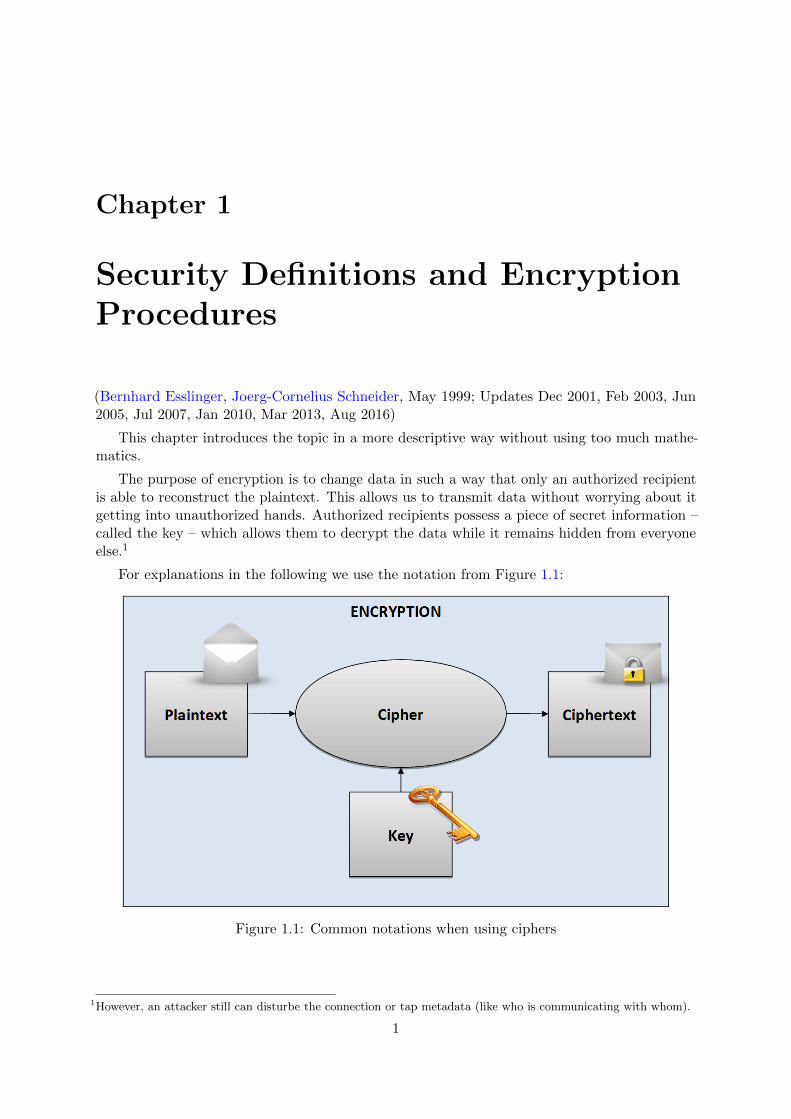
The purpose of encryption is to change data in such a way that only an authorized recipientis able to reconstruct the plaintext. This allows us to transmit data without worrying about itgetting into unauthorized hands. Authorized recipients possess a piece of secret information –called the key – which allows them to decrypt the data while it remains hidden from everyoneelse.1
For explanations in the following we use the notation from Figure 1.1:
Figure 1.1: Common notations when using ciphers
1However, an attacker still can disturbe the connection or tap metadata (like who is communicating with whom).
1

Explain it to me, I will forget it.Show it to me, maybe I will remember it.
Let me do it, and I will be good at it.
Quote 1: Saying from India
1.1 Security definitions and the importance of cryptology
First we present the ideas how the security of cryptosystems is defined.
Modern cryptography is heavily based on mathematical theory and computer science practice.Cryptographic algorithms are designed around computational hardness assumptions, makingsuch algorithms hard to break in practice by any adversary.
Depending on the adversary’s capabilities there are mainly two basic notations of securitydistinguished in literature (see e.g. Contemporary Cryptography [Opp11]):
• Computational, conditional or practical securityA cipher is computationally secure if it is theoretically possible to break such a systembut it is infeasible to do so by any known practical means. Theoretical advances (e.g.,improvements in integer factorization algorithms) and faster computing technology requirethese solutions to be continually adapted.
Even using the best known algorithm for breaking it will require so much resources (e.g.,1,000,000 years) that practically the cryptosystem is secure.
So this concept is based on assumptions of the adversary’s limited computing power andthe current state of science.
• Information-theoretical or unconditional securityA cipher is considered unconditionally secure if its security is guaranteed no matter howmuch resources (time, space) the attacker has – so even in the case where the adversaryhas unlimited resources for breaking a cipher. Even with unlimited resources an adversaryis unable to gain any meaningful data from a ciphertext.
There exist information-theoretically secure schemes that provably cannot be broken evenwith unlimited computing power – an example is the one-time pad (OTP).
As the OTP is information-theoretically secure it derives its security solely from informationtheory and is secure even with unlimited computing power at the adversary’s disposal.However, OTP has several practical disadvantages (the key used must be used only once,randomly selected and must be at least as long as the message being protected), whichmeans that it is hardly used except in closed environments such as for the hot wire betweenMoscow and Washington.
Two more concepts are sometimes used:
• Provable security This means that breaking such a cryptographic system is as difficultas solving some supposedly difficult problem e.g. discrete logarithm computation, discretesquare root computation, very large integer factorization.
Example: Currently we know that RSA is at most as difficult as factorization, but wecannot prove that its exactly as difficult as factorization. So RSA has no proven minimum
2

security. Or in other words: We cannot prove, that if RSA (the cryptosystem) is broken,that then factorization (the hard mathematical problem) can be solved.
The Rabin cryptosystem was the first cryptosystem which could be proven to be computa-tionally equivalent to a hard problem.
• Ad-hoc security A cryptographic system has this security feature if it is not worth totry to break into such a system because of inadequate price of data with comparison toprice of work needed to do so. Or an attack can’t be done in sufficiently short time (seeHandbook of Applied Cryptography [MvOV01]).
Example: This may apply if a message relevant for the stock market will be publishedtomorrow and you need a year to break it.
For good procedures used today the time taken to break them is so long that it is practicallyimpossible to do so, and these procedures can therefore be considered (practically) secure – froma pure algorithm’s point of view.2
We basically distinguish between symmetric (see chapter 1.3) and asymmetric (see chapter1.4) encryption procedures. The books of Bruce Schneier [Sch96b] and Klaus Schmeh [Sch16a]also offer a very good overview of the different encryption algorithms.3
With the use of the internet and wireless communication, encryption technologies areused (mostly transparently) by everyone. However, they have been in use since centuries bygovernments, military, and diplomats. The side which had a better command of these technologiescould exert big influence on politics and war with the help of secret services. This book onlytouches history when introducing the earlier cipher methods in chapter 2. You can gain animpression, how important cryptology was and still is, by considering the following two examples:the educational film “War of the letters” (German: Krieg der Buchstaben)4 and the debatesaround the so called crypto wars5.
2Especially after the knowledge gathered by Edward Snowden there were many discussions, whether encryption issecure. In [ESS14] is the result of an evaluation, which cryptographic algoritms can be relied on – according tocurrent knowledge. The article investigates: Which crypto systems can – despite the reveal of the NSA/GCHQattacks – still be considered as secure? Where have systems been intentionally weakened? How can we create asecure cryptographic future? Where is the difference between maths and implementation?
3A compact overview about what is used where, which methods are secure, where you have to anticipate problemsand where the construction areas will be in the future (incl. the lengthy procedures of the standardization) can befound in the German article [Sch16b].
4See http://bscw.schule.de/pub/bscw.cgi/d1269787/Krieg_der_Buchstaben.pdf.A supporting quote from Denis Smyth, professor in the Department of History and the International RelationsProgramme at the University of Toronto: “Secret intelligence has long been regarded as the “missing dimension”of international relations.” (from http://www.secretintelligencefiles.com)
5See https://en.wikipedia.org/wiki/Crypto_Wars.
3

“One cannot not communicate.”
Quote 2: Paul Watzlawick6
1.2 Influences on encryption methods
Here, we just want to mention two aspects often neglected and dealt with too late:
• Random basedAlgorithms can be divided up into deterministic and heuristic methods. Most students onlylearnt deterministic methods, where the output is uniquely determined by the input. Onthe other hand, heuristic methods make decisions using random values. Modern methodsof machine learning are also part of them.
Random looms large in cryptographic methods. Keys have to be selected randomly, whichmeans that at least for the key generation “random” is necessary. In addition, somemethods, especially from cryptanalysis, are heuristic.
• Constant basedMany modern methods (especially hash methods and symmetric encryption) use numericconstants. Their values should be plausible and they shouldn’t contain back doors. Numbersfulfilling this requirement are called nothing-up-my-sleeve numbers.7
6Paul Watzlawick, Janet H. Beavin, and Don D. Jackson, “Pragmatics of human communication; a study ofinteractional patterns, pathologies, and paradoxes”, Norton, 1967, The first of five axioms of their humancommunications theory.
7http://en.wikipedia.org/wiki/Nothing_up_my_sleeve_number
4
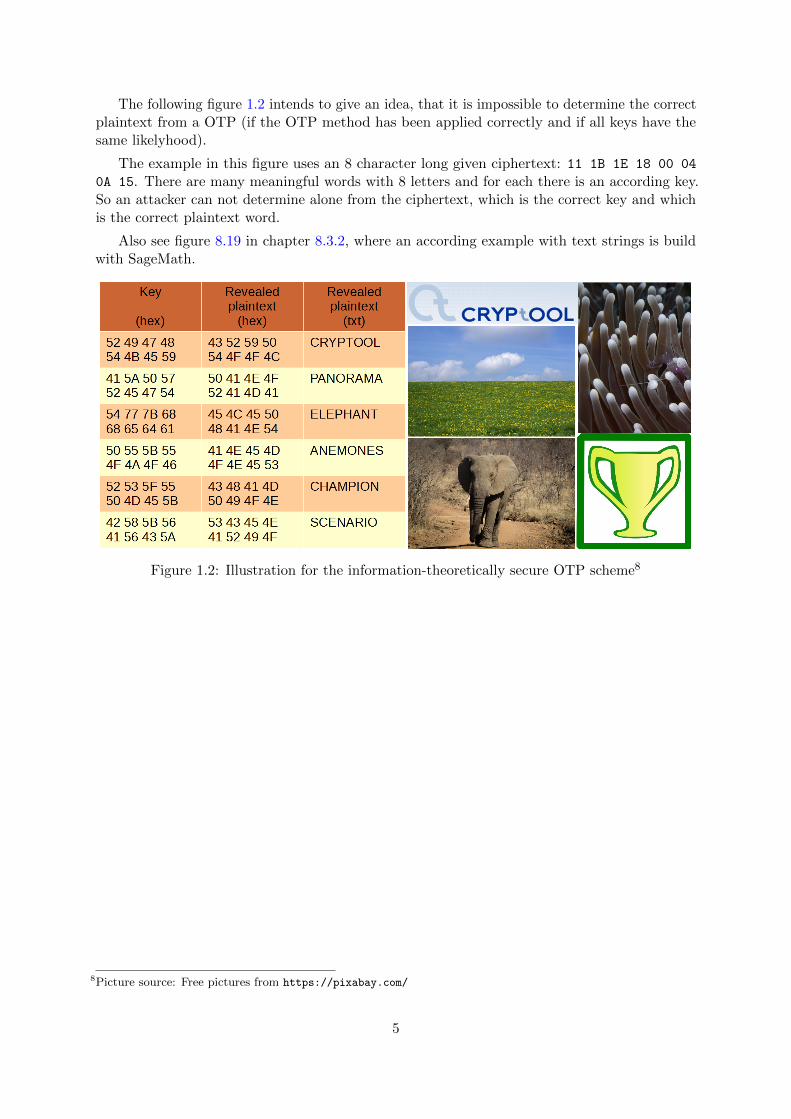
The following figure 1.2 intends to give an idea, that it is impossible to determine the correctplaintext from a OTP (if the OTP method has been applied correctly and if all keys have thesame likelyhood).
The example in this figure uses an 8 character long given ciphertext: 11 1B 1E 18 00 04
0A 15. There are many meaningful words with 8 letters and for each there is an according key.So an attacker can not determine alone from the ciphertext, which is the correct key and whichis the correct plaintext word.
Also see figure 8.19 in chapter 8.3.2, where an according example with text strings is buildwith SageMath.
Figure 1.2: Illustration for the information-theoretically secure OTP scheme8
8Picture source: Free pictures from https://pixabay.com/
5
“Transparency. That’s the best one can hope for in a technologically advanced society ...otherwise you will just be manipulated.”
Quote 3: Daniel Suarez9
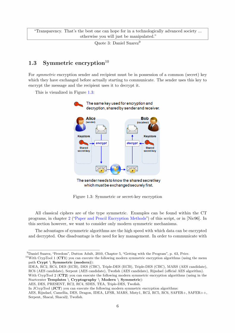
1.3 Symmetric encryption10
For symmetric encryption sender and recipient must be in possession of a common (secret) keywhich they have exchanged before actually starting to communicate. The sender uses this key toencrypt the message and the recipient uses it to decrypt it.
This is visualized in Figure 1.3:
Figure 1.3: Symmetric or secret-key encryption
All classical ciphers are of the type symmetric. Examples can be found within the CTprograms, in chapter 2 (“Paper and Pencil Encryption Methods”) of this script, or in [Nic96]. Inthis section however, we want to consider only modern symmetric mechanisms.
The advantages of symmetric algorithms are the high speed with which data can be encryptedand decrypted. One disadvantage is the need for key management. In order to communicate with
9Daniel Suarez, “Freedom”, Dutton Adult, 2010, Chapter 5, “Getting with the Program”, p. 63, Price.10With CrypTool 1 (CT1) you can execute the following modern symmetric encryption algorithms (using the menu
path Crypt \ Symmetric (modern)):IDEA, RC2, RC4, DES (ECB), DES (CBC), Triple-DES (ECB), Triple-DES (CBC), MARS (AES candidate),RC6 (AES candidate), Serpent (AES candidate), Twofish (AES candidate), Rijndael (official AES algorithm).With CrypTool 2 (CT2) you can execute the following modern symmetric encryption algorithms (using in theStartcenter Templates \ Cryptography \ Modern \ Symmetric):AES, DES, PRESENT, RC2, RC4, SDES, TEA, Triple-DES, Twofish.In JCrypTool (JCT) you can execute the following modern symmetric encryption algorithms:AES, Rijndael, Camellia, DES, Dragon, IDEA, LFSR, MARS, Misty1, RC2, RC5, RC6, SAFER+, SAFER++,Serpent, Shacal, Shacal2, Twofish.
6

one another confidentially, sender and recipient must have exchanged a key using a secure channelbefore actually starting to communicate. Spontaneous communication between individuals whohave never met therefore seems virtually impossible. If everyone wants to communicate witheveryone else spontaneously at any time in a network of n subscribers, each subscriber musthave previously exchanged a key with each of the other n− 1 subscribers. A total of n(n− 1)/2keys must therefore be exchanged.
1.3.1 AES (Advanced Encryption Standard)11
Before AES, the most well-known modern symmetric encryption procedure was the DES algorithm.The DES algorithm has been developed by IBM in collaboration with the National SecurityAgency (NSA), and was published as a standard in 1975. Despite the fact that the procedure isrelatively old, no effective attack on it has yet been detected. The most effective way of attackingconsists of testing (almost) all possible keys until the right one is found (brute-force-attack). Dueto the relatively short key length of effectively 56 bits (64 bits, which however include 8 paritybits), numerous messages encrypted using DES have in the past been broken. Therefore, theprocedure can not be considered secure any longer. Alternatives to the DES procedure includeIDEA, Triple-DES (TDES) and especially AES.
Up-to-the-minute procedure for symmetric ciphers is the AES. The associated Rijndaelalgorithm was declared winner of the AES award on October 2nd, 2000 and thus succeeds theDES procedure.
An introduction and further references about the AES algorithms and the AES candidatesof the last round can be found i.e. within the online help of CrypTool12 oder in Wikipedia13.
11In CT1 you can find 3 visualizations for this cipher via the menu Indiv. Procedures \ Visualization ofAlgorithms \ AES.In CT2 you can find a template performing AES step-by-step (by entering the search string “AES” in theStartcenter).
12CrypTool 1 online help: The index head-word AES leads to the 3 help pages: AES candidates, The AESwinner Rijndael and The Rijndael encryption algorithmA comprehensive description of AES including C code can be found in [Haa08].
13https://en.wikipedia.org/wiki/Advanced_Encryption_Standard
7
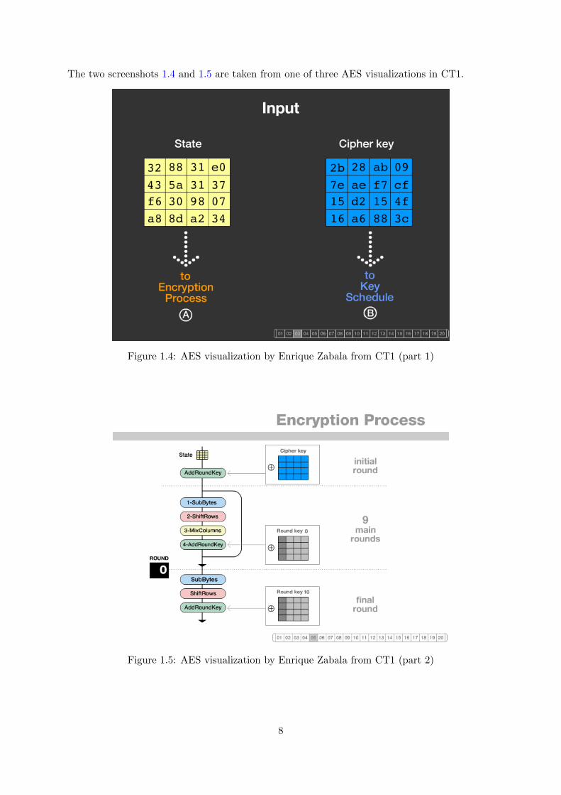
The two screenshots 1.4 and 1.5 are taken from one of three AES visualizations in CT1.
Figure 1.4: AES visualization by Enrique Zabala from CT1 (part 1)
Figure 1.5: AES visualization by Enrique Zabala from CT1 (part 2)
8

Now we want to encrypt with AES in CBC mode a 128-bit block of plaintext. Off the resultingciphertext we are only interested in the 1st block (if there is more, it would be padding, herenull-padding). For demonstration we do it once with CT2 and once with OpenSSL.
Figure 1.6 shows the encryption of one block in CT2.
The plaintext “AESTEST1USINGCT2” is converted to hex (41 45 53 54 45 53 54 31 55 5349 4E 47 43 54 32). Using this and the key 3243F6A8885A308D313198A2E0370734 the AEScomponent creates the ciphertext. It is in hex:B1 13 D6 47 DB 75 C6 D8 47 FD 8B 92 9A 29 DE 08
Figure 1.6: AES encryption (of exactly 1 block and without padding) in CT2
The same result can be achieved with OpenSSL14 from the commandline:
OpenSSL sample 1.1 AES encryption (of exactly one block and without padding) in OpenSSL>openssl enc -e -aes-128-cbc
-K 3243F6A8885A308D313198A2E0370734
-iv 00000000000000000000000000000000
-in klartext-1.hex -out klartext-1.hex.enc
>dir
06.07.2016 12:43 16 key.hex
20.07.2016 20:19 16 klartext-1.hex
20.07.2016 20:37 32 klartext-1.hex.enc
14OpenSSL is a very widespread free open-source crypto library, used by many applications, for instance to implementthe TLS protocol. Part of OpenSSL is the commandline tool openssl, which can be used to test the functionalitydirectly on many operating systems and to request, create and manage certificates.Contrarily to the also very widespread and very good commandline tool gpg from GNU Privacy Guard (https://en.wikipedia.org/wiki/GNU_Privacy_Guard), openssl also allows calls with many details. The gpg has itsfocus on the practically applied ciphersuites. As far as we know, it is not possible to encrypt just one blockwithout padding with the commandline tool gpg.Also see https://en.wikipedia.org/wiki/OpenSSL.
9

1.3.1.1 Results about theoretical cryptanalysis of AES
Below you will find some results, which have recently called into question the security of theAES algorithm – from our point of view these doubts practically still remain unfounded . Thefollowing information is based particularly on the original papers and the articles [Wob02] and[LW02].
AES with a minimum key length of 128 bit is still in the long run sufficiently secure againstbrute-force attacks – as long as the quantum computers aren’t powerful enough. When announcedas new standard AES was immune against all known cryptanalytic attacks, mostly based onstatistical considerations and earlier applied to DES: using pairs of clear and cipher textsexpressions are constructed, which are not completely at random, so they allow conclusions tothe used keys. These attacks required unrealistically large amounts of intercepted data.
Cryptanalysts already label methods as “academic success” or as “cryptanalytic attack” ifthey are theoretically faster than the complete testing of all keys (brute force analysis). In thecase of AES with the maximal key length (256 bit) exhaustive key search on average needs 2255
encryption operations. A cryptanalytic attack needs to be better than this. At present between275 and 290 encryption operations are estimated to be performable only just for organizations,for example a security agency.
In their 2001-paper Ferguson, Schroeppel and Whiting [FSW01] presented a new method ofsymmetric codes cryptanalysis: They described AES with a closed formula (in the form of acontinued fraction) which was possible because of the “relatively” clear structure of AES. Thisformula consists of around 1000 trillion terms of a sum - so it does not help concrete practicalcryptanalysis. Nevertheless curiosity in the academic community was awakened. It was alreadyknown, that the 128-bit AES could be described as an over-determined system of about 8000quadratic equations (over an algebraic number field) with about 1600 variables (some of themare the bits of the wanted key) – equation systems of that size are in practice not solvable. Thisspecial equation system is relatively sparse, so only very few of the quadratic terms (there areabout 1,280,000 are possible quadratic terms in total) appear in the equation system.
The mathematicians Courtois and Pieprzyk [CP02] published a paper in 2002, which gota great deal of attention amongst the cryptology community: The pair had further developedthe XL-method (eXtended Linearization), introduced at Eurocrypt 2000 by Shamir et al., tocreate the so called XSL-method (eXtended Sparse Linearization). The XL-method is a heuristictechnique, which in some cases manages to solve big non-linear equation systems and whichwas till then used to analyze an asymmetric algorithm (HFE). The innovation of Courtois andPieprzyk was, to apply the XL-method on symmetric codes: the XSL-method can be applied tovery specific equation systems. A 256-bit AES could be attacked in roughly 2230 steps. This isstill a purely academic attack, but also a direction pointer for a complete class of block ciphers.The major problem with this attack is that until now nobody has worked out, under whatconditions it is successful: the authors specify in their paper necessary conditions, but it is notknown, which conditions are sufficient. There are two very new aspects of this attack: firstlythis attack is not based on statistics but on algebra. So attacks seem to be possible, where onlyvery small amounts of ciphertext are available. Secondly the security of a product algorithm15
15A ciphertext can be used as input for another encryption algorithm. A cascade cipheris build up as a compositionof different encryption transformations. The overall cipher is called product algorithm or cascade cipher (sometimesdepending whether the used keys are statistically dependent or not).Cascading does not always improve the security.This process is also used within modern algorithms: They usually combine simple and, considered at its own,cryptologically relatively insecure single steps in several rounds into an efficient overall procedure. Most blockciphers (e.g. DES, IDEA) are cascade ciphers.
10

does not exponentially increase with the number of rounds.
Currently there is a large amount of research in this area: for example Murphy and Robshawpresented a paper at Crypto 2002 [MR02b], which could dramatically improve cryptanalysis: theburden for a 128-bit key was estimated at about 2100 steps by describing AES as a special caseof an algorithm called BES (Big Encryption System), which has an especially “round” structure.But even 2100 steps are beyond what is achievable in the foreseeable future. Using a 256 bit keythe authors estimate that a XSL-attack will require 2200 operations.
More details can be found in the Web links section at “AES or Rijndael cryptosystem”.
So for AES-256 the attack is much more effective than brute-force but still far away fromany computing power which could be accessible in the short-to-long term.
The discussion temporarily was very controversial: Don Coppersmith (one of the inventors ofDES) for example queries the practicability of the attack because XLS would provide no solutionfor AES [Cop02]. This implies that then the optimization of Murphy and Robshaw [MR02a]would not work.
In 2009 Biryukov and Khovratovich [BK09] published another theoretical attack on AES.This attack uses different methods from the ones described above. They applied methods fromhash function cryptanalysis (local collisions and boomerang switching) to construct a related-keyattack on AES-256. I. e. the attacker not only needs to be able to encrypt arbitrary data (chosenplain text), in addition he needs to be able to manipulate the unknown key (related-key).
Based on those assumptions, the effort to find a AES-256 key is reduced to 2119 time and 277
memory (considering asymmetric complexity). In the case of AES-192 the attack is even lesspractical, for AES-128 the authors do not provide an attack.
1.3.2 Algebraic or algorithmic cryptanalysis on symmetric algorithms
There are different modern methods attacking the structure of a problem directly or after atransformation of the problem. One of the attack methods is based on the satisfiability problem(SAT)16.
Description of a SAT solver
An old and well-studied problem in computer science is called the SAT problem. Here, for agiven Boolean formula, it’s the task to find out whether there is an assignment of the variables,so that the evaluation result of the formula is 1.
Example: The Boolean formula “A AND B” evaluates to 1, if and only if A=B=1. For theformula “A AND NOT(A)” there exists no assignment of its variable A, so that the formula isevaluated to the value 1.
For larger Boolean formulas, it is not easy to determine if an assignment exists for which theformula can be evaluated to 1 (this problem belongs to the NP-complete problems). Thereforespecific tools have been developed to solve this problem for general Boolean formulas, so calledSAT solvers17. As has been found, SAT solvers can also be used to attack cryptographic systems.
SAT solver based cryptanalysis
Also serial usage of the same cipher with different keys (like with Triple-DES) is called cascade cipher.16http://en.wikipedia.org/wiki/Boolean_satisfiability_problem17With CT2 you can execute a SAT solver – using in the Startcenter Templates \ Mathematics \ SAT Solver
(Text Input) and SAT Solver (File Input).
11
The general approach to use SAT solvers in cryptanalysis is very straightforward: First, thecryptographic problem, e.g. finding the symmetric key or an inversion of a hash function, istranslated into a SAT problem. Then, the SAT solver can be used to find a solution to the SATproblem. The solution of the SAT problem then also solves the original cryptographic problem.The paper by Massacci [MM00] describes the first known usage of a SAT solver in this context.Unfortunately, very soon it turned out that such a general approach cannot be used efficientlyin practice. This is due to the fact that the cryptographic SAT problems are very complex andthe runtime of a SAT solver increases exponentially with the problem size. Therefore, in modernapproaches SAT solvers are used only for solving partial problems of cryptanalysis. A goodexample for this is described in the paper by Mironov and Zhang [MZ06]. They demonstratethe usage of a SAT solver in an attack on hash functions, where the SAT solver is used to solvesome partial problems in a very efficient way.
1.3.3 Current status of brute-force attacks on symmetric algorithms
The current status of brute-force attacks on symmetric encryption algorithms can be explainedwith the block cipher RC5.
Brute-force (exhaustive search, trial-and-error) means to completely examine all keys of thekey space: so no special analysis methods have to be used. Instead, the ciphertext is decryptedwith all possible keys18 and for each resulting text it is checked, whether this is a meaningfulclear text19. A key length of 64 bit means at most 264 = 18,446,744,073,709,551,616 or about 18trillion (GB) / 18 quintillion (US) keys to check.
Companies like RSA Security provided so-called cipher challenges in order to quantify thesecurity offered by well-known symmetric ciphers as DES, Triple-DES or RC5.20 They offeredprizes for those who managed to decipher ciphertexts, encrypted with different algorithmsand different key lengths, and to unveil the symmetric key (under controlled conditions). Sotheoretical estimates can be confirmed.
It is well-known, that the “old” standard algorithm DES with a fixed key length of 56 bitis no more secure: This was demonstrated already in January 1999 by the Electronic FrontierFoundation (EFF). With their specialized computer Deep Crack they cracked a DES encryptedmessage within less than a day.21
The current record for strong symmetric algorithms unveiled a key 64 bit long. The algorithmused was RC5, a block cipher with variable key size.
18With CT1 you can also perform brute-force attacks of modern symmetric algorithms (using the menu pathAnalysis \ Symmetric Encryption (modern)): Here the weakest knowledge of an attacker is assumed, heperforms a ciphertext-only attack.With CT2 you can also perform brute-force attacks (using the templates under Cryptanalysis \ Modern).Highly powerful is the KeySearcher component, which can be used to distribute the calculations to many differentcomputers.
19If the cleartext is written in a natural language and at least 100 B long, this check also can be performedautomatically.To achieve a result in an appropriate time with a single PC you should mark not more than 24 bit of the key asunknown.
20https://www.emc.com/emc-plus/rsa-labs/historical/the-rsa-laboratories-secret-key-challenge.htm
Unfortunately, in May 2007 RSA Inc announced that they will not confirm the correctness of the not yet solvedRC5-72 challenge.
There are also cipher challenges for asymmetric algorithms (please see chapter 4.11.4).A wide spectrum of both simple and complex, both symmetric and asymmetric crypto riddles are included in
the international cipher contest MysteryTwister C3: http://www.mysterytwisterc3.org.21https://www.emc.com/emc-plus/rsa-labs/historical/des-challenge-iii.htm
12

The RC5-64 challenge has been solved in July 2002 by the distributed.net team after 5years.22 In total 331,252 individuals co-operated over the internet to find the key.23 More than15 trillion (GB) / 15 quintillion (US) keys were checked, until they found the right key.24
So, symmetric algorithms (even if they have no cryptographic weakness) using keys of size64 bit are no more appropriate to keep sensible data private.
22http://www.distributed.net/Pressroom_press-rc5-64
http://www.distributed.net/images/9/92/20020925_-_PR_-_64_bit_solved.pdf23An overview of current distributed computing projects can be found here:http://distributedcomputing.info/
24CT2 started to experiment with a general infrastructure for distributed computing called CrypCloud (bothpeer-to-peer and centralized). So in the future, CT2 will be able to distribute the calculations on many computers.What could be achieved after the components are made ready for parallelization showed a cluster for distributedcryptanalysis of DES and AES: Status on March 21st, 2016 is, that an AES brute-force attack (distributedkeysearching) worked on 50 i5 PCs, each with 4 virtual CPU cores. These 200 virtual “worker threads” achievedto test about 350 million AES keys/sec. The “cloud” processed a total amount of about 20 GB/sec of data.CrypCloud is a volunteering cloud system which enables CT2 users to voluntarily join distributed computing jobs.
13
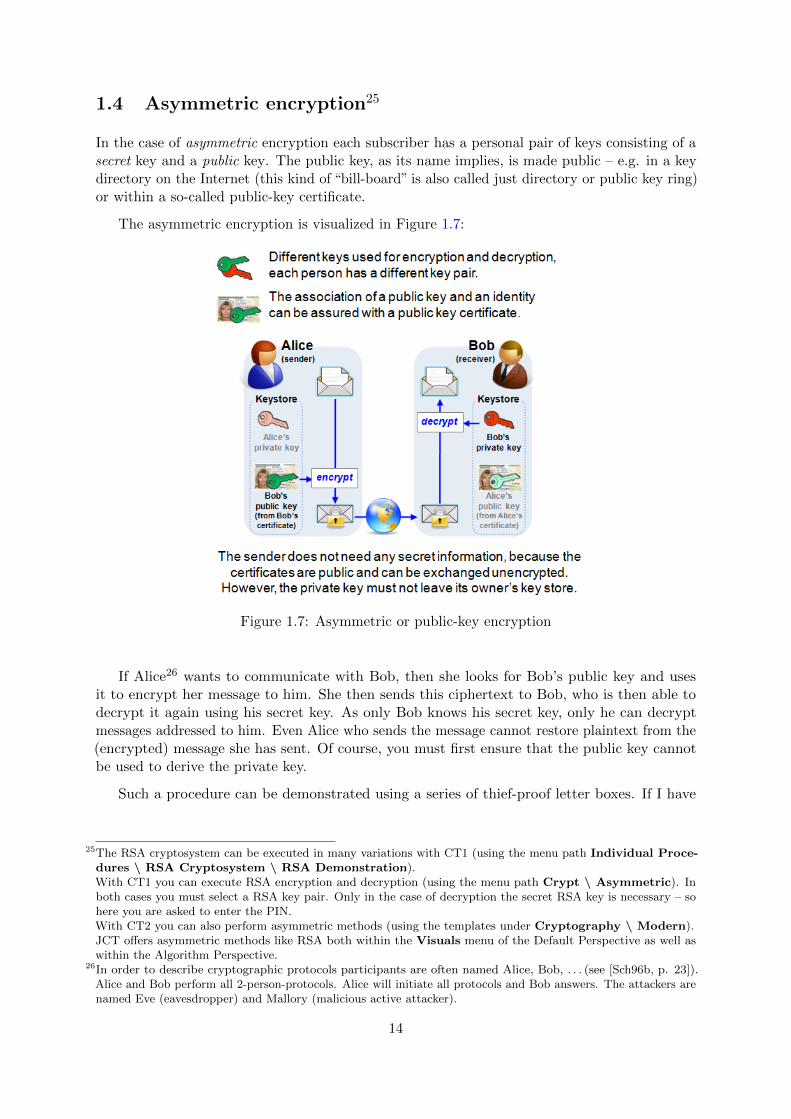
1.4 Asymmetric encryption25
In the case of asymmetric encryption each subscriber has a personal pair of keys consisting of asecret key and a public key. The public key, as its name implies, is made public – e.g. in a keydirectory on the Internet (this kind of “bill-board” is also called just directory or public key ring)or within a so-called public-key certificate.
The asymmetric encryption is visualized in Figure 1.7:
Figure 1.7: Asymmetric or public-key encryption
If Alice26 wants to communicate with Bob, then she looks for Bob’s public key and usesit to encrypt her message to him. She then sends this ciphertext to Bob, who is then able todecrypt it again using his secret key. As only Bob knows his secret key, only he can decryptmessages addressed to him. Even Alice who sends the message cannot restore plaintext from the(encrypted) message she has sent. Of course, you must first ensure that the public key cannotbe used to derive the private key.
Such a procedure can be demonstrated using a series of thief-proof letter boxes. If I have
25The RSA cryptosystem can be executed in many variations with CT1 (using the menu path Individual Proce-dures \ RSA Cryptosystem \ RSA Demonstration).With CT1 you can execute RSA encryption and decryption (using the menu path Crypt \ Asymmetric). Inboth cases you must select a RSA key pair. Only in the case of decryption the secret RSA key is necessary – sohere you are asked to enter the PIN.With CT2 you can also perform asymmetric methods (using the templates under Cryptography \ Modern).JCT offers asymmetric methods like RSA both within the Visuals menu of the Default Perspective as well aswithin the Algorithm Perspective.
26In order to describe cryptographic protocols participants are often named Alice, Bob, . . . (see [Sch96b, p. 23]).Alice and Bob perform all 2-person-protocols. Alice will initiate all protocols and Bob answers. The attackers arenamed Eve (eavesdropper) and Mallory (malicious active attacker).
14

composed a message, I then look for the letter box of the recipient and post the letter throughit. After that, I can no longer read or change the message myself, because only the legitimaterecipient has the key for the letter box.
The advantage of asymmetric procedures is the easier key management. Let’s look again at anetwork with n subscribers. In order to ensure that each subscriber can establish an encryptedconnection to each other subscriber, each subscriber must possess a pair of keys. We thereforeneed 2n keys or n pairs of keys. Furthermore, no secure channel is needed before messages aretransmitted, because all the information required in order to communicate confidentially canbe sent openly. In this case, you simply27 have to pay attention to the accuracy (integrity andauthenticity) of the public key. Disadvantage: Pure asymmetric procedures take a lot longer toperform than symmetric ones.
The most well-known asymmetric procedure is the RSA algorithm28, named after its devel-opers Ronald Rivest, Adi Shamir and Leonard Adleman. The RSA algorithm was publishedin 1978.29 The concept of asymmetric encryption was first introduced by Whitfield Diffie andMartin Hellman in 1976. Today, the ElGamal procedures also play a decisive role, particularlythe Schnorr variant in the DSA (Digital Signature Algorithm).
Attacks against asymmetric ciphers are touched in- chapter 4: Elementary Number Theory,- chapter 5: Modern Cryptography,- chapter 7: Elliptic Curves, and- chapter 10: Current Results for Solving Discrete Logarithms And Factoring.
27That this is also not trivial is explained e.g. in chapter 4.11.5.4. Besides the requirements for the key generationit has to be considered that nowadays also (public-key) infrastructures itself are targets of cyber attacks.
28The RSA algorithm is extensively described in chapter 4.10 and later within this script. The topical researchresults concerning RSA are described in chapter 4.11.
29Hints about the history of RSA and its publication which didn’t amuse the NSA can be found within the seriesRSA & Co. at school: Modern cryptology, old mathematics, and subtle protocols. Unfortunately these are currentlyonly available in German. See [WS06], pp 55 ff (“Penible Lammergeier”).
15

1.5 Hybrid procedures30
In order to benefit from the advantages of symmetric and asymmetric techniques together, hybridprocedures are usually used (for encryption) in practice.
In this case the bulk data is encrypted using symmetric procedures: The key used for this isa secret session key generated by the sender randomly31 that is only used for this message.
This session key is then encrypted using the asymmetric procedure, and transmitted to therecipient together with the message.
Recipients can determine the session key using their private keys and then use the sessionkey to encrypt the message.
In this way, we can benefit from the easy key management of asymmetric procedures (usingpublic/private keys) and we benefit from the efficiency of symmetric procedures to encrypt largequantities of data (using secret keys).
30Within CT1 you can find this technique using the menu path Crypt \ Hybrid: There you can follow thesingle steps and its dependencies with concrete numbers. The variant with RSA as the asymmetric algorithmis graphically visualized; the variant with ECC uses the standard dialogs. In both cases AES is used as thesymmetric algorithm.JCT offers hybrid methods like ECIES within the Algorithm Perspective under Algorithms \ Hybrid Ciphers.
31An important part of cryptographically secure techniques is to generate random numbers.- Within CT1 you can check out different random number generators (PRNGs) using the menu path Indiv.Procedures \ Generate Random Numbers. Using the menu path Analysis \ Analyze Randomness youcan apply different test methods for random data to binary documents.- In CT2 you can find templates using PRNGs (by entering the search string “random” in the Startcenter). ThePRNGs internally use for instance Keccak or the Linear Congruential Generator (LCG), and they are used e.g.for key generation or decimalization.- JCT offers pseudo random number generators both within the Default Perspective in the menu Algorithms \Random Number Generator as well as within the Algorithm Perspective.
16
There is an old saying inside the US National Security Agency (NSA):“Attacks always get better; they never get worse.”
Quote 4: IETF32
1.6 Cryptanalysis and symmetric ciphers for educational pur-poses33
Compared to public-key ciphers based on mathematics like RSA, the structure of AES and mostother modern symmetric ciphers (like DES, IDEA or Present), is very complex and cannot beexplained as easily as RSA.
So simplified variants of modern symmetric ciphers were developed for educational purposesin order to allow beginners to perform encryption and decryption by hand and gain a betterunderstanding of how the algorithms work in detail. These simplified variants also help tounderstand and apply the according cryptanalysis methods.
The most well-known of these variants are SDES (Simplified DES)34 and S-AES (Simplified-AES) by Prof. Ed Schaefer and his students35, and Mini-AES (see chapter 1.8.1 “Mini-AES”):
• Edward F. Schaefer: A Simplified Data Encryption Standard Algorithm [Sch96a].
• Raphael Chung-Wei Phan: Mini Advanced Encryption Standard (Mini-AES): A Testbedfor Cryptanalysis Students [Pha02].
• Raphael Chung-Wei Phan: Impossible differential cryptanalysis of Mini-AES [Pha03].
• Mohammad A. Musa, Edward F. Schaefer, Stephen Wedig: A simplified AES algorithmand its linear and differential cryptanalyses [MSW03].
• Nick Hoffman: A SIMPLIFIED IDEA ALGORITHM [Hof06].
• S. Davod. Mansoori, H. Khaleghei Bizaki: On the vulnerability of Simplified AES AlgorithmAgainst Linear Cryptanalysis [MB07].
1.7 Further information
Beside the information you can find in the following chapters, in many other books and on agood number of websites, the online help of all CrypTool variants also offer very many detailsabout the symmetric and asymmetric encryption methods.
32http://tools.ietf.org/html/rfc427033A very good starting point to learn cryptanalysis is the book from Mark Stamp [SL07]. Also good, but very
high-level and concentrating on analyzing symmetric block ciphers only, is the article from Bruce Schneier [Sch00].Several of the cipher challenges at “MysteryTwister C3” (http://www.mysterytwisterc3.org) are also wellsuitable for educational purposes.
34If you double-click on the title of the icon of the SDES component in CT2 you can see a visualiza-tion of the SDES algorithm, showing how the bits of the given data flow through the whole algorithm.An according screenshot: https://www.facebook.com/CrypTool2/photos/a.505204806238612.1073741827.
243959195696509/59735442369031635See the article “Devising a Better Way to Teach and Learn the Advanced Encryption Standard” at http:
//math.scu.edu/~eschaefe/getfile.pdf
17
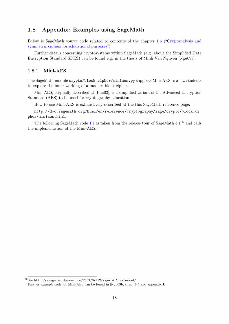
1.8 Appendix: Examples using SageMath
Below is SageMath source code related to contents of the chapter 1.6 (“Cryptanalysis andsymmetric ciphers for educational purposes”).
Further details concerning cryptosystems within SageMath (e.g. about the Simplified DataEncryption Standard SDES) can be found e.g. in the thesis of Minh Van Nguyen [Ngu09a].
1.8.1 Mini-AES
The SageMath module crypto/block_cipher/miniaes.py supports Mini-AES to allow studentsto explore the inner working of a modern block cipher.
Mini-AES, originally described at [Pha02], is a simplified variant of the Advanced EncryptionStandard (AES) to be used for cryptography education.
How to use Mini-AES is exhaustively described at the this SageMath reference page:
http://doc.sagemath.org/html/en/reference/cryptography/sage/crypto/block_ci
pher/miniaes.html.
The following SageMath code 1.1 is taken from the release tour of SageMath 4.136 and callsthe implementation of the Mini-AES.
36See http://mvngu.wordpress.com/2009/07/12/sage-4-1-released/.Further example code for Mini-AES can be found in [Ngu09b, chap. 6.5 and appendix D].
18

SageMath sample 1.1 Encryption and decryption with Mini-AES# We can encrypt a plaintext using Mini-AES as follows:
sage: from sage.crypto.block_cipher.miniaes import MiniAES
sage: maes = MiniAES()
sage: K = FiniteField(16, "x")
sage: MS = MatrixSpace(K, 2, 2)
sage: P = MS([K("x^3 + x"), K("x^2 + 1"), K("x^2 + x"), K("x^3 + x^2")]); P
[ x^3 + x x^2 + 1]
[ x^2 + x x^3 + x^2]
sage: key = MS([K("x^3 + x^2"), K("x^3 + x"), K("x^3 + x^2 + x"), K("x^2 + x + 1")]); key
[ x^3 + x^2 x^3 + x]
[x^3 + x^2 + x x^2 + x + 1]
sage: C = maes.encrypt(P, key); C
[ x x^2 + x]
[x^3 + x^2 + x x^3 + x]
# Here is the decryption process:
sage: plaintxt = maes.decrypt(C, key)
sage: plaintxt == P
True
# We can also work directly with binary strings:
sage: from sage.crypto.block_cipher.miniaes import MiniAES
sage: maes = MiniAES()
sage: bin = BinaryStrings()
sage: key = bin.encoding("KE"); key
0100101101000101
sage: P = bin.encoding("Encrypt this secret message!")
sage: C = maes(P, key, algorithm="encrypt")
sage: plaintxt = maes(C, key, algorithm="decrypt")
sage: plaintxt == P
True
# Or work with integers n such that 0 <= n <= 15:
sage: from sage.crypto.block_cipher.miniaes import MiniAES
sage: maes = MiniAES()
sage: P = [n for n in xrange(16)]; P
[0, 1, 2, 3, 4, 5, 6, 7, 8, 9, 10, 11, 12, 13, 14, 15]
sage: key = [2, 3, 11, 0]; key
[2, 3, 11, 0]
sage: P = maes.integer_to_binary(P)
sage: key = maes.integer_to_binary(key)
sage: C = maes(P, key, algorithm="encrypt")
sage: plaintxt = maes(C, key, algorithm="decrypt")
sage: plaintxt == P
True
19

1.8.2 Further symmetric crypto algorithms in SageMath
The Reference for SageMath v7.2 lists e.g. the following further cryptographic functions:37
• Linear feedback shift register (LFSR),
• Blum-Blum-Shub (BBS): pseudo-random generator (to be found with streams),
• Lattice-based functions.
37See http://doc.sagemath.org/html/en/reference/sage/crypto/index.html,http://doc.sagemath.org/html/en/reference/cryptography/index.html, andhttp://combinat.sagemath.org/doc/reference/cryptography/sage/crypto/stream.html
20

Bibliography (Chap CryptoMeth)
[BK09] Biryukov, Alex and Dmitry Khovratovich: Related-key Cryptanalysis of the FullAES-192 and AES-256. Cryptology ePrint Archive, 2009. http://eprint.iacr.org/2009/317.
[Cop02] Coppersmith, Don: Re: Impact of Courtois and Pieprzyk results. Journal unknown,2002.http://csrc.nist.gov/archive/aes/ Former link from the AES DiscussionGroups.
[CP02] Courtois, Nicolas and Josef Pieprzyk: Cryptanalysis of Block Ciphers with OverdefinedSystems of Equations. Cryptology ePrint Archive, 2002.A different, so called compact version of the first XSL attack, was published in theproceedings for Asiacrypt Dec 2002. http://eprint.iacr.org/2002/044.
[ESS14] Esslinger, B., J. Schneider, and V. Simon: Krypto + NSA = ? – Kryptografi-sche Folgerungen aus der NSA-Affare. KES Zeitschrift fur Informationssicherheit,2014(1):70–77, March 2014.https://www.cryptool.org/images/ctp/documents/krypto_nsa.pdf.
[FSW01] Ferguson, Niels, Richard Schroeppel, and Doug Whiting: A simple algebraic repre-sentation of Rijndael, 2001.http://citeseerx.ist.psu.edu/viewdoc/summary?doi=10.1.1.28.4921.
[Haa08] Haan, Kristian Laurent: Advanced Encryption Standard (AES), 2008. http://www.codeplanet.eu/tutorials/cpp/51-advanced-encryption-standard.html.
[Hof06] Hoffman, Nick: A SIMPLIFIED IDEA ALGORITHM, 2006. http://www.nku.edu/~christensen/simplified%20IDEA%20algorithm.pdf.
[LW02] Lucks, Stefan and Rudiger Weis: Neue Ergebnisse zur Sicherheit des Verschlusse-lungsstandards AES. DuD, December 2002.
[MB07] Mansoori, S. Davod and H. Khaleghei Bizaki: On the vulnerability of Simplified AESAlgorithm Against Linear Cryptanalysis. IJCSNS International Journal of ComputerScience and Network Security, 7(7):257–263, 2007.http://paper.ijcsns.org/07_book/200707/20070735.pdf.
[MM00] Massacci, Fabio and Laura Marraro: Logical Cryptanalysis as a SAT Problem: En-coding and Analysis. Journal of Automated Reasoning Security, 24:165–203, 2000.
[MR02a] Murphy, S. P. and M. J. B. Robshaw: Comments on the Security of the AES and theXSL Technique, September 2002. http://crypto.rd.francetelecom.com/people/Robshaw/rijndael/rijndael.html.
21

[MR02b] Murphy, S. P. and M. J. B. Robshaw: Essential Algebraic Structure within the AES.Technical report, Crypto 2002, 2002. http://crypto.rd.francetelecom.com/pe
ople/Robshaw/rijndael/rijndael.html.
[MSW03] Musa, Mohammad A., Edward F. Schaefer, and Stephen Wedig: A simplified AESalgorithm and its linear and differential cryptanalyses. Cryptologia, 17(2):148–177,April 2003.http://www.rose-hulman.edu/~holden/Preprints/s-aes.pdf,http://math.scu.edu/eschaefe/ Ed Schaefer’s homepage.
[MvOV01] Menezes, Alfred J., Paul C. van Oorschot, and Scott A. Vanstone: Handbook ofApplied Cryptography. Series on Discrete Mathematics and Its Application. CRCPress, 5th edition, 2001, ISBN 0-8493-8523-7. (Errata last update Jan 22, 2014).http://cacr.uwaterloo.ca/hac/,http://www.cacr.math.uwaterloo.ca/hac/.
[MZ06] Mironov, Ilya and Lintao Zhang: Applications of SAT Solvers to Cryptanalysis ofHash Functions. Springer, 2006.
[Ngu09a] Nguyen, Minh Van: Exploring Cryptography Using the Sage Computer Algebra System.Master’s thesis, Victoria University, 2009.http://www.sagemath.org/files/thesis/nguyen-thesis-2009.pdf,http://www.sagemath.org/library-publications.html.
[Ngu09b] Nguyen, Minh Van: Number Theory and the RSA Public Key Cryptosystem – Anintroductory tutorial on using SageMath to study elementary number theory andpublic key cryptography, 2009. http://faculty.washington.edu/moishe/hanoie
x/Number%20Theory%20Applications/numtheory-crypto.pdf.
[Nic96] Nichols, Randall K.: Classical Cryptography Course, Volume 1 and 2. Technicalreport, Aegean Park Press 1996, 1996. 12 lessons.www.apprendre-en-ligne.net/crypto/bibliotheque/lanaki/lesson1.htm.
[Opp11] Oppliger, Rolf: Contemporary Cryptography, Second Edition. Artech House, 2nd edi-tion, 2011. http://books.esecurity.ch/cryptography2e.html.
[Pha02] Phan, Raphael Chung Wei: Mini Advanced Encryption Standard (Mini-AES): ATestbed for Cryptanalysis Students. Cryptologia, 26(4):283–306, 2002.
[Pha03] Phan, Raphael Chung Wei: Impossible differential cryptanalysis of Mini-AES. Cryp-tologia, 2003.http://www.tandfonline.com/doi/abs/10.1080/0161-110391891964.
[Sch96a] Schaefer, Edward F.: A Simplified Data Encryption Standard Algorithm. Cryptologia,20(1):77–84, 1996.
[Sch96b] Schneier, Bruce: Applied Cryptography, Protocols, Algorithms, and Source Code in C.Wiley, 2nd edition, 1996.
[Sch00] Schneier, Bruce: A Self-Study Course in Block-Cipher Cryptanalysis. Cryptologia,24:18–34, 2000. www.schneier.com/paper-self-study.pdf.
22

[Sch16a] Schmeh, Klaus: Kryptographie – Verfahren, Protokolle, Infrastrukturen.dpunkt.verlag, 6th edition, 2016. Sehr gut lesbares, aktuelles und umfang-reiches Buch uber Kryptographie. Geht auch auf praktische Probleme (wieStandardisierung oder real existierende Software) ein.
[Sch16b] Schmidt, Jurgen: Kryptographie in der IT – Empfehlungen zu Verschlusselung undVerfahren. c’t, 2016(1), 2016.Dieser Artikel erschien ursprunglich in c’t 01/2016, Seite 174. Danach veroffentlichtam 17.06.2016 in:http://www.heise.de/security/artikel/Kryptographie-in-der-IT-
Empfehlungen-zu-Verschluesselung-und-Verfahren-3221002.html.
[SL07] Stamp, Mark and Richard M. Low: Applied Cryptanalysis: Breaking Ciphers in theReal World. Wiley-IEEE Press, 2007.http://cs.sjsu.edu/faculty/stamp/crypto/.
[Wob02] Wobst, Reinhard: Angekratzt – Kryptoanalyse von AES schreitet voran. iX, December2002. (Und der Leserbrief dazu von Johannes Merkle in der iX 2/2003).
[WS06] Witten, Helmut and Ralph Hardo Schulz: RSA & Co. in der Schule: ModerneKryptologie, alte Mathematik, raffinierte Protokolle. NF Teil 2: RSA fur großeZahlen. LOG IN, 2006(143):50–58, 2006.http://bscw.schule.de/pub/bscw.cgi/d404410/RSA_u_Co_NF2.pdf.
All links have been confirmed at July 10, 2016.
23

Web Links
1. AES discussion groups at NIST (archive page provided for historical purposes, last updateon Feb 28th, 2001)http://csrc.nist.gov/archive/aes/
2. AES or Rijndael cryptosystem (page maintained by Nicolas T. Courtois, last update onAug 24th, 2007)http://www.cryptosystem.net/aes
3. distributed.net: “RC5-64 has been solved”http://www.distributed.net/Pressroom_press-rc5-64
4. RSA Labs (former RSA Security): “The RSA Secret Key Challenge”
https://www.emc.com/emc-plus/rsa-labs/historical/the-rsa-laboratories-
secret-key-challenge.htm
5. RSA Labs (former RSA Security): “DES Challenge”https://www.emc.com/emc-plus/rsa-labs/historical/des-challenge-iii.htm
6. Further links can be found at the CrypTool homepagehttp://www.cryptool.org
All links have been confirmed at July 10, 2016.
24

Chapter 2
Paper and Pencil EncryptionMethods
(Christine Stoetzel, Apr 2004; Updates: B.+C. Esslinger, Jun 2005; Updates: Minh Van Nguyenand Bernhard Esslinger, Nov 2009, Jun 2010; Bernhard Esslinger, May 2013, Aug 2016)
Few persons can be made to believe that it is not quite an easy thing to invent a method ofsecret writing which shall baffle investigation. Yet it may be roundly asserted that human
ingenuity cannot concoct a cipher which human ingenuity cannot resolve.
Quote 5: Edgar Allan Poe: A Few Words on Secret Writing, 1841
The following chapter provides a broad overview of paper and pencil methods1 each withreferences to deeper information. All techniques that people can apply manually to en- anddecipher a message are embraced by this term. These methods were and still are especiallypopular with secret services, as a writing pad and a pencil – in contrast to electronic aids – aretotally unsuspicious.
The first paper and pencil methods already arose about 3000 years ago, but new procedureswere developed during the past century, too. All paper and pencil methods are a matter ofsymmetric methods. Even the earliest encryption algorithms use the basic principles such astransposition, substitution, block construction and their combinations. Hence it is worthwhile to
1The footnotes of this chapter describe how these methods can be performed using the offline programs CrypTool 1(CT1), CrypTool 2 (CT2), and JCrypTool (JCT). See the appendices A.1, A.2, and A.3.
Many of the methods can also be performed within a browser, e.g. on the website CrypTool-Online (CTO)(http://www.cryptool-online.org). See the appendix A.4 in this book.
While the CrypTool websites and programs offer both classic and modern ciphers, there are several sites relatedto the American Cryptogram Association (ACA) (http://www.cryptogram.org/) which focus very deeply anddetailed only on classic ciphers.For instance, https://sites.google.com/site/bionspot/ and https://encode-decode.appspot.com/ fromBion.An attractive new site for performing classic ciphers is from Phil Pilcrow (www.cryptoprograms.com). It alsoincludes descriptions and examples for each type. His FAQ stated at July 23rd, 2016: “The site is designed forcreating classical cipher types, not machine based or modern ones but if you want another cipher type added letme know.”
Additionally the last sub chapter (2.5) of this chapter contains according example code for the computer-algebrasystem SageMath.
25

closely consider this “ancient” methods especially under didactic aspects.
Methods to be successful and wide-spread had to fulfill some attributes which are equallyrequired for modern algorithms:
• Exhaustive description, almost standardization (including special cases, padding, etc.).
• Good balance between security and usability (because methods being too complicated wereerror-prone or unacceptably slow).
26

2.1 Transposition ciphers
Encrypting a message by means of transposition does not change the original characters of thismessage, only their order is modified (transposition = exchange).2
2.1.1 Introductory samples of different transposition ciphers
• Rail fence cipher3 [Sin99]: The characters of a message are alternately written in two(or more) lines, creating a zigzag pattern. The resulting ciphertext is read out line by line.This is more a children’s method.
See table 2.1.
Plaintext4: an example of transposition
n x m l o t a s o i i na e a p e f r n p s t o
Table 2.1: Rail Fence cipher
Ciphertext5: NXMLO TASOI INAEA PEFRN PSTO
• Scytale6 [Sin99]: This method was probably used since 600 B.C. – a description of how itoperated is not known from before Plutarch (50-120 B.C.).A long strip of paper is wrapped around a wooden cylinder and then the message is writtenalong the length of this strip. After unwinding the strip contains the ciphertext. Fordecryption the recipient needs to have a – previously agreed – cylinder of the same sizeand with the same number of edges.
• Grille cipher [Goe14]: Both parties use identical stencils. Line by line, their holes arefilled with plaintext that is read out column by column to produce the ciphertext. If thereis plaintext left, the procedure is repeated.7
2Sometimes, the name permutation is used to describe how characters, groups of characters or columns of theplaintext are exchanged, e.g. (1, 2, 3, 4, 5)⇔ (3, 4, 2, 1, 5).
3This method can directly be found in CT1 at the menu item Encrypt/Decrypt \ Symmetric (classic) \Scytale / Rail Fence. You can simulate this method also under the menu Encrypt/Decrypt \ Symmetric(classic) \ Permutation: For a Rail Fence with 2 lines use as key “B,A” and accept the default settings (onlyone permutation, where your input is done line-by-line and the output is taken column-by-column). Using the key“A,B” would start the zigzag pattern below in the way, that the first letter is written into the first line instead ofthe second line.
4Convention: If the alphabet uses only 26 letters, we write from now onwards the plaintext in small letters and theciphertext in capital letters.
5The letters of the plaintext are – as used historically – grouped within blocks of 5 letters. It does not matter if adifferent (constant) block length is used or if there is no separation by blanks.
6This method can directly be found in CT1 at the menu item Encrypt/Decrypt \ Symmetric (classic) \Scytale / Rail Fence. As this method is a special case of a simple columnar transposition, you also can simulateit in CT1 under the menu Encrypt/Decrypt \ Symmetric (classic) \ Permutation: For the Scytale withinthe dialog box only the first permutation is used. If the wood has e.g. 4 angles use as key “1,2,3,4”. This isequivalent to write the text horizontally in blocks of 4 letters in a matrix and to read it out vertically . Becausethe key is in an in ascending order, the Scytale is denoted as an identical permutation. And because writing andread-out is done only once it is a simple (and no double) permutation.In CT2 you can find the Scytale within the templates Cryptography \ Classical.
7This method cannot be simulated with a pure column transposition.
27
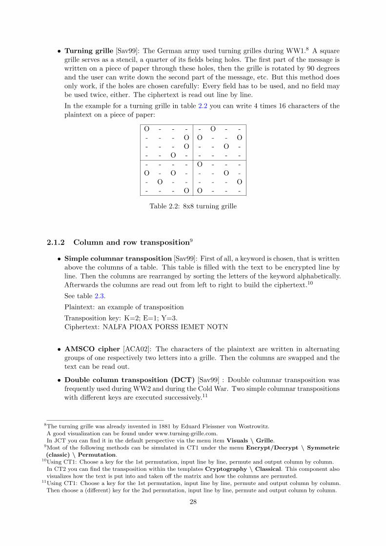
• Turning grille [Sav99]: The German army used turning grilles during WW1.8 A squaregrille serves as a stencil, a quarter of its fields being holes. The first part of the message iswritten on a piece of paper through these holes, then the grille is rotated by 90 degreesand the user can write down the second part of the message, etc. But this method doesonly work, if the holes are chosen carefully: Every field has to be used, and no field maybe used twice, either. The ciphertext is read out line by line.
In the example for a turning grille in table 2.2 you can write 4 times 16 characters of theplaintext on a piece of paper:
O - - - - O - -- - - O O - - O- - - O - - O -- - O - - - - -
- - - - O - - -O - O - - - O -- O - - - - - O- - - O O - - -
Table 2.2: 8x8 turning grille
2.1.2 Column and row transposition9
• Simple columnar transposition [Sav99]: First of all, a keyword is chosen, that is writtenabove the columns of a table. This table is filled with the text to be encrypted line byline. Then the columns are rearranged by sorting the letters of the keyword alphabetically.Afterwards the columns are read out from left to right to build the ciphertext.10
See table 2.3.
Plaintext: an example of transposition
Transposition key: K=2; E=1; Y=3.Ciphertext: NALFA PIOAX PORSS IEMET NOTN
• AMSCO cipher [ACA02]: The characters of the plaintext are written in alternatinggroups of one respectively two letters into a grille. Then the columns are swapped and thetext can be read out.
• Double column transposition (DCT) [Sav99] : Double columnar transposition wasfrequently used during WW2 and during the Cold War. Two simple columnar transpositionswith different keys are executed successively.11
8The turning grille was already invented in 1881 by Eduard Fleissner von Wostrowitz.A good visualization can be found under www.turning-grille.com.In JCT you can find it in the default perspective via the menu item Visuals \ Grille.
9Most of the following methods can be simulated in CT1 under the menu Encrypt/Decrypt \ Symmetric(classic) \ Permutation.
10Using CT1: Choose a key for the 1st permutation, input line by line, permute and output column by column.In CT2 you can find the transposition within the templates Cryptography \ Classical. This component alsovisualizes how the text is put into and taken off the matrix and how the columns are permuted.
11Using CT1: Choose a key for the 1st permutation, input line by line, permute and output column by column.Then choose a (different) key for the 2nd permutation, input line by line, permute and output column by column.
28

K E Y
a n ex a mp l eo f tr a ns p os i ti o n
Table 2.3: Simple columnar transposition
If the keys are different and long enough (at least each 20 characters), then this is even fortoday’s computer a real challenge.12
• Column transposition, General Luigi Sacco [Sav99]: The columns of a table arenumbered according to the letters of the keyword. The plaintext is entered line by line, inthe first line up to column number one, in the second line up to column number two, etc.Again, the ciphertext is read out in columns.
See table 2.4.
Plaintext: an example of transposition
C O L U M N1 5 2 6 3 4
an e xa m p l eo f t r a ns po s i ti o n
Table 2.4: Columnar transposition (General Luigi Sacco)
Ciphertext: ANAOS OIEMF PSOXP TINLR TEAN
• Column transposition, French army in WW1 [Sav99]: After executing a simplecolumnar transposition, diagonal rows are read out.
• Row transposition [Sav99]: The plaintext is divided into blocks of equal length and akeyword is chosen. Now the letters of the keyword are numbered and permutation is doneonly within each block according to this numbering.13
12MTC3 offers according challenges, for instancehttp://www.mysterytwisterc3.org/en/challenges/level-x/double-column-transposition andhttps://www.mysterytwisterc3.org/en/challenges/level-iii/double-column-transposition-reloaded-
part-113Using CT1: Choose a key for 1st permutation, input line by line, permute column by column and output line by
29

2.1.3 Further transposition algorithm ciphers
• Geometric figures [Goe14]: Write the message into a grille following one pattern andread it out using another.
• Union Route Cipher [Goe14]: The Union Route Cipher derives from Civil War. Thismethod does not rearrange letters of a given plaintext, but whole words. Particularlysensitive names and terms are substituted by codewords which are recorded in codebookstogether with the existing routes. A route determines the size of a grille and the patternthat is used to read out the ciphertext. In addition, a number of filler words is defined.
• Nihilist Transposition [ACA02]: Insert the plaintext into a square grille and writethe same keyword above the columns and next to the lines. As this keyword is sortedalphabetically, the contents of the grille are rearranged, too. Read out the ciphertext lineby line.
See table 2.5.
Plaintext: an example of transposition
W O R D S D O R S W
W a n e x a D s p o i sO m p l e o O e p l o mR f t r a n R a t r n fD s p o s i S n i o - tS t i o n - W x n e a a
Table 2.5: Nihilist transposition14
Ciphertext: SPOIS EPLOM ATRNF NIOTX NEAA
• Cadenus cipher [ACA02]: Cadenus is a form of columnar transposition that uses twokeywords.The 1st keyword is used to swap columns.The 2nd keyword is used to define the initial letter of each column: this 2nd keyword isa permutation of the used alphabet. This permutation is written on the left of the firstcolumn. Afterwards, each column is moved (wrap-around) so that it begins with the letter,which is in the same line as the key letter of the first keyword within the second keyword.Ciphertext is read out line by line.
See table 2.6.
Plaintext: cadenus is a form of columnar transposition using a keyword
Ciphertext:SAASR PIFIU LONNS KTGWN EDOOA TDNNU IISFA OMYOC ROUCM AERRS
line.In CT2 you can find the transposition within the templates Cryptography \ Classical. This component alsovisualizes the row wise transposition.
14After filling the matrix with the plaintext you get the left block. After switching rows and columns you get theright block
15Within the 2nd block of three chars those chars are printed bold which are at the top of the 3rd block afterapplying the 2nd key word.
30

K E Y E K Y E K Y
A c a d a c d s a aD e n u n e u s r pX s i s i s s i f iK a f o f a o u l oC r m o m r o n n sW f c o c f o k t gN l u m u l m w n eS n a r a n r d o oY t r a r t a a t dE n s p s n p n n uD o s i s o i i i sT t i o i t o f a oU n u s u n s m y oB i n g n i g c r oR a k e k a e u c mG y w o w y o a e rH r d - d r - r s -
Table 2.6: Cadenus cipher15
31
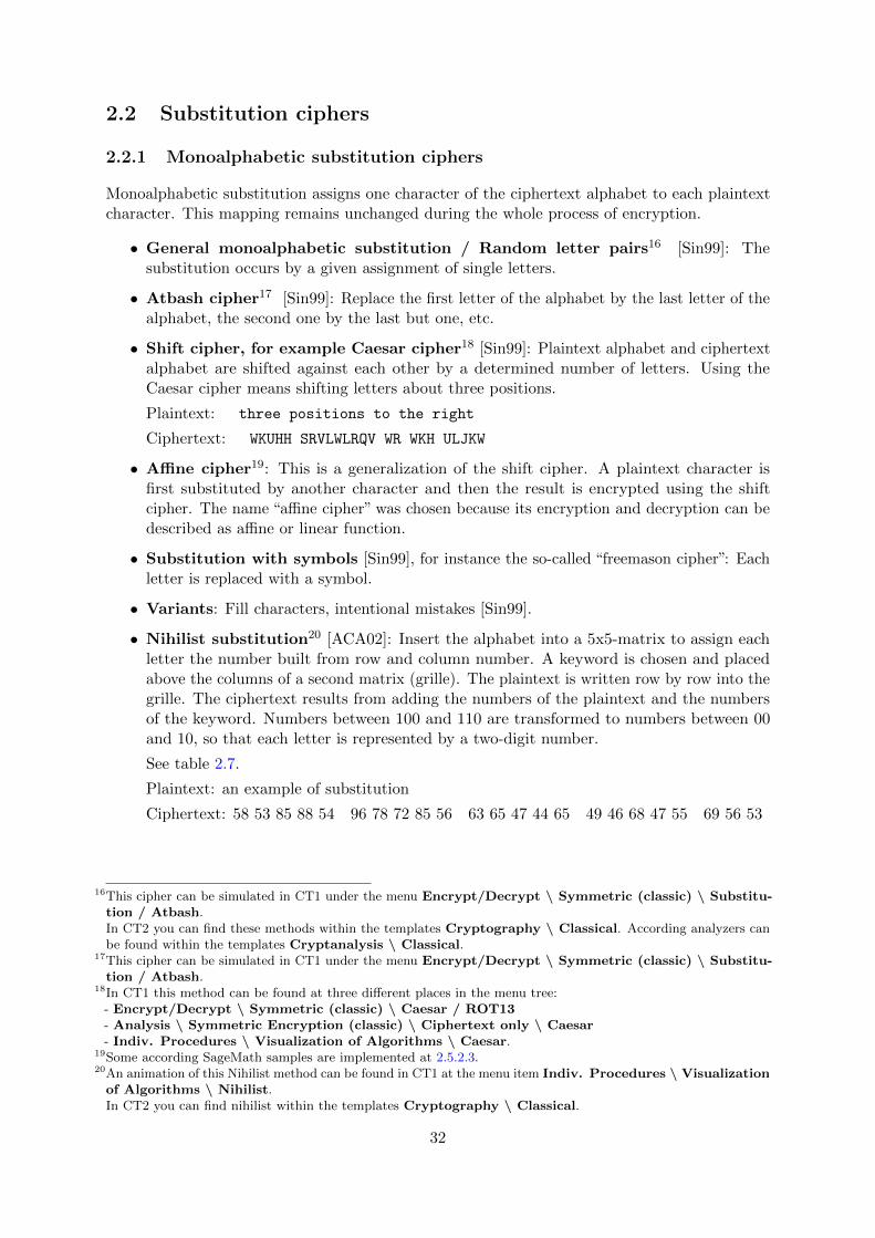
2.2 Substitution ciphers
2.2.1 Monoalphabetic substitution ciphers
Monoalphabetic substitution assigns one character of the ciphertext alphabet to each plaintextcharacter. This mapping remains unchanged during the whole process of encryption.
• General monoalphabetic substitution / Random letter pairs16 [Sin99]: Thesubstitution occurs by a given assignment of single letters.
• Atbash cipher17 [Sin99]: Replace the first letter of the alphabet by the last letter of thealphabet, the second one by the last but one, etc.
• Shift cipher, for example Caesar cipher18 [Sin99]: Plaintext alphabet and ciphertextalphabet are shifted against each other by a determined number of letters. Using theCaesar cipher means shifting letters about three positions.
Plaintext: three positions to the right
Ciphertext: WKUHH SRVLWLRQV WR WKH ULJKW
• Affine cipher19: This is a generalization of the shift cipher. A plaintext character isfirst substituted by another character and then the result is encrypted using the shiftcipher. The name “affine cipher” was chosen because its encryption and decryption can bedescribed as affine or linear function.
• Substitution with symbols [Sin99], for instance the so-called “freemason cipher”: Eachletter is replaced with a symbol.
• Variants: Fill characters, intentional mistakes [Sin99].
• Nihilist substitution20 [ACA02]: Insert the alphabet into a 5x5-matrix to assign eachletter the number built from row and column number. A keyword is chosen and placedabove the columns of a second matrix (grille). The plaintext is written row by row into thegrille. The ciphertext results from adding the numbers of the plaintext and the numbersof the keyword. Numbers between 100 and 110 are transformed to numbers between 00and 10, so that each letter is represented by a two-digit number.
See table 2.7.
Plaintext: an example of substitution
Ciphertext: 58 53 85 88 54 96 78 72 85 56 63 65 47 44 65 49 46 68 47 55 69 56 53
16This cipher can be simulated in CT1 under the menu Encrypt/Decrypt \ Symmetric (classic) \ Substitu-tion / Atbash.In CT2 you can find these methods within the templates Cryptography \ Classical. According analyzers canbe found within the templates Cryptanalysis \ Classical.
17This cipher can be simulated in CT1 under the menu Encrypt/Decrypt \ Symmetric (classic) \ Substitu-tion / Atbash.
18In CT1 this method can be found at three different places in the menu tree:- Encrypt/Decrypt \ Symmetric (classic) \ Caesar / ROT13- Analysis \ Symmetric Encryption (classic) \ Ciphertext only \ Caesar- Indiv. Procedures \ Visualization of Algorithms \ Caesar.
19Some according SageMath samples are implemented at 2.5.2.3.20An animation of this Nihilist method can be found in CT1 at the menu item Indiv. Procedures \ Visualization
of Algorithms \ Nihilist.In CT2 you can find nihilist within the templates Cryptography \ Classical.
32

Matrix
1 2 3 4 5
1 S U B T I2 O N A C D3 E F G H K4 L M P Q R5 V W X Y Z
Table
K E Y(35) (31) (54)
a n e(58) (53) (85)
x a m(88) (54) (96)
p l e(78) (72) (85)
o f s(56) (63) (65)
u b s(47) (44) (65)
t i t(49) (46) (68)
u t i(47) (55) (69)
o n(56) (53)
Table 2.7: Nihilist substitution
• Codes [Sin99]: In the course of time, codebooks were used again and again. A codebookassigns a codeword, a symbol or a number to every possible word of a message. Onlyif both parties hold identical codebooks and if the assignment of codewords to plaintextwords is not revealed, a successful and secret communication can take place.
• Nomenclator [Sin99]: A nomenclator refers to techniques that combine the use of acipher algorithm with a codebook. Often the encryption system is based upon a ciphertextalphabet. This alphabet is used to encrypt (via substitution) the bigger part of the message.Particularly frequent or top-secret words are replaced by a limited number of codewordsexisting besides the ciphertext alphabet.
• Map cipher [Thi99]: This method constitutes a combination of substitution and stegano-graphy21. Plaintext characters are replaced by symbols which are arranged in a mapfollowing certain rules.
• Straddling Checkerboard [Goe14]: A 3x10 matrix is filled with the letters of the usedalphabet and two arbitrary digits or special characters as follows: The different lettersof a keyword and the remaining characters are written into the grille. The columns arenumbered 0 to 9, the second and the third line are numbered 1 and 2. Each plaintextcharacter is replaced by the corresponding digit, respectively the corresponding pair of
21Instead of encrypting a message, pure steganography tries to conceal its existence.
33

digits. As “1” and “2” are the first digits of the possible two-digit-numbers, they are notused as single digits.
See table 2.8.
Plaintext: an example of substitution
0 1 2 3 4 5 6 7 8 9
K - - E Y W O R D A1 B C F G H I J L M N2 P Q S T U V X Z . /
Table 2.8: Straddling checkerboard with password “Keyword”
Ciphertext: 91932 69182 01736 12222 41022 23152 32423 15619
Besides, “1” and “2” are the most commonly used digits, but this feature is removed by thefollowing technique.
It is ostentatious, how often the numbers 1 and 2 appear, but this will be fixed with thefollowing version.
• Straddling Checkerboard, variant [Goe14]: This variant of the straddling checker-board was developed by Soviet spies during WW2. Ernesto (Che) Guevara and FidelCastro allegedly used this cipher for their secret communication.22 A grille is filled with thealphabet (number of columns = length of keyword), and two arbitrary digits are chosen asreserved to indicate the second and third line of a 3x10-matrix (see above). Now the grilleis traversed column by column and the single letters are transferred row by row into thematrix: For a faster encryption, the eight most common letters (ENIRSATO) are assignedthe digits from 0 to 9, the reserved 2 digits are not assigned. The remaining letters areprovided with combinations of digits one after another and are inserted into the grille.
See table 2.9.
Plaintext: an example of substitution
Ciphertext: 04271 03773 33257 09343 29181 34185 4
– Che Guevara cipher: A special variant is the cipher used by Che Guevara (withan additional substitution step and a slightly changed checkerboard):
∗ The seven most frequent letters in Spanish are distributed in the first row.
∗ Four instead of three rows are used.
∗ So one could encrypt 10 ∗ 4− 4 = 36 different characters.
• Tri-Digital cipher [ACA02]: A keyword with ten letters is used to create a numeric keyby numbering its letters corresponding to their alphabetical order. This key is written
22In addition, Che Guevara used for his communication with Fidel Castro also a one-time pad.See part 3 of the series RSA & Co. at school: Modern cryptology, old mathematics, and subtle protocols: [WLS99],p. 52.Unfortunately these are currently only available in German.
34
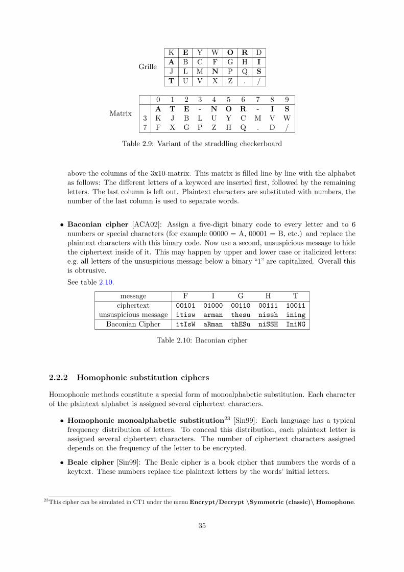
Grille
K E Y W O R D
A B C F G H I
J L M N P Q S
T U V X Z . /
Matrix
0 1 2 3 4 5 6 7 8 9
A T E - N O R - I S3 K J B L U Y C M V W7 F X G P Z H Q . D /
Table 2.9: Variant of the straddling checkerboard
above the columns of the 3x10-matrix. This matrix is filled line by line with the alphabetas follows: The different letters of a keyword are inserted first, followed by the remainingletters. The last column is left out. Plaintext characters are substituted with numbers, thenumber of the last column is used to separate words.
• Baconian cipher [ACA02]: Assign a five-digit binary code to every letter and to 6numbers or special characters (for example 00000 = A, 00001 = B, etc.) and replace theplaintext characters with this binary code. Now use a second, unsuspicious message to hidethe ciphertext inside of it. This may happen by upper and lower case or italicized letters:e.g. all letters of the unsuspicious message below a binary “1” are capitalized. Overall thisis obtrusive.
See table 2.10.
message F I G H T
ciphertext 00101 01000 00110 00111 10011
unsuspicious message itisw arman thesu nissh ining
Baconian Cipher itIsW aRman thESu niSSH IniNG
Table 2.10: Baconian cipher
2.2.2 Homophonic substitution ciphers
Homophonic methods constitute a special form of monoalphabetic substitution. Each characterof the plaintext alphabet is assigned several ciphertext characters.
• Homophonic monoalphabetic substitution23 [Sin99]: Each language has a typicalfrequency distribution of letters. To conceal this distribution, each plaintext letter isassigned several ciphertext characters. The number of ciphertext characters assigneddepends on the frequency of the letter to be encrypted.
• Beale cipher [Sin99]: The Beale cipher is a book cipher that numbers the words of akeytext. These numbers replace the plaintext letters by the words’ initial letters.
23This cipher can be simulated in CT1 under the menu Encrypt/Decrypt \Symmetric (classic)\ Homophone.
35

• Grandpre cipher [Sav99]: A square grille with 10 columns (other layouts are possible,too) is filled with ten words. The initial letters should result in an eleventh word. Ascolumns and rows are numbered from 0 to 9, letters can be replaced by two-digit numbers.It is obvious that with the table having a hundred fields, most letters can be representedby more than one number. You should keep in mind that those ten words have to containall letters of the plaintext alphabet.
• Book cipher: The words of a message are substituted by triples “page-line-position”.This method requires a detailed agreement of which book to use, especially regarding theedition (layout, error correction, etc.).
2.2.3 Polygraphic substitution ciphers
Polygraphic techniques do not work by replacing single characters, but by replacing whole groupsof characters. In most cases, these groups are diagrams, trigrams or syllables.
• “Great Chiffre” [Sin99]: This cipher was used by Louis XIV. and was not solved untilthe end of the nineteenth century. Cryptograms consisted of 587 different numbers, everynumber representing a syllable. The inventors of the “Great Chiffre” (Rossignol, fatherand son) constructed additional traps to increase security. For example, a number couldassign a different meaning to or delete the preceding one.
• Playfair cipher24 [Sin99]: A 5x5-matrix is filled with the plaintext characters. Forexample, the different letters of a keyword are inserted first, followed by the remainingletters. The plaintext is divided into pairs, these digraphs are encrypted using the followingrules:
1. If both letters can be found in the same column, they are replaced by the lettersunderneath.
2. If both letters can be found in the same row, take the letters to their right.
3. If both letters of the digraph are in different columns and rows, the replacementletters are obtained by scanning along the row of the first letter up to the columnwhere the other letter occurs and vice versa.
4. Double letters are treated by special rules, if they appear in one digraph. They canbe separated by a filler, for example.
See table 2.11.
Unformated Plaintext: plaintext letters are encrypted in pairsFormated Plaintext: pl ai nt ex tl et te rs ar ee ncrypted in pairsFormated Plaintext: pl ai nt ex tl et te rs ar ex en cr yp te di np ai rs
Ciphertext: SHBHM UWUZF KUUKC MBDWU DURDA VUKBG PQBHC M
• Trigraphic Playfair: A 5x5-matrix is filled with the alphabet (see above) and theplaintext is divided into trigraphs. Trigraphs are encrypted according to the followingrules:
24In CT1 you can call this method under the menu Encrypt/Decrypt \ Symmetric (classic) \ Playfair.In CT2 you can find the Playfair within the templates Cryptography \ Classical.In JCT you can find it in the default perspective via the menu item Algorithms \ Classic \ Playfair.
36

K E Y W O
R D A B C
F G H I L
M N P Q S
T U V X Z
Table 2.11: 5x5 Playfair matrix with password “Keyword”
1. Three equal letters are substituted by three equal letters. It is the letter on the rightunderneath the original letter.
2. A trigraph with two different letters is encrypted like a digraph in Playfair.
3. If a trigraph contains three different characters, very complex rules come into effect.See [Sav99]
• Substituting digraphs by symbols [Sav99]: Giovanni Battista della Porta, 15th century.He created a 20x20-matrix that contained one symbol for every possible combination ofletters (his alphabet did not comprise more than twenty letters).
• Four square cipher [Sav99]: This method is similar to Playfair, because it is based on asystem of coordinates whose four quadrants are each filled with the alphabet. The layoutof letters can differ from quadrant to quadrant. To encipher a message, act in the followingway: Look up the first plaintext letter in the first quadrant and the second one in the thirdquadrant. These two letters are opposite corners of a rectangle and the ciphertext letterscan be found in quadrant number two and four.
See table 2.12.
Plaintext: plaintext letters are encrypted in pairs
d w x y m E P T O Lr q e k i C V I Q Zu v h p s R M A G Ua l b z n F W Y H Sg c o f t B N D X K
Q T B L E v q i p gZ H N D X s t u o hP M I Y C n r d x yV S K W O b l w m fU A F R G c z k a e
Table 2.12: Four square cipher
Ciphertext: MWYQW XQINO VNKGC ZWPZF FGZPM DIICC GRVCS
• Two square cipher [Sav99]: The two square cipher resembles the four square cipher, butthe matrix is reduced to two quadrants. Are both letters of the digraph part of the samerow, they are just exchanged. Otherwise, the plaintext letters are considered as oppositecorners of a rectangle and substituted by the other vertices. Quadrants can be arrangedhorizontal and vertical.
37

• Tri square cipher [ACA02]: Three quadrants are filled with the same alphabet. Thefirst plaintext letter is looked up in the first quadrant and can be encrypted with everyletter of that column. The second plaintext letter is looked up in the second quadrant(diagonally across) and can be encrypted with every letter of that row. Between these twociphertext characters, the letter at the intersection point is set.
• Dockyard cipher [Sav99]: Used by the German navy during WW2.
2.2.4 Polyalphabetic substitution ciphers
Concerning polyalphabetic substitution, the assignment of ciphertext characters to plaintextcharacters is not static, but changes during the process of encryption (depending on the key).
• Vigenere25 [Sin99]: Each plaintext character is encrypted with a different ciphertextalphabet that is determined by the characters of a keyword (the so-called Vigenere tableauserves auxiliary means). If the plaintext is longer than the key, the latter is repeated.
See table 2.13.
Plaintext: the alphabet is changing
Key: KEY KEYKEYKE YK EYKEYKEY
Ciphertext: DLC KPNREZOX GC GFKRESRE
- A B C D E F G H I J K L M N O P Q R S T U V W X Y Z
A A B C D E F G H I J K L M N O P Q R S T U V W X Y ZB B C D E F G H I J K L M N O P Q R S T U V W X Y Z AC C D E F G H I J K L M N O P Q R S T U V W X Y Z A BD D E F G H I J K L M N O P Q R S T U V W X Y Z A B CE E F G H I J K L M N O P Q R S T U V W X Y Z A B C DF F G H I J K L M N O P Q R S T U V W X Y Z A B C D EG G H I J K L M N O P Q R S T U V W X Y Z A B C D E FH H I J K L M N O P Q R S T U V W X Y Z A B C D E F GI I J K L M N O P Q R S T U V W X Y Z A B C D E F G HJ J K L M N O P Q R S T U V W X Y Z A B C D E F G H IK K L M N O P Q R S T U V W X Y Z A B C D E F G H I J... ... ...
Table 2.13: Vigenere tableau
– Interrupted key: The key is not repeated continuously, but starts again with everynew word of the message.
– Autokey26 [Sav99]: After using the agreed key, use the message itself as a key. Seetable 2.14.
25In CT1 you can call this method under the menu Encrypt/Decrypt \ Symmetric (classic) \ Vigenere.In CT2 you can find this method within the templates Cryptography \ Classical.In JCT you can find it in the default perspective via the menu item Algorithms \ Classic \ Vigenere.
26In CT2 you can find this method within the templates Cryptography \ Classical.In JCT you can find it in the default perspective via the menu item Algorithms \ Classic \ Autokey Vigenere.
38

Plaintext: the alphabet is changing
Key: KEY THEALPHA BE TISCHANG
Ciphertext: DLC TSTHLQLT JW VPSPNIAM
Table 2.14: Autokey variant of Vigenere
– Progressive key [Sav99]: The key changes during the process of encryption. Withevery repetition, the characters of the keyword are shifted about one position. “KEY”becomes “LFZ”.
– Gronsfeld [Sav99]: Variant of Vigenere that uses a numeric key.
– Beaufort [Sav99]: Variant of Vigenere, the key is subtracted, not added. Theciphertext alphabets may be written backwards.
– Porta [ACA02]: Variant of Vigenere with only 13 alphabets. As a consequence, twoletters of the keyword are assigned the same ciphertext alphabet and the first andthe second half of the alphabet are reciprocal.
– Slidefair [ACA02]: This method can be used as a variant of Vigenere, Gronsfeld orBeaufort. Slidefair does encrypt digraphs according to the following rules: Look upthe first letter in the plaintext alphabet above the tableau. Then look up the secondone in the row belonging to the corresponding keyword letter. These two letters makeup opposite corners of an imaginary rectangle. The letters at the two remainingcorners substitute the digraph.
• One-time pad (OTP)27,28: This is a major concept: A sequence of bytes is XORedbyte-by-byte to the plaintext. This is a generalization of Vigenere’s mechanism and it wasthe first information theoretically secure scheme (see chapter 1.1 “Security definitions andthe importance of cryptology”).
To fulfill this claim the pad must be random and it must be used only once (to eliminateany semblance of pattern from the ciphertext).Reason: Given ciphertext C, plaintext P, pad K and two plaintexts encrypted with thesame key: C1 = P1 ⊕ K; C2 = P2 ⊕ K;Thus, C1 ⊕ C2 = (P1 ⊕ K) ⊕ (P2 ⊕ K) = P1 ⊕ P2;which effectively could leak the plaintexts.29
• Superposition (some variants of the OTP)
– Running-key cipher: A keytext (for example out of a book) is added to theplaintext.
– Superposition with numbers: A sequence or a number of sufficient length (forexample pi) is added.
27On a big scale OTPs have been successfully analyzed by Americans and British during the “Venona” project –because of wrong usage by the soviet spies. See https://en.wikipedia.org/wiki/Venona_project.
28CT1 offers this method under the menu Encrypt/Decrypt \ Symmetric (classic) \ Vernam / OTP.In CT2 you can find this method within the templates Cryptography \ Classical.In JCT you can find it in the default perspective via the menu item Algorithms \ Classic \ XOR.In chapter 8.3.1 you find a detailed description of the OTP as bitstream cipher and its implementation in SageMath.
29In JCT you can play with an automatic cryptanalysis of running-key ciphertexts using the Viterbi analysis underthe menu Visuals \ Viterbi. You can see how astonishing it is, if you get little by little from XORed ciphertextsor XORed plaintexts both original plaintexts.
39

• Phillips cipher [ACA02]: The alphabet is filled into a square table with 5 columns. Sevenmore tables are generated by first shifting the first row one position towards the bottom,then shifting the second row towards the bottom. The plaintext is divided into blocks offive which are encrypted with one matrix each. Letters are substituted by the ones ontheir right and underneath.
• Ragbaby cipher [ACA02]: Construct an alphabet with 24 characters. Then number theplaintext characters, starting the numeration of the first word with “1”, the numeration ofthe second one with “2” and so forth. Number 25 corresponds to number 1. Each letter ofthe message is encrypted by shifting it the corresponding positions to the right.
See table 2.15.
alphabet: KEYWORDABCFGHILMNPSTUVXZ
Plaintext: t h e a l p h a b e t i s c h a n g i n gNumbering: 1 2 3 2 3 4 5 6 7 8 9 3 4 4 5 6 7 8 9 10 11Ciphertext: U L O C P V P I M C O N X I P I Z T X Y X
Table 2.15: Ragbaby cipher
40

2.3 Combining substitution and transposition
In the history of cryptography one often comes across combinations of the previous mentionedmethods.
• ADFG(V)X30 [Sin99]: ADFG(V)X-encryption was developed in Germany during WW1.The alphabet is filled into a 5x5 or 6x6 matrix, and columns and rows are marked withthe letters ADFGX and V, depending on the size of the grille. Each plaintext character issubstituted by the corresponding pair of letters. Finally, a (row-) transposition cipher isperformed on the resulting text.
• Fractionation [Sav99]: Generic term for all kinds of methods that encrypt one plaintextcharacter by several ciphertext characters and then apply a transposition cipher to thisciphertext so that ciphertext characters originally belonging to each other are separated.
– Bifid/Polybius square/checkerboard [Goe14]: Bifid encryption is the basic formof fractionation. A 5x5 matrix is filled with the plaintext alphabet (see Playfairencryption), rows and columns are numbered, so that each plaintext character canbe substituted by a pair of digits. Mostly the plaintext is divided into blocks ofequal length. The length of blocks (here 5) is another configuration parameter of thiscipher. Block-by-block all line numbers are read out first, followed by all numbersnaming the columns. To obtain the ciphertext, the digits are pairwise transformedinto letters again. The numbers can be any permutation of (1,2,3,4,5), which is onekey of configuration parameter of this cipher. Instead of numbering rows and columns,a keyword can be used, too.
See table 2.16.
2 4 5 1 3
1 K E Y W O4 R D A B C2 F G H I L3 M N P Q S5 T U V X Z
Plaintext: combi nings ubsti tutio nandt ransp ositi
Rows: 41342 32323 54352 55521 34345 44333 13252
Columns: 33211 41443 41321 24213 45442 25435 33121
Table 2.16: Bifid cipher
41342 32323 54352 55521 34345 44333 13252 33211 41443 41321 24213 45442 2543533121
Ciphertext: BNLLL UPHVI NNUCS OHLMW BDNOI GINUR HCZQI
– Trifid [Sav99]: 27 characters (alphabet + 1 special character) may be represented bya triple consisting of the digits 1 to 3. The message to be encrypted is divided into
30In CT1 you can call this method under the menu Encrypt/Decrypt \ Symmetric (classic) \ ADFGVX.In CT2 you can find this method within the templates Cryptography \ Classical.
41
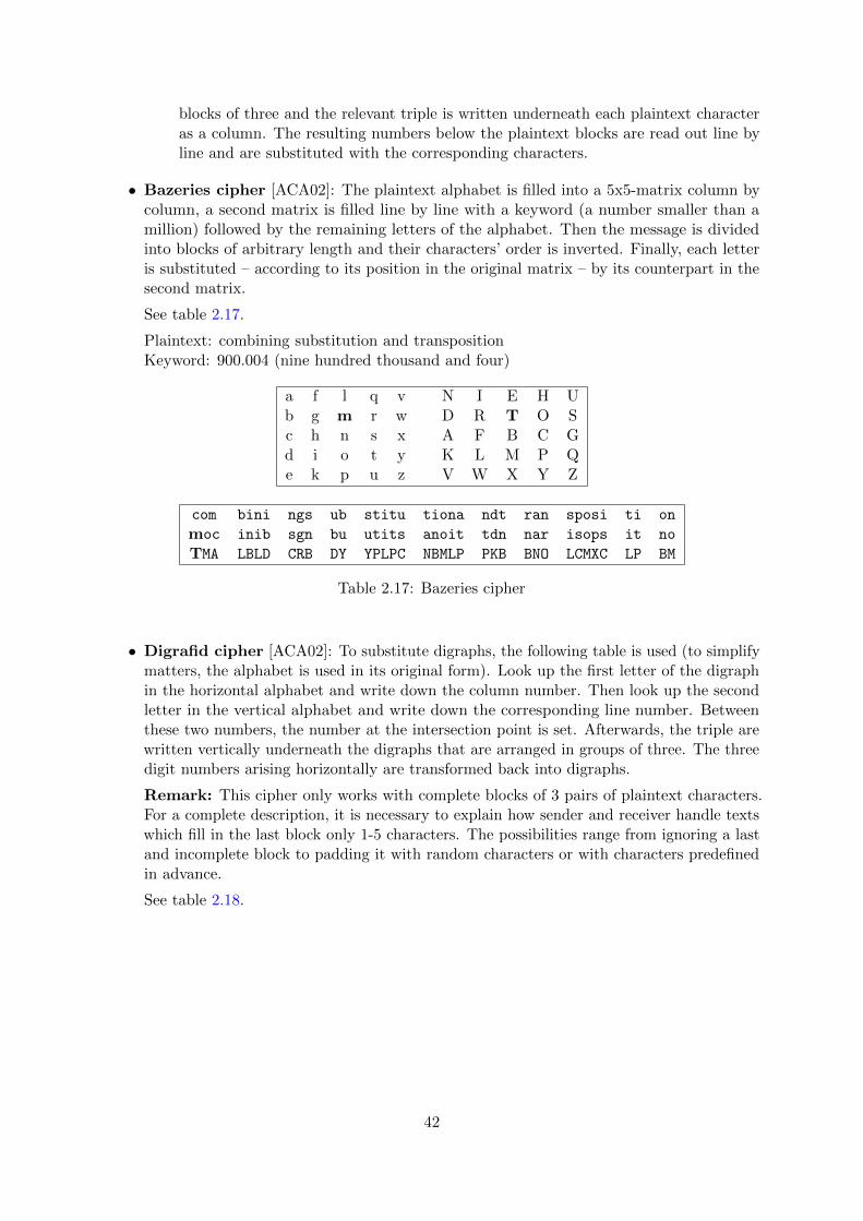
blocks of three and the relevant triple is written underneath each plaintext characteras a column. The resulting numbers below the plaintext blocks are read out line byline and are substituted with the corresponding characters.
• Bazeries cipher [ACA02]: The plaintext alphabet is filled into a 5x5-matrix column bycolumn, a second matrix is filled line by line with a keyword (a number smaller than amillion) followed by the remaining letters of the alphabet. Then the message is dividedinto blocks of arbitrary length and their characters’ order is inverted. Finally, each letteris substituted – according to its position in the original matrix – by its counterpart in thesecond matrix.
See table 2.17.
Plaintext: combining substitution and transpositionKeyword: 900.004 (nine hundred thousand and four)
a f l q v N I E H Ub g m r w D R T O Sc h n s x A F B C Gd i o t y K L M P Qe k p u z V W X Y Z
com bini ngs ub stitu tiona ndt ran sposi ti on
moc inib sgn bu utits anoit tdn nar isops it no
TMA LBLD CRB DY YPLPC NBMLP PKB BNO LCMXC LP BM
Table 2.17: Bazeries cipher
• Digrafid cipher [ACA02]: To substitute digraphs, the following table is used (to simplifymatters, the alphabet is used in its original form). Look up the first letter of the digraphin the horizontal alphabet and write down the column number. Then look up the secondletter in the vertical alphabet and write down the corresponding line number. Betweenthese two numbers, the number at the intersection point is set. Afterwards, the triple arewritten vertically underneath the digraphs that are arranged in groups of three. The threedigit numbers arising horizontally are transformed back into digraphs.
Remark: This cipher only works with complete blocks of 3 pairs of plaintext characters.For a complete description, it is necessary to explain how sender and receiver handle textswhich fill in the last block only 1-5 characters. The possibilities range from ignoring a lastand incomplete block to padding it with random characters or with characters predefinedin advance.
See table 2.18.
42
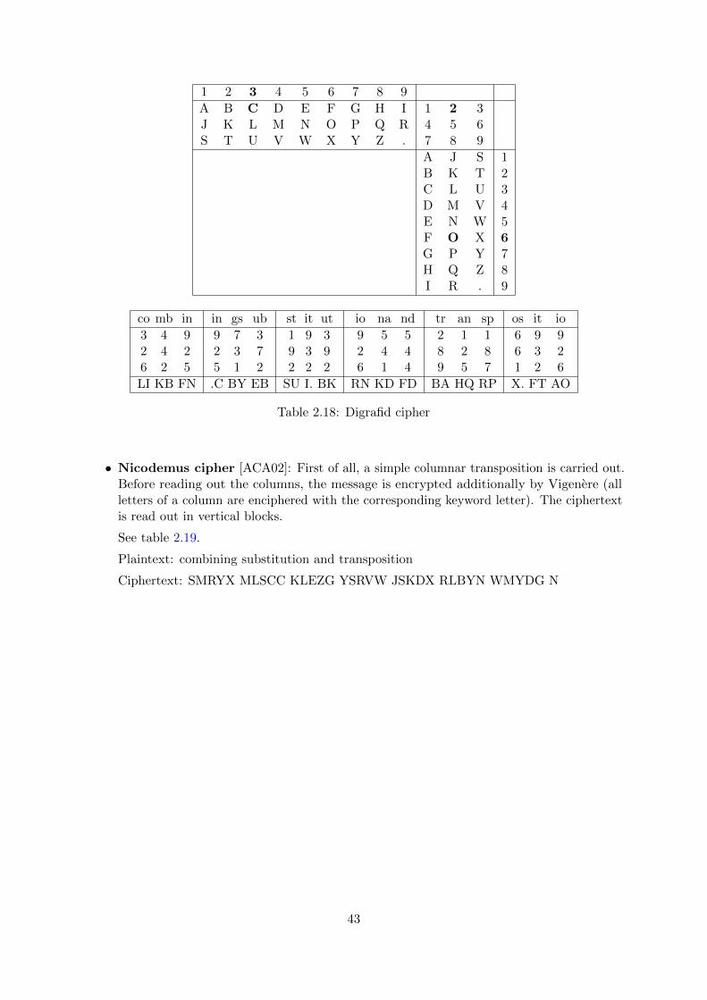
1 2 3 4 5 6 7 8 9
A B C D E F G H I 1 2 3J K L M N O P Q R 4 5 6S T U V W X Y Z . 7 8 9
A J S 1B K T 2C L U 3D M V 4E N W 5F O X 6G P Y 7H Q Z 8I R . 9
co mb in in gs ub st it ut io na nd tr an sp os it io
3 4 9 9 7 3 1 9 3 9 5 5 2 1 1 6 9 92 4 2 2 3 7 9 3 9 2 4 4 8 2 8 6 3 26 2 5 5 1 2 2 2 2 6 1 4 9 5 7 1 2 6
LI KB FN .C BY EB SU I. BK RN KD FD BA HQ RP X. FT AO
Table 2.18: Digrafid cipher
• Nicodemus cipher [ACA02]: First of all, a simple columnar transposition is carried out.Before reading out the columns, the message is encrypted additionally by Vigenere (allletters of a column are enciphered with the corresponding keyword letter). The ciphertextis read out in vertical blocks.
See table 2.19.
Plaintext: combining substitution and transposition
Ciphertext: SMRYX MLSCC KLEZG YSRVW JSKDX RLBYN WMYDG N
43
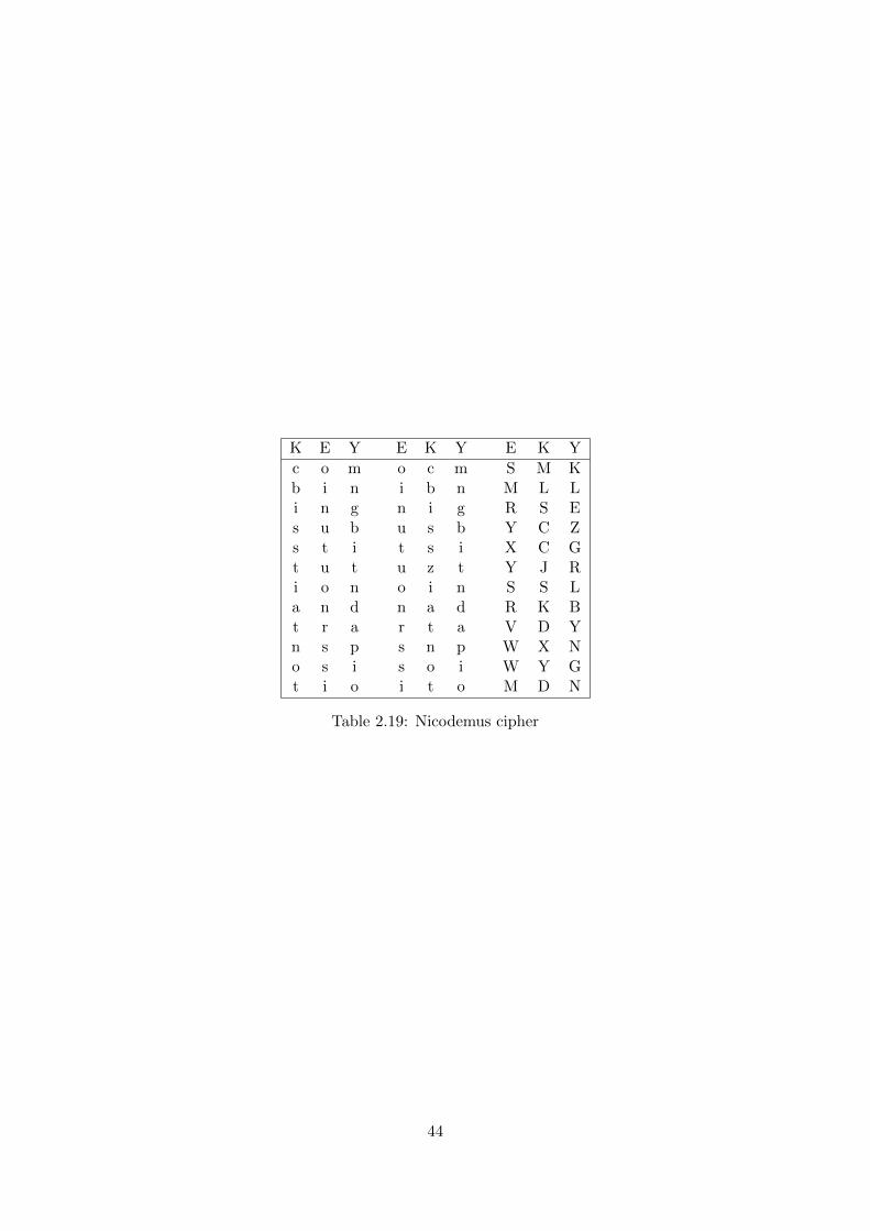
K E Y E K Y E K Y
c o m o c m S M Kb i n i b n M L Li n g n i g R S Es u b u s b Y C Zs t i t s i X C Gt u t u z t Y J Ri o n o i n S S La n d n a d R K Bt r a r t a V D Yn s p s n p W X No s i s o i W Y Gt i o i t o M D N
Table 2.19: Nicodemus cipher
44
• Double column transposition (DCT) / “Granit E160” [Dro15] : Granit is a 2-stepcipher. The second step is the double colum transposition; in the first step before, thecleartext is substituted by a sequence of digits using a codebook and a matrix (a variantof the Polybios square).
The Granit cipher was used for instance by the spy Guenter Guillaume for his communica-tion with the Ministry of State Security of the former GDR until about 1960.31
31MTC3 offers according challenges. If you enter at https://www.mysterytwisterc3.org/en/challenges/the-
four-levels?showAll=1 in your browser the search item “Granit”, you’ll find 6 challenges about it.A detailed 20-page description about the Granit cipher can be found at:https://www.mysterytwisterc3.org/images/challenges/mtc3-drobick-01-doppelwuerfel-01-en.pdf
45

2.4 Further methods
• “Pinprick encryption” [Sin99]: For centuries, this simple encryption method has beenput into practice for different reasons (actually steganography). During the Victorian Age,for example, small holes underneath letters in newspaper articles marked the characters ofa plaintext, as sending a newspaper was much more cheaper than the postage on a letter.
• Stencil: Stencils (Cardboard with holes) are also known as “Cardinal-Richelieu-Key”.Sender and receiver have to agree upon a text. Above this text, a stencil is laid and theletters that remain visible make up the ciphertext.
• Card games [Sav99]: The key is created by means of a pack of cards and rules that areagreed upon in advance. All methods mentioned in this paragraph are designed as paperand pencil methods, i.e. they are applicable without electronic aid. A pack of cards isunsuspicious to outsiders, shuffling the deck provides a certain amount of coincidence,cards can be transformed into numbers easily and a transposition cipher can be carriedout without any further aid.
– Solitaire cipher (Bruce Schneier)32 [Sch99]: Sender and receiver have to own adeck of cards shuffled in the same manner. A key stream is generated that has toconsist of as many characters as the message to be encrypted.
The algorithm to generate the key is based on a shuffled deck of 54 cards (Ace, 2 - 10,jack, queen, king in four suits and two jokers). The pack of cards is held face up:
1. Swap the first joker with the card beneath it.
2. Move the second joker two cards down.
3. Now swap the cards above the first joker with those below the second one.
4. Look at the bottom card and convert it into a number from 1 to 53 (bridgeorder of suits: clubs, diamonds, hearts, spades; joker = 53). Write down thisnumber and count down as many cards starting with the top card. These cardsare swapped with the remaining cards, only the bottom card remains untouched.
5. Look at the top card and convert it into a number, too. Count down as manycards starting with the top card.
6. Write down the number of the following card. This card is converted into yourfirst keystream character. As we need numbers from 1 to 26 to match the lettersof our alphabet, clubs and hearts correspond to the numbers 1 to 13, diamondsand spades to 14 to 26. If your output card is a joker, start again.
For each keystream character you like to generate, these six steps have to be carriedout. This procedure is – manually – very lengthy (4 h for 300 characters, dependenton your exercise) and requires high concentration.
Encryption takes place by addition modulo 26. Encryption is relatively fast comparedto the key stream generation.
This P&P cipher creates a key stream which is so good, that even nowadays it is hardto crack the cipher if you don’t know the originally sorted card deck (ciphertext-onlyattack).
32In CT1 you can call this method under the menu Encrypt/Decrypt \ Symmetric (classic) \ Solitaire.In CT2 you can find this method within the templates Cryptography \ Classical and Cryptanalysis \Classical.
46

– Mirdek cipher (Paul Crowley) [Cro00]: Even though this method is quite com-plicated, the author provides a very good example to illustrate the procedure.
– Playing Card cipher (John Savard) [Sav99]: This algorithm uses a shuffled deckof 52 cards (no joker). Separate rules describe how to shuffle the deck. A keystreamis created via the following steps:
1. The pack of cards lies in front of the user, top down. Cards are turned up anddealt out in a row until the total of the cards is 8 or more.
2. If the last card dealt out is a J, Q or K, write down its value, otherwise writedown the sum of the cards dealt out (a number between 8 and 17). In a secondrow, deal out that number of cards.
3. The remaining cards are dealt out in rows under the second row. The first oneends under the lowest card of the top row, the second one under the next lowestcard, and so on. If there are two identical cards, red is lower than black.
4. The cards dealt out under step 3 are collected column by column, starting withthe column under the lowest card. The first card that is picked up becomes thebottom card (face up).
5. The cards dealt out in step 1 and 2 are picked up, beginning with the last card.
6. The deck is turned over, the top card is now the bottom card (face down).Afterwards, steps 1 to 6 are repeated twice.
To generate a keystream character, write down the first card not being J, Q or K.Count down that number of cards. The card selected has to be between 1 and 10.Now repeat these steps beginning with the last card. These two numbers are addedand the last digit of the sum is your keystream character.
• VIC cipher [Sav99]: This is a highly complicated but relatively secure paper and pencilmethod. It has been developed and applied by Soviet spies. Amongst other things, theuser had to create ten pseudo-random numbers out of a date, the first words of a sentenceand any five-digit number. A straddling checkerboard is part of the encryption, too. Adetailed description can be found under [Sav99].
47

2.5 Appendix: Examples using SageMath
In the following section some classic ciphers are implemented using the open source computeralgebra system SageMath.33 The code was tested with SageMath version 5.3. All ciphers areexplained in chapter 2 (“Paper and Pencil Encryption Methods”).
To make the sample code34 of the ciphers easier to understand, we used the structure and thenaming conventions shown in the Figure 2.1 below:
• Encryption consists of the two steps encoding and enciphering.
– Encoding adapts the letters in the given plaintext P to the case defined in the givenalphabet, and all non-alphabet characters are filtered out.
– Enciphering creates the ciphertext C.
• Decryption also consists of two steps: deciphering and decoding.
– Decoding is only necessary if the symbols in the alphabet are not ASCII characters.
DEC
RYPT
ION
ENCR
YPTI
ON
Plaintext P
Message msg
Ciphertext C
Decrypted Ciphertext DC
encoding(get rid of non-alphabetcharacters)
enciphering
deciphering
Decoded DecryptedCiphertext DDC
decoding
Figure 2.1: Structure and naming convention of the SageMath cipher code examples
33A first introduction to the CAS SageMath can be found in the appendix A.7.34Further examples with SageMath concerning classic crypto methods can be found e.g.:
- as PDF in http://doc.sagemath.org/pdf/en/reference/cryptography/cryptography.pdf
- as HTML under http://doc.sagemath.org/html/en/reference/cryptography/index.html
- at http://doc.sagemath.org/html/en/reference/cryptography/sage/crypto/classical.html
- in the thesis of Minh Van Nguyen [Ngu09]
48

2.5.1 Transposition ciphers
Transposition ciphers are implemented in the SageMath class
sage.crypto.classical.TranspositionCryptosystem
To construct and work with a transposition cipher, we first need to determine the alphabet thatcontains the symbols used to build the space of our plaintext and ciphertext. Typically, thisalphabet will be the upper-case letters of the English alphabet, which can be accessed via thefunction
sage.monoids.string_monoid.AlphabeticStrings
We then need to decide on the block length of a block permutation, which is the length of therow vector to be used in the simple columns transposition. This row vector is our key, and itspecifies a permutation of a plaintext.
The following first example of transposition ciphers has block length 14, and the key is buildin a way, that every letter in the plaintext is shifted to the right by two characters, with wraparound at the end of the block. That is the encryption process. The decryption process isshifting each letter of the ciphertext to the left by 14− 2 = 12.
SageMath sample 2.1 Simple transposition by shifting (key and inverse key explicitly given)sage: # transposition cipher using a block length of 14
sage: T = TranspositionCryptosystem(AlphabeticStrings(), 14)
sage: # given plaintext
sage: P = "a b c d e f g h i j k l m n"
sage: # encryption key
sage: key = [3, 4, 5, 6, 7, 8, 9, 10, 11, 12, 13, 14, 1, 2]
sage:
sage: # encode plaintext (get rid of non-alphabet chars, convert lower-case to upper-case)
sage: msg = T.encoding(P)
sage: # encrypt plaintext by shifting to the left by 2 letters (do it in two steps)
sage: E = T(key)
sage: C = E(msg); C
CDEFGHIJKLMNAB
sage:
sage: # decrypt ciphertext by shifting to the left by 12 letters
sage: keyInv = [13, 14, 1, 2, 3, 4, 5, 6, 7, 8, 9, 10, 11, 12]
sage: D = T(keyInv)
sage: D(C)
ABCDEFGHIJKLMN
sage:
sage: # Representation of key and inverse key as permutations
sage: E
(1,3,5,7,9,11,13)(2,4,6,8,10,12,14)
sage: D
(1,13,11,9,7,5,3)(2,14,12,10,8,6,4)
49

The second example of transposition ciphers is also a simple shifting column transposition.But now the code is a little bit more automated: The keys are generated from the shift parameter.
SageMath sample 2.2 Simple transposition by shifting (key and inverse key constructed with“range”)sage: # transposition cipher using a block length of 14, code more variable
sage: keylen = 14
sage: shift = 2
sage: A = AlphabeticStrings()
sage: T = TranspositionCryptosystem(A, keylen)
sage:
sage: # construct the plaintext string from the first 14 letters of the alphabet plus blanks
sage: # plaintext = "A B C D E F G H I J K L M N"
sage: A.gens()
(A, B, C, D, E, F, G, H, I, J, K, L, M, N, O, P, Q, R, S, T, U, V, W, X, Y, Z)
sage: P=’’
sage: for i in range(keylen): P=P + " " + str(A.gen(i))
....:
sage: P
’ A B C D E F G H I J K L M N’
sage:
sage: # encryption key
sage: # key = [3, 4, 5, 6, 7, 8, 9, 10, 11, 12, 13, 14, 1, 2]
sage: key = [(i+shift).mod(keylen) + 1 for i in range(keylen)]; key
[3, 4, 5, 6, 7, 8, 9, 10, 11, 12, 13, 14, 1, 2]
sage:
sage: # encode plaintext (get rid of non-alphabet chars)
sage: msg = T.encoding(P)
sage: # encrypt plaintext by shifting to the left by 2 letters (do it in one step)
sage: C = T.enciphering(key, msg); C
CDEFGHIJKLMNAB
sage:
sage: # decrypt ciphertext by shifting to the left by 12 letters
sage: # keyInv = [13, 14, 1, 2, 3, 4, 5, 6, 7, 8, 9, 10, 11, 12]
sage: shiftInv=keylen-shift;
sage: keyInv = [(i+shiftInv).mod(keylen) + 1 for i in range(keylen)]; keyInv
[13, 14, 1, 2, 3, 4, 5, 6, 7, 8, 9, 10, 11, 12]
sage: DC = T.enciphering(keyInv, C); DC
ABCDEFGHIJKLMN
sage:
sage: # decryption using the "deciphering method with key" instead of "enciphering with keyInv"
sage: # using the deciphering method requires to change the type of the variable key
sage: DC = T.deciphering(T(key).key(), C); DC
ABCDEFGHIJKLMN
sage:
sage: # representation of key and inverse key as permutations
sage: T(key)
(1,3,5,7,9,11,13)(2,4,6,8,10,12,14)
sage: T(key).key()
(1,3,5,7,9,11,13)(2,4,6,8,10,12,14)
sage: T(keyInv)
(1,13,11,9,7,5,3)(2,14,12,10,8,6,4)
50

In the third example of transposition ciphers we use an arbitrary permutation as key inthe encryption and decryption processes in order to scramble the characters within each block(block length = number of columns in a simple column transposition). If the block length isn, then the key must be a permutation on n symbols. The following example uses the methodrandom_key() of the class TranspositionCryptosystem. Each call to random_key() producesa different key. Note that therefore your results (key and ciphertext) may be different from thefollowing example.
SageMath sample 2.3 Simple column transposition with randomly generated (permutation)keysage: # Remark: Enciphering here requires, that the length of msg is a multiple of keylen
sage: keylen = 14 # length of key
sage: A = AlphabeticStrings()
sage: T = TranspositionCryptosystem(A, keylen); T
Transposition cryptosystem on Free alphabetic string monoid on A-Z of block length 14
sage:
sage: P = "a b c d e f g h i j k l m n o p q r s t u v w x y z a b"
sage: key = T.random_key(); key
(1,2,3,13,6,5,4,12,7)(11,14)
sage: msg = T.encoding(P); msg
ABCDEFGHIJKLMNOPQRSTUVWXYZAB
sage: C = T.enciphering(key, msg); C
BCMLDEAHIJNGFKPQAZRSOVWXBUTY
sage: # decryption using the "deciphering method with key" instead of "enciphering with keyInv"
ssage: DC = T.deciphering(key, C); DC
ABCDEFGHIJKLMNOPQRSTUVWXYZAB
sage:
sage: # Just another way of decryption: Using "enciphering" with the inverse key
sage: keyInv = T.inverse_key(key); keyInv
(1,7,12,4,5,6,13,3,2)(11,14)
sage: DC = T.enciphering(keyInv, C); DC
ABCDEFGHIJKLMNOPQRSTUVWXYZAB
sage:
sage: # Test correctness of decryption
sage: msg == DC
True
51

The fourth example of transposition ciphers additionally shows the key space of a simplecolumn transposition.
SageMath sample 2.4 Simple column transposition (showing the size of the key space)sage: keylen = 14 # length of key
sage: A = AlphabeticStrings()
sage: T = TranspositionCryptosystem(A, keylen); T
Transposition cryptosystem on Free alphabetic string monoid on A-Z of block length 14
sage: T.key_space()
Symmetric group of order 14! as a permutation group
sage: # Remark: The key space is not quite correct as also permutations shorter than keylen are counted.
sage:
sage: P = "a b c d e f g h i j k l m n o p q r s t u v w x y z a b"
sage: key = T.random_key(); key
(1,2,7)(3,9)(4,5,10,12,8,13,11)(6,14)
sage: msg = T.encoding(P); msg
ABCDEFGHIJKLMNOPQRSTUVWXYZAB
sage:
sage: # enciphering in one and in two steps
sage: C = T.enciphering(key, msg); C
BGIEJNAMCLDHKFPUWSXBOAQZRVYT
sage:
sage: enc = T(key); enc.key()
(1,2,7)(3,9)(4,5,10,12,8,13,11)(6,14)
sage: C = enc(msg); C
BGIEJNAMCLDHKFPUWSXBOAQZRVYT
sage:
sage: # deciphering
sage: DC = T.deciphering(key, C); DC
ABCDEFGHIJKLMNOPQRSTUVWXYZAB
52

2.5.2 Substitution ciphers
Substitution cryptosystems are implemented in SageMath in the class
sage.crypto.classical.SubstitutionCryptosystem
The following code sample uses SageMath to construct a substitution cipher with a random key. Arandom key can be generated using the method random_key() of the class SubstitutionCrypto-system. Different keys determine different substitution ciphers: With each call to random_key()
a different result is returned.
SageMath sample 2.5 Monoalphabetic substitution with randomly generated keysage: # plaintext/ciphertext alphabet
sage: A = AlphabeticStrings()
sage: S = SubstitutionCryptosystem(A)
sage:
sage: P = "Substitute this with something else better."
sage: key = S.random_key(); key
INZDHFUXJPATQOYLKSWGVECMRB
sage:
sage: # method encoding can be called from A or from T
sage: msg = A.encoding(P); msg
SUBSTITUTETHISWITHSOMETHINGELSEBETTER
sage: C = S.enciphering(key, msg); C
WVNWGJGVGHGXJWCJGXWYQHGXJOUHTWHNHGGHS
sage:
sage: # We now decrypt the ciphertext to recover our plaintext.
sage:
sage: DC = S.deciphering(key, C); DC
SUBSTITUTETHISWITHSOMETHINGELSEBETTER
sage: msg == DC
True
53

2.5.2.1 Caesar cipher
The following example uses SageMath to construct a Caesar cipher.
SageMath sample 2.6 Caesar (substitution by shifting the alphabet; key explicitly given,step-by-step approach)sage: # plaintext/ciphertext alphabet
sage: A = AlphabeticStrings()
sage: P = "Shift the alphabet three positions to the right."
sage:
sage: # construct Caesar cipher
sage: S = SubstitutionCryptosystem(A)
sage: key = A([3, 4, 5, 6, 7, 8, 9, 10, 11, 12, 13, 14, 15, 16, 17, 18, 19, \
....: 20, 21, 22, 23, 24, 25, 0, 1, 2])
sage:
sage: # encrypt message
sage: msg = A.encoding(P); msg
SHIFTTHEALPHABETTHREEPOSITIONSTOTHERIGHT
sage: encrypt = S(key); encrypt
DEFGHIJKLMNOPQRSTUVWXYZABC
sage: C = encrypt(msg); C
VKLIWWKHDOSKDEHWWKUHHSRVLWLRQVWRWKHULJKW
sage:
sage: # Next, we recover the plaintext.
sage: # decrypt message
sage: keyInv = A([23, 24, 25, 0, 1, 2, 3, 4, 5, 6, 7, 8, 9, 10, 11, 12, 13, \
....: 14, 15, 16, 17, 18, 19, 20, 21, 22])
sage: decrypt = S(keyInv); decrypt
XYZABCDEFGHIJKLMNOPQRSTUVW
sage: DC = decrypt(C); DC
SHIFTTHEALPHABETTHREEPOSITIONSTOTHERIGHT
sage: msg == DC
True
54
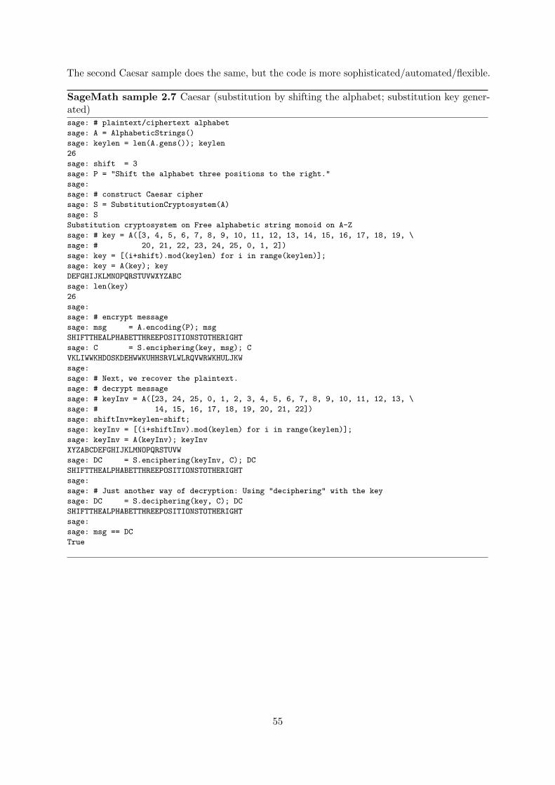
The second Caesar sample does the same, but the code is more sophisticated/automated/flexible.
SageMath sample 2.7 Caesar (substitution by shifting the alphabet; substitution key gener-ated)sage: # plaintext/ciphertext alphabet
sage: A = AlphabeticStrings()
sage: keylen = len(A.gens()); keylen
26
sage: shift = 3
sage: P = "Shift the alphabet three positions to the right."
sage:
sage: # construct Caesar cipher
sage: S = SubstitutionCryptosystem(A)
sage: S
Substitution cryptosystem on Free alphabetic string monoid on A-Z
sage: # key = A([3, 4, 5, 6, 7, 8, 9, 10, 11, 12, 13, 14, 15, 16, 17, 18, 19, \
sage: # 20, 21, 22, 23, 24, 25, 0, 1, 2])
sage: key = [(i+shift).mod(keylen) for i in range(keylen)];
sage: key = A(key); key
DEFGHIJKLMNOPQRSTUVWXYZABC
sage: len(key)
26
sage:
sage: # encrypt message
sage: msg = A.encoding(P); msg
SHIFTTHEALPHABETTHREEPOSITIONSTOTHERIGHT
sage: C = S.enciphering(key, msg); C
VKLIWWKHDOSKDEHWWKUHHSRVLWLRQVWRWKHULJKW
sage:
sage: # Next, we recover the plaintext.
sage: # decrypt message
sage: # keyInv = A([23, 24, 25, 0, 1, 2, 3, 4, 5, 6, 7, 8, 9, 10, 11, 12, 13, \
sage: # 14, 15, 16, 17, 18, 19, 20, 21, 22])
sage: shiftInv=keylen-shift;
sage: keyInv = [(i+shiftInv).mod(keylen) for i in range(keylen)];
sage: keyInv = A(keyInv); keyInv
XYZABCDEFGHIJKLMNOPQRSTUVW
sage: DC = S.enciphering(keyInv, C); DC
SHIFTTHEALPHABETTHREEPOSITIONSTOTHERIGHT
sage:
sage: # Just another way of decryption: Using "deciphering" with the key
sage: DC = S.deciphering(key, C); DC
SHIFTTHEALPHABETTHREEPOSITIONSTOTHERIGHT
sage:
sage: msg == DC
True
55

2.5.2.2 Shift cipher
The shift cipher can also be thought of as a generalization of the Caesar cipher. While theCaesar cipher restricts us to shift exactly three positions along an alphabet, the shift cipherallows us to shift any number of positions along the alphabet.
In the above samples we applied the SubstitutionCryptosystem and build Caesar as aspecial kind of substitution. In contrast here Caesar can be build as a special kind of the shiftcipher.
The shift cipher is implemented directly in the SageMath class
sage.crypto.classical.ShiftCryptosystem
In the following example, we construct a shift cipher over the capital letters of the Englishalphabet. We then encrypt a plaintext P by shifting it 12 positions along the alphabet. Finally,we decrypt the ciphertext C and make sure that the result (DC) is indeed the original plaintext.Shifting is a special way of substitution.
SageMath sample 2.8 A shift cipher over the upper-case letters of the English alphabetsage: # construct Shift cipher directly
sage: shiftcipher = ShiftCryptosystem(AlphabeticStrings()); shiftcipher
Shift cryptosystem on Free alphabetic string monoid on A-Z
sage: P = shiftcipher.encoding("Shift me any number of positions."); P
SHIFTMEANYNUMBEROFPOSITIONS
sage: key = 12 # shift can be any integer number
sage:
sage: # shift the plaintext by 12 positions to get the ciphertext
sage: C = shiftcipher.enciphering(key, P); C
ETURFYQMZKZGYNQDARBAEUFUAZE
sage:
sage: # decrypt the ciphertext and ensure that it is the original plaintext
sage: DC = shiftcipher.deciphering(key, C); DC
SHIFTMEANYNUMBEROFPOSITIONS
sage: DC == P
True
The Caesar cipher is simply a shift cipher whose shifting key is 3. In the next example, weuse the shift cipher to create a Caesar cipher over the capital letters of the English alphabet.
SageMath sample 2.9 Constructing the Caesar cipher using the shift ciphersage: # create a Caesar cipher
sage: caesarcipher = ShiftCryptosystem(AlphabeticStrings())
sage: P = caesarcipher.encoding("Shift the alphabet by three positions to the right."); P
SHIFTTHEALPHABETBYTHREEPOSITIONSTOTHERIGHT
sage:
sage: key = 3 # shift the plaintext by exactly 3 positions
sage: C = caesarcipher.enciphering(key, P); C
VKLIWWKHDOSKDEHWEBWKUHHSRVLWLRQVWRWKHULJKW
sage:
sage: # decrypt the ciphertext and ensure that it is the original plaintext
sage: DC = caesarcipher.deciphering(key, C); DC
SHIFTTHEALPHABETBYTHREEPOSITIONSTOTHERIGHT
sage: DC == P
True
56

2.5.2.3 Affine cipher
The affine cipher is implemented in the SageMath class
sage.crypto.classical.AffineCryptosystem
In the following example, we construct an affine cipher ci = b ∗ pi + a with key (3, 13) anduse this key to encrypt a given plaintext P = (p1, p2, ..., pn). The plaintext is then decryptedand the result DC is compared to the original plaintext.
SageMath sample 2.10 An affine cipher with key (3, 13)sage: # create an affine cipher
sage: affineCipher = AffineCryptosystem(AlphabeticStrings()); affineCipher
Affine cryptosystem on Free alphabetic string monoid on A-Z
sage: P = affineCipher.encoding("The affine cryptosystem.")
sage: P
THEAFFINECRYPTOSYSTEM
sage:
sage: # encrypt the plaintext using the key (3, 13)
sage: a, b = (3, 13)
sage: C = affineCipher.enciphering(a, b, P)
sage: C
SIZNCCLAZTMHGSDPHPSZX
sage:
sage: # decrypt the ciphertext and make sure that it is equivalent to the original plaintext
sage: DC = affineCipher.deciphering(a, b, C)
sage: DC
THEAFFINECRYPTOSYSTEM
sage: DC == P
True
We can also construct a shift cipher using the affine cipher. To do so, we need to restrictkeys of the affine cipher be of the form (1, b) where b is any non-negative integer. For instance,we can work through SageMath example 2.8 on page 56 as follows:
SageMath sample 2.11 Constructing a shift cipher using the affine ciphersage: # construct a shift cipher
sage: shiftcipher = AffineCryptosystem(AlphabeticStrings()); shiftcipher
Affine cryptosystem on Free alphabetic string monoid on A-Z
sage: P = shiftcipher.encoding("Shift me any number of positions.")
sage: P
SHIFTMEANYNUMBEROFPOSITIONS
sage:
sage: # shift the plaintext by 12 positions to get the ciphertext
sage: a, b = (1, 12)
sage: C = shiftcipher.enciphering(a, b, P)
sage: C
ETURFYQMZKZGYNQDARBAEUFUAZE
sage:
sage: # decrypt the ciphertext and ensure that it is the original plaintext
sage: DC = shiftcipher.deciphering(a, b, C); P
SHIFTMEANYNUMBEROFPOSITIONS
sage: DC == P
True
We can also use the affine cipher to create the Caesar cipher. To do so, the encryp-
57
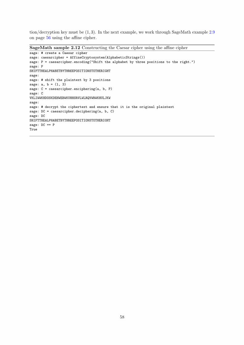
tion/decryption key must be (1, 3). In the next example, we work through SageMath example 2.9on page 56 using the affine cipher.
SageMath sample 2.12 Constructing the Caesar cipher using the affine ciphersage: # create a Caesar cipher
sage: caesarcipher = AffineCryptosystem(AlphabeticStrings())
sage: P = caesarcipher.encoding("Shift the alphabet by three positions to the right.")
sage: P
SHIFTTHEALPHABETBYTHREEPOSITIONSTOTHERIGHT
sage:
sage: # shift the plaintext by 3 positions
sage: a, b = (1, 3)
sage: C = caesarcipher.enciphering(a, b, P)
sage: C
VKLIWWKHDOSKDEHWEBWKUHHSRVLWLRQVWRWKHULJKW
sage:
sage: # decrypt the ciphertext and ensure that it is the original plaintext
sage: DC = caesarcipher.deciphering(a, b, C)
sage: DC
SHIFTTHEALPHABETBYTHREEPOSITIONSTOTHERIGHT
sage: DC == P
True
58

2.5.2.4 Substitution with symbols
In the following SageMath example the symbols are from the binary number system. Amonoalphabetic substitution cipher with a binary alphabet has very little security: Becausethe plaintext/ciphertext alphabet has only the two elements 0 and 1, there are only two keyspossible: (0 1) and (1 0).Remark: The key of a general substitution cipher contains all symbols of the alphabet exactlyonce.
SageMath sample 2.13 Monoalphabetic substitution with a binary alphabetsage: # the plaintext/ciphertext alphabet
sage: B = BinaryStrings()
sage: # substitution cipher over the alphabet B; no keylen argument possible
sage: S = SubstitutionCryptosystem(B); S
Substitution cryptosystem on Free binary string monoid
sage: # To get a substitute for each symbol, key has always the length of the alphabet
sage: key = S.random_key(); key
10
sage: len(key)
2
sage: P = "Working with binary numbers."
sage: # encryption
sage: msg = B.encoding(P); msg
01010111011011110111001001101011011010010110111001100111001000000111011101101\
00101110100011010000010000001100010011010010110111001100001011100100111100100\
1000000110111001110101011011010110001001100101011100100111001100101110
sage: C = S.enciphering(key, msg); C
10101000100100001000110110010100100101101001000110011000110111111000100010010\
11010001011100101111101111110011101100101101001000110011110100011011000011011\
0111111001000110001010100100101001110110011010100011011000110011010001
sage: # decryption
sage: DC = S.deciphering(key, C); DC
01010111011011110111001001101011011010010110111001100111001000000111011101101\
00101110100011010000010000001100010011010010110111001100001011100100111100100\
1000000110111001110101011011010110001001100101011100100111001100101110
sage: msg == DC
True
Remark: Currently S has no attribute key, and I found no way to transform the binarysequence DC back to ASCII.
59

The second sample of a monoalphabetic substitution with symbols uses a larger alphabet asplaintext/ciphertext space as the first sample. Here the hexadecimal number system is used assubstitution alphabet.
SageMath sample 2.14 Monoalphabetic substitution with a hexadecimal alphabet (anddecoding in Python)sage: A = HexadecimalStrings()
sage: S = SubstitutionCryptosystem(A)
sage: key = S.random_key(); key
2b56a4e701c98df3
sage: len(key)
16
sage: # Number of possible keys
sage: factorial(len(key))
20922789888000
sage: P = "Working with a larger alphabet."
sage:
sage: msg = A.encoding(P); msg
576f726b696e6720776974682061206c617267657220616c7068616265742e
sage: C = S.enciphering(key, msg); C
47e375e9e1efe75277e17ae052eb52e8eb75e7e47552ebe872e0ebe5e47a5f
sage: DC = S.deciphering(key, C); DC
576f726b696e6720776974682061206c617267657220616c7068616265742e
sage: msg == DC
True
sage:
sage: # Conversion hex back to ASCII:
sage: # - AlphabeticStrings() and HexadecimalStrings() don’t have according methods.
sage: # - So we used Python directly.
sage: import binascii
sage: DDC = binascii.a2b_hex(repr(DC)); DDC
’Working with a larger alphabet.’
sage:
sage: P == DDC
True
60

2.5.2.5 Vigenere cipher
The Vigenere cipher is implemented in the SageMath class
sage.crypto.classical.VigenereCryptosystem
For our ciphertext/plaintext space, we can work with the upper-case letters of the Englishalphabet, the binary number system, the octal number system, or the hexadecimal numbersystem. Here is an example using the class AlphabeticStrings, which implements the Englishcapital letters.
SageMath sample 2.15 Vigenere ciphersage: # construct Vigenere cipher
sage: keylen = 14
sage: A = AlphabeticStrings()
sage: V = VigenereCryptosystem(A, keylen); V
Vigenere cryptosystem on Free alphabetic string monoid on A-Z of period 14
sage:
sage: # alternative could be a given key: key = A(’ABCDEFGHIJKLMN’); key
sage: key = V.random_key(); key
WSSSEEGVVAARUD
sage: len(key)
14
sage:
sage: # encoding
sage: P = "The Vigenere cipher is polyalphabetic."
sage: len(P)
38
sage: msg = V.encoding(P); msg # alternative: msg = A.encoding(P); msg
THEVIGENERECIPHERISPOLYALPHABETIC
sage:
sage: # encryption [2 alternative ways (in two steps or in one): both work]
sage: # encrypt = V(key); encrypt
sage: # C = encrypt(msg); C
sage: C = V.enciphering(key, msg); C
PZWNMKKIZRETCSDWJAWTUGTALGBDXWLAG
sage:
sage: # decryption
sage: DC = V.deciphering(key, C); DC
THEVIGENERECIPHERISPOLYALPHABETIC
sage: msg == DC
True
61
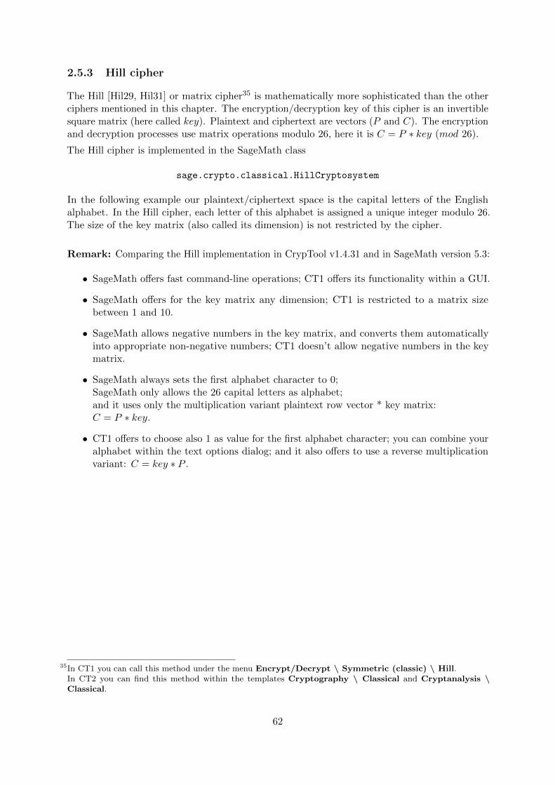
2.5.3 Hill cipher
The Hill [Hil29, Hil31] or matrix cipher35 is mathematically more sophisticated than the otherciphers mentioned in this chapter. The encryption/decryption key of this cipher is an invertiblesquare matrix (here called key). Plaintext and ciphertext are vectors (P and C). The encryptionand decryption processes use matrix operations modulo 26, here it is C = P ∗ key (mod 26).
The Hill cipher is implemented in the SageMath class
sage.crypto.classical.HillCryptosystem
In the following example our plaintext/ciphertext space is the capital letters of the Englishalphabet. In the Hill cipher, each letter of this alphabet is assigned a unique integer modulo 26.The size of the key matrix (also called its dimension) is not restricted by the cipher.
Remark: Comparing the Hill implementation in CrypTool v1.4.31 and in SageMath version 5.3:
• SageMath offers fast command-line operations; CT1 offers its functionality within a GUI.
• SageMath offers for the key matrix any dimension; CT1 is restricted to a matrix sizebetween 1 and 10.
• SageMath allows negative numbers in the key matrix, and converts them automaticallyinto appropriate non-negative numbers; CT1 doesn’t allow negative numbers in the keymatrix.
• SageMath always sets the first alphabet character to 0;SageMath only allows the 26 capital letters as alphabet;and it uses only the multiplication variant plaintext row vector * key matrix:C = P ∗ key.
• CT1 offers to choose also 1 as value for the first alphabet character; you can combine youralphabet within the text options dialog; and it also offers to use a reverse multiplicationvariant: C = key ∗ P .
35In CT1 you can call this method under the menu Encrypt/Decrypt \ Symmetric (classic) \ Hill.In CT2 you can find this method within the templates Cryptography \ Classical and Cryptanalysis \Classical.
62

SageMath sample 2.16 Hill cipher with randomly generated key matrixsage: # construct a Hill cipher
sage: keylen = 19 # An Alternative could be: Use a non-random small key (e.g. keylen = 3)
sage: A = AlphabeticStrings(); H = HillCryptosystem(A, keylen); H
Hill cryptosystem on Free alphabetic string monoid on A-Z of block length 19
sage:
sage: # Alternative: Here, HKS is necessary in addition [H.key_space() isn’t enough].
sage: # HKS = H.key_space(); key = HKS([[1,0,1],[0,1,1],[2,2,3]]); key
sage:
sage: # Random key creation
sage: key = H.random_key(); key
[10 7 5 2 0 6 10 23 15 7 17 19 18 2 9 12 0 10 11]
[23 1 1 10 4 9 21 1 25 22 19 8 17 22 15 8 12 25 22]
[ 4 12 16 15 1 12 24 5 9 13 5 15 8 21 23 24 22 20 6]
[ 5 11 6 7 3 12 8 9 21 20 9 4 16 18 10 3 2 23 18]
[ 8 22 14 14 20 13 21 19 3 13 2 11 13 23 9 25 25 6 8]
[24 25 8 24 7 18 3 20 6 11 25 5 6 19 7 24 2 4 10]
[15 25 11 1 4 7 11 24 20 2 18 4 9 8 12 19 24 0 12]
[14 6 2 9 11 20 13 4 10 11 4 23 14 22 14 16 9 12 18]
[12 10 21 5 21 15 16 17 19 20 1 1 15 5 0 2 23 4 14]
[21 15 15 16 15 20 4 10 25 7 15 4 7 12 24 9 19 10 6]
[25 15 2 3 17 23 21 16 8 18 23 4 22 11 15 19 6 0 15]
[14 23 9 3 18 15 10 18 7 5 12 23 11 9 22 21 20 4 14]
[ 3 6 8 13 20 16 11 1 13 10 4 21 25 15 12 3 0 11 18]
[21 25 14 6 11 3 21 0 19 17 5 8 5 4 9 2 23 19 15]
[ 8 11 9 11 20 15 6 1 3 18 18 22 16 17 6 3 15 11 2]
[21 15 5 22 2 9 0 4 22 10 2 10 19 19 17 19 1 21 4]
[ 7 17 9 2 15 5 14 3 6 9 12 12 22 15 8 4 21 14 19]
[19 14 24 19 7 5 22 22 13 14 7 18 17 19 25 2 1 23 6]
[ 2 6 14 22 17 7 23 6 22 7 13 20 0 14 23 17 6 1 12]
sage:
sage: # encoding and encryption
sage: P = "Hill or matrix cipher uses matrix operations."; len(P)
45
sage: # implementation requires: Length of msg is a multiple of matrix dimension (block_length)
sage: msg = H.encoding(P); msg; len(msg)
HILLORMATRIXCIPHERUSESMATRIXOPERATIONS
38
sage:
sage: # encryption (the length of msg must be a multiple of keylen).
sage: C = H.enciphering(key, msg); C
CRWCKPRVYXNBRZTNZCTQWFWSDWBCHABGMNEHVP
sage:
sage: # decryption
sage: DC = H.deciphering(key, C); DC; msg == DC
HILLORMATRIXCIPHERUSESMATRIXOPERATIONS
True
sage:
sage: # alternative decryption using inverse matrix
sage: keyInv = H.inverse_key(key); keyInv
[ 6 23 1 23 3 12 17 22 6 16 22 14 18 3 1 10 21 16 20]
[18 23 15 25 24 23 7 4 10 7 21 7 9 0 13 22 5 5 23]
...
[10 11 12 6 11 17 13 9 19 16 14 24 4 8 5 16 18 20 1]
[19 16 16 21 1 19 7 12 3 18 1 17 7 10 24 21 7 16 11]
sage: DC = H.enciphering(keyInv, C); DC
HILLORMATRIXCIPHERUSESMATRIXOPERATIONS
63
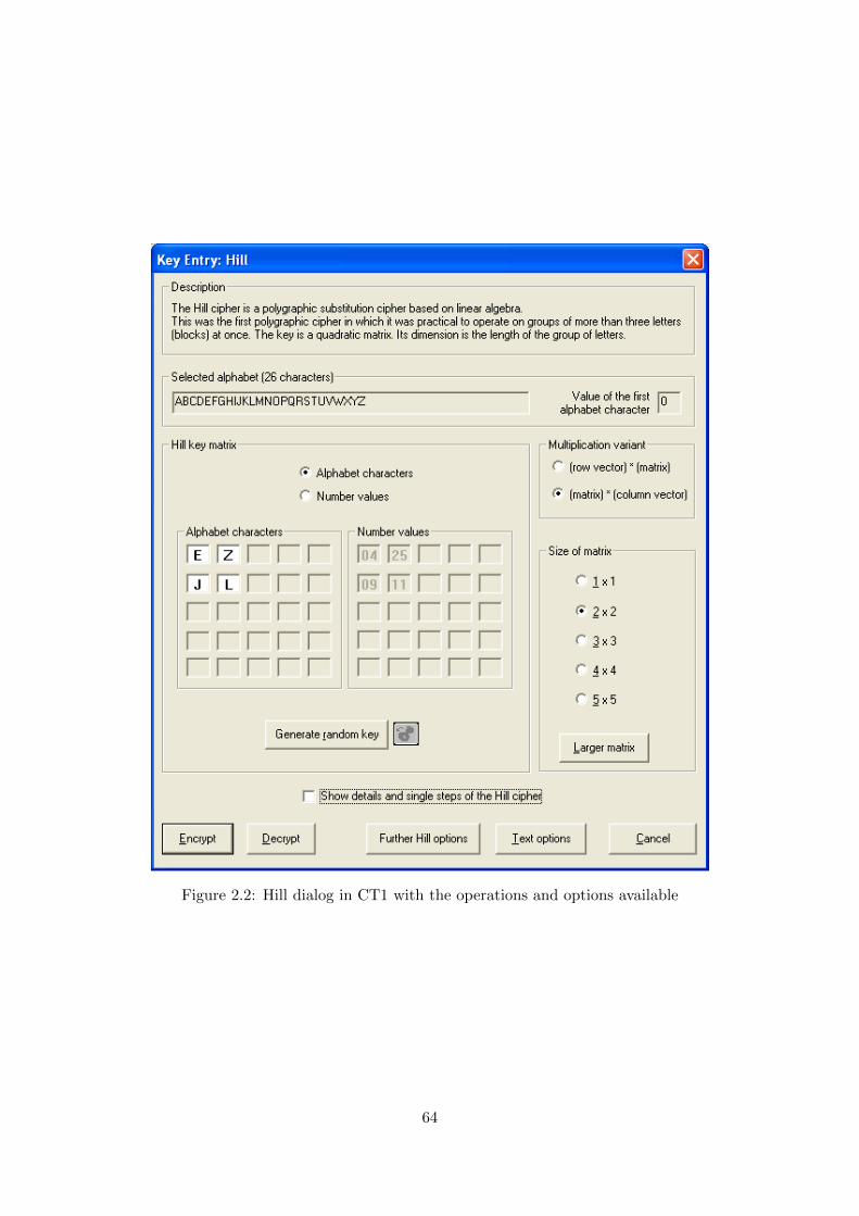
Figure 2.2: Hill dialog in CT1 with the operations and options available
64

Bibliography (Chap PaP)
[ACA02] ACA: Length and Standards for all ACA Ciphers. Technical report, American Cryp-togram Association, 2002.http://www.cryptogram.org/cdb/aca.info/aca.and.you/chap08.html#,http://www.und.edu/org/crypto/crypto/.chap08.html.
[Cro00] Crowley, Paul: Mirdek: A card cipher inspired by “Solitaire”, 2000. http://www.ciphergoth.org/crypto/mirdek/.
[Dro15] Drobick, Jorg: Abriss DDR-Chiffriergeschichte: SAS- und Chiffrierdienst, 2015. http://scz.bplaced.net/m.html#dwa.
[Goe14] Goebel, Greg: Codes, Ciphers and Codebreaking, 2014. Version 2.3.2. http://www.vectorsite.net/ttcode.html.
[Hil29] Hill, Lester S.: Cryptography in an Algebraic Alphabet. The American MathematicalMonthly, 36(6):306–312, 1929.
[Hil31] Hill, Lester S.: Concerning Certain Linear Transformation Apparatus of Cryptography.The American Mathematical Monthly, 38(3):135–154, 1931.
[Ngu09] Nguyen, Minh Van: Exploring Cryptography Using the Sage Computer Algebra System.Master’s thesis, Victoria University, 2009.http://www.sagemath.org/files/thesis/nguyen-thesis-2009.pdf,http://www.sagemath.org/library-publications.html.
[Sav99] Savard, John J. G.: A Cryptographic Compendium, 1999.http://www.quadibloc.com/crypto/jscrypt.htm.
[Sch99] Schneier, Bruce: The Solitaire Encryption Algorithm, 1999. v. 1.2.https://www.schneier.com/academic/solitaire/.
[Sin99] Singh, Simon: The Code Book: The Science of Secrecy from Ancient Egypt to QuantumCryptography. Anchor, 1999.
[Thi99] ThinkQuest Team 27158: Data Encryption, 1999.
[WLS99] Witten, Helmut, Irmgard Letzner, and Ralph Hardo Schulz: RSA & Co. in der Schule:Moderne Kryptologie, alte Mathematik, raffinierte Protokolle. Teil 3: Flusschiffren,perfekte Sicherheit und Zufall per Computer. LOG IN, 1999(2):50–57, 1999. http:
//bscw.schule.de/pub/nj_bscw.cgi/d637156/RSA_u_Co_T3.pdf.
All links have been confirmed at July 11, 2016.
65

Chapter 3
Prime Numbers
(Bernhard Esslinger, May 1999; Updates: Nov 2000, Dec 2001, Jun 2003, May 2005, Mar 2006,Jun 2007, Jan 2010, Aug 2013, Jul 2016, Apr 2018)
Progress requires exchange of knowledge.
Quote 6: Albert Einstein1
3.1 What are prime numbers?
Prime numbers are whole, positive numbers greater than or equal to 2 that can only be divided by1 and themselves. All other natural numbers greater than or equal to 4 are composite numbers,and can be formed by multiplying prime numbers.
The natural numbers N = {1, 2, 3, 4, · · · } thus comprise
• the number 1 (the unit value)
• the primes and
• the composite numbers.
Prime numbers are particularly important for three reasons:
• In number theory, they are considered to be the basic components of natural numbers,upon which numerous brilliant mathematical ideas are based.
• They are of extreme practical importance in modern cryptography (public key cryptog-raphy). The most common public key procedure, invented at the end of the 1970’s, isRSA encryption. Only using (large) prime numbers for particular parameters can youguarantee that an algorithm is secure, both for the RSA procedure and for even moremodern procedures (e.g. elliptic curves).
• The search for the largest known prime numbers does not have any practical usage known todate, but requires the best computers, is an excellent benchmark (possibility for determiningthe performance of computers) and leads to new calculation methods on many computers(see also: http://www.mersenne.org/prime.htm).
1Albert Einstein, German physicist and Nobel Prize winner, Mar 14, 1879 − Apr 14, 1955.
66
Many people have been fascinated by prime numbers over the past two millennia. Ambitionto make new discoveries about prime numbers has often resulted in brilliant ideas and conclusions.The following section provides an easily comprehensible introduction to the basics of primenumbers. We will also explain what is known about the distribution (density, number of primenumbers in particular intervals) of prime numbers and how prime number tests work.
3.2 Prime numbers in mathematics
Every whole number has a factor. The number 1 only has one factor, itself, whereas the number12 has the six factors 1, 2, 3, 4, 6, 12. Many numbers can only be divided by themselves and by 1.With respect to multiplication, these are the “atoms” in the area of numbers. Such numbers arecalled prime numbers.
In mathematics, a slightly different (but equivalent) definition is used.
Definition 3.2.1. A whole number p ∈ N is called prime if p > 1 and p only possesses thetrivial factors ±1 and ±p.
By definition, the number 1 is not a prime number. In the following sections, p will alwaysdenote a prime number.
The sequence of prime numbers starts with
2, 3, 5, 7, 11, 13, 17, 19, 23, 29, 31, 37, 41, 43, 47, 53, 59, 61, 67, 71, 73, 79, 83, 89, 97, · · · .
The first 100 numbers include precisely 25 prime numbers. After this, the percentage of primesconstantly decreases. Prime numbers can be factorized in a uniquely trivial way:
5 = 1 · 5, 17 = 1 · 17, 1013 = 1 · 1013, 1, 296, 409 = 1 · 1, 296, 409.
All numbers that have 2 or more factors not equal 1 are called composite numbers. These include
4 = 2 · 2, 6 = 2 · 3
as well as numbers that look like primes, but are in fact composite:
91 = 7 · 13, 161 = 7 · 23, 767 = 13 · 59.
67

The following table gives a first impression how primes are distributed between naturalnumbers. There are many graphical forms of represenation (the most well-known is the Ulamspiral). However till now, these graphical forms gained no new insights, but for some people theycreated the impression that there are at least local patterns within the random distribution.
Figure 3.1: Primes within the first 390 integers – marked with color2
Figure 3.2: Primes within the first 999 integers – as Ulam spiral3
Figure 3.3: Primes within the first 4000 integers – as Ulam spiral4
2Graphics from http://mathforum.org/mathimages/index.php/Image:Irisprime.jpg, 30*13 rectangle3Graphics from CT2, menu Crypto Tutorials, World of Primes, Distribution of primes, Ulam’s spiral; 32*32 points.
68

Theorem 3.2.1. Each whole number m greater than 1 possesses a lowest factor greater than 1.This is a prime number p. Unless m is a prime number itself, then: p is less than or equal to thesquare root of m.
All whole numbers greater than 1 can be expressed as a product of prime numbers — ina unique way. This is the claim of the 1st fundamental theorem of number theory (=fundamental theorem of arithmetic = fundamental building block of all positive integers).
Theorem 3.2.2. Each element n of the natural numbers greater than 1 can be written as theproduct n = p1 · p2 . . . pm of prime numbers. If two such factorizations
n = p1 · p2 · · · · · pm = p′1 · p′2 · · · p′m′
are given, then they can be reordered such that m = m′ and for all i: pi = p′i.(p1, p2, . . . , pm are called the prime factors of n).
In other words: each natural number other than 1 can be written as a product of primenumbers in precisely one way, if we ignore the order of the factors. The factors are thereforeunique (the expression as a product of factors is unique)! For example,
60 = 2 · 2 · 3 · 5 = 22 · 31 · 51.
And this — other than changing the order of the factors — is the only way in which the number60 can be factorized. If you allow numbers other than primes as factors, there are several waysof factorizing integers and the uniqueness is lost:
60 = 1 · 60 = 2 · 30 = 4 · 15 = 5 · 12 = 6 · 10 = 2 · 3 · 10 = 2 · 5 · 6 = 3 · 4 · 5 = · · · .
The following section is aimed more at those familiar with mathematical logic: The 1stfundamental theorem only appears to be obvious . We can construct numerous other sets ofnumbers (i.e. other than positive whole numbers greater than 1), for which numbers in theset cannot be expressed uniquely as a product of the prime numbers of the set: In the setM = {1, 5, 10, 15, 20, · · · } there is no equivalent to the fundamental theorem under multiplication.The first five prime numbers of this sequence are 5, 10, 15, 20, 30 (note: 10 is prime, because 5 isnot a factor of 10 in this set — the result is not an element of the given basic set M). Becausethe following applies in M :
100 = 5 · 20 = 10 · 10
and 5, 10, 20 are all prime numbers in this set, the expression as a product of prime factors isnot unique here.
3.3 How many prime numbers are there?
For the natural numbers, the primes can be compared to elements in chemistry or the elementaryparticles in physics (see [Blu99, p. 22]).
Although there are only 92 natural chemical elements, the number of prime numbers isunlimited. Even the Greek, Euclid5 knew this in the third century B.C.
4Graphics from http://mathforum.org/mathimages/index.php/Image:Ulam_spiral.png, 200*200 Ulam spiral5Euclid, a Greek mathematician of 4th and 3rd century B.C. He worked at the Egyptian academy of Alexandriaand wrote “The Elements”, the most well known systematically textbook of the Greek mathematics.
69

Theorem 3.3.1 (Euclid6). The sequence of prime numbers does not discontinue. Therefore, thequantity of prime numbers is infinite.
His proof that there is an infinite number of primes is still considered to be a brilliantmathematical consideration and conclusion today (proof by contradiction ). He assumedthat there is only a finite number of primes and therefore a largest prime number. Based on thisassumption, he drew logical conclusions until he obtained an obvious contradiction. This meantthat something must be wrong. As there were no mistakes in the chain of conclusions, it couldonly be the assumption that was wrong. Therefore, there must be an infinite number of primes!
Proof according to Euclid (proof by contradiction)
Assumption: There is a finite number of primes.
Conclusion: Then these can be listed p1 < p2 < p3 < · · · < pn, where n is the (finite)number of prime numbers. pn is therefore the largest prime. Euclid now looks at the numbera = p1 · p2 · · · pn + 1. This number cannot be a prime number because it is not included inour list of primes. It must therefore be divisible by a prime, i.e. there is a natural number ibetween 1 and n, such that pi divides the number a. Of course, pi also divides the producta− 1 = p1 · p2 · · · pn, because pi is a factor of a− 1. Since pi divides the numbers a and a− 1, italso divides the difference of these numbers. Thus: pi divides a− (a− 1) = 1. pi must thereforedivide 1, which is impossible.
Contradiction: Our assumption was false.
Thus there is an infinite number of primes (Cross-reference: overview under 3.9 of the numberof prime numbers in various intervals). 2
Here we should perhaps mention yet another fact which is initially somewhat surprising.Namely, in the prime numbers sequence p1, p2, · · · , gaps between prime numbers can have anindividually determined length n. It is undeniable that under the n succession of natural numbers
(n+ 1)! + 2, · · · , (n+ 1)! + (n+ 1),
none of them is a prime number since in order, the numbers 2, 3, · · · , (n + 1) are comprisedrespectively as real divisors. (n! means the product of the first n natural numbers thereforen! = n ∗ (n− 1) ∗ · · · ∗ 2 ∗ 1).
6The common usage of the term does not denote Euclid as the inventor of the theorem rather; the true inventor ismerely not as prominent. The theorem has already been distinguished and proven in Euclid’s Elements (Book IX,theorem 20). The phraseology is remarkable due to the fact that the word infinite is not used. The text reads asfollowed
Oι π%ωτoι α%ιϑµoι πλειoυς εισι παντ oς τoυ π%oτεϑεντoς πληϑ oυς π%ωτων α%ιϑµων,
the English translation of which is: the prime numbers are more than any previously existing amount of primenumbers.
70
3.4 The search for extremely large primes
The largest prime numbers known today have several millions digits.7 This is too big for us toimagine. The number of elementary particles in the universe is estimated to be “only” a 80-digitdecimal number (see the overview under 3.11 of various orders of magnitude / dimensions).
3.4.1 The 30+ largest known primes (as of Jan 2018)
The following table 3.1 contains the biggest, currently known primes and a description of itsparticular number type.8
7In CT1 you can calculate all digits of such a big number very quickly via the menu path Indiv. Procedures \Number Theory Interactive \ Compute Mersenne Numbers.
8An up-to-date version can be found in the internet at https://primes.utm.edu/primes/search.php?Number=1000,at http://primes.utm.edu/mersenne/index.html, and at http://www.mersenne.org/primes/.
9This number was found within the distributed computing project “Seventeen or Bust” (SoB) (https://en.wikipedia.org/wiki/Seventeen_or_Bust) at March 26, 2007. While the well known GIMPS project (chapter 3.4.2)searches for bigger and bigger of the infinitely many primes, there is a chance, that the SoB project could havebeen completed its task sometime.
The SoB project tries to prove computationally, that the number k = 78, 557 is the smallest Sierpinski number(John Selfridge proved in 1962, that 78, 557 is a Sierpinski number).
The famous Polish mathematician Waclaw Sierpinski (1882 to 1969) proved in 1960, that there exist infinitelymany odd integers k, which fulfill the following property: For all Sierpinski numbers k it is true: All numbersN = k · 2n + 1 are composite for all integers n >= 1 (Sierpinski’s Composite Number Theorem, http://mathworld.wolfram.com/SierpinskisCompositeNumberTheorem.html).
When the project started in 2002 there have been 17 possible candidates < 78557 (this is the reason for theproject’s name “Seventeen or Bust”). It is sufficient to find one single counter-example, to exclude a candidate k,which means to find a single n >= 1, where N = k · 2n + 1 is prime. So it is only a byproduct of this task thatthis also generates new monster primes.
As of about April 19, 2016, the main SoB server is down and the future of the project unknown.10Generalized Fermat number: 1, 372, 930131,072 + 1 = 1, 372, 930(217) + 1
71
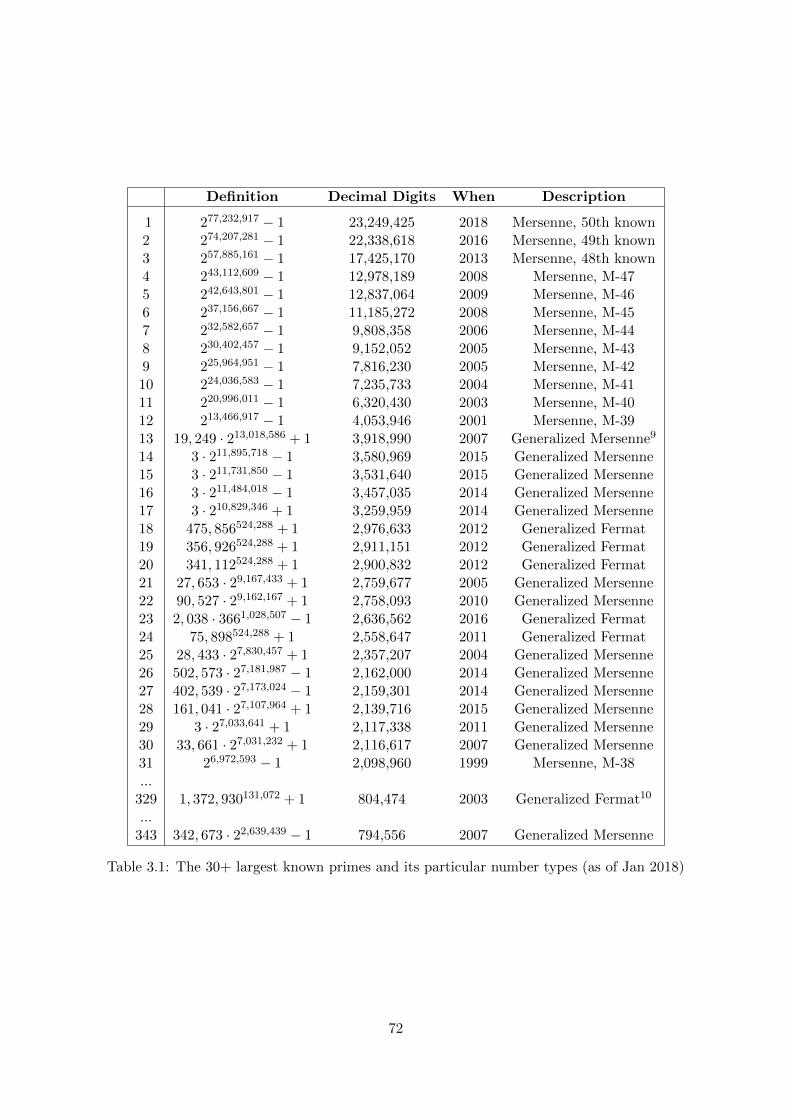
Definition Decimal Digits When Description
1 277,232,917 − 1 23,249,425 2018 Mersenne, 50th known2 274,207,281 − 1 22,338,618 2016 Mersenne, 49th known3 257,885,161 − 1 17,425,170 2013 Mersenne, 48th known4 243,112,609 − 1 12,978,189 2008 Mersenne, M-475 242,643,801 − 1 12,837,064 2009 Mersenne, M-466 237,156,667 − 1 11,185,272 2008 Mersenne, M-457 232,582,657 − 1 9,808,358 2006 Mersenne, M-448 230,402,457 − 1 9,152,052 2005 Mersenne, M-439 225,964,951 − 1 7,816,230 2005 Mersenne, M-4210 224,036,583 − 1 7,235,733 2004 Mersenne, M-4111 220,996,011 − 1 6,320,430 2003 Mersenne, M-4012 213,466,917 − 1 4,053,946 2001 Mersenne, M-3913 19, 249 · 213,018,586 + 1 3,918,990 2007 Generalized Mersenne9
14 3 · 211,895,718 − 1 3,580,969 2015 Generalized Mersenne15 3 · 211,731,850 − 1 3,531,640 2015 Generalized Mersenne16 3 · 211,484,018 − 1 3,457,035 2014 Generalized Mersenne17 3 · 210,829,346 + 1 3,259,959 2014 Generalized Mersenne18 475, 856524,288 + 1 2,976,633 2012 Generalized Fermat19 356, 926524,288 + 1 2,911,151 2012 Generalized Fermat20 341, 112524,288 + 1 2,900,832 2012 Generalized Fermat21 27, 653 · 29,167,433 + 1 2,759,677 2005 Generalized Mersenne22 90, 527 · 29,162,167 + 1 2,758,093 2010 Generalized Mersenne23 2, 038 · 3661,028,507 − 1 2,636,562 2016 Generalized Fermat24 75, 898524,288 + 1 2,558,647 2011 Generalized Fermat25 28, 433 · 27,830,457 + 1 2,357,207 2004 Generalized Mersenne26 502, 573 · 27,181,987 − 1 2,162,000 2014 Generalized Mersenne27 402, 539 · 27,173,024 − 1 2,159,301 2014 Generalized Mersenne28 161, 041 · 27,107,964 + 1 2,139,716 2015 Generalized Mersenne29 3 · 27,033,641 + 1 2,117,338 2011 Generalized Mersenne30 33, 661 · 27,031,232 + 1 2,116,617 2007 Generalized Mersenne31 26,972,593 − 1 2,098,960 1999 Mersenne, M-38...
329 1, 372, 930131,072 + 1 804,474 2003 Generalized Fermat10
...343 342, 673 · 22,639,439 − 1 794,556 2007 Generalized Mersenne
Table 3.1: The 30+ largest known primes and its particular number types (as of Jan 2018)
72

The development over time is shown in figure 3.4. It starts with M21701 found in 1978. Notethe vertical scale.
Figure 3.4: Number of digits of largest known prime by year (as of July 2016)11
The largest currently known prime is a Mersenne prime, found by the GIMPS project(chapter 3.4.2). Within the largest known primes there are also numbers of the type generalizedMersenne number (chapter 3.6.2) and generalized Fermat numbers (chapter 3.6.5).
11Source: Chris Caldwell, http://primes.utm.edu/notes/by_year.html
73
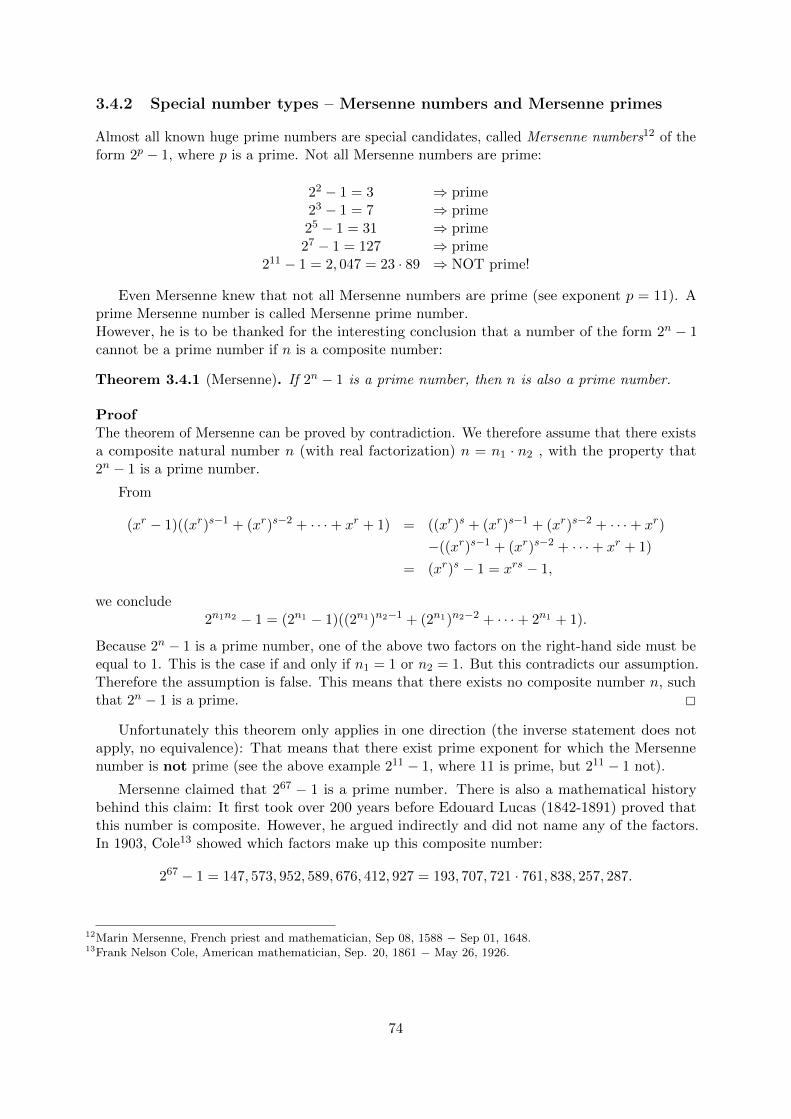
3.4.2 Special number types – Mersenne numbers and Mersenne primes
Almost all known huge prime numbers are special candidates, called Mersenne numbers12 of theform 2p − 1, where p is a prime. Not all Mersenne numbers are prime:
22 − 1 = 3 ⇒ prime23 − 1 = 7 ⇒ prime25 − 1 = 31 ⇒ prime27 − 1 = 127 ⇒ prime
211 − 1 = 2, 047 = 23 · 89 ⇒ NOT prime!
Even Mersenne knew that not all Mersenne numbers are prime (see exponent p = 11). Aprime Mersenne number is called Mersenne prime number.However, he is to be thanked for the interesting conclusion that a number of the form 2n − 1cannot be a prime number if n is a composite number:
Theorem 3.4.1 (Mersenne). If 2n − 1 is a prime number, then n is also a prime number.
ProofThe theorem of Mersenne can be proved by contradiction. We therefore assume that there existsa composite natural number n (with real factorization) n = n1 · n2 , with the property that2n − 1 is a prime number.
From
(xr − 1)((xr)s−1 + (xr)s−2 + · · ·+ xr + 1) = ((xr)s + (xr)s−1 + (xr)s−2 + · · ·+ xr)
−((xr)s−1 + (xr)s−2 + · · ·+ xr + 1)
= (xr)s − 1 = xrs − 1,
we conclude2n1n2 − 1 = (2n1 − 1)((2n1)n2−1 + (2n1)n2−2 + · · ·+ 2n1 + 1).
Because 2n − 1 is a prime number, one of the above two factors on the right-hand side must beequal to 1. This is the case if and only if n1 = 1 or n2 = 1. But this contradicts our assumption.Therefore the assumption is false. This means that there exists no composite number n, suchthat 2n − 1 is a prime. 2
Unfortunately this theorem only applies in one direction (the inverse statement does notapply, no equivalence): That means that there exist prime exponent for which the Mersennenumber is not prime (see the above example 211 − 1, where 11 is prime, but 211 − 1 not).
Mersenne claimed that 267 − 1 is a prime number. There is also a mathematical historybehind this claim: It first took over 200 years before Edouard Lucas (1842-1891) proved thatthis number is composite. However, he argued indirectly and did not name any of the factors.In 1903, Cole13 showed which factors make up this composite number:
267 − 1 = 147, 573, 952, 589, 676, 412, 927 = 193, 707, 721 · 761, 838, 257, 287.
12Marin Mersenne, French priest and mathematician, Sep 08, 1588 − Sep 01, 1648.13Frank Nelson Cole, American mathematician, Sep. 20, 1861 − May 26, 1926.
74
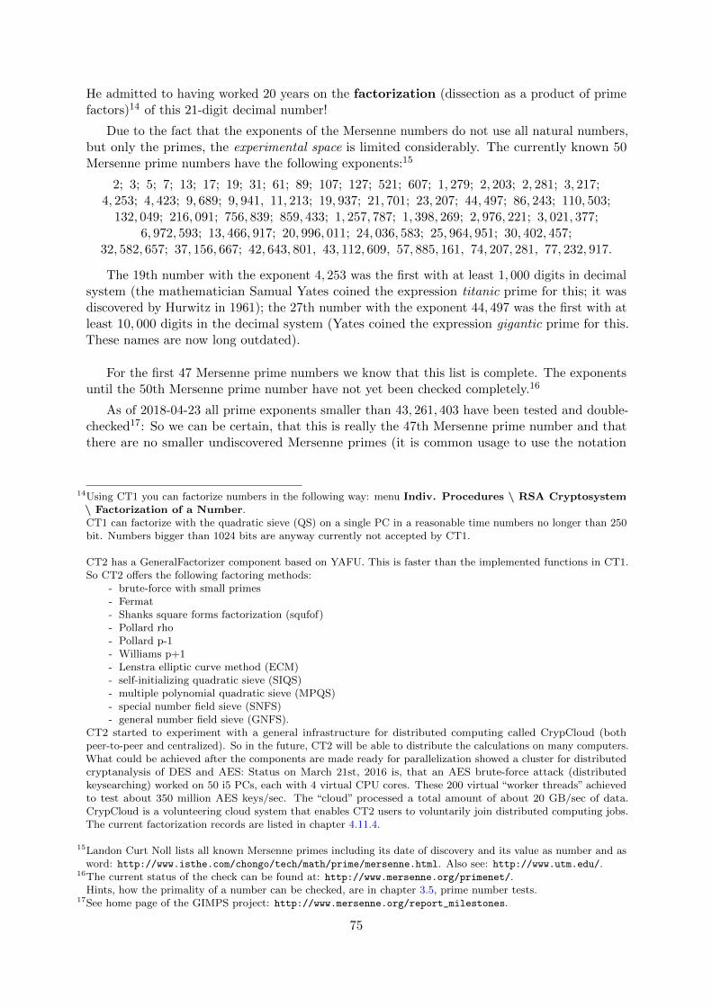
He admitted to having worked 20 years on the factorization (dissection as a product of primefactors)14 of this 21-digit decimal number!
Due to the fact that the exponents of the Mersenne numbers do not use all natural numbers,but only the primes, the experimental space is limited considerably. The currently known 50Mersenne prime numbers have the following exponents:15
2; 3; 5; 7; 13; 17; 19; 31; 61; 89; 107; 127; 521; 607; 1, 279; 2, 203; 2, 281; 3, 217;4, 253; 4, 423; 9, 689; 9, 941, 11, 213; 19, 937; 21, 701; 23, 207; 44, 497; 86, 243; 110, 503;
132, 049; 216, 091; 756, 839; 859, 433; 1, 257, 787; 1, 398, 269; 2, 976, 221; 3, 021, 377;6, 972, 593; 13, 466, 917; 20, 996, 011; 24, 036, 583; 25, 964, 951; 30, 402, 457;
32, 582, 657; 37, 156, 667; 42, 643, 801, 43, 112, 609, 57, 885, 161, 74, 207, 281, 77, 232, 917.
The 19th number with the exponent 4, 253 was the first with at least 1, 000 digits in decimalsystem (the mathematician Samual Yates coined the expression titanic prime for this; it wasdiscovered by Hurwitz in 1961); the 27th number with the exponent 44, 497 was the first with atleast 10, 000 digits in the decimal system (Yates coined the expression gigantic prime for this.These names are now long outdated).
For the first 47 Mersenne prime numbers we know that this list is complete. The exponentsuntil the 50th Mersenne prime number have not yet been checked completely.16
As of 2018-04-23 all prime exponents smaller than 43, 261, 403 have been tested and double-checked17: So we can be certain, that this is really the 47th Mersenne prime number and thatthere are no smaller undiscovered Mersenne primes (it is common usage to use the notation
14Using CT1 you can factorize numbers in the following way: menu Indiv. Procedures \ RSA Cryptosystem\ Factorization of a Number.CT1 can factorize with the quadratic sieve (QS) on a single PC in a reasonable time numbers no longer than 250bit. Numbers bigger than 1024 bits are anyway currently not accepted by CT1.
CT2 has a GeneralFactorizer component based on YAFU. This is faster than the implemented functions in CT1.So CT2 offers the following factoring methods:
- brute-force with small primes- Fermat- Shanks square forms factorization (squfof)- Pollard rho- Pollard p-1- Williams p+1- Lenstra elliptic curve method (ECM)- self-initializing quadratic sieve (SIQS)- multiple polynomial quadratic sieve (MPQS)- special number field sieve (SNFS)- general number field sieve (GNFS).
CT2 started to experiment with a general infrastructure for distributed computing called CrypCloud (bothpeer-to-peer and centralized). So in the future, CT2 will be able to distribute the calculations on many computers.What could be achieved after the components are made ready for parallelization showed a cluster for distributedcryptanalysis of DES and AES: Status on March 21st, 2016 is, that an AES brute-force attack (distributedkeysearching) worked on 50 i5 PCs, each with 4 virtual CPU cores. These 200 virtual “worker threads” achievedto test about 350 million AES keys/sec. The “cloud” processed a total amount of about 20 GB/sec of data.CrypCloud is a volunteering cloud system that enables CT2 users to voluntarily join distributed computing jobs.The current factorization records are listed in chapter 4.11.4.
15Landon Curt Noll lists all known Mersenne primes including its date of discovery and its value as number and asword: http://www.isthe.com/chongo/tech/math/prime/mersenne.html. Also see: http://www.utm.edu/.
16The current status of the check can be found at: http://www.mersenne.org/primenet/.Hints, how the primality of a number can be checked, are in chapter 3.5, prime number tests.
17See home page of the GIMPS project: http://www.mersenne.org/report_milestones.
75
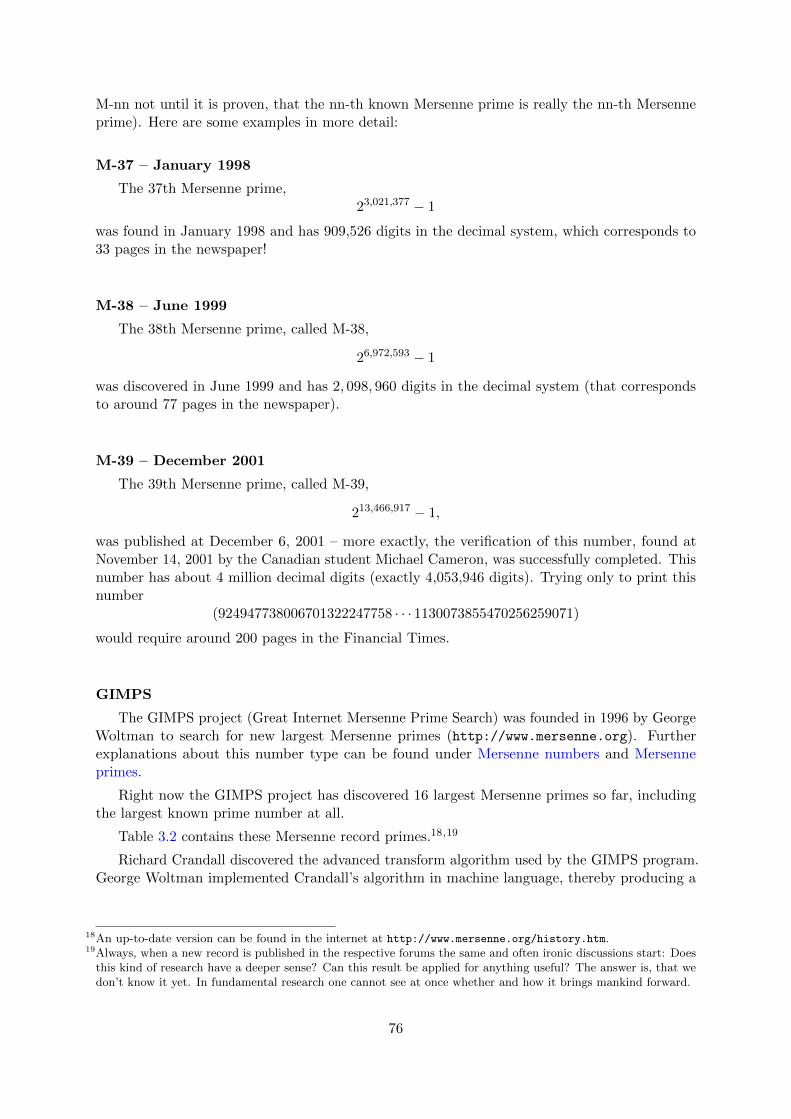
M-nn not until it is proven, that the nn-th known Mersenne prime is really the nn-th Mersenneprime). Here are some examples in more detail:
M-37 – January 1998
The 37th Mersenne prime,23,021,377 − 1
was found in January 1998 and has 909,526 digits in the decimal system, which corresponds to33 pages in the newspaper!
M-38 – June 1999
The 38th Mersenne prime, called M-38,
26,972,593 − 1
was discovered in June 1999 and has 2, 098, 960 digits in the decimal system (that correspondsto around 77 pages in the newspaper).
M-39 – December 2001
The 39th Mersenne prime, called M-39,
213,466,917 − 1,
was published at December 6, 2001 – more exactly, the verification of this number, found atNovember 14, 2001 by the Canadian student Michael Cameron, was successfully completed. Thisnumber has about 4 million decimal digits (exactly 4,053,946 digits). Trying only to print thisnumber
(924947738006701322247758 · · · 1130073855470256259071)
would require around 200 pages in the Financial Times.
GIMPS
The GIMPS project (Great Internet Mersenne Prime Search) was founded in 1996 by GeorgeWoltman to search for new largest Mersenne primes (http://www.mersenne.org). Furtherexplanations about this number type can be found under Mersenne numbers and Mersenneprimes.
Right now the GIMPS project has discovered 16 largest Mersenne primes so far, includingthe largest known prime number at all.
Table 3.2 contains these Mersenne record primes.18,19
Richard Crandall discovered the advanced transform algorithm used by the GIMPS program.George Woltman implemented Crandall’s algorithm in machine language, thereby producing a
18An up-to-date version can be found in the internet at http://www.mersenne.org/history.htm.19Always, when a new record is published in the respective forums the same and often ironic discussions start: Does
this kind of research have a deeper sense? Can this result be applied for anything useful? The answer is, that wedon’t know it yet. In fundamental research one cannot see at once whether and how it brings mankind forward.
76

Definition Decimal Digits When Who
1 277,232,917 − 1 23,249,425 Dec 26, 2017 Jonathan Pace2 274,207,281 − 1 22,338,618 Jan 7, 2016 Curtis Cooper3 257,885,161 − 1 17,425,170 Jan 25, 2013 Curtis Cooper4 243,112,609 − 1 12,978,189 Aug 23, 2008 Edson Smith5 242,643,801 − 1 12,837,064 Apr 12, 2009 Odd Magnar Strindmo6 237,156,667 − 1 11,185,272 Sep 6, 2008 Hans-Michael Elvenich7 232,582,657 − 1 9,808,358 Sep 4, 2006 Curtis Cooper/Steven Boone8 230,402,457 − 1 9,152,052 Dec 15, 2005 Curtis Cooper/Steven Boone9 225,964,951 − 1 7,816,230 Feb 18, 2005 Martin Nowak10 224,036,583 − 1 7,235,733 May 15, 2004 Josh Findley11 220,996,011 − 1 6,320,430 Nov 17, 2003 Michael Shafer12 213,466,917 − 1 4,053,946 Nov 14, 2001 Michael Cameron13 26,972,593 − 1 2,098,960 Jun 1, 1999 Nayan Hajratwala14 23,021,377 − 1 909,526 Jan 27, 1998 Roland Clarkson15 22,976,221 − 1 895,932 Aug 24, 1997 Gordon Spence16 21,398,269 − 1 420,921 November 1996 Joel Armengaud
Table 3.2: The largest primes found by the GIMPS project (as of January 2018)
prime-search program of unprecedented efficiency, and that work led to the successful GIMPSproject.
On June 1st, 2003 a possible Mersenne prime was reported to the GIMPS server, which waschecked afterwards as usual, before it was to be published. Unfortunately mid June the initiatorand GIMPS project leader George Woltman had to tell, that two independent verification runsproved the number was composite. This was the first false positive report of a client in 7 years.
Now more than 130,000 volunteers, amateurs and experts, participate in the GIMPS project.They connect their computers into the so called “PrimeNet”, originally organized by the companyEntropia from Scott Kurowski.
3.4.3 Challenge of the Electronic Frontier Foundation (EFF)
This search is also spurred on by a competition started by the non-profit organization EFF(Electronic Frontier Foundation) using the means of an unknown donor. The participants arerewarded with a total of 500,000 USD if they find the longest prime number. In promoting thisproject, the unknown donor is not looking for the quickest computer, but rather wants to drawpeople’s attention to the opportunities offered by cooperative networkinghttp://www.eff.org/awards/coop
The discoverer of M-38 received 50,000 USD from the EFF for discovering the first primewith more than 1 million decimal digits.
For the next prize of 100,000 USD offered by EFF for a proven prime with more than 10million decimal digits, Edson Smith qualified, who found the number 243,112,609 − 1 within theGIMPS project.
According to the EFF rules for their prizes they offer in the next stage 150,000 USD for aproven prime with more than 100 million decimal digits.
77

Edouard Lucas (1842-1891) held the record for the longest prime number for over 70 yearsby proving that 2127 − 1 is prime. No new record is likely to last that long.
3.5 Prime number tests20,21
In order to implement secure encryption procedures we need extremely large prime numbers(numbers in the region of 22,048 have more than 600 digits in the decimal system).
If we look for the prime factors in order to decide whether a number is prime, then thesearch takes too long, if even the smallest prime factor is enormous. Factorizing numbers usingsystematic computational division or using the sieve of Eratosthenes is only feasible using currentcomputers for numbers with up to around 20 digits in the decimal system. The biggest numberfactorized into its 2 almost equal prime factors has 232 digits (see RSA-768 in chapter 4.11.4).
However, if we know something about the construction of the number in question, there areextremely highly developed procedures that are much quicker. These procedures can determinethe primality attribute of a number, but they cannot determine the prime factors of a number,if it is compound.
In the 17th century, Fermat22 wrote to Mersenne that he presumed that all numbers of theform
f(n) = 22n
+ 1
are prime for all whole numbers n ≥ 0 (see below, chapter 3.6.4).
As early as in the 19th century, it was discovered that the 29-digit number
f(7) = 227
+ 1
is not prime. However, it was not until 1970 that Morrison/Billhart managed to factorize it.
f(7) = 340, 282, 366, 920, 938, 463, 463, 374, 607, 431, 768, 211, 457
= 59, 649, 589, 127, 497, 217 · 5, 704, 689, 200, 685, 129, 054, 721
Despite Fermat was wrong with this supposition, he is the originator of an important theoremin this area: Many rapid prime number tests are based on the (little) Fermat theorem putforward by Fermat in 1640 (see chapter 4.8.3).
Theorem 3.5.1 (“little” Fermat). Let p be a prime number and a be any whole number, thenfor all a
ap ≡ a mod p.
This could also be formulated as follows:Let p be a prime number and a be any whole number that is not a multiple of p (also a 6≡ 0 mod p),then ap−1 ≡ 1 mod p.
20A didactical article about the different prime number tests emphasizing the Miller-Rabin test can be found withinthe series RSA & Co. at school: Modern cryptology, old mathematics, and subtle protocols: see NF part 5 [WS10b].Unfortunately these are currently only available in German.
21With the educational tool for number theory NT you can apply the tests of Fermat and of Miller-Rabin: See NTlearning units 3.2 and 3.3, pages 3-11/11.NT can be called in CT1 via the menu path Indiv. Procedures \ Number Theory Interactive \ LearningTool for Number Theory. See also appendix A.6.CT2 contains a visualisation of these methods within the tutorial “World of Primes”.
22Pierre de Fermat, French mathematician, Aug 17, 1601 – Jan 12, 1665.
78
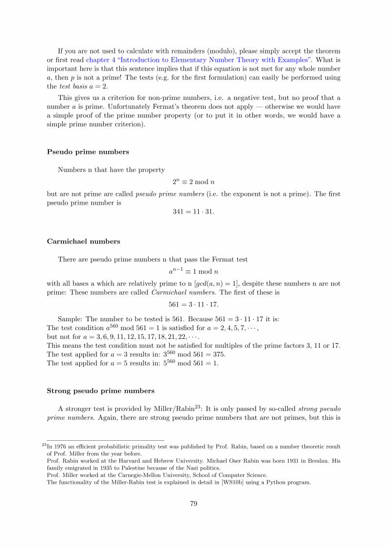
If you are not used to calculate with remainders (modulo), please simply accept the theoremor first read chapter 4 “Introduction to Elementary Number Theory with Examples”. What isimportant here is that this sentence implies that if this equation is not met for any whole numbera, then p is not a prime! The tests (e.g. for the first formulation) can easily be performed usingthe test basis a = 2.
This gives us a criterion for non-prime numbers, i.e. a negative test, but no proof that anumber a is prime. Unfortunately Fermat’s theorem does not apply — otherwise we would havea simple proof of the prime number property (or to put it in other words, we would have asimple prime number criterion).
Pseudo prime numbers
Numbers n that have the property
2n ≡ 2 mod n
but are not prime are called pseudo prime numbers (i.e. the exponent is not a prime). The firstpseudo prime number is
341 = 11 · 31.
Carmichael numbers
There are pseudo prime numbers n that pass the Fermat test
an−1 ≡ 1 mod n
with all bases a which are relatively prime to n [gcd(a, n) = 1], despite these numbers n are notprime: These numbers are called Carmichael numbers. The first of these is
561 = 3 · 11 · 17.
Sample: The number to be tested is 561. Because 561 = 3 · 11 · 17 it is:The test condition a560 mod 561 = 1 is satisfied for a = 2, 4, 5, 7, · · · ,but not for a = 3, 6, 9, 11, 12, 15, 17, 18, 21, 22, · · · .This means the test condition must not be satisfied for multiples of the prime factors 3, 11 or 17.The test applied for a = 3 results in: 3560 mod 561 = 375.The test applied for a = 5 results in: 5560 mod 561 = 1.
Strong pseudo prime numbers
A stronger test is provided by Miller/Rabin23: It is only passed by so-called strong pseudoprime numbers. Again, there are strong pseudo prime numbers that are not primes, but this is
23In 1976 an efficient probabilistic primality test was published by Prof. Rabin, based on a number theoretic resultof Prof. Miller from the year before.Prof. Rabin worked at the Harvard and Hebrew University. Michael Oser Rabin was born 1931 in Breslau. Hisfamily emigrated in 1935 to Palestine because of the Nazi politics.Prof. Miller worked at the Carnegie-Mellon University, School of Computer Science.The functionality of the Miller-Rabin test is explained in detail in [WS10b] using a Python program.
79

much less often the case than for (simple) pseudo prime numbers or for Carmichael numbers.The smallest strong pseudo prime number base 2 is
15, 841 = 7 · 31 · 73.
If you test all 4 bases, 2, 3, 5 and 7, you will find only one strong pseudo prime number up to25 · 109, i.e. a number that passes the test and yet is not a prime number.
More extensive mathematics behind the Rabin test delivers the probability that the numberexamined is prime (such probabilities are currently around 10−60).
Detailed descriptions of tests for finding out whether a number is prime can be found onWeb sites such as:
http://www.utm.edu/research/primes/mersenne.shtml
http://www.utm.edu/research/primes/prove/index.html
3.6 Special types of numbers and the search for a formula forprimes
There are currently no useful, open (i.e. not recursive) formulae known that only deliver primenumbers (recursive means that in order to calculate the function the same function is used witha smaller variable). Mathematicians would be happy if they could find a formula that leavesgaps (i.e. does not deliver all prime numbers) but does not deliver any composite (non-prime)numbers.
Ideally, we would like, for the number n, to immediately be able to obtain the n-th primenumber, i.e. for f(8) = 19 or for f(52) = 239.
Ideas for this can be found at
http://www.utm.edu/research/primes/notes/faq/p_n.html.
Cross-reference: the table under 3.10 contains the precise values for the nth prime numbersfor selected n.
For “prime number formulae” usually very special types of numbers are used. The followingenumeration contains the most common ideas for “prime number formulae”, and what our currentknowledge is about very big elements of the number series: Is their primality proven? If theirare compound numbers could their prime factors be determined?
3.6.1 Mersenne numbers f(n) = 2n − 1 for n prime
As shown above, this formula seems to deliver relatively large prime numbers but - as for n = 11[f(n) = 2, 047] - it is repeatedly the case that the result even with prime exponents is not prime.Today, all the Mersenne primes having less than around 4,000,000 digits are known (M-39):
http://yves.gallot.pagesperso-orange.fr/primes/index.html
80

3.6.2 Generalized Mersenne numbers f(k, n) = k · 2n ± 1 for n prime and ksmall prime / Proth numbers24
This first generalization of the Mersenne numbers creates the so called Proth numbers. Thereare (for small k) extremely quick prime number tests (see [Knu98]). This can be performed inpractice using software such as the Proths software from Yves Gallot:
http://www.prothsearch.net/index.html.
3.6.3 Generalized Mersenne numbers f(b, n) = bn ± 1 / The Cunninghamproject
This is another possible generalisation of the Mersenne numbers. The Cunningham projectdetermines the factors of all composite numbers that are formed as follows:
f(b, n) = bn ± 1 for b = 2, 3, 5, 6, 7, 10, 11, 12
(b is not equal to multiples of bases already used, such as 4, 8, 9).
Details of this can be found at:http://www.cerias.purdue.edu/homes/ssw/cun
3.6.4 Fermat numbers25 f(n) = 22n+ 1
As mentioned above in chapter 3.5, Fermat wrote to Mersenne regarding his assumption, thatall numbers of this type are primes. This assumption was disproved by Euler (1732). The prime641 divides f(5).26
f(0) = 220
+ 1 = 21 + 1 = 3 7→ prime
f(1) = 221
+ 1 = 22 + 1 = 5 7→ prime
f(2) = 222
+ 1 = 24 + 1 = 17 7→ prime
f(3) = 223
+ 1 = 28 + 1 = 257 7→ prime
f(4) = 224
+ 1 = 216 + 1 = 65,537 7→ prime
f(5) = 225
+ 1 = 232 + 1 = 4,294,967,297 = 641 · 6,700,417 7→ NOT prime!
f(6) = 226
+ 1 = 264 + 1 = 18,446,744,073,709,551,617= 274,177 · 67,280,421,310,721 7→ NOT prime!
f(7) = 227
+ 1 = 2128 + 1 = (see page 78) 7→ NOT prime!
Within the project “Distributed Search for Fermat Number Dividers” offered by LeonidDurman there is also progress in finding new monster primes:
http://www.fermatsearch.org/
This website links to other web pages in Russian, Italian and German.
The discovered factors can be compound integers or primes.
On February 22, 2003 John Cosgrave discovered
24Their names come from the French farmer Francois Proth (1852-1879). More famous as the Proth primes is therelated Sierpinski problem: Find all numbers k, so that k ∗ 2n + 1 is composite for all n > 0. See table 3.1.
25The Fermat prime numbers play a role in circle division. As proven by Gauss a regular p-edge can only beconstructed with the use of a pair of compasses and a ruler, when p is a Fermat prime number.
26Surprisingly this number can easily be found by using Fermat’s theorem (see e.g. [Sch06, p. 176])
81

• the largest composite Fermat number to date and
• the largest prime non-simple Mersenne number so far with 645,817 decimal digits.
The Fermat numberf(2, 145, 351) = 2(2
2,145,351) + 1
is divisible by the primep = 3 ∗ 22,145,353 + 1
At that time this prime p was the largest known prime generalized Mersenne number and the5th largest known prime number at all.
This work was done using NewPGen from Paul Jobling’s, PRP from George Woltman’s,Proth from Yves Gallot’s programs and also the Proth-Gallot group at St. Patrick’s College,Dublin.
More details are in
http://www.fermatsearch.org/history/cosgrave_record.htm
3.6.5 Generalized Fermat numbers27 f(b, n) = b2n+ 1
Generalized Fermat numbers are more numerous than Mersenne numbers of a equal size andmany of them are waiting to be discovered to fill the big gaps between the Mersenne primesalready found or still undiscovered. Progress in number theory made it possible that numbers,where the representation is not limited to the base 2, can be tested at almost the same speedthan a Mersenne number.
Yves Gallot wrote the program Proth.exe to investigate generalized Fermat numbers.
Using this program at February 16, 2003 Michael Angel discovered the largest of them tillthen with 628,808 digits, which at that time became the 5th largest known prime number:
b217
+ 1 = 62, 722131,072 + 1.
More details are in
http://primes.utm.edu/top20/page.php?id=12
3.6.6 Carmichael numbers
As mentioned above in chapter 3.5 not all Carmichael numbers are prime.
3.6.7 Pseudo prime numbers
See above in chapter 3.5.
3.6.8 Strong pseudo prime numbers
See above in chapter 3.5.
27The base of this power is no longer restricted to 2. Even more generic would be: f(b, c, n) = bcn
± 1
82
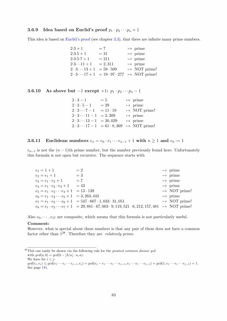
3.6.9 Idea based on Euclid’s proof p1 · p2 · · · pn + 1
This idea is based on Euclid’s proof (see chapter 3.3), that there are infinite many prime numbers.
2·3 + 1 = 7 7→ prime2·3·5 + 1 = 31 7→ prime2·3·5·7 + 1 = 211 7→ prime2·3· · ·11 + 1 = 2, 311 7→ prime2 · 3 · · · 13 + 1 = 59 · 509 7→ NOT prime!2 · 3 · · · 17 + 1 = 19 · 97 · 277 7→ NOT prime!
3.6.10 As above but −1 except +1: p1 · p2 · · · pn − 1
2 · 3− 1 = 5 7→ prime2 · 3 · 5− 1 = 29 7→ prime2 · 3 · · · 7− 1 = 11 · 19 7→ NOT prime!2 · 3 · · · 11− 1 = 2, 309 7→ prime2 · 3 · · · 13− 1 = 30, 029 7→ prime2 · 3 · · · 17− 1 = 61 · 8, 369 7→ NOT prime!
3.6.11 Euclidean numbers en = e0 · e1 · · · en−1 + 1 with n ≥ 1 and e0 := 1
en−1 is not the (n− 1)th prime number, but the number previously found here. Unfortunatelythis formula is not open but recursive. The sequence starts with
e1 = 1 + 1 = 2 7→ primee2 = e1 + 1 = 3 7→ primee3 = e1 · e2 + 1 = 7 7→ primee4 = e1 · e2 · e3 + 1 = 43 7→ primee5 = e1 · e2 · · · e4 + 1 = 13 · 139 7→ NOT prime!e6 = e1 · e2 · · · e5 + 1 = 3, 263, 443 7→ primee7 = e1 · e2 · · · e6 + 1 = 547 · 607 · 1, 033 · 31, 051 7→ NOT prime!e8 = e1 · e2 · · · e7 + 1 = 29, 881 · 67, 003 · 9, 119, 521 · 6, 212, 157, 481 7→ NOT prime!
Also e9, · · · , e17 are composite, which means that this formula is not particularly useful.
Comment:However, what is special about these numbers is that any pair of them does not have a commonfactor other than 128. Therefore they are relatively prime.
28This can easily be shown via the following rule for the greatest common divisor gcdwith gcd(a, b) = gcd(b− bb/ac · a, a).We have for i < j:gcd(ei, ej) ≤ gcd(e1 · · · ei · · · ej−1, ej) = gcd(ej − e1 · · · ei · · · ej−1, e1 · · · ei · · · ej−1) = gcd(1, e1 · · · ei · · · ej−1) = 1.See page 181.
83

3.6.12 f(n) = n2 + n+ 41
This sequence starts off very promisingly, but is far from being a proof.
f(0) = 41 7→ primef(1) = 43 7→ primef(2) = 47 7→ primef(3) = 53 7→ primef(4) = 61 7→ primef(5) = 71 7→ primef(6) = 83 7→ primef(7) = 97 7→ prime...f(33) = 1, 163 7→ primef(34) = 1, 231 7→ primef(35) = 1, 301 7→ primef(36) = 1, 373 7→ primef(37) = 1, 447 7→ primef(38) = 1, 523 7→ primef(39) = 1, 601 7→ primef(40) = 1681 = 41 · 41 7→ NOT prime!f(41) = 1763 = 41 · 43 7→ NOT prime!
The first 40 values are prime numbers (which have the obvious regularity that their differencestarts with 2 and increases by 2 each time), but the 41th and 42th values are not prime numbers. Itis easy to see that f(41) cannot be a prime number: f(41) = 412+41+41 = 41(41+1+1) = 41·43.
3.6.13 f(n) = n2 − 79 · n+ 1, 601
This function delivers prime numbers for all values from n = 0 to n = 79 .29 Unfortunatelyf(80) = 1, 681 = 11 · 151 is not a prime number. To this date, no function has been found thatdelivers more prime numbers in a row. On the other hand, each prime occurs twice (first in thedecreasing then in the increasing sequence), which means that the algorithm delivers a total of 40different prime values (these are the same ones as delivered by the function in chapter 3.6.12)30.
29See chapter 3.14, “Appendix: Examples using SageMath” for the source code to compute the table using SageMath.30Another quadratic polynom, which delivers these primes, is: f(n) = n2 − 9 · n+ 61.
Among the first 1000 sequence elements more than 50% are prime (See chapter 3.14, “Appendix: Examples usingSageMath”.).
84

f(0) = 1.601 7→ prim f(26) = 223 7→ primf(1) = 1.523 7→ prim f(27) = 197 7→ primf(2) = 1.447 7→ prim f(28) = 173 7→ primf(3) = 1.373 7→ prim f(29) = 151 7→ primf(4) = 1.301 7→ prim f(30) = 131 7→ primf(5) = 1.231 7→ prim f(31) = 113 7→ primf(6) = 1.163 7→ prim f(32) = 97 7→ primf(7) = 1.097 7→ prim f(33) = 83 7→ primf(8) = 1.033 7→ prim f(34) = 71 7→ primf(9) = 971 7→ prim f(35) = 61 7→ primf(10) = 911 7→ prim f(36) = 53 7→ primf(11) = 853 7→ prim f(37) = 47 7→ primf(12) = 797 7→ prim f(38) = 43 7→ primf(13) = 743 7→ prim f(39) = 41 7→ primf(14) = 691 7→ prim f(40) = 41 7→ primf(15) = 641 7→ prim f(41) = 43 7→ primf(16) = 593 7→ prim f(42) = 47 7→ primf(17) = 547 7→ prim f(43) = 53 7→ primf(18) = 503 7→ prim · · ·f(19) = 461 7→ prim f(77) = 1.447 7→ primf(20) = 421 7→ prim f(78) = 1.523 7→ primf(21) = 383 7→ prim f(79) = 1.601 7→ primf(22) = 347 7→ prim f(80) = 41 · 41 7→ NOT prim!f(21) = 383 7→ prim f(81) = 41 · 43 7→ NOT prim!f(22) = 347 7→ prim f(82) = 1.847 7→ primf(23) = 313 7→ prim f(83) = 1.933 7→ primf(24) = 281 7→ prim f(84) = 43 · 47 7→ NOT prim!f(25) = 251 7→ prim
3.6.14 Polynomial functions f(x) = anxn + an−1x
n−1 + · · ·+ a1x1 + a0 (ai in Z,
n ≥ 1)
There exists no such polynomial that for all x in Z only delivers prime values. For a proof ofthis, please refer to [Pad96, p. 83 f.], where you will also find further details about prime numberformulae.
This means there is no hope in looking for further formulae (functions) similar to that inchap. 3.6.12 or chap. 3.6.13.
85

3.6.15 Catalan’s Mersenne conjecture31
Catalan conjectured32 that C4 and any further term in this sequence is a prime:
C0 = 2,C1 = 2C0 − 1,C2 = 2C1 − 1,C3 = 2C2 − 1,C4 = 2C3 − 1, · · ·
This sequence is defined recursively and increases extremely quickly. Does it only consist ofprimes?
C(0) = 2 7→ primeC(1) = 22 − 1 = 3 7→ primeC(2) = 23 − 1 = 7 7→ primeC(3) = 27 − 1 = 127 7→ primeC(4) = 2127 − 1 = 170, 141, 183, 460, 469, 231, 731, 687, 303, 715, 884, 105, 727 7→ prime
It is not (yet) known whether C5 = 2C4 − 1 and all higher elements are prime. In any case,it has not been proved that this formula delivers only primes.
It seems very unlikely that C5 (or many of the larger terms) would be prime.
So this could be another example of Guy’s “law of small numbers”33.
3.6.16 Double Mersenne primes
The above Catalan-Mersenne numbers are from C2 a subset of the double Mersenne primes.34 Adouble Mersenne prime is a Mersenne prime of the form
MMp = 22p−1 − 1
where p is a Mersenne prime exponent and Mp ist a prime Mersenne number.
The first values of p for which Mp is prime are p = 2, 3, 5, 7, 13, 17, 19, 31, 61, 89, 107, 127,521, ... (see above).
MMp is known to be prime for p = 2, 3, 5, 7, and there has the according values: 7, 127,2.147.483.647, 170.141.183.460.469.231.731.687.303.715.884.105.727.35
31Eugene Charles Catalan, Belgian mathematician, May 5, 1814−Feb 14, 1894.After him, the so-called Catalan numbers A(n) = (1/(n+ 1)) ∗ (2n)!/(n!)2
= 1, 2, 5, 14, 42, 132, 429, 1430, 4862, 16796, 58786, 208012, 742900, 2674440, 9694845, ... are named.32See http://primes.utm.edu/mersenne/index.html under “Conjectures and Unsolved Problems”.33http://primes.utm.edu/glossary/page.php?sort=LawOfSmall34http://en.wikipedia.org/wiki/Catalan%E2%80%93Mersenne_number35SageMath calculates this with:
sage: for p in (2,3,5,7): Mp=(2^p)-1; MMp=(2^Mp)-1; B=is_prime(MMp); print p, Mp, MMp, B;
....:
2 3 7 True
3 7 127 True
5 31 2147483647 True
7 127 170141183460469231731687303715884105727 True
86

For p = 11, 13, 17, 19, and 31, the corresponding double Mersenne numbers are not prime.
The next candidate for the next double Mersenne prime is MM61 = 22305843009213693951 − 1.Being approximately 1.695 ∗ 10694,127,911,065,419,641, this number — like C5 — is far too large forany currently known primality test to be successfully applied.
3.7 Density and distribution of the primes
As Euclid discovered, there is an infinite number of primes. However, some infinite sets aredenser than others.
Within the set of natural numbers, there is an infinite number of even, uneven and squarenumbers. How to compare the “density” of two infinite sets is shown with even and squarenumbers.
The following proves that the even numbers are distributed more densely than square ones:36
• the size of the nth element:The nth element of the even numbers is 2n; the nth element of the square numbers is n2.Because for all n > 2: 2n < n2, the nth even number occurs much earlier than the nthsquare number.
• the numbers of values that are less than or equal to a certain maximum value x in R are:There are bx/2c such even numbers and b
√xc square numbers. Because for all x > 6 the
value bx/2c is greater than the largest integer smaller or equal to the square root of x, theeven numbers are distributed more densely.
The value of the n-th prime P (n)
Theorem 3.7.1. For large n: The value of the n-th prime P (n) is asymptotic to n · ln(n), i.e.the limit of the relation P (n)/(n · lnn) is equal to 1 if n tends to infinity.
For n > 5, P (n) lies between 2n and n2. This means that there are fewer prime numbersthan even natural numbers, but more prime numbers than square numbers.37
The number of prime numbers PI(x)
The definition for the number38 PI(x) is similar: It is the number of all primes that do notexceed the maximum value x.
Theorem 3.7.2. PI(x) is asymptotic to x/ln(x).
36Whereas in colloquial language you often can hear, that “there are more” even numbers than square ones,mathematicians say, that from both there are infinitely many, that their sets are equivalent to N (so both areinfinite and countable, i.e. one can assign to each even number and to each square number an integer), but thatthe set of even numbers is denser than the set of square numbers.
37Please refer to the table 3.1038Often, instead of PI(x) the convention Π(x) is used.
87

This is the prime number theorem. It was put forward by Legendre39 and Gauss40 butnot proved until over 100 years later.41
The tables under 3.9 show the number of prime numbers in various intervals.The distribution is graphically presented within Figure 3.9 at page 108 within the appendix 3.13.
The formulae for the prime number theorem only apply when n tends to infinity. The formulaof Gauss can be replaced by more precise formulae. For x ≥ 67:
ln(x)− 1, 5 < x/PI(x) < ln(x)− 0, 5
Given that we know PI(x) = x/ lnx only for very large x (x tending towards infinity), we cancreate the following overview:
x ln(x) x/ln(x) PI(x)(counted) PI(x)/(x/ln(x))103 6.908 144 168 1.160106 13.816 72, 386 78, 498 1.085109 20.723 48, 254, 942 50, 847, 534 1.054
For a binary number42 x of the length of 250 bits (2250 is approximately = 1.809251 ∗ 1075)it is:
PI(x) = 2250/(250 · ln 2) is approximately = 2250/173.28677 = 1.045810 · 1073.
We can therefore expect that the set of numbers with a bit length of less than 250 containsapproximately 1073 primes (a reassuring result?!).
We can also express this as follows: Let us consider a random natural number n. Then theprobability that this number is prime is around 1/ ln(n). For example, let us take numbers inthe region of 1016. Then we must consider 16 · ln 10 = 36, 8 numbers (on average) until we finda prime. A precise investigation shows: There are 10 prime numbers between 1016 − 370 and1016 − 1.
Under the heading How Many Primes Are There athttp://primes.utm.edu/howmany.html
you will find numerous other details.
Using the following Web site:https://primes.utm.edu/nthprime/
you can easily determine PI(x).
The distribution of primes43 displays several irregularities for which no “system” has yetbeen found: On the one hand, many occur closely together, like 2 and 3, 11 and 13, 809 and811, on the other hand large gaps containing no primes also occur. For example, no primes liebetween 113 and 127, 293 and 307, 317 and 331, 523 and 541, 773 and 787, 839 and 853 as wellas between 887 and 907.For details, please see:
http://primes.utm.edu/notes/gaps.html
To discover the secrets of these irregularities is precisely part of what motivates mathemati-cians.
39Adrien-Marie Legendre, French mathematician, Sep 18, 1752 − Jan 10, 1833.40Carl Friedrich Gauss, German mathematician and astronomer, Apr 30, 1777−Feb 23, 1855.41A didactical article about the prime number theorem and its application to the RSA algorithm can be found
within the series RSA & Co. at school: Modern cryptology, old mathematics, and subtle protocols: see NF part 4[WS10a]. Unfortunately these are currently only available in German.
42Number written in the binary system consists only of the digits 0 and 1.43Some visualizations (plots) of the quantity of primes in different number dimensions can be found in chapter 3.13,
“Appendix: Visualization of the quantity of primes in higher ranges”.
88
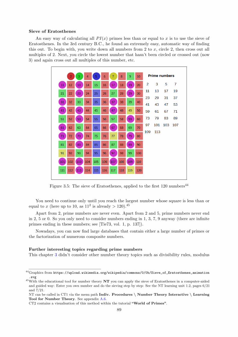
Sieve of Eratosthenes
An easy way of calculating all PI(x) primes less than or equal to x is to use the sieve ofEratosthenes. In the 3rd century B.C., he found an extremely easy, automatic way of findingthis out. To begin with, you write down all numbers from 2 to x, circle 2, then cross out allmultiples of 2. Next, you circle the lowest number that hasn’t been circled or crossed out (now3) and again cross out all multiples of this number, etc.
Figure 3.5: The sieve of Eratosthenes, applied to the first 120 numbers44
You need to continue only until you reach the largest number whose square is less than orequal to x (here up to 10, as 112 is already > 120).45
Apart from 2, prime numbers are never even. Apart from 2 and 5, prime numbers never endin 2, 5 or 0. So you only need to consider numbers ending in 1, 3, 7, 9 anyway (there are infiniteprimes ending in these numbers; see [Tie73, vol. 1, p. 137]).
Nowadays, you can now find large databases that contain either a large number of primes orthe factorization of numerous composite numbers.
Further interesting topics regarding prime numbersThis chapter 3 didn’t consider other number theory topics such as divisibility rules, modulus
44Graphics from https://upload.wikimedia.org/wikipedia/commons/0/0b/Sieve_of_Eratosthenes_animation
.svg45With the educational tool for number theory NT you can apply the sieve of Eratosthenes in a computer-aided
and guided way: Enter you own number and do the sieving step by step: See the NT learning unit 1.2, pages 6/21and 7/21.NT can be called in CT1 via the menu path Indiv. Procedures \ Number Theory Interactive \ LearningTool for Number Theory. See appendix A.6.CT2 contains a visualisation of this method within the tutorial “World of Primes”.
89

calculation, modular inverses, modular powers, modular roots, Chinese remainder theorem, EulerPhi function or perfect numbers. Some of these topics are considered in the next chapter(chapter 4).
90

3.8 Notes about primes
The following notes list some interesting theorems, conjectures and open questions about primes,but also some quaint things and overviews.
3.8.1 Proven statements / theorems about primes
• For each number n in N there are n consecutive natural numbers that are not primes. Aproof of this can be found in [Pad96, p. 79].
• Paul Erdos46 proved: Between each random number not equal to 1 and its double, there isat least one prime. He was not the first to prove this theorem, but proved it in a muchsimpler manner than those before him.
• There is a real number a such that the function f : N→ Z where n 7→ ba3nc only deliversprimes47 for all n (see [Pad96, p. 82]). Unfortunately, problems arise when we try todetermine a (see chapter 3.8.2).48
• There are arithmetic prime sequences of arbitrary length.49,50
In 1923 the famous British mathematician Hardy51 compiled the conjecture, that thereare arithmetic sequences of arbitrary length, which consist of primes only. This conjecturewas proven in 2004 by two young American mathematicians.
At some point every school child learns about arithmetic number series. These are sequencesof numbers, for which the difference between any 2 consecutive numbers is equal or constant(an arithmetic sequence must have at least three elements but can also have indefinitelymany). In the sample sequence 5, 8, 11, 14, 17, 20 the difference between the series’selements is 3 and the length of the sequence is 6.
Arithmetic series have been known for millennia and one would think they have no moresecrets. They get more interesting again, if we impose additional constraints on the serie’selements - as the prime example shows.
E.g. 5, 17, 29, 41, 53 is an arithmetic prime series which consists of 5 elements and thedifference between the elements is always 12.
The sequence is not extendable - the next would be 65, but 65 is not prime (65 is theproduct of 5 and 13).
How many elements are possible within an arithmetic prime number sequence? Around1770 the French Joseph-Louis Lagrange and the British Edward Waring investigated
46Paul Erdos, Hungarian mathematician, Mar 26, 1913−Sep 20, 1996.47The Gauss bracket bxc of a real number x is defined via: bxc is the next integer less or equal x.48If someone knows how to prove this, we are very interested to learn about this. Friedhelm Padberg told us, he
doesn’t have his prove any more.49Sources:
- http://primes.utm.edu/glossary/page.php?sort=ArithmeticSequence Original source- http://en.wikipedia.org/wiki/Primes_in_arithmetic_progression- http://en.wikipedia.org/wiki/Problems_involving_arithmetic_progressions- http://en.wikipedia.org/wiki/Cunningham_chain- German magazine GEO 10 / 2004: “Experiment mit Folgen”- http://www.faz.net “Hardys Vermutung – Primzahlen ohne Ende” by Heinrich Hemme (July 06, 2004)
50Arithmetic sequences with k primes are called prime arithmetic progressions and therefore their abbreviation isPAP-k or AP-k.
51Godfrey Harold Hardy, British mathematician, Feb 7, 1877−Dec 1, 1947.
91
this question. In 1923 the famous British mathematician Godfrey Harold Hardy andhis colleague John Littlewood theorized, that there is no upper limit for the number ofelements. But they could not prove this. In 1939 more progress was achieved: The Dutchmathematician Johannes van der Corput was able to prove that there are infinitely manydifferent arithmetic prime number sequences with exactly three elements. Two examplesare 3, 5, 7 and 47, 53, 59.
The longest arithmetic prime number sequence known today contains 25 elements. Thetable 3.3 lists the longest currently known arithmetic prime number sequences with minimaldifference52.
As a team, the two young53 mathematicians Ben Green and Terence Tao, were able in 2004to prove Hardy’s conjecture, which had puzzled mathematicians for over 80 years: It states,that for any arbitrary length there exists an arithmetic prime number series. Additionallythey managed to prove, that for any given length there are infinitely many different series.
Green and Tao intended to proof that there are infinitely many arithmetic sequences oflength four. For this they considered sets of numbers consisting of primes and so called“near primes”. These are numbers with a small set of divisors like numbers which are theproduct of two primes - these numbers are called “half primes”. Thus they managed toconsiderably simplify their work because about near primes there already existed a lot ofuseful theorems. Finally they discovered that the results of their theorem were far morereaching than they had assumed and so they were able to prove Hardy’s conjecture.
Any one who believes that it is easy to use Green’s and Tao’s 49 page proof to computearithmetic prime number series of arbitrary length will soon become disappointed, becausethe proof is non-constructive. It is a so called proof of existence. This means that thesemathematicians have shown “only” that these series exist, but not how to find them inpractice.
This means that in the set of the natural numbers there is e.g. a series of one billionprimes, which all have the same distance; and there are infinitely many of them. But thesesequences lie extremely far beyond the numbers we usually use (“far outside”).
52In the opposite, http://en.wikipedia.org/wiki/Primes_in_arithmetic_progression lists the “largest knownAP-k”. Therefore, there the last sequence element is a prime as big as possible.However, table 3.3 lists the sequences which have the smallest known difference for a given length.
53Hardy wrote in his memoirs in 1940, that mathematics - more than all other arts and sciences - is an activity foryoung people.At that time, 27-years-old Ben Green from the University of British Columbia in Vancouver and 29-year-oldTerence Tao from the University of California in Los Angeles seem to confirm Hardy.
92

Elements First element Distance When Discovered byDigits
3 3 21
4 5 62
5 5 62
6 7 30 1909 G. Lenaire3
7 7 150 1909 G. Lenaire3
.......
21 28,112,131,522,731,197,609 9,699,690 2008 Jaroslaw Wroblewski= 19# 20
22 166,537,312,120,867 96,599,212,710 2006 Markus Frind= 9,959·19# 15
23 403,185,216,600,637 2,124,513,401,010 2006 Markus Frind,= 9,523·23# 15
24 515,486,946,529,943 30,526,020,494,970 2008 Raanan Chermoni,= 136,831·23# 16 Jaroslaw Wroblewski
25 6,171,054,912,832,631 81,737,658,082,080 2008 Raanan Chermoni,= 366,384·23# 16 Jaroslaw Wroblewski
Table 3.3: Arithmetic prime number sequences with minimal difference (as of Aug. 2012)
93
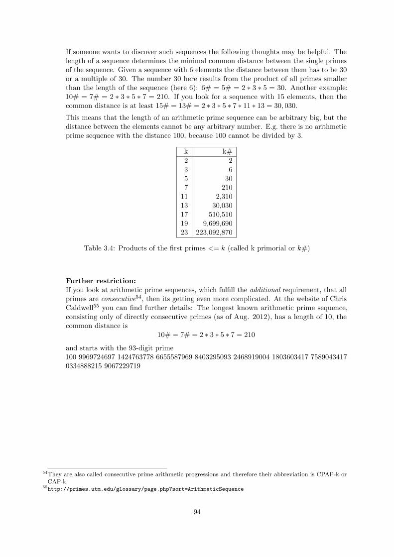
If someone wants to discover such sequences the following thoughts may be helpful. Thelength of a sequence determines the minimal common distance between the single primesof the sequence. Given a sequence with 6 elements the distance between them has to be 30or a multiple of 30. The number 30 here results from the product of all primes smallerthan the length of the sequence (here 6): 6# = 5# = 2 ∗ 3 ∗ 5 = 30. Another example:10# = 7# = 2 ∗ 3 ∗ 5 ∗ 7 = 210. If you look for a sequence with 15 elements, then thecommon distance is at least 15# = 13# = 2 ∗ 3 ∗ 5 ∗ 7 ∗ 11 ∗ 13 = 30, 030.
This means that the length of an arithmetic prime sequence can be arbitrary big, but thedistance between the elements cannot be any arbitrary number. E.g. there is no arithmeticprime sequence with the distance 100, because 100 cannot be divided by 3.
k k#
2 23 65 307 210
11 2,31013 30,03017 510,51019 9,699,69023 223,092,870
Table 3.4: Products of the first primes <= k (called k primorial or k#)
Further restriction:If you look at arithmetic prime sequences, which fulfill the additional requirement, that allprimes are consecutive54, then its getting even more complicated. At the website of ChrisCaldwell55 you can find further details: The longest known arithmetic prime sequence,consisting only of directly consecutive primes (as of Aug. 2012), has a length of 10, thecommon distance is
10# = 7# = 2 ∗ 3 ∗ 5 ∗ 7 = 210
and starts with the 93-digit prime100 9969724697 1424763778 6655587969 8403295093 2468919004 1803603417 75890434170334888215 9067229719
54They are also called consecutive prime arithmetic progressions and therefore their abbreviation is CPAP-k orCAP-k.
55http://primes.utm.edu/glossary/page.php?sort=ArithmeticSequence
94

3.8.2 Unproven statements/ conjectures/ open questions about primes56
• Goldbach57 conjectured: Every even natural number greater than 2 can be represented asthe sum of two prime numbers.58
• Riemann59 put forward an important, but still unproved hypothesis60 about the location ofthe nontrivial zeros of the Riemann zeta function. A consequence is an improved estimationwithin the prime number theorem (distribution of primes).
• Benford’s law61,62 does not apply to primes.
According to Benford’s law, also called the first-digit law, the single digits in lists ofnumbers from many (but not all) real-life sources of data, are distributed in a non-uniformway. Especially the leading digit is much more often the digit 1 than any other digit.
Which empirical data applies to this “law” ist not completely clear yet. Timo Eckhardtanalyzed in his thesis in 2008 extensively attributes of prime numbers. For example, allprimes until 7,052,046,499 were described with different bases of the positional notation.
Comparing the bases 3 to 10 the deviation from Benford’s law was lowest with base 3.Comparing the first digit for base 10 all digits are almost equally distributed. Analyzingbigger bases showed strong differences.
• The proof (mentioned above in chapter 3.8.1) of the function f : N → Z with n 7→ ba3nconly guarantees the existence of such a number a. How can we determine this number aand will it have a value, making the function also of some practical interest?
• Is there an infinite number of Mersenne prime numbers?
• Is there an infinite number of Fermat prime numbers?
• Does a polynomial time algorithm exist for calculating the prime factors of a number (see[KW97, p. 167])? This question can be divided into the three following questions:
– Does a polynomial time algorithm exist that decides whether a number is prime?This question has been answered by the AKS algorithm (see chapter 4.11.5.3, “Primesin P”: Primality testing is polynomial).
56Marcus du Sautoy, a professor of mathematics in Oxford, describes in his popular science book “The Music ofthe Primes”, how some of the most brilliant mathematicians looked at different aspects of prime numbers. Heintroduces these people (especially Gauß, Euler, Riemann, Ramanujan, Godel, and Connes) and then focuses onthe Riemann hypothesis. See [dS05].Simple explanations and further references about the Riemann hypothesis can also be found in RSA & Co. atschool, NF part 4 [WS10a].
57Christian Goldbach, German mathematician, Mar 18, 1690−Nov 20, 1764.58Please compare chapter 3.8.3.59Bernhard Riemann, German mathematician, Sep 17, 1826−Jul 20, 1866.60http://en.wikipedia.org/wiki/Riemann_hypothesis61http://en.wikipedia.org/wiki/Benford%27s_law,http://arxiv.org/PS_cache/arxiv/pdf/0906/0906.2789v1.pdf.
62Two good didactical articles in German about applications of Benford’s law are:– Rudeger Baumann: “Ziffernanalyse zwecks Betrugsaufdeckung — Beispiel fur kompetenzorientierten und
kontextbezogenen Informatikunterricht”,in LOGIN, Informatische Bildung und Computer in der Schule, No. 154/155, 2008, p. 68-72
– Norbert Hungerbuhler: “Benfords Gesetz uber fuhrende Ziffern”, March 2007,https://www.ethz.ch/content/dam/ethz/special-interest/dual/educeth-dam/documents/Unterric
htsmaterialien/mathematik/Benfords%20Gesetz%20%C3%BCber%20f%C3%BChrende%20Ziffern%20(Arti
kel)/benford.pdf
95

– Does a polynomial time algorithm exist that calculates for a composite number fromhow many prime factors it is made up (without calculating these factors)?
– Does a polynomial time algorithm exist that calculates for a composite number n anon-trivial (i.e. other than 1 and n) factor of n?63
At the end of chapter 4.11.4, section RSA-200 you can see the limits for which numbersthe current algorithms for primality testing and for factorization deliver good results.
3.8.3 The Goldbach conjecture
Here we will have a closer look at what is called the Goldbach conjecture64.
3.8.3.1 The weak Goldbach conjecture65
Goldbach conjectured in 1742 within a letter to the mathematician Euler:
Every odd natural number greater than 5 can be represented as the sum of exactly threeprime numbers.
Samples: 7 = 3 + 2 + 2 or 27 = 19 + 5 + 3 or 27 = 17 + 5 + 5
This conjecture ist still (since more than 250 years) assumed unproven.
Computers have verified the weak Goldbach conjecture for all odd natural numbers up to:4 ∗ 1018 (simple check at April 2012) and 4 ∗ 1017 (double check at May 2013).66
Previous results proved, that the weak Goldbach conjecture is true for all odd naturalnumbers larger e3100 ≈ 2× 101346.
As with many famous conjectures in mathematics, there are also a number of purportedproofs of the Goldbach conjecture, none accepted by the mathematical community yet.67
A preliminary work for a prove could be the prove published recently68 by Terence Tao fromthe University of California. He proved that every odd natural number greater than 1 can berepresented as the sum of at most five prime numbers.
Considerable work has been done on Goldbach’s weak conjecture, culminating in a 2013claim by Harald Helfgott to fully prove the conjecture for all odd integers greater than 7.69
63Please compare chapters 4.11.5.1 and 4.11.4.64http://en.wikipedia.org/wiki/Goldbach%27s_conjecture65It is also known as the odd or ternary Goldbach conjecture.66See http://sweet.ua.pt/tos/goldbach.html by Tomas Oliveira e Silva67One of them is in the paper from Shan-Guang Tan, submitted on 16 Oct 2011 (v1), last revised 20 May 2016
(v19) which claims to even proof the strong Goldbach conjecture.v1 has the title “A proof of the Goldbach conjecture”.v19 has the title “On the representation of even numbers as the sum and difference of two primes and therepresentation of odd numbers as the sum of an odd prime and an even semiprime and the distribution of primesin short intervals”.See http://arxiv.org/abs/1110.3465.
68http://arxiv.org/abs/1201.6656, submitted on 31 Jan 2012 (v1), last revised 3 Jul 2012 (v4)69Helfgott, H.A. (2013): “Major arcs for Goldbach’s theorem”. http://arxiv.org/abs/1305.2897.
v4 of his 79 pages paper (14 Apr 2014) states, that the proof works starting at 1029 (instead of 1030). And for allnumbers up to 1030 he claims, that he and David Platt proved at the computer that the weak Goldbach is valid.
96
3.8.3.2 The strong Goldbach conjecture70
Goldbach’s strong prime number hypothesis was formulated by Euler after a mail exchange withGoldbach. This is now called the Goldbach conjecture:
Every even natural number greater than 2 can be represented as the sum of exactly twoprime numbers.
Samples of Goldbach partitions: 8 = 5 + 3 or 28 = 23 + 5
Computers have once verified71 the Goldbach conjecture for all even numbers up to 4 ∗ 1018 (asat May 2013), but no general proof has yet been found.72,73,74
As bigger an even number is, as more such binary Goldbach partitions can be found – inaverage: For 4 there is only one partition 2 + 2; for 16 there are two, 3 + 13 and 5 + 11. With100 there are six such partitions: 3 + 97, 11 + 89, 17 + 83, 29 + 71, 41 + 59, 47 + 53.75
3.8.3.3 Interconnection between the two Goldbach conjectures
If the strong Goldbach conjectures holds, then also the weak is true (so the strong implies theweak conjecture).
The proof for this is relativly simple:Prerequisite: u is an odd number bigger than 5.Each such odd number u can be written as sum u = (u− 3) + 3. The first summand then is even
http://truthiscool.com/prime-numbers-the-271-year-old-puzzle-resolved.http://www.newscientist.com/article/dn23535-proof-that-an-infinite-number-of-primes-are-
paired.html#.UgwhOpL0Ek0.http://www.spiegel.de/wissenschaft/mensch/beweis-fuer-schwache-goldbachsche-vermutung-a-
901111.html.70It is also known as the even or binary Goldbach conjecture.71It is generally accepted today, that the Goldbach conjecture is true, i. e. valid for all even natural numbers
greater than 2. In 1999, mathematician Jorg Richstein from the computer sciences institute at the University ofGiessen, studied even numbers up to 400 billion (4 ∗ 1014) and found no contradictory example ([Ric01]).In the meantime further progress was made: Seehttp://sweet.ua.pt/tos/goldbach.html by Tomas Oliveira e Silva,http://en.wikipedia.org/wiki/Goldbach’s_conjecture,http://primes.utm.edu/glossary/page.php/GoldbachConjecture.html.Nevertheless, this does not provide us with general proof.The fact is that despite all efforts, Goldbach’s conjecture has to date not been proven. This leads one to believethat since the pioneer work of the Austrian mathematician Kurt Godel is well-known, not every true mathematicaltheorem is provable (see https://www.mathematik.ch/mathematiker/goedel.php). Perhaps Goldbach’s conjec-ture was correct, but in any case the proof will never be found. Conversely, that will presumably also remainunproven.
72The English publisher Faber and the American publisher Bloomsbury issued in 2000 the 1992 published book“Uncle Petros and Goldbach’s Conjecture” by Apostolos Doxiadis. It’s the story of an old maths professor whofails to prove a more than 250 year old puzzle. To boost the sales figures the English and American publishershave offered a prize of 1 million USD, if someone can prove the conjecture – which should be published by 2004 ina well-known mathematical journal.Surprisingly only British and American citizens are allowed to participate.
73The theorem which has come closest so far to Goldbach’s conjecture was proved by Chen Jing-Run in 1966 in away which is somewhat hard to understand: Each even integer greater than 2 is the sum of one prime and of theproduct of two primes. E.g.: 20 = 5 + 3 ∗ 5.Most of the research about the Goldbach conjecture is collected in the book: “Goldbach Conjecture”, ed. WangYuan, 1984, World scientific Series in Pure Maths, Vol. 4.
74Especially this conjecture makes it clear, that even today we do not have a complete understanding of the deeperconnections between addition and multiplication of natural numbers.
75Progress in research about the Goldbach conjectures is often a topic in mathematical press column, like http:
//oumathclub.wordpress.com/.
97
and >= 4, so it fullfils the prerequisite of the strong Goldbach conjecture, and can be written assum of two primes p1 und p2 (p1 and p2 are not necessarily different). So we found a partition ofu into the three primes p1, p2 and 3. This means, its always possible to find such a sum, whereone of the primes is the number 3.
Similarily easy it can be shown, that the weak Goldbach conjecture implies the abovementioned conjecture from Terence Tao (both hold for odd numbers):
• For odd numbers u > 5 directly the weak Goldbach conjecture implies that the sum consitsat most of five primes.
• For the remaining odd numbers 3 and 5 you can directly check it:3 = 3 (the “sum” has only one and therefore at most five prime summands);5 = 2 + 3 (the sum has two and therefore at most five prime summands).
3.8.4 Open questions about twin primes and cousin primes
Twin primes are prime numbers whose difference is exactly 2. Examples include 5 and 7, or 101and 103, or 1, 693, 965 · 266,443 ± 1.
The biggest known twin pair is
3, 756, 801, 695, 685 · 2666,669 ± 1
with 200, 700 decimal digits (found in December 2011).76
Open questions are:
• What is the number of twin primes: Are there infinitely many or only a limited num-ber?77,78,79
• Does a formula exist for calculating the number of twin primes per interval?
In the following two major milestones are explained which may allow to come closer to the riddle.
3.8.4.1 GPY 2003
A big step towards the solution of this problem was made by Dan Goldston, Janos Pintz andCem Yildirim in 2003.80 The three mathematicians were investigating the distribution of prime
76http://primes.utm.edu/primes, http://www.primegrid.com/download/twin-666669.pdf77Remark: Triplet primes, however, only occur once: 3, 5, 7. For all other sets of three consecutive odd numbers,
one of them is always divisible by 3 and thus not a prime.78The conjecture that there are infinite many twin primes is not obvious. It’s known, that for large numbers in
average the expected gap between primes is constantly growing and circa 2.3 times the number of decimal digits.For example, among 100-digit decimal numbers the expected gap between primes is in average 230. But thisstatement is true just on average – often the gap is much bigger, often much smaller.
79http://en.wikipedia.org/wiki/Twin_Prime_Conjecture80D. A. Goldston: “Gaps Between Primes”http://www.math.sjsu.edu/~goldston/OberwolfachAbstract.pdf
See also:• D. A. Goldstone: “Are There Infinitely Many Twin Primes?”
http://www.math.sjsu.edu/~goldston/twinprimes.pdf
• K. Soundararajan: “Small Gaps Between Prime Numbers: The Work Of Goldston-Pintz-Yildirim”http://www.ams.org/bull/2007-44-01/S0273-0979-06-01142-6/S0273-0979-06-01142-6.pdf
98

numbers. They could proof, that
lim infn→∞
pn+1 − pnlog pn
= 0,
where pn denotes the n-th prime number.This means that the smallest limit point (lim inf) of the sequence pn+1−pn
log pnequals zero.
A point is called limit point of a sequence, if there lie in any arbitraril small neighbourhood ofthat point infinitely many elements of the sequence.log pn is about the average distance between the prime pn and the next prime pn+1.Hence, the term above implies, that there are infinitely many consecutive primes with a gapbetween them which is arbitrarily small compared to the expected average gap.
Moreover, it was proofed, that
pn+1 − pn < (log pn)8/9
holds true for infinitely many primes81.
3.8.4.2 Zhang 2013
In May 2013 the results of Yitang Zhang became known.82 Zhang proved, that there are infinitelymany “cousin primes”, or more concretely that there is some number H smaller than 70 millionsuch that there are inifinitely many pairs of primes that differ by H.83,84,85
Those results could be the basis for the proof, that infinitely many twin primes exist.
81c’t magazine 2003, no. 8, page 5482Erica Klarreich (May 19, 2013): “Unheralded Mathematician Bridges the Prime Gap”https://www.simonsfoundation.org/quanta/20130519-unheralded-mathematician-bridges-the-prime-
gap/83Whereas the gap between the primes of a twin prime is exactly 2, cousin primes do denote two primes, which have
a gap between them, which has a value of a bigger, even, but finite number H.84This is close to the conjecture stated in 1849 by the French mathematician Alphonse de Polignac that there are
infinitely many prime pairs for any possible even finite gap, not just 2.85In the meantime this minimal gap H of 70 millions was improved in further work. The according progress is
documented in the Polymath8 project (massively collaborative online mathematical projects): “Bounded gapsbetween primes”. The best known value of H was 4680 (as of August 2013) and is till now (as of April 2014) 2460– this is a good progress compared to 70 million, but far away from 2.See http://michaelnielsen.org/polymath1/index.php?title=Bounded_gaps_between_primes
99

3.8.5 Quaint and interesting things around primes86
Primes are not only a very active and serious research area in mathematics. Also a lot of peoplethink about them in their free time and outside the scientific research.
3.8.5.1 Recruitment at Google in 2004
In summer 2004 the company Google used the number e to attract potential employees.87,88
On a prominent billboard in California’s Silicon Valley on July 12 there appeared the followingmysterious puzzle:
(first 10 digit prime in consecutive digits of e).com
Finding the first 10 digit prime in the decimal expansion of e is not easy, but with varioussoftware tools, one can determine that the answer is
7, 427, 466, 391
Then if you visited the website www.7427466391.com, you were presented with an even moredifficult puzzle. Figuring this second puzzle out took you to a web page that asks you, to submityour CV to Google. The ad campaign got high attention.
Presumably Google’s conceit was that if you’re smart enough to solve the puzzles, you’resmart enough to work for them. Of course some days after the launch, anyone who really wantedto discover the answers without incurring a headache could merely do a Google search for them,since many solvers immediately posted their solutions online.89
3.8.5.2 Contact [movie, 1997] – Primes helping to contact aliens
The movie, directed by Robert Zemeckis, originated from Carl Sagan’s book with the same title.
After years of unavailing search the radio astronomer Dr. Ellie Arroway (Jodie Foster)discovers signals from the solar system Vega, 26 light years away. These signals contain theprimes in the right order and without a gap. This makes the hero confident, that this messageis different from the radio signals which permanently hit earth and which are random and ofcosmic origin (radio galaxies, pulsars). In an unmasking scene a politician asks her after that,why these intelligent aliens didn’t just speak English ...
Doing communication with absolute strange and unknown beings from deep space is veryhard especially because of 2 reasons: First, the big distance and therefore the long transfer
86Further curious things about primes may be found at:- http://primes.utm.edu/curios/home.php- http://www.primzahlen.de.
87The base of the natural logarithm e is approximately 2.718 281 828 459. This is one of the most importantnumbers in all of mathematics like complex analysis, finance, physics and geometry. Now it was used the firsttime – as far as I know – for marketing or recruitment.
88Most of this information is taken from the article “e-number crunching” by John Allen Paulos in TheGuardian,Sept. 30, 2004, and from the web:- https://mkaz.tech/google-billboard-problems.html- http://epramono.blogspot.com/2004/10/7427466391.html- http://mathworld.wolfram.com/news/2004-10-13/google/.
89The second level of the puzzle, which involved finding the 5th term of a given number sequence had nothing to dowith primes any more.
100

time make it impossible to exchange within an average lifetime more than one message in eachdirection. Secondly the first contact must give the receiver of the radio signals a good chanceto notice the message and to categorize it as something from intelligent beings. Therefore thealiens send numbers at the beginning of their message, which can be considered as the easiestpart of any higher language, and which are not too trivial: So they chose the sequence of primes.These special numbers play such a fundamental role in mathematics that one can assume thatthey are well known to each species who has the technical know-how to receive radio waves.
The aliens then send a plan to build a mysterious machine ...
101
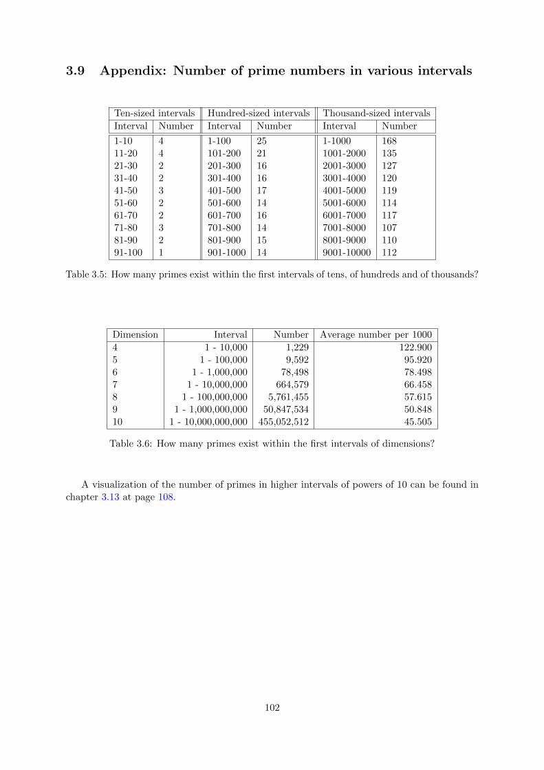
3.9 Appendix: Number of prime numbers in various intervals
Ten-sized intervals Hundred-sized intervals Thousand-sized intervals
Interval Number Interval Number Interval Number
1-10 4 1-100 25 1-1000 16811-20 4 101-200 21 1001-2000 13521-30 2 201-300 16 2001-3000 12731-40 2 301-400 16 3001-4000 12041-50 3 401-500 17 4001-5000 11951-60 2 501-600 14 5001-6000 11461-70 2 601-700 16 6001-7000 11771-80 3 701-800 14 7001-8000 10781-90 2 801-900 15 8001-9000 11091-100 1 901-1000 14 9001-10000 112
Table 3.5: How many primes exist within the first intervals of tens, of hundreds and of thousands?
Dimension Interval Number Average number per 1000
4 1 - 10,000 1,229 122.9005 1 - 100,000 9,592 95.9206 1 - 1,000,000 78,498 78.4987 1 - 10,000,000 664,579 66.4588 1 - 100,000,000 5,761,455 57.6159 1 - 1,000,000,000 50,847,534 50.84810 1 - 10,000,000,000 455,052,512 45.505
Table 3.6: How many primes exist within the first intervals of dimensions?
A visualization of the number of primes in higher intervals of powers of 10 can be found inchapter 3.13 at page 108.
102

3.10 Appendix: Indexing prime numbers (n-th prime number)
Index Precise value Rounded value Comment
1 2 22 3 33 5 54 7 75 11 116 13 137 17 178 19 199 23 2310 29 29100 541 5411,000 7,917 7,917664,559 9,999,991 9.99999E+06 All prime numbers up to 1E+07 were
known at the beginning of the 20thcentury.
1E+06 15,485,863 1.54859E+076E+06 104,395,301 1.04395E+08 This prime was discovered in 1959.1E+07 179,424,673 1.79425E+081E+09 22,801,763,489 2.28018E+101E+12 29,996,224,275,833 2.99962E+13
Table 3.7: List of particular n-th prime numbers P(n)
Comment:With gaps, extremely large prime numbers were discovered at an early stage.
Web links:https://primes.utm.edu/nthprime/
https://primes.utm.edu/notes/by_year.html.
103

3.11 Appendix: Orders of magnitude / dimensions in reality
In the description of cryptographic protocols and algorithms, numbers occur that are so large orso small that they are inaccessible to our intuitive understanding. It may therefore be useful toprovide comparative numbers from the real world around us so that we can develop a feelingfor the security of cryptographic algorithms. Some of the numbers listed below originate from[Sch96b] and [Sch96a, p.18].
Probability that you will be hijacked on your next flight 5.5 · 10−6
Annual probability of being hit by lightning 10−7
Probability of 6 correct numbers in the lottery 7.1 · 10−8
Risk of being hit by a meteorite 1.6 · 10−12
Time until the next ice age (in years) 14, 000 = (214)Time until the sun dies (in years) 109 = (230)Age of the earth (in years) 109 = (230)Age of the universe (in years) 1010 = (234)Number of molecules within one waterdrop 1020 = (263)Number of bacteria living on earth 1030.7 = (2102)Number of the earth’s atoms 1051 = (2170)Number of the sun’s atoms 1057 = (2190)Number of atoms in the universe (without dark material) 1077 = (2265)Volume of the universe (in cm3) 1084 = (2280)
Table 3.8: Likelihoods and dimensions from physics and everyday life
104
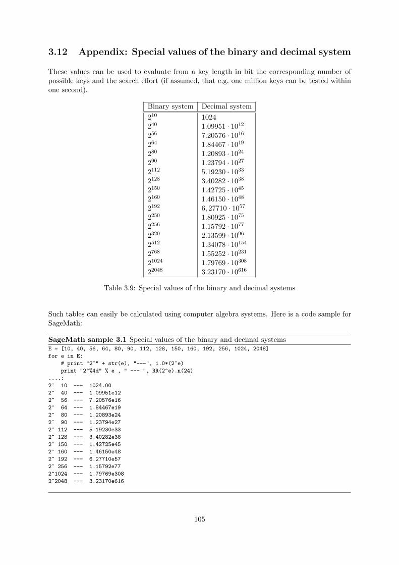
3.12 Appendix: Special values of the binary and decimal system
These values can be used to evaluate from a key length in bit the corresponding number ofpossible keys and the search effort (if assumed, that e.g. one million keys can be tested withinone second).
Binary system Decimal system
210 1024240 1.09951 · 1012
256 7.20576 · 1016
264 1.84467 · 1019
280 1.20893 · 1024
290 1.23794 · 1027
2112 5.19230 · 1033
2128 3.40282 · 1038
2150 1.42725 · 1045
2160 1.46150 · 1048
2192 6, 27710 · 1057
2250 1.80925 · 1075
2256 1.15792 · 1077
2320 2.13599 · 1096
2512 1.34078 · 10154
2768 1.55252 · 10231
21024 1.79769 · 10308
22048 3.23170 · 10616
Table 3.9: Special values of the binary and decimal systems
Such tables can easily be calculated using computer algebra systems. Here is a code sample forSageMath:
SageMath sample 3.1 Special values of the binary and decimal systemsE = [10, 40, 56, 64, 80, 90, 112, 128, 150, 160, 192, 256, 1024, 2048]
for e in E:
# print "2^" + str(e), "---", 1.0*(2^e)
print "2^%4d" % e , " --- ", RR(2^e).n(24)
....:
2^ 10 --- 1024.00
2^ 40 --- 1.09951e12
2^ 56 --- 7.20576e16
2^ 64 --- 1.84467e19
2^ 80 --- 1.20893e24
2^ 90 --- 1.23794e27
2^ 112 --- 5.19230e33
2^ 128 --- 3.40282e38
2^ 150 --- 1.42725e45
2^ 160 --- 1.46150e48
2^ 192 --- 6.27710e57
2^ 256 --- 1.15792e77
2^1024 --- 1.79769e308
2^2048 --- 3.23170e616
105

3.13 Appendix: Visualization of the quantity of primes inhigher ranges
The distribution of primes
Between 1 and 10 there are 4 primes. Between 103 and 104 there are already 1061 primes. Inthe interval [109, 1010] lie 404, 204, 977 ≈ 4 · 108 primes, and in the interval from 1019 to 1020
there are 1, 986, 761, 935, 284, 574, 233 ≈ 1, 9 · 1018 primes.90
Why is the difference between the number of primes in the different intervals so big, althoughthe boundaries of the intervals differ only by value 1 of the exponent of the power of 10?
The prime number theorem
The number PI(x) of primes up to a given number x can approximately be determined by aformula, derived from the so called prime number theorem (see chapter 3.7). PI(x) denotes thenumber of primes which are smaller or equal to x. Then the formula is
PI(x) ∼ x
lnx.
Note, that this formula only gives an approximation of the number of primes smaller or equalto x. It’s getting more exact as the number x increases.In the following we are using the prime number theorem to examine the distribution of primes.
To understand, why the number of primes is growing so rapidly, although the boundaries ofthe intervals only differ by the exponent 1, let’s have a closer look to both components of theright side of the formula: x and lnx.
The functions x and 10x
The function x is a straight line. It is shown in figure 3.6a on page 107.In the next step the function of the boundaries of the intervals are drawn in figure 3.6b on page107. To get an idea of how the functions look like, the domain of definition was chosen to befrom 0 to 1010 and from 0 to 10, respectively. You can see, that with increasing exponent x thenumbers grow stronger.
The function lnx
In comparison to that we consider the function lnx. The left picture of figure 3.7 on page 107shows the graph with the domain of definition from 1 to 100. On the right picture the domainof definition was chosen between 1 and 1010.One can see that the values of the function lnx grow slowly compared to the growth of thefunction x. This is visualizd by the graph of both functions in one picture shown in figure 3.8 onpage 107. In addition to that the graph of the function x
lnx was drawn in the same figure.
90http://en.wikipedia.org/wiki/Prime_number_theorem
106

(a) x (b) 10x
Figure 3.6: Graph of the functions x and 10x
(a) (b)
Figure 3.7: Graph of the function lnx till 100 and till 1010
Figure 3.8: The functions x (blue), lnx (red) and xlnx (green)
The function PI(x) = xlnx
The function xlnx consists of the function x as the numerator and the function lnx in the
denominator, which, in comparison to x, increases very slowly. Compared to the number x itself,the number of primes less or equal to x is small. But still, x
lnx is an increasing function as youcan see in figure 3.8 on page 107.
107

The number of primes in the different intervals
Figure 3.9 visualizes how the number of primes in the intervals [1, 10x] and [10x−1, 10x] behave.To calculate it faster, the result of the approximation function is used (not the exact numberslike in the tables in chapter 3.9).
Here for each base 10 exponent two bars are drawn: 10x
ln 10x and 10x
ln 10x −10x−1
ln 10x−1 : The left chartshows the values for the exponents x from 1 to 5, and the right one for x from 1 to 10, where xis the base 10 exponent.
The blue bars represent the overall number of primes up to 10x. The red bars show howmany primes accrue in the interval [10x−1, 10x], respectively. This makes clear, that the numberof primes in intervals of higher exponents keeps growing quite fast.
(a) (b)
Figure 3.9: Numbers of primes in the interval [1, 10x] (blue) and in the interval [10x−1, 10x] (red)for different exponents x
A table containing the number of primes in some dedicated intervals can be found in chapter3.9 at page 102: For example, within the interval [1, 104] there are 1229 primes; thereof are inthe interval [103, 104] 1229 - 168 = 1061 primes.
Theory about the prime number theorem and the function PI(x) can be found in chapter 3.7.
108

SageMath sample 3.2 Generation of the graphs of the three functions x, log(x) and x/log(x)
# Definition of function f(x)=x and plots for the domains from 0 to 10^10 and 0 to 100
sage: def f(x):return x
....:
sage: F=plot(f,(0,10^10))
sage: F.plot()
sage: F2=plot(f,(1,100))
sage: F2.plot()
# Definition of function g(x)=10^x and plots for the domain from 0 to 10
sage: def g(x): return 10^x
....:
sage: G=plot(g,(0,10))
sage: G.plot()
# Definition of function h(x)=log(x) and plots for the domains from 1 to 100 and 1 to 10^10
sage: def h(x): return log(x)
....:
sage: H=plot(h,(1,100),color="red")
sage: H.plot()
sage: H2=plot(h,(1,10^10),color="red")
sage: H2.plot()
# Definition of function k(x)=x/log(x) and plots for the domain from 2 to 100
sage: def k(x): return x/log(x)
....:
sage: K=plot(k,(2,100),color="green")
sage: K.plot()
# Plots of the functions f, k and h for the domain of definition up to 100
sage: F2+K+H
# Generation of the data for the bar charts ..........................
# Determination of the number of primes in the interval [1,10]
sage: pari(10).primepi()-pari(1).primepi()
4
# Determination of the number of primes in the interval [10^3,10^4]
sage: pari(10**4).primepi()-pari(10**3).primepi()
1061
# Determination of the number of primes in the interval [10^8,10^9]
sage: pari(10**9).primepi()-pari(10**8).primepi()
45086079
# (for 10^10: OverflowError: long int too large to convert)
109

3.14 Appendix: Examples using SageMath
Below is SageMath source code related to contents of the chapter 3 (“Prime Numbers”).
3.14.1 Some basic functions about primes using SageMath
This part of the appendix contains SageMath code, to perform some simple computations aboutprimes.91
SageMath sample 3.3 Some basic functions about primes
# primes (general commands)
# The set of prime numbers
sage: P=Primes(); P
Set of all prime numbers: 2, 3, 5, 7, ...
# Returns the next prime number
sage: next_prime(5)
7
# Returns how many primes <=x are there
sage: pari(10).primepi()
4
# Returns the first x primes
sage: primes_first_n(5)
[2, 3, 5, 7, 11]
# Returns the primes in an interval
sage: list(primes(1,10))
[2, 3, 5, 7]
91See the SageMath documentation about elementary number theory http://doc.sagemath.org/html/en/constru
ctions/number_theory.html.
110

3.14.2 Check primality of integers generated by quadratic functions
The following SageMath code verifies the primality of integers generated by the functionf(n) = n2 − 9n + 61. The code defines a function called quadratic_prime_formula() thattakes three arguments:
• start — An integer which is the lower bound for integers in the sequence start, start +1, start + 2, . . . , end− 1, end.
• end — An integer which is the upper bound for the integers in the sequence start, start+1, start + 2, . . . , end− 1, end.
• verbose — (default: True) a flag to signify whether to print a message indicating theprimality of an integer generated by f(n).
A meaningful modification of this code is to use another function, of which the primality of itsfunction values should be checked.
SageMath sample 3.4 Verify the primality of integers generated by a quadratic functiondef quadratic_prime_formula(start, end, verbose=True):
print "N -- N^2 - 9*N + 61"
P = 0 # the number of primes between start and end
for n in xrange(start, end + 1):
X = n^2 - 9*n + 61
if is_prime(X):
P += 1
if verbose:
print str(n) + " -- " + str(X) + " is prime"
else:
if verbose:
print str(n) + " -- " + str(X) + " is NOT prime"
print "Number of primes: " + str(P)
print "Percentage of primes: " + str(float((P * 100) / (end - start + 1)))
With the following function call we compute the values of f(n) = n2 − 9n + 61 for n =0, 1, 2, . . . , 50 and verify the primality of the generated integers:
sage: quadratic_prime_formula(0, 50)
N -- N^2 - 9*N + 61
0 -- 61 is prime
1 -- 53 is prime
2 -- 47 is prime
3 -- 43 is prime
4 -- 41 is prime
5 -- 41 is prime
6 -- 43 is prime
7 -- 47 is prime
8 -- 53 is prime
9 -- 61 is prime
10 -- 71 is prime
11 -- 83 is prime
12 -- 97 is prime
13 -- 113 is prime
14 -- 131 is prime
15 -- 151 is prime
111
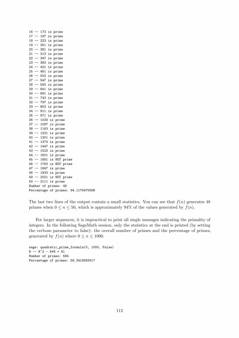
16 -- 173 is prime
17 -- 197 is prime
18 -- 223 is prime
19 -- 251 is prime
20 -- 281 is prime
21 -- 313 is prime
22 -- 347 is prime
23 -- 383 is prime
24 -- 421 is prime
25 -- 461 is prime
26 -- 503 is prime
27 -- 547 is prime
28 -- 593 is prime
29 -- 641 is prime
30 -- 691 is prime
31 -- 743 is prime
32 -- 797 is prime
33 -- 853 is prime
34 -- 911 is prime
35 -- 971 is prime
36 -- 1033 is prime
37 -- 1097 is prime
38 -- 1163 is prime
39 -- 1231 is prime
40 -- 1301 is prime
41 -- 1373 is prime
42 -- 1447 is prime
43 -- 1523 is prime
44 -- 1601 is prime
45 -- 1681 is NOT prime
46 -- 1763 is NOT prime
47 -- 1847 is prime
48 -- 1933 is prime
49 -- 2021 is NOT prime
50 -- 2111 is prime
Number of primes: 48
Percentage of primes: 94.1176470588
The last two lines of the output contain a small statistics. You can see that f(n) generates 48primes when 0 ≤ n ≤ 50, which is approximately 94% of the values generated by f(n).
For larger sequences, it is impractical to print all single messages indicating the primality ofintegers. In the following SageMath session, only the statistics at the end is printed (by settingthe verbose parameter to false): the overall number of primes and the percentage of primes,generated by f(n) where 0 ≤ n ≤ 1000.
sage: quadratic_prime_formula(0, 1000, False)
N -- N^2 - 9*N + 61
Number of primes: 584
Percentage of primes: 58.3416583417
112

Bibliography (Chap Primes)
[Blu99] Blum, W.: Die Grammatik der Logik. dtv, 1999.
[dS05] Sautoy, Marcus du: Die Musik der Primzahlen: Auf den Spuren des großten Ratselsder Mathematik. Beck, 4th edition, 2005.
[Knu98] Knuth, Donald E.: The Art of Computer Programming, vol 2: Seminumerical Algo-rithms. Addison-Wesley, 3rd edition, 1998.
[KW97] Klee, V. and S. Wagon: Ungeloste Probleme in der Zahlentheorie und der Geometrieder Ebene. Birkhauser Verlag, 1997.
[Pad96] Padberg, Friedhelm: Elementare Zahlentheorie. Spektrum Akademischer Verlag, 2nd edi-tion, 1996.
[Ric01] Richstein, J.: Verifying the Goldbach Conjecture up to 4 ∗ 1014. Mathematics ofComputation, 70:1745–1749, 2001.
[Sch96a] Schneier, Bruce: Applied Cryptography, Protocols, Algorithms, and Source Code in C.Wiley, 2nd edition, 1996.
[Sch96b] Schwenk, Jorg: Conditional Access. taschenbuch der telekom praxis. B. Seiler, VerlagSchiele und Schon, 1996.
[Sch06] Scheid, Harald: Zahlentheorie. Spektrum Akademischer Verlag, 4th edition, 2006.
[Tie73] Tietze, H.: Geloste und ungeloste mathematische Probleme. C.H. Beck, 6th edition,1973.
[WS10a] Witten, Helmut and Ralph Hardo Schulz: RSA & Co. in der Schule: Moderne Krypto-logie, alte Mathematik, raffinierte Protokolle. NF Teil 4: Gibt es genugend Primzahlenfur RSA? LOG IN, 2010(163):97–103, 2010.http://bscw.schule.de/pub/nj_bscw.cgi/d864891/RSA_u_Co_NF4.pdf.
[WS10b] Witten, Helmut and Ralph Hardo Schulz: RSA & Co. in der Schule: Moderne Krypto-logie, alte Mathematik, raffinierte Protokolle. NF Teil 5: Der Miller-Rabin-Primzahltestoder: Fallturen fur RSA mit Primzahlen aus Monte Carlo. LOG IN, 2010(166/167):92–106, 2010.http://bscw.schule.de/pub/nj_bscw.cgi/d864895/RSA_u_Co_NF5.pdf.
All links have been confirmed at July 11, 2016.
113
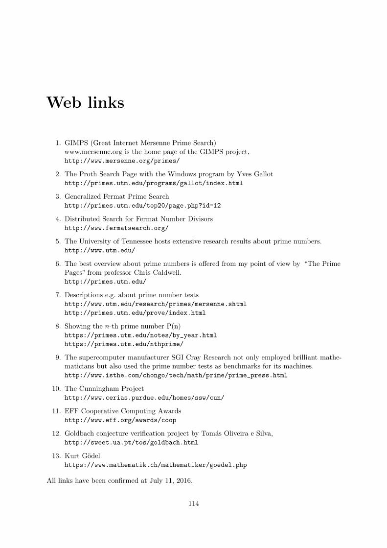
Web links
1. GIMPS (Great Internet Mersenne Prime Search)www.mersenne.org is the home page of the GIMPS project,http://www.mersenne.org/primes/
2. The Proth Search Page with the Windows program by Yves Gallothttp://primes.utm.edu/programs/gallot/index.html
3. Generalized Fermat Prime Searchhttp://primes.utm.edu/top20/page.php?id=12
4. Distributed Search for Fermat Number Divisorshttp://www.fermatsearch.org/
5. The University of Tennessee hosts extensive research results about prime numbers.http://www.utm.edu/
6. The best overview about prime numbers is offered from my point of view by “The PrimePages” from professor Chris Caldwell.http://primes.utm.edu/
7. Descriptions e.g. about prime number testshttp://www.utm.edu/research/primes/mersenne.shtml
http://primes.utm.edu/prove/index.html
8. Showing the n-th prime number P(n)https://primes.utm.edu/notes/by_year.html
https://primes.utm.edu/nthprime/
9. The supercomputer manufacturer SGI Cray Research not only employed brilliant mathe-maticians but also used the prime number tests as benchmarks for its machines.http://www.isthe.com/chongo/tech/math/prime/prime_press.html
10. The Cunningham Projecthttp://www.cerias.purdue.edu/homes/ssw/cun/
11. EFF Cooperative Computing Awardshttp://www.eff.org/awards/coop
12. Goldbach conjecture verification project by Tomas Oliveira e Silva,http://sweet.ua.pt/tos/goldbach.html
13. Kurt Godelhttps://www.mathematik.ch/mathematiker/goedel.php
All links have been confirmed at July 11, 2016.
114

Acknowledgments
I would like to take this opportunity to thank Mr. Henrik Koy and Mr. Roger Oyono for theirvery constructive proof-reading of the first versions of this article.
115

Chapter 4
Introduction to Elementary NumberTheory with Examples
(Bernhard Esslinger, Jul 2001; Updates: Dec 2001, Jun 2002, May 2003, May 2005, Mar 2006,Jun 2007, Jul 2009, Jan 2010, Aug 2013, Jul 2016)
This“introduction”is for people with a mathematical interest. There is no more pre-knowledgenecessary than what you learn in the secondary school.
We intentionally had “beginners” in mind; we did not take the approach of mathematicaltextbooks, called “introduction”, which cannot be understood at the first reading further thanpage 5 and which have the real purpose to deliver all information that special monographs canbe read.
4.1 Mathematics and cryptography
A large proportion of modern, asymmetric cryptography is based on mathematical knowledge –on the properties (“laws”) of whole numbers, which are investigated in elementary number theory.Here, the word “elementary” means that questions raised in number theory are essentially rootedin the set of natural and whole numbers.
Further mathematical disciplines currently used in cryptography include (see [Bau95, p. 2],[Bau00, p. 3]) :
• Group theory
• Combination theory
• Complexity theory
• Stochastic (ergodic theory)
• Information theory.
Number theory or arithmetic (the emphasis here is more on the aspect of performingcalculations with numbers) was established by Gauss1 as a special mathematical discipline. Its
1Carl Friedrich Gauss, German mathematician and astronomer, Apr 30, 1777−Feb 23, 1855.
116
elementary features include the greatest common divisor2 (gcd), congruence (remainder classes),factorization, the Euler-Fermat theorem and primitive roots. However, the most importantaspect is prime numbers and their multiplicative operation.
For a long time, number theory was considered to be the epitome of pure research, the idealexample of research in the ivory tower. It delved into “the mysterious laws of the realm ofnumbers”, giving rise to philosophical considerations as to whether it described elements thatexist everywhere in nature or whether it artificially constructed elements (numbers, operatorsand properties).
We now know that patterns from number theory can be found everywhere in nature. Forexample, the ratio of rotating counterclockwise and rotating clockwise spirals in a sunflower isequal to two consecutive Fibonacci numbers3, for example 21 : 34.
Also, at the latest when number theory was applied in modern cryptography, it becameclear that a discipline that had been regarded as purely theoretical for centuries actually had apractical use. Today, experts in this field are in great demand on the job market.
Applications in (computer) security now use cryptography because this mathematical disci-pline is simply better and easier to prove than all other ”creative” substitution procedures thathave been developed over the course of time and better than all sophisticated physical methodssuch as those used to print bank notes [Beu96, p. 4].
This article explains the basics of elementary number theory in a way that you can easilyunderstand. It provides numerous examples and very rarely goes into any proofs (these can befound in mathematical textbooks).
The goal is not to exhaustively explain the number theory findings, but to show the essentialprocedures. The volume of the content is so oriented that the reader can understand and applythe RSA method.
For this purpose we will use both theory and examples to explain how to perform calculationsin finite sets and describe how these techniques are applied in cryptography. Particular attentionwill be paid to the traditional Diffie-Hellman (DH) and RSA public key procedures.4
It was important to me to make verifiable statements about the security of the RSA algorithm,and to add SageMath code for as much as possible examples.
2This article deals with the gcd (greatest common divisor) in appendix 4.14.3The sequence of Fibonacci numbers (ai)i∈N is defined by the “recursive” rule a1 := a2 := 1 and for all numbersn = 1, 2, 3, · · · we define an+2 := an+1 + an. This historical sequence can be found in many interesting forms innature (for example, see [GKP94, p. 290 ff] or the website of Ron Knott, which is devoted to Fibonacci numbers).A lot is known about the Fibonacci sequence and it is used today as an important tool in mathematics.
4The same intention has the series RSA & Co. at school: New series. Links to the articles plus a short abstractcan be found at https://www.cryptoportal.org/, menu “Linksammlung”, catchword “rsa”. Unfortunately theseare currently only available in German.
117

Mathematics is the queen of sciences and number theory is the queen of mathematics.
Quote 7: Carl Friedrich Gauss
4.2 Introduction to number theory5
Number theory arose from interest in positive whole numbers 1, 2, 3, 4, · · · , also referred to asthe set of natural numbers natural numbers N. These are the first mathematical constructs usedby human civilization. According to Kronecker6, they are a creation of God. In Dedekind’s7
opinion, they are a creation of the human intellect. Dependent upon one’s ideology, this is anunsolvable contradiction or one and the same thing.
In ancient times, no distinction was made between number theory and numerology, whichattributed a mystical significance to specific numbers. In the same way as astronomy andchemistry gradually detached themselves from astrology and alchemy during the Renaissance(from the 14th century), number theory also separated itself from numerology.
Number theory has always been a source of fascination – for both amateurs and professionalmathematicians. In contrast to other areas of mathematics, many of the problems and theoremsin number theory can be understood by non-experts. On the other hand, the solutions to theseproblems or the prove to the theorems often resisted to the mathematicians for a very long time.It is therefore one thing to pose good questions but quite another matter to find the answer.One example of this is what is known as Fermat’s Last (or large) theorem.8
Up until the mid 20th century, number theory was considered to be the purest area ofmathematics, an area that had no practical use in the real world. This changed with thedevelopment of computers and digital communication, as number theory was able to provideseveral unexpected solutions to real-life tasks. At the same time, advances in informationtechnology allowed specialists in number theory to make huge progress in factorizing largenumbers, finding new prime numbers, testing (old) conjectures and solving numerical problemsthat were previously impossible to solve. Modern number theory is made up of areas such as:
• Elementary number theory
• Algebraic number theory
• Analytic number theory
• Geometric number theory
• Combinatorial number theory
• Numeric number theory
5A didactical very well prepared article about the elementary number theory can be found within the series RSA &Co. at school: Modern cryptology, old mathematics, and subtle protocols: see NF part 3 [WS08]. Unfortunatelythese are currently only available in German.
6Leopold Kronecker, German mathematician, Dec 7, 1823 − Dec 29, 18917Julius Wilhelm Richard Dedekind, German mathematician, Oct 6, 1831 − Feb 12, 1916.8One of the things we learn in mathematics at school is Pythagoras’ theorem, which states the following for aright-angle triangle: a2 + b2 = c2, where a and b are the lengths of the sides containing the right angle and c is thelength of the hypotenuse.Fermat famously proposed that an + bn 6= cn for a, b, c ∈ N and whole-number exponents n > 2. Unfortunately,the border of his book from Diophant where he made the claim did not have enough space for him to prove it.The theorem was not proven until over 300 years later [Wil95, p. 433-551].
118

• Probability theory.
All of the different areas are concerned with questions regarding whole numbers (both positiveand negative whole numbers plus zero). However, they each have different methods of dealingwith them.
This article only deals with the area of elementary number theory.
4.2.1 Convention
Unless stated otherwise:
• The letters a, b, c, d, e, k, n,m, p, q are used to present whole numbers.
• The letters i and j represent natural numbers.
• The letters p always represents a prime number.
• The sets N = {1, 2, 3, · · · } and Z = {· · · ,−3,−2,−1, 0, 1, 2, 3, · · · } are the natural andwhole numbers respectively.
119

This isn’t magic – it’s logic – a puzzle. A lot of the greatest wizards haven’t got an ounce of logic.
Quote 8: Joanne K. Rowling9
4.3 Prime numbers and the first fundamental theorem of ele-mentary number theory
Many of the problems in elementary number theory are concerned with prime numbers (seechapter 3).
Every whole number has divisors or factors. The number 1 has just one – itself, whereasthe number 12 has the six factors 1, 2, 3, 4, 6 and 12.10 Many numbers are only divisible bythemselves and by 1. When it comes to multiplication, these can be regarded as the “atoms” inthe realm of numbers.
Definition 4.3.1. Prime numbers are natural numbers greater than 1 that can only be dividedby 1 and themselves.
By definition, 1 is not a prime number.
If we write down the prime numbers in ascending order (prime number sequence), then weget:
2, 3, 5, 7, 11, 13, 17, 19, 23, 29, 31, 37, 41, 43, 47, 53, 59, 61, 67, 71, 73, 79, 83, 89, 97, · · · .
The first 100 numbers include precisely 25 prime numbers. After this, the percentage ofprimes decreases, but never reaches zero.
We come across whole numbers that are prime fairly often. In the last decade only, threeyears were prime: 1993, 1997 and 1999. If they were rare, cryptography would not be able towork with them to the extent it does.
Prime numbers can be factorized in a unique (“trivial”) way:
5 = 1 ∗ 5
17 = 1 ∗ 17
1013 = 1 ∗ 1013
1, 296, 409 = 1 ∗ 1, 296, 409.
Definition 4.3.2. Natural numbers greater than 1 that are not prime are called compositenumbers. These have at least two factors other than 1.
Examples of the decomposition (the dissection of a number into its prime factors is called
9Joanne K. Rowling, “Harry Potter and the Philosopher’s Stone”, Bloomsbury, (c) 1997, chapter “Through thetrapdoor”, p. 307, by Hermine.
10Due to the fact that 12 has so many factors, this number – and multiples of this number – is often found ineveryday life: the 12-hour scale on clocks, the 60 minutes in an hour, the 360-degree scale for measuring angles,etc. If we divide these scales into segments, the segments often turn out to be whole numbers. These are easier touse in mental arithmetic than fractions.
120
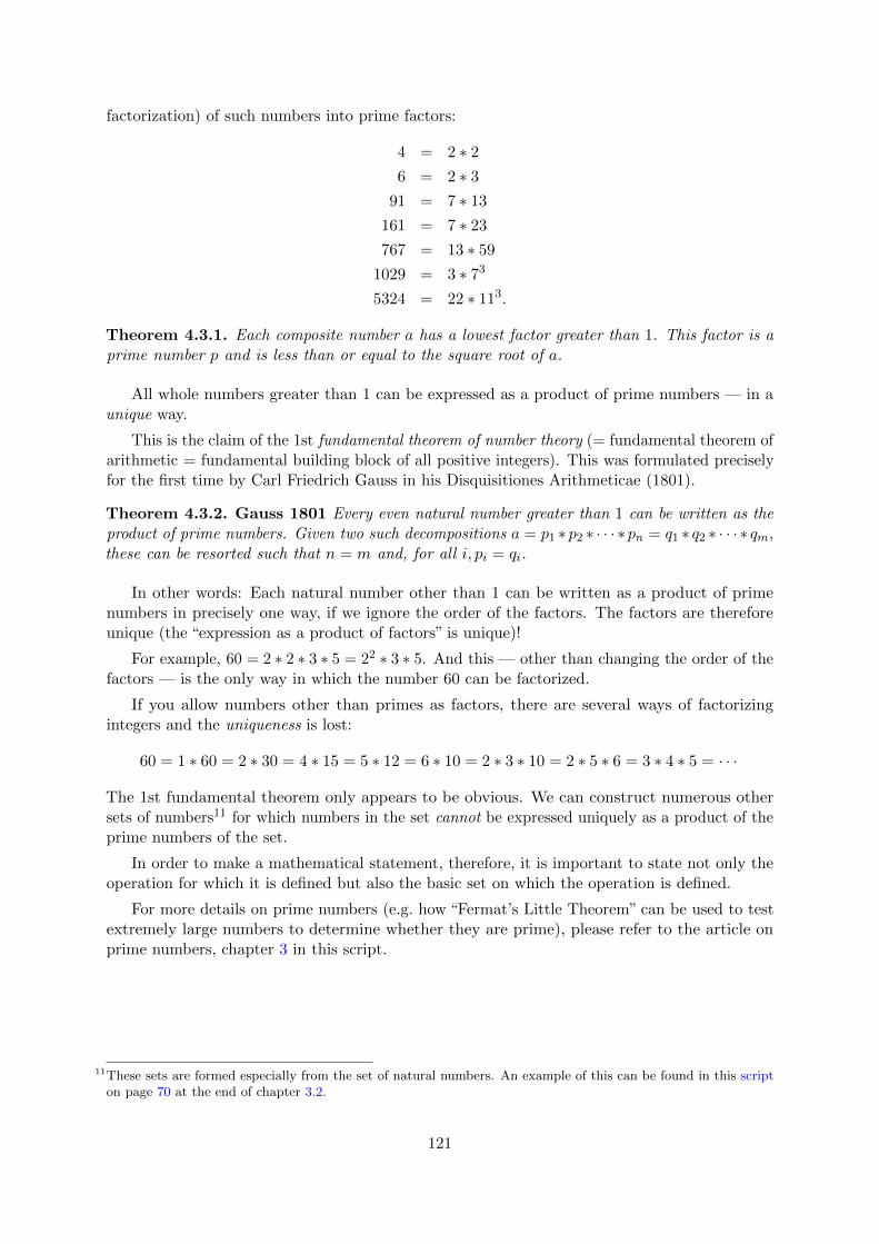
factorization) of such numbers into prime factors:
4 = 2 ∗ 2
6 = 2 ∗ 3
91 = 7 ∗ 13
161 = 7 ∗ 23
767 = 13 ∗ 59
1029 = 3 ∗ 73
5324 = 22 ∗ 113.
Theorem 4.3.1. Each composite number a has a lowest factor greater than 1. This factor is aprime number p and is less than or equal to the square root of a.
All whole numbers greater than 1 can be expressed as a product of prime numbers — in aunique way.
This is the claim of the 1st fundamental theorem of number theory (= fundamental theorem ofarithmetic = fundamental building block of all positive integers). This was formulated preciselyfor the first time by Carl Friedrich Gauss in his Disquisitiones Arithmeticae (1801).
Theorem 4.3.2. Gauss 1801 Every even natural number greater than 1 can be written as theproduct of prime numbers. Given two such decompositions a = p1 ∗ p2 ∗ · · · ∗ pn = q1 ∗ q2 ∗ · · · ∗ qm,these can be resorted such that n = m and, for all i, pi = qi.
In other words: Each natural number other than 1 can be written as a product of primenumbers in precisely one way, if we ignore the order of the factors. The factors are thereforeunique (the “expression as a product of factors” is unique)!
For example, 60 = 2 ∗ 2 ∗ 3 ∗ 5 = 22 ∗ 3 ∗ 5. And this — other than changing the order of thefactors — is the only way in which the number 60 can be factorized.
If you allow numbers other than primes as factors, there are several ways of factorizingintegers and the uniqueness is lost:
60 = 1 ∗ 60 = 2 ∗ 30 = 4 ∗ 15 = 5 ∗ 12 = 6 ∗ 10 = 2 ∗ 3 ∗ 10 = 2 ∗ 5 ∗ 6 = 3 ∗ 4 ∗ 5 = · · ·
The 1st fundamental theorem only appears to be obvious. We can construct numerous othersets of numbers11 for which numbers in the set cannot be expressed uniquely as a product of theprime numbers of the set.
In order to make a mathematical statement, therefore, it is important to state not only theoperation for which it is defined but also the basic set on which the operation is defined.
For more details on prime numbers (e.g. how “Fermat’s Little Theorem” can be used to testextremely large numbers to determine whether they are prime), please refer to the article onprime numbers, chapter 3 in this script.
11These sets are formed especially from the set of natural numbers. An example of this can be found in this scripton page 70 at the end of chapter 3.2.
121

4.4 Divisibility, modulus and remainder classes12
If whole numbers are added, subtracted or multiplied, the result is always another whole number.
The division of two whole numbers does not always result in a whole number. For example,if we divide 158 by 10 the result is the decimal number 15.8, which is not a whole number!
If, however, we divide 158 by 2 the result 79 is a whole number. In number theory we expressthis by saying that 158 is divisible by 2 but not by 10. In general, we say:
Definition 4.4.1. A whole number n is divisible by a whole number d if the quotient n/d is awhole number c such that n = c ∗ d.
n is called a multiple of d, whereas d is called a divisor or factor of n.
The mathematical notation for this is d|n (read “d divides n”). The notation d6 |n means thatd does not divide the number n.
In our example therefore: 106 |158 but 2|158.
4.4.1 The modulo operation – working with congruence
When we investigate divisibility, it is only the remainder of the division that is important. Whendividing a number n by m, we often use the following notation:
n
m= c+
r
m,
where c is a whole number and r is a number with the values 0, 1, · · · ,m− 1. This notation iscalled division with remainder, whereby c is called the whole-number “quotient” and r is the“remainder” of the division.
Example:19
7= 2 +
5
7(m = 7, c = 2, r = 5)
What do the numbers 5, 12, 19, 26, · · · have in common for division by 7? The remainder isalways r = 5. For division by 7, only the following remainders are possible:
r = 0, 1, 2, · · · , 6
If r = 0, then: m|n (“m divides n”).
The numbers that result in the same remainder r when divided by 7 are combined to formthe “remainder class r modulo 7”. Two numbers a and b belonging to the same remainder classmodulo 7 are said to be “congruent modulo 7”. Or in general:
Definition 4.4.2. The remainder class r modulo m is the set of all whole numbers a thathave the same remainder r when divided by m.
12With the educational tool for number theory NT you can have a playful view at the calculation with congruences,discussed in this and the next chapter (see NT learning unit 2.1, pages 2-9/40).NT can be called in CrypTool via the menu path Indiv. Procedures \ Number Theory Interactive \Learning Tool for Number Theory. See appendix A.6.CT2 contains a visualisation of these methods within the tutorial “World of Primes”.
122

Example of remainder classes RC:
RC 0 mod 4 = {x|x = 4 ∗ n; n ∈ Z} = {. . . ,−16,−12,−8,−4, 0, 4, 8, 12, 16, . . . }RC 3 mod 4 = {x|x = 4 ∗ n+ 3; n ∈ Z} = {. . . ,−13,−9,−5,−1, 3, 7, 11, 15, . . . }
As only the remainders 0, 1, 2, · · · ,m− 1 are possible for division modulo m, modular arithmeticworks with finite sets. For each modulo m there are precisely m remainder classes.
The result of the modulo operation can be formulated as: a mod m = a−m ∗ ba/mc
Definition 4.4.3. Two numbers a, b ∈ N are said to be congruent modulo m ∈ N if and only ifthey have the same remainder when divided by m.
We write: a ≡ b (mod m) (read a is congruent b modulo m), which means that a and bbelong to the same remainder class. The modulo is therefore the divisor. This notation wasintroduced by Gauss. Although the divisor is usually positive, a and b can also be any wholenumbers.
Example:
19 ≡ 12 (mod 7), because the remainders are equal: 19/7 = 2 remainder 5 and 12/7 = 1remainder 5.23103 ≡ 0 (mod 453), because 23103/453 = 51 remainder 0 and 0/453 = 0 remainder 0.
Theorem 4.4.1. a ≡ b (mod m) if and only if, the difference (a− b) is divisible by m, i.e. ifq ∈ Z exists with (a− b) = q ∗m.13
In other words: a ≡ b mod m ⇐⇒ m|(a− b) ⇐⇒ (a− b) ≡ 0 mod m
Therefore: If m divides the difference, there exists a whole number q such that: a = b+ q ∗m.As an alternative to the congruence notation, we can also use the divisibility notation: m|(a− b).
Example of equivalent statements:35 ≡ 11 (mod 3)⇐⇒ 35−11 ≡ 0 (mod 3), where 35−11 = 24 is divisible by 3 without remainderwhile 35 : 3 and 11 : 3 leave the remainder 2.
We can apply the above equivalence in theorem 4.4.1 if we need a quick and easy method ofdetermining whether large numbers are divisible by a certain number.
Example: Is 69, 993 divisible by 7?The number can be written in the form of a difference in which it is clear that each operand isdivisible by 7: 69, 993 = 70, 000− 7. Therefore, the difference is also divisible by 7.
Although these considerations and definitions may seem to be rather theoretical, we are sofamiliar with them in everyday life that we no longer think about the formal procedure. Forexample, the 24 hours on a clock are represented by the numbers 1, 2, · · · , 12. We obtain thehours after 12 noon as the remainder of a division by 12 and know immediately that 2 o’clock inthe afternoon is the same as 14.00.
13The above equivalence does apply only to the difference (a− b), not to the sum (a+ b)!Example:11 ≡ 2 (mod 3), therefore 11− 2 = 9 ≡ 0 (mod 3); but 11 + 2 = 13 is not divisible by 3.The statement in theorem 4.4.1 does not even apply to sums in one direction. It is correct for sums only if theremainder is 0 and only in the following direction: If a divisor divides both summands with no remainder, it alsodivides the sum with no remainder.
123

The “modular” arithmetic (based on division remainders) forms the basis of asymmetricencryption procedures. Cryptographic calculations are therefore not based on real numbers, asthe calculations you performed mostly at school, but rather on character strings with a limitedlength, in other words on positive whole numbers that cannot exceed a certain value. This is oneof the reasons why we choose a large number m and “calculate modulo m”. That is, we ignorewhole-number multiples of m and, rather than working with a number, we only work with theremainder when this number is divided by m. The result is that all results are in the range 0 tom− 1.
124

4.5 Calculations with finite sets
4.5.1 Laws of modular calculations
From algebra theorems it follows that essential parts of the conventional calculation rules arekept when we proceed to modular calculations over a basic set Z. For example, addition remainscommutative. The same goes for multiplication modulo m. The result of a division14 is not afraction but rather a whole number between 0 and m− 1.
The known laws apply:
1. Associative law:((a+ b) + c) (mod m) ≡ (a+ (b+ c)) (mod m).((a ∗ b) ∗ c) (mod m) ≡ (a ∗ (b ∗ c)) (mod m).
2. Commutative law:(a+ b) (mod m) ≡ (b+ a) (mod m).(a ∗ b) (mod m) ≡ (b ∗ a) (mod m).
The associative law and the commutative law apply to both addition and multiplication.
3. Distributive law:(a ∗ (b+ c)) (mod m) ≡ (a ∗ b+ a ∗ c) (mod m).
4. Reducibility:(a+ b) (mod m) ≡ (a (mod m) + b (mod m)) (mod m).(a ∗ b) (mod m) ≡ (a (mod m) ∗ b (mod m)) (mod m).When adding or multiplying the order in which the modulo operation is performed doesnot matter.
5. Existence of an identity (neutral element):(a+ 0) (mod m) ≡ (0 + a) (mod m) ≡ a (mod m).(a ∗ 1) (mod m) ≡ (1 ∗ a) (mod m) ≡ a (mod m).
6. Existence of an inverse element15:
– Additive inverseFor all whole numbers a and m there exists a whole number −a such that:(a+ (−a)) (mod m) ≡ 0 (mod m)
– Multiplicative inverse modulo a prime pFor each whole number a (with a 6≡ 0 (mod p) and p prime) there exists a wholenumber a−1, such that: (a ∗ a−1) (mod p) ≡ 1 (mod p)
– Multiplicative inverse modulo a compound number m16
For all whole numbers a and m (with a 6≡ 0 (mod m) and ggT (a,m) = 1) there existsa whole number a−1, such that: (a ∗ a−1) (mod m) ≡ 1 (mod m)
14The division modulo m is only defined for numbers co-prime to m because other numbers have the same propertyas zero (this means there is no inverse number). See law number 6 existence of an inverse element. Seefootnote 20 in chapter 4.6.1 and table 4.3 in chapter 4.6.2.
15An inverse element only exits, if it is unique for the given operation.16As 8 ≡ 3 mod 5 and 3 ∗ 2 ≡ 1 mod 5, then 2 = 3−1 = 8−1 is a (unique) inverse for 3 and 8.
A multiple of p or m has no inverse mod p or mod m: 5 ≡ 10 ≡ 0 mod 5.
125
7. Closeness17:a, b ∈ G =⇒ (a+ b) ∈ G.a, b ∈ G =⇒ (a ∗ b) ∈ G.
8. Transitivity:
[a ≡ b mod m, b ≡ c mod m] =⇒ [a ≡ c mod m].
4.5.2 Patterns and structures
In general mathematicians investigate “Structures”. They ask e.g. at a ∗ x ≡ b mod m, whichvalues x can take for given values of a, b, m.
Especially the case is investigated, where the result b of this operation is the neutral element.Then x is the inverse of a regarding this operation.
17The property of closeness is always defined in relation to an operation in a set. See chapter 4.15 “Appendix:Forming closed sets”.
126

The way of theory is long — it is short and effective by examples.
Quote 9: Seneca18
4.6 Examples of modular calculations
As we have already seen:
For two natural numbers a and m, a mod m denotes the remainder obtained when we dividea by m. This means that a (mod m) is always a number between 0 and m− 1.
For example, 1 ≡ 6 ≡ 41 ≡ 1 (mod 5) because the remainder is always 1. Another exampleis: 2000 ≡ 0 (mod 4) because 4 divides 2000 with no remainder.
Modular arithmetic only contains a limited quantity of non-negative numbers. The numberof these is specified by a modulus m. If the modulo is m = 5, then only the 5 numbers in the set{0, 1, 2, 3, 4} are used.
A calculation result larger than 4 is then reduced “modulo 5”. In other words, it is theremainder when the result is divided by 5. For example, 2 ∗ 4 ≡ 8 ≡ 3 (mod 5) because 3 is theremainder when we divide 8 by 5.
4.6.1 Addition and multiplication
The following shows two tables:
• the addition table19 (mod 5) (table 4.1) and
• the multiplication tables20 for mod 5 (table 4.2) and mod 6 (table 4.3).
Example of an addition table:The result when we add 3 and 4 (mod 5) is determined as follows: Calculate 3 + 4 = 7 and keepsubtracting 5 from the result until the result is less than the modulo: 7 − 5 = 2. Therefore:3 + 4 ≡ 2 (mod 5).
+ 0 1 2 3 4
0 0 1 2 3 41 1 2 3 4 02 2 3 4 0 13 3 4 0 1 24 4 0 1 2 3
Table 4.1: Addition table modulo 5
18Lucius Annaeus Seneca, philosophical writer and poet, 4 B. C. − 65 A. D.19Comment on subtraction modulo 5:
2− 4 = −2 ≡ 3 mod 5.So it is not true modulo 5 that −2 = 2 (see chapter 4.16 “Appendix: Comments on modulo subtraction”).
20Comment on modulo division:Due to the special role of zero as the identity for addition, division by zero is not permitted.For all a it is a ∗ 0 = 0, because a ∗ 0 = a ∗ (0 + 0) = a ∗ 0 + a ∗ 0. Obviously 0 has no inverse regarding themultiplication, because if there would be one, it must be 0 = 0 ∗ 0−1 = 1. Also see footnote 14 in chapter 4.5.1.
127

Example of a multiplication table:The result of the multiplication 4 ∗ 4 (mod 5) is determined as follows: Calculate 4 ∗ 4 = 16 andsubtract 5 until the result is less than the modulus.
16− 5 = 11; 11− 5 = 6; 6− 5 = 1
The table directly shows that 4 ∗ 4 ≡ 1 (mod 5) because 16 : 5 = 3 remainder 1.Remark: Multiplication is defined on the set Z excluding 0 (as 0 ∗ x is always 0, and 0 has noinverse).
* 1 2 3 4
1 1 2 3 42 2 4 1 33 3 1 4 24 4 3 2 1
Table 4.2: Multiplication table modulo 5
4.6.2 Additive and multiplicative inverses
You can use the tables to read the inverses for each number in relation to addition andmultiplication.
The inverse of a number is the number that gives the result 0 when the two numbers areadded, and 1 when they are multiplied. Thus, the inverse of 4 for addition mod 5 is 1, and theinverse of 4 for multiplication mod 5 is 4 itself, because
4 + 1 = 5 ≡ 0 (mod 5);
4 ∗ 4 = 16 ≡ 1 (mod 5).
The inverse of 1 for multiplication mod 5 is 1, while the inverse modulo 5 of 2 is 3 and, sincemultiplication is commutative, the inverse of 3 is again 2.
If we take a random number and add or multiply another number (here 4) and then add21 ormultiply the corresponding inverse (1 or 4) to the interim result (1 or 3), then the end result isthe same as the initial value.
Example:
2 + 4 ≡ 6 ≡ 1 (mod 5); 1 + 1 ≡ 2 ≡ 2 (mod 5),
2 ∗ 4 ≡ 8 ≡ 3 (mod 5); 3 ∗ 4 ≡ 12 ≡ 2 (mod 5).
In the set Z5 = {0, 1, 2, 3, 4} for the addition, and in the set Z∗5 for the multiplication, allnumbers have a unique inverse modulo 5.
In the case of modular addition, this is true for every modulo (not just for 5).
However, this is not the case for modular multiplication (important theorem):
21In general x+ y + (−y) ≡ x (mod m) [(−y) = additive inverse of y (mod m)].
128
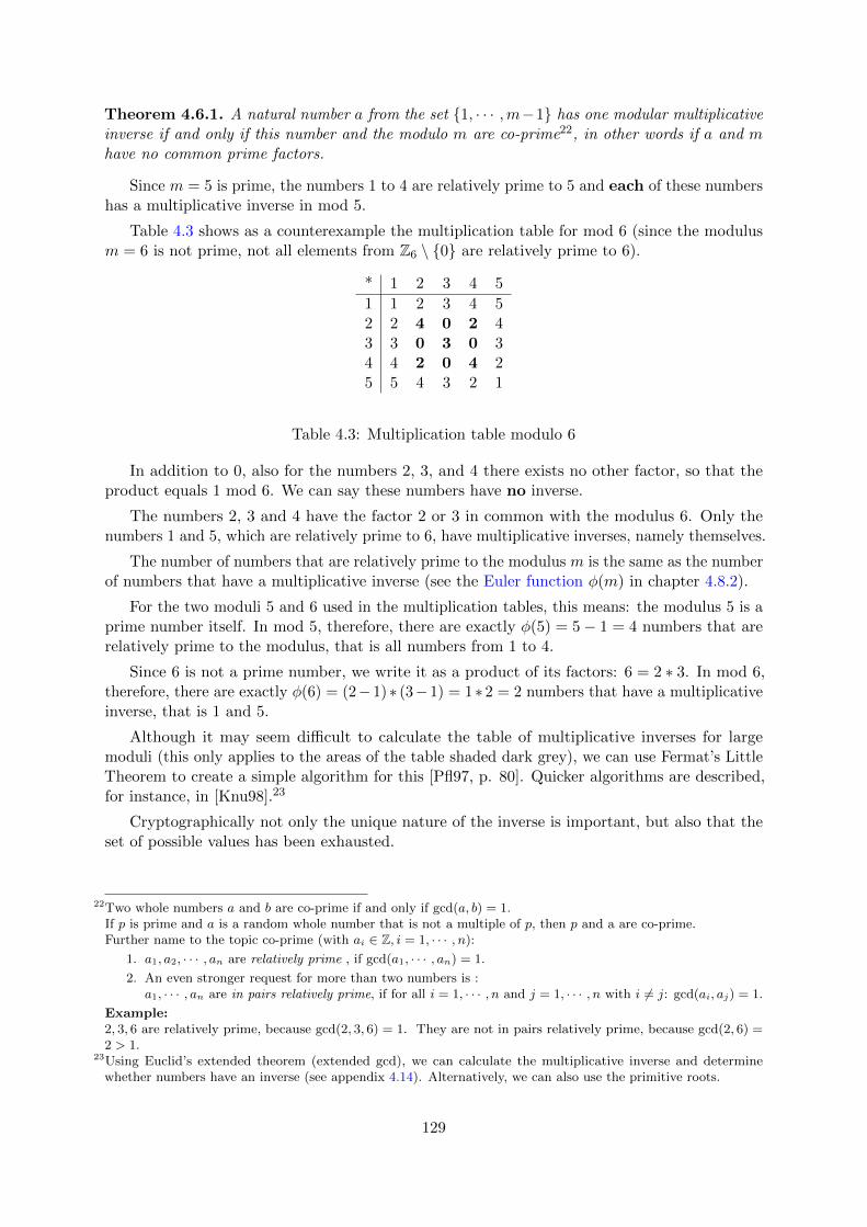
Theorem 4.6.1. A natural number a from the set {1, · · · ,m−1} has one modular multiplicativeinverse if and only if this number and the modulo m are co-prime22, in other words if a and mhave no common prime factors.
Since m = 5 is prime, the numbers 1 to 4 are relatively prime to 5 and each of these numbershas a multiplicative inverse in mod 5.
Table 4.3 shows as a counterexample the multiplication table for mod 6 (since the modulusm = 6 is not prime, not all elements from Z6 \ {0} are relatively prime to 6).
* 1 2 3 4 5
1 1 2 3 4 52 2 4 0 2 43 3 0 3 0 34 4 2 0 4 25 5 4 3 2 1
Table 4.3: Multiplication table modulo 6
In addition to 0, also for the numbers 2, 3, and 4 there exists no other factor, so that theproduct equals 1 mod 6. We can say these numbers have no inverse.
The numbers 2, 3 and 4 have the factor 2 or 3 in common with the modulus 6. Only thenumbers 1 and 5, which are relatively prime to 6, have multiplicative inverses, namely themselves.
The number of numbers that are relatively prime to the modulus m is the same as the numberof numbers that have a multiplicative inverse (see the Euler function φ(m) in chapter 4.8.2).
For the two moduli 5 and 6 used in the multiplication tables, this means: the modulus 5 is aprime number itself. In mod 5, therefore, there are exactly φ(5) = 5− 1 = 4 numbers that arerelatively prime to the modulus, that is all numbers from 1 to 4.
Since 6 is not a prime number, we write it as a product of its factors: 6 = 2 ∗ 3. In mod 6,therefore, there are exactly φ(6) = (2− 1) ∗ (3− 1) = 1 ∗ 2 = 2 numbers that have a multiplicativeinverse, that is 1 and 5.
Although it may seem difficult to calculate the table of multiplicative inverses for largemoduli (this only applies to the areas of the table shaded dark grey), we can use Fermat’s LittleTheorem to create a simple algorithm for this [Pfl97, p. 80]. Quicker algorithms are described,for instance, in [Knu98].23
Cryptographically not only the unique nature of the inverse is important, but also that theset of possible values has been exhausted.
22Two whole numbers a and b are co-prime if and only if gcd(a, b) = 1.If p is prime and a is a random whole number that is not a multiple of p, then p and a are co-prime.Further name to the topic co-prime (with ai ∈ Z, i = 1, · · · , n):
1. a1, a2, · · · , an are relatively prime , if gcd(a1, · · · , an) = 1.
2. An even stronger request for more than two numbers is :a1, · · · , an are in pairs relatively prime, if for all i = 1, · · · , n and j = 1, · · · , n with i 6= j: gcd(ai, aj) = 1.
Example:2, 3, 6 are relatively prime, because gcd(2, 3, 6) = 1. They are not in pairs relatively prime, because gcd(2, 6) =2 > 1.
23Using Euclid’s extended theorem (extended gcd), we can calculate the multiplicative inverse and determinewhether numbers have an inverse (see appendix 4.14). Alternatively, we can also use the primitive roots.
129

Theorem 4.6.2. For a, i ∈ {1, · · · ,m− 1} with gcd(a,m) = 1), then the product a ∗ i mod mtakes for a certain number a all values from {1, · · · ,m− 1} (exhaustive permutation of the lengthm− 1).24
The following three examples25 illustrate the properties of multiplicative inverses (here only thelines for the factors 5 und 6 are listed; not the complete multiplication table).
Table 4.4 (Multiplication table mod 17) was calculated for i = 1, 2, · · · , 18:
(5 ∗ i)/17 = a remainder r and high-lighted 5 ∗ i ≡ 1 (mod 17),
(6 ∗ i)/17 = a remainder r and high-lighted 6 ∗ i ≡ 1 (mod 17).
We need to find the i for which the product remainder a ∗ i modulo 17 with a = 5 or a = 6has the value 1 (i.e. the multiplicative inverse of a ∗ i).
i ⇒ 1 2 3 4 5 6 7 8 9 10 11 12 13 14 15 16 17 18
5 ∗ i 5 10 15 20 25 30 35 40 45 50 55 60 65 70 75 80 85 90remainder 5 10 15 3 8 13 1 6 11 16 4 9 14 2 7 12 0 5
6 ∗ i 6 12 18 24 30 36 42 48 54 60 66 72 78 84 90 96 102 108remainder 6 12 1 7 13 2 8 14 3 9 15 4 10 16 5 11 0 6
Table 4.4: Multiplication table modulo 17 (for a = 5 and a = 6)
Between i = 1, · · · ,m, all values between 0, · · · ,m − 1 occur for the remainders, becauseboth 5 and 6 are also relatively prime to the modulus m = 17.
The multiplicative inverse of 5 (mod 17) is 7, while the inverse of 6 (mod 17) is 3.
Table 4.5 (Multiplication table mod 13 calculates the remainders of the products 5 ∗ i and 6 ∗ i:
i ⇒ 1 2 3 4 5 6 7 8 9 10 11 12 13 14 15 16 17 18
5 ∗ i 5 10 15 20 25 30 35 40 45 50 55 60 65 70 75 80 85 90remainder 5 10 2 7 12 4 9 1 6 11 3 8 0 5 10 2 7 12
6 ∗ i 6 12 18 24 30 36 42 48 54 60 66 72 78 84 90 96 102 108remainder 6 12 5 11 4 10 3 9 2 8 1 7 0 6 12 5 11 4
Table 4.5: Multiplication table modulo 13 (for a = 5 and a = 6)
Between i = 1, · · · ,m, all values between 0, · · · ,m − 1 occur for the remainders, becauseboth 5 and 6 are relatively prime to the modulus m = 13.
The multiplicative inverse of 5 (mod 13) is 8, while the inverse of 6 (mod 13) is 11.
Table 4.6 contains an example, where the modulus m and the number a = 6 are not relativelyprime.
We have calculated (5 ∗ i) (mod 12) and (6 ∗ i) (mod 12). Between i = 1, · · · ,m, not allvalues between 0, · · · ,m− 1 occur and 6 does not have an inverse mod 12, because 6 and themodulus m = 12 are not co-prime.
24See also theorem 4.9.1 in chapter 4.9, Multiplicative order and primitive roots.25See chapter 4.19.1 “Multiplication table modulo m” for the source code to compute the tables using SageMath.130

i ⇒ 1 2 3 4 5 6 7 8 9 10 11 12 13 14 15 16 17 18
5 ∗ i 5 10 15 20 25 30 35 40 45 50 55 60 65 70 75 80 85 90remainder 5 10 3 8 1 6 11 4 9 2 7 0 5 10 3 8 1 6
6 ∗ i 6 12 18 24 30 36 42 48 54 60 66 72 78 84 90 96 102 108remainder 6 0 6 0 6 0 6 0 6 0 6 0 6 0 6 0 6 0
Table 4.6: Multiplication table modulo 12 (for a = 5 and a = 6)
The multiplicative inverse of 5 (mod 12) is 5. The number 6 has no inverse (mod12).
4.6.3 Raising to the power
In modular arithmetic, raising to the power is defined as repeated multiplication – as usual.With small exceptions we can even apply the usual rules, such as:
ab+c = ab ∗ ac,(ab)c = ab∗c = ac∗b = (ac)b
Modular powers work in the same way as modular addition and modular multiplication:
32 = 9 ≡ 4 (mod 5).
Even consecutive powers work in the same way:
Example 1:(43)2 = 642 ≡ 4096 ≡ 1 (mod 5).
(1) We can speed up26 the calculation by reducing the interim results modulo 5but we need to take care because not everything will then work in the same way asin standard arithmetic.
(43)2 ≡ (43 (mod 5))2 (mod 5)
≡ (64 (mod 5))2 (mod 5)
≡ 42 (mod 5)
≡ 16 ≡ 1 (mod 5).
(2) In standard arithmetic, consecutive powers can be reduced to a single power bymultiplying the exponents:
(43)2 = 43∗2 = 46 = 4096.
This is not quite as simple in modular arithmetic because this would give:
(43)2 ≡ 43∗2 (mod 5) ≡ 46 (mod 5) ≡ 41 ≡ 4 (mod 5).
26The time required to calculate the multiplication of two numbers normally depends on the length of the numbers.We can observe this if we use the school method to calculate, for instance, 474 ∗ 228. The time required increasesin a quadratic square manner , because we need to multiply 3 ∗ 3 numbers. The numbers become considerablysmaller if we reduce the interim result.
131

But as we saw above, the correct result is 1 !
(3) Therefore, the rule is slightly different for consecutive powers in modular arithmetic:We do not multiply the exponents in (mod m) but rather in (mod φ(m)).
Using φ(5) = 4 gives:
(43)2 ≡ 43 ∗ 2 (mod φ(5)) ≡ 46 mod 4 ≡ 42 ≡ 16 ≡ 1 (mod 5).
This delivers the correct result.
Theorem 4.6.3. (ab)c ≡ ab∗c (mod φ(m)) (mod m).
Example 2:328 = 34 ∗ 7 ≡ 34 ∗ 7 (mod 10) ≡ 38 ≡ 6561 ≡ 5 (mod 11).
4.6.4 Fast calculation of high powers
RSA encryption and decryption27 entails calculating high powers modulo m. For example, thecalculation (1005) (mod 3) exceeds the 32-bit long integer number range provided we calculate an
by actually multiplying a with itself n times in line with the definition. In the case of extremelylarge numbers, even a fast computer chip would take longer than the age of the universe tocalculate a single exponential. Luckily, there is an extremely effective shortcut for calculatingexponentials (but not for calculating logarithms).
If the expression is divided differently using the rules of modular arithmetic, then thecalculation does not even exceed the 16-bit short integer number range:
(a5) ≡ (((a2 (mod m))2 (mod m)) ∗ a) (mod m).
We can generalize this by representing the exponent as a binary number. For example, thenaive method would require 36 multiplications in order to calculate an for n = 37. However, ifwe write n in the binary representation as 100101 = 1 ∗ 25 + 1 ∗ 22 + 1 ∗ 20, then we can rewritethe expression as: a37 = a2
5+22+20 = a25 ∗ a22 ∗ a1
Example 3: 8743 (mod 103).
Since 43 = 32 + 8 + 2 + 1 , 103 is prime, 43 < φ(103)
and the squares (mod 103) can be calculated beforehand
872 ≡ 50 (mod 103),
874 ≡ 502 ≡ 28 (mod 103),
878 ≡ 282 ≡ 63 (mod 103),
8716 ≡ 632 ≡ 55 (mod 103),
8732 ≡ 552 ≡ 38 (mod 103).
27See chapter 4.10 (“Proof of the RSA procedure with Euler-Fermat”) and chapter 4.13 (“The RSA procedure withactual numbers”).
132
We have28:
8743 ≡ 8732+8+2+1 (mod 103)
≡ 8732 ∗ 878 ∗ 872 ∗ 87 (mod 103)
≡ 38 ∗ 63 ∗ 50 ∗ 87 ≡ 85 (mod 103).
The powers (a2)k can be determined easily by means of repeated squaring. As long as a doesnot change, a computer can calculate them beforehand and – if enough memory is available –save them. In order to then find an in each individual case, it now only needs to multiply those(a2)k for which there is a one in the k-th position of the binary representation of n. The typicaleffort is then reduced from 2600 to 2 ∗ 600 multiplications! This frequently used algorithm iscalled “Square and Multiply”.
4.6.5 Roots and logarithms
The inverses of the powers modulo m are also defined. The roots and logarithms are again wholenumbers. Yet in contrast to the usual situation, they are not only difficult to calculate but, inthe case of large numbers, cannot be calculated at all within a reasonable amount of time.
Let us take the equation a ≡ bc (mod m).
a) Taking the logarithm (determining c) — Discrete logarithm problem29:
If we know a and b of the three numbers a, b and c that meet this equation, then everyknown method of finding c is approximately just as time-consuming as trying out all mpossible values for c one after the other. For a typical m of the order of magnitude of10180 for 600-digit binary numbers, this is a hopeless task. More precisely, for suitablylarge numbers m, the time required according to current knowledge is proportional toexp
(C ∗ (logm[log logm]2)1/3
)with a constant C > 1.
b) Calculating the root (determining b):
The situation is similar if b is the unknown variable and we know the values of a and c:If we know the Euler function30 φ(m), then we can easily31 calculate d with c ∗ d ≡1 (mod φ(m)) and use theorem 4.6.3 to obtain:
ad ≡ (bc)d ≡ bc∗d ≡ bc∗d (mod φ(m)) ≡ b1 ≡ b (mod m)
the c-th root b of a.
If φ(m) cannot be determined32, it is difficult to calculate the c-th root. This forms thebasis for the security assumption used by the RSA encryption system (see chapter 4.10 orchapter 5.3.1).
28See chapter 4.19.2 “Fast exponentiation” for source code implementing the square and multiply method inSageMath, which can be used to reproduce the calculations above.
29Further details about the discrete logarithm problem can be found in chapter 5.4.30See chapter 4.8.2, “The Euler phi function”.31See chapter 4.14, “Appendix: gcd and the two algorithms of Euclid”.32According to the first fundamental theorem of number theory and theorem 4.8.4, we can determine φ(m) by
reducing m to prime factors.
133

The time required for inverting addition and multiplication, on the other hand, is simplyproportional to logm or (logm)2. Powers (for a number x calculate xa with a fixed) andexponents (for a number x calculate ax with a fixed) are therefore typical one way functions(compare chapters 5.1 and 4.12.1).
4.7 Groups and modular arithmetic in Zn and Z∗n
Mathematical “groups” play a decisive role in number theory and cryptography. We only talk ofgroups if, for a defined set and a defined relation (an operation such as addition or multiplication),the following properties are fulfilled:
• The set is closed
• A neutral element exists
• An inverse element exists for each element
• The associative law applies.
The abbreviated mathematical notation is (G,+) or (G, ∗).
Definition 4.7.1. Zn:
Zn comprises all numbers from 0 to n− 1 : Zn = {0, 1, 2, · · · , n− 2, n− 1}.
Zn is an often used finite group of the natural numbers. It is sometimes also called theremainder set R modulo n.
For example, 32-bit computers (standard PCs) only directly work with whole numbers in afinite set, that is the value range 0, 1, 2, · · · , 232 − 1.
This value range is equivalent to the set Z232 .
4.7.1 Addition in a group
If we define the operation mod+ on such a set where
a mod+ b := (a+ b) (mod n),
then the set Zn together with the relation mod+ is a group because the following properties of agroup are valid for all elements in Zn:
• a mod+ b is an element of Zn (the set is closed),
• (a mod+ b) mod+ c ≡ a mod+ (b mod+ c) (mod+ is associative),
• the neutral element is 0.
• each element a ∈ Zn has an inverse for this operation, namely n− a(because a mod+ (n− a) ≡ a+ (n− a) (mod n) ≡ n ≡ 0 (mod n)).
Since the operation is commutative, i.e. (a mod+ b) = (b mod+ a), this structure is actually a“commutative group”.
134
4.7.2 Multiplication in a group
If we define the operation mod* on the set Zn where
a mod∗ b := (a ∗ b) (mod n),
then Zn together with this operation is usually not a group because not all properties arefulfilled for each n.
Example:
a) In Z15, for example, the element 5 does not have an inverse. That is to say, there is no awith 5 ∗ a ≡ 1 (mod 15). Each modulo product with 5 on this set gives 5, 10 or 0.
b) In Z55 \ {0}, for example, the elements 5 and 11 do not have multiplicative inverses.That is to say, there is no a ∈ Z55 such that 5 ∗ a ≡ 1 (mod 55) and no a such that11 ∗ a ≡ 1 (mod 55). This is because 5 and 11 are not relatively prime to 55. Each moduloproduct with 5 on this set gives 5, 10, 15, . . . , 50 or 0. Each modulo product with 11 onthis set gives 11, 22, 33, 44 or 0.
On the other hand, there are subsets of Zn that form a group with the operation mod*. If wechoose all elements in Zn that are relatively prime to n, then this set forms a group with theoperation mod*. We call this set Z∗n.
Definition 4.7.2. Z∗n :Z∗n = {a ∈ Zn|gcd(a, n) = 1}.
Z∗n is sometimes also called the reduced remainder set R′ modulo n.
Example: For n = 10 = 2 ∗ 5 the following applies:
full remainder set R = Zn = {0, 1, 2, 3, 4, 5, 6, 7, 8, 9}
reduced remainder set R′ = Z∗n = {1, 3, 7, 9} −→ φ(n) = 4.
Comment:R′ or Z∗n is always a genuine subset of R or Zn because 0 is always an element of R but never anelement of R′. Since 1 and n− 1 are always relatively prime to n, they are always elements ofboth sets.
If we select a random element in Z∗n and multiply it by every other element in Z∗n, then theproducts33 are all in Z∗n, and the results are also a unique permutation of the elements in Z∗n.Since 1 is always an element of Z∗n, there is a unique “partner” in this set such that the productis 1. In other words:
Theorem 4.7.1. Each element in Z∗n has a multiplicative inverse.
Example: a = 3 modulo 10 with Z∗n = {1, 3, 7, 9} it holds that a−1 = 7:
3 ≡ 3 ∗ 1 (mod 10),
9 ≡ 3 ∗ 3 (mod 10),
1 ≡ 3 ∗ 7 (mod 10),
7 ≡ 3 ∗ 9 (mod 10).
The unique invertibility is an essential condition for cryptography (see section 4.10).
33This is due to the fact that Z∗n is closed with respect to the multiplication and due to the gcd property:[a, b ∈ Z∗n]⇒ [((a ∗ b) (mod n)) ∈ Z∗n], exactly:[a, b ∈ Z∗n]⇒ [gcd(a, n) = 1, gcd(b, n) = 1]⇒ [gcd(a ∗ b, n) = 1]⇒ [((a ∗ b) (mod n)) ∈ Z∗n].
135

Mathematical game theory postulates players who respond rationally. Transactional gametheory, on the other hand, deals with games that are not rational, perhaps even irrational and
thereby closer to reality.
Quote 10: Eric Berne34
4.8 Euler function, Fermat’s little theorem and Euler-Fermat
4.8.1 Patterns and structures
As mathematicians investigate the structure a ∗ x ≡ b mod m (see chapter 4.5.2), so they areinterested in the structure xa ≡ b mod m.
Again here they are interested in the cases, if b = 1 (value of the multiplicative inverse) and ifb = x (the function f(x) = xa mod m has a fixpoint). Concerning RSA fixed points: see 4.19.7.
4.8.2 The Euler phi function
Given n, the number of numbers from the set {1, · · · , n− 1} that are relatively prime to n isequal to the value of the Euler35 function φ(n).36
Definition 4.8.1. The Euler phi function37 φ(n) specifies the number of elements in Z∗n.
φ(n) also specifies how many whole numbers have multiplicative inverses in mod n. φ(n) canbe calculated very easily if we know the prime factors of n.
Theorem 4.8.1. For a prime number, the following is true: φ(p) = p− 1.
Theorem 4.8.2. If m is the product of two distinct primes, then:
φ(p ∗ q) = (p− 1) ∗ (q − 1) or φ(p ∗ q) = φ(p) ∗ φ(q).
This case is important for the RSA procedure.
Theorem 4.8.3. If n = p1 ∗ p2 ∗ · · · ∗ pk where p1 to pk are distinct prime numbers (i.e. nofactor occurs more than once), then the following is true (as a generalization of theorem 4.8.2):
φ(n) = (p1 − 1) ∗ (p2 − 1) ∗ · · · ∗ (pk − 1).
Theorem 4.8.4. In general, the following is true for every prime number p and every n in N:
1. φ(pn) = pn−1 ∗ (p− 1).
2. If n = pe11 ∗ pe22 ∗ · · · ∗ p
ekk , where p1 to pk are distinct prime numbers, then:
φ(n) = [(pe1−11 ) ∗ (p1− 1)] ∗ · · · ∗ [(pek−1k ) ∗ (pk− 1)] = n ∗ ([(p1− 1)/p1] ∗ · · · ∗ [(pk− 1)/pk]).
34Eric Berne, “Games People Play”, rororo, (c) 1964, page 235.35Leonhard Euler, Swiss mathematician, Apr 15, 1707 – Sep 18, 178336Also see the explanations about the Euler function φ(n) in chapter 5.3.1
”The RSA procedure“.
37The Euler phi function is also often written as Φ(n) or phi(n).
136

Example:
• n = 70 = 2 ∗ 5 ∗ 7 =⇒ using theorem 4.8.3: φ(n) = 1 · 4 · 6 = 24.
• n = 9 = 32 =⇒ using theorem 4.8.4: φ(n) = 31 · 2 = 6, because Z∗9 = {1, 2, 4, 5, 7, 8}.
• n = 2, 701, 125 = 32 ∗ 53 ∗ 74 =⇒ using theorem 4.8.4:
φ(n) = [31 ∗ 2] ∗ [52 ∗ 4] ∗ [73 ∗ 6] = 1, 234, 800.
Comment: Number-theoretic functions in CT2
The Euler phi function is just one of several number-theoretic functions or statistics used. InCT2 you can get an overview and a quick comparison for different numbers. In the followingfigure as an example the phi function for the number 24 is highlighted.
Figure 4.1: Number-theoretic functions in CT238
38Graphics from CT2, menu Crypto Tutorials, World of Primes, Distribution of primes, Number line.
137
4.8.3 The theorem of Euler-Fermat
In order to prove the RSA procedure, we need Fermat’s theorem and its generalisation (Euler-Fermat theorem) – please see chapter 3.5.
Theorem 4.8.5. Fermat’s Little Theorem39 Let p be a prime number and a be a randomwhole number, then:
ap ≡ a (mod p).
An alternative formulation of Fermat’s Little Theorem is as follows: Let p be a prime numberand a be a random whole number that is relatively prime to p, then:
ap−1 ≡ 1 (mod p).
Theorem 4.8.6. Euler-Fermat theorem (generalization of Fermat’s Little Theorem)For all elements a in the group Z∗n (i.e. a and n are natural numbers that are co-prime):
aφ(n) ≡ 1 (mod n).
This theorem states that if we raise a group element (here a) to the power of the order ofthe group (here φ(n)), we always obtain the neutral element for multiplication (the number 1).
The 2nd formulation of Fermat’s Little Theorem is derived directly from Euler’s theorem ifn is a prime number.
If n is the product of two prime numbers, we can - in certain cases - use Euler’s theorem tocalculate the result of a modular power very quickly. We have: a(p−1)∗(q−1) ≡ 1 (mod pq).
Examples for calculating a modular power:
• What is 52 (mod 6) ?With 2 = 1 ∗ 2 and 6 = 2 ∗ 3 where 2 and 3 are both prime; φ(6) = 2 because only 1 and 5are relatively prime to 6, we obtain the equation 52 ≡ 5φ(6) ≡ 1 (mod 6), without havingto calculate the power.
• What is 31792 (mod 851) ?With 792 = 22 ∗ 36 and 23 ∗ 37 = 851 where 23 and 37 are both prime, it follows for31 ∈ Z∗851 that 31792 ≡ 31φ(23∗37) ≡ 31φ(851) ≡ 1 (mod 851).
4.8.4 Calculation of the multiplicative inverse
Another interesting application is a special case of determining the multiplicative inverses usingthe Euler-Fermat theorem (multiplicative inverses are otherwise determined using the extendedEuclidean algorithm).
Example:Find the multiplicative inverse of 1579 modulo 7351.According to Euler-Fermat: aφ(n) = 1 (mod n) for all a in Z∗n. If we divide both sides by a, weget: aφ(n)−1 ≡ a−1 (mod n). For the special case that the modulo is prime, we have φ(n) = p−1.Therefore, the modular inverse is
a−1 = aφ(n)−1 ≡ a(p−1)−1 ≡ ap−2 (mod p).
For our example, this means:
39Pierre de Fermat, French mathematician, Aug 17, 1601 – Jan 12, 1665.
138

Since the modulus 7351 is prime, p− 2 = 7349.1579−1 ≡ 15797349 (mod p).
By cleverly breaking down the exponent, we can calculate this power relatively easily40:
7349 = 4096 + 2048 + 1024 + 128 + 32 + 16 + 4 + 1
1579−1 ≡ 4716 (mod 7351)
4.8.5 How many private RSA keys d are there modulo 26
According to theorem 4.6.3, the arithmetic operations of modular expressions are performed inthe exponents modulo φ(n) rather than modulo n.41
In ae∗d ≡ a1 (mod n), if we wish to determine the inverses for the factor e in the exponent,we need to calculate modulo φ(n).
Example: (with reference to the RSA algorithm)If we calculate modulo 26, which set can e and d come from?
Solution: We have e ∗ d ≡ 1 (mod φ(26)).
The reduced remainder set R′ = Z∗26 = {1, 3, 5, 7, 9, 11, 15, 17, 19, 21, 23, 25} are the elementsin Z26, which have a multiplicative inverse, that is which are relatively prime to 26 (see4.7.2).
The reduced remainder set R′′ contains only the elements of R′ that are relatively primeto φ(n) = 12 : R′′ = {1, 5, 7, 11}.
For every e in R′′ there exists a d in R′′ such that a ≡ (ae)d (mod n).
For every e in R′′, there exists therefore precisely one element (not necessarily different from e)such that e ∗ d ≡ 1 (mod φ(26)).
The general case, where n can be any integer (the sample here had n fixed to 26), is consideredin chapter 4.19.6. There is a SageMath program, calculating the number of all d. For all e thatare relatively prime to φ(n) we can calculate d as follows using the Euler-Fermat theorem:
For aφ(n) ≡ 1 (mod n) is the same as saying aφ(n)−1 ≡ a−1 (mod n). Therefore
d ≡ e−1 (mod φ(n)) ≡ eφ(φ(n))−1 (mod φ(n)).
The problems of factorizing n = pq with q 6= p and of finding φ(n) have a similar degree ofdifficulty, and if we find a solution for one of the two problems, we also have a solution for theother42 (please compare requisition 3 in section 4.10.1).
40See section 4.6.4, “Fast calculation of high powers”.41For the following example, we will adopt the usual practice for the RSA procedure of using “n” rather than “m” to
denote the modulus.42If we know the factors of n = p ∗ q with p 6= q, then φ(n) = (p− 1) ∗ (q − 1) = n− (p+ q) + 1. Additionally the
factors p and q are solutions of the quadratic equation: x2 − (p+ q)x+ pq = 0.If only n and φ(n) are known, then it is: pq = n and p+ q = n− φ(n) + 1. So you get p and q by solving theequation
x2 + (φ(n)− n− 1)x+ n = 0
139

4.9 Multiplicative order and primitive roots43
The multiplicative order and the primitive root are two useful constructs (concepts) in elementarynumber theory.
Mathematicians often ask, in which conditions the repeated application of an operationresults in the neutral element (compare Patterns and Structures, chapter 4.8.1).
For the i-times successive modular multiplication of a number a with i = 1, · · · ,m− 1 theproduct is the neutral element of the multiplication if and only if a and m are relatively prime.
Definition 4.9.1. The multiplicative order ordm(a) of a whole number a (mod m) (where aand m are co-prime) is the smallest whole number i for which ai ≡ 1 (mod m).
The following table shows that in a multiplicative group (here Z∗11) not all numbers necessarilyhave the same order. The orders in this case are 1, 2, 5 and 10 and we notice that:
1. The orders are all factors of 10.
2. The numbers a = 2, 6, 7 and 8 have the order 10 - we say that these numbers have themaximum order in Z∗11.
43With the educational tool for number theory NT you can have a playful experience with primitive roots (seelearning unit 2.2, pages 10-14/40 and 24-40/40).NT can be called in CT1 via the menu path Indiv. Procedures \ Number Theory Interactive \ LearningTool for Number Theory. See appendix A.6.Also see the SageMath samples in 4.19.3.
140

Example 1:The following table 4.744 shows the values ai mod 11 for the exponents i = 1, 2, · · · , 10, and forthe bases a = 1, 2, · · · , 10 as well as the resulting value ord11(a) for each a.
i=1 i=2 i=3 i=4 i=5 i=6 i=7 i=8 i=9 i=10 ord11(a)
a=1 1 1 1 1 1 1 1 1 1 1 1
a=2 2 4 8 5 10 9 7 3 6 1 10
a=3 3 9 5 4 1 3 9 5 4 1 5
a=4 4 5 9 3 1 4 5 9 3 1 5
a=5 5 3 4 9 1 5 3 4 9 1 5
a=6 6 3 7 9 10 5 8 4 2 1 10
a=7 7 5 2 3 10 4 6 9 8 1 10
a=8 8 9 6 4 10 3 2 5 7 1 10
a=9 9 4 3 5 1 9 4 3 5 1 5
a=10 10 1 10 1 10 1 10 1 10 1 2
Table 4.7: Values of ai mod 11, 1 ≤ a, i < 11 and according order of a mod 11
Table 4.7 shows, for example, that the order of 3 modulo 11 has the value 5.
Definition 4.9.2. If a and m are co-prime and if ordm(a) = φ(m) (i.e. a has maximum order),then we say that a is a primitive root of m.45
Not for every modulo m there is a number a, which is a primitive root. In the table 4.7, onlya = 2, 6, 7 and 8 are a primitive root with respect to mod 11 (ordm(a) = φ(11) = 10).
Using the primitive roots, we can clearly establish the conditions for which powers modulom there is a unique inverse, and where the calculations in the exponents is manageable.46
The following two tables 4.8 and 4.9 show the multiplicative orders and primitive rootsmodulo 45 and modulo 46.
44The SageMath sample 4.5 contains the source code to generate table 4.7. See chapter 4.19.3 “Multiplicative order”.45In chapter 4.19.4 “Primitive roots” there are SageMath programs to calculate primitive roots.46There is also a very good overview about primitive roots in Wikipedia: https://en.wikipedia.org/wiki/Prim
itive_root_modulo_n.
141

Example 2:The following table 4.847 shows the values ai mod 45 for the exponents i = 1, 2, · · · , 12 and forthe bases a = 1, 2, · · · , 12 as well as the resulting value ord45(a) for each a.
a \ i 1 2 3 4 5 6 7 8 9 10 11 12 ord45(a) φ(45)
1 1 1 1 1 1 1 1 1 1 1 1 1 1 24
2 2 4 8 16 32 19 38 31 17 34 23 1 12 24
3 3 9 27 36 18 9 27 36 18 9 27 36 — 24
4 4 16 19 31 34 1 4 16 19 31 34 1 6 24
5 5 25 35 40 20 10 5 25 35 40 20 10 — 24
6 6 36 36 36 36 36 36 36 36 36 36 36 — 24
7 7 4 28 16 22 19 43 31 37 34 13 1 12 24
8 8 19 17 1 8 19 17 1 8 19 17 1 4 24
9 9 36 9 36 9 36 9 36 9 36 9 36 — 24
10 10 10 10 10 10 10 10 10 10 10 10 10 — 24
11 11 31 26 16 41 1 11 31 26 16 41 1 6 24
12 12 9 18 36 27 9 18 36 27 9 18 36 — 24
Table 4.8: Values of ai mod 45, 1 ≤ a, i < 13 and according order of a mod 45
φ(45) is calculated using theorem 4.8.4: φ(45) = φ(32 ∗ 5) = 31 ∗ 2 ∗ 4 = 24.
Since 45 is not a prime, there is no “multiplicative order” for all values of a (for all numbers thatare not relatively prime to 45 : 3, 5, 6, 9, 10, 12, · · · , because 45 = 32 ∗ 5).
Example 3:Is 7 a primitive root modulo 45?
The necessary, but not sufficient requirement/condition gcd(7, 45) = 1 is fulfilled. Table 4.8shows that the number a = 7 is not a primitive root of 45, because ord45(7) = 12 6= 24 = φ(45).
47The SageMath sample 4.6 contains the source code to generate table 4.8. See chapter 4.19.3 “Multiplicative order”.
142

Example 4:The following table 4.948 answers the question as to whether the number a = 7 is a primitiveroot of 46.
The necessary, but not sufficient requirement/condition gcd(7, 46) = 1 is fulfilled.φ(46) is calculated using theorem 4.8.2: φ(46) = φ(2 ∗ 23) = 1 ∗ 22 = 22. The number 7 is aprimitive root of 46, because ord46(7) = 2 = φ(46).
a\i 1 2 3 4 5 6 7 8 9 10 11 12 13 14 15 16 17 18 19 20 21 22 23 ord
1 1 1 1 1 1 1 1 1 1 1 1 1 1 1 1 1 1 1 1 1 1 1 1 1
2 2 4 8 16 32 18 36 26 6 12 24 2 4 8 16 32 18 36 26 6 12 24 2 –
3 3 9 27 35 13 39 25 29 41 31 1 3 9 27 35 13 39 25 29 41 31 1 3 11
4 4 16 18 26 12 2 8 32 36 6 24 4 16 18 26 12 2 8 32 36 6 24 4 –
5 5 25 33 27 43 31 17 39 11 9 45 41 21 13 19 3 15 29 7 35 37 1 5 22
6 6 36 32 8 2 12 26 18 16 4 24 6 36 32 8 2 12 26 18 16 4 24 6 –
7 7 3 21 9 17 27 5 35 15 13 45 39 43 25 37 29 19 41 11 31 33 1 7 22
8 8 18 6 2 16 36 12 4 32 26 24 8 18 6 2 16 36 12 4 32 26 24 8 –
9 9 35 39 29 31 3 27 13 25 41 1 9 35 39 29 31 3 27 13 25 41 1 9 11
10 10 8 34 18 42 6 14 2 20 16 22 36 38 12 28 4 40 32 44 26 30 24 10 –
11 11 29 43 13 5 9 7 31 19 25 45 35 17 3 33 41 37 39 15 27 21 1 11 22
12 12 6 26 36 18 32 16 8 4 2 24 12 6 26 36 18 32 16 8 4 2 24 12 –
13 13 31 35 41 27 29 9 25 3 39 1 13 31 35 41 27 29 9 25 3 39 1 13 11
14 14 12 30 6 38 26 42 36 44 18 22 32 34 16 40 8 20 4 10 2 28 24 14 –
15 15 41 17 25 7 13 11 27 37 3 45 31 5 29 21 39 33 35 19 9 43 1 15 22
16 16 26 2 32 6 4 18 12 8 36 24 16 26 2 32 6 4 18 12 8 36 24 16 –
17 17 13 37 31 21 35 43 41 7 27 45 29 33 9 15 25 11 3 5 39 19 1 17 22
18 18 2 36 4 26 8 6 16 12 32 24 18 2 36 4 26 8 6 16 12 32 24 18 –
19 19 39 5 3 11 25 15 9 33 29 45 27 7 41 43 35 21 31 37 13 17 1 19 22
20 20 32 42 12 10 16 44 6 28 8 22 26 14 4 34 36 30 2 40 18 38 24 20 –
21 21 27 15 39 37 41 33 3 17 35 45 25 19 31 7 9 5 13 43 29 11 1 21 22
22 22 24 22 24 22 24 22 24 22 24 22 24 22 24 22 24 22 24 22 24 22 24 22 –
23 23 23 23 23 23 23 23 23 23 23 23 23 23 23 23 23 23 23 23 23 23 23 23 –
Table 4.9: Values of ai mod 46, 1 ≤ a, i < 24 and according order of a mod 46
Theorem 4.9.1. Given a modulus n and a number a, relative prime to n, the following holds:The set {ai (mod n)| i = 1, . . . , φ(n)} equals the multiplicative group Z∗n if and only if ordn(a) =φ(n).49,50
The multiplicative group Z∗n only contains all values from 1 to n− 1, if n is prime (see 4.7.2).
48The SageMath sample 4.7 contains the source code to generate table 4.9. See chapter 4.19.3 “Multiplicative order”.49For prime moduli p all a with 0 < a < p are of order φ(p) = p− 1. Compare table 4.8 for an example. In this
case ai(mod n) goes through all the values 1, . . . , p− 1. Exhausting all possible values of the set is an importantcryptographic proposition (compare theorem 4.6.2). This determines a permutation π(p− 1).
50Table 4.9 demonstrates that for composite moduli n not all a are of maximal order φ(n). In this example only5, 7, 11, 15, 17, 19 and 21 are of order 22.
143

Example 5: Length of cycles
The following tables 4.10 and 4.1151 serve as samples to introduce cycle lengths – this is a topicwhich goes beyond the multiplicative order.
Cycle here means a sequence of numbers ai mod n with 1 ≤ i < n for a given a, and a repeatingsequence. According to the generation method as modular power, here each number is uniquewithin a cycle. The cycles here don’t have to contain the 1 – unless this cycles belongs to amultiplicative order ≥ 1 (they have the 1 always at the end of the cycle and at the positionan−1 mod n).With l we now mean the cycle length.
The maximum cycle length lmax is φ(n).
For the following tables 4.10 and 4.11 φ(n) is (according to theorem 4.8.4):- φ(14) = φ(2 ∗ 7) = 1 ∗ 6 = 6.- φ(22) = φ(2 ∗ 11) = 1 ∗ 10 = 10.
a) If the multiplicative order exists for a, (indendently whether a is prim) it is: ordn(a) = l.Samples: The maximum length lmax
52 is achieved e.g. for:- a = 3 with lmax = ord14(a) = 6 in table 4.10, or- a = 10 with lmax = ord22(a) = 10 in table 4.11.
b) Also, if no multiplicative order exists for a, the maximum cycle length can be achieved.53
Samples:- In table 4.10: lmax = φ(14) = 6 for a = 10, 12.- In table 4.11: lmax = φ(22) = 10 for a = 2, 6, 8, 18.
51See chapter 4.19.3, “Multiplicative order” for the source code to generate the tables 4.10 und 4.11 using SageMath.
52We don’t know of a formular telling for which a the length has a maximum.53Here the sequences are built via ai mod n with 1 ≤ i < n. For composite numbers n the sequences never contain
all numbers 1, ..., n− 1.This should not be mixed up with RSA, where the “sequence” is built differently, me mod n with 0 ≤ m < n, andthis sequence then takes all numbers 0, ..., n− 1 (permutation).
144

a \ i 1 2 3 4 5 6 7 8 9 10 11 12 13 ord14(a) φ(14) l
1 1 1 1 1 1 1 1 1 1 1 1 1 1 1 6 1
2 2 4 8 2 4 8 2 4 8 2 4 8 2 0 6 3
3 3 9 13 11 5 1 3 9 13 11 5 1 3 6 6 6
4 4 2 8 4 2 8 4 2 8 4 2 8 4 0 6 3
5 5 11 13 9 3 1 5 11 13 9 3 1 5 6 6 6
6 6 8 6 8 6 8 6 8 6 8 6 8 6 0 6 2
7 7 7 7 7 7 7 7 7 7 7 7 7 7 0 6 1
8 8 8 8 8 8 8 8 8 8 8 8 8 8 0 6 1
9 9 11 1 9 11 1 9 11 1 9 11 1 9 3 6 3
10 10 2 6 4 12 8 10 2 6 4 12 8 10 0 6 6
11 11 9 1 11 9 1 11 9 1 11 9 1 11 3 6 3
12 12 4 6 2 10 8 12 4 6 2 10 8 12 0 6 6
13 13 1 13 1 13 1 13 1 13 1 13 1 13 2 6 2
14 0 0 0 0 0 0 0 0 0 0 0 0 0 0 6 1
15 1 1 1 1 1 1 1 1 1 1 1 1 1 1 6 1
16 2 4 8 2 4 8 2 4 8 2 4 8 2 0 6 3
Table 4.10: Values of ai mod 14, 1 ≤ a < 17, i < 14
145

a\i 1 2 3 4 5 6 7 8 9 10 11 12 13 14 15 16 17 18 19 20 21 ord22(a) l
1 1 1 1 1 1 1 1 1 1 1 1 1 1 1 1 1 1 1 1 1 1 1 1
2 2 4 8 16 10 20 18 14 6 12 2 4 8 16 10 20 18 14 6 12 2 0 10
3 3 9 5 15 1 3 9 5 15 1 3 9 5 15 1 3 9 5 15 1 3 5 5
4 4 16 20 14 12 4 16 20 14 12 4 16 20 14 12 4 16 20 14 12 4 0 5
5 5 3 15 9 1 5 3 15 9 1 5 3 15 9 1 5 3 15 9 1 5 5 5
6 6 14 18 20 10 16 8 4 2 12 6 14 18 20 10 16 8 4 2 12 6 0 10
7 7 5 13 3 21 15 17 9 19 1 7 5 13 3 21 15 17 9 19 1 7 10 10
8 8 20 6 4 10 14 2 16 18 12 8 20 6 4 10 14 2 16 18 12 8 0 10
9 9 15 3 5 1 9 15 3 5 1 9 15 3 5 1 9 15 3 5 1 9 5 5
10 10 12 10 12 10 12 10 12 10 12 10 12 10 12 10 12 10 12 10 12 10 0 2
11 11 11 11 11 11 11 11 11 11 11 11 11 11 11 11 11 11 11 11 11 11 0 1
12 12 12 12 12 12 12 12 12 12 12 12 12 12 12 12 12 12 12 12 12 12 0 1
13 13 15 19 5 21 9 7 3 17 1 13 15 19 5 21 9 7 3 17 1 13 10 10
14 14 20 16 4 12 14 20 16 4 12 14 20 16 4 12 14 20 16 4 12 14 0 5
15 15 5 9 3 1 15 5 9 3 1 15 5 9 3 1 15 5 9 3 1 15 5 5
16 16 14 4 20 12 16 14 4 20 12 16 14 4 20 12 16 14 4 20 12 16 0 5
17 17 3 7 9 21 5 19 15 13 1 17 3 7 9 21 5 19 15 13 1 17 10 10
18 18 16 2 14 10 4 6 20 8 12 18 16 2 14 10 4 6 20 8 12 18 0 10
19 19 9 17 15 21 3 13 5 7 1 19 9 17 15 21 3 13 5 7 1 19 10 10
20 20 4 14 16 12 20 4 14 16 12 20 4 14 16 12 20 4 14 16 12 20 0 5
21 21 1 21 1 21 1 21 1 21 1 21 1 21 1 21 1 21 1 21 1 21 2 2
22 0 0 0 0 0 0 0 0 0 0 0 0 0 0 0 0 0 0 0 0 0 0 1
23 1 1 1 1 1 1 1 1 1 1 1 1 1 1 1 1 1 1 1 1 1 1 1
24 2 4 8 16 10 20 18 14 6 12 2 4 8 16 10 20 18 14 6 12 2 0 10
25 3 9 5 15 1 3 9 5 15 1 3 9 5 15 1 3 9 5 15 1 3 5 5
Table 4.11: Values of ai mod 22, 1 ≤ a < 26, i < 22
146
4.10 Proof of the RSA procedure with Euler-Fermat
Using the Euler-Fermat theorem, we can “prove” the RSA54 procedure in the group Z∗n.
4.10.1 Basic idea of public key cryptography
The basic idea behind public key cryptography is that all participants possess a different pair ofkeys (P and S) and the public keys for all recipients are published. You can retrieve the publickey P for a recipient from a directory just as you would look up some one’s phone number in thephone book. Furthermore, each recipient has a secret key S that is needed in order to decryptthe message and that is not known to anyone else. If the sender wishes to send a message M , heencrypts it using the public key P of the recipient before sending it:
The ciphertext C is determined as C = E(P ;M), where E (encryption) is the encryptionrule. The recipient uses his private key S to decrypt the message with the decryption ruleD : M = D(S;C).
In order to ensure that this system works for every message M , the following four require-ments must be met:
1. D(S;E(P ;M)) = M for every M (invertibility) and M takes “very many” of its possiblevalues.
2. All (S, P ) pairs are different for all participants.
3. The time required to derive S from P is at least as high as the time required to decryptM with no knowledge of S.
4. Both C and M can be calculated relatively easily.
The 1st requirement is a general condition for all cryptographic encryption algorithms.
The prerequisite of the 2nd requirement can easily be met because there is a “very” largenumber of prime numbers55. In addition, that this can be ensured by a central office that issuescertificates (see chapter 4.11.5.4, S. 164).
It is this last requirement that makes the procedure actually usable. This is because it ispossible to calculate the powers in a linear amount of time (because there is a restriction on thelength of the numbers).
Although Whitfield Diffie and Martin Hellman formulated the general method as early as1976, the actual procedure that met all four requirements was only discovered later by Rivest,Shamir and Adleman.
54The RSA procedure is the most common asymmetric cryptography procedure. Developed in 1978 by RonaldRivest, Adi Shamir and Leonard Adleman, it can be used both for signatures and for encryption. Cryptographersalways associate this procedure with the abbreviation “RSA”− the following remark is meant with humor toshow that each letter combination can be used with several meanings: As country code “RSA” means the Republicof South Africa. In Britain the “Royal Society for the encouragement of Arts, Manufactures & Commerce” iscommonly known as the “RSA”.
55According to the prime number theorem (chapter 3.7.2, p. 87) of Legendre and Gauss there are approximatelyn/ ln(n) prime numbers up to the number n. This means, for example, that there are 6.5 ∗ 1074 prime numbersunder n = 2256 (= 1.1 ∗ 1077) and 3.2 ∗ 1074 prime numbers under n = 2255. Between 2255 and 2256 there aretherefore 3.3 ∗ 1074 prime numbers with precisely 256 bits. Because of this large number of primes we cannotsimply store them all – just by reasons from physics: see the number of atoms in the universe in the overviewunder 3.11.
147
4.10.2 How the RSA procedure works
The individual steps for implementing the RSA procedure can be described as follows (see [Eck14,p. 213 ff] and [Sed90, p. 338 ff]). Steps 1 to 3 constitute key generation, steps 4 and 5 are theencryption, and steps 6 and 7 are the decryption:
1. Select two distinct random prime numbers56,57 p and q and calculate n = p ∗ q.58The value n is called the RSA modulus.59
2. Select an arbitrary e ∈ {2, · · · , n− 1} such that60:e is relatively prime to φ(n) = (p− 1) ∗ (q − 1).We can then “throw away” p and q.61
3. Select d ∈ {1, · · · , n− 1} with e ∗ d ≡ 1 (mod φ(n)), i.e. d is the multiplicative inverse of emodulo φ(n).62,63 We can then “throw away” φ(n).
→ (n, e) is the public key P .
→ (n, d) is the private key S (only d must be kept secret).
4. For encryption, the message represented as a (binary) number is divided into parts suchthat each part of the number is less than n.
5. Encryption of the plaintext (or the parts of it) M ∈ {1, · · · , n− 1}:C = E((n, e);M) := M e (mod n).
6. For decryption, the ciphertext represented as a binary number is divided into parts suchthat each part of the number is less than n.
56Compaq introduced the so-called multi-prime method with high marketing effort in 2000. n was the product oftwo big and one relative small prime: n = o ∗ p ∗ q. With theorem 4.8.3 we get: φ(n) = (o− 1) ∗ (p− 1) ∗ (q − 1).This method did not assert itself.One reason probably is, that Compaq claimed a patent on it. Generally there is less understanding in Europe andwith the Open Source Initiative, that one can claim patents on algorithms. But there is really no understandingoutside the U.S., that one can get a patent for a special case (3 factors) of an algorithm (RSA), although thepatent for the general case was almost expired.JCT contains the multi-prime RSA method both within the Visuals menu of the Default Perspective as well aswithin the Algorithm Perspective.
57If the two primes p and q are equal then (me)d ≡ m mod n is not true for all m < n (although e ∗ d ≡ 1 mod φ(n)is fulfilled). Example:If n = 52 then according to theorem 4.8.4 it is φ(n) = 5 ∗ 4 = 20, e = 3, d = 7, e ∗ d = 21 ≡ 1 mod φ(n). But itis (53)7 ≡ 0 mod 25.
58The GISA (German Information Security Agency) recommends, to choose the prime factors p and q almost thesame, but not too close:
0.5 < | log2(p)− log2(q)| < 30.
They recommend to generate the primes independently and check that the restriction is fulfilled (see [BSI16]).59In CT1 und often in the literature the RSA modulo is denoted with a capital “N” .60It is recommended by cryptanalytic reasons, but not necessary to make RSA work, to select e such that:
max(p, q) < e < φ(n)− 1.61The procedure also allows us to select d freely and then calculate e. However, this has practical disadvantages.
We usually want to be able to encrypt messages “quickly”, which is why we choose a public exponent e such thatit has a short bit length compared to the modulus n and as few binary ones as possible (e.g. 216 + 1). So a fastexponentiation is possible when encrypting. We want to select the publicly known e to be an advantageous valuethat allows the exponential calculation to be performed quickly during encryption. The prime numbers 3, 17 and65537 have proved to be particularly practical for this purpose. The most often used number is 65537 = 216 + 1,or in binary: 10 · · · 0 · · · 01 (this number is prime and therefore relatively prime to many other numbers).
62For reasons of security, d should not be too small.63We start by determining either d or e depending on the implementation.
148

7. Decryption of the ciphertext (or the parts of it) C ∈ {1, · · · , n− 1}:
M = D((n, d);C) := Cd (mod n).
The numbers d, e and n are usually extremely large (e. g. d and e 300 bits, n 600 bits).
Comment:The security of the RSA algorithm depends as with all public key methods on the difficulty tocalculate the private key d from the public key (n, e).
Concretely for the RSA method does this mean:
1. It is hard to calculate φ(n) for big compounds n and
2. It is hard to calculate the prime factors of big compounds n (factorization problem).64
4.10.3 Proof of requirement 1 (invertibility)
For pairs of keys (n, e) and (n, d) that possess fixed properties in steps 1 to 3 of the RSAprocedure, the following must be true for all M < n:
M ≡ (M e)d (mod n) with (M e)d = M e∗d.
This means that the deciphering algorithm above works correctly.
We therefore need to show that:M e∗d ≡M (mod n)
We will show this in 3 steps using theorem 4.8.5 (Fermat’s Little Theorem) (according to [Beu96,p. 131ff]).
Step 1:
In the first step we show that: M e∗d ≡M (mod p)
Since n = p ∗ q and φ(p ∗ q) = (p− 1) ∗ (q − 1) and since e and d are selected in such a way thate ∗ d ≡ 1 (mod φ(n)), there is a whole number k such that: e ∗ d = 1 + k ∗ (p− 1) ∗ (q − 1).
M e∗d ≡ M1+k∗φ(n) ≡M ∗Mk∗φ(n) ≡M ∗Mk∗(p−1)∗(q−1) (mod p)
≡ M ∗ (Mp−1)k∗(q−1) (mod p) based on little Fermat : Mp−1 ≡ 1 (mod p)
≡ M ∗ (1)k∗(q−1) (mod p)
≡ M (mod p)
The requirement for using the simplified Euler-Fermat theorem (theorem 4.8.5) was that M andp are relatively prime.
Since this is not true in general, we need to consider the case when M and p are not relativelyprime. Since p is a prime number, this implies that p is a factor of M . But this means:
M ≡ 0 (mod p).
64There is no reason for the concern sometimes mentioned that there are not enough primes: Raising the dimension(exponent) of the modul always offers enough primes to consider – this is visualized in chapter 3.13 “Appendix:Visualization of the quantity of primes in higher ranges”
149

If p is a factor of M , then p is also a factor of M e∗d. Therefore:
M e∗d ≡ 0 (mod p).
Since p is a factor of both M and Me ∗ d, it is also a factor of their difference:
(M e∗d −M) ≡ 0 (mod p).
And therefore our conjecture is also true in this special case.
Step 2:
In exactly the same way we prove that: M e∗d ≡M (mod q).
Step 3:
We now combine the conjectures from step 1 and 2 for n = p ∗ q to show that:
M e∗d ≡M (mod n) for all M < n.
From step 1 and 2 we have (M e∗d −M) ≡ 0 (mod p) and (M e∗d −M) ≡ 0 (mod q). Therefore,p and q are both factors of the same number z = (M e∗d −M). Since p and q are distinct primenumbers, their product must also be a factor of this number z. Thus:
(M e∗d −M) ≡ 0 (mod p ∗ q) or M e∗d ≡M (mod p ∗ q) or M e∗d ≡M (mod n).
2
Comment 1:We can also condense the three steps if we use the theorem 4.8.6 (Euler-Fermat) – i.e. not thesimplified theorem where n = p and which corresponds to Fermat’s Little Theorem:
(M e)d ≡M e∗d ≡M (p−1)(q−1)∗k+1 ≡ ( M (p−1)(q−1)︸ ︷︷ ︸≡Mφ(n)≡1 (mod n)
)k ∗M ≡ 1k ∗M ≡M (mod n).
Comment 2:When it comes to signing messages, we perform the same operations but first use the secret keyd, followed by the public key e. The RSA procedure can also be used to create digital signatures,because:
M ≡ (Md)e (mod n).
150

4.11 Regarding the security of the RSA algorithm65
There have always been discussions about the suitability of the RSA algorithm for digitalsignatures and encryption, e. g. after publications of breakthroughs in factorization. Neverthelessthe RSA algorithm has become a de-facto standard since it was published more than 20 yearsago (compare 7.1).
The security of the RSA algorithm rests — as with all cryptographic methods — on thefollowing 4 central pillars:
• the complexity of the number theoretical problem on which the algorithm is based (herefactorization of big numbers),
• the election of fitting parameters (here the length of the module N),
• the adequate usage of the algorithm and key generation and
• the correct implementation of the algorithm.
Usage and key generation are well understood today. Implementation based on long integerarithmetic is very easy.
The following sections examine the RSA algorithm with respect to the first two points.
4.11.1 Complexity
Successful decryption or forgery of a signature — without knowing the private key — requirescalculating the e-th root mod n. The private key, this is the multiplicative inverse of e mod φ(n),can be easily determined if φ(n) is known. φ(n) again can be calculated from the prime factorsof n. Breaking of RSA therefore cannot be more difficult than factorization of the module n.
The best factorization method known today is a further development of the General NumberField Sieve (GNFS) , which was originally devised to factor only numbers of a special form(like Fermat numbers). The complexity of solving the factorization problem with the GNFS isasymptotically
O(l) = ec·(l·ln 2)1/3·(ln(l·ln(2))2/3+o(l)
Please refer to: [LL93] and [Sil00]
This formula shows, that the factorization problem belongs to the class of problems withsub-exponential time complexity (i. e. time complexity grows asymptotically not as fast as
exponential functions like el or 2l, but strictly slower, e. g. like e√l). This classification is all
that is currently known; it does not preclude the possibility that the factorization problem canbe solved in polynomial time (see 4.11.5.1).
O(l) is the average number of processor steps depending on the bit length l of the numbern to be factorized. For the best currently known factorization algorithm the constant c =(64/9)1/173 = 1923.
The inverse proposition, that the RSA algorithm can be broken only by factorization of n,is still not proven. Most number theorists consider the “RSA problem” and the factorizationproblem equivalent in terms of time complexity.
Please refer to: Handbook of Applied Cryptography [MvOV01].
65Major parts of the first part of chapter 4.11 follow the article “Vorzuge und Grenzen des RSA-Verfahrens” writtenby F. Bourseau, D. Fox, and C. Thiel [BFT02].
151

4.11.2 Security parameters because of new algorithms
Factorization algorithms66
The complexity is basically determined by the length l of the modulus n. Higher values forthis major parameter are oriented at the possibilities of the current algorithms for factorization:
• In 1994 a 129-digit RSA modulus (428 bit), published in 1977, was factorized by adistributed implementation of the Quadratic Sieve algorithm (QS), developed 1982 byPomerance. This effort took 8 months.Please refer to:
C. Pomerance: The quadratic sieve factoring algorithm [Pom84].
• In 1999 a 155-digit modulus (512 bit) was factored with an implementation of the generalnumber field sieve algorithm (GNFS), developed by Buhler, Lenstra and Pomerance. TheGNFS is more efficient than QS if n is longer than about 116 decimal digits. This efforttook 5 months.Please refer to:
J.P. Buhler, H.W. Lenstra, C. Pomerance: Factoring integers with the number fieldsieve [BLP93].
• Ten years later, end of 2009, a 232-digit modulus (768 bit) was factored by Kleinjung etc.after 2 1/2 years.Please refer to:
T. Kleinjung, et. al.: Factorization of a 768-bit RSA modulus [Kle10].
This made practically evident that a module length of 768 bit no longer prevents fromattackers.
Details about factorization progress since 1999 see chapter 4.11.4.
Lattice base reduction algorithms
The module length l is not the only parameter relevant for security. Beneath requirementsfrom implementation and engineering the sizes and the proportions of the parameters e, d and nare relevant.
65With the educational tool for number theory NT you can gather more experience with current factorizationalgorithms (see learning unit 5.1-5.5, pages 1-15/15).NT can be called in CT1 via the menu path Indiv. Procedures \ Number Theory Interactive \ LearningTool for Number Theory. See appendix A.6.The quadratic sieve (QS) can be found in CT1 and CT2; GNFS, the most modern factorization method for modulibigger than 130 decimal digits, is only part of CT2 (via YAFU and msieve).CT2 has a GeneralFactorizer component based on YAFU. This is faster than the implemented functions in CT1.So CT2 offers the following factoring methods:
- brute-force with small primes- Fermat- Shanks square forms factorization (squfof)- Pollard rho- Pollard p-1- Williams p+1- Lenstra elliptic curve method (ECM)- self-initializing quadratic sieve (SIQS)- multiple polynomial quadratic sieve (MPQS)- special number field sieve (SNFS)- general number field sieve (GNFS).
152

According attacks based on lattice reductions are a real threat for (too) simple implementa-tions of RSA. Theses attacks can be structured into the following four categories:
• Attacks against very small public keys e (e.g. e = 3).
• Attacks against relatively small private exponents d (e.g. d < n0.5).
• Factorization of the modulus n, if one of the factors p or q is partly known.
• Attacks requiring, that a part of the private key d is known.
A good overview concerning these attacks can be found in the diploma thesis of MatthiasSchneider [Sch04].
4.11.3 Forecasts about factorization of large integers
Since 1980 a lot of progress has been made. Estimations about the future development of theability to factor RSA modules vary and depend on some assumptions:
• progression in computing performance (Moore’s law: every 18 month the computing powerwill double) and in grid computing.
• development of new algorithms.
Within the last years the module bit length feasible for factorization increased — even withoutnew algorithms — by 10 bit per year. Larger numbers require not only more time to be factored,but also huge RAM storage for the solutions matrix being used by the best algorithms knowntoday. This need for storage grows like the square root of the computation time, i. e. alsosub-exponentially. Because RAM availability increased exponentially in the recent decades, itseems that this should not be the limiting factor.
An estimation of the evolution of secure key lengths was done by Lenstra/Verheul in 1999[LV01] (compare figure 7.1 in chapter 7.1).
Within the article [BFT02] Dirk Fox67 published his prognosis of an almost linear factorizationprogression, if all influencing factors are included: Each year the module length feasible forfactorization increases by 20 bit on average. So his forecast was below the more optimisticestimations of GISA and NIST.
This forecast by Dirk Fox from the year 2001 seems to prove true by the latest factorizationrecords of RSA-200 and RSA-768 (see chapter 4.11.4). His estimation for the year 2005, toachieve a bit length of 660 bit, was almost a precision landing (compare figure 4.2).
If the forecast withstands in the future then the factorization of an RSA modulus of 1024 bitcan be expected in the year 2020.
67His company Secorvo Ltd delivered a statement on the recommendation for key length selection published bythe GISA (German Information Security Agency). Chapter 2.3.1 of this statement contains a competent andunderstandable discussion of RSA security (this document exists – to my knowledge – only in German):https://www.secorvo.de/publikationen/stellungnahme-algorithmenempfehlung-020307.pdf
153

Figure 4.2: Comparison between the published factorization records (blue) and the predicteddevelopment (red) [Source Fox 2001; last addition 2011]
154

To let the possible happen, you again and again have to try the impossible.
Quote 11: Hermann Hesse68
4.11.4 Status regarding factorization of concrete large numbers
An exhaustive overview about the factoring records of composed integers using different methodscan be found on the following web pages:
http://primerecords.dk/consecutive_factorizations.htm
http://en.wikipedia.org/wiki/Integer_factorization_records
http://en.wikipedia.org/wiki/RSA_Factoring_Challenge
The current record (as of Nov. 2012) obtained using the GNFS method (general numberfield sieve) factorized a general 232 decimal digit into its both prime factors.
The last records69 with factorization algorithms for composed numbers are listed in table 4.12.
Decimal digits Binary digits Factored on Factored by
RSA-768 232 768 Dec 2010 Thorsten Kleinjung et al.RSA-200 200 663 May 2005 Jens Franke et al.
RSA-64070 193 640 Nov 2005 Jens Franke et al.RSA-576 174 576 Dec 2003 Jens Franke et al.RSA-160 160 530 Apr 2003 Jens Franke et al.RSA-155 155 512 Aug 1999 Herman te Riele et al.
. . .C307 307 1017 May 2007 Jens Franke et al.C176 176 583 May 2005 Kazumaro Aoki et al.C158 158 523 Jan 2002 Jens Franke et al.
Table 4.12: The current factoring records (as of Nov. 2012)
68Hermann Hesse, German/Swiss writer and Nobel Prize winner, July 2, 1877 − August 9, 1962.69The ’RSA numbers’ are certain large semiprime numbers (i.e., numbers with exactly two prime factors). They
were generated and published by the company RSA Security: In the RSA Factoring Challenge the prime factorsfor these numbers are sought.See http://www.emc.com/emc-plus/rsa-labs/historical/the-rsa-factoring-challenge.htm.
RSA Labs offers its challenges since the beginning of the 1990th. The first RSA Factoring Challenge labeledthe numbers, from RSA-100 to RSA-500, according to their number of decimal digits; the second RSA FactoringChallenge labeled the numbers according to their number of binary digits. Within the second challenge cashprizes were offered for successful factorizations of RSA-576 to RSA-2048 (RSA-576, RSA-640 etc. using 64 bitsteps upwards — An exception to this is RSA-617, which was created prior to the change in the numberingscheme). But the RSA challenges ended ahead of time in 2007, RSA Inc. retracted the prize. All till nowunsolved RSA challenges of RSA Labs can also be found at the website of the cipher challenge “MysteryTwisterC3” (http://www.mysterytwisterc3.org).
The ’C numbers’ originate from the Cunningham project: http://homes.cerias.purdue.edu/~ssw/cun/.These are factors of Mersenne numbers, which have a very special form. This makes it an order of magnitudeeasier to factor them as moduli of the same length build for RSA.
70A research group of the GISA solved this challenge which was awarded with 20,000 US dollar using the GNFSmethod. The researchers needed about five months to divide this number into its both 320 bit long prime factors.
The researchers around Professor Jens Franke (from the University of Bonn, the GISA, and the CWI) do notaim on getting cash prizes but in extending the research limits. So statements about the necessary length of asecure RSA modulus are more well-founded.
155

Experiences about the ellipsed time of factorization with the open source software Pari-GP,SageMath, CrypTool 1 and CrypTool 2) can be found in “Zeitexperimente zur Faktorisierung”(time experiments about factorization) (see [SW10]).
Below these last records listed in table 4.12 are explained in more detail71:
RSA-155
On August 22, 1999 researchers from the Netherlands found the solution of this RSA challenge.They factorized a 155-digit number into its both 78-digit primes (see chapter 4.11.2).
This 512 bit RSA-155 meant to reach a kind of magic border.
C158
On January 18, 2002 researchers at the German University of Bonn72 factorized a 158-digitdecimal number into its both prime factors (these are build with 73 and 86 decimal digits) usingthe GNFS method (general number field sieve).
This record got much less attention within the press than the solution of RSA-155.
The task of the researchers from Bonn was not initiated by a challenge, but they wantedto find the last prime factors of the integer 2953 − 1 (see “Wanted List” of the CunninghamProject73).
The 6 smaller prime factors, already found before have been:
3, 1907, 425796183929,1624700279478894385598779655842584377,
3802306738549441324432139091271828121 and128064886830166671444802576129115872060027.
The first 3 factors can be easily computed74. The next three prime factors were found byP. Zimmerman75, T. Grandlund and R. Harley during the years 1999 and 2000 using the ellipticcurve factorization method.
The last remaining factor, called “C158”, was known to be composite by then, but its factorswere not known (the following 3 lines contain one number):
39505874583265144526419767800614481996020776460304936454139376051579355626529450683609727842468219535093544305870490251995655335710209799226484977949442955603
The factorization of C158 resulted in the following two 73- and 86-digit prime factors:
3388495837466721394368393204672181522815830368604993048084925840555281177
71The two methods, GNFS and SNFS, used to do so are shortly illustrated at the following web pages:
http://en.wikipedia.org/wiki/Special_number_field_sieve
http://en.wikipedia.org/wiki/General_number_field_sieve72https://members.loria.fr/PZimmermann/records/gnfs15873Cunningham project: http://homes.cerias.purdue.edu/~ssw/cun/74E.g. using CT1 via menu Indiv. Procedures \ RSA Cryptosystem \ Factorization of a Number.
CT1 can factorize in a reasonable time numbers no longer than 250 bit (Numbers bigger than 1024 bits are notaccepted by CT1). CT2 is able to factorize numbers bigger than 250 bit length.
75http://homepages.loria.fr/PZimmermann/ecmnet/
156
and11658823406671259903148376558383270818131012258146392600439520994131344334162924536139.
So now all 8 prime factors of 2953 − 1 have been found.
Links:• https://members.loria.fr/PZimmermann/records/gnfs158
• https://web.archive.org/web/20170518021747/http://www.crypto-world.com:
80/announcements/c158.txt
RSA-160
On January 18, 2002 researchers at the German University of Bonn76 factorized a 160-digitnumber into its both prime factors (these are build with each 80 decimal digits) using the GNFSmethod (general number field sieve).
The computations for the factorization of RSA-160 also took place at the German InformationSecurity Agency (GISA) in Bonn.77
The 160-digit decimal number origins from the old challenge list of RSADSI. This numberwas retracted after RSA-155 (RSA512) had been factorized successfully. The prime factors ofRSA-160 were still unknown. So this record of the team of Prof. Franke provides the solution ofthe old challenge, for which RSADSI didn’t award a price anymore.
The composite number called “RSA-160” is (the following 3 lines contain one number):
215274110271888970189601520131282542925777358884567598017049767677813314521885913567301105977349105960249790711158521430
2079314665202840140619946994927570407753
The factorization of RSA-160 resulted in the following two prime factors:
p = 45427892858481394071686190649738831656137145778469793250959984709250004157335359
andq = 47388090603832016196633832303788951
973268922921040957944741354648812028493909367
The calculations took place between December 2002 and April 2003.
76https://members.loria.fr/PZimmermann/records/rsa160
https://members.loria.fr/PZimmermann/records/factor.html
https://web.archive.org/web/20170518021747/http://www.crypto-world.com:80/FactorWorld.html77Every year the GISA creates a paper to describe which crypto algorithms are feasible to generate digital signatures
according to the German signature law – under participation of experts from economy and science. To reviewsignature methods based on the factorization problem the GISA also co-operates with researchers from theUniversity of Bonn.
157

RSA-200
On May 9, 2005 the research group of Prof. Jens Franke at the German University of Bonn78
announced, that they achieved to factorize a 200-digit number into its both prime factors (theseare build with each 100 decimal digits) using the GNFS method (general number field sieve).
The composite number called “RSA-200” is (the following 3 lines contain one number):
27997833911221327870829467638722601621070446786955428537560009929326128400107609345671052955360856061822351910951365788637105954482006576775098580557613579098734950144178863178946295187237869221823983
The factorization of RSA-200 resulted in the following two prime factors:
p = 3532461934402770121272604978198464368671197400197625023649303468776121253679423200058547956528088349
andq = 79258699544783330333470858414800596877379758573642
19960734330341455767872818152135381409304740185467
The calculations took place between December 2003 and May 2005. The factorization doneby the group around Bahr, Bohm, Franke, Kleinjung, Montgomery and te Riele lasted almost 17months. The operating expense of the calculations was about 120,000 MIPS-years79.
RSA-768
On December 12, 2009 the research group around Prof. Thorsten Kleinjung80 announced,that they achieved to factorize a 232-digit number into its both prime factors (both factors have116 decimal digits). They used the GNFS method (general number field sieve) in a way wherethey did “oversieving” on several hundred computers before starting the matrix step.
The composite number called “RSA-768” is (the following 3 lines contain one number):
1230186684530117755130494958384962720772853569595334792197322452151726400507263657518745202199786469389956474942774063845925192557326303453731548268507917026122142913461670429214311602221240479274737794080665351419597459856902143413
The factorization of RSA-768 resulted in the following two prime factors (each with 384 bit):
p = 33478071698956898786044169848212690817704794983713768568912431388982883793878002287614711652531743087737814467999489
andq = 3674604366679959042824463379962795263227915816434308764267
6032283815739666511279233373417143396810270092798736308917
The calculations took about 2 1/2 years.81
78https://members.loria.fr/PZimmermann/records/rsa20079A MIPS-year (MY) is the quantity of operations a machine can perform in one year, if the machine constantly
achieves one million integer operations per second (MIPS). For illustration: a INTEL Pentium 100 processorachieves about 50 MIPS. To factorize a 2048 bit module it is estimated to need about 8.5 · 1040 MY.
80http://eprint.iacr.org/2010/006.pdf [Kle10]81This was an “academic effort” – organisations with bigger resources could do it much faster.
158

C307 / M1039
In May 2007 Prof. Franke, Prof. Kleinjung (University of Bonn), the Japanese telecom-munication company NTT and Prof. Arjen Lenstra (Polytechnical University of Lausanne)announced, that they managed to factorize a 307 digit decimal number into its both primefactors with the SNFS method (special number field sieve) within 11 months (the two factorshave 80 and 227 decimal digits).
The task of the researchers was not initiated by a challenge, but they wanted to find the lastprime factors of the Mersenne number 21039+1 (see “Wanted List” of the Cunningham Project82).
The number 21039−1 consists of 3 prime factors: The smallest one, p7 = 5080711 was alreadyknown.83
To complete this the second factor (co-divider) “C307” had to be factorized: Till then it wasonly known, that the last remaining factor was composite, but it was unknown, how many primefactors it had and what are the prime factors. The following 5 lines contain one number:
C307 = 1159420574072573064369807148876894640753899791702017724986868353538822483859966756608000609540800517947205399326123020487440286043530286191410144093453512334712739679888502263075752809379166028555105500425810771176177610094137970787973806187008437777186828680889844712
822002935201806074755451541370711023817
The factorization of C307 resulted in the following two 80- and 2276-digit prime factors:
p80 = 55853666619936291260749204658315944968646527018488637648010052346319853288374753
and
p227 = 207581819464423827645704813703594695162939708007395209881208387037927290903246793823431438841448348825340533447691122230281583276965253760914101891052419938993341097116243589620659
72167481161749004803659735573409253205425523689.
So now the number 21039 − 1 is completely factorized in its 3 prime factors.
82Cunningham project: http://homes.cerias.purdue.edu/~ssw/cun/
Cunningham table: http://homes.cerias.purdue.edu/~ssw/cun/pmain1215
The numbers in the Cunningham table have the following syntax:“(2,n)-” means 2n − 1; “(2,n)+” means 2n + 1.To describe the magnitude one writes p < n > or c < n >: “n” is the number of decimal digits and “p” and “c” tell,whether the number is prime or composite.21039 − 1 = p7 ∗ c307 = p7 ∗ p80 ∗ p227It is explained more precisely at the page of the Cunningham project:“2651+ means 2651 + 1 and the size (c209 means 209 decimal digits) of the number which was factored. Thencome the new factor(s), the discoverer and the method used. Recently, only the multiple polynomial quadraticsieve (ppmpqs), the elliptic curve method (ecm) and the number field sieve (nfs) have been used. ‘hmpqs’ standsfor hypercube multiple polynomial quadratic sieve. Under ‘new factors’, ‘p90’ means a 90-digit prime and ‘c201’ isa 201-digit composite number.”.
83This one can also be found using CT1 via menu Indiv. Procedures \ RSA Cryptosystem \ Factorizationof a Number — with the algorithms of Brent, Williams or Lenstra, which are “relatively” good to separate smallfactors. Analogously, you can do it in CT2 with the GeneralFactorizer component.
159
Links:• http://www.loria.fr/~zimmerma/records/21039-
• https://web.archive.org/web/20170518021747/http://www.crypto-world.com:
80/announcements/m1039.txt
• https://web.archive.org/web/20170518024506/http://www.crypto-world.com:
80/FactorAnnouncements.html
Size of factorized numbers compared to primality proven numbers
As you notice the factorized compound numbers built of 2 prime factors are much smallerthan the especially structured numbers, for which primality tests are able to decide whetherthese numbers are prime or not (see chapters 3.4, 3.5 and 3.6).
Length of the current world records in decimal notation:
[RSA−768 number] ←→ [49th known Mersenne prime]
232 ←→ 22, 338, 618
[see table 4.12] ←→ [see table 3.1]
4.11.5 Further research results about primes and factorization
Prime numbers are part of very many topical research areas in number theory and computerscience. Progress made with factorization is bigger than was estimated in 2005 – this is notonly due to faster computers but also new mathematical knowledge. The current status of theaccording research is discussed in chapter 10.
The security of the RSA algorithm is based on the empirical observation that factoring largenumbers is a hard problem. A module n (typically, 1024 bit) can be easily constructed as theproduct of two large primes p, q (typically, 500−600 bit each), by calculating n = pq. However,it is a hard problem to (reversely) extract p, q from n. In order to calculate the private key fromthe public key, you either need to know p and q, or the value of the Euler phi function φ(n).
Thus, any progress in efficiency of factorizing large integers will effect the security of theRSA. As a consequence, the underlying primes p, q and, thus, the module n (1024 bit as oftoday) have to be increased. In case of a quantum leap in factorization, the RSA algorithmmight be compromised.
160

4.11.5.1 Bernstein’s paper and its implication on the security of the RSA algo-rithm
In his paper “Circuits for integer factorization: a proposal”, published November 2001, D. J.Bernstein [Ber01] addresses the problem of factorizing large integers. Therefore, his results are ofrelevance from a RSA point of view. As a main result Bernstein claims that the implementationof the general number field sieve algorithm (GNFS) can be improved to factor, with the sameeffort as before, integers with three times more digits.
We note that the definition of effort is a crucial point: Bernstein claims that effort is theproduct of time and costs of the machine (including the memory used). The gist of the paperlies in the fact that he can reduce a big part of factorizing to sorting. Using Schimmler’s scheme,sorting can be optimized by massive parallel computing. At the end of section 3 Bernsteinexplains this effect: The costs of m2 parallel computers with a constant amount of memoryis a constant times m2. The costs of a computer with a single processor and memory of sizem2 is also of the order of m2, but with a different constant factor. With m2 processors inparallel, sorting of m2 numbers (with Schimmler’s scheme) can be achieved in time m, while am2-memory computer needs time of the order of m2. Decreasing memory and increasing thenumber of processors, the computing time can be reduced by a factor 1/m without additionaleffort in terms of total costs. In section 5 it is said that massive parallel computing can alsoincrease efficiency of factorizing using Lenstra’s elliptic-curve-method (a search algorithm hascosts that increase in a quadratic square manner instead of cubically).
We note that all results achieved so far are asymptotic results. This means that they onlyhold in the limit n to infinity. Unfortunately, there is no upper limit for the residual error (i.e.the difference between the real and the asymptotic value) for finite n — a problem which hasalready been addressed by the author. As a consequence, one cannot conclude whether thecosts (in the sense of Bernstein) for factorizing 1024−2048-bit RSA modules can be significantlyreduced.
There is no doubt that Bernstein’s approach is innovative. However, the reduction ofcomputing time under constant costs comes along with a massive use of parallel computing — ascenario which seems not to be realistic yet. For example, formally 1 sec computing time onone machine and 1/1,000,000 sec time parallel computing time on 1,000,000 machines mighthave same costs. In reality, it is much harder to realize the second situation, and Bernsteindoes not take into account the fixed costs, in particular for building a network between all thesecomputers.
Although distributed computing over a large network might help to overcome this problem,realistic costs for data transfer have to be taken into account — a point which was not addressedin Bernstein’s proposal.
As long as there is neither (low cost) hardware nor a distributed computing approach (basedon Bernstein’s ideas), there should not be a problem for RSA. It has to be clarified from whichmagnitude of n on Bernstein’s method could lead to a significant improvement (in the sense ofthe asymptotic result).
Arjen Lenstra, Adi Shamir et. al. analyzed the paper of Bernstein [LSTT02]. In summarythey expect a factorization improvement on how much longer the bit length of the keys could bewith a factor of 1.17 (instead of factor 3 as proposed by Bernstein).
The abstract of their paper “Analysis of Bernstein’s Factorization Circuit” says:
“... Bernstein proposed a circuit-based implementation of the matrix step of the numberfield sieve factorization algorithm. We show that under the non-standard cost function used in
161
[1], these circuits indeed offer an asymptotic improvement over other methods but to a lesserdegree than previously claimed: for a given cost, the new method can factor integers that are1.17 times larger (rather than 3.01). We also propose an improved circuit design based on a newmesh routing algorithm, and show that for factorization of 1024-bit integers the matrix step can,under an optimistic assumption about the matrix size, be completed within a day by a devicethat costs a few thousand dollars. We conclude that from a practical standpoint, the security ofRSA relies exclusively on the hardness of the relation collection step of the number field sieve.”
RSA Security concludes in its analysis of the Bernstein paper [Sec02] from April, 8 2002 also– as expected – that RSA is still not compromised.
This is still an ongoing discussion.
When this section was written (June 2002) nothing was publicly known about, how far thereexist implementations of his theoretical onsets and how much financing there was for his researchproject.
4.11.5.2 The TWIRL device
In January 2003 Adi Shamir and Eran Tromer from the Weizmann Institute of Science publisheda preliminary draft called “Factoring Large Numbers with the TWIRL Device” raising concernsabout the security of key sizes till 1024 bits [ST03a].
Their abstract summarizes their results very well: “The security of the RSA cryptosystemdepends on the difficulty in factoring large integers. The best current factoring algorithm isthe Number Field Sieve (NFS), and its most difficult part is the sieving step. In 1999 a largedistributed computation involving thousands of workstations working for many months managedto factor a 512-bit RSA key, but 1024-bit keys were believed to be safe for the next 15-20 years.In this paper we describe a new hardware implementation of the NFS sieving step ... which is 3-4orders of magnitude more cost effective than the best previously published designs ... . Basedon a detailed analysis of all the critical components (but without an actual implementation), webelieve that the NFS sieving step for 1024-bit RSA keys can be completed in less than a yearwith a $10M device, and that the NFS sieving step for 512-bit RSA keys can be completed inless than ten minutes with a $10K device. Coupled with recent results about the difficulty ofthe NFS matrix step ... this raises some concerns about the security of these key sizes.”
A detailed explanation from these two authors also can be found in the RSA LaboratoriesCryptoBytes [ST03b].
The 3-page article in the DuD issue of June 2003 [WLB03] contains a very good explanation,how the attack using the generalized number field sieve (GNFS) works and which progressis made, to factorize numbers. At GNFS we can distinguish 2 general steps: The sieve step(relation collecting) and the matrix reduction. Besides the sieve step is highly parallelizable, itdominates the overall calculation burden. Shamir and Tromer haven’t built a TWIRL deviceyet, but the estimated costs of 10 till 50 million Euro (in order to factorize a 1024-bit number)is not prohibitive for secret agencies or big criminal organizations, because the “costs for a singleespionage satellite is estimated e.g. to be several billion USD”. The authors therefore recommend,to get as soon as possible rid of today used sensible RSA, Diffie-Hellman or ElGamal keys upto 1024 bit and to use then keys of at least 2048 bit length. The planned TCPA/Palladiumhardware will use 2048-bit RSA keys!
So recommendations like the ones from the GISA (German Information Security Agency) touse higher key lengths are very valid.
162

4.11.5.3 “Primes in P”: Primality testing is polynomial
In August 2002 the three Indian researchers M. Agrawal, N. Kayal and N. Saxena publishedthe paper “PRIMES in P” about a new primality testing algorithm called AKS [AKS02]. Theydiscovered a polynomial time deterministic algorithm for determining if a number is prime ornot.
The importance of this discovery is that it provides number theorists with new insightsand opportunities for further research. Lots of people over centuries have been looking for apolynomial time test for primality, and this result is a major theoretic breakthrough. It showsthat new results can be generated from already known facts.
But even its authors note that other known algorithms may be faster (for example ECPP).The new algorithm works on any integer. For example the GIMPS project uses the Lucas-Lehmerprimality test which takes advantage of the special properties of Mersenne numbers. This makesthe Lucas-Lehmer test much faster, allowing to test numbers with millions of digits while generalpurpose algorithms are limited to numbers with a few thousand digits.
Current research results on this topic can be found at:
http://www.mersenne.org/
http://fatphil.org/maths/AKS/ Original paper in Englishhttp://ls2-www.cs.uni-dortmund.de/lehre/winter200203/kt/material/primes.ps
Good explanation in German by Thomas Hofmeister.
163
4.11.5.4 Shared Primes: Modules with common prime factors
The RSA algorithm is based on the presumed difficulty of factoring large bi-prime integers(moduli), the factoring problem. However, as pointed out in Lenstra et al [LHA+12] it is possible,given a set of moduli, to factor some of them if they share primes. In this case, the factoringproblem is bypassed using the – relatively easy greatest common divisor (gcd) operation. On theother hand, it is no trivial task to extract common shared primes and to factor the accordingmoduli efficiently for a very big number of given moduli (several millions).
Using the gcd only works if the RSA keys were not generated randomly. Taking intoconsideration the significance of strong cryptographic keys it is important to verify that all keyswere generated following the principle of true randomness [ESS12].
When Lenstra et al published their paper [LHA+12] in Feb 2012, they did not publish thesource code. However, soon afterwards the source code of a similar program was published atthe CrypTool website84 in Python and C++, and – again a bit later – at the page used by[HDWH12]85. The fastest code known to me comes with [HDWH12].
These applications find all shared factors that may exist, given a finite set of moduli – evenif this set includes millions of moduli. Such an application enables system administrators to testtheir own RSA keys.
The quite naive way to find all shared factors would be to compare each modul with all othermoduli which has a complexity growing quadratically with the number of moduli.
A very efficient method using trees for comparing all gcd pairs is based on a publication ofDan Bernstein in 2005 [Ber05]. Bernstein uses a precalculation which leads to the product of allmoduli. It’s another example showing how helpful precalculations can be to break cryptographicsystems (another famous example are rainbow tables used to find the origin of a hash value[Oec03]).
The following SageMath sample shows the very different run times when calculating a gcdand a factorization. The section after this sample will explain the essential part of the methodused in [HDWH12]: Using two trees accelerates the calculation of the gcd pairs a lot.
The SageMath sample 4.1 shows that multiplication of factors, dividing a modul with aknown factor, or calculating the gcd is very fast. However, factoring moduli steeply increaseswith longer moduli. Even the relatively small moduli used in this example show this: The smallermodul (69 decimal digits, 228 bit) took 76 seconds, while the bigger one (72 decimal digits, 239bit) took almost 217 seconds.
In addition, the operations multiplication, divsion and gcd show big differences in runtimewhen the used operands are very different in size.
84http://www.cryptool.org/en/ctp-dokumentation-en/361-ctp-paper-rsa-moduli85https://www.factorable.net/
164

SageMath sample 4.1 Comparing the runtime of calculating a gcd and performing a factor-ization
# Multiplication
sage: 3593875704495823757388199894268773153439 * 84115747449047881488635567801
302301541122639745170382530168903859625492057067780948293331060817639
sage: 3593875704495823757388199894268773153439 * 162259276829213363391578010288127
583139672825572068433667900695808357466165186436234672858047078770918753
# Division
sage: time 302301541122639745170382530168903859625492057067780948293331060817639 /
3593875704495823757388199894268773153439
Wall time: 0.00 s
84115747449047881488635567801
sage: time 583139672825572068433667900695808357466165186436234672858047078770918753 /
3593875704495823757388199894268773153439
Wall time: 0.00 s
162259276829213363391578010288127
# Calculate gcd
sage: time gcd (583139672825572068433667900695808357466165186436234672858047078770918753,
302301541122639745170382530168903859625492057067780948293331060817639)
Wall time: 0.00 s
3593875704495823757388199894268773153439
# Factorize
sage: time factor (583139672825572068433667900695808357466165186436234672858047078770918753)
Wall time: 217.08 s
162259276829213363391578010288127 * 3593875704495823757388199894268773153439
sage: time factor (302301541122639745170382530168903859625492057067780948293331060817639)
Wall time: 76.85 s
84115747449047881488635567801 * 3593875704495823757388199894268773153439
165

Efficient computing of all gcd pairs and explanation of the for-mula used to determine the shared primes
The excellent paper “Mining Your Ps and Qs: Detection of Widespread Weak Keys in NetworkDevices” [HDWH12] explains the algorithm how the gcd’s of every pair of RSA moduli arecalculated efficiently.
First the product P of all moduli mi is calculated using a product tree. Then a remaindertree is build modulo the squares of the moduli. Then the gcd’s of a defined modul mi and of theremainders zi divided by this defined modul are calculated.
This is visualized in Figure 4.3 which is a copy from [HDWH12] (where the moduli are calledNi instead of mi):
Figure 4.3: Algorithm and figure to compute all gcd pairs efficiently
The paper [HDWH12] explains well how the algorithm works, but not as well why. Theproduct P of all moduli is a very big number, even compared to a single modul. Withoutthe simplifications from the remainder tree you would go the following way: Calculate gcdi =gcd(P/mi,mi) for all i. Compare each gcdi 6= 1 with all other gcdj 6= 1 with j 6= i. If two gcd’sare the same, then their moduli share a factor.86
As it’s very slow to calculate this for numbers with such a big difference in size, the remainder
86A prerequisite for getting only prime factors, is that duplicate moduli are removed before setting up the trees.
166

tree is used. Despite it seems to consist of more steps it’s a huge simplification.
Within the remainder tree you get – at the end – (P mod (m2i ))/mi for all i.87
The main remaining question now is: Why does gcd((P mod m2i )/mi,mi) deliver the same
result as gcd(P/mi,mi)? We prove that this identity is correct.88
gcd((P mod m2i )/mi,mi)
!= gcd(P/mi,mi)
⇐⇒ 89
gcd(((P mod m2i )/mi) mod mi,mi)
!= gcd((P/mi) mod mi,mi)
⇐⇒ 90
((P mod m2i )/mi) mod mi
!= (P/mi) mod mi
⇐⇒ 91
(P mod m2i )/mi − P/mi ≡ 0 mod mi ⇔ mi | ((P mod m2
i )/mi − P/mi)
92
mi | ((P −m2i ∗ bP/m2
i c − P ))/mi
93
mi | (mi ∗ bP/m2i c)
As this is true, we can conclude that the two gcds are equivalent.
87It would not make sense to calculate modulo mi instead of m2i on the left gcd, which would mean to use
(P mod mi)/mi, as mi|P , so P/mi is always a whole number, which means (P mod mi) is always = 0.Sample with very small moduli:m1 = 2 ∗ 3 = 6; m2 = 2 ∗ 7 = 14; P = 6 ∗ 14 = 84P mod m1 = 84 mod 6 = 0; P mod m2
1 = 84 mod 36 = 12P mod m2 = 84 mod 14 = 0; P mod m2
2 = 84 mod 196 = 84gcd1 = gcd(12/6, 6) = gcd(2, 6) = 2gcd2 = gcd(84/14, 14) = gcd(6, 14) = 2
The way the tree is structured it also would not make sense to first divide and then do the modulo calculation,as making the division first would lead just to the given moduli but in reversed order.
It also would not make sense to calculate (P mod (m3i ))/m
2i ) as this is only additional effort with no improvement.
88P represents here the product of all moduli, and mi represents any arbitrary modulus.89According to Euklid’s algorithm (first iteration) the following identity is true:gcd(a, b) = gcd(b, a mod b) if b 6= 0This holds as per definition it is: gcd(a, 0) = aApplied to our problem this means:gcd((P mod m2
i )/mi,mi) = gcd((P mod m2i )/mi mod mi,mi)
gcd(P/mi,mi) = gcd(P/mi mod mi,mi)90The gcd’s are equal if both their first arguments are equal.91The following transformations are all equalities.92Using the modulus operation (definition 4.4.2 at page 122) and division it is: a mod b = a− b ∗ ba/bc
So P mod m2i can be written as P −m2
i bP/m2i c.
93P reduces itself, the exponent in the mi enumerator is simplified with the mi denominator.
167
It is our choices, that show what we truly are, far more than our abilities.
Quote 12: Joanne K. Rowling94
4.12 Applications of asymmetric cryptography using numericalexamples
The results of modular arithmetic are used extensively in modern cryptography. Here we willprovide a few examples from cryptography using small95 numbers.96
Enciphering a text entails applying a function (mathematical operation) to a character string(number) to generate a different number. Deciphering entails reversing this function, in otherwords using the distorted image that the function has created from the plaintext in order torestore the original image. For example, the sender could take the plaintext M of a confidentialmessage and add a secret number, the key S, to obtain the ciphertext C:
C = M + S.
The recipient can reconstruct the plaintext by reversing this operation, in other words bysubtracting S:
M = C − S.Adding S reliably makes the plaintext impossible to read. However, this encryption is ratherweak, because all an interceptor needs to do to calculate the key is to obtain a plaintext and theassociated ciphertext
S = C −M,
and can then read any subsequent messages encrypted using S.The essential reason for this is that subtraction is just as simple an operation as addition.
4.12.1 One-way functions
If the key is to be impossible to determine even with knowledge of both the plaintext and theciphertext, we need a function that is, on the one hand, relatively easy to calculate – we don’twant to have problems encrypting messages. On the other hand, the inverse function should exist(otherwise information would be lost during encryption), but should be de facto incalculable.
What are possible candidates for such a one way function? We could take multiplicationrather than addition, but even primary school children know that the inverse function, division,is only slightly more difficult than multiplication itself. We need to go one step higher in thehierarchy of calculation methods. It is still relatively simple to calculate the power of a number,but the corresponding two reverse functions – taking roots (find b in the equation a = bc whena and c are known) and calculating logarithms (find c in the above equation when a and b areknown) are so complicated that pupils normally do not learn them at school.
94Joanne K. Rowling, “Harry Potter and the Chamber of Secrets”, Bloomsbury, 1998, last chapter “Dobby’s reward”,p. 245, by Dumbledore.
95In the RSA procedure, we call numbers “small” if the bit lengths are much less than 1024 bits (i.e. 308 decimalpoints). In practice, 1024 bits is currently considered the minimum length for a secure RSA modul.
96Within the series RSA & Co. at school: Modern cryptology, old mathematics, and subtle protocols there aredidactically very well prepared articles with code samples in Python and SageMath. Unfortunately these arecurrently only available in German. See for instance [WSE15].
168
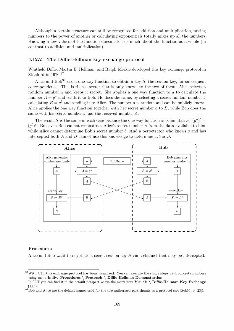
Although a certain structure can still be recognised for addition and multiplication, raisingnumbers to the power of another or calculating exponentials totally mixes up all the numbers.Knowing a few values of the function doesn’t tell us much about the function as a whole (incontrast to addition and multiplication).
4.12.2 The Diffie-Hellman key exchange protocol
Whitfield Diffie, Martin E. Hellman, and Ralph Merkle developed this key exchange protocol inStanford in 1976.97
Alice and Bob98 use a one way function to obtain a key S, the session key, for subsequentcorrespondence. This is then a secret that is only known to the two of them. Alice selects arandom number a and keeps it secret. She applies a one way function to a to calculate thenumber A = ga and sends it to Bob. He does the same, by selecting a secret random number b,calculating B = gb and sending it to Alice. The number g is random and can be publicly known.Alice applies the one way function together with her secret number a to B, while Bob does thesame with his secret number b and the received number A.
The result S is the same in each case because the one way function is commutative: (ga)b =(gb)a. But even Bob cannot reconstruct Alice’s secret number a from the data available to him,while Alice cannot determine Bob’s secret number b. And a perpetrator who knows g and hasintercepted both A and B cannot use this knowledge to determine a, b or S.
�
�
? ?
�-
PPPPPPPPPPPPPPq
��������������)? ?
� -
?
?
?
?
? ?
� -
�
�Alice Bob
a b
gg
A = ga B = gb
A
A
B
B S := AbS := Ba
S S
Public: g
Alice generates Bob generates
number randomly number randomly
secret key secret key
Procedure:
Alice and Bob want to negotiate a secret session key S via a channel that may be intercepted.
97With CT1 this exchange protocol has been visualized: You can execute the single steps with concrete numbersusing menu Indiv. Procedures \ Protocols \ Diffie-Hellman Demonstration.In JCT you can find it in the default perspective via the menu item Visuals \ Diffie-Hellman Key Exchange(EC).
98Bob and Alice are the default names used for the two authorized participants in a protocol (see [Sch96, p. 23]).
169

1. They select a prime number p and a random number g and exchange this informationopenly.
2. Alice now selects a, a random number less than p and keeps it secret.
Similarly, Bob selects b, a random number less than p and keeps it secret.
3. Alice now calculates A ≡ ga (mod p).Bob calculates B ≡ gb (mod p).
4. Alice sends the result A to Bob.Bob sends the result B to Alice.
5. In order to now determine the session key to be used by both, they both separately raisethe respective results they have received to the power of their secret random numbermodulo p. This means:
- Alice calculates S ≡ Ba (mod p) and
- Bob calculates S ≡ Ab (mod p).
Even if a spy intercepts g, p, and the interim results A and B, he cannot use these in order todetermine the session key used – due to the difficulty of calculating the discrete logarithm99.
We will now use an example with (unrealistically) small numbers to illustrate this.
Example using small numbers:
1. Alice and Bob select g = 11, p = 347.
2. Alice selects a = 240, Bob selects b = 39 and they keep a and b secret.
3. Alice calculates A ≡ ga ≡ 11240 ≡ 49 (mod 347).Bob calculates B ≡ gb ≡ 1139 ≡ 285 (mod 347).
4. Alice sends Bob: A ≡ 49,Bob sends Alice: B ≡ 285.
5. Alice calculates Ba ≡ 285240 ≡ 268 (mod 347),Bob calculates Ab ≡ 4939 ≡ 268 (mod 347).
Alice and Bob can now communicate securely using their shared session key S. Even if spiescould intercept everything transferred via the connection g = 11, p = 347, A = 49, and B = 285;they would not be able to calculate the secret key S.
However, this is only true for large numbers because then the discrete logarithm is extremelydifficult to solve (see chapter 10).
99Further details about the discrete logarithm problem can be found in chapters 5.4 and 10.
170

Comment:
For such small numbers as in the example above, the DH key exchange scheme can be attackedas the discrete logarithms can be easily calculated in order to reveal the exponents a or b.
After revealing a or b, S can be calculated in the same way as Alice or Bob do it.
To get the discrete logarithms, here we need to calculate one of the following equations:
a from Alice: 11x ≡ 49 (mod 347), that means log11(49) (mod 347).
b from Bob: 11y ≡ 285 (mod 347), that means log11(285) (mod 347).
You can use SageMath to determine the discrete logarithm x that solves for instance the equationabove (i.g. for Alice):
SageMath sample 4.2 Sample with small numbers: calculating the discrete logs a and b inorder to attack DH# Get the secret key of Alice:
### via numbers
sage: discrete_log(mod(49,347),mod(11,347))
67
### via variables in the ring of integers
sage: R=Integers(347)
sage: g=R(11)
sage: A=R(49)
sage: discrete_log(A,g)
67
# Get the secret key of Bob:
sage: B=R(285)
sage: discrete_log(B,g)
39
As the SageMath function discrete log expects as arguments only elements of a ring (integersbetween 0 and an upper limit), we could either enforce this type by entering the numbers directlywith the according modulo operator: discrete_log(mod(49, 347), mod(11, 347)).A much better alternative is to use the variables like in the formula above and let SageMathknow that they are elements of a ring. After this “burdon” at the beginning for the initialization,you can write the formulars like you are used to: discrete_log(A, g).100,101
100Such number theoretic tasks can also be solved using other tools like PariGP, LiDIA, BC, or Mathematica (seethe list of web sites in the appendix at the end of this chapter). Here is the according syntax to get the discretelog for Alice:• Pari-GP: znlog(Mod(49,347),Mod(11,347))• LiDIA: dl(11,49,347)• Mathematica: MultiplicativeOrder[11, 347, 49]
The general “Solve” function provides the “em tdep message”: The equations appear to involve the variablesto be solved for in an essentially non-algebraic way.
All function calls deliver the result 67.101Why have the functions delivered the value 67 for the discrete logarithm of Alice rather than 240 which Alice
selected as exponent a?The discrete logarithm is the smallest natural exponent that solves the equation 11x ≡ 49 (mod 347). Both x = 67and x = 240 (the number selected in the example) satisfy the equation and can therefore be used to calculate thesession key: 285240 ≡ 28567 ≡ 268 (mod 347). If Alice and Bob had selected a primitive root modulo p as base g,then for every remainder from the set {1, 2, . . . , p− 1} there is exactly one exponent from the set {0, 1, . . . , p− 2}.
As an aside, there are 172 different primitive roots modulo 347, 32 of which are prime (not necessary). Sincethe number 11 selected for g in the example is not a primitive root of 347, the remainders do not take all valuesfrom the set {1, 2, . . . , 346}. Thus, for a particular remainder there may be more than one exponent or even noexponent at all in the set {0, 1, . . . , 345} that satisfies the equation.
171

4.13 The RSA procedure with actual numbers102
“Games are Nature’s way of preparing us to face difficult realities. Are you finally ready to facereality, Sergeant?”
Quote 13: Daniel Suarez103
Having described above how the RSA procedure works, we will now work through the stepsusing actual, but small, numbers.
4.13.1 RSA with small prime numbers and with a number as message
Before applying the RSA procedure to a text, we will first demonstrate it directly using a singlenumber104 as message.105
1. Let the selected prime numbers be p = 5 and q = 11.Thus, n = 55 and φ(n) = (p− 1) ∗ (q − 1) = 40.
2. e = 7 (e should106 lie between 11 and 39, and must be relatively prime to 40).
3. d = 23 (since 23 ∗ 7 ≡ 161 ≡ 1 (mod 40)),
→ Public key of the recipient: (55, 7),
→ Private key of the recipient: (55, 23).
4. Let the message be the number M = 2 (so no division into blocks is required).
5. Encryption: C ≡ 27 ≡ 18 (mod 55).
6. The ciphertext is simply the number C = 18 (we therefore do not need to divide it intoblocks).
7. Decryption: M ≡ 1823 ≡ 18(1+2+4+16) ≡ 18 ∗ 49 ∗ 36 ∗ 26 ≡ 2 (mod 55).
With the relevant SageMath commands you find:is_prime(347)=True, euler_phi(347)=346, gcd(11,347)=1, and multiplicative_order(mod(11, 347))=173.
i 11i mod 347
0 11 112 1213 29067 49 searched exponent172 284173 1 = multiplicative order of 11i mod 347174 11175 121176 290240 49 searched exponent
Further information can be found in chapter 4.19.4 “Primitive roots”.102Nguyen wrote a short, didactically very clear article about basic number theory and SageMath usage [Ngu09].103Daniel Suarez, “Daemon”, Dutton Adult, 2010, Chapter 45, “Respawning”, p. 610, Sobol.104In practice, RSA is not applied on texts, but only on big numbers.105Using CT1 you can solve this with the menu Indiv. Procedures \ RSA Cryptosystem \ RSA Demon-
stration.106See footnote 60 on page 148.
172
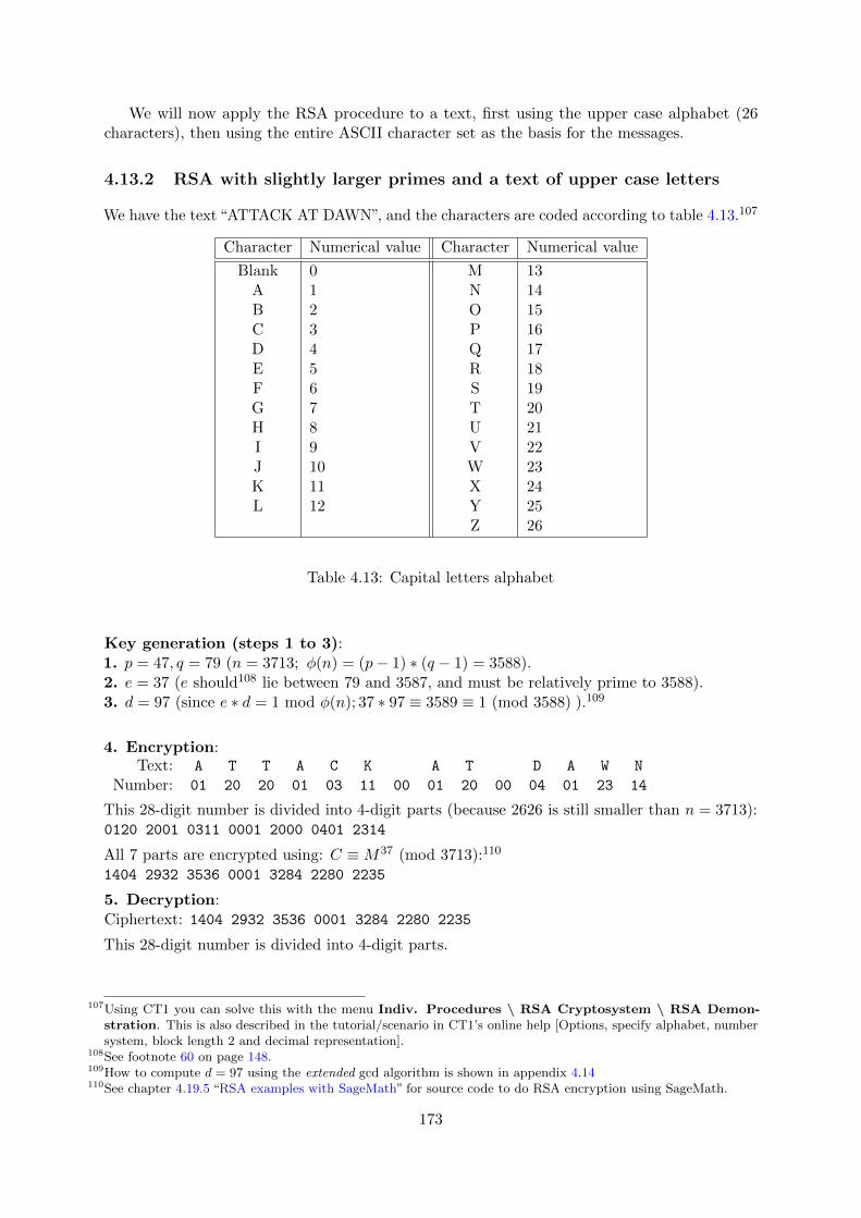
We will now apply the RSA procedure to a text, first using the upper case alphabet (26characters), then using the entire ASCII character set as the basis for the messages.
4.13.2 RSA with slightly larger primes and a text of upper case letters
We have the text “ATTACK AT DAWN”, and the characters are coded according to table 4.13.107
Character Numerical value Character Numerical value
Blank 0 M 13A 1 N 14B 2 O 15C 3 P 16D 4 Q 17E 5 R 18F 6 S 19G 7 T 20H 8 U 21I 9 V 22J 10 W 23K 11 X 24L 12 Y 25
Z 26
Table 4.13: Capital letters alphabet
Key generation (steps 1 to 3):1. p = 47, q = 79 (n = 3713; φ(n) = (p− 1) ∗ (q − 1) = 3588).2. e = 37 (e should108 lie between 79 and 3587, and must be relatively prime to 3588).3. d = 97 (since e ∗ d = 1 mod φ(n); 37 ∗ 97 ≡ 3589 ≡ 1 (mod 3588) ).109
4. Encryption:Text: A T T A C K A T D A W N
Number: 01 20 20 01 03 11 00 01 20 00 04 01 23 14
This 28-digit number is divided into 4-digit parts (because 2626 is still smaller than n = 3713):0120 2001 0311 0001 2000 0401 2314
All 7 parts are encrypted using: C ≡M37 (mod 3713):110
1404 2932 3536 0001 3284 2280 2235
5. Decryption:Ciphertext: 1404 2932 3536 0001 3284 2280 2235
This 28-digit number is divided into 4-digit parts.
107Using CT1 you can solve this with the menu Indiv. Procedures \ RSA Cryptosystem \ RSA Demon-stration. This is also described in the tutorial/scenario in CT1’s online help [Options, specify alphabet, numbersystem, block length 2 and decimal representation].
108See footnote 60 on page 148.109How to compute d = 97 using the extended gcd algorithm is shown in appendix 4.14110See chapter 4.19.5 “RSA examples with SageMath” for source code to do RSA encryption using SageMath.
173
All 7 parts are decrypted using: M ≡ C97 (mod 3713):0120 2001 0311 0001 2000 0401 2314
The 2-digit numbers are transformed into capital letters and blanks.
Using the selected values it is easy for a cryptanalyst to derive the secret values from the publicparameters n = 3713 and e = 37 by revealing that 3713 = 47 ∗ 79.
If n is a 1024-bit number, there is, according to present knowledge, little chance of this.
4.13.3 RSA with even larger primes and a text made up of ASCII characters
In real life, the ASCII alphabet is used to code the individual characters of the message as 8-bitnumbers.
The idea for this exercise111 is taken from the example in [Eck14, p. 271].
Coded in decimal notation, the text “RSA works!” is as follows:Text: R S A w o r k s !
Number: 82 83 65 32 119 111 114 107 115 33
We will work through the example in 2 variants. The steps 1 to 3 are common for both.
Key generation (steps 1 to 3):1. p = 503, q = 509 (n = 256, 027; φ(n) = (p− 1)(q − 1) = 255, 016 = 23 ∗ 127 ∗ 251).112
2. e = 65, 537(e should113 lie between 509 and 255, 015, and must114 be relatively prime to 255, 016).
3. d = 231, 953(since e ≡ d−1 mod φ(n) : 65, 537 ∗ 231, 953 ≡ 15, 201, 503, 761 ≡ 1 (mod 255, 016)).115
Variant 1: All ASCII characters are en-/decrypted separately (no blocks areformed).
4. Encryption:Text: R S A w o r k s !
Number: 82 83 65 32 119 111 114 107 115 33
The letters are not combined!116
Each character is encrypted using: C = M65,537 (mod 256, 027):117
111Using CT1 you can solve this exercise via the menu path Indiv. Procedures \ RSA Cryptosystem \ RSADemonstration.Using JCT you can solve this exercise via the menu path Visuals \ RSA Cryptosystem of the DefaultPerspective.
112See chapter 4.19.5 “RSA examples with SageMath” for the source code to factorize the number φ(n) usingSageMath.
113See footnote 60 on page 148.114e cannot, therefore, be 2, 127 or 251 (65, 537 = 216 + 1) (255, 016 = 23 ∗ 127 ∗ 251).
In real life, φ(n) is not factorized but rather the Euclidean algorithm is used for the selected e to guarantee thatgcd(e, φ(n)) = 1.
115Other possible combinations of (e, d) include: (3, 170, 011), (5, 204, 013), (7, 36, 431).116For secure procedures we need large numbers that assume – as far as possible – all values up to n−1. If the possible
value set for the numbers in the message is too small, even large prime numbers cannot make the procedure secure.An ASCII character is represented by 8 bits. If we want larger values we must combine several numbers. Twocharacters need 16 bits, whereby the maximum value that can be represented is 65536. The modulus n must thenbe greater than 216 = 65536. This is applied in variant 2. When the numbers are combined, the leading zeros arekept in binary notation (just as if we were to write all numbers with 3 digits in decimal notation above and werethen to obtain the sequence 082 083, 065 032, 119 111, 114 107, 115 033).
117See chapter 4.19.5 “RSA examples with SageMath” for the source code for RSA exponentiation using SageMath.
174

212984 025546 104529 031692 248407
100412 054196 100184 058179 227433
5. Decryption:Ciphertext:
212984 025546 104529 031692 248407
100412 054196 100184 058179 227433
Each character is decrypted using: M ≡ C231,953 mod 256, 027:82 83 65 32 119 111 114 107 115 33
Variant 2: The ASCII characters are en-/decrypted two at a time as blocks.
In variant 2 the block formation is done in two different sub-variants: (4./5. and 4’./5’.).
Text: R S A w o r k s !
Number: 82 83 65 32 119 111 114 107 115 33
4. Encryption:Blocks are formed118 (each ASCII character is encoded into a 8 digit binary number and twobinary numbers are joined):21075 16672 30575 29291 29473119
Each block is encrypted using: C ≡M65,537 (mod 256, 027):120
158721 137346 37358 240130 112898
5. Decryption:Ciphertext:158721 137346 37358 240130 112898
Each block is decrypted using: M ≡ C231,953 (mod 256, 027):21075 16672 30575 29291 29473
4’. Encryption:Blocks are formed: (each ASCII character is encoded into a 3 digit decimal number below):82083 65032 119111 114107 115033121
Each block is encrypted using: C ≡M65,537 (mod 256, 027):122
198967 051405 254571 115318 014251
5’. Decryption:
118Forming a block:single character binary representation decimal representation
01010010, 82 01010010 01010011 = 21075
01010011, 83
01000001, 65 01000001 00100000 = 16672
00100000, 32
01110111, 119 01110111 01101111 = 30575
01101111, 111
01110010, 114 01110010 01101011 = 29291
01101011, 107
01110011, 115 01110011 00100001 = 29473
00100001, 33:119In CT1 you can solve this with the menu Indiv. Procedures \ RSA Cryptosystem \ RSA Demonstration
with the following options: all 256 ASCII characters, b-adic, block length 2 and decimal representation.120See chapter 4.19.5 “RSA examples with SageMath” for the source code for RSA exponentiation using SageMath.121The RSA encryption works correctly with the modulus n = 256.027 because each ASCII block of two characters
will be encoded into a number that is smaller or equal than the number 255, 255.122See chapter 4.19.5 “RSA examples with SageMath” for the source code for RSA exponentiation using SageMath.
175

Ciphertext:198967 051405 254571 115318 014251
Each block is decrypted using: M ≡ C2473 (mod 67, 519):82083 65032 119111 114107 115033
176

4.13.4 A small RSA cipher challenge (1)
The task is taken from [Sti06, Exercise 4.6]: The pure solution has been published by Prof.Stinson.123 However, it is not the result that is important here but rather the individual steps ofthe solution, that is, the explanation of the cryptanalysis.124
Two samples of RSA ciphertext are presented in Tables 4.14125 and 4.15126. Your task is todecrypt them. The public parameters of the system are
n = 18, 923 and e = 1261 (for Table 4.14) andn = 31, 313 and e = 4913 (for Table 4.15).
This can be accomplished as follows. First, factor n (which is easy because it is so small).Then compute the exponent d from φ(n), and, finally, decrypt the ciphertext. Use the square-and-multiply algorithm to exponentiate modulo n.
In order to translate the plaintext back into ordinary English text, you need to know howalphabetic characters are “encoded” as elements in Zn. Each element of Zn represents threealphabetic characters as in the following examples:
DOG 7→ 3 ∗ 262 + 14 ∗ 26 + 6 = 2398CAT 7→ 2 ∗ 262 + 0 ∗ 26 + 19 = 1371ZZZ 7→ 25 ∗ 262 + 25 ∗ 26 + 25 = 17, 575.
You will have to invert this process as the final step in your program.
The first plaintext was taken from “The Diary of Samuel Marchbanks”, by Robertson Davies,1947, and the second was taken from “Lake Wobegon Days”, by Garrison Keillor, 1985.
123http://cacr.uwaterloo.ca/~dstinson/solns.html124The method of solving the problem is outlined in the scenario of the online help to CT1 and in the presentation
on the CT website.125The numbers of this table can be worked with via Copy and Paste.126The numbers of this table are in the online help of CT1 in the chapter“Example illustrating the RSA demonstration”.
177

12423 11524 7243 7459 14303 6127 10964 16399
9792 13629 14407 18817 18830 13556 3159 16647
5300 13951 81 8986 8007 13167 10022 17213
2264 961 17459 4101 2999 14569 17183 15827
12693 9553 18194 3830 2664 13998 12501 18873
12161 13071 16900 7233 8270 17086 9792 14266
13236 5300 13951 8850 12129 6091 18110 3332
15061 12347 7817 7946 11675 13924 13892 18031
2620 6276 8500 201 8850 11178 16477 10161
3533 13842 7537 12259 18110 44 2364 15570
3460 9886 8687 4481 11231 7547 11383 17910
12867 13203 5102 4742 5053 15407 2976 9330
12192 56 2471 15334 841 13995 17592 13297
2430 9741 11675 424 6686 738 13874 8168
7913 6246 14301 1144 9056 15967 7328 13203
796 195 9872 16979 15404 14130 9105 2001
9792 14251 1498 11296 1105 4502 16979 1105
56 4118 11302 5988 3363 15827 6928 4191
4277 10617 874 13211 11821 3090 18110 44
2364 15570 3460 9886 9988 3798 1158 9872
16979 15404 6127 9872 3652 14838 7437 2540
1367 2512 14407 5053 1521 297 10935 17137
2186 9433 13293 7555 13618 13000 6490 5310
18676 4782 11374 446 4165 11634 3846 14611
2364 6789 11634 4493 4063 4576 17955 7965
11748 14616 11453 17666 925 56 4118 18031
9522 14838 7437 3880 11476 8305 5102 2999
18628 14326 9175 9061 650 18110 8720 15404
2951 722 15334 841 15610 2443 11056 2186
Table 4.14: RSA ciphertext A
178

6340 8309 14010 8936 27358 25023 16481 25809
23614 7135 24996 30590 27570 26486 30388 9395
27584 14999 4517 12146 29421 26439 1606 17881
25774 7647 23901 7372 25774 18436 12056 13547
7908 8635 2149 1908 22076 7372 8686 1304
4082 11803 5314 107 7359 22470 7372 22827
15698 30317 4685 14696 30388 8671 29956 15705
1417 26905 25809 28347 26277 7897 20240 21519
12437 1108 27106 18743 24144 10685 25234 30155
23005 8267 9917 7994 9694 2149 10042 27705
15930 29748 8635 23645 11738 24591 20240 27212
27486 9741 2149 29329 2149 5501 14015 30155
18154 22319 27705 20321 23254 13624 3249 5443
2149 16975 16087 14600 27705 19386 7325 26277
19554 23614 7553 4734 8091 23973 14015 107
3183 17347 25234 4595 21498 6360 19837 8463
6000 31280 29413 2066 369 23204 8425 7792
25973 4477 30989
Table 4.15: RSA ciphertext B
179

4.13.5 A small RSA cipher challenge (2)
The following task is a corrected version from the book written by Prof. Yan [Yan00, Example3.3.7, p. 318]. However, it is not the result that is important here but rather the individual stepsof the solution, that is, the explanation of the cryptanalysis.127
There are three tasks with completely different degrees of difficulty here. In each case weknow the ciphertext and the public key (e, n):
(a) Known plaintext: find the secret key d using the additionally known original message.
(b) Ciphertext-only: find d and the plaintext.
(c) Calculate the RSA modulus, in other words factorization (with no knowledge of themessage).
n = 63978486879527143858831415041, e = 17579
Message128:
1401202118011200,
1421130205181900,
0118050013010405,
0002250007150400
Cipher:
45411667895024938209259253423,
16597091621432020076311552201,
46468979279750354732637631044,
32870167545903741339819671379
Comment:The original message consisted of a sentence containing 31 characters (coded with the capitalletters alphabet from section 4.13.2). Each group of 16 decimal numbers is then combined toform one number (the last number is filled with zeros). These numbers are raised to the powerof e.
When you decrypt the message you must fill the calculated numbers with leading zeros inorder to obtain plaintext.
This needs to be stressed because the type of padding is extremely important duringimplementation and standardization for interoperable algorithms.
127The method of solving the problem is outlined in the scenario of the online help to CT1 and in the CrypToolpresentation.
128The numbers of this table are in the online help of CT1 in the chapter“Example illustrating the RSA demonstration”.
180
4.14 Appendix: The greatest common divisor (gcd) of wholenumbers and the two algorithms of Euclid129
The greatest common divisor of two natural numbers a and b is an important value that can becalculated very quickly. Here we make use of the fact that if a number c divides the numbers aand b (i.e. there exists an a′ and a b′ such that a = a′ ∗ c and b = b′ ∗ c), then c also divides theremainder r of a/b. In short notion we can write: If c divides a and b it follows that c dividesr = a− ba/bc ∗ b.130
As the latter statement is valid for each common divisor c of a and b it follows that:
gcd(a, b) = gcd(a− ba/bc ∗ b, b).
Using this information, the algorithm for calculating the gcd of two numbers can be written asfollows (in pseudo code):
INPUT: a,b != 0
1. if ( a < b ) then x = a; a = b; b = x; // Swap a and b (a > b)
2. a = a - int(a/b) * b // a is smaller than b, the
// gcd(a, b) is unchanged
3. if ( a != 0 ) then goto 1. // a falls after each step and
// the algorithm ends when a==0.
OUTPUT "gcd(a,b) = " b // b is the gcd of the original a and b
Also further relationships can be derived from the gcd: For this, we need the set of equationsfor a and b:
a = 1 ∗ a+ 0 ∗ bb = 0 ∗ a+ 1 ∗ b,
or, in matrix notation: (ab
)=
(1 00 1
)∗(ab
).
We summarize this information in the extended matrix:(a | 1 0b | 0 1
)If we apply the above gcd algorithm to this matrix, we obtain the extended Euclid algorithm131
which can be used to calculate the multiplicative inverse:
129With the educational tool for number theory NT you can seea) how Euklid’s algorithm calculates the gcd (learning unit 1.3, pages 14-19/21) andb) how Euklid’s enhanced algorithm finds the multiplicative inverse (learning unit 2.2, page 13/40).NT can be called in CT1 via the menu path Indiv. Procedures \ Number Theory Interactive \ LearningTool for Number Theory. See appendix A.6.
CT2 contains within the crypto tutorial “World of Primes ⇒ Number Theory ⇒ Number-theoretic functions”the functions “Extended Euclidian algorithm” and “Modular multiplicative inverse”.
In JCT you can find it in the default perspective via the menu item Visuals \ Extended Euclidian /Reciprocal Subtraction.
130The Gauss bracket bxc of a real number x is defined via: bxc is the next integer less or equal x.See footnote 134 on page 184.
131A more intuitive and generic way from the simple to the extended Euclidean algorithm can be found within theseries RSA & Co. at school: Modern cryptology, old mathematics, and subtle protocols: see NF part 2 [WS06].
181
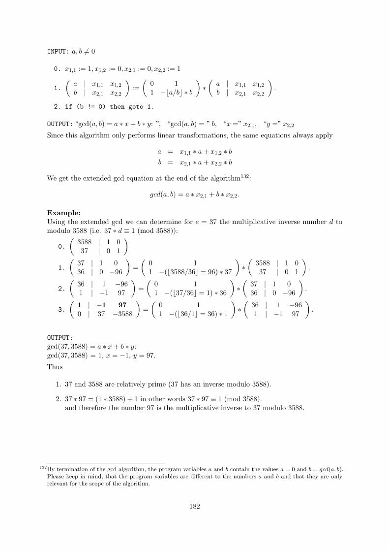
INPUT: a, b 6= 0
0. x1,1 := 1, x1,2 := 0, x2,1 := 0, x2,2 := 1
1.
(a | x1,1 x1,2b | x2,1 x2,2
):=
(0 11 −ba/bc ∗ b
)∗(a | x1,1 x1,2b | x2,1 x2,2
).
2. if (b != 0) then goto 1.
OUTPUT: “gcd(a, b) = a ∗ x+ b ∗ y: ”, “gcd(a, b) = ” b, “x =” x2,1, “y =” x2,2
Since this algorithm only performs linear transformations, the same equations always apply
a = x1,1 ∗ a+ x1,2 ∗ bb = x2,1 ∗ a+ x2,2 ∗ b
We get the extended gcd equation at the end of the algorithm132:
gcd(a, b) = a ∗ x2,1 + b ∗ x2,2.
Example:Using the extended gcd we can determine for e = 37 the multiplicative inverse number d tomodulo 3588 (i.e. 37 ∗ d ≡ 1 (mod 3588)):
0.
(3588 | 1 037 | 0 1
)1.
(37 | 1 036 | 0 −96
)=
(0 11 −(b3588/36c = 96) ∗ 37
)∗(
3588 | 1 037 | 0 1
).
2.
(36 | 1 −961 | −1 97
)=
(0 11 −(b37/36c = 1) ∗ 36
)∗(
37 | 1 036 | 0 −96
).
3.
(1 | −1 970 | 37 −3588
)=
(0 11 −(b36/1c = 36) ∗ 1
)∗(
36 | 1 −961 | −1 97
).
OUTPUT:
gcd(37, 3588) = a ∗ x+ b ∗ y:gcd(37, 3588) = 1, x = −1, y = 97.
Thus
1. 37 and 3588 are relatively prime (37 has an inverse modulo 3588).
2. 37 ∗ 97 = (1 ∗ 3588) + 1 in other words 37 ∗ 97 ≡ 1 (mod 3588).and therefore the number 97 is the multiplicative inverse to 37 modulo 3588.
132By termination of the gcd algorithm, the program variables a and b contain the values a = 0 and b = gcd(a, b).Please keep in mind, that the program variables are different to the numbers a and b and that they are onlyrelevant for the scope of the algorithm.
182

4.15 Appendix: Forming closed sets
The property of closeness within a set is always defined in relation to an operation. The followingshows how to construct the “closed set”G with respect to the operation + (mod 8) for a giveninitial set G0:
G0 = {2, 3} − −−addition of the numbers in G0 determines further numbers :
2 + 3 ≡ 5 (mod 8) = 5
2 + 2 ≡ 4 (mod 8) = 4
3 + 3 ≡ 6 (mod 8) = 6
G1 = {2, 3, 4, 5, 6} − −−addition of the numbers in G1 determines :
3 + 4 ≡ 7 (mod 8) = 7
3 + 5 ≡ 8 (mod 8) = 0
3 + 6 ≡ 9 (mod 8) = 1
G2 = {0, 1, 2, 3, 4, 5, 6, 7} − −−addition of the numbers in G2 does not extend the set!
G3 = G2 −−−we say : G2 is closed for addition (mod 8).
4.16 Appendix: Comments on modulo subtraction
Comment on subtraction modulo 5: 2− 4 = −2 ≡ 3 mod 5.It is therefore not true that −2 ≡ 2 mod 5 !
People often make the mistake of equating this. You can see this clearly if you place thepermutation (0, 1, 2, 3, 4) in Z5, for example from −11 to +11, over the range of numbers in Z.
4 1 2 3 4 1 2 3 4 1 2 3 4 1 2
-11 -1-2-3-4-6-7-8-9 1 2 3 4 6 7
3 4 1
8 9 11
0 0 0 00
0-5 5 10-10
range of numbers modulo 5
range of numbers in Z
183
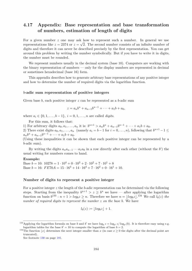
4.17 Appendix: Base representation and base transformationof numbers, estimation of length of digits
For a given number z one may ask how to represent such a number. In general we userepresentations like z = 2374 or z =
√2. The second number consists of an infinite number of
digits and therefore it can never be described precisely by the first representation. You can getaround this problem by writing the number symbolically. But if you have to write it in digits,the number must be rounded.
We represent numbers usually in the decimal system (base 10). Computers are working withthe binary representation of numbers — only for the display numbers are represented in decimalor sometimes hexadecimal (base 16) form.
This appendix describes how to generate arbitrary base representations of any positive integerand how to determine the number of required digits via the logarithm function.
b-adic sum representation of positive integers
Given base b, each positive integer z can be represented as a b-adic sum
z = anbn + an−1b
n−1 + · · ·+ a1b+ a0,
where ai ∈ {0, 1, . . . , b− 1}, i = 0, 1, . . . , n are called digits.
For this sum, it follows that:1) For arbitrary digits a0, a1, . . . , an it is: bn+1 > anb
n + an−1bn−1 + · · ·+ a1b+ a0.
2) There exist digits a0, a1, . . . , an (namely ai = b− 1 for i = 0, . . . , n), following that bn+1− 1 ≤anb
n + an−1bn−1 + · · ·+ a1b+ a0.
(Using these inequalities it can be shown that each positive integer can be represented by ab-adic sum).
By writing the digits anan−1 · · · a1a0 in a row directly after each other (without the bi) theusual writing for numbers comes to hand.
Example:Base b = 10: 10278 = 1 · 104 + 0 · 103 + 2 · 102 + 7 · 101 + 8Base b = 16: FE70A = 15 · 164 + 14 · 163 + 7 · 162 + 0 · 161 + 10.
Number of digits to represent a positive integer
For a positive integer z the length of the b-adic representation can be determined via the followingsteps. Starting from the inequality bn+1 > z ≥ bn we have — after applying the logarithmfunction on basis b133 : n+ 1 > logbz ≥ n. Therefore we have n = blogbzc.134 We call lb(z) thenumber of required digits to represent the number z on the base b. We have
lb(z) := blogbzc+ 1.
133Applying the logarithm formula on base b and b′ we have logb z = logb′ z/ logb′(b). It is therefore easy using e.g.logarithm tables for the base b′ = 10 to compute the logarithm of base b = 2.
134The function bxc determines the next integer smaller than x (in case x ≥ 0 the digits after the decimal point aretruncated).See footnote 130 on page 181.
184

Example 1 (decimal→hex):We compute for the decimal number z = 234 (EA in hex) the hexadecimal representation(number base b = 16)
l16(z) = blog16(z)c+ 1 = bln(z)/ ln(16)c+ 1 = b1.96...c+ 1 = 1 + 1 = 2.
Example 2 (decimal→binary):We compute for the decimal number z = 234 (11101010 in binary) the binary representation(number base b = 2)
l2(z) = blog2(z)c+ 1 = bln(z)/ ln(2)c+ 1 = b7.87...c+ 1 = 7 + 1 = 8.
Example 3 (binary→decimal):We compute for the decimal number z = 11101010 (234 decimal) the decimal representation(number base b = 10)
l10(z) = blog10(z)c+ 1 = bln(z)/ ln(10)c+ 1 = b2, 36...c+ 1 = 2 + 1 = 3.
Algorithm to compute the base representation
Given the number z one can compute the base b representation of z using the following algorithm:
input: z, bn := 0, z′ := zwhile z′ > 0 do
an := z′ mod b,z′ := bz′/bcn := n+ 1
end dooutput: anan−1 · · · a1a0 in base b representation.
Example 1 (decimal→hex):The integer z = 234 on the number base 10 will be transformed into the hex representation viaa0 = 234 mod 16 = 10 = A, 234/16 = 14 = E,a1 = 14 mod 16 = Eand therefore we have EA.
Example 2 (binary→decimal):The binary number z = 1000100101110101 is transformed into the decimal representation viathe following steps:1000100101110101 = 1001 (mod 1010) =⇒ a0 = 9, 1000100101110101/1010 = 110110111110110110111110 = 1000 (mod 1010) =⇒ a1 = 8, 110110111110/1010 = 101011111101011111 = 1 (mod 1010) =⇒ a2 = 1, 10101111/1010 = 100011100011 = 101 (mod 1010) =⇒ a3 = 5, 100011/1010 = 111 = 11 (mod 1010) =⇒ a4 = 3therefore z = 35189.
185

4.18 Appendix: Interactive presentation about the RSA cipher
The folowing presentation (last update Nov. 2010) shows the basics of the RSA cipher in aninteractive way.
There are three variants:
• Powerpoint 2007 (for download; dynamical, animated)135
• PDF (for download; static, no interaction)136
• Flash (can be started within the browser, requires JavaScript; time-controlled replay)137
Figure 4.4: Screenshot RSA Presentation (PDF)
135http://www.cryptool.org/images/ct1/presentations/RSA/RSA-en.pptx136http://www.cryptool.org/images/ct1/presentations/RSA/RSA-en(keine%20Interaktivitaet).pdf137http://www.cryptool.org/images/ct1/presentations/RSA/RSA-Flash-en/player.html
186

4.19 Appendix: Examples using SageMath
“She would never be able to tell her parents ... about any of this. She couldn’t tell them abouther code-breaking work. About her near death at the hands of the Daemon. About the shadowy
entities pulling the strings of her government.”
Quote 14: Daniel Suarez138
Below you can find SageMath source code related to contents of the chapter 4 (“Introduction toElementary Number Theory with Examples”).
4.19.1 Multiplication table modulo m
The multiplication table 4.4 (from page 130) for a× i (mod m), where m = 17, a = 5 and a = 6,and i ranges over all integers from 0 to 16 can be computed using SageMath as follows:
SageMath sample 4.3 Multiplication tables for a× i (mod m) with m = 17, a = 5 and a = 6sage: m = 17; a = 5; b = 6
sage: [mod(a * i, m).lift() for i in xrange(m)]
[0, 5, 10, 15, 3, 8, 13, 1, 6, 11, 16, 4, 9, 14, 2, 7, 12]
sage: [mod(b * i, m).lift() for i in xrange(m)]
[0, 6, 12, 1, 7, 13, 2, 8, 14, 3, 9, 15, 4, 10, 16, 5, 11]
The function mod() returns an object that represents integers modulo m (in our case m = 17).From the Mod object you can get its single components either with the function component
or with the function lift. We use the method lift() to convert that object to an integerrepresentation.
The other multiplication table examples modulo 13 (table 4.5) and modulo 12 (table 4.6) onpage 130 can similarly be computed by replacing m = 17 with m = 13 and m = 12 respectively.
4.19.2 Fast exponentiation
The fast exponentiation modulo m can be computed using the SageMath function power_mod().The result of this function is an integer. We can compute the exponentiation in the example inchapter “Fast calculation of high powers” on page 133 as follows:
SageMath sample 4.4 Fast exponentiation mod m = 103sage: a = 87; m = 103
sage: exp = [2, 4, 8, 16, 32, 43]
sage: [power_mod(a, e, m) for e in exp]
[50, 28, 63, 55, 38, 85]
138Daniel Suarez, “Freedom”, Dutton Adult, 2010, Chapter 19, “Crossroad”, p. 229, Philips.
187

4.19.3 Multiplicative order
The order ordm(a) of a number a in the multiplicative group Z∗m is the smallest number i ≥ 1such that ai ≡ 1 (mod m) holds (see chapter 4.9, “Multiplicative order and primitive roots”).To create table 4.7 on page 141 we can print all exponentiation ai (mod 11) as follows:
SageMath sample 4.5 Table with all powers ai (mod m) for m = 11, a = 1, ..., 10sage: m = 11
sage: for a in xrange(1, m):
....: print [power_mod(a, i, m) for i in xrange(1, m)]
....:
[1, 1, 1, 1, 1, 1, 1, 1, 1, 1]
[2, 4, 8, 5, 10, 9, 7, 3, 6, 1]
[3, 9, 5, 4, 1, 3, 9, 5, 4, 1]
[4, 5, 9, 3, 1, 4, 5, 9, 3, 1]
[5, 3, 4, 9, 1, 5, 3, 4, 9, 1]
[6, 3, 7, 9, 10, 5, 8, 4, 2, 1]
[7, 5, 2, 3, 10, 4, 6, 9, 8, 1]
[8, 9, 6, 4, 10, 3, 2, 5, 7, 1]
[9, 4, 3, 5, 1, 9, 4, 3, 5, 1]
[10, 1, 10, 1, 10, 1, 10, 1, 10, 1]
and including the last column with the order of each a mod (11)
sage: m = 11
sage: for a in xrange(1, m):
....: lst= [power_mod(a, i, m) for i in xrange(1, m)]
....: lst.append(multiplicative_order(mod(a,m)))
....: print lst
....:
[1, 1, 1, 1, 1, 1, 1, 1, 1, 1, 1]
[2, 4, 8, 5, 10, 9, 7, 3, 6, 1, 10]
[3, 9, 5, 4, 1, 3, 9, 5, 4, 1, 5]
[4, 5, 9, 3, 1, 4, 5, 9, 3, 1, 5]
[5, 3, 4, 9, 1, 5, 3, 4, 9, 1, 5]
[6, 3, 7, 9, 10, 5, 8, 4, 2, 1, 10]
[7, 5, 2, 3, 10, 4, 6, 9, 8, 1, 10]
[8, 9, 6, 4, 10, 3, 2, 5, 7, 1, 10]
[9, 4, 3, 5, 1, 9, 4, 3, 5, 1, 5]
[10, 1, 10, 1, 10, 1, 10, 1, 10, 1, 2]
188

Table 4.8 on page 142 gives examples for the order modulo 45 ord45(a) and the Euler numberφ(45).
The following SageMath code constructs a table similar to that on page 142.
SageMath sample 4.6 Table with all powers ai (mod 45) for a = 1, ..., 12 plus the order of asage: m = 45
sage: for a in xrange(1, 13):
....: lst = [power_mod(a, i, m) for i in xrange(1, 13)]
....: try:
....: lst.append(multiplicative_order(mod(a, m)))
....: except:
....: lst.append("None")
....: lst.append(euler_phi(m))
....: print lst
....:
[1, 1, 1, 1, 1, 1, 1, 1, 1, 1, 1, 1, 1, 24]
[2, 4, 8, 16, 32, 19, 38, 31, 17, 34, 23, 1, 12, 24]
[3, 9, 27, 36, 18, 9, 27, 36, 18, 9, 27, 36, ’None’, 24]
[4, 16, 19, 31, 34, 1, 4, 16, 19, 31, 34, 1, 6, 24]
[5, 25, 35, 40, 20, 10, 5, 25, 35, 40, 20, 10, ’None’, 24]
[6, 36, 36, 36, 36, 36, 36, 36, 36, 36, 36, 36, ’None’, 24]
[7, 4, 28, 16, 22, 19, 43, 31, 37, 34, 13, 1, 12, 24]
[8, 19, 17, 1, 8, 19, 17, 1, 8, 19, 17, 1, 4, 24]
[9, 36, 9, 36, 9, 36, 9, 36, 9, 36, 9, 36, ’None’, 24]
[10, 10, 10, 10, 10, 10, 10, 10, 10, 10, 10, 10, ’None’, 24]
[11, 31, 26, 16, 41, 1, 11, 31, 26, 16, 41, 1, 6, 24]
[12, 9, 18, 36, 27, 9, 18, 36, 27, 9, 18, 36, ’None’, 24]
The number ordm(a) only exists if a is relatively prime to m, which can be checked withgcd(a, m).
In the above code example, we put the calculation of the multiplicative order within atry-except block. This allows SageMath to catch any exceptions or errors raised by the functionmultiplicative_order(). If an exception or error is raised in the try block, then we knowthat ordm(a) does not exist for that particular value of a, hence in the except block we appendthe string "None" to the row as represented by the object lst.
189

Table 4.9 on page 143 displays exponentiation ai (mod 46) as well as the order ord46(a).
SageMath can create that table as follows:
SageMath sample 4.7 Table with all powers ai (mod 46) for a = 1, ..., 23 plus the order of asage: m = 46
sage: euler_phi(m)
22
sage: for a in xrange(1, 24):
....: lst = [power_mod(a, i, m) for i in xrange(1, 24)]
....: try:
....: lst.append(multiplicative_order(mod(a, m)))
....: except:
....: lst.append("None")
....: print lst
....:
[1, 1, 1, 1, 1, 1, 1, 1, 1, 1, 1, 1, 1, 1, 1, 1, 1, 1, 1, 1, 1, 1, 1, 1]
[2, 4, 8, 16, 32, 18, 36, 26, 6, 12, 24, 2, 4, 8, 16, 32, 18, 36, 26, 6, 12, 24, 2, ’None’]
[3, 9, 27, 35, 13, 39, 25, 29, 41, 31, 1, 3, 9, 27, 35, 13, 39, 25, 29, 41, 31, 1, 3, 11]
[4, 16, 18, 26, 12, 2, 8, 32, 36, 6, 24, 4, 16, 18, 26, 12, 2, 8, 32, 36, 6, 24, 4, ’None’]
[5, 25, 33, 27, 43, 31, 17, 39, 11, 9, 45, 41, 21, 13, 19, 3, 15, 29, 7, 35, 37, 1, 5, 22]
[6, 36, 32, 8, 2, 12, 26, 18, 16, 4, 24, 6, 36, 32, 8, 2, 12, 26, 18, 16, 4, 24, 6, ’None’]
[7, 3, 21, 9, 17, 27, 5, 35, 15, 13, 45, 39, 43, 25, 37, 29, 19, 41, 11, 31, 33, 1, 7, 22]
[8, 18, 6, 2, 16, 36, 12, 4, 32, 26, 24, 8, 18, 6, 2, 16, 36, 12, 4, 32, 26, 24, 8, ’None’]
[9, 35, 39, 29, 31, 3, 27, 13, 25, 41, 1, 9, 35, 39, 29, 31, 3, 27, 13, 25, 41, 1, 9, 11]
[10, 8, 34, 18, 42, 6, 14, 2, 20, 16, 22, 36, 38, 12, 28, 4, 40, 32, 44, 26, 30, 24, 10, ’None’]
[11, 29, 43, 13, 5, 9, 7, 31, 19, 25, 45, 35, 17, 3, 33, 41, 37, 39, 15, 27, 21, 1, 11, 22]
[12, 6, 26, 36, 18, 32, 16, 8, 4, 2, 24, 12, 6, 26, 36, 18, 32, 16, 8, 4, 2, 24, 12, ’None’]
[13, 31, 35, 41, 27, 29, 9, 25, 3, 39, 1, 13, 31, 35, 41, 27, 29, 9, 25, 3, 39, 1, 13, 11]
[14, 12, 30, 6, 38, 26, 42, 36, 44, 18, 22, 32, 34, 16, 40, 8, 20, 4, 10, 2, 28, 24, 14, ’None’]
[15, 41, 17, 25, 7, 13, 11, 27, 37, 3, 45, 31, 5, 29, 21, 39, 33, 35, 19, 9, 43, 1, 15, 22]
[16, 26, 2, 32, 6, 4, 18, 12, 8, 36, 24, 16, 26, 2, 32, 6, 4, 18, 12, 8, 36, 24, 16, ’None’]
[17, 13, 37, 31, 21, 35, 43, 41, 7, 27, 45, 29, 33, 9, 15, 25, 11, 3, 5, 39, 19, 1, 17, 22]
[18, 2, 36, 4, 26, 8, 6, 16, 12, 32, 24, 18, 2, 36, 4, 26, 8, 6, 16, 12, 32, 24, 18, ’None’]
[19, 39, 5, 3, 11, 25, 15, 9, 33, 29, 45, 27, 7, 41, 43, 35, 21, 31, 37, 13, 17, 1, 19, 22]
[20, 32, 42, 12, 10, 16, 44, 6, 28, 8, 22, 26, 14, 4, 34, 36, 30, 2, 40, 18, 38, 24, 20, ’None’]
[21, 27, 15, 39, 37, 41, 33, 3, 17, 35, 45, 25, 19, 31, 7, 9, 5, 13, 43, 29, 11, 1, 21, 22]
[22, 24, 22, 24, 22, 24, 22, 24, 22, 24, 22, 24, 22, 24, 22, 24, 22, 24, 22, 24, 22, 24, 22, ’None’]
[23, 23, 23, 23, 23, 23, 23, 23, 23, 23, 23, 23, 23, 23, 23, 23, 23, 23, 23, 23, 23, 23, 23, ’None’]
190

The following code for generating the tables 4.10 and 4.11 at page 145 f. also delivers theresult in a way, that in can be easily processed in LaTeX. The prerequisite is that all content isassigned to one SageMath object (here a matrix).139
SageMath sample 4.8 Code for tables with all powers ai (mod m) for variable a and i plusorder of a and Eulerphi of mdef power_mod_order_matrix(m, max_a, max_i):
r = matrix(ZZ, max_a+1, max_i+3)
for a in xrange(0, max_a+1):
r[a, 0] = a
for i in xrange(1, max_i+1):
if a==0:
r[a,i] = i
else:
r[a, i] = power_mod(a, i, m)
try:
r[a, max_i+1] = multiplicative_order(mod(a, m))
except:
r[a, max_i+1] = 0
r[a, max_i+2] = euler_phi(m)
return r
print "\n1: m=45;max_i=13;max_a=13";m=45;max_i=13;max_a=13
r = power_mod_order_matrix(m, max_a, max_i);print r;print latex(r)
print "\n2: m=46;max_i=25;max_a=25";m=46;max_i=25;max_a=25
r = power_mod_order_matrix(m, max_a, max_i);print r.str();print latex(r)
print "\n3: m=14;max_i=13;max_a=16";m=14;max_i=13;max_a=16
r = power_mod_order_matrix(m, max_a, max_i);print r;print latex(r)
print "\n4: m=22;max_i=21;max_a=25";m=22;max_i=21;max_a=25
r = power_mod_order_matrix(m, max_a, max_i);print r.str();print latex(r)
...
3: m=14;max_i=13;max_a=16
[ 0 1 2 3 4 5 6 7 8 9 10 11 12 13 0 6]
[ 1 1 1 1 1 1 1 1 1 1 1 1 1 1 1 6]
[ 2 2 4 8 2 4 8 2 4 8 2 4 8 2 0 6]
[ 3 3 9 13 11 5 1 3 9 13 11 5 1 3 6 6]
...
\left(\begin{array}{rrrrrrrrrrrrrrrr}
0 & 1 & 2 & 3 & 4 & 5 & 6 & 7 & 8 & 9 & 10 & 11 & 12 & 13 & 0 & 6\\
1 & 1 & 1 & 1 & 1 & 1 & 1 & 1 & 1 & 1 & 1 & 1 & 1 & 1 & 1 & 6\\
2 & 2 & 4 & 8 & 2 & 4 & 8 & 2 & 4 & 8 & 2 & 4 & 8 & 2 & 0 & 6\\
3 & 3 & 9 & 13 & 11 & 5 & 1 & 3 & 9 & 13 & 11 & 5 & 1 & 3 & 6 & 6\\
...
139Remark about the SageMath program, especially the SageMath indices:• for x in xrange(2, 5) delivers 2,3,4.• m = matrix(ZZ, 2, 5) has 2 rows and 5 columns.
The cells are named m(0,0) to m(1,4).• All elements of the matrix have to be numerical, so “0” instead of “None” as in the tables before.• The output of matrices can be controlled in SageMath with:
sage: from sage.matrix.matrix0 import set_max_cols, set_max_rows
sage: set_max_cols(100)
sage: set_max_rows(100)
• The length of the cycle in the last column of the tables 4.10 and 4.11 was added manually.
191
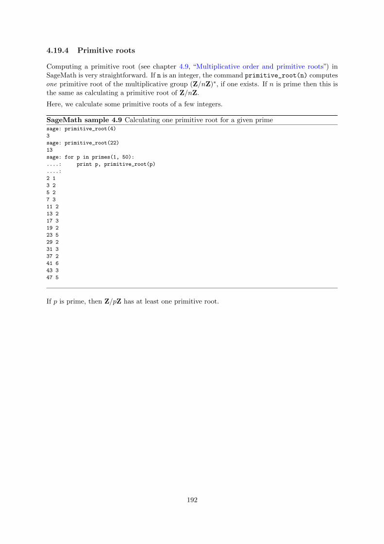
4.19.4 Primitive roots
Computing a primitive root (see chapter 4.9, “Multiplicative order and primitive roots”) inSageMath is very straightforward. If n is an integer, the command primitive_root(n) computesone primitive root of the multiplicative group (Z/nZ)∗, if one exists. If n is prime then this isthe same as calculating a primitive root of Z/nZ.
Here, we calculate some primitive roots of a few integers.
SageMath sample 4.9 Calculating one primitive root for a given primesage: primitive_root(4)
3
sage: primitive_root(22)
13
sage: for p in primes(1, 50):
....: print p, primitive_root(p)
....:
2 1
3 2
5 2
7 3
11 2
13 2
17 3
19 2
23 5
29 2
31 3
37 2
41 6
43 3
47 5
If p is prime, then Z/pZ has at least one primitive root.
192

Sometimes we want to compute all the primitive roots of (Z/nZ)∗, not just any primitive rootof (Z/nZ)∗. The following self-written function can do this.140
SageMath sample 4.10 Function “enum PrimitiveRoots of an Integer” to calculate all primi-tive roots for a given numberdef enum_PrimitiveRoots_of_an_Integer(M):
r"""
Return all the primitive roots of the integer M (if possible).
"""
try:
g = primitive_root(M)
except:
return None
targetOrder = euler_phi(M)
L=[]
# Stepping through all odd integers from 1 up to M, not including
# M. So this loop only considers values of i where 1 <= i < M.
for i in xrange(1,M,2):
testGen = Mod(g^i,M)
if testGen.multiplicative_order() == targetOrder:
L.append(testGen.lift())
# removing duplicates
return Set(L)
# AA_Start -- Testcases for enum_PrimitiveRoots_of_an_Integer(M)
print "AA_Start -- Testcases for enum_PrimitiveRoots_of_an_Integer(M)"
M=10; print "1-----------Testcase: M = %s" % M
LL = enum_PrimitiveRoots_of_an_Integer(M)
if LL==None:
print M
else:
print LL
M=8; print "2-----------Testcase: M = %s" % M
# M=8 hat keine primitive root mod m. Checke, ob per try - except abgefangen.
LL = enum_PrimitiveRoots_of_an_Integer(M)
if LL==None:
print M
else:
print LL
M=17; print "3-----------Testcase: M = %s" % M
LL = enum_PrimitiveRoots_of_an_Integer(M)
if LL==None:
print M
else:
print LL
# AA_End -- Testcases
OUTPUT:
AA_Start -- Testcases for enum_PrimitiveRoots_of_an_Integer(M)
1-----------Testcase: M = 10
{3, 7}
2-----------Testcase: M = 8
8
3-----------Testcase: M = 17
{3, 5, 6, 7, 10, 11, 12, 14}
140This code was developed in a SageMath script file and executed non-interactively. That is why you don’t see“sage:” and “....:” at the beginning of the lines like in the SageMath samples before.
193
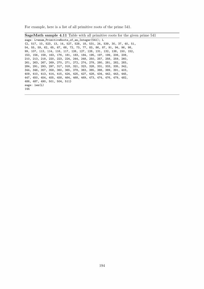
For example, here is a list of all primitive roots of the prime 541.
SageMath sample 4.11 Table with all primitive roots for the given prime 541sage: L=enum_PrimitiveRoots_of_an_Integer(541); L
{2, 517, 10, 523, 13, 14, 527, 528, 18, 531, 24, 539, 30, 37, 40, 51,
54, 55, 59, 62, 65, 67, 68, 72, 73, 77, 83, 86, 87, 91, 94, 96, 98,
99, 107, 113, 114, 116, 117, 126, 127, 128, 131, 132, 138, 150, 152,
153, 156, 158, 163, 176, 181, 183, 184, 195, 197, 199, 206, 208,
210, 213, 218, 220, 223, 224, 244, 248, 250, 257, 258, 259, 260,
261, 263, 267, 269, 270, 271, 272, 274, 278, 280, 281, 282, 283,
284, 291, 293, 297, 317, 318, 321, 323, 328, 331, 333, 335, 342,
344, 346, 357, 358, 360, 365, 378, 383, 385, 388, 389, 391, 403,
409, 410, 413, 414, 415, 424, 425, 427, 428, 434, 442, 443, 445,
447, 450, 454, 455, 458, 464, 468, 469, 473, 474, 476, 479, 482,
486, 487, 490, 501, 504, 511}
sage: len(L)
144
194

With a little bit of programming, we can count how many primitive roots are in a given range ofintegers. We can check this for all numbers or only for the primes within this range.
SageMath sample 4.12 Function “count PrimitiveRoots of an IntegerRange” to calculate allprimitive roots for a given range of integersdef count_PrimitiveRoots_of_an_IntegerRange(start, end, bPrimesOnly=True):
r"""
Compute all primitive roots of all numbers between start and end,
inclusive, and count them.
If the flag bPrimesOnly is True, it performs primality tests, so it
allows us to count the number of primes from start to end, inclusive.
If the flag bPrimesOnly is false, it additionally counts these even
numbers which have no primitive root.
"""
nCheckedNumb = 0
nCheckedNumb_WithoutPrimitivRoots = 0
nPrimitiveRoots = 0
for n in xrange(start, end+1):
if bPrimesOnly:
if is_prime(n):
nCheckedNumb += 1
L = enum_PrimitiveRoots_of_an_Integer(n)
nPrimitiveRoots += len(L)
else:
nCheckedNumb += 1
L = enum_PrimitiveRoots_of_an_Integer(n)
if L==None:
nCheckedNumb_WithoutPrimitivRoots += 1
else:
nPrimitiveRoots += len(L)
if bPrimesOnly:
print "Found all %s" % nPrimitiveRoots + \
" primitive roots of %s primes." % nCheckedNumb
else:
if nCheckedNumb_WithoutPrimitivRoots == 0:
print "Found all %s " % nPrimitiveRoots + \
"primitive roots of %s numbers." % nCheckedNumb
else:
print "Found all %s " % nPrimitiveRoots + \
"primitive roots of %s numbers." % \
(nCheckedNumb - nCheckedNumb_WithoutPrimitivRoots)
print "(Total of numbers checked: %s, " % nCheckedNumb + \
"Amount of numbers without primitive roots: %s)" % \
nCheckedNumb_WithoutPrimitivRoots
195

Using the SageMath command time, we can also find out how long it takes on our computer.
SageMath sample 4.13 Function “count PrimitiveRoots of an IntegerRange”: testcases andoutput# BB_Start -- Testcases for count_PrimitiveRoots_of_an_IntegerRange(start, end, bPrimesOnly=True)
print "\n\nBB_Start -- Testcases for count_PrimitiveRoots_of_an_IntegerRange(start, end, True)"
print "\n1-----------Testcase: (1, 500)"
time count_PrimitiveRoots_of_an_IntegerRange(1, 500)
print "\n2-----------Testcase: (5, 6, False)"
time count_PrimitiveRoots_of_an_IntegerRange(5, 6, False)
print "\n3-----------Testcase: (1, 500, False)"
time count_PrimitiveRoots_of_an_IntegerRange(1, 500, False)
# BB_End -- Testcases
OUTPUT:
BB_Start -- Testcases for count_PrimitiveRoots_of_an_IntegerRange(start, end, bPrimesOnly=True)
1-----------Testcase: (1, 500)
Found all 8070 primitive roots of 95 primes.
Time: CPU 0.94 s, Wall: 0.97 s
2-----------Testcase: (5, 6, False)
Found all 3 primitive roots of 2 numbers.
Time: CPU 0.00 s, Wall: 0.00 s
3-----------Testcase: (1, 500, False)
Found all 11010 primitive roots of 170 numbers.
(Total of numbers checked: 500, Amount of numbers without primitive roots: 330)
Time: CPU 1.52 s, Wall: 1.59 s
196

Using our custom-defined function enum_PrimitiveRoots_of_an_Integer, we can find allprimitive roots of one prime integer p.
The following function counts how many primes are in a given range and enumerates alltheir primitive roots.
From this list of primitive roots, we can determine the smallest and largest primitive root forZ/pZ, as well as count the number of primitive roots of Z/pZ.
SageMath sample 4.14 Function “count PrimitiveRoots of a PrimesRange” to calculate thenumber of primitive roots for a given range of primesdef count_PrimitiveRoots_of_a_PrimesRange(start, end):
r"""
Compute all primitive roots of all primes between start and end,
inclusive. This uses a primes iterator.
"""
nPrimes = 0
nPrimitiveRoots = 0
for p in primes(start, end+1):
L = enum_PrimitiveRoots_of_an_Integer(p)
print p, len(L)
nPrimes += 1
nPrimitiveRoots += len(L)
print "Found all %s" % nPrimitiveRoots + " primitive roots of %s primes." % nPrimes
# CC_Start -- Testcases for count_PrimitiveRoots_of_a_PrimesRange(start, end)
print "\n\nBB_Start -- Testcases for count_PrimitiveRoots_of_a_PrimesRange(start, end)"
print "-----------Testcase: (1, 1500)"
time count_PrimitiveRoots_of_a_PrimesRange(1, 1500)
# CC_End -- Testcases
OUTPUT:
CC_Start -- Testcases for count_PrimitiveRoots_of_a_PrimesRange(start, end)
-----------Testcase: (1, 1500)
2 1
3 1
5 2
7 2
11 4
13 4
17 8
19 6
23 10
29 12
31 8
37 12
...
1483 432
1487 742
1489 480
1493 744
1499 636
Found all 62044 primitive roots of 239 primes.
Time: CPU 7.55 s, Wall: 7.85 s
197
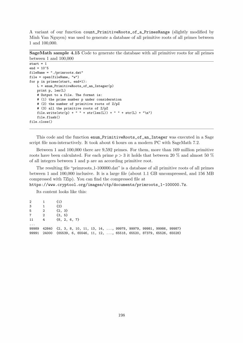
A variant of our function count_PrimitiveRoots_of_a_PrimesRange (slightly modified byMinh Van Nguyen) was used to generate a database of all primitive roots of all primes between1 and 100,000.
SageMath sample 4.15 Code to generate the database with all primitive roots for all primesbetween 1 and 100,000start = 1
end = 10^5
fileName = "./primroots.dat"
file = open(fileName, "w")
for p in primes(start, end+1):
L = enum_PrimitiveRoots_of_an_Integer(p)
print p, len(L)
# Output to a file. The format is:
# (1) the prime number p under consideration
# (2) the number of primitive roots of Z/pZ
# (3) all the primitive roots of Z/pZ
file.write(str(p) + " " + str(len(L)) + " " + str(L) + "\n")
file.flush()
file.close()
This code and the function enum_PrimitiveRoots_of_an_Integer was executed in a Sagescript file non-interactively. It took about 6 hours on a modern PC with SageMath 7.2.
Between 1 and 100,000 there are 9,592 primes. For them, more than 169 million primitiveroots have been calculated. For each prime p > 3 it holds that between 20 % and almost 50 %of all integers between 1 and p are an according primitive root.
The resulting file “primroots 1-100000.dat” is a database of all primitive roots of all primesbetween 1 and 100,000 inclusive. It is a large file (about 1.1 GB uncompressed, and 156 MBcompressed with 7Zip). You can find the compressed file athttps://www.cryptool.org/images/ctp/documents/primroots_1-100000.7z.
Its content looks like this:
2 1 {1}
3 1 {2}
5 2 {2, 3}
7 2 {3, 5}
11 4 {8, 2, 6, 7}
...
99989 42840 {2, 3, 8, 10, 11, 13, 14, ..., 99978, 99979, 99981, 99986, 99987}
99991 24000 {65539, 6, 65546, 11, 12, ..., 65518, 65520, 87379, 65526, 65528}
198

The Sage script 4.16 calculates all primitive roots for all primes up to one million, andoutputs for each prime the number of different primitive roots and the smallest primitive root.
SageMath sample 4.16 Code to generate the database with the smallest primitive root forall primes between 1 and 1,000,000start = 1
end = 10^6
fileName = "./primroot-smallest_up-to-one-million.dat"
file = open(fileName, "w")
file.write(timestring + "\n")
file.flush()
for p in primes(start, end+1):
L = enum_PrimitiveRoots_of_an_Integer(p)
# Output to commandline only p and number of prim roots of Z_p
print p, len(L)
# Output more to a file. The format is:
# (1) the prime number p under consideration
# (2) the number of primitive roots of Z_p
# (3) the smallest primitive roots of Z_p
LL = sorted(L) # necessary as the smallest primroot is not always
# found first by the enum fct (see L of p=43)
file.write(str(p) + " " + str(len(L)) + " " + str(LL[0]) + "\n")
file.flush()
file.flush()
file.close()
The Sage script 4.16 was stopped after several weeks (running on a modern PC withSageMath 7.2) after investigating all primes up to half a million. The result was stored in thefile “primroot number-of-and-smallest up-to-prime-500107.dat”, which is 617 kB uncompressed,and 178 kB compressed with 7Zip.
You can find the compressed file at https://www.cryptool.org/images/ctp/documents/primroot_number-of-and-smallest_up-to-prime-500107.7z.
This database contains all primes p between 1 and 500,107 together with the accordingnumber of primitive roots and the according smallest prim root mod p. It holds that the numberof primitive roots (for p > 3 )is always an odd number. We don’t know a formula which deliversthe number of primitive roots for a given number. So this database may be interesting to somenumber theorists.141 Its content looks like this:
2 1 1
3 1 2
5 2 2
7 2 3
11 4 2
13 4 2
17 8 3
...
99989 42840 2
99991 24000 6
100003 28560 2
...
500069 250032 2
500083 151520 2
500107 156864 2
141See Re: [sage-devel] What can we do with a database of primitive roots?https://groups.google.com/forum/m/#!topic/sage-devel/TA5Nk2GdhOI
199

If you are looking only for the smallest primitive root, then this script could be accelerateddramatically by applying mathematical theory and searching more directly for possible candidates(instead of first generating all primitive roots with enum_PrimitiveRoots_of_an_Integer).
200

The database file “primroots 1-100000.dat” then was used as input to create three graphics usingthe following code (Sage script 4.17).
SageMath sample 4.17 Code to generate the graphics about the primitive rootssage: # open a database file on primitive roots from 1 to 100,000
sage: file = open("/scratch/mvngu/primroots.dat", "r")
sage: plist = [] # list of all primes from 1 to 100,000
sage: nlist = [] # number of primitive roots modulo prime p
sage: minlist = [] # smallest primitive root modulo prime p
sage: maxlist = [] # largest primitive root modulo prime p
sage: for line in file:
....: # get a line from the database file and tokenize it for processing
....: line = line.strip().split(" ", 2)
....: # extract the prime number p in question
....: plist.append(Integer(line[0]))
....: # extract the number of primitive roots modulo p
....: nlist.append(Integer(line[1]))
....: # extract the list of all primitive roots modulo p
....: line = line[-1]
....: line = line.replace("{", "")
....: line = line.replace("}", "")
....: line = line.split(", ")
....: # sort the list in non-decreasing order
....: line = [Integer(s) for s in line]
....: line.sort()
....: # get the smallest primitive root modulo p
....: minlist.append(line[0])
....: # get the largest primitive root modulo p
....: maxlist.append(line[-1])
....:
sage: file.close() # close the database file
sage: # plot of number of primitive roots modulo p
sage: nplot = point2d(zip(plist, nlist), pointsize=1)
sage: nplot.axes_labels(["x", "y"])
sage: nplot
sage: # plot of smallest primitive root modulo prime p
sage: minplot = point2d(zip(plist, minlist), pointsize=1)
sage: minplot.axes_labels(["x", "y"])
sage: minplot
sage: # plot of largest primitive root modulo prime p
sage: maxplot = point2d(zip(plist, maxlist), pointsize=1)
sage: maxplot.axes_labels(["x", "y"])
sage: maxplot
201

Figure 4.5 graphs the number of primitive roots for each prime between 1 and 100,000. Thex-axis represents primes between 1 and 100,000, while the y-axis counts the number of primitiveroots for each prime within that interval.
Figure 4.5: The number of primitive roots of all primes between 1 and 100,000.
Figure 4.6 graphs the smallest primitive roots of all primes between 1 and 100,000. Thex-axis represents primes between 1 and 100,000. The y-axis represents the smallest primitiveroot of each prime within that interval.
Figure 4.7 shows a corresponding graph for the largest primitive root of each prime withinthe above interval.
202

Figure 4.6: The smallest primitive roots of all primes between 1 and 100,000.
Figure 4.7: The largest primitive roots of all primes between 1 and 100,000.
203

4.19.5 RSA examples with SageMath
Below is SageMath source code for the simple RSA examples in section 4.13 (“The RSA procedurewith actual numbers”).
Example on page 173:The RSA exponentiation M37 (mod 3713) on message M = 120 can be calculated in SageMathas follows:
sage: power_mod(120, 37, 3713)
1404
Example on page 174:The factorization of φ(256027) = 255016 = 23 ∗ 127 ∗ 251 can be calculated using SageMath asfollows:
SageMath sample 4.18 Factoring a numbersage: factor(255016)
2^3 * 127 * 251
Example on page 174:SageMath can do RSA encryption as follows:
SageMath sample 4.19 RSA encryption by modular exponentiation of a number (used asmessage)sage: A = [82, 83, 65, 32, 119, 111, 114, 107, 115, 33]
sage: e = 65537; m = 256027
sage: [power_mod(a, e, m) for a in A]
[212984, 25546, 104529, 31692, 248407, 100412, 54196, 100184, 58179, 227433]
Example on page 175:RSA encryption using SageMath:
sage: A = [21075, 16672, 30575, 29291, 29473]
sage: e = 65537; m = 256027
sage: [power_mod(a, e, m) for a in A]
[158721, 137346, 37358, 240130, 112898]
Example on page 175:RSA encryption using SageMath:
sage: A = [82083, 65032, 119111, 114107, 115033]
sage: e = 65537; m = 256027
sage: [power_mod(a, e, m) for a in A]
[198967, 51405, 254571, 115318, 14251]
204

4.19.6 How many private RSA keys d exist within a given modulo range?
The RSA encryption procedure was described in section 4.10.2 (“How the RSA procedure works”).Steps 1 to 3 constitute key generation, steps 4 and 5 are the encryption:
1. Select two distinct random prime numbers p and q and calculate n = p ∗ q.The value n is called the RSA modulus.
2. Select an arbitrary e ∈ {2, · · · , n− 1} such that:e is relatively prime to φ(n) = (p− 1) ∗ (q − 1).We can then “throw away” p and q.
3. Select d ∈ {1, · · · , n− 1} with e ∗ d ≡ 1 (mod φ(n)),i.e. d is the multiplicative inverse of e modulo φ(n). We can then “throw away” φ(n).
→ (n, e) is the public key P .→ (n, d) is the private key S (only d must be kept secret).
4. For encryption, the message represented as a (binary) number is divided into parts suchthat each part of the number represents a number less than n.
5. Encryption of the plaintext (or the parts of it) M ∈ {1, · · · , n− 1}:
C = E((n, e);M) := M e (mod n).
The default way to crack a given RSA ciphertext C would be to use the public key of therecipient and to try to factorize n. Then you can go through the steps 2 and 3 and generate theprivate key e, which is normally used to decrypt a ciphertext.
According to the “prime number theorem”142 the number of prime numbers PI(x) is asymp-totic to x/ln(x). Between 1 and a given n there are about n/ln(n) different primes.
If you don’t want to use factorization but ask the question like in classic encryption, you maywant to find out: How many possible private keys (n, d) are there for a given key size rangen ∈ [a, b]?143
SageMath source code 4.20 below defining the function count_Number_of_RSA_Keys can answerthis question concretely (if the modulus is not too big).144
As there are many more private keys (n, d) within a bigger range of values for n, even brute-forcefactoring is much more efficient as brute-force trying all the keys.
142See section 3.7.2 (“Density and distribution of the primes”).143Chapter 4.8.5 (“How many private RSA keys d are there modulo 26”), p. 139 deals with the special case n = 26.144
a) Calling sage: count_Number_of_RSA_Keys(100, 1000) means to consider the interval [100, 1000] for n.n is defined by the two primes p, q : n = p ∗ q.So here one prime can have the maximal value 500 because 2 ∗ 500 = 1000 (while then the other primewill have the smallest possible prime value 2).
The number of possible combinations of primes is comb = 258.The number of primes in the given range is 143.The number of private keys is 34, 816.
b) Calling sage: count_Number_of_RSA_Keys(100, 100, True) has the following output:- Number of private keys for modulus in a given range: 0- Number of primes in a given range: 0The reason for that is, that with this call only n = 100 is considered, and the function investigates onlysemiprime n: 100 is not semi prime , this means 100 is not the product of only two primes.
205

SageMath sample 4.20 How many private RSA keys d are there if you know a range for thepublic key n?def count_Number_of_RSA_Keys(start, end, Verbose=False):
r"""
How many private RSA keys (n,d) exist, if only modulus N is given, and start <= N <= end?
(prime_range(u,o) delivers all primes >=u und < o).
"""
a = start
b = end
s = 0
comb = 0
for p in prime_range(1, b/2+1):
for q in prime_range(p + 1, b/2+1):
if a <= p * q and p * q <= b:
comb = comb +1
s = s + (euler_phi(euler_phi(p * q))-1)
if Verbose:
print "p=%s, " % p + "q=%s, " % q + "s=%s" % s
print "Number of private keys d for modulus in a given range: %s" % s + " (comb=%s), " % comb
# Just for comparison: How many primes are in this range?
s = 0
for p in prime_range(a, b+1):
if Verbose:
print "a=%s, " % a + "b=%s, " % b + "p=%s" % p
s = s + 1
print "Number of primes in a given range: %s" % s
print "\n\nDD_Start -- Testcases for count_Number_of_RSA_Keys(start, end)"
print "\n-----------Testcase: (100, 1000) [Should deliver 34.816]"
time count_Number_of_RSA_Keys(100, 1000)
print "\n-----------Testcase: (100, 107, True) [Should deliver 23]"
time count_Number_of_RSA_Keys(100, 107, True)
u = 10^3; o = 10^4;
print "\n-----------Testcase: (%s, " % u + "%s) [Should deliver 3.260.044]" % o
time count_Number_of_RSA_Keys(u, o)
OUTPUT:
DD_Start -- Testcases for count_Number_of_RSA_Keys(start, end)
-----------Testcase: (100, 1000) [Should deliver 34.816]
Number of private keys d for modulus in a given range: 34816 (comb=258),
Number of primes in a given range: 143
Time: CPU 0.03 s, Wall: 0.04 s
-----------Testcase: (100, 107, True) [Should deliver 23]
p=2, q=53, s=23
Number of private keys d for modulus in a given range: 23 (comb=1),
a=100, b=107, p=101
a=100, b=107, p=103
a=100, b=107, p=107
Number of primes in a given range: 3
Time: CPU 0.00 s, Wall: 0.00 s
-----------Testcase: (1000, 10000) [Should deliver 3,260,044]
Number of private keys d for modulus in a given range: 3260044 (comb=2312),
Number of primes in a given range: 1061
Time: CPU 0.63 s, Wall: 0.66 s
206

4.19.7 RSA fixed points me = m mod n mit m ∈ {1, ..., n− 1}
Also encryption methods can have fixed – cleartext messages where the according ciphertextmatches the original. In mathematics, variables mapped by the algorithm (function) ontothemselves are called fixed points. In cryptography the according messages are called“unconcealedmessages”.
Generally speaking: The more fixed points an encryption algorithm contains, the easier it isto break it.
With the RSA procedure: n = pq is the product of two different prime numbers, and thereexists e where gcd(e, (p− 1)(q − 1)) = 1. The encription is then c = me mod n. A fixed pointin the RSA procedure is a message m, where: m = me mod n. The result of the encryption isthe given message.
When the size of n is sufficiently big, the probability of the occurance of fixed points in RSAis very small – as illustrated in Figure 4.8: In average, we found not more than 40 fixed points.
Students often presume the occurence of fixed points high, because they counter a “relatively”large number of examples when experimenting with small prime numbers, as m = 0, 1 and n-1are also always fixed points.
In practice, where large prime numbers are chosen, fixed points have no significance for thesecurity of RSA. Therefore, this paragraph refers more to the mathematical questions.145
4.19.7.1 The number of RSA fixed points
In this section we show how many RSA fixed points there are for m ∈ {1, ..., n− 1}.
Theorem 4.19.1. The number of the fixed points me = m mod n with m ∈ {1, ..., n− 1} isgcd(p− 1, e− 1) · gcd(q − 1, e− 1).
ProofGiven me = m mod n. According to the CRT146, the following statements are equivalent:
[me = m mod n] ⇔ [me = m mod p and me = m mod q]
Furthermore, the decomposition on the right side is equivalent to:
me−1 = 1 mod p and me−1 = 1 mod q.
We consider me−1 = 1 mod p and search all (e− 1) roots of unity147 in Z∗p.It holds: Z∗p for p prime is cyclic. ⇒ A generator g exists which produces Z∗p: Z∗p =< g >.
145Thanks to Taras Shevchenko for gathering parts of the content of this section and to Volker Simon for writing theSageMath program 4.21 “Getfixpoints”.
146CRT = Chinese Remainder Theorem. http://en.wikipedia.org/wiki/Chinese_Remainder_Theorem147- In mathematics, a root of unity is a number x that equals 1 when raised to some integer power n.
- An n-th root of unity x is primitive if it is not a k-th root of unity for all integers k smaller than n:
xn = 1 and xk 6= 1 (k = 1, 2, 3, ..., n− 1)
- If F is a finite field and n is a positive integer, then a nth-root of unity in F is a solution of the equation
xn − 1 = 0 in F
207

The following theorem from [Kat01, Pg. 69] characterizes all (e− 1)-th roots of unity in Z∗p:
Theorem 4.19.2. gα is exactly then (e−1)-th root of unity in Z∗p, when (e−1)α = 0 mod p−1.There are gcd(p− 1, e− 1) of these.
ProofThe first theorem results directly from the small theorem from Fermat:
gα(e−1) = 1 mod p ⇒ α(e− 1) = 0 mod p− 1
Let δ = gcd(p− 1, e− 1). α(e− 1) = 0 mod p− 1 implies α(e−1)δ = 0 mod p−1
δ .
Since e−1δ and p−1
δ are coprime (each was reduced by the gcd of their corresponding numerator),
α must be a multiple of p−1δ .
αp− 1
δwith α = 1, ..., δ
These δ different powers then correspond to the (e− 1)-th roots of unity gαp−1δ mod p in Z∗p. 2
Analog for q: For me−1 = 1 mod q we then have gcd(q − 1, e− 1) many of (e− 1)-th roots ofunity.
The number of combinations of the (e− 1)-th root of unity in Z∗p and Z∗q gives the total quantityof RSA fixed points: me = m mod n with m ∈ {1, ..., n− 1}:gcd(p− 1, e− 1) · gcd(q − 1, e− 1)
Adding m = 0 to the above, results in the theorem 4.19.3:
Theorem 4.19.3. If m ∈ {0, ..., n− 1}, then the quantity of the RSA fixed points is:
(gcd(p− 1, e− 1) + 1) · (gcd(q − 1, e− 1) + 1)
2
4.19.7.2 Lower bound for the quantity of RSA fixed points
In the following section, we show that there is a lower bound for the quantity of RSA fixedpoints. This lower bound 6 exists when the two different RSA prime numbers are the smallestpossible values (2 and 3).
Theorem 1: Given: p = 2, q = 3The quantity of RSA fixed points for p = 2 and q = 3 is(gcd(p− 1, e− 1)︸ ︷︷ ︸
=1
+1) · (gcd(q − 1, e− 1)︸ ︷︷ ︸=2
+1) = 2 · 3 = 6
Theorem 2: Given: p 6= q; p > 2, q > 2The quantity of RSA fixed points for p 6= q; p, q > 2 is ≥ 9.
Proof (of the 2nd theorem)Since p and q are prime, (p− 1) and (q − 1) for p, q > 2 are even.The RSA algorithm requires to choose e so that 1 < e < φ(n) = (p− 1)(q − 1) and
208

gcd(e, (p− 1)(q − 1)) = 1Since (p− 1) and (q − 1) are even, e is odd ⇒ e− 1 is even.Since (p− 1) and (e− 1) are even, then:gcd(p− 1, e− 1) ≥ 2⇒ (gcd(p− 1, e− 1) + 1) ≥ 3 and (gcd(q − 1, e− 1) + 1) ≥ 3⇒ (gcd(p− 1, e− 1) + 1) · (gcd(q − 1, e− 1) + 1) ≥ 9 2
Samples:For (e, n) = (17, 6), all six possible messages {0,1,2,3,4,5} are fixed points (for n = 6, it isindependent from the value of e).For (e, n) = (17, 10), all 10 possible messages are fixed points.For (e, n) = (19, 10), only 6 of the 10 possible messages are fixed points.
4.19.7.3 Unfortunate choice of e
In this section, we show that with e = 1 + lcm(p− 1, q − 1) each encryption results in a fixedpoint (independently of the size of p, q, or n, each m is mapped on itself); and then we generalizethis to all unfortunate choices of e.
If e = 1, then for all m: c = me = m. This is the trivial case.
Theorem: Given: p, q > 2If e = 1 + lcm(p− 1, q − 1), then for all m ∈ {1, ..., n− 1}: me = m mod n.
ProofGiven:- e · d = 1 mod φ(n) or e · d = 1 mod lcm(p− 1, q − 1)- mx mod n = mx mod φ(n) mod n
Encryption of messages:c = me mod n, where c is the ciphertext and m is the plaintext.
Decryption of messages:m′ = cd mod n, where d is the multiplicative inverse of e.
We will show: c = m mod n for the chosen e.
c = me mod n
c = m1+lcm(p−1,q−1) mod n
c = m1 ·mk·(p−1)·(q−1) mod n
c = m1 ·m[k·φ(n)] mod φ(n) mod n
c = m1 ·m0 = m mod n 2
209

Example: Fixed point property for all m:Given n = p · q = 13 · 37 = 481⇒ φ(n) = (p− 1)(q − 1) = 12 · 36 = 432⇒ e = lcm(p− 1, q − 1) + 1 = lcm(12, 36) + 1 = 36 + 1 = 37.With m ∈ {4, 6, 7, 480} we get in me mod n as:437 mod 481 = 4637 mod 481 = 6737 mod 481 = 748037 mod 481 = 480
There is not just the one single e (see above), where all m ∈ {1, ..., n− 1} have the fixed pointproperty me = m mod n.148
Theorem 4.19.4. The complete fixed point property of all m is valid for every e = j · lcm(p−1, q − 1) + 1, where j = 0, 1, 2, 3, 4, ... to e ≤ φ(n).
Example: Further values for e with fixed point properties:Given n = p · q = 13 · 37 = 481 with lcm(p− 1, q − 1) = lcm(12, 36) = 36.Then, e can have the following values: e = j · lcm(p− 1, q − 1) + 1 for j = 0, 1, 2, ..., 11:⇒ e ∈ {1, 37, 73, 109, 145, 181, 217, 253, 289, 325, 361, 397}.
Starting j = 12, the following is valid: e = 12 · lcm(12, 36) + 1 = 432 + 1 = 433 > 432 = φ(n).
Checking the four values above for m with e = 217, the results are:4217 mod 481 = 46217 mod 481 = 67217 mod 481 = 7480217 mod 481 = 480
Theorem 4.19.5. The number of possible values for e with me = m mod n may be computedwith the following:
[Quantity e] =
⌊φ(n)
lcm(p− 1, q − 1) + 1
⌋+ 1 =
φ(n)
lcm(p− 1, q − 1)
In our example, this results in 432lcm(12,36) = 12 different values for e, where me = m mod n for all
m in Z481.
148Sometimes these e, which make any message to a fixed point, are called “weak keys” (e, n) of the RSA algorithm.This notation is different to the “weak keys” k in DES, where every message m relates to itself if the encryptionis done twice. To my knowledge, for larger n the RSA procedure does not have weaks in this meaning: (me)e = m.In JCT you can find weak DES keys in the default perspective via the menu item Visuals \ Inner States ofthe Data Encryption Standard (DES).
210

4.19.7.4 An empirical estimate of the quantity of fixed points for growing moduli
In this section, we make an empirical estimate of the quantity of fixed points for growing moduli(and e not weak).
For this, we randomly choose p and q from the six following ranges each characterized by itslower and upper bound: (22, 210), (210, 220), (220, 240), (240, 280), (280, 2160), (2160, 2320).10 attempts were made for each range. For the exponent e, the standard value e = 216 + 1 wasalways chosen. The quantity of fixed points for all 60 attempts was computed with the program4.21 “Getfixpoints.sage”.
The following five sets contain the randomly chosen value pairs (p,q) of the first five ranges.
From(22, 210) : (p, q) ∈ {(127, 947), (349, 809), (47, 461), (587, 151), (19, 23),
(709, 509), (653, 11), (859, 523), (823, 811), (83, 331)}
From(210, 220) : (p, q) ∈ {(447401, 526283), (474223, 973757), (100829, 126757),
(35803, 116933), (577751, 598783), (558121, 607337),
(950233, 248167), (451103, 73009), (235787, 164429),
(433267, 287939)}
From(220, 240) : (p, q) ∈ {(58569604997, 321367332149), (286573447351, 636576727223),
(134703821971, 134220414529), (161234614601, 711682765579),
(19367840881, 804790726361), (932891507377, 521129503333),
(337186437739, 426034644493), (986529569219, 604515928397),
(276825557171, 654134442649), (639276602353, 1069979301731)}
From(240, 280) : (p, q) ∈ {(667530919106151273090539, 287940270633610590682889),
(437090557112369481760661, 590040807609821698387141),
(1131921188937480863054851, 813935599673320990215139)
(874130181777177966406673, 632270193935624953596331),
(599303355925474677078809, 717005631177936134003029),
(752829320004631398659063, 714134510643836818718761),
(1046313315092743492917349, 835721729660755006973833),
(877161707568112212806617, 42831503328261105793649),
(575464819450637793425803, 5425832051159043433027),
(321404337099945148592363, 992663778486687980443879)}
211

From(280, 2160) : (p, q) ∈ {(838952969674957834783403492645269831354775774659,
694309130163549038783972189350416942879771871411),
(981985107290629501374187748859961786804311564643,
178616495258601001174141825667078950281544628693),
(614446632627716919862227545890890553330513965359,
761232454374959264696945191327265643178491649141),
(1421756952722008095585945863962560425554707936337,
986781711714138924140285492105143175328486228197),
(862346475785474165539441761205023498091366178341,
438589995804600940885415547506719456975478582911),
(1034081318899669345416602574034081247538053001533,
1207032778571434704618111297072774884748706223447),
(308083812465705343620096534684980088954958466893,
350597371862294596793629011464584694618569736021),
(830376326124356299120963861338027196931951857769,
924874232653136669722297184352059466357375363191),
(85600581120154590810189237569820706006659829231,
297064381842806596646150718828138629443319259829),
(1358984492013516052055790129324581847590275909129,
609402294805414245544586792657989060761523960427)}
Figure 4.8: An empirical estimate of the quantity of fixed points for growing moduli
Figure 4.8 shows that within the six ranges of size, the average number of fixed points wasnot higher than 40.
212

4.19.7.5 Example: Determining all fixed points for a specific public RSA key
The exercise is to determine all fixed points for (n, e) = (866959, 17).
Solution:We start by factoring n: 866959 = 811 · 1069.
The quantity of RSA fixed points results from the theorem 4.19.3:(gcd(p−1, e−1)+1) ·(gcd(q−1, e−1)+1) = (gcd(811−1, 17−1)+1) ·(gcd(1069−1, 17−1)+1) =(2 + 1) · (4 + 1) = 15
The SageMath program 4.21 (Getfixpoints) returns 15 fixed points for (n, e) = (866959, 17):
0 1 23518 23519 47037
188964 212482 236000 654477 843440
843441 630959 677995 819922 866958
Example:Using 843441 as a sample for validation: 84344117 mod 866959 = 843441So m = 843441 is actually a fixed point for the given (n, e).
Meaning of the Variables in the SageMath Code 4.21:
- gen_f_p = r.multiplicative_generator()
r is a residue class ring modulo p and multiplicative_generator() returns
a generator element that was created by the ring modulo p.
- power_mod(gen_f_p,Integer(i*(p-1)/gcd_p),p)
The power_mod function raises a number m to the power of e and returns the results modulo n.
E.g.: power_mod(m, e, n) := m^e modulo n
- numpy.append(fp,power_mod(gen_f_p,Integer(i*(p-1)/gcd_p),p))
The append function extends an array (fp) by an additional element.
- crt(Integer(r),Integer(s),Integer(p),Integer(q))
CRT is the acronym for Chinese Remainder Theorem. crt(r, s, p, q) solves
the congruences x = r mod p and x = s mod q with the help of the Chinese Remainder Theorem.
213

SageMath sample 4.21 Determining all fixed points for a specific public RSA keyimport numpy
print "--- Search for fixpoints in Textbook-RSA given p, q, e ---";
fp=numpy.array([0])
fq=numpy.array([0])
#Edit e,p,q here
###EDIT BEGIN###
e=17;
p=811;
q=1069;
###EDIT END###
n=p*q;
print "Prime p: ",p;
print "Prime q: ",q;
print "Modul n: ",n;
print "Public exponent e: ", e;
r=Integers(p)
gen_f_p = r.multiplicative_generator(); print "\nGenerator of f_p: ",gen_f_p;
s=Integers(q)
gen_f_q = s.multiplicative_generator(); print "Generator of f_q: ",gen_f_q;
gcd_p = gcd(e-1,p-1)
gcd_q = gcd(e-1,q-1)
print "\ngcd(e-1,p-1): ", gcd_p;
print "gcd(e-1,q-1): ", gcd_q;
print "\nNumber of fixpoints: ",(gcd_p+1)*(gcd_q+1);
#Calculating fixpoints modulo F_p
#run i from 0 until gcd(e-1,p-1):
#g^( i*(p-1) / (gcd(e-1,p-1)) ) mod p
print "\nFixpoints modulo p";
print "0 (trivial fixpoint added manually)";
i=0;
for i in range(gcd_p):
fix_p = power_mod(gen_f_p,Integer(i*(p-1)/gcd_p),p); print fix_p;
fp = numpy.append(fp,fix_p)
print "\nFixpoints modulo q";
print "0 (trivial fixpoint added manually)";
j=0;
for j in range(gcd_q):
fix_q = power_mod(gen_f_q,Integer(j*(q-1)/gcd_q),q); print fix_q;
fq = numpy.append(fq,fix_q);
print "\nFixpoints for the public RSA key (n,e) = (", n, ",", e, ")"
for r in fp:
for s in fq:
print crt(Integer(r),Integer(s),Integer(p),Integer(q))
print "\nRemark: You can verify each fixpoint with power_mod(m,e,n).";
214

4.20 Appendix: List of the definitions and theorems formulatedin this chapter
Short description Page
Definition 4.3.1 prime numbers 120Definition 4.3.2 composite numbers 120
Theorem 4.3.1 factors of composite numbers 121Theorem 4.3.2 1st fundamental theorem of number theory 121
Definition 4.4.1 divisibility 122Definition 4.4.2 remainder class r modulo m 122Definition 4.4.3 congruent 123
Theorem 4.4.1 congruence with difference 123Theorem 4.6.1 multiplicative inverse (existence) 129Theorem 4.6.2 exhaustive permutation 129Theorem 4.6.3 power mod m 132
Definition 4.7.1 Zn 134Definition 4.7.2 Z∗n 135
Theorem 4.7.1 multiplicative inverse in Z∗n 135
Definition 4.8.1 Euler function φ(n) 136Theorem 4.8.1 φ(p) 136Theorem 4.8.2 φ(p ∗ q) 136Theorem 4.8.3 φ(p1 ∗ · · · ∗ pk) 136Theorem 4.8.4 φ(pe11 ∗ · · · ∗ p
ekk ) 136
Theorem 4.8.5 little Fermat 138Theorem 4.8.6 Euler-Fermat theorem 138
Definition 4.9.1 multiplicative order ordm(a) 140Definition 4.9.2 primitive root of m 141Theorem 4.9.1 exhausting of all possible values 143
Theorem 4.19.3 number of RSA fixed points 208
215
Bibliography (Chap NT)
[AKS02] Agrawal, M., N. Kayal, and N. Saxena: PRIMES in P, August 2002. Correctedversion.http://www.cse.iitk.ac.in/~manindra/algebra/primality_v6.pdf,http://fatphil.org/maths/AKS/.
[Bau95] Bauer, Friedrich L.: Entzifferte Geheimnisse. Springer, 1995.
[Bau00] Bauer, Friedrich L.: Decrypted Secrets. Springer, 2nd edition, 2000.
[Ber01] Bernstein, Daniel J.: Circuits for integer factorization: a proposal.http://cr.yp.to/papers/nfscircuit.ps,http://cr.yp.to/djb.html, 2001.
[Ber05] Bernstein, Daniel J.: Factoring into coprimes in essentially linear time. Journal ofAlgorithms, 54, 2005. http://cr.yp.to/lineartime/dcba-20040404.pdf.
[Beu96] Beutelspacher, Albrecht: Kryptologie. Vieweg, 5th edition, 1996.
[BFT02] Bourseau, F., D. Fox, and C. Thiel: Vorzuge und Grenzen des RSA-Verfahrens.Datenschutz und Datensicherheit (DuD), 26:84–89, 2002.http://www.secorvo.de/publikationen/rsa-grenzen-fox-2002.pdf.
[BLP93] Buhler, J. P., H. W. Lenstra, and C. Pomerance: Factoring integers with the numberfield sieve. In Lenstra, K. and H.W. Lenstra (editors): The Development of theNumber Field Sieve, Lecture Notes in Mathematics, Vol. 1554, pages 50–94. Springer,1993.
[BSI16] BSI: Angaben des BSI fur die Algorithmenkataloge der Vorjahre, Empfehlungen zurWahl der Schlussellangen. Technical report, BSI (Bundesamt fur Sicherheit in derInformationstechnik), 2016.https://www.bsi.bund.de/DE/Themen/DigitaleGesellschaft/Elektronisch
eSignatur/TechnischeRealisierung/Kryptoalgorithmen/kryptoalg.html
- Vgl.: BNetzA (Bundesnetzagentur): Jahrlich erscheinende Veroffentlichung zuAlgorithmen und Parametern im Umfeld elektronischer Signaturen:http://www.bundesnetzagentur.de/cln_1411/DE/Service-Funktionen/Elek
tronischeVertrauensdienste/QES/WelcheAufgabenhatdieBundesnetzagentu
r/GeeigneteAlgorithmenfestlegen/geeignetealgorithmenfestlegen_node.
html
- Vgl.: Eine Stellungnahme zu diesen Empfehlungen:http://www.secorvo.de/publikationen/stellungnahme-algorithmenempfehl
ung-020307.pdf .
216

[Eck14] Eckert, Claudia: IT-Sicherheit: Konzepte-Verfahren-Protokolle. De Gruyter Olden-bourg, 9th edition, 2014. Paperback.
[ESS12] Esslinger, B., J. Schneider, and V. Simon: RSA – Sicherheit in der Praxis. KESZeitschrift fur Informationssicherheit, 2012(2):22–27, April 2012.https://www.cryptool.org/images/ctp/documents/kes_2012_RSA_Sicherhe
it.pdf.
[GKP94] Graham, R. E., D. E. Knuth, and O. Patashnik: Concrete Mathemathics, a Founda-tion of Computer Science. Addison Wesley, 6th edition, 1994.
[HDWH12] Heninger, Nadia, Zakir Durumeric, Eric Wustrow, and J. Alex Halderman: MiningYour Ps and Qs: Detection of Widespread Weak Keys in Network Devices. InProceedings of the 21st USENIX Security Symposium, August 2012.https://factorable.net/paper.html.
[Kat01] Katzenbeisser, Stefan: Recent Advances in RSA Cryptography. Springer, 2001.
[Kle10] Kleinjung, Thorsten et al.: Factorization of a 768-bit RSA modulus, version 1.4,2010. http://eprint.iacr.org/2010/006.pdf.
[Knu98] Knuth, Donald E.: The Art of Computer Programming, vol 2: SeminumericalAlgorithms. Addison-Wesley, 3rd edition, 1998.
[LHA+12] Lenstra, Arjen K., James P. Hughes, Maxime Augier, Joppe W. Bos, ThorstenKleinjung, and Christophe Wachter: Ron was wrong, Whit is right, A Sanity Checkof Public Keys Collected on the Web. Cryptology ePrint Archive, February 2012.http://eprint.iacr.org/2012/064.pdf.
[LL93] Lenstra, A. and H. Lenstra: The development of the Number Field Sieve. LectureNotes in Mathematics 1554. Springer, 1993.
[LSTT02] Lenstra, Arjen K., Adi Shamir, Jim Tomlinson, and Eran Tromer: Analysis ofBernstein’s Factorization Circuit, 2002.http://tau.ac.il/~tromer/papers/meshc.pdf.
[LV01] Lenstra, Arjen K. and Eric R. Verheul: Selecting Cryptographic Key Sizes (1999 +2001). Journal of Cryptology, 14:255–293, 2001.http://www.cs.ru.nl/E.Verheul/papers/Joc2001/joc2001.pdf,http://citeseerx.ist.psu.edu/viewdoc/download?doi=10.1.1.20.69&rep=
rep1&type=pdf.
[MvOV01] Menezes, Alfred J., Paul C. van Oorschot, and Scott A. Vanstone: Handbook ofApplied Cryptography. Series on Discrete Mathematics and Its Application. CRCPress, 5th edition, 2001, ISBN 0-8493-8523-7. (Errata last update Jan 22, 2014).http://cacr.uwaterloo.ca/hac/,http://www.cacr.math.uwaterloo.ca/hac/.
[Ngu09] Nguyen, Minh Van: Number Theory and the RSA Public Key Cryptosystem – Anintroductory tutorial on using SageMath to study elementary number theory andpublic key cryptography, 2009. http://faculty.washington.edu/moishe/hanoiex/Number%20Theory%20Applications/numtheory-crypto.pdf.
217

[Oec03] Oechslin, Philippe: Making a Faster Cryptanalytic Time-Memory Trade-Off. Tech-nical report, Crypto 2003, 2003.http://lasecwww.epfl.ch/pub/lasec/doc/Oech03.pdf.
[Pfl97] Pfleeger, Charles P.: Security in Computing. Prentice-Hall, 2nd edition, 1997.
[Pom84] Pomerance, Carl: The Quadratic Sieve Factoring Algorithm. In Blakley, G.R. andD. Chaum (editors): Proceedings of Crypto ’84, LNCS 196, pages 169–182. Springer,1984.
[Sch96] Schneier, Bruce: Applied Cryptography, Protocols, Algorithms, and Source Code inC. Wiley, 2nd edition, 1996.
[Sch04] Schneider, Matthias: Analyse der Sicherheit des RSA-Algorithmus. Mogliche Angrif-fe, deren Einfluss auf sichere Implementierungen und okonomische Konsequenzen.Master’s thesis, Universitat Siegen, 2004.
[Sec02] Security, RSA: Has the RSA algorithm been compromised as a result of Bernstein’sPaper? Technical report, RSA Security, April 2002. http://www.emc.com/emc-
plus/rsa-labs/historical/has-the-rsa-algorithm-been-compromised.htm.
[Sed90] Sedgewick, Robert: Algorithms in C. Addison-Wesley, 1990.
[Sil00] Silverman, Robert D.: A Cost-Based Security Analysis of Symmetric and AsymmetricKey Lengths. RSA Laboratories Bulletin, 13:1–22, April 2000.
[ST03a] Shamir, Adi and Eran Tromer: Factoring Large Numbers with the TWIRL Device,2003. http://www.tau.ac.il/~tromer/papers/twirl.pdf.
[ST03b] Shamir, Adi and Eran Tromer: On the Cost of Factoring RSA-1024. RSA Laborato-ries CryptoBytes, 6(2):11–20, 2003.http://www.tau.ac.il/~tromer/papers/cbtwirl.pdf.
[Sti06] Stinson, Douglas R.: Cryptography – Theory and Practice. Chapman & Hall/CRC,3rd edition, 2006.
[SW10] Schulz, Ralph Hardo and Helmut Witten: Zeitexperimente zur Faktorisierung. EinBeitrag zur Didaktik der Kryptographie. LOG IN, 166/167:113–120, 2010.http://bscw.schule.de/pub/bscw.cgi/d864899/Schulz_Witten_Zeit-
Experimente.pdf.
[Wil95] Wiles, Andrew: Modular elliptic curves and fermat’s last theorem. Annals of Mathe-matics, 141, 1995.
[WLB03] Weis, Rudiger, Stefan Lucks, and Andreas Bogk: Sicherheit von 1024 bit RSA-Schlusseln gefahrdet. Datenschutz und Datensicherheit (DuD), 27(6):360–362, 2003.
[WS06] Witten, Helmut and Ralph Hardo Schulz: RSA & Co. in der Schule: ModerneKryptologie, alte Mathematik, raffinierte Protokolle. NF Teil 2: RSA fur großeZahlen. LOG IN, 2006(143):50–58, 2006.http://bscw.schule.de/pub/bscw.cgi/d404410/RSA_u_Co_NF2.pdf.
[WS08] Witten, Helmut and Ralph Hardo Schulz: RSA & Co. in der Schule: Moderne Kryp-tologie, alte Mathematik, raffinierte Protokolle. NF Teil 3: RSA und die elementareZahlentheorie. LOG IN, 2008(152):60–70, 2008.http://bscw.schule.de/pub/nj_bscw.cgi/d533821/RSA_u_Co_NF3.pdf.
218

[WSE15] Witten, Helmut, Ralph Hardo Schulz, and Bernhard Esslinger: RSA & Co. in derSchule: Moderne Kryptologie, alte Mathematik, raffinierte Protokolle, NF Teil 7:Alternativen zu RSA oder Diskreter Logarithmus statt Faktorisierung. LOG IN,2010(181-182):85–102, 2015.Hierin werden u.a. DH und Elgamal in einem breiteren Kontext behandelt. DieVerfahren werden mit Codebeispielen in Python und SageMath erlautert.http://bscw.schule.de/pub/nj_bscw.cgi/d1024013/RSA_u_Co_NF7.pdf,http://www.log-in-verlag.de/wp-content/uploads/2015/07/Internetquel
len-LOG-IN-Heft-Nr.181-182.doc.
[Yan00] Yan, Song Y.: Number Theory for Computing. Springer, 2000.
All links have been confirmed at July 12, 2016.
219

Web links
1. Ron Knott’s Fibonacci pageHere, everything revolves around Fibonacci numbers.http://www.maths.surrey.ac.uk/hosted-sites/R.Knott/Fibonacci/fib.html
2. CrypToolOpen source e-learning software to illustrate cryptography and cryptanalysishttp://www.cryptool.org
3. MathematicaCommercial mathematics packagehttp://www.wolfram.com
4. LiDIALibrary with number-theory functions and the LC interpreter. Maintenance stopped in2000.http://cs.nyu.edu/exact/core/download/core_v1.3/core_v1.3/lidia/
5. BCInterpreter with number-theory functions. Development stopped since 2006. The existingBC versions don’t work correctly under new Windows versions.Keith Matthews regularily publishes updates for UNIX.http://www.gnu.org/software/bc/bc.html
http://www.numbertheory.org/gnubc/gnubc.html
6. Pari-GPFast and free interpreter with number theoretical functions. Also within the browser.Maintained by Karim Belabas.http://pari.math.u-bordeaux.fr/
http://pari.math.u-bordeaux.fr/gp.html
http://en.wikipedia.org/wiki/PARI/GP
7. SageMathExcellent, open source computer algebra system with Python as script language, used tobuild the code samples in this chapter. See the introduction in chapter A.7.http://www.sagemath.org/
http://en.wikipedia.org/wiki/Sage_%28mathematics_software%29
8. MunchenbachOnly after I had completed the first versions of this article, I came across the website ofMr. Munchenbach (1999), which interactively and didactically uses elementary numbertheory to provide a sophisticated description of the fundamental mathematical ideas. Itwas created for a teaching project in the 11th grade of the technical grammar school anduses MuPAD (unfortunately only available in German):http://www.hydrargyrum.de/kryptographie
9. WagnerWeb site of Mr. Wagner from 2012, who is responsible for the development of the curriculumof computer science in one of the German federal states (Bundeslander). Here you can gethold of a collection of texts and (Java-)programs (available only in German):http://www.saar.de/~awa/kryptologie.html
http://www.saar.de/~awa/menu_kryptologie.html
220

10. GISAGerman Information Security Agencyhttps://www.bsi.bund.de/EN/TheBSI/thebsi_node.html
11. Factorization records and factoring challengeshttps://web.archive.org/web/20170704003418/http://www.crypto-world.com:80/, lastupdate 2013https://web.archive.org/web/20170518021747/http://www.crypto-world.com:80/Fa
ctorWorld.html, Webseite von Scott Continihttp://www.loria.fr/~zimmerma/records/factor.html
http://www.emc.com/emc-plus/rsa-labs/historical/the-rsa-factoring-
challenge.htm
https://www.uni-bonn.de/Pressemitteilungen/004-2010, about RSA-768https://members.loria.fr/PZimmermann/records/gnfs158, about C158http://www.loria.fr/~zimmerma/records/rsa160
12. The Cunningham Projecthttp://www.cerias.purdue.edu/homes/ssw/cun/, last modified May 11, 2016
13. Daniel J. Bernstein pageshttp://cr.yp.to
14. Post-quantum cryptographyhttp://pqcrypto.org/
All links have been confirmed at July 12, 2016.
Acknowledgments
I would like to take this opportunity to thank
• Henrik Koy for making many very useful suggestions and for the very constructive proof-reading of the first version of this article, and for helping with TeX.
• Jorg Cornelius Schneider for his enthusiastic TeX support and for the many cases wherehe helped when facing programming or design problems.
• Dr. Georg Illies for pointing me to Pari-GP.
• Lars Fischer for his help with fast Pari-GP code for primitive roots.
• Minh Van Nguyen from Australia for his always fast, professional, and exhaustive helpwith the first SageMath code samples in this chapter. It’s a pitty, that he is no morereachable ...
221
Chapter 5
The Mathematical Ideas behindModern Cryptography1
(Roger Oyono / Bernhard Esslinger / Joerg-Cornelius Schneider, Sep 2000; Updates: Nov 2000,Feb 2003, Apr 2007, Mar 2010, Jan 2013)
I don’t know if its getting better, if we change it,but I know, that we have to change it, if it should become better.
Quote 15: Georg Christoph Lichtenberg2
5.1 One way functions with trapdoor and complexity classes
A one way function is a function that can be calculated efficiently, but whose inverse isextremely complicated and practically impossible to calculate.
To put it more precisely: A one way function is a mapping f from a set X to a set Y, suchthat f(x) can be calculated easily for each element x of X, whereas for (almost) every y from Yit is practically impossible to find an inverse image x (i.e. an x where f(x) = y).
An everyday example of a one way function is a telephone book: the function to be performedis to assign a name to the corresponding telephone number. This can be done easily due to thefact that the names are sorted alphabetically. However, the inverse function - assigning a nameto a given number - is obviously difficult if you only have a telephone book available.
One way functions play a decisive role in cryptography. Almost all cryptographic terms canbe rephrased using the term one way function. Let’s take for example public key encryption(asymmetric cryptography):
Each subscriber T to the system is assigned a private key dT and what is known as a publickey eT . These keys must have the following property (public key property):
1With the educational tool for number theory NT you can apply some of the methods introduced here (RSA,Rabin, DH, ElGamal) (see learning unit 4.2 and 4.3, pages 9-17/17).NT can be called in CT1 via the menu path Indiv. Procedures \ Number Theory Interactive \ LearningTool for Number Theory. See appendix A.6.You can find according functions within the programs CT1, CT2 and JCT: see the list of the included functionswithin appendix A.1, A.2 and A.3.
2Georg Christoph Lichtenberg, German writer and physicist (1742-1799),(also see: http://en.wikipedia.org/wiki/Georg_Christoph_Lichtenberg)
222

For an opponent who knows the public key eT , it is practically impossible to determine theprivate key dT .
In order to construct useful public key procedures, therefore, we look for a one way functionthat is “easy” to calculate in one direction , but is “difficult” (practically impossible) to calculatein the other direction, provided that a particular piece of additional information (trapdoor) isnot available. This additional piece of information allows the inverse to be found efficiently. Suchfunctions are called trapdoor one way functions. In the above case, the one-way function isthe encryption via exponentiation with the public key eT as exponent. The private key dT is thetrapdoor information.
In this process, we describe a problem as “easy” if it can be solved in polynomial time asa function of the length of the input. If the length of the input is n bits, then the time forcalculating the function is proportional to na, where a is a constant. We say that the complexityof such problems is O(na) [Landau- or Big-O notation].
If you compare two functions 2n and na, where a is a constant, then there always exists avalue for n, from which for all further n applies: na < 2n. The function na has a lower complexity.Sample: for a = 5 the following applies: from the length n = 23, 2n is greater than n5; for furthern 2n clearly increases more quickly [(222 = 4, 194, 304, 225 = 5, 153, 632), (223 = 8, 388, 608,235 = 6, 436, 343), (224 = 16, 777, 216, 245 = 7, 962, 624)].
The term “practically impossible” is slightly less precise. In general, we can say that aproblem cannot be solved efficiently, if the time required to solve it increases more quickly thanthe polynomial time as a function of the size of the input. If, for example, the length of theinput is n bits and the time required for calculating the function is proportional to 2n, then thefollowing currently applies: the function practically cannot be calculated for n > 80.
In order to develop a public key procedure that can be implemented in practice, it is thereforenecessary to discover a suitable trapdoor one way function.
In order to tidy things up among this confusing multitude of possible problems and theircomplexities, we group problems with similar complexities into classes.
The most important complexity classes are the classes P and NP:
• The class P: This class contains those problems that can be solved in a polynomial amountof time.
• The class NP: The definition of this class doesn’t look at the time required to solve aproblem, but rather at the time required to verify a given solution. The class NP consistsof those problems for which a given solution can be verified in a polynomial amount of time.Hereby, the term NP “non-deterministic” means polynomial and is based on a calculationmodel, i.e. on a computer that only exists in theory and can “guess” correct solutionsnon-deterministically then verify them in polynomial time.
The class P is contained in the class NP. A well-known unsolved problem is the questionwhether or not P 6= NP is true, i.e. whether or not P is a true subset. An important propertyof the class NP is that it also contains what are known as NP-complete problems. These areproblems that represent the class NP as follows: If a “good” algorithm for such a problem exists,then “good” algorithms exist for all problems from NP. In particular: If P only contained onecomplete problem, i.e. if a polynomial solution algorithm existed for this problem, then P wouldbe equal to NP. In this sense, the NP-complete problems are the most difficult problems inNP.
223

Many cryptographic protocols are formed in such a way that the “good” subscribers onlyhave to solve problems from P, whereas a perpetrator is faced with problems from NP.
Unfortunately, we do not yet know whether one way functions actually exist. However, wecan prove that one way functions exist if and only if P 6= NP [BDG98, S.63].
Some mathematicians have again and again claimed to have proven this equivalence, but sofar the claims have always turned out to be false [Hes01].
A number of algorithms have been suggested for public key procedures. In many cases– although they at first appeared promising – it was discovered that they could be solvedpolynomially. The most famous failed applicant is the knapsack with trapdoor, suggested byRalph Merkle [MH78].
5.2 Knapsack problem as a basis for public key procedures
5.2.1 Knapsack problem
You are given n objects G1, . . . , Gn with the weights g1, . . . gn and the values w1, · · · , wn. The aimis to carry away as much as possible in terms of value while restricted to an upper weight limit g.You therefore need to find a subset of {G1, · · · , Gn}, i.e. {Gi1 , . . . , Gik}, so that wi1 + · · ·+ wikis maximised under the condition gi1 + · · ·+ gik ≤ g.
Such questions belong to the NP-complete problems (not deterministically polynomial) thatare difficult to calculate.
A special case of the knapsack problem is:Given the natural numbers a1, . . . , an and g., find x1, . . . , xn ∈ {0, 1} where g =
∑ni=1 xiai (i.e.
where gi = ai = wi is selected). This problem is also called a 0-1 knapsack problem and isidentified with K(a1, . . . , an; g).
Two 0-1 knapsack problems K(a1, . . . , an; g) and K(a′1, . . . , a′n; g′) are called congruent if
two co-prime numbers w and m exist in such a way that
1. m > max{∑n
i=1 ai,∑n
i=1 a′i},
2. g ≡ wg′ mod m,
3. ai ≡ wa′i mod m for all i = 1, . . . , n.
Comment:Congruent 0-1 knapsack problems have the same solutions. No quick algorithm is known forclarifying the question as to whether two 0-1 knapsack problems are congruent.
A 0-1 knapsack problem can be solved by testing the 2n possibilities for x1, . . . , xn. The bestmethod requires O(2n/2) operations, which for n = 100 with 2100 ≈ 1.27·1030 and 2n/2 ≈ 1.13·1015
represents an insurmountable hurdle for computers. However, for special a1, . . . , an the solutionis quite easy to find, e.g. for ai = 2i−1. The binary representation of g immediately deliversx1, . . . , xn. In general, the a 0-1 knapsack problem can be solved easily if a permutation3 π of1, . . . , n exists with aπ(j) >
∑j−1i=1 aπ(i) with j = 1, . . . , n . If, in addition, π is the identity, i.e.
3A permutation π of the numbers 1, . . . , n is a change in the order in which these numbers are listed. For example,a permutation π of (1, 2, 3) is (3, 1, 2), i.e. π(1) = 3, π(2) = 1 and π(3) = 2.
224
π(i) = i for i = 1, 2, . . . , n, then the sequence a1, . . . , an is said to be super-increasing. Cryptoprocedure 5.1 solves the knapsack problem with a super-increasing sequence in the time of O(n).
Crypto procedure 5.1 Solving knapsack problems with super-increasing weights
for i = n to 1 doif T ≥ ai then
T := T − sixi := 1
elsexi := 0
if T = 0 thenX := (x1, . . . , xn) is the solution.
elseNo solution exists.
5.2.2 Merkle-Hellman knapsack encryption
In 1978, Merkle and Hellman [MH78] specified a public key encryption procedure that is basedon “defamiliarizing” the easy 0-1 knapsack problem with a super-increasing sequence into acongruent one with a super-increasing sequence. It is a block ciphering that ciphers an n-bitplaintext each time it runs, see crypto procedure 5.2 for the details.
In 1982, Shamir [Sha82] specified an algorithm for breaking the system in polynomial timewithout solving the general knapsack problem. Len Adleman [Adl83] and Jeff Lagarias [Lag83]specified an algorithm for breaking the twice iterated Merkle-Hellman knapsack encryptionprocedure in polynomial time. Ernst Brickell [Bri85] then specified an algorithm for breakingmultiply iterated Merkle-Hellman knapsack encryption procedures in polynomial time. Thismade this procedure unsuitable as an encryption procedure. It therefore delivers a one wayfunction whose trapdoor information (defamiliarization of the 0-1 knapsack problem) could bediscovered by an eavesdropper.
5.3 Decomposition into prime factors as a basis for public keyprocedures
Primes form the basis for a large number of algorithms for public-key procedures.
5.3.1 The RSA procedure4,5
As early as 1978, R. Rivest, A. Shamir, L. Adleman [RSA78] introduced the most importantasymmetric cryptography procedure to date.
4Please compare chapters 4.10, ff.5Using CT1 you can gain practical experience with the RSA procedure via the menu Indiv. Procedures \ RSACryptosystem \ RSA Demonstration.You can find RSA also in CT2 and JCT.
225
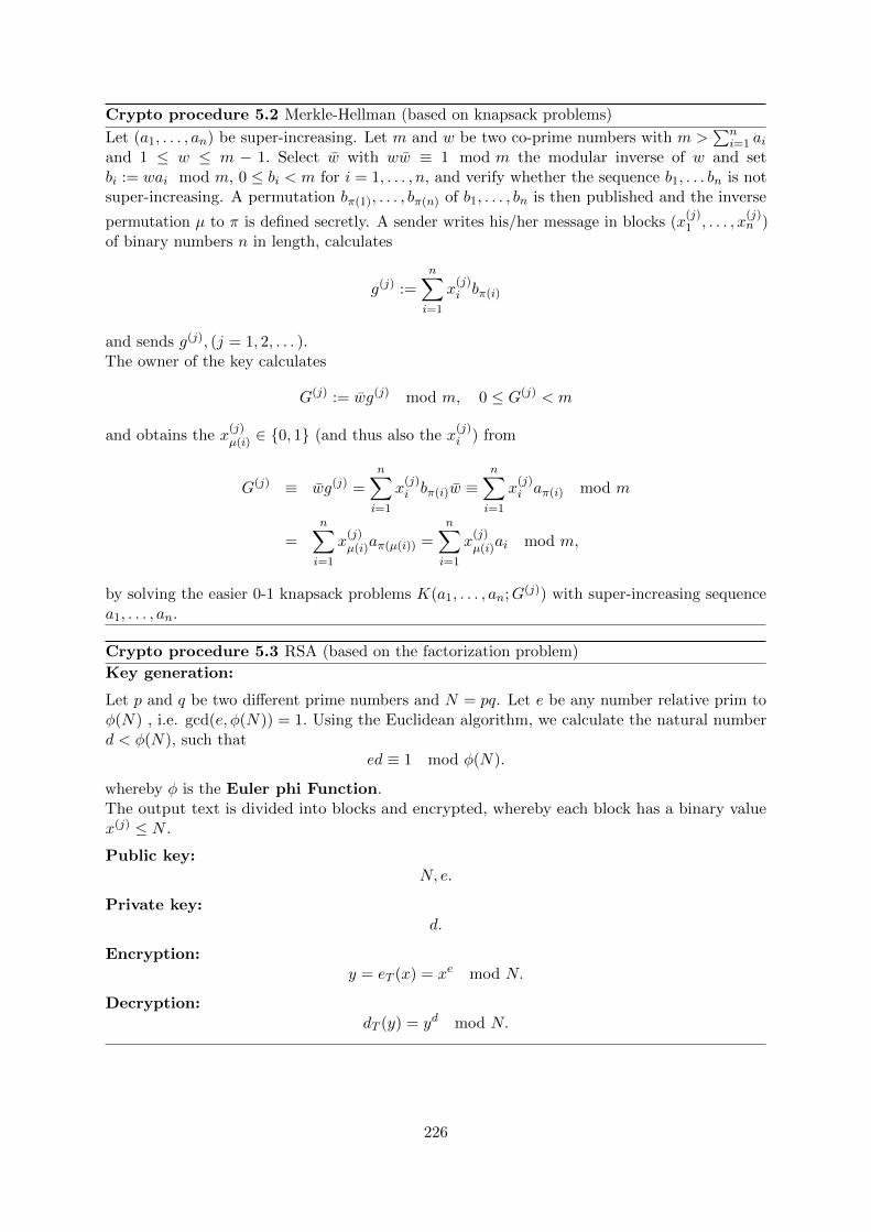
Crypto procedure 5.2 Merkle-Hellman (based on knapsack problems)
Let (a1, . . . , an) be super-increasing. Let m and w be two co-prime numbers with m >∑n
i=1 aiand 1 ≤ w ≤ m − 1. Select w with ww ≡ 1 mod m the modular inverse of w and setbi := wai mod m, 0 ≤ bi < m for i = 1, . . . , n, and verify whether the sequence b1, . . . bn is notsuper-increasing. A permutation bπ(1), . . . , bπ(n) of b1, . . . , bn is then published and the inverse
permutation µ to π is defined secretly. A sender writes his/her message in blocks (x(j)1 , . . . , x
(j)n )
of binary numbers n in length, calculates
g(j) :=n∑i=1
x(j)i bπ(i)
and sends g(j), (j = 1, 2, . . . ).The owner of the key calculates
G(j) := wg(j) mod m, 0 ≤ G(j) < m
and obtains the x(j)µ(i) ∈ {0, 1} (and thus also the x
(j)i ) from
G(j) ≡ wg(j) =
n∑i=1
x(j)i bπ(i)w ≡
n∑i=1
x(j)i aπ(i) mod m
=n∑i=1
x(j)µ(i)aπ(µ(i)) =
n∑i=1
x(j)µ(i)ai mod m,
by solving the easier 0-1 knapsack problems K(a1, . . . , an;G(j)) with super-increasing sequencea1, . . . , an.
Crypto procedure 5.3 RSA (based on the factorization problem)
Key generation:
Let p and q be two different prime numbers and N = pq. Let e be any number relative prim toφ(N) , i.e. gcd(e, φ(N)) = 1. Using the Euclidean algorithm, we calculate the natural numberd < φ(N), such that
ed ≡ 1 mod φ(N).
whereby φ is the Euler phi Function.The output text is divided into blocks and encrypted, whereby each block has a binary valuex(j) ≤ N .
Public key:N, e.
Private key:d.
Encryption:y = eT (x) = xe mod N.
Decryption:dT (y) = yd mod N.
226

Comment: Euler phi function
The Euler phi function is defined as:
φ(n) is the number of natural numbers x < nthat do not have a common factor with n.
No common factor means: Two natural numbers a and b are co-prime if gcd(a, b) = 1.
For the Euler phi function it holds that:
φ(1) = 1, φ(2) = 1, φ(3) = 2, φ(4) = 2, φ(6) = 2, φ(10) = 4, φ(15) = 8.
For example, φ(24) = 8, because
|{x < 24 : gcd(x, 24) = 1}| = |{1, 5, 7, 11, 13, 17, 19, 23}|.
Table 5.1 shows values of φ(n) up to n = 25.
n φ(n) The natural numbers that are co-prime to n and less than n.
1 1 12 1 13 2 1, 24 2 1, 35 4 1, 2, 3, 46 2 1, 57 6 1, 2, 3, 4, 5, 68 4 1, 3, 5, 79 6 1, 2, 4, 5, 7, 810 4 1, 3, 7, 915 8 1, 2, 4, 7, 8, 11, 13, 1420 8 1, 3, 7, 9, 11, 13, 17, 1925 20 1, 2, 3, 4, 6, 7, 8, 9, 11, 12, 13, 14, 16, 17, 18, 19, 21, 22, 23, 24
Table 5.1: Euler phi function
If p is a prime number, then φ(p) = p− 1.
In the case of N = pq:
φ(N) = pq(1− 1/p)(1− 1/q) = p(1− 1/p)q(1− 1/q) = (p− 1)(q − 1).
If we know the various prime factors p1, . . . , pk of n, then
φ(n) = n · (1− 1
p1) · · · (1− 1
pk).6
6Further formulas for the Euler phi function are in chapter 4.8.2 “The Euler phi function”.
227

The function eT is a one way function whose trapdoor information is the decomposition intoprimes of N .
At the moment, no algorithm is known that can factorize two prime numbers sufficientlyquickly for extremely large values (e.g. for several hundred decimal places). The quickest algo-rithms known today [Sti06] factorize a compound whole number N in a time period proportional
to L(N) = e√
ln(N) ln(ln(N)). Some example values can be found in table 5.2.
N 1050 10100 10150 10200 10250 10300
L(N) 1.42 · 1010 2.34 · 1015 3.26 · 1019 1.20 · 1023 1.86 · 1026 1.53 · 1029
Table 5.2: L(N) value table [factorization effort related to the modul length]
To this date, it has not been proved that the problem of breaking RSA is equivalent to thefactorization problem. Nevertheless, it is clear that the RSA procedure will no longer be safe ifthe factorization problem is “solved”.7
5.3.2 Rabin public key procedure (1979)
The Rabin public key procedure (crypto procedure 5.4) has been shown to be equivalent tobreaking the factorization problem. Unfortunately, this procedure is susceptible to chosen-ciphertext attacks.
Crypto procedure 5.4 Rabin (based on the factorization problem)
Let p and q be two different prime numbers with p, q ≡ 3 mod 4 and n = pq. Let 0 ≤ B ≤ n− 1.Public key:
e = (n,B).
Private key:d = (p, q).
Encryption:y = eT (x) = x(x+B) mod n.
Decryption:dT (y) =
√y +B2/4−B/2 mod n.
Caution: Because p, q ≡ 3 mod 4 the encryption is easy to calculate (if the key is known).This is not the case for p ≡ 1 mod 4. In addition, the encryption function is not injective: Thereare precisely four different source codes that have eT (x) as inverse image: x,−x − B,ω(x +B/2)−B/2,−ω(x+B/2)−B/2, where ω is one of the four roots of unity. The source codestherefore must be redundant for the encryption to remain unique!
Backdoor information is the decomposition into prime numbers of n = pq.
7In 2000 the authors assumed that values of the order magnitude 100 to 200 decimal places are currently safe.They estimates that the current computer technology indicates that a number with 100 decimal places could befactorized in approximately two weeks at justifiable costs, and using an expensive configuration (e.g. of around 10million US dollars), a number with 150 decimal places could be factorized in about a year, and a 200-digit numbershould remain impossible to factorize for a long time to come, unless there is a mathematical breakthrough.However, you can never be sure that there won’t be a mathematical breakthrough tomorrow.How easy it is to guess the future wrong is shown by the factorization of RSA-200 (see chapter 4.11.4) – completelywithout a “mathematical breakthrough”.
228

5.4 The discrete logarithm as basis for public key procedures8
Discrete logarithms form the basis for a large number of algorithms for public-key procedures.
5.4.1 The discrete logarithm in Zp
Let p be a prime number and let g ∈ Z∗p = {0, 1, . . . , p − 1}. Then the discrete exponentialfunction base g is defined as
eg : k −→ y := gk mod p, 1 ≤ k ≤ p− 1.
The inverse function is called a discrete logarithm function logg; the following holds:
logg(gk) = k.
The problem of the discrete logarithm (in Z∗p) is understood to be as follows:
Given p, g and y, determine k such that y = gk mod p.
It is much more difficult to calculate the discrete logarithm than to evaluate the discreteexponential function (see chapter 4.9). Table 5.3 lists several procedures for calculating thediscrete logarithm and their complexity [Sti06].
Name Complexity
Baby-step-giant-step O(√p)
Silver-Pohlig-Hellman polynomial in q, the greatestprime factor of p− 1.
Index-Calculus O(e(1+o(1))√
ln(p) ln(ln(p)))
Table 5.3: Procedures for calculating the discrete logarithm over Z∗p
The current record (as of April 2007) for calculating discrete logarithms was established inFebruary 2007 by the group Kleinjung, Franke and Bahr at University of Bonn.9 Kleinjungcalculated the discrete logarithm modulo a 160 digit prime number p and generator g:
p= b10159πc+ 119849= 314159265358979323846264338327950288419716939937510582097494
4592307816406286208998628034825342117067982148086513282306647093844609550582231725359408128481237299
g = 2
8With the educational tool for number theory NT you can play with the distribution of the discrete logarithmvalues and apply Shank’s baby-step-giant-step method: See learning units 6.1-6.3, pages 1-6/6.NT can be called in CT1 via the menu path Indiv. Procedures \ Number Theory Interactive \ LearningTool for Number Theory. See appendix A.6.
9http://www.nabble.com/Discrete-logarithms-in-GF(p)-----160-digits-t3175622.html
229

The discrete logarithms k of the following integer y was determined:10
y = b10159ec= 271828182845904523536028747135266249775724709369995957496696
7627724076630353547594571382178525166427427466391932003059921817413596629043572900334295260595630738
k = logg(y) mod p
= 829897164650348970518646802640757844024961469323126472198531845186895984026448342666252850466126881437617381653942624307537679319636711561053526082423513665596
The search was performed with GNFS method (general number field sieve, Index-Calculus) andtook about 17 CPU years on 3.2 GHz Xeon machines.
5.4.2 Diffie-Hellman key agreement11
The mechanisms and algorithms of classical cryptography only take effect when the subscribershave already exchanged the secret key. In classical cryptography you cannot avoid exchang-ing secrets without encrypting them. Transmission safety here must be achieved using non-cryptographic methods. We say that we need a secret channel for exchanging secrets. Thischannel can be realised either physically or organisationally.What is revolutionary about modern cryptography is, amongst other things, that you no longerneed secret channels: You can agree secret keys using non-secret, i.e. public channels.One protocol that solves this problem is that of Diffie and Hellman (crypto procedure 5.5).
Crypto procedure 5.5 Diffie-Hellman key agreement
Two subscribers A and B want to agree on a joint secret key.Let p be a prime number and g a natural number. These two numbers do not need to be secret.The two subscribers then select a secret number a and b from which they calculate the valuesα = ga mod p and β = gb mod p. They then exchange the numbers α and β. To end with, thetwo subscribers calculate the received value to the power of their secret value to get βa mod pand αb mod p.Thus
βa ≡ (gb)a ≡ gba ≡ gab ≡ (ga)b ≡ αb mod p
The safety of the Diffie-Hellman protocol is closely connected to calculating the discretelogarithm mod p. It is even thought that these problems are equivalent.
5.4.3 ElGamal public key encryption procedure in Z∗p
By varying the Diffie-Hellman key agreement protocol slightly, you can obtain an asymmetricencryption algorithm, crypto procedure 5.6. This observation was made by Taher ElGamal.
10The integer y was chosen as the first 159 digits of the Euler number e.11With CT1 this exchange protocol has been visualized: you can execute the single steps with concrete numbers
using menu Indiv. Procedures \ Protocols \ Diffie-Hellman Demonstration.In JCT you can find it in the default perspective via the menu item Visuals \ Diffie-Hellman Key Exchange(EC).
230

Crypto procedure 5.6 ElGamal (based on the discrete logarithm problem)
Let p be a prime number such that the discrete logarithm in Zp is difficult to compute. Letα ∈ Z∗p be a primitive element. Let a ∈ IN and β = αa mod p.Public key:
p, α, β.
Private key:a.
Let k ∈ Zp−1 be a random number and x ∈ Z∗p the plaintext.Encryption:
eT (x, k) = (y1, y2),
wherey1 = αk mod p
andy2 = xβk mod p.
Decryption:dT (y1, y2) = y2(y
a1)−1 mod p
5.4.4 Generalized ElGamal public key encryption procedure
The discrete logarithm can be generalized in any number of finite groups (G, ◦). The followingprovides several properties of G, that make the discrete logarithm problem difficult. Instead ofg ◦ h we often write only gh.
Calculating the discrete exponential function Let G be a group with the operation ◦and g ∈ G. The (discrete) exponential function base g is defined as
eg : k 7−→ gk, for all k ∈ N.
wheregk := g ◦ . . . ◦ g︸ ︷︷ ︸
k times
.
The exponential function is easy to calculate:
Lemma. The power gk can be calculated in at most 2 log2 k group operations.
ProofLet k = 2n+kn−12n−1+· · ·+k12+k0 be the binary representation of k. Then n ≤ log2(k), because2n ≤ k < 2n+1. k can be written in the form k = 2k′ + k0 with k′ = 2n−1 + kn−12
n−2 + · · ·+ k1.Thus
gk = g2k′+k0 = (gk
′)2gk0 .
We therefore obtain gk from gk′
by squaring and then multiplying by g. The claim is thus provedby induction to n. 2
Problem of the discrete logarithm
231

Let G by a finite group with the operation ◦. Let α ∈ G andβ ∈ H = {αi : i ≥ 0}.We need to find a unique a ∈ N with 0 ≤ a ≤ |H| − 1 and β = αa.We define a as logα(β).
Calculating the discrete logarithm A simple procedure for calculating the discrete loga-rithm of a group element, that is considerably more efficient than simply trying all possiblevalues for k, is the baby-step-giant-step algorithm.
Theorem 5.4.1. [baby-step-giant-step algorithm] Let G be a group and g ∈ G. Let n be thesmallest natural number with |G| ≤ n2. Then the discrete logarithm of an element h ∈ G can becalculated base g by generating the following two lists each containing n elements and comparingthese lists:
giant-step list: {1, gn, g2n, . . . , gn·n},baby-step list: {hg−1, hg−2, . . . , hg−n}.
After detecting a common element the calculation can be stopped. In order to calculate theselists, we need 2n group operations.
ProofIf gjn = hg−i, i.e. h = gi+jn, then the problem is solved. If the lists are disjoint, then h cannotbe represented as gi+jn, i, j ≤ n,. As all powers of g are thus recorded, the logarithm problemdoes not have a solution. 2
You can use the baby-step-giant-step algorithm to demonstrate that it is much more difficultto calculate the discrete logarithm than to calculate the discrete exponential function. If thenumbers that occur have approximately 1000 bits in length, then you only need around 2000multiplications (see theorem 5.4.1) to calculate all gk, but around 2500 ≈ 10150 operations tocalculate the discrete logarithm using the baby-step-giant-step algorithm.In addition to the baby-step-giant-step algorithm, there are also numerous other procedures forcalculating the discrete logarithm [Sti06].
The theorem from Silver-Pohlig-Hellman In finite Abelian groups, the discrete logarithmproblem can be reduced to groups of a lower order.
Theorem 5.4.2. [Silver-Pohlig-Hellman] Let G be a finite Abelian group with |G| = pa11 pa22 · . . . ·
pass . The discrete logarithm in G can then be reduced to solving logarithm problems in groups ofthe order p1, . . . , ps.
If |G| contains a “dominant” prime factor p, then the complexity of the logarithm problem isapproximately
O(√p).
Therefore, if the logarithm problem is to be made difficult, the order of the group used G shouldhave a large prime factor. In particular, if the discrete exponential function in the group Z∗p isto be a one way function, then p− 1 must be a large prime factor. In this case a generalizedElGamal procedure can be defined (crypto procedure 5.7).
232
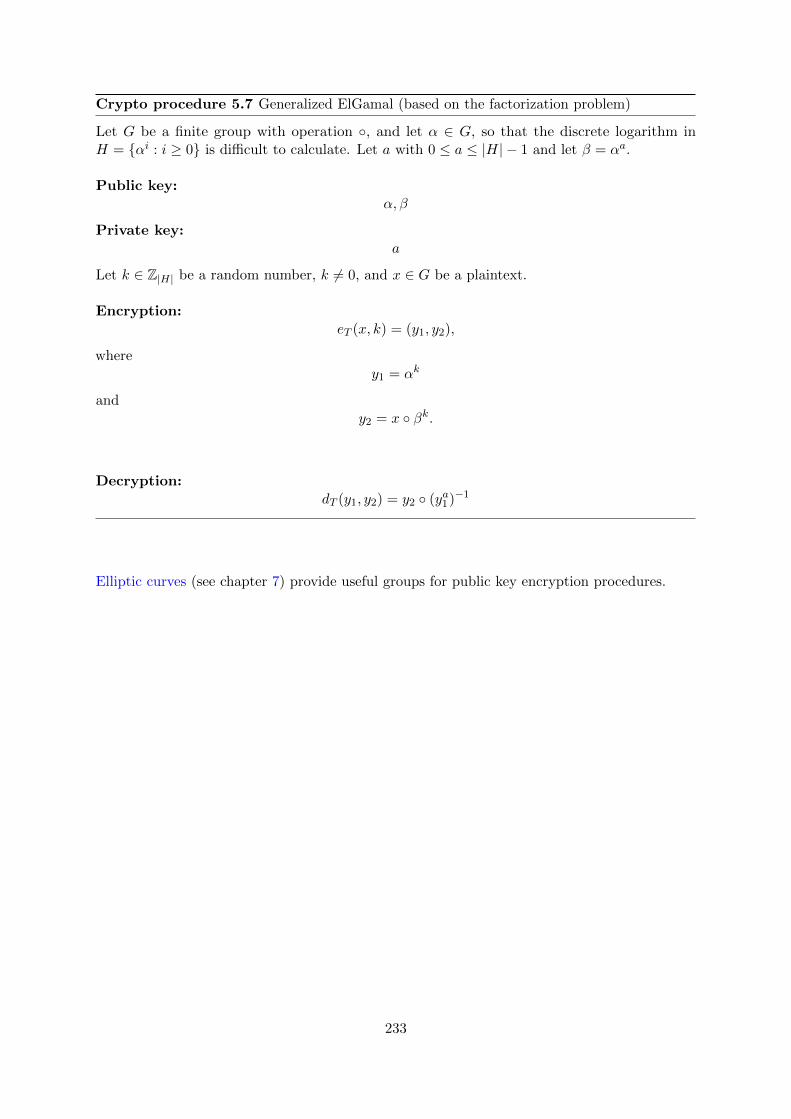
Crypto procedure 5.7 Generalized ElGamal (based on the factorization problem)
Let G be a finite group with operation ◦, and let α ∈ G, so that the discrete logarithm inH = {αi : i ≥ 0} is difficult to calculate. Let a with 0 ≤ a ≤ |H| − 1 and let β = αa.
Public key:α, β
Private key:a
Let k ∈ Z|H| be a random number, k 6= 0, and x ∈ G be a plaintext.
Encryption:eT (x, k) = (y1, y2),
wherey1 = αk
andy2 = x ◦ βk.
Decryption:dT (y1, y2) = y2 ◦ (ya1)−1
Elliptic curves (see chapter 7) provide useful groups for public key encryption procedures.
233

Bibliography (Chap ModernCrypto)
[Adl83] Adleman, L.: On breaking the iterated Merkle-Hellman public-key Cryptosystem. InAdvances in Cryptologie, Proceedings of Crypto 82, pages 303–308. Plenum Press, 1983.
[BDG98] Balcazar, J. L., J. Daaz, and J. Gabarr: Structural Complexity I. Springer, 1998.
[Bri85] Brickell, E. F.: Breaking Iterated Knapsacks. In Advances in Cryptology: Proc.CRYPTO’84, Lecture Notes in Computer Science, vol. 196, pages 342–358. Springer,1985.
[Hes01] Hesselink, Wim H.: The borderline between P and NP, February 2001. http://www.
cs.rug.nl/~wim/pub/whh237.pdf.
[Lag83] Lagarias, J. C.: Knapsack public key Cryptosystems and diophantine Approximation.In Advances in Cryptology, Proceedings of Crypto 83. Plenum Press, 1983.
[MH78] Merkle, R. and M. Hellman: Hiding information and signatures in trapdoor knapsacks.IEEE Trans. Information Theory, IT-24, 24, 1978.
[RSA78] Rivest, Ron L., Adi Shamir, and Leonard Adleman: A Method for Obtaining DigitalSignatures and Public-Key Cryptosystems. Communications of the ACM, 21(2):120–126,April 1978.
[Sha82] Shamir, A.: A polynomial time algorithm for breaking the basic Merkle-Hellman Cryp-tosystem. In Symposium on Foundations of Computer Science, pages 145–152, 1982.
[Sti06] Stinson, Douglas R.: Cryptography – Theory and Practice. Chapman & Hall/CRC,3rd edition, 2006.
All links have been confirmed at July 13, 2016.
234

Chapter 6
Hash Functions and DigitalSignatures
(Joerg-Cornelius Schneider / Bernhard Esslinger / Henrik Koy, Jun 2002; Updates: Feb 2003,Jun 2005, Jul 2009, Nov 2012)
We can make everything out of this world, but we cannot create a world, where humans in someten thousand years can think: ’Ok, now it is enough. Everything should stay like it is. Let’s dono changes any more, don’t do inventions any more, because it cannot become better, and if,
then we don’t want this.’
Quote 16: Stanislaw Lem1
The aim of digital signatures is to guarantee the following two points:
• User authenticity:It can be checked whether a message really does come from a particular person.
• Message integrity:It can be checked whether the message has been changed (on route).
An asymmetric technique is used again (see encryption procedures). Participants who wishto generate a digital signature for a document must possess a pair of keys. They use their secretkey to generate signatures and the recipient uses the sender’s public key to verify whether thesignature is correct. As before, it must be impossible to use the public key to derive the secretkey.
In detail, a Signature procedure2 looks like this:Senders use their message and secret key to calculate the digital signature for the message.Compared to hand-written signatures, digital signatures therefore have the advantage that theyalso depend on the document to be signed. Signatures from one and the same participant aredifferent unless the signed documents are completely identical. Even inserting a blank in the
1This was the answer of Stanislaw Lem to heavy critics at his philosophical main book “Summa Technologiae”,1964, where he thought about the possibility of an evolution creating artificial intelligence.
2With CT1 you can also generate and check digital signatures: Usingthe submenus of the main menu Digital Signatures / PKI or usingmenu Indiv. Procedures \ RSA Cryptosystem \ Signature Demonstration (Signature Generation).Also with JCT (in the default and the algorithm perspektive) its possible to create different kinds of electronicsignatures.
235
text would lead to a different signature. The recipient of the message would therefore detect anyinjury to the message integrity as this would mean that the signature no longer matches thedocument and is shown to be incorrect when verified.
The document is sent to the recipient together with the signature. The recipient can then usethe sender’s public key, the document and the signature to establish whether or not the signatureis correct. The procedure we just described has in practice, however, a decisive disadvantage.The signature would be approximately as long as the document itself. To prevent an unnecessaryincrease in data traffic, and also for reasons of performance, we apply a cryptographic hashfunction3 to the document – before signing. The output of the hash function will then be signed.
6.1 Hash functions
A hash function4 maps a message of any length to a string of characters with a constant size,the hash value.
6.1.1 Requirements for hash functions
Cryptographically secure hash functions fulfill the following three requirements (the order is in away that the requirements increase):
• Resistance against 1st pre-image attacks:It should be practically impossible, for a given number, to find a message that has preciselythis number as hash value.Given (fix): hash value H’,Searched: message m, so that: H(m) = H’.
• Resistance against 2nd pre-image attacks:It should be practically impossible, for a given message, to find another message, whichhas precisely the same hash value.Given (fix): message m1 [and so the hash value H1 = H(m1)],Searched: message m2, so that: H(m2) = H1.
• Collision resistance:It should be practically impossible to find any two messages with the same hash value (it
3Hash functions are implemented within CT1 at several places.Using menus Individual Procedures \ Hash and Analysis \ Hash you have the possibilities
• to apply one of 6 hash functions to the content of the current window,
• to calculate the hash value of a file,
• to test, how changes to a text change the according hash value,
• to calculate a key from a password according to the PKCS#5 standard,
• to calculate HMACs from a text and a secret key, and
• to perform a simulation, how digital signatures could be attacked by a targeted search for hash value collisions.
CT2 and JCT also contain different hash methods: See the functions’ lists within the appendix A.2 and A.3.4Hash algorithms compute a condensed representation of electronic data (message). When a message is input to ahash algorithm, the result is an output called a message digest. The message digests typically range in length from128 to 512 bits, depending on the algorithm. Secure hash algorithms are typically used with other cryptographicalgorithms, such as digital signature algorithms and keyed-hash message authentication codes, or in the generationof random numbers (bits).
236

doesn’t matter what hash value).Searched: 2 messages m1 and m2, so that: H(m1) = H(m2).
6.1.2 Current attacks against hash functions // SHA-3
So far, no formal proof has been found that perfectly secure cryptographic hash functions exist.
During the past several years no new attacks against hash algorithms came up, and so thecandidates that had not yet shown any weaknesses in their structure in practice (e.g. SHA–15 orRIPEMD-1606) were trusted.
At Crypto 2004 (August 2004)7 this safety-feeling was disputed: Chinese researchers publishedcollision attacks against MD4, SHA-0 and parts of SHA-1. This globally caused new motivationto engage in new hash attack methods.
The initially published result reduced the expected complexity for one SHA-1 collision searchfrom 280 (brute-force) to 269 [WYY05b]. More recent announcements claim to further reducethe required effort to 263 [WYY05a] and 252 [MHP12]. This would bring collision attacks intothe practical realm, as similar efforts have been mastered in the past (s. 1.3.3).
According to our current knowledge there is no need to run scared. But in the future digitalsignatures should use longer hash values and/or other hash algorithms.
Already before Crypto 2004 the U.S. National Institute of Standards and Technology (NIST)announced, to discontinue SHA-1 in the next few years. So it is recommended not to use SHA-1for new products generating digital signatures. The SHA-2 family [NIS15] provides strongeralgorithms.
To address new findings in cryptanalysis, in 2008 NIST opened a competition to developa new cryptographic hash algorithm beyound the SHA-2 family: In October 2012 Keccak wasannounced as “SHA-3”.8
5SHA-1 is a 160 bit hash function specified in FIPS 180-1 (by NIST), ANSI X9.30 Part 2 and [NIS13].SHA means Secure Hash Algorithm, and is widely used, e.g. with DSA, RSA or ECDSA.The current standard [NIS15] defines four secure hash algorithms – SHA-1, SHA-256, SHA-384, and SHA-512.For these hash algorithms there are also validation tests defined in the test suite FIPS 140-2.
The output length of the SHA algorithms was enhanced because of the possibility of birthday attacks: thesemake n-bit AES and a 2n-bit hash roughly equivalent:- 128-bit AES – SHA-256- 192-bit AES – SHA-384- 256-bit AES – SHA-512.
With CT1 you can comprehend the birthday attack on digital signatures:using the menu Analysis \ Hash \ Attack on the Hash Value of the Digital Signature.CT2 contains an MD5 collider.
6RIPEMD-160, RIPEMD-128 and the optional extension RIPEMD-256 have object identifiers defined by theISO-identified organization TeleTrusT, both as hash algorithm and in combination with RSA. RIPEMD-160 isalso part of the ISO/IEC international standard ISO/IEC 10118-3:1998 on dedicated hash functions, togetherwith RIPEMD-128 and SHA-1. Further details:- http://www.esat.kuleuven.ac.be/~bosselae/ripemd160.html- http://www.ietf.org/rfc/rfc2857.txt (“The Use of HMAC-RIPEMD-160-96 within ESP and AH”).7http://www.iacr.org/conferences/crypto2004/8http://csrc.nist.gov/groups/ST/hash/sha-3/
With CT2 you can execute and visualize the Keccak hash function – using in the Startcenter Templates \ HashFunctions \ Keccak Hash (SHA-3).Keccak also can be used as pseudo random number generator and as stream cipher: This can be found within theStartcenter templates via Tools \ Keccak PRNG, and Cryptography \ Modern Ciphers \ Symmetric\ Keccak Streamcipher.
237
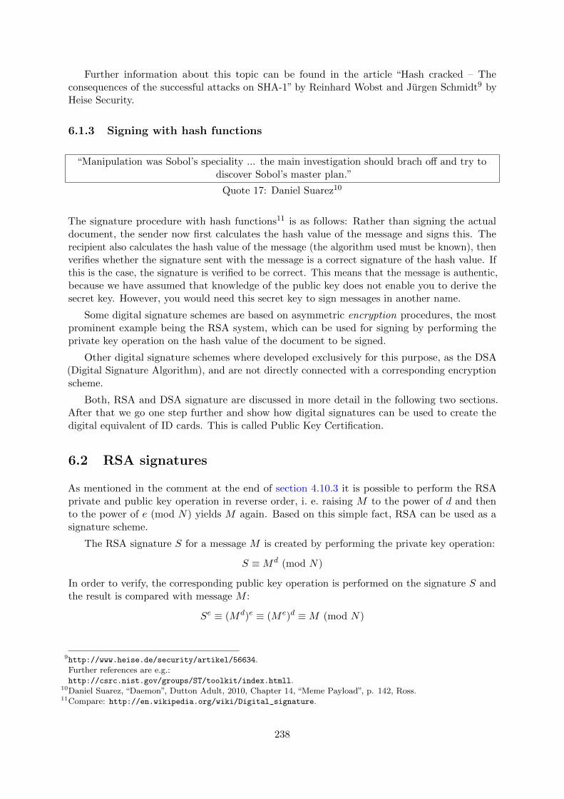
Further information about this topic can be found in the article “Hash cracked – Theconsequences of the successful attacks on SHA-1” by Reinhard Wobst and Jurgen Schmidt9 byHeise Security.
6.1.3 Signing with hash functions
“Manipulation was Sobol’s speciality ... the main investigation should brach off and try todiscover Sobol’s master plan.”
Quote 17: Daniel Suarez10
The signature procedure with hash functions11 is as follows: Rather than signing the actualdocument, the sender now first calculates the hash value of the message and signs this. Therecipient also calculates the hash value of the message (the algorithm used must be known), thenverifies whether the signature sent with the message is a correct signature of the hash value. Ifthis is the case, the signature is verified to be correct. This means that the message is authentic,because we have assumed that knowledge of the public key does not enable you to derive thesecret key. However, you would need this secret key to sign messages in another name.
Some digital signature schemes are based on asymmetric encryption procedures, the mostprominent example being the RSA system, which can be used for signing by performing theprivate key operation on the hash value of the document to be signed.
Other digital signature schemes where developed exclusively for this purpose, as the DSA(Digital Signature Algorithm), and are not directly connected with a corresponding encryptionscheme.
Both, RSA and DSA signature are discussed in more detail in the following two sections.After that we go one step further and show how digital signatures can be used to create thedigital equivalent of ID cards. This is called Public Key Certification.
6.2 RSA signatures
As mentioned in the comment at the end of section 4.10.3 it is possible to perform the RSAprivate and public key operation in reverse order, i. e. raising M to the power of d and thento the power of e (mod N) yields M again. Based on this simple fact, RSA can be used as asignature scheme.
The RSA signature S for a message M is created by performing the private key operation:
S ≡Md (mod N)
In order to verify, the corresponding public key operation is performed on the signature S andthe result is compared with message M :
Se ≡ (Md)e ≡ (M e)d ≡M (mod N)
9http://www.heise.de/security/artikel/56634.Further references are e.g.:http://csrc.nist.gov/groups/ST/toolkit/index.htmll.
10Daniel Suarez, “Daemon”, Dutton Adult, 2010, Chapter 14, “Meme Payload”, p. 142, Ross.11Compare: http://en.wikipedia.org/wiki/Digital_signature.
238
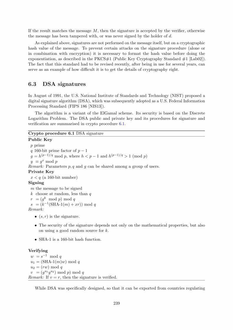
If the result matches the message M , then the signature is accepted by the verifier, otherwisethe message has been tampered with, or was never signed by the holder of d.
As explained above, signatures are not performed on the message itself, but on a cryptographichash value of the message. To prevent certain attacks on the signature procedure (alone orin combination with encryption) it is necessary to format the hash value before doing theexponentiation, as described in the PKCS#1 (Public Key Cryptography Standard #1 [Lab02]).The fact that this standard had to be revised recently, after being in use for several years, canserve as an example of how difficult it is to get the details of cryptography right.
6.3 DSA signatures
In August of 1991, the U.S. National Institute of Standards and Technology (NIST) proposed adigital signature algorithm (DSA), which was subsequently adopted as a U.S. Federal InformationProcessing Standard (FIPS 186 [NIS13]).
The algorithm is a variant of the ElGamal scheme. Its security is based on the DiscreteLogarithm Problem. The DSA public and private key and its procedures for signature andverification are summarised in crypto procedure 6.1.
Crypto procedure 6.1 DSA signature
Public Key
p primeq 160-bit prime factor of p− 1
g = h(p−1)/q mod p, where h < p− 1 and h(p−1)/q > 1 (mod p)y ≡ gx mod p
Remark: Parameters p, q and g can be shared among a group of users.Private Key
x < q (a 160-bit number)Signing
m the message to be signedk choose at random, less than qr = (gk mod p) mod qs = (k−1(SHA-1(m) + xr)) mod q
Remark:
• (s, r) is the signature.
• The security of the signature depends not only on the mathematical properties, but alsoon using a good random source for k.
• SHA-1 is a 160-bit hash function.
Verifying
w = s−1 mod qu1 = (SHA-1(m)w) mod qu2 = (rw) mod qv = (gu1yu2) mod p) mod q
Remark: If v = r, then the signature is verified.
While DSA was specifically designed, so that it can be exported from countries regulating
239
export of encryption soft and hardware (like the U.S. at the time when it was specified), it hasbeen noted [Sch96, p. 490], that the operations involved in DSA can be used to emulate RSAand ElGamal encryption.
6.4 Public key certification
The aim of public key certification is to guarantee the connection between a public key and auser and to make it traceable for external parties. In cases in which it is impossible to ensurethat a public key really belongs to a particular person, many protocols are no longer secure,even if the individual cryptographic modules cannot be broken.
6.4.1 Impersonation attacks
Assume Charlie has two pairs of keys (PK1, SK1) and (PK2, SK2), where SK denotes the secretkey and PK the public key. Further assume that he manages to palm off PK1 on Alice as Bob’spublic key and PK2 on Bob as Alice’s public key (by falsifying a public key directory).
Then he can attack as follows:
• Alice wants to send a message to Bob. She encrypts it using PK1 because she thinks thatthis is Bob’s public key. She then signs the message using her secret key and sends it.
• Charlie intercepts the message, removes the signature and decrypts the message using SK1.If he wants to, he can then change the message in any way he likes. He then encrypts themessage again, but this time using Bob’s genuine public key, which he has taken from apublic key directory, signs the message using SK2 and forwards it to Bob.
• Bob verifies the signature using PK2 and will reach the conclusion that the signature iscorrect. He then decrypts the message using his secret key.
In this way Charlie can listen in on communication between Alice and Bob and change theexchanged messages without them noticing. The attack will also work if Charlie only has onepair of keys.
Another name for this type of attack is “man-in-the-middle attack”. Users are promisedprotection against this type of attack by public-key certification, which is intended to guaranteethe authenticity of public keys. The most common certification method is the X.509 standard.
6.4.2 X.509 certificate
Each participant who wants to have an X.509 certificate ([IT97]) verifying that his public keybelongs to a real person consults what is known as a certification authority (CA)12. He proveshis identity to this CA (for example by showing his ID). The CA then issues him an electronicdocument (certificate) which essentially contains the name of the certificate-holder and the nameof the CA, the certificate-holder’s public key and the validity period of the certificate. The CAthen signs the certificate using its secret key.
Anyone can now use the CA’s public key to verify whether a certificate is falsified. The CAtherefore guarantees that a public key belongs to a particular user.
12Often called trust center, if the certificates are not only offered to a closed user group.
240

This procedure is only secure as long as it can be guaranteed that the CA’s public key iscorrect. For this reason, each CA has its public key certified by another CA that is superior inthe hierarchy. In the upper hierarchy level there is usually only one CA, which can of coursethen have its key certified by another CA. It must therefore transfer its key securely in anotherway. In the case of many software products that work with certificates (such as the Microsoftand Netscape Web browsers), the certificates of these root CAs are permanently embedded inthe program right from the start and cannot be changed by users at a later stage. However,(public) CA keys, in particularly those of the root entity, can also be secured by means of makingthem available publicly.
241
Bibliography (Chap DigSig)
[IT97] ITU-T: ITU-T Recommendation X.509 (1997 E): Information Technology – OpenSystems Interconnection – The Directory: Authentication Framework. Technicalreport, International Telecommunication Union ITU-T, June 1997.
[Lab02] Labs, RSA: PKCS #1 v2.1 Draft 3: RSA Cryptography Standard. Technical report,RSA Laboratories, April 2002.
[MHP12] McDonald, Cameron, Philip Hawkes, and Josef Pieprzyk: Differential Path for SHA-1with complexity O(252). Cryptology ePrint Archive, 2012. http://eprint.iacr.org/2009/259.
[NIS13] NIST: Digital Signature Standard (DSS). Technical report, NIST (U.S. Departmentof Commerce), 2013. Change note 4.http://nvlpubs.nist.gov/nistpubs/FIPS/NIST.FIPS.186-4.pdf,http://csrc.nist.gov/publications/PubsFIPS.html.
[NIS15] NIST: Secure Hash Standard (SHS). Technical report, NIST (U.S. Department ofCommerce), August 2015. FIPS 180-4 supersedes FIPS 180-2.http://nvlpubs.nist.gov/nistpubs/FIPS/NIST.FIPS.180-4.pdf,http://csrc.nist.gov/publications/PubsFIPS.html.
[Sch96] Schneier, Bruce: Applied Cryptography, Protocols, Algorithms, and Source Code inC. Wiley, 2nd edition, 1996.
[WYY05a] Wang, Xiaoyun, Andrew Yao, and Frances Yao: New Collision Search for SHA-1.Technical report, Crypto 2005, Rump Session, 2005.http://www.iacr.org/conferences/crypto2005/rumpSchedule.html.
[WYY05b] Wang, Xiaoyun, Yiqun Yin, and Hongbo Yu: Finding Collisions in the Full SHA-1.Advances in Cryptology-Crypto, LNCS 3621, pages 17–36, 2005.
All links have been confirmed at July 14, 2016.
242

Chapter 7
Elliptic Curves
(Bartol Filipovic / Matthias Bueger / Bernhard Esslinger / Roger Oyono, Apr 2000, Updates:Dec 2001, Jun 2002, Mar 2003, Nov 2009, Aug 2013, Aug 2016)
7.1 Elliptic-curve cryptography – a high-performance substi-tute for RSA?
In many business sectors secure and efficient data transfer is essential. In particular, the RSAalgorithm is used in many applications. Although the security of RSA is beyond doubt, theevolution in computing power has caused a growth in the necessary key length. Today, 1024-bitRSA keys are standard, but the GISA (German Information Security Agency) recommends theusage of 2048-bit keys from 2006 on (compare section 4.11). The fact that most chips on smartcards cannot process keys extending ca. 2000 bit shows that there is a need for alternatives inthe area of asymmetric cryptography. Elliptic-curve cryptography (ECC) is such an alternative.They are used widely on smartcards.
The efficiency of a cryptographic algorithm depends on the key length and the calculationeffort that is necessary to provide a prescribed level of security. The major advantage of ECCcompared to RSA is that it requires much shorter key lengths.
If we assume that the computing power increases by Moore’s law (i. e. it doubles every 18months)1, then the evolution of the key lengths for secure communication will be as in figure 7.1,which was generated from table 1 (on page 32 in [LV01]).2
In addition, a digital signature can be processed 10-times faster with ECC than with RSA.However, verification of a given signature is still more efficient with RSA than with ECC. Referto figure 7.2 (source: J. Merkle, Elliptic-Curve Cryptography Workshop, 2001) for a comparison.The reason is that RSA public keys can be chosen relatively small as long as the secret key islong enough.
Nevertheless, thin clients like smart cards usually have to store the (long) secret key and
1Moore’s law formulates the empirical observation and the according forecast that the number of components ortransistors on an integrated circuit doubles every two years. It referred originally only to the transistors densityin an integrated circuit, however not, for example, to the increase in the storage density. This realization fortransistors density in 1965 (with a correction 1975) was expressed by Gordon Moore, a co-founder of Intel. Inrecent years, the growth of computing power was even higher than the forecasted doubling every 2 years. Futurelimits are set by the transistors size of a few atoms, which could be achieved by 2020.
2Further information about key length comparison by Arjen Lenstra und Eric Verheul, plus more modern evaluationstill 2015 can be found in the interactive website http://www.keylength.com.
243

Key
leng
th n
eede
d (b
its)
0
500
1000
1500
2000
2500
3000
3500
2010 2030 204020202000
ECC
RSA
Year
Figure 7.1: Prognosis of the key lengths regarded to be safe for RSA and for elliptic curves
have to process a digital signature rather than verify one. Therefore, there is a clear advantagein using ECC in terms of efficiency.
Nowadays, the major problem with ECC implementations is the lack of standardization.There is only one way to implement RSA, but there are many ways for ECC: One can workwith different sets of numbers, different (elliptic) curves — described by parameters3 — , anda variety of representations of the elements on the curve. Each choice has its advantages anddisadvantages, and one can certainly construct the most efficient for each application. However,this causes problems in interoperability. But if all ECC-tools should be able to communicate witheach other, they will have to support all different algorithms, which might put the advantage ofefficient computation and the need of less storage capacity to the contrary.
Therefore, international standardization organizations like IEEE (P1363), ASC (ANSI X9.62,X9.63), ISO/IEC as well as major players like RSA labs or Certicom have recently startedstandardization initiatives. While the IEEE only describes the different implementations, theASC has explicitly stated 10 elliptic curves and recommends their usage. The advantage of theASC approach is that one needs only a single byte to indicate which curve is meant. However, itis not yet clear whether the ASC curves will become a de facto standard.
Although there is no need to replace RSA in any application today4, one seriously shouldtake the usage of ECC into consideration5.GISA More current discussions about the security ofECC can be found in chapter 10.
7.2 Elliptic curves – history
Mathematicians have been researching elliptic curves for over 100 years. Over the course of time,many lengthy and mathematically complex results have been found and published which areconnected to elliptic curves. A mathematician would say that elliptic curves (or the mathematics
3See chapter 7.44Current information about the security of the RSA algorithm can be found in chapters 4.11 and 10.5Compare the technical guideline “Cryptographic Methods: Recommendations and Keylengths” of GISA fromFebruary 15th, 2016.
244

0
100
300
200
400
500
600
ECC 160 Bit RSA 1024 Bit
# 10
24−
bit m
ultip
licat
ions
Sign
Verify
Figure 7.2: Comparison between signing and verification time for RSA and elliptic curves
behind them) are widely understood. This research was originally purely mathematical. Thatis to say, elliptic curves were investigated, for example, in the mathematical areas of numbertheory and algebraic geometry, which are generally highly abstract. Even in the recent past,elliptic curves played an important role in pure mathematics. In 1993 and 19946 , Andrew Wilespublished mathematical works that triggered enthusiasm far beyond the specialist audience. Inthese works, he proved a conjecture put forward in the 1960’s. To put it short, this conjecturewas concerned with the connection between elliptic curves and what are called module forms.What is particularly interesting for most people is that the works of Wiles also proved the famoussecond theorem of Fermat. Mathematicians had spent centuries (Fermat lived from 1601 to1665) trying to find a strict proof of this theorem. Understandably, therefore, Wiles’ proof got agood response. Fermat formulated his theorem as follows (written in the borders of a book fromDiophantus):
Cubum autem in duos cubos, aut quadratoquadratum in duos quadratoquadratos, etgeneraliter nullam in infinitum ultra quadratum potestatem in duos ejusdem nominisfas est dividere: cujus rei demonstrationem mirabilem sane detexi. Hanc marginisexiguitas non caperet.
With a free translation, using the denotation of modern mathematics, this means:No positive whole numbers x, y and z greater than zero exist such that xn + yn = zn for n > 2.I have found an amazing proof of this fact, but there is too little space within the confines ofthis book to include it.
This is truly amazing: A statement that is relatively simple to understand (we are referringto Fermat’s second theorem here) could only be proved after such a long period of time, although
61994 the gaps in the first proof have been closed by Wiles and Richard Taylor.
245

Fermat himself claimed to have found a proof. What’s more, the proof found by Wiles isextremely extensive (all of Wiles publications connected with the proof made up a book inthemselves). This should therefore make it obvious that elliptic curves are generally based onhighly complex mathematics.
Anyway, that’s enough about the role of elliptic curves in pure mathematics. In 1985Neal Koblitz and Victor Miller independently suggested using elliptic curves in cryptography.Elliptic curves have thus also found a concrete practical application. Another interesting area ofapplication for elliptic curves is for factorizing whole numbers (the RSA cryptographic systemis based on the difficulty/complexity of finding prime factors of an extremely large number;compare section 4.11.). In this area, procedures based on elliptic curves have been investigatedand used since 1987 (compare section 7.8).There are also prime number tests based on elliptic curves.
Elliptic curves are used differently in the various areas: Encryption procedures based onelliptic curves are based on the difficulty of the problem known as elliptic curve discrete logarithm.The factorization of natural composite numbers n uses the fact that a large number of ellipticcurves can be generated for n.
7.3 Elliptic curves – mathematical basics
This section provides information about groups and fields.7
7.3.1 Groups
Because the term group is used differently in everyday language than in mathematics, we will,for reasons of completeness, begin by introducing the essential statement of the formal definitionof a group:
• A group is a non-empty set G on which an operation “·”. The set G is closed underthis operation, which means that for any two elements a, b taken from G, performing theoperation on them gives an element in G, i.e. ab = a · b lies in G.
• For all elements a, b and c in G: (ab)c = a(bc) (associative law).
• There exists an element e in G that behaves neutrally with respect to the operation ·.That means that for all a in the set G : ae = ea = a.
• For each element a in G there exists a so-called inverse8 element a−1 in G such that:aa−1 = a−1a = e.
If in addition it applies ab = ba (commutative law) for all a, b in G, then we call the groupan Abelian group.
Since we may define different operations on the same set, we distinguish them by givingthem different names (e.g. + addition or · multiplication).
The simplest example of an (Abelian) group is the group of whole numbers under the standardoperation of addition. The set of whole numbers is denoted as Z. Z has an infinite number of
7A didactically well prepared introduction into Elliptic Curves can be found in [SWE15].8The inverse is uniquely determined because if x, y ∈ G are each inverse to a, i.e. ax = xa = e and ay = ya = e,then x = xe = x(ay) = (xa)y = ey = y.
246
elements: Z = {· · · ,−4,−3,−2,−1, 0, 1, 2, 3, 4, · · · }. For example, the operation of 1 + 2 lies inZ, for 1 + 2 = 3 and 3 lies in Z. The neutral element in the group Z is 0. The inverse element of3 is −3, for 3 + (−3) = 0.
For our purpose, so-called finite groups play an important role. This means that there existsa set M with a fixed number of elements and an operation + such that the above conditions arefulfilled. One example is the group Zn = {0, 1, 2, 3, · · · , n− 1} of the remainders of the divisionby n ∈ N, and the operation is an addition mod n. So, for example, a and b in Zn are subject tothe operation a+ b mod n.
Cyclic groups Cyclic groups9 are those groups G′ that possess an element g from whichthe group operation can be used to generate all other elements in the group. This means thatfor each element a in G′ there exists a positive whole number i such that if g is subject tothe operation i times (i.e. “g · i”), g + g + · · · + g = a (additive group) or gi = g · g · · · g = a(multiplicative group). The element g is the generator of the cyclic group — each element in G′
can be generated using g and the operation.
Group order Now to the order of an element of the group: Let a be in G. The smallestpositive whole number r for which a subject to the operation with itself r times is the neutralelement of the group G′ (i.e.: r · a = a+ a+ · · ·+ a = e respectively ar = e), is called the orderof a.
The order of the group is the number of elements in the set G.
7.3.2 Fields
In mathematics, one is often interested in sets on which at least two (group) operations aredefined — frequently called addition and multiplication. Most prominent are so called fields.
A field is understood to be a set K with two operations (denoted as + and ·) which fulfilsthe following conditions:
• The set K forms an Abelian group together with the operation + (addition), where 0 isthe neutral element of the operation +.
• The set K \ {0} also forms an Abelian group together with the operation · (multiplication).
• For all elements a, b and c in K, we have c · (a+ b) = c · a+ c · b and (a+ b) · c = a · c+ b · c(distributive law).
Fields may contain an infinite number of elements (e.g. the field of real numbers). Theyare called infinite fields. In contrast we call a field finite, if it contains only a finite numberof elements (e.g. Zp = {0, 1, 2, 3, · · · , p− 1}, where p is a prime. Zp with addition mod p andmultiplication mod p).
Characteristic of a field Let K be a field and 1 be the neutral element of K with respectto the multiplicative operation “·”. Then the characteristic of K is said to be the order of 1
9Cyclic groups can be in general also endless like the additive group of the integer numbers. We consider here onlyfinite cyclic groups.
247

with respect to the additive operation. This means that the characteristic of K is the smallestpositive integer n such that
1 + 1 + · · ·+ 1︸ ︷︷ ︸n times
= 0.
If there is no such n, i.e. if 1 + 1 + · · ·+ 1 6= 0 no matter how many 1s we add, then we call K afield with characteristic 0.
Thus, fields with characteristic 0 are infinite since they contain the (pairwise distinct) elements1, 1 + 1, 1 + 1 + 1, . . . . On the other hand, fields with finite characteristic may by finite orinfinite.
If the characteristic is finite, it has to be prime. This fact can easily be proved: Assume n = pq,p, q < n, is the characteristic of a field K. By definition of n, the elements p = 1 + 1 + · · ·+ 1︸ ︷︷ ︸
p times
,
q = 1 + 1 + · · ·+ 1︸ ︷︷ ︸q times
of K are not equal to 0. Thus, there exist inverse elements p−1, q−1 with
respect to multiplication. It follows that (pq)(p−1q−1) = 1, which contradicts the fact thatpq = n = 1 + 1 + · · ·+ 1︸ ︷︷ ︸
n times
= 0 and, hence, (pq)︸︷︷︸=0
(p−1q−1) = 0.
Comment:The field of real numbers has the characteristic 0; the field Zp has the characteristic p. If p isnot prime, Zp is not a field at all.
The most simple field is Z2 = {0, 1}. It contains only two elements, the neutral elementswith respect to addition and multiplication. In particular, we have 0 + 0 = 0, 0 + 1 = 1 + 0 = 1,1 + 1 = 0, 1 · 1 = 1, 0 · 0 = 0 · 1 = 1 · 0 = 0.
Finite Fields As mentioned above, each finite field has a characteristic p 6= 0, where p is aprime. On the other hand, given a prime p there is a field which has exactly p elements, that isZp.
However, the number of elements of a field need not be prime in general. For example, it isnot hard to construct a field with 4 elements10.
One can show that the order of any field is a prime power (i.e. the power of a prime number).On the other hand, we can construct a field with pn elements for any given prime p and positiveinteger n. Since two fields that have the same number of elements can not be distinguished11, wesay that there is the field with pn elements and denote it by GF (pn) or by Fnp (used mostlyin the English-speaking world). Here GF stands for Galois Field to commemorate the FrenchMathematician Galois.
10The set K = {0, 1, a, b} fitted with the operation defined in the tabular below is a field:
+ 0 1 a b
0 0 1 a b
1 1 0 b a
a a b 0 1
b b a 1 0
und
· 0 1 a b
0 0 0 0 0
1 0 1 a b
a 0 a b 1
b 0 b 1 a
11If K,K′ are fields with k = pn elements, then there is a one-to-one map ϕ : K → K′, that respects the arithmeticof the field. Such a map is called an isomorphy. Isomorphic fields mathematically behave in the same way so thatit makes no sense to distinguish between them. For example, Z2 und K′ = {ZERO,ONE} with zero-elementZERO and one-element ONE are isomorphic. We note that mathematical objects are only defined by theirmathematical properties.
248

The fields GF (p) of prime order play a prominent role. They are called prime fields andoften also denoted by Zp.12
7.4 Elliptic curves in cryptography
In cryptography elliptic curves are a useful tool.13
Such curves are described by some equation. A detailed analysis has shown that curves ofthe form14
F (x1, x2, x3) = −x31 + x22x3 + a1x1x2x3 − a2x21x3 + a3x2x23 − a4x1x23 − a6x33 = 0, (7.1)
are especially useful. The variables x1, x2, x3 and parameters a1, . . . , a4, a6 are elements of agiven field K, which has certain properties that are make it useful from the cryptographic pointof view. The underlying field K might be the well known field of real numbers or some finitefield (see last section). In order to obtain a cure that is useful for cryptography, the parametershave to be chosen in a way that the following conditions hold
∂F
∂x16= 0,
∂F
∂x26= 0,
∂F
∂x36= 0.
We identify points on the curve that can be derived from each over by multiplying each componentwith some scalar. This makes sense since (x1, x2, x3) solves (7.1) if and only if α(x1, x2, x3)(α 6= 0) does. Formally, this means that we consider classes of equivalent points instead of singlepoints, where points are called equivalent if one is the scalar multiple of the other one.If we put x3 = 0 in the basic equation (7.1), then this equation collapses to −x31 = 0, leadingto x1 = 0. Thus, the equivalence class which includes the element (0, 1, 0) is the only one thatcontains a point with x3 = 0. For all points on the curve that are not equivalent to (0, 1, 0), wemay apply the following transformation
K ×K × (K \ {0}) 3 (x1, x2, x3) 7→ (x, y) :=
(x1x3,x2x3
)∈ K ×K ,
which reduces the number of variables to two instead of three. We note that the basic equation(7.1) F (x1, x2, x3) = 0 was chosen in a way that this transformation leads to the famous so-calledWeierstrass-Equation15 holds
y2 + a1xy + a3y = x3 + a2x2 + a4x+ a6 . (7.2)
Since all but one point (i.e. equivalence class) of the elliptic curve can be described usingequation (7.2), this equation is often called the elliptic equation, and its solutions written as
E ={
(x, y) ∈ K ×K | y2 + a1xy + a3y = x3 + a2x2 + a4x+ a6
}∪ {O}.
12For prime fields additive as well as multiplicative group are cyclic. Furthermore, each field GF (pn) contains asubfield that is isomorphic to the prime field Zp.
13We write “elliptic-curve cryptography” with a hyphen, according to “public-key cryptography”. Sadly, this isn’tused consistently in the literature.
14This curve is given by the zeros of a polynomial F of degree three in three variables. In general, expressions of theform P =
∑i1,...,in
ai1...inxi11 . . . xinn with i1, . . . , in ∈ N with coefficients ai1...in ∈ K are called polynomials in n
variables x1, . . . , xn with underlying field K, if degP := max{i1 + · · ·+ in : ai1...in 6= 0} is finite, i.e. the sum hasonly finitely many non-zero terms (monomials). The sum of the exponents of the variables of each term of thesum is at most 3, at least one term of the sum has a single variable with 3 as value of the according exponent.
15Karl Weierstrass, 31.10.1815−19.12.1897, German mathematician, famous for his rigorous formal approach tomathematics.
249

Here, O represents the point (0, 1, 0) that is loosely speaking mapped to infinity by the transfor-mation (division by x3) that reduces the three variables to two.
x
y
Figure 7.3: Example of an elliptic curve with the real numbers as underlying field
In contrast to figure 7.3 only finite fields K = GF (pn) are used in elliptic-curve cryptography.The reason is loosely speaking that in modern communication engineering data processing isalways based on discrete data (simply because computers accept only discrete data).
For practical reasons, it turned out to be useful to take either GF (p) with a large primep or GF (2n) with a (large) positive integer n. Using GF (p) has the advantage of providing arelatively simple arithmetic; on the other hand GF (2n) allows a binary representation of eachelement that supports the way computers work. Other fields like, for example, GF (7n) do nothave any of these advantages and are, thus, not considered, although there is no mathematicalreason why they should not.
A coordinate transformation can result in a simpler version16 of the Weierstrass equation.Depending whether p > 3, different transformations are used, and we obtain
• in case of GF (p), p > 3, the elliptic curve equation of the form
y2 = x3 + ax+ b (7.3)
with 4a3 + 27b2 6= 0
• in case of GF (2n) the elliptic curve equation of the form
y2 + xy = x3 + ax2 + b (7.4)
with b 6= 017.
16Such a coordinate transformation is combination of a rotation and a dilatation of the coordinate system withoutchanging the elliptic curve itself.
17The form (7.3) is called the standard form of the Weierstrass-equation. If the characteristic of the field is 2 or 3,we obtain 4 = 0 respectively 27 = 0, which means that the condition on parameters a, b collapse. Loosely speaking,this is the reason why the transformation to the standard form does not work in these cases.
250

This conditions on the parameters a, b ensure that the elliptic equation can be used in the contextof cryptography18.
Let |E| denote the number of elements of an elliptic curve E given an underlying field GF (k)(for practical reasons either k = p with p prim or k = 2n). Then Hasse’s theorem[Sil09] yields| |E| − k − 1 | ≤ 2 ·
√k. This inequality is equivalent to k + 1− 2
√k < |E| < k + 1 + 2
√k. In
particular, this means that the number of elements of an elliptic curve is approximately k (forlarge k).
7.5 Operating on the elliptic curve
In order to work with elliptic curves in practice, we define an operation (often written in anadditive way +) on the set of points on the curve. If we have a curve over the field GF (p), wedefine the commutative operation + by
1. P +O = O + P = P for all P ∈ E,
2. for P = (x, y) and Q = (x,−y) we set P +Q = O,
3. for P1 = (x1, x2), P2 = (x2, y2) ∈ E with P1, P2 6= O and (x2, y2) 6= (x1,−y1) we setP3 := P1 + P2, P3 = (x3, y3) defined by
x3 := −x1 − x2 + λ2 , y3 := −y1 + λ(x1 − x3)
with the auxiliary quotient
λ :=
{y1−y2x1−x2 if P1 6= P2,3x21+a2y1
if P1 = P2.
In particular, we obtain −P = (x,−y) for P = (x, y) ∈ E.
If we deal with a curve over the field GF (2n), we define the operation + in an analogous wayby
1. P +O = O + P = P for all P ∈ E,
2. for P = (x, y) and Q = (x, x+ y) we set P +Q = O,
3. for P1 = (x1, x2), P2 = (x2, y2) ∈ E with P1, P2 6= O and (x2, y2) 6= (x1, x1 + y1) we setP3 := P1 + P2, P3 = (x3, y3) defined by
x3 := −x1 + x2 + λ+ λ2 + a , y3 := y1 + x3 + λ(x1 + x3)
with auxiliary quotient
λ :=
{ y1+y2x1+x2
if P1 6= P2,
x1 + y1x1
if P1 = P2.
In particular, we obtain −P = (x,−y) for P = (x, y) ∈ E.
(Note that −(−P ) = (x, x+ (x+ y)) = (x, 2x+ y) = (x, y), since the underlying field hascharacteristic 2.)19
18Formally we call such curves non singular.19An animation of the addition of points on elliptic curves can be found on the Certicom homepagehttps://www.certicom.com/ecc-tutorial (Date of last update is unknown).See also the web link about the Java-Tutorial at the end of this chapter.
251

One can verify that + defines a group operation on the set E ∩{O}. In particular this meansthat the sum of two points is again a point on the elliptic curve. How his operation works isgeometrically visualized in the following section.
252

How to add points on an elliptic curve
The following figures show how points on an elliptic curve over the field of real numbers aresummed up using affine coordinates. We note that the point infinity O cannot be shown in theaffine plane.
y
2P
P=QL
x
R
L’
Figure 7.4: Doubling of a point
RL
P+Q
L’
x
y
QP
Figure 7.5: Summing up two different points over the real number field
253
7.6 Security of elliptic-curve cryptography: The ECDLP
As mentioned above in section 7.4, we only consider elliptic curves over the finite20 fields GF (2n)or GF (p) (for a large prime p). This means that all parameters that describe the curve aretaken from this underlying field. If E is an elliptic curve over such a field and P is a point onthe curve E, then we can derive for all positive integers m
mP := P + P + · · ·+ P︸ ︷︷ ︸m times
.
Looking on this operation from the cryptographic point of view, it turns out to be very interestingby the following reason: On the one hand one needs only logm operations to calculate mP —one simply has to calculate P , 2P , 22P , 23P , . . . , write m in a binary form and finally addall these multiples 2kP of P with respect to the binary representation of m — on the otherhand it seems to be very hard to find m given P and Q = mP on E. Of course, we may simplycalculate P, 2P, 3P, 4P, 5P, . . . and compare each of them with Q. But this will take as much asm operations.
Yet there is no algorithm known that efficiently derives m given P and G. The best algorithmsknown so far need about
√q operations where q is the (largest) prime factor of p− 1, in case the
underlying field is GF (p); here m should be between 1 and q liegen so that one needs at most
log q operations to calculate mP . However, the quotient√q
log q tends to +∞ very fast for large q.
If we choose the parameters sufficiently large (for example, let p be prime and at least 160bits long), an computer will easily be able to calculate mP (in less than a second). The inverseproblem however, to derive m from mP and P , can (still) not be solved in reasonable time.
This problem is known as the “Elliptic Curve Discrete Logarithm Problem” (for shortECDLP).
In elliptic-curve cryptography we formally look at points on the elliptic curve as elements ofa group with point addition + as operation. Furthermore, we use only elliptic curves that have asufficiently large number of points. However, in special cases curves may be weak and not usefuldue to other reasons. For such special cases the ECDLP can be much easier to solve than in thegeneral case. This means that one has to look carefully at the parameters when choosing anelliptic curve for cryptographic applications.
Not useful for cryptography are a-normal (that are curves over Zp, for which the set Econsists of exactly p elements) and supersingular curves (that are curves, for which the ECDLPcan be reduced to the “normal” discrete logarithms in another, smaller finite field). This meansthat there are cryptographically useful and non-useful elliptic curves. Given the parameters aand b, it is possible to determine whether a curve is useful or not. In many publications one canfind parameters that turned out to be useful for cryptography. The open (scientific) discussionguarantees that these results take into account latest research.
Given a secure curve, the time that is needed to solve the ECDLP is strongly correlatedwith parameter p in case GF (p) respectively n in case of GF (2n). The larger these parametersbecome, the more time an attacker needs to solve the ECDLP — at least with the best algorithmsknown so far. Experts recommend bit-lengths of 200 for p for secure curves. A comparisonwith RSA modulus length shows why elliptic curves are so interesting for applications. We notethat the computation effort for signing and encryption is closely related to the bit-length of theparameters. In addition the initiation process, i.e. the generation of the private-public-key-pair,
20Discrete in contrast to continuous.
254

becomes more complicated the larger p is. Thus, one looks for the smallest parameters that stillcome along with the security required. It is remarkable that a length of 200 bits for p is sufficientto construct a good elliptic curve that is as secure as RSA with a 1024 bit RSA modulus (as faras we know today). For short, the reason for this advantage of ECC lies in the fact that the bestalgorithms known for solving the ECDLP need exponential time while the best algorithms forfactorizing are sub-exponential (number field sieve, quadratic sieve or factorizing with ellipticcurves). Hence, the parameters for a cryptosystem that is based on the problem of factorizinglarge integers have to be larger than the parameters for a system based on ECDLP.
7.7 Encryption and signing with elliptic curves
The elliptic curve discrete logarithm problem (ECDLP) is the basis for elliptic-curve cryptography.Based on this problem, there are different signature schemes. In order to apply one of these, weneed:
• An elliptic curve E with an underlying field GF (pn).
• A prime q 6= p and a point G on the elliptic curve E with order q. This means that qG = Oand rG 6= O for all r ∈ {1, 2, . . . , q − 1}. Thus q is a factor of the group order (i.e. thenumber of elements) #E of E. Since q is prime, G generates a cyclic sub-group of E oforder q.
The parameters mentioned are often called Domain parameter. They describe the elliptic curveE and the cyclic sub-group of E on which the signature scheme is based.
7.7.1 Encryption
Using elliptic curves one can construct a key exchange protocol based on the Diffie-Hellmanprotocol (see chapter 5.4.2). The key exchanged can be used for a subsequent symmetricencryption. We note that in contrast to RSA there is no pair of private and public key that canbe used for encryption and decryption!
In the notation of elliptic curves, the Diffie-Hellman protocol reads as follows: First bothpartners (A und B) agree on a group G and an integer q. Then they choose rA, rB ∈ {1, 2, . . . , q−1} at random, derive the points RA = rAG, RB = rBG on the elliptic curve and exchange them(using an insecure channel). After that A easily obtains R = rARB; B gets the same point(R = rArBG) by calculating rBRA = rBrAG = rArBG = R. We note that RA, RB are easy toderive as long as rA respectively rB are known G. However, the inverse operation, to get RArespectively RB from rA respectively rB is hard.Using the best algorithms known so far, it is impossible for any attacker to obtain R withoutknowing either rA or rB — otherwise he would have to solve the ECDLP.
In order to prohibit a “Man-in-the-middle” attack, one may sign the values G, q,RA, RB asdescribed in chapter 6.4.1.
7.7.2 Signing
Using the DSA signature scheme, one can proceed as follows: The signing party chooses a(non-trivial) number s ∈ Zq, which will be the private key, and publishes q, G and R = sG. We
255

note that s cannot be obtained from G and R are not sufficient — a fact on which the securityof the signature scheme is based.
Given the message m, which should be signed, one first constructs a digital finger print usinga hash-algorithm h such that h(m) has its values in {0, 1, 2, . . . , q − 1}. Thus, h(m) can beconsidered as an Element of Zq. Then the signing party chooses a random number r ∈ Zq andderives R = (r1, r2) = rG. We note that the first component r1 of R is an element of GF (pn).This component will then be projected onto Zq, i.e. in case of n = 1 it is interpreted as theremainder of an element of {0, 1, . . . , p−1} divided by q. This projection of r1 onto Zq is denotedby r1. Then one determines x ∈ Zq such that
rx− sr1 − h(m) = 0.
The triple (m, r1, x) is then published as the digital signature of message m.
7.7.3 Signature verification
In order to verify a signature, one has to build u1 = h(m)/x, u2 = r1/x (in Zq and derive
V = u1G+ u2Q.
Since we have Q = sG, the point V = (v1, v2) satisfies v1 = u1 + u2s. We note that thisoperations take place in the field GF (pn). The projection of GF (pn) on Zq mentioned aboveshould be chosen in such a way that v1 = u1 + u2s is an element of Zq. Then it follows that
v1 = u1 + u2s = h(m)/x+ r1s/x = (h(m) + r1s)/x = rx/x = r.
Since R = rG, we obtain v1 = r1, i.e. R and V coincide modulo the projection onto Zq.
7.8 Factorization using elliptic curves
There are factorization21 algorithms based on elliptic curves22. More precisely, these proceduresexploit the fact that elliptic curves can be defined over Zn (n composite number). Elliptic curvesover Zn do not form a group, because not every point on such an elliptic curve has an inversepoint. This is connected with the fact that - if n is a composite number - there exist elementsin Zn that do not have an inverse with respect to multiplication mod n. In order to add twopoints on an elliptic curve over Zn, we can calculate in the same way as on elliptic curves overZp. Addition of two points (on an elliptic curve over Zn), however, fails if and only if a factor ofn has been found. The reason for this is that the procedure for adding points on elliptic curvesgives elements in Zn and calculates the inverse elements for these (with respect to multiplicationmod n) in Zn. The extended Euclidean algorithm is used here. If the addition of two points (thatlie of an elliptic curve over Zn) gives an element in Zn that does not have an inverse element inZn, then the extended Euclidean algorithm delivers a genuine factor of n.
21John M. Pollard was involved in the development of many different factorization algorithms; also at factorizationwith ECC he was one of the leading heads. As an employee of British Telekom he never published much. At theRSA data Security Conference in 1999 he was awarded for his “outstanding contributions in mathematics”.In 1987 H.W. Lenstra published an often used factorization algorithm, based on elliptic curves (see [Len87]).
22The biggest compound numbers currently factorized with elliptic curves have about 80 decimal digits:https://members.loria.fr/PZimmermann/records/top50.html.See also the web link about the ECMNET project at the end of this chapter.
256

Factorization using elliptic curves thus principally works as follows: Random curves over Znare selected, as well as random points (that lie on this curve) and add them; you thus obtainpoints that also lie on the curve or find a factor of n. Factorization algorithms based on ellipticcurves therefore work probabilistically. The opportunity of defining large number of ellipticcurves over Zn allows you to increase the probability of finding two points which you can add toobtain a factor of n. These procedures are therefore highly suitable for parallelization.
257

7.9 Implementing elliptic curves for educational purposes
There are not many free programms offering ECC under a graphical user interface. The followingsubsections explain which according functionality is available in CrypTool and in SageMath.
7.9.1 CrypTool
CT1 offers elliptic curves for the digital signature function23 and for ECC-AES hybrid encryp-tion24.
It implements the basic algorithms for group operations, for generating elliptic curves, forimporting and exporting parameters for elliptic curves over finite fields with p elements (p prime).The algorithms have been implemented in ANSI C and comply with draft no. 8 of the IEEEP1363 work group Standard Specifications for Public Key Cryptography
http://grouper.ieee.org/groups/1363.
The procedure implements the cryptographic primitives for generating and verifying signaturesfor the variations of Nyberg-Rueppel signatures and DSA signatures based on elliptic curves.
Step-by-step point addition on elliptic curves is visualized in CT1 and in JCT.25
7.9.2 SageMath
In SageMath elliptic curves are very well described at:26
• http://doc.sagemath.org/html/en/constructions/elliptic_curves.html
• http://doc.sagemath.org/html/en/reference/plane_curves/index.html#ellipti
c-curves
Additionally there is an exhaustive, interactive ECC tutorial by Maike Massierer. This interactiveintroduction to Elliptic-Curve Cryptography is built up as a SageMath notebook.
SageMath notebooks are running after a logon within a browser27,28.
The ECC notebook created in 2008 by Massierer29 consists of 8 parts (title page withcontents plus 7 chapters) and aims to let even beginners understand what elliptic curves are:
23The dialog box, which appears in CT1 after clicking the menu Digital Signatures/PKI \ Sign Message,offers the EC methods ECSP-DSA and ECSP-NR.
24Within CT1 you can find this technique using the menu path Crypt \ Hybrid.
25CT1: menu Digital Signatures/PKI \ Signature Demonstration (Signature Generation),JCT (default perspective): menu Visuals \ Elliptic Curve Calculations.
26According SageMath samples can be found e.g. also in the ”Elliptic Curve Cryptography (ECC) Tutorial”http://www.williamstein.org/simuw06/notes/notes/node12.html
27If you installed SageMath on your own (Unix) server, you first have to enter at the command line the commandnotebook().
28The ECC notebook of Massierer needs the KASH3 library: Therefore e.g. with SageMath 4.2.1the package“kash3-2008-07-31.spkg” has to be installed (command sage -i).
29Instructions to use an interactive SageMath notebook: Update for the new SageMathCloud xxxxxxxxxxxxx
- Some SageMath servers are publicly available and offer running samples as “Published Worksheets”, which you
258

0. ECC Notebook (title page and contents)
1. Introduction and Overview
2. Motivation for the use of Elliptic Curves in Cryptography
3. Elliptic Curves in Cryptography
4. Cryptographic Protocols in ECC
5. Domain Parameter Generation for ECC Systems
6. Conclusion and Further Topics
7. References
can run and download without login on. These worksheets are listed if you click on “Published” in the aboveright corner.
- Worksheets using the interact command currently need some additional todos for a user to work correctly:sign-in, make a copy and execute all commands again.
- Some of the ECC tutorial’s content uses a special math fonts that are not installed by default with most browsers.When you notice that formulas are not displayed correctly or even get an error message about missing fontsfrom your browser, you need to install the jsMath fonts for a better layout.See http://www.math.union.edu/~dpvc/jsMath/.After installing these fonts you can see the jsMath symbol at the lower border of your browser. If you click thissymbol you can find the download page for the TIFF fonts. This font installation has to be done at every PC.
259

7.10 Patent aspects
If the field GF (2n) is used instead of the prime field GF (p), one has to make substantial changesin the implementation. The advantage of GF (2n) lies in the fact that calculations in GF (2n)can be implemented very efficiently using the binary representation. In particular, divisionsare much easier to process compared to GF (p) (this is particularly important in the signaturescheme mentioned above where a division is needed for processing a signature as well as for theverification).
In order to achieve maximal gain in efficiency, one may choose a field that allows special basislike polynomial basis (useful for software implementations) or normal basis (best for hardwareimplementations). For special n (like, for example, n = 163, 179, 181) one may even combineboth advantages. However, they are still non-standard.
Sometimes only the first component and one additional bit is used as representation ofa point on the elliptic curve instead of the full two components. Since the first componenttogether with the additional bit is sufficient to derive the full point, this representation minimizesthe memory capacity needed. In particular, for normal basis this point compression can beimplemented efficiently. In addition, the cryptographic protocols themselves become moreeffective. A disadvantage is, however, that point compression can be used for about half of allelliptic curves only and is protected under US patent (US Patent 6141420, Certicon), causingadditional costs. In the general case GF (pn) (and also in case n = 1) often so called affine orprojective co-ordinates are used. Depending on the application, these co-ordinates may result ina gain in efficiency as well.
A comprehensive description of all implementations and their advantages and disadvantageswould go far beyond the scope of this paper. We only want to state that there is a variety ofpossible implementations for elliptic-curve cryptography, much more than for RSA. Therefore,there are serious efforts to reduce this large to a small number of standard implementations.Some standardization committees even try to reduce the complexity by focusing on a smallnumber of (prescribed) curves (ASC approach).
It is still not clear whether these standardization initiatives will be successful or not. However,without agreed standards, ECC is not likely to become a real alternative for RSA. The committeesmight be forced to act fast if there was a break-through in factorization.
Current informationen about the patents situation can be found here30.
7.11 Elliptic curves in use
Today elliptic-curve cryptography is already broadly in use. A prominent example is theinformation network Bonn-Berlin31, used for the exchange of strictly confidential documentsbetween different German federal governmental institutions in Berlin and Bonn. With the helpof ECC a high security solution could be realized. Interoperability, however, played only a minorrole.
In Austria ECC has been massively launched: A bank card with digital signature function.
30https://en.wikipedia.org/wiki/Elliptic_curve_cryptography
https://en.wikipedia.org/wiki/ECC_patents
https://cr.yp.to/ecdh/patents.html Bernstein, Daniel J. (2006-05-23): “Irrelevant patents on elliptic-curvecryptography”. Retrieved 2016-07-14.
31The Informationsverbund Bonn-Berlin (IVBB) connects governmental institutions in the old and new Germancapital.
260

Both examples show typical applications for elliptic-curve cryptography: For high securitysolutions and for implementations on smartcards in which the key length is crucial (because oflack of physical memory available).
261

Bibliography (Chap EllCurves)
[Len87] Lenstra, H. W.: Factoring Integers with Elliptic Curves. Annals of Mathematics,126:649–673, 1987.
[LV01] Lenstra, Arjen K. and Eric R. Verheul: Selecting Cryptographic Key Sizes (1999 +2001). Journal of Cryptology, 14:255–293, 2001.http://www.cs.ru.nl/E.Verheul/papers/Joc2001/joc2001.pdf,http://citeseerx.ist.psu.edu/viewdoc/download?doi=10.1.1.20.69&rep=re
p1&type=pdf.
[Sil09] Silverman, Joe: The Arithmetic of Elliptic Curves. Graduate Texts in Mathematics106. Springer, 2nd edition, 2009, ISBN 978-0-387-09493-9.
[SWE15] Schulz, Ralph Hardo, Helmut Witten, and Bernhard Esslinger: Rechnen mit Punkteneiner elliptischen Kurve. LOG IN, 2015(181/182):103–115, 2015. Geschrieben furLehrer; didaktisch aufbereitet, leicht verstandlich, mit vielen SageMath-Beispielen.http://bscw.schule.de/pub/nj_bscw.cgi/d1024028/Schulz_Witten_Esslinger-
Rechnen_mit_Punkten_einer_elliptischen_Kurve.pdf.
All links have been confirmed at July 14, 2016.
262

Web links
1. Interactive introduction to elliptic curves and elliptic curve cryptography with SageMathby Maike Massierer and the CrypTool team,“ECC Tutorial as SageMath notebook”, Version 1.3, January 2011http://web.maths.unsw.edu.au/~maikemassierer/ecc-notebook/
2. Certicom Online Tutorial,https://www.certicom.com/index.php/ecc-tutorial
3. Overview of Elliptic Curve Cryptosystems,Revised June 27, 1997. M.J.B. Robshaw and Yiqun Lisa Yin.RSA Laboratories,
http://www.emc.com/emc-plus/rsa-labs/historical/overview-elliptic-curve-
cryptosystems.htm
4. Tutorial with Java applets – Crypto methods based on elliptic curves,thesis by Thomas Laubrock, 1999 (German only),http://www.warendorf-freckenhorst.de/elliptische-kurven/frame.html
5. Working group IEEE P1363,http://grouper.ieee.org/groups/1363
6. An informative web page about factorization with elliptic curves,It contains literature related to the topic factorization with elliptic curves as well as linksto other web pages.https://members.loria.fr/PZimmermann/records/ecmnet.html
7. BSI TR-02102-1,Technical Guideline for Cryptographic Methods: Recommendations and Keylengths byGISA (German Information Security Agency),February 15th, 2016. (German only)
https://www.bsi.bund.de/EN/Topics/ElectrIDDocuments/TRandSecurProfiles/tec
hnicalGuidelinesSeite.html
https://www.bsi.bund.de/SharedDocs/Downloads/DE/BSI/Publikationen/Technisc
heRichtlinien/TR02102/BSI-TR-02102.pdf?__blob=publicationFile&v=2
All links have been confirmed at July 14, 2016.
263
Chapter 8
Introduction to Bitblock andBitstream Ciphers
(Klaus Pommerening, 2015, Updates: Jan 2016, Apr 2016)
While number theoretic methods prevail for the construction and analysis of asymmetric encryp-tion algorithms, modern symmetric encryption algorithms almost always rely on Boolean algebra,that is on the manipulation of bits. This involves a quite different kind of Mathematics andmight be unfamiliar to beginners. Therefore in this chapter we attempt a smooth introductioninto this mathematical subject. As previous knowledge we assume elementary mathematicalnotions such as “variable” and “function”, also for other domains than just the real numbers, andknowledge of elementary algebra, calculus, and number theory.
Let us start with the description how to interpret and process bits, and how to applyfunctions to them. Such functions are called Boolean functions, named after George Boole1 whoformalized logic by introducing the elementary logical operations, and thereby made logic a partof mathematics (“logical calculus”). Most modern symmetric ciphers, as well as hash functions,are expressed in terms of systems of Boolean functions.
The focus of this chapter is on introducing the mathematical foundations of ciphers thatoperate on bits. We won’t define concrete ciphers in detail but instead recommend the booksby Menezes/Orschot/Vanstone [MvOV01], Oppliger [Opp11], Paar und Pelzl [PP09], Schmeh[Sch03, Sch16], and Stamp [SL07].
A word on nomenclature: In the existing literature these ciphers usually are called “blockciphers” or “stream ciphers” without the prefix “bit-”. Sometimes this usage might cause a misun-derstanding since—in particular for stream ciphers—ciphers could operate on other charactersets (alphabets, letters) as their basic units. For clarity in case of doubt it’s better to make the“bits” explicit parts of the notations.
This being said we could express the subject of this chapter—bitblock ciphers as well asbitstream ciphers—in other words as
Symmetric encryption of information given by bits.
The mathematical foundations and methods belong to the domains of
Boolean algebra and finite fields.
1George Boole, English mathematician, logician, and philosopher, November 2, 1815 – December 8, 1864
264
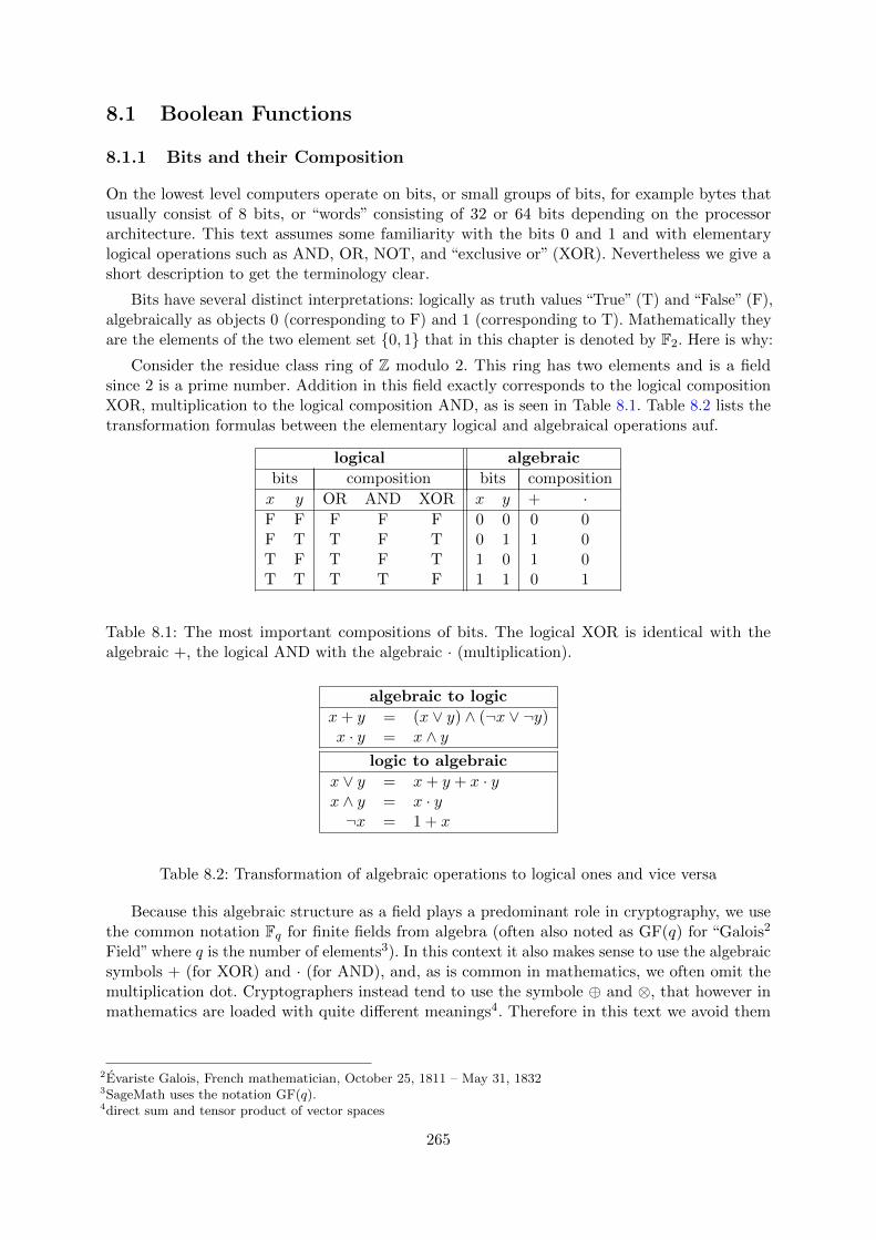
8.1 Boolean Functions
8.1.1 Bits and their Composition
On the lowest level computers operate on bits, or small groups of bits, for example bytes thatusually consist of 8 bits, or “words” consisting of 32 or 64 bits depending on the processorarchitecture. This text assumes some familiarity with the bits 0 and 1 and with elementarylogical operations such as AND, OR, NOT, and “exclusive or” (XOR). Nevertheless we give ashort description to get the terminology clear.
Bits have several distinct interpretations: logically as truth values “True” (T) and “False” (F),algebraically as objects 0 (corresponding to F) and 1 (corresponding to T). Mathematically theyare the elements of the two element set {0, 1} that in this chapter is denoted by F2. Here is why:
Consider the residue class ring of Z modulo 2. This ring has two elements and is a fieldsince 2 is a prime number. Addition in this field exactly corresponds to the logical compositionXOR, multiplication to the logical composition AND, as is seen in Table 8.1. Table 8.2 lists thetransformation formulas between the elementary logical and algebraical operations auf.
logical algebraic
bits composition bits composition
x y OR AND XOR x y + ·F F F F F 0 0 0 0F T T F T 0 1 1 0T F T F T 1 0 1 0T T T T F 1 1 0 1
Table 8.1: The most important compositions of bits. The logical XOR is identical with thealgebraic +, the logical AND with the algebraic · (multiplication).
algebraic to logic
x+ y = (x ∨ y) ∧ (¬x ∨ ¬y)x · y = x ∧ y
logic to algebraic
x ∨ y = x+ y + x · yx ∧ y = x · y¬x = 1 + x
Table 8.2: Transformation of algebraic operations to logical ones and vice versa
Because this algebraic structure as a field plays a predominant role in cryptography, we usethe common notation Fq for finite fields from algebra (often also noted as GF(q) for “Galois2
Field” where q is the number of elements3). In this context it also makes sense to use the algebraicsymbols + (for XOR) and · (for AND), and, as is common in mathematics, we often omit themultiplication dot. Cryptographers instead tend to use the symbole ⊕ and ⊗, that however inmathematics are loaded with quite different meanings4. Therefore in this text we avoid them
2Evariste Galois, French mathematician, October 25, 1811 – May 31, 18323SageMath uses the notation GF(q).4direct sum and tensor product of vector spaces
265
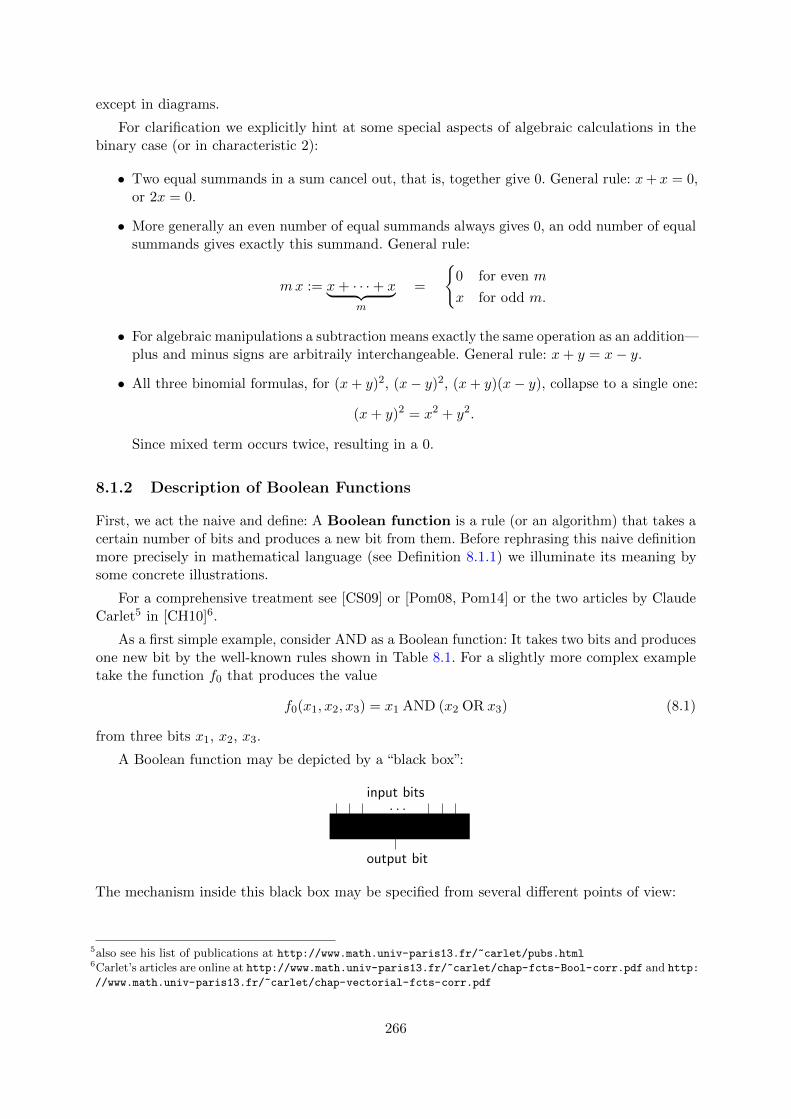
except in diagrams.
For clarification we explicitly hint at some special aspects of algebraic calculations in thebinary case (or in characteristic 2):
• Two equal summands in a sum cancel out, that is, together give 0. General rule: x+ x = 0,or 2x = 0.
• More generally an even number of equal summands always gives 0, an odd number of equalsummands gives exactly this summand. General rule:
mx := x+ · · ·+ x︸ ︷︷ ︸m
=
{0 for even m
x for odd m.
• For algebraic manipulations a subtraction means exactly the same operation as an addition—plus and minus signs are arbitraily interchangeable. General rule: x+ y = x− y.
• All three binomial formulas, for (x+ y)2, (x− y)2, (x+ y)(x− y), collapse to a single one:
(x+ y)2 = x2 + y2.
Since mixed term occurs twice, resulting in a 0.
8.1.2 Description of Boolean Functions
First, we act the naive and define: A Boolean function is a rule (or an algorithm) that takes acertain number of bits and produces a new bit from them. Before rephrasing this naive definitionmore precisely in mathematical language (see Definition 8.1.1) we illuminate its meaning bysome concrete illustrations.
For a comprehensive treatment see [CS09] or [Pom08, Pom14] or the two articles by ClaudeCarlet5 in [CH10]6.
As a first simple example, consider AND as a Boolean function: It takes two bits and producesone new bit by the well-known rules shown in Table 8.1. For a slightly more complex exampletake the function f0 that produces the value
f0(x1, x2, x3) = x1 AND (x2 OR x3) (8.1)
from three bits x1, x2, x3.
A Boolean function may be depicted by a “black box”:
XgXXXXXXXXXX
. . .input bits
output bit
The mechanism inside this black box may be specified from several different points of view:
5also see his list of publications at http://www.math.univ-paris13.fr/~carlet/pubs.html6Carlet’s articles are online at http://www.math.univ-paris13.fr/~carlet/chap-fcts-Bool-corr.pdf and http:
//www.math.univ-paris13.fr/~carlet/chap-vectorial-fcts-corr.pdf
266
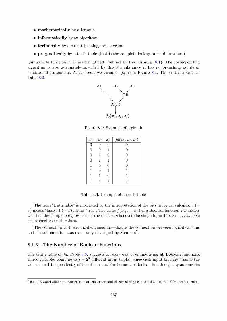
• mathematically by a formula
• informatically by an algorithm
• technically by a circuit (or plugging diagram)
• pragmatically by a truth table (that is the complete lookup table of its values)
Our sample function f0 is mathematically defined by the Formula (8.1). The correspondingalgorithm is also adequately specified by this formula since it has no branching points orconditional statements. As a circuit we visualize f0 as in Figure 8.1. The truth table is inTable 8.3.
AND
?f0(x1, x2, x3)
x1 x2 x3
OR
�
�@R@@@@R
Figure 8.1: Example of a circuit
x1 x2 x3 f0(x1, x2, x3)
0 0 0 00 0 1 00 1 0 00 1 1 01 0 0 01 0 1 11 1 0 11 1 1 1
Table 8.3: Example of a truth table
The term “truth table” is motivated by the interpretation of the bits in logical calculus: 0 (=F) means “false”, 1 (= T) means “true”. The value f(x1, . . . , xn) of a Boolean function f indicateswhether the complete expression is true or false whenever the single input bits x1, . . . , xn havethe respective truth values.
The connection with electrical engineering—that is the connection between logical calculusand electric circuits—was essentially developed by Shannon7.
8.1.3 The Number of Boolean Functions
The truth table of f0, Table 8.3, suggests an easy way of enumerating all Boolean functions:Three variables combine to 8 = 23 different input triples, since each input bit may assume thevalues 0 or 1 independently of the other ones. Furthermore a Boolean function f may assume the
7Claude Elwood Shannon, American mathematician and electrical engineer, April 30, 1916 – February 24, 2001.
267
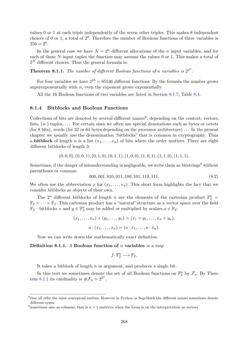
values 0 or 1 at each triple independently of the seven other triples. This makes 8 independentchoices of 0 or 1, a total of 28. Therefore the number of Boolean functions of three variables is256 = 28.
In the general case we have N = 2n different allocations of the n input variables, and foreach of these N input tuples the function may assume the values 0 or 1. This makes a total of2N different choices. Thus the general formula is:
Theorem 8.1.1. The number of different Boolean functions of n variables is 22n
.
For four variables we have 216 = 65536 different functions. By the formula the number growssuperexponentially with n, even the exponent grows exponentially.
All the 16 Boolean functions of two variables are listed in Section 8.1.7, Table 8.4.
8.1.4 Bitblocks and Boolean Functions
Collections of bits are denoted by several different names8, depending on the context: vectors,lists, (n-) tuples, . . . For certain sizes we often use special denotations such as bytes or octets(for 8 bits), words (for 32 or 64 bytes depending on the processor architecture) . . . In the presentchapter we usually use the denomination “bitblocks” that is common in cryptography. Thusa bitblock of length n is a list (x1, . . . , xn) of bits where the order matters. There are eightdifferent bitblocks of length 3:
(0, 0, 0), (0, 0, 1), (0, 1, 0), (0, 1, 1), (1, 0, 0), (1, 0, 1), (1, 1, 0), (1, 1, 1).
Sometimes, if the danger of misunderstanding is negligeable, we write them as bitstrings9 withoutparentheses or commas:
000, 001, 010, 011, 100, 101, 110, 111. (8.2)
We often use the abbreviation x for (x1, . . . , xn). This short form highlights the fact that weconsider bitblocks as objects of their own.
The 2n different bitblocks of length n are the elements of the cartesian product Fn2 =F2 × · · · × F2. This cartesian product has a “natural” structure as a vector space over the fieldF2—bitblocks x and y ∈ Fn2 may be added or multiplied by scalars a ∈ F2:
(x1, . . . , xn) + (y1, . . . , yn) = (x1 + y1, . . . , xn + yn),
a · (x1, . . . , xn) = (a · x1, . . . , a · xn).
Now we can write down the mathematically exact definition:
Definition 8.1.1. A Boolean function of n variables is a map
f: Fn2 −→ F2.
It takes a bitblock of length n as argument, and produces a single bit.
In this text we sometimes denote the set of all Boolean functions on Fn2 by Fn. By Theo-rem 8.1.1 its cardinality is #Fn = 22
n.
8that all refer the same conceptual entities. However in Python or SageMath the different names sometimes denotedifferent types.
9sometimes also as columns, that is n× 1 matrices when the focus is on the interpretation as vectors
268

Convention If we describe a Boolean function by its truth table, we usually order the truthtable lexicographically10 with respect to x ∈ Fn2 , as in the example above. This ordercorresponds to the natural order of the integers a = 0, . . . , 2n − 1, if these are expanded inbase 2
a = x1 · 2n−1 + · · ·+ xn−1 · 2 + xn
and assigned to the corresponding bitblocks (x1, . . . , xn) ∈ Fn2 .
8.1.5 Logical Expressions and Conjunctive Normal Form
For describing Boolean functions in mathematical terms, that is by formulas, there are twoapproaches (beyond truth tables):
• In the logical approach Boolean functions are expressed by disjunctions (the operation OR,also written as ∨), conjunctions (the operation AND, also written as ∧), and negations (theoperation NOT, also written as ¬). Compositions of these operations are called logicalexpressions.
• In the algebraic approach Boolean functions are expressed by additions + and multiplica-tions · in the field F2. Compositions of these operations are called (binary) polynomialexpressions11.
We’ll see soon that both approaches describe all Boolean functions, and that we even can require acertain structure as so called normal forms. Of course there are algorithms to switch between thethree representations—truth tables, logical expressions, and binary polynomial expressions—forall Boolean functions. But we cannot hope that these algorithms are efficient for large numbersn of variables—even writing down the truth table involves 2n bits. For the algorithmic treatmentof Boolean functions in SageMath see also Appendix 8.4.
It seems that the algebraic approach allows a smoother handling of Boolean functions forcryptologic purposes due to its (yet to explore) more rigid structure. In contrast the logicalapproach more easily leads to a realization in hardware by circuits since the elementary Booleanoperations have direct analogues as circuit elements (“gates”).
Since in the following the logical approach plays a minor role we state the result on normalforms without further reasoning. The possibility of a logical representation (without normalization)will follow as a corollary in Section 8.1.7, see Theorem 8.1.5.
Theorem 8.1.2. Each Boolean function of n variables x1, . . . , xn has a representation of theform (conjunction)
f(x) = s1(x) ∧ . . . ∧ sr(x)
with some index r where the sj(x) for j = 1, . . . , r each have the form (disjunctions)
sj(x) = tj1(x) ∨ . . . ∨ tjnj (x)
10The lexicographic order orders strings (like a dictionary) by the value of their first characters—here 0 or 1 with0 < 1. If the first characters are equal, the order looks at the second character an so on. The sequence 011, 100, 101is in lexicographic order. A counterexample is the sequence 100, 101, 011: here the third string begins with 0 thatis smaller than the first character of the string preceding it. The sequence of the eight bitblocks of length 3 inFormula (8.2) is in lexicographic order.
11An expression that contains other kinds of operations is non-polynomial. For numbers we could think of usinginput variables as exponents. This however makes little sense for the Boolean variables 0 und 1. But see thedefinition of the Fourier transform in Section 8.2.8.
269
with a certain number nj of terms tjk(x) (j = 1, . . . , r and k = 1, . . . , nj), each of which in turnhas the form xi (an input bit) or ¬xi (a negated input bit) for some index i12.
In other words: We can build each Boolean function by first forming a handful of expressions(the sj(x)) as OR of some of the input bits or their negations, and then join these expressionsby AND (“conjunction of disjunctions”). This “normal form” cleanly separates AND- and OR-compositions into two layers—there is no further intermixture. The example function f0 fromSection 8.1.2 was defined by the formula
f0(x1, x2, x3) = x1︸︷︷︸s1(x)
∧ (x2 ∨ x3)︸ ︷︷ ︸s2(x)
that already has the “conjunctive” form from Theorem 8.1.2 with
n1 = 1, s1(x) = t11(x) = x1, n2 = 2, t21(x) = x2, t22(x) = x3.
This is no longer true if we expand it:
f0(x) = (x1 ∧ x2) ∨ (x1 ∧ x3)
This example doesn’t display negated input bits. However in Table 8.4 we see some of them.
The form of a Boolean function according to Theorem 8.1.2 is called conjunctive normalform (CNF). It is not unique13,14. Without further explanation we remark that there is afurther simplification as a “canonical CNF” that guarantees a certain uniqueness. There is alsoan analoguous disjunctive normal form (DNF) (a “disjunction of conjunctions”).
8.1.6 Polynomial Expressions and Algebraic Normal Form
We consider (binary) polynomial expressions in the variables x1, . . . , xn, such as x21x2 +x2x3 +x23.Since we work over the field F2 only the constants 0 and 1 occur as coefficients and these don’tshow up explicitly. The observation15 that a2 = a for all elements a ∈ F2, and even ae = a forall exponents e ≥ 1, leads to another simplification of the expressions. As a consequence forbinary polynomial expressions we need consider the variables x1, . . . , xn with exponents 0 and 1only. Therefore our sample expression may be written as x1x2 + x2x3 + x3. Another example:x31x2 + x1x
22 = x1x2 + x1x2 = 0.
In general a monomial expression (or simply “monomial”) has the form
xI :=∏i∈I
xi with a subset I ⊆ {1, . . . , n},
in other words it is a product of some of the variables where the subset I specifies the choice of“some”. Here is an illustrative example with n = 3:
I = {2, 3} =⇒ xI = x2x3
12In particular nj ≤ n for j = 1, . . . , r. Each individual input bit xi occurs in each of the tjk(x) either directly, ornegated or not at all.
13For example we could add the terms ∧ (x1 ∨ x2) ∧ (x1 ∨ x3) to the normal form of f0.14The SageMath class sage.logic.boolformula.BooleanFormula provides transformations of a logical expression
to the CNF by the function convert_cnf(), and to the corresponding truth table by the function truthtable().15Note 02 = 0 and 12 = 1.
270

The total number of such monomial expressions is exactly 2n, corresponding to the number ofchoices of products of n potential factors. Here the empty set corresponds to an “empty” productof 0 factors whose usual interpretation is 116. Thus
I = ∅ =⇒ xI = 1
A monomial expression has an immediate interpretation as a Boolean function. At first sight wedon’t know whether all of these functions are distinct, but we’ll see this in a few moments.
A polynomial expression is a sum of monomial expressions—remember that we are inthe binary case where coefficients take the values 0 or 1 only. Thus the most general (binary)polynomial expression has the form ∑
I⊆{1,...,n}
aIxI ,
where all coefficients aI are 0 or 1. In other words we add a subset of the 2n potential monomialexpressions, and for this we have 22
nchoices. All these expressions give different Boolean
functions, but we yet have to prove this. At first we prove that each Boolean function has apolynomial expression.
Theorem 8.1.3 (ANF). For each Boolean function f: Fn2 −→ F2 there are coefficients aI ∈ F2
(that is = 0 or 1), where I runs through all subsets of {1, . . . , n}, such that f may be written asa polynomial expression in n variables of the form:
f(x1, . . . , xn) =∑
I⊆{1,...,n}
aIxI . (8.3)
Proof(Induction on n) Start with n = 117. The four Boolean functions of one variable x are theconstants 0 and 1 and the functions given by x and 1 + x (= the negation of x). They all havethe claimed form.
Now let n ≥ 1. For x = (x1, . . . , xn) ∈ Fn2 we abbreviate (x2, . . . , xn) ∈ Fn−12 as x′. Then wecan also write x = (x1, x
′) instead of x = (x1, . . . , xn).
Now take a function f ∈ Fn. For each fixed value b of the first variable x1, the choices beingb = 0 or b = 1, we consider the function x′ 7→ f(b, x′) of the n− 1 variables that x′ consists of.By induction (for b = 0 as well as for b = 1) we know
f(b, x′) = pb(x′) for all x′ ∈ Fn−12
where p0, p1 are polynomial expressions in x′ of the desired form:
p0(x′) =
∑J⊆{2,...,n}
bJxJ , p1(x
′) =∑
J⊆{2,...,n}
cJxJ .
Therefore
f(x1, x′) =
{p0(x
′), if x1 = 0,
p1(x′), if x1 = 1,
for all x = (x1, x′) ∈ Fn2
since x1 assumes the values 0 or 1 only. We combine this conditional formula into
f(x1, x′) = (1 + x1) p0(x
′) + x1 p1(x′) for all x ∈ Fn2 (8.4)
16whereas “empty” sums usually are interpreted as 0.17As a “typical mathematical sophistry” we could start with n = 0—the constant polynomial expressions 0 and 1
correspond to the two possible constant functions of 0 variables.
271

(To check this formula substitute x1 = 0 or x1 = 1). By expanding the right hand side andeliminating repeated monomials we get a polynomial expression in x of the claimed form:
f(x1, x′) = p0(x
′) + x1(p0(x′) + p1(x
′))
=∑
J⊆{2,...,n}
bJxJ
︸ ︷︷ ︸all monomials without x1
+∑
J⊆{2,...,n}
(bJ + cJ)x1xJ .
︸ ︷︷ ︸all monomials with x1
2
The wording of this theorem is mathematically compact. As an illustration look at the secondcolumn of table 8.4, where the variables are x and y instead of x1 and x2, and the coefficientsare a, b, c, d instead of a∅, a{1}, a{2}, a{1,2}. Each row of the table describes a Boolean functionof two variables. The corresponding polynomial expression is the sum of the terms 1, x, y, xythat have coefficient 1 in the representation by Equation (8.3), whereas terms with coefficients 0don’t show up explicitly.
Theorem 8.1.3 provides a representation of a Boolean function as a polynomial expression.This expression is called the algebraic normal form (ANF)18. The ANF is unique: Sincethe total number of polynomial expressions is 22
n, and since they represent all 22
ndifferent
Boolean functions, all these polynomial expressions must differ as functions, and furthermorethis representation of a Boolean function as a polynomial expression must be unique. We haveshown:
Theorem 8.1.4. The representation of a Boolean function in algebraic normal form is unique.
Definition 8.1.2. The (algebraic) degree of a Boolean function f ∈ Fn is the degree of itspolynomial expression in algebraic normal form,
deg f = max{#I | aI 6= 0}.
It is always ≤ n.
The degree indicates how many different variables maximally occur in a monomial of theANF.
Example Independently of the number of variables there are exactly two Boolean functions ofdegree 0: the two Boolean constants 0 and 1.
Functions of degree ≤ 1 are called affine functions. They are a sum of a constant and a Booleanlinear form, see Section 8.1.9. If the degree is > 1 the function is called nonlinear, even thoughthe denomination “non-affine” would be more correct.
Example The Boolean function given by x 7→ x1x2 + x2x3 + x3 has degree 2.
Remark Boolean functions have a high degree not by high powers of some variables but “only”by large products of different variables. Each single variable occurs with exponent at most1 in each monomial of the ANF. Another way to express this fact is to say that all partialdegrees—the degrees in the single variables xi without regard for the other variables—are≤ 1.
18The transformation of ANF to truth table and vice versa is provided by the (internal) function __convert()
of the class BoolF(), see SageMath sample 8.42. SageMath’s own module sage.crypto.boolean_function alsoprovides initialization by a truth table or by a Boolean polynomial, and functions algebraic_normal_form() andtruth_table() for the transformations.
272

8.1.7 Boolean Functions of Two Variables
All the 24 = 16 Boolean functions of two variables x and y are enumerated in Table 8.4, aspolynomial expressions in algebraic normal form a+ bx+ cy + dxy, and as logical expressions.The parameters aI from Theorem 8.1.3 translate as follows: a = a∅, b = a{1}, c = a{2}, d = a{1,2},the input variables as x = x1, y = x2.
a b c d ANF logical operation CNF
0 0 0 0 0 False constant x ∧ ¬x1 0 0 0 1 True constant x ∨ ¬x0 1 0 0 x x projection x
1 1 0 0 1 + x ¬x negation ¬x0 0 1 0 y y projection y
1 0 1 0 1 + y ¬y negation ¬y0 1 1 0 x+ y x XOR y XOR (x ∨ y) ∧ (¬x ∨ ¬y)
1 1 1 0 1 + x+ y x⇐⇒ y equivalence (¬x ∨ y) ∧ (x ∨ ¬y)
0 0 0 1 xy x ∧ y AND x ∧ y1 0 0 1 1 + xy ¬(x ∧ y) NAND (¬x) ∨ (¬y)
0 1 0 1 x+ xy x ∧ (¬y) x ∧ (¬y)
1 1 0 1 1 + x+ xy x =⇒ y implication (¬x) ∨ y0 0 1 1 y + xy (¬x) ∧ y (¬x) ∧ y1 0 1 1 1 + y + xy x⇐= y implication x ∨ (¬y)
0 1 1 1 x+ y + xy x ∨ y OR x ∨ y1 1 1 1 1 + x+ y + xy ¬(x ∨ y) NOR (¬x) ∧ (¬y)
Table 8.4: The 16 operations on two bits (= Boolean functions of 2 variables), using Table 8.2(The order of the first column is lexicographic if a, b, c, d are considered in reverse order.)
We have already seen that each Boolean function admits a polynomial expression. To showthat each Boolean function also admits a logical expression we only have to make sure that thealgebraic operations + and · have expressions by the logical operations ∨, ∧, and ¬. To see thislook at the corresponding rows of Table 8.4. Thus we have shown (as a weak form of the hereunproven Theorem 8.1.2):
Theorem 8.1.5. Each Boolean function admits a logical expression, that is a representation bya composition of the logical operations ∨, ∧, and ¬.
Hint In the algebraic interpretation the logical negation ¬ corresponds to the addition of 1.
Remark The analogous form of the ANF for a Boolean function of three variables x, y, z is19
(x, y, z) 7→ a+ bx+ cy + dz + exy + fxz + gyz + hxyz.
Here we see 8 coefficients a, . . . , h. This fits the observations that
19In this formula the letter f—in contrast with the common use in this text—denotes a coefficient, not a function.Mathematicians almost always use letters as symbols relative to the context, and only in exceptional cases withan absolute meaning. Such exceptions are the numbers e, i, and π. But even i often denotes—in contexts withoutcomplex numbers—some other object, for example an index in a sum. Or sometimes e is used as exponent, orcoefficient.
273
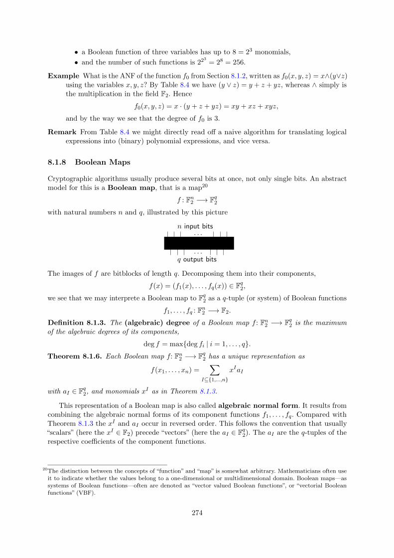
• a Boolean function of three variables has up to 8 = 23 monomials,
• and the number of such functions is 223
= 28 = 256.
Example What is the ANF of the function f0 from Section 8.1.2, written as f0(x, y, z) = x∧(y∨z)using the variables x, y, z? By Table 8.4 we have (y ∨ z) = y + z + yz, whereas ∧ simply isthe multiplication in the field F2. Hence
f0(x, y, z) = x · (y + z + yz) = xy + xz + xyz,
and by the way we see that the degree of f0 is 3.
Remark From Table 8.4 we might directly read off a naive algorithm for translating logicalexpressions into (binary) polynomial expressions, and vice versa.
8.1.8 Boolean Maps
Cryptographic algorithms usually produce several bits at once, not only single bits. An abstractmodel for this is a Boolean map, that is a map20
f : Fn2 −→ Fq2with natural numbers n and q, illustrated by this picture
XgXXXXXXXXXX
. . .
. . .
n input bits
q output bits
The images of f are bitblocks of length q. Decomposing them into their components,
f(x) = (f1(x), . . . , fq(x)) ∈ Fq2,
we see that we may interprete a Boolean map to Fq2 as a q-tuple (or system) of Boolean functions
f1, . . . , fq : Fn2 −→ F2.
Definition 8.1.3. The (algebraic) degree of a Boolean map f: Fn2 −→ Fq2 is the maximumof the algebraic degrees of its components,
deg f = max{deg fi | i = 1, . . . , q}.Theorem 8.1.6. Each Boolean map f: Fn2 −→ Fq2 has a unique representation as
f(x1, . . . , xn) =∑
I⊆{1,...,n}
xIaI
with aI ∈ Fq2, and monomials xI as in Theorem 8.1.3.
This representation of a Boolean map is also called algebraic normal form. It results fromcombining the algebraic normal forms of its component functions f1, . . . , fq. Compared withTheorem 8.1.3 the xI and aI occur in reversed order. This follows the convention that usually“scalars” (here the xI ∈ F2) precede “vectors” (here the aI ∈ Fq2). The aI are the q-tuples of therespective coefficients of the component functions.
20The distinction between the concepts of “function” and “map” is somewhat arbitrary. Mathematicians often useit to indicate whether the values belong to a one-dimensional or multidimensional domain. Boolean maps—assystems of Boolean functions—often are denoted as “vector valued Boolean functions”, or “vectorial Booleanfunctions” (VBF).
274
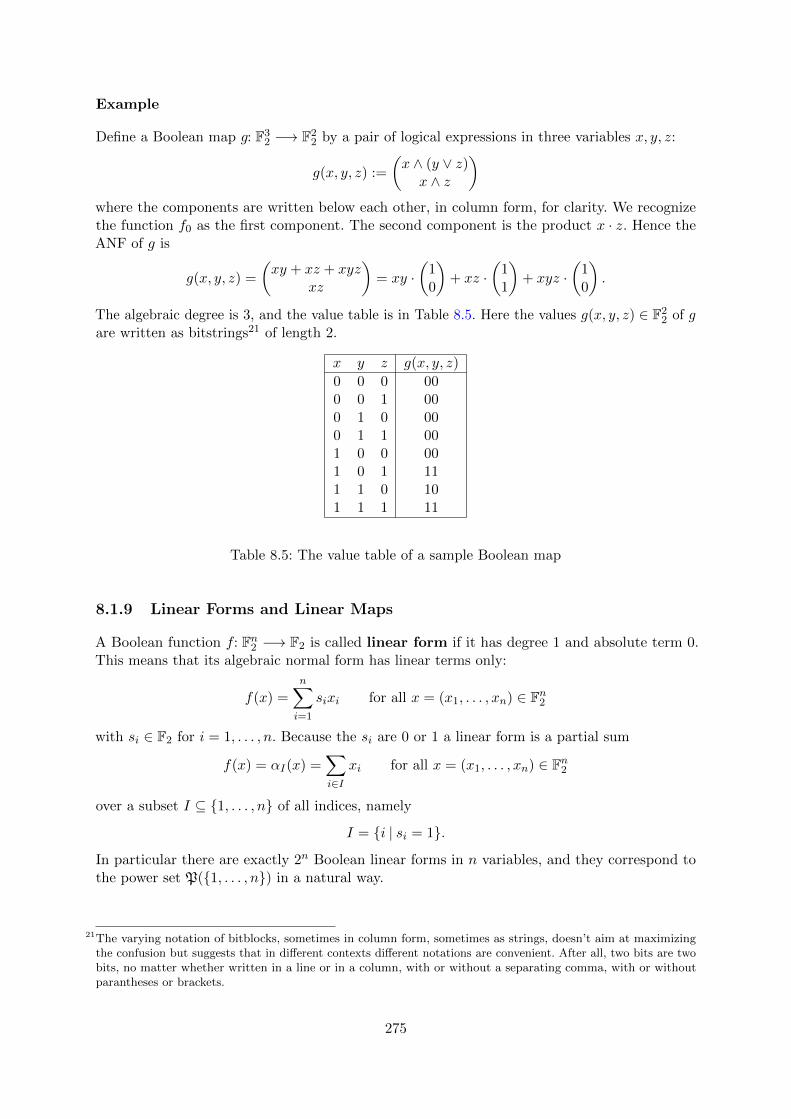
Example
Define a Boolean map g: F32 −→ F2
2 by a pair of logical expressions in three variables x, y, z:
g(x, y, z) :=
(x ∧ (y ∨ z)x ∧ z
)where the components are written below each other, in column form, for clarity. We recognizethe function f0 as the first component. The second component is the product x · z. Hence theANF of g is
g(x, y, z) =
(xy + xz + xyz
xz
)= xy ·
(10
)+ xz ·
(11
)+ xyz ·
(10
).
The algebraic degree is 3, and the value table is in Table 8.5. Here the values g(x, y, z) ∈ F22 of g
are written as bitstrings21 of length 2.
x y z g(x, y, z)
0 0 0 000 0 1 000 1 0 000 1 1 001 0 0 001 0 1 111 1 0 101 1 1 11
Table 8.5: The value table of a sample Boolean map
8.1.9 Linear Forms and Linear Maps
A Boolean function f: Fn2 −→ F2 is called linear form if it has degree 1 and absolute term 0.This means that its algebraic normal form has linear terms only:
f(x) =n∑i=1
sixi for all x = (x1, . . . , xn) ∈ Fn2
with si ∈ F2 for i = 1, . . . , n. Because the si are 0 or 1 a linear form is a partial sum
f(x) = αI(x) =∑i∈I
xi for all x = (x1, . . . , xn) ∈ Fn2
over a subset I ⊆ {1, . . . , n} of all indices, namely
I = {i | si = 1}.
In particular there are exactly 2n Boolean linear forms in n variables, and they correspond tothe power set P({1, . . . , n}) in a natural way.
21The varying notation of bitblocks, sometimes in column form, sometimes as strings, doesn’t aim at maximizingthe confusion but suggests that in different contexts different notations are convenient. After all, two bits are twobits, no matter whether written in a line or in a column, with or without a separating comma, with or withoutparantheses or brackets.
275

Other common notations are (for I = {i1, . . . , ir}):
f(x) = αI(x) = x[I] = x[i1, . . . , ir] = xi1 + · · ·+ xir .
The following theorem relates the definition with the notion of linear forms from linearalgebra:
Theorem 8.1.7. A Boolean function f: Fn2 −→ F2 is a linear form if and only if the followingtwo conditions hold:
(i) f(x+ y) = f(x) + f(y) for all x, y ∈ Fn2 .
(ii) f(ax) = af(x) for all a ∈ F2 and all x ∈ Fn2 .
ProofThe representation by partial sums shows that each linear form meets the two conditions.
For the reverse direction let f be a Boolean function with (i) and (ii). Let e1 = (1, 0, . . . , 0),. . . , en = (0, . . . , 1) be the “canonical unit vectors”. Then each x = (x1, . . . , xn) ∈ Fn2 is a sum
x = x1e1 + · · ·+ xnen.
Hencef(x) = f(x1e1) + · · ·+ f(xnen) = x1f(e1) + · · ·+ xnf(en)
is the partial sum of the xi over the index set consisting of the i for which the constant valuef(ei) is 1. Therefore f is a linear form in the sense of the definition above. 2
A Boolean map f: Fn2 −→ Fq2 is called linear if all of its component functions f1, . . . , fq arelinear forms. As in the case q = 1 we can show:
Theorem 8.1.8. A Boolean map f: Fn2 −→ Fq2 is linear if and only if the following two conditionshold:
(i) f(x+ y) = f(x) + f(y) for all x, y ∈ Fn2 .
(ii) f(ax) = af(x) for all a ∈ F2 and all x ∈ Fn2 .
Theorem 8.1.9. A Boolean map f: Fn2 −→ Fq2 is linear if and only if it has the form
f(x) =n∑i=1
xisi
with si ∈ Fq2.
(Here again the xi and si are written in reverse order.)
Affine (Boolean) maps are maps of algebraic degree ≤ 1. They result from adding linearmaps and constants.
In the case q = 1, that is for functions, the only possible constants are 0 and 1. Adding theconstant 1 effects a logical negation, that is a “flipping” of all bits. Therefore we can say: Theaffine Boolean functions are the linear forms and their negations.
276

8.1.10 Systems of Boolean Linear Equations
Linear algebra over the field F2 is quite simple, many complications known from other math-ematical areas boil down to trivialities. Such is the case for the solution of systems of linearequations, explicitly written as
a11x1 + · · · + a1nxn = b1...
......
am1x1 + · · · + amnxn = bm
with given aij and bi ∈ F2, and unknown xj for which we search solutions. In matrix terms thissystem has an elegant expression as
Ax = b
where A is an m× n matrix, and x and b are column vectors, that is n× 1 or m× 1 matrices.
Systems of Linear Equations in SageMath
To clarify the relation with “common” linear algebra we consider an example of a system of linearequations over the rational numbers:
x1 + 2x2 + 3x3 = 03x1 + 2x2 + x3 = −4x1 + x2 + x3 = −1
and study how to handle this in SageMath. The complete solution is in SageMath sample 8.1.Here are the single steps:
1. Define the “coefficient matrix”A =
1 2 33 2 11 1 1
.
2. Define the “image vevtor” b = (0,−4, 1).
3. Let SageMath calculate a “solution vector” x. Since we wrote the left hand side of thesystem as matrix product Ax we have to use the method solve_right().
4. Our system of linear equations could admit several solutions. We find them all by solvingthe corresponding “homogeneous”22 system Az = 0. If z is a solution of the homogeneoussystem, then A · (x + z) = Ax + Az = b + 0 = b, so x + z is a solution of the original(“inhomogeneneous”) system. In this way we get all solutions. For if Ax = b and Ay = b,then A · (y − x) = 0, hence the difference y − x solves the homogeneous system. For thesolution of the homogeneous system we use the SageMath method right_kernel().
5. The output appears somewhat cryptic. It says23 that all solutions of the homogeneoussystem are multiples of the vector z = (1,−2, 1).
6. We verify the solution y = x− 4z by checking that Ay = b.
22replacing the right hand side b by 023Since all coefficients were integers SageMath worked over Z (= Integer Ring).
277

SageMath sample 8.1 Solution of a system of linear equations over Q
sage: A = Matrix([[1,2,3],[3,2,1],[1,1,1]])
sage: b = vector([0,-4,-1])
sage: x = A.solve_right(b); x
(-2, 1, 0)
sage: K = A.right_kernel(); K
Free module of degree 3 and rank 1 over Integer Ring
Echelon basis matrix:
[ 1 -2 1]
sage: y = x - 4*vector([1,-2,1]); y
(-6, 9, -4)
sage: A*y
(0, -4, -1)
Systems of Linear Equations in the Boolean Case
In the general case (over an arbitrary field) the underlying algorithm for solving a system oflinear equations is Gaussian24 elimination. This algorithm of course also hides in the SageMathmethod solve_right().
In the Boolean case (over the field F2) the solution of a system of linear equations by Gaussianelimination is extremely simple since all coefficients are 0 or 1, and multiplication and divisionare completely trivial. We don’t need to deal with complicated coefficients (such as fractionsover Q), or inexact coefficients (such as floating point numbers over R). So simple is the methodthat even for six unknowns calculating by “paper and pencil” almost outperforms the feedingof the corresponding small SageMath program with the correct input values. An example willillustrate this effect.
The idea of elimination is: reduce the system to a system with only n − 1 unknowns, or“eliminate” one unknown.
Case 1 xn only occurs with coefficients ain = 0 for i = 1, . . . ,m. In other words, xn doesn’toccur at all. Then the system is already reduced.
Case 2 xn has coefficient 1 in one of the equations. Then solve this25 equation for xn, andsubstitute the resulting expression for xn,
xn = ai1x1 + · · · ai,n−1xn−1 + bi,
in the other m− 1 equations. Thereafter the remaining equations contain only the unknownsx1, . . . , xn−1.
Continue recursively until there remains only one unknown or one equation. Now for the examplethat illustrates this simple procedure.
24Johann Carl Friedrich Gauß, German mathematician, astronomer, geodesist, and physicist, April 30, 1777 –February 23, 1855
25If we have more than one choice it doesn’t matter which one we choose—in contrast to the situation over otherfields where the search for an optimal “pivot element” constitutes an essential part of the algorithm.
278

Example
x1 +x3 +x6 = 1x1 +x2 +x4 +x6 = 0
x2 +x3 +x5 +x6 = 0x1 +x4 +x5 = 1
x2 +x4 +x5 = 1
From the first equation we get x6 = x1 +x3 +1 (using the rule that plus and minus are the same).Elimination results in a reduced system consisting of the equations 2 to 5 (note x1 + x1 = 0 etc.):
x2 +x3 +x4 = 1x1 +x2 +x5 = 1x1 +x4 +x5 = 1
x2 +x4 +x5 = 1
Solving the second equation of the reduced system for x5 and substituting x5 = x1 + x2 + 1 inthe other ones gives
x2 +x3 +x4 = 1x2 +x4 = 0
x1 +x4 = 0
Now the last two equations yield x4 = x2 = x1, and then the first one yields x3 = 1. Thus thecomplete solution is
x1 = x2 = x4 = x6 = a with a ∈ F2 arbitrary, x3 = 1, x5 = 1.
Since a may assume the values 0 and 1 our result consists of exactly two solutions: (0, 0, 1, 0, 1, 0)and (1, 1, 1, 1, 1, 1).
The Example in SageMath
SageMath sample 8.2 shows the solution in SageMath code. The SageMath methodsolve_right() gives the solution (0, 0, 1, 0, 1, 0) only. To get all solutions we have to solvethe homogeneous system. Its solutions are the multiples of the vector v = (1, 1, 0, 1, 0, 1), that is,the two vectors (0, 0, 0, 0, 0, 0) = 0 · v and (1, 1, 0, 1, 0, 1) = 1 · v. Thus the second solution of theinhomogeneous system is (0, 0, 1, 0, 1, 0) + (1, 1, 0, 1, 0, 1) = (1, 1, 1, 1, 1, 1).
Estimate of the Cost
What about the cost of solving a system of Boolean linear equations in general? Consider mequations with n unknowns. Then the matrix A of coefficients has size m× n. The expandedmatrix (A, b) has size m× (n+ 1).
We only aim at a coarse estimate and neglect possible optimizations of the procedure. Forsimplicity we assume m = n. In the case m > n we would ignore additional equations26. In thecase m < n we would append “null equations” (of the kind 0 · x1 + · · ·+ 0 · xn = 0).
The elimination step, that is the reduction of the problem size from n to n− 1, amounts toexactly one pass through all n rows of the expanded matrix:
26Of course we must check if the solutions we found also satisfy the additional equations.
279

SageMath sample 8.2 Solution of a system of Boolean linear equations
sage: M = MatrixSpace(GF(2), 5, 6) # GF(2) = field with two elements
sage: A = M([[1,0,1,0,0,1],[1,1,0,1,0,1],[0,1,1,0,1,1],[1,0,0,1,1,0],\
[0,1,0,1,1,0]]); A
[1 0 1 0 0 1]
[1 1 0 1 0 1]
[0 1 1 0 1 1]
[1 0 0 1 1 0]
[0 1 0 1 1 0]
sage: b = vector(GF(2),[1,0,0,1,1])
sage: x = A.solve_right(b); x
(0, 0, 1, 0, 1, 0)
sage: K = A.right_kernel(); K
Vector space of degree 6 and dimension 1 over Finite Field of size 2
Basis matrix:
[1 1 0 1 0 1]
• At first we search the first entry 1 in column n, consisting of the coefficients of xn. Thiscosts at most n single bit comparisions.
• Then we add the chosen row (containing the first entry 1 in column n) to all thoserows below it that also contain a 1 in column n. This amounts (per row) to a single bitcomparision and up to n bit additions—we ignore the n-th entry since we know alreadythat it becomes 0.
All in all this makes n bit comparisions and at most n · (n− 1) bit additions, a total of at mostn2 bit operations. Let N(n) be the number of bit operations for the complete solution of thesystem. Then we have the following inequality:
N(n) ≤ n2 +N(n− 1) for all n ≥ 2.
Now N(1) = 1: We only have to check the one coefficient of the one unknown whether it is 0 or1. From this we decide whether the equation has a unique solution (for coefficient 1), or whetherit is never true (coefficient 0, right hand side b = 1), or whether it is true for arbitrary values ofthe unknown (coefficient 0, right hand side b = 0).
Then we conclude N(2) ≤ 22 + 1, N(3) ≤ 32 + 22 + 1 etc. By induction we immediately get
N(n) ≤n∑i=1
i2.
The explicit value of this sum is well-known, and we have shown:
Theorem 8.1.10. The number N(n) of needed bit comparisions and bit additions for solving asystem of n Boolean linear equations with n unknowns is upper bounded by
N(n) ≤ 1
6· n · (n+ 1) · (2n+ 1).
A somewhat more sloppy wording of this result expresses the cost as O(n3). In any case it is“polynomial of small degree” in terms of the problem size n.
280
Remark The notation by “O” obscures the difference with the cost over arbitrary fields thatis generally bounded by O(n3). The “felt” much better performance in the Boolean caseis partly founded by the exact estimate in Theorem 8.1.10 that even in the worst case isabout 1
3 · n3. Moreover in the Boolean case we count simple bit operations only, and not
arithmetic operations or floating point instructions that are significantly more expensive.
8.1.11 The Representation of Boolean Functions and Maps
Various Interpretations of Bitblocks
We used the term bitblock for a variety of slightly different objects. A bitblock b = (b1, . . . , bn) ∈Fn2 describes:
• a vector b ∈ Fn2 written as a row or a column. This is the primary meaning of the termbitblock27.
• an argument of a Boolean function or map of n variables, also used as row index of a valuetable (or truth table)
• a bitstring of length n
• a subset I ⊆ {1, . . . , n} defined by b as indicator: i ∈ I ⇔ bi = 1
• a linear form α on Fn2 expressed as sum of the variables xi with bi = 1. The evaluation ofα comes down to the scalar product of vectors: α(x) = b · x.
• a monomial in n variables x1, . . . , xn with all partial degrees ≤ 1. In this interpretation bispecifies the exponent 0 or 1 of the variable xi.
• an integer between 0 and 2n − 1 in binary representation (that is in the base-2 system).The sequence of binary “digits” (= bits) is identical with the corresponding bitstring28.Conversely the integer is the index (beginning with 0) of the bitstring when the biststringsare lexicographically ordered in a list.
Of course there are further interpretations—after all each piece of information has a binary coding.The bitblocks for n = 3 are listed in Table 8.6. SageMath sample 8.4.3 has some transformationfunctions.
Representation of the Truth Table of a Boolean Function
The previous subsection described (and Table 8.6 illustrated) how to interpret the bitblocksx = (x1, . . . , xn) of length n as integers i(x) = 0, 1, . . . , 2n − 1 in base-2 representation. Theexample in Table 8.7 suggests how to describe the truth table of a Boolean function f: Fn2 −→ F2
in a parsimonious way by a bitblock b = (b0, . . . , b2n−1) of length 2n: simply take the last columnin the order given by the indices i(x). The general procedure for arbitrary n runs as follows:
bi(x) = f(x) where i(x) = x1 · 2n−1 + · · ·+ xn−1 · 2 + xn
for x = (x1, . . . , xn) ∈ Fn2 .
27in Python/SageMath implemented as list, or tuple, or vector28The SageMath method binary() transforms an integer to a bitstring, suppressing leading zeros. Example:10.binary() yields ’1010’.
281

integer bitstring subset linear form monomial
0 000 ∅ 0 11 001 {3} x3 x32 010 {2} x2 x23 011 {2, 3} x2 + x3 x2x34 100 {1} x1 x15 101 {1, 3} x1 + x3 x1x36 110 {1, 2} x1 + x2 x1x27 111 {1, 2, 3} x1 + x2 + x3 x1x2x3
Table 8.6: Interpretations of bitblocks of length 3
This might look entangled, but it simply means: “Interpret x as the base-2 representation ofan integer i(x), and set f(x) as the bit at position i(x) from the bitblock b”. An additionalcolumn i(x) in the truth table of the function f0 (f0 was defined in Formula 8.1) illustrates thisprocedure – see Table 8.7. The last column of this table, written in row form, is the bitblock b.
In this way, the bitblock (0, 0, 0, 0, 0, 1, 1, 1) or, even more parsimoniously, the bitstring
00000111
of length 23 = 8 completely specifies the truth table of f0.29
x1 x2 x3 i(x) f0(x1, x2, x3)
0 0 0 0 00 0 1 1 00 1 0 2 00 1 1 3 01 0 0 4 01 0 1 5 11 1 0 6 11 1 1 7 1
Table 8.7: An extended truth table [for f0(x1, x2, x3) = x1 ∧ (x2 ∨ x3)] with n = 3 and 2n = 8
Representation of the Algebraic Normal Form
The algebraic normal form (ANF) also has a characterization by 2n bits: the coefficients of the 2n
different monomials30 (see Theorem 8.1.3, page 271). The monomials also have an interpretationas bitblocks, see the list above. Therefore we may view a bitblock a = (a0, . . . , a2n−1) asrepresentation of the ANF of a Boolean function f : Fn2 −→ F2 in the following way:
f(x) =2n−1∑i=0
aixe1(i)1 · · ·xen(i)n where i = e1(i) · 2n−1 + · · ·+ en(i)
with e1(i), . . . , en(i) = 0 or 1.
29In Python/SageMath bitblocks are implemented as lists.30Remember that the ANF is a sum of monomials. Each monomial is a product of a subset of {x1, . . . , xn}, and
hence has a representation as an integer between 0 und 2n − 1.
282

This formula means: “Interpret the n-tuple e of exponents of a monomial as the base-2 represen-tation of an integer i. The i-th element of the bitblock a indicates whether this monomial occursin the ANF of f or not.”
For the sample function f0 we saw already (or easily check31) that the ANF is
f0(x) = x1x3 + x1x2 + x1x2x3.
It involves the monomials with exponent triples 101, 110, 111 that correspond to the integers5, 6, 7. Therefore we set the bits at the positions 5, 6, 7 to 1, and the remaining bits to 0, and getthe parsimonious representation of the ANF by a bitstring:
00000111.
Warning This is the same bitstring as for the truth table by pure chance—a special propertyof the function f0! The function f(x1, x2) = x1 has truth table 0011 (it takes the value 1 ifand only if x1 = 1, or if the argument has the form x = (1, any bit)) and ANF 0010 (sinceit contains the single monomial x1).
The SageMath class BoolF() has a method for calculating the ANF, see the followingsubsection and Appendix 8.432. SageMath sample 8.3 demonstrates its application to f0.
SageMath sample 8.3 A Boolean function with truth table and ANF
sage: bits = "00000111"
sage: x = str2bbl(bits); x
[0, 0, 0, 0, 0, 1, 1, 1]
sage: f = BoolF(x)
sage: y = f.getTT(); y
[0, 0, 0, 0, 0, 1, 1, 1]
sage: z = f.getANF(); z
[0, 0, 0, 0, 0, 1, 1, 1]
Remark Evaluating a Boolean function f at all arguments x ∈ Fn2 the naive way costs 2n
evaluations f(x), each with at most 2n summands, each of which needing at most n− 1multiplications. Thus the costs have an order of magnitude of about n · 2n · 2n. If we relatethe costs to the input size N = 2n they are essentially quadratic: N2 · log2(N). A commonmethod, binary recursion, or “divide-and-conquer”, divides a problem into two subproblemsof half the input size, and leads to a significantly more efficient algorithm. Starting fromEquation (8.4) in the end effect we achieve a reduction to almost linear costs 3N · log2N .This algorithm33 is implemented in the class BoolF(), see Section 8.4.6.
Object-Oriented Implementation
For an implementation of Boolean functions in SageMath (or Python) see Appendix 8.4.6 (classBoolF()). SageMath itself has a class sage.crypto.boolean_function that contains many
31Remember: f(1, 1, 1) = 1 + 1 + 1 = 1 since we add mod 2.32This transformation that converts a bitstring of length 2n—the truth table—into another bitstring of length 2n—
the coefficient list of the ANF—is sometimes called Reed-Muller transformation or binary Moebius transformation.
33also denoted as fast binary Moebius transformation, an analogue of the fast Fourier transformation (FFT)
283

of the needed methods, also the conversion of a truth table into ANF. Here we describe anindependent implementation.
In general in an object oriented programming language we may define a class that abstractsthe structure of an object “Boolean function”:
Class BoolF:
Attributes:
• blist: truth table as a list of bits (= bitblock in “natural” order as describedin Section 8.1.4). This list is also used as internal representation of the Booleanfunction.
• dim: the dimension of the definition domain
Methods:
• setTT: Fill the truth table with a given bitblock (“TT” for Truth Table).
• setANF: Input the ANF (as a list) and internally transform it into the truth table.
• setDim: Set the dimension.
• getTT: Output the truth table as a bitblock.
• valueAt: Get the value of the Boolean function at a given argument.
• getDim: Output the dimension.
• getANF: Output the algebraic normal form (ANF) as bitblock (in the “natural”order as specified above).
• deg: Output the algebraic degree.
The first three, the “set methods”, are used only implicitly for the initialization of an object. Tohave an easily readable output we add methods printTT and printANF.
The needed functions for transforming bitlists into integers or bitstrings, and vice versa, arein Appendix 8.4.3.
The implementation of Boolean maps derives from this: Define a class BoolMap as a list ofobjects of the class BoolF with (at least) the analoguous methods. Some of them may also befound in the SageMath module sage.crypto.mq.sbox34.
34Cryptographers often use the term “S-boxes” for Boolean maps in small dimensions.
284

8.2 Bitblock Ciphers
In classical cryptography the weakness of simple monoalphabetic substitutions is remedied intwo different ways: first by polygraphic substitutions that encrypt groups of letters at once,second by polyalphabetic substitutions that change the substitution alphabet depending on theposition in the plaintext.
If we consider bits instead of letters, then monoalphabetic substitutions are cryptographicallyuseless since we have only two choices: either leave all bits unchanged or invert all bits. Thusthe plaintext either remains unchanged, or changes in a trivial way. However the two principlesof hardening monoalphabetic substitutions yield two classes of useful encryption methods forbinary encoded informations:
• Bitblock ciphers split bitstrings into blocks of a fixed length and encrypt one completeblock per step.
• Bitstream ciphers encrypt bit by bit, each one by another substitution (so each single bitis unchanged or flipped by a position-dependent rule).
No mathematically complete proof exists for the security of any bitblock or bitstream cipher.Thus the situation is even worse than for asymmetric ciphers where the proof of security oftenreduces to a well-studied, if not solved, mathematical problem. The best we can do is to considera symmetric cipher as secure if none of the known attacks is significantly faster35 than a completeexhaustion of the key space (also known as “brute force attack”).
8.2.1 General Description
Bitblock ciphers transform blocks of a fixed length36 n to bitblocks of the same length controlledby a key that itself is a bitblock of a certain length l.
An adequate model of a bitblock cipher is a Boolean map
F : Fn2 × Fl2 −→ Fn2often interpreted as a family (Fk)k∈K of Boolean maps
Fk : Fn2 −→ Fn2 for all k ∈ K = Fl2where Fk(a) = F (a, k).
Choosing the Key Length
For the key length l we have an obvious criterion: l must be large enough to prevent an exhaustionof the key space, a “brute force attack”. The key space is the set Fl2, so it contains 2l differentkeys. We assume that the probabilities for all keys are the same, that is 1/2l. In other words weassume that keys are chosen uniformly at random.
With these assumption we have a lower bound of about 80 bits for a secure key lengthaccording to the state of the art [LV00]. Popular ciphers use keys of lengths 128 or more, so havea sufficient security margin. The outdated standard cipher DES used 56 bit keys. The technologyof today breaks it quite quickly.
35In this context a factor of less than 10 would not be deemed as “significantly faster”.36The extension of the cipher to bitstrings of arbitrary lengths is the subject of Section 8.2.4. For the moment we
neglect this aspect.
285

Choosing the Block Length
The block length n should be large enough to prevent analyses of patterns or frequencies. Evenmore it should prevent leaking any information about the plaintext into the ciphertext, forexample the presence of repetitions.
If the attacker observes about 2n/2 ciphertexts corresponding to random plaintexts encryptedwith the same key the probability of a “collision”37 is about 1
2 . Therefore this number 2n/2 shouldexceed the number of available memory cells. And the key should change frequently—long beforethis number of blocks is reached.
From this point of view the frequently used block length 64 is risky. Only frequent key changecould justify it, and only if the plaintext contains few repetitions38. A better cipher, as thecurrent standard AES, uses blocks of 128 bits.
These considerations about key or block lengths are typical for the discussion of security inmodern cryptography: We use large security margins and avoid any weaknesses, how small theymight be, even if there is no known practical attack that uses them. But since we have a broadchoice of good and fast ciphers that provide large security margins there is no need to rely on aweaker cipher, even if this precaution seems paranoid.
8.2.2 Algebraic Cryptanalysis
Attacks with Known Plaintext39
Let a bitblock cipher be given by a Boolean map
F : Fn2 × Fl2 −→ Fn2 .
By Theorem 8.1.6 F is an n-tuple F = (F1, . . . Fn) of polynomial expressions in n+ l variablesall of whose partial degrees are ≤ 1.
A known plaintext block a ∈ Fn2 with corresponding ciphertext block c ∈ Fn2 yields a system
F (a, x) = c
of n polynomial equations for the unknown key x ∈ Fl2.Systems of equations of this type (over arbitrary fields) are subjects of algebraic geometry.
The general theory is quite deep, in particular if we search for concrete solution procedures.However—couldn’t the fact that our polynomials have all their partial degrees ≤ 1 simplify theproblem?
Example 1 Let n = l = 2,
F (a1, a2, x1, x2) = (a1 + a2x1, a2 + a1x2 + x1x2),
a = (0, 1), c = (1, 1) ∈ F22. The equations for the key (x1, x2) ∈ F2
2 are(11
)=
(0 + x1
1 + 0 + x1x2
).
The immediate solution is x1 = 1, x2 = 0.
37by the “birthday paradox”38Using a good “mode of operation” avoids the danger of repetitions, see Section 8.2.4.39An attack with known plaintext assumes that the attacker knows or guesses a small piece of plaintext, and then
tries to deduce the key or some more plaintext that is unknown to her. For the present section we assume that theknown plaintext is a complete bitblock.
286

Example 2, linear maps: If F is a linear map, then the system of equations is accessible by theefficient solution algorithms of linear algebra, see 8.1.10. We have n linear equations for lunknowns. If l < n the attacker needs some additional blocks of known plaintext, or sheexecutes an exhaustion of the remaining n− l key bits. For this method to work F needsto be linear only in x.
Example 3, substitution: Often polynomial equations look complex at first sight but aren’t so.Here is an example (over F2)
x1x2x3 + x1x2 + x1x3 + x2x3 + x2 + x3 = 0.
By the substitutions xi = zi + 1 it is transformed to
z1z2z3 + z1 = 0
(for an easy proof look in the reverse direction). This has the solutions
z1 = 0, z2, z3 arbitrary or z1 = z2 = z3 = 1.
Therefore the complete solution of the original equation is
x1 = 1, x2, x3 arbitrary or x1 = x2 = x3 = 0.
There are two powerful general approaches for solving systems of (polynomial) equationsover F2:
• SAT solvers [GJ79]40,
• elimination using Groebner bases [Bri10]41.
Both methods work well for a small number of unknowns. With a growing number of unknownstheir complexity becomes unmanageable42. Of course we always find a solution by searchingthrough the complete value table. But this naive method is inefficient (exponential in the numberof unknowns, and so hopeless for 80 or more unknowns). But also the costs of SAT solvers andGroebner-basis methods grow exponentially with the number of unknowns. Not even the factthat all partial degrees are ≤ 1 is of vital help.
The Complexity of the Algebraic Attack
The theoretical analysis of the cost for finding a solution leads to one of the central notions ofcomplexity theory, NP-completeness.
40SAT denotes the satisfiability problem of propositional logic. Consider a logical expression in Boolean variablesx1, . . . , xn and ask if there exist values of the variables that make the expression “True”. In other words consider aBoolean function f and ask if it assumes the value 1. A SAT solver is an algorithm that takes a logical expressionin CNF and decides the satisfiability by finding a solution x, or showing there’s no solution. The naive algorithmuses the truth table and exhausts the 2n possible arguments. However there are much faster algorithms, the mostpopular being the DPLL algorithm (after Davis, Putnam, Logemann, and Loveland) and BDD based algorithms(Binary Decision Diagram). The SageMath modules sage.sat.solvers and sage.sat.boolean_polynomials
contain some of these algorithms.41For an introduction to this theory see the textbooks [Bar09, CLO07, vzGG99], or the script [Seg04], or the paper
[Laz83].42In fact SAT was the first problem in history shown to be NP-complete.
287

Theorem 8.2.1 (Garey/Johnson). The problem of finding a solution for a system of polynomialequations over F2 is NP complete.
For a proof see the book by Garey/Johnson [GJ79].43
We won’t explain the notion “NP-complete” but only mention that the (up to now unproven)“P 6= NP conjecture” implies that an NP-complete problem admits no efficient algorithmicsolution, or that there is no solution algorithm whose execution time grows at most polynomiallywith the number of input variables.
A common interpretation of this theorem is: For an appropriately chosen block cipherF : Fn2 × Fl2 −→ Fn2 the attack with known plaintext (against the key k ∈ Fl2) is not efficient.However from a strict mathematical point of view the theorem doesn’t prove anything of practicalrelevance:
1. It relates to an algorithm for arbitrary polynomial equations (over F2). It doesn’t containany assertion for special classes of polynomials, or for a concrete system of equations.
2. It gives a pure proof of (non-) existence, and provides no hint as how to construct a concreteexample of a “difficult” system of equations. Note that we know that some concrete systemsadmit easy solutions.
3. Even if we could find concrete examples concrete examples of “difficult” systems the theoremwould not make any assertion whether only some rare instances (the “worst cases”) aredifficult, or almost all (the “generic cases”)—and this is what the cryptologist wants toknow. Maybe there is an algorithm that solves polynomial systems for almost all tuples ofunknowns in an efficient way, and only fails for a few exceptional tuples.
Despite these critical comments the theorem raises hope that there are “secure” bitblock ciphers,and the designers of bitblock ciphers follow the
Rule of thumb Systems of linear equations for bits admit very efficient solutions. Systems ofnonlinear equations for bits in almost all cases admit no efficient solution.
8.2.3 The Structure of Bitblock Ciphers
In an ideal world we would know how to reliably measure the security of a bitblock cipher
F : Fn2 × Fl2 −→ Fn2
for realistic values of the block length n and the key length l, say of an order of magnitude of128 bits or more.
In fact we know explicit measures of security, for example the linear potential, or thedifferential potential, that quantify the deviation from linearity, or the algebraic immunity, orothers. Unfortunately all of these only give necessary, not sufficient, conditions for security, andmoreover the efficient computability of these measures is limited to small block lengths n, about8 or slightly larger.
Lacking a general efficient approach to security the design of bitblock ciphers usually relieson a structure that, although not obligatory, in practice seems to provide plausible security
43A recent article on the difficulty of systems of polynom equations is [CGH+03].
288

round input (n bits)
???. . . . . .
??? key
kn = mq of l bits�����[⊕ or other composition]
?. . .?
. . . . . .?. . .?
S
?. . .?
. . . . . .
. . . . . .
S
?. . .?
P
???. . . . . .
???round output (n bits)
Figure 8.2: A single round of a bitblock cipher (S is a, maybe varying, S-box, P , a permutation,k, the key)
according to verifiable criteria. Most of the generally approved standard ciphers, such as DESand AES, follow this approach.
This common design scheme starts by constructing Boolean maps of small dimensions andthen extending them to the desired block length in several steps:
1. Define one or more Boolean maps of small dimension q (= block length of the definitiondomain), say q = 4, 6, or 8, that are good for several security criteria. These maps arecalled S-boxes44, and are the elementary building blocks of the cipher.
2. Mix the round input with some of the key bits and then apply m S-boxes in parallel (orapply the one S-box m times in parallel) to get a map with the desired input width n = mq.
3. Then permute the complete resulting bitblock over its total width.
4. These steps together are a “round” of the complete scheme. Asset the weaknesses of theround map, that mainly result from using S-boxes of small dimension. Then reduce theseweaknesses in a reasonably controlled way by iterating the scheme over several rounds ofthe same structure but with a changing choice of key bits.
5. Don’t stop as soon as the security measures give satisfying values but add some surplusrounds to get a wide security margin.
Figure 8.2 outlines the scheme for a single round.
The complete scheme is a special case of a somewhat more general proposal that goes backto Shannon who required two basic features of block ciphers:
Diffusion The bits of the plaintext block “smear” over all parts of the block. This is done byapplying permutations (a. k. a. as transpositions).
Confusion (complex dependencies) The interrelation between plaintext block and key on theone hand, as well as ciphertext block on the other hand should be as complex as possible(in particular as nonlinear as possible). Basic building blocks for this are substitutions.
44“S” stands for Substitution.
289

The overall effect of both requirements, taken together, should result in an unforeseeable changeof ciphertext bits for a slight change of the key.
The attacker should have no means to recognize whether a guessed key is “nearlycorrect”.
For the construction of strong block ciphers Shannon proposed an alternating sequence ofSubstitutions and transpositions (= Permutations), so-called SP-networks:
Fn2S1(•,k)−→ Fn2
P1(•,k)−→ Fn2 −→ . . .
. . . −→ Fn2Sr(•,k)−→ Fn2
Pr(•,k)−→ Fn2
depending on a key k ∈ Fl2. In this scheme
Si = i-th substitution
Pi = i-th permutation
Pi ◦ Si = i-th round
Alltogether the encryption function consists of r rounds.
Note that the permutations are special linear maps P : Fn2 −→ Fn2 . Some recent bitblockciphers, the most prominent being AES, replace permutations by more general linear maps thatprovide an even better diffusion. However the proper term “LP-network” is not yet in use.
8.2.4 Modes of Operation
Consider a block cipher45 f: Fn2 −→ Fn2 . If we want to apply it to longer or shorter bit sequenceswe must
1. split a bit sequence a into n-bit blocks a1, . . . , ar,
2. fill (“pad”) the last block ar, if necessary, up to length n with
• zeroes
• or random values
• or context information.
Then the most obvious encryption algorithm is: Encipher the blocks one by one. This is calledECB mode (for “Electronic Code Book”). Schematically:
a1 -f c1
a2 -f c2
......
ar -f cr
45In this subsection the key plays no role. Therefore we omit “k” in the notation.
290

ECB mode simply realizes a monoalphabetic substitution where the blocks in Fn2 are inter-preted as “letters”. For a sufficiently large n this is secure from a ciphertext-only attack. Howeverthe cipher leaks information on repeated blocks. For some plaintexts this is a real danger:
• For example MS-Word files contain long sequences consisting of the bytes 00000000 and00000001.
• An even more alarming case is provided by image files with large single-color areas. Theycontain many identical blocks such that structures of the image may appear in the ciphertextfile46.
In view of this weakness generating some additional diffusion between the plaintext blocksseems a good idea. A simple but effective approach is CBC (= Cipher Block Chaining). Choosea random start value c0 (also called IV = “Initialization Vector”). Then the procedure looks likethis:
c0����9a1 -⊕ -f c1����9a2 -⊕ -f c2
......
����9ar -⊕ -f cr
The formula for encryption in CBC mode is
ci := f(ai + ci−1) for i = 1, . . . , r
= f(ai + f(ai−1 + · · · f(a1 + c0) . . .)).
Each ciphertext block depends on all previous plaintext blocks (diffusion), and identical plaintextblocks in general encrypt to different ciphertext blocks.
The formula for decryption is
ai = f−1(ci) + ci−1 for i = 1, . . . , r.
Question Does it make sense to keep the initialization vector c0 secret and use it as an additionalkey component? (Then for the example of DES we had 56 proper key bits plus a 64 bitinitialization vector, making a total of 120 key bits.)
Answer No!
Reason In the decryption process only a1 depends on c0. This means that keeping c0 secretconceals known plaintext only for the first block. If the attacker knows the second or anylater plaintext block, then she may attack the key as in ECB mode (by an attack withknown plaintext).
There are several other modes of operation, see the Wikipedia entry “Block cipher modeof operation”. Worth mentioning is that the modes OFB (= Output Feedback) and CTR (=Counter) convert a bitblock cipher into a bitstream cipher.
46For a convincing example look at the Wikipedia entry “Block cipher mode of operation”.
291
8.2.5 Statistical Analyses
For cryptanalyzing bitblock ciphers we know some basic approaches:
1. exhaustion = brute-force searching the complete key space
2. algebraic attack, see Section 8.2.2
3. statistical attacks against hidden linearity:
(a) linear cryptanalysis (Matsui/Yamagishi 1992), the subject of Sections 8.2.6 ff.
(b) differential cryptanalysis (Murphy, Shamir, Biham 199047)
(c) generalizations and mixtures of (a) and (b)
All these statistical attacks hardly break a cipher in the sense of classical cryptanalysis. Theyusually assume lots of known plaintexts, much more than an attacker could gather in a realisticscenario. Therefore a more adequate term is “analysis” instead of “attack”. The analyses makesense for finding measures for some partial aspects of security of bitblock ciphers. They measuresecurity for example by the number of known plaintext blocks needed for the attack. If a cipherresists an attacker even with exaggerated assumptions on her capabilities, then we feel safe totrust it in real life.
Given an SP-network the analysis starts with the nonlinear components of the single rounds,in particular with the S-boxes. The next step is extending the potential attack over severalrounds. This shows how the cost of the attack grows with the number of rounds. In this way wefind criteria for the number of rounds for which the cipher is “secure”—at least from this specialattack.
Security Criteria for Bitblock Ciphers
To escape attacks bitblock ciphers, or their round maps, or their S-boxes, should fulfill somerequirements.
• Balance: All preimages have the same number of elements, or in other words, the valuesof the map are uniformly distributed. Irregularities of the distribution would provide hooksfor statistical cryptanalysis.
• Diffusion/avalanche effect: If a single plaintext bit changes, about 50% of the ciphertextbits change. This effect conceals similarity of plaintexts.
• Algebraic complexity: The determination of preimages or parts thereof should leadto equations whose solution is as difficult as possible. This requirement is related to thealgebraic degree of the map, but only in an indirect way. A suitable measure is “algebraicimmunity”.
• Nonlinearity: We know several criteria that measure linearity, also “hidden” linearity, andare relatively easy to describe and to handle. For example they quantify how susceptibleBoolean maps are for linear or differential cryptanalysis [Pom14].
47known at IBM and NSA as early as in 1974. In contrast with differential cryptanalysis apparently linearcryptanalysis—though conceptually simpler—was unknown to the designers of DES. Accordingly the resistance ofDES against linear cryptanalysis is suboptimal.
292
– The linear potential should be as low as possible, the linear profile as balanced aspossible.
– The differential potential should be as low as possible, the differential profile asbalanced as possible.
Some of these criteria are compatible with each other, some criteria contradict other ones.Therefore the design of a bitblock cipher requires a balance between different criteria. Instead ofoptimizing a map for a single criterion the designer should aim at a uniformly high level for allcriteria.
8.2.6 The Idea of Linear Cryptanalysis
A comprehensive treatment of the statistical attacks would require some voluminous extrachapters. The least difficult one is linear cryptanalysis. Here we introduce its basic principles.
Consider a bitblock cipher F of block length n and key length l,
F : Fn2 × Fl2 −→ Fn2 .
Imagine the arguments of F as plain texts a ∈ Fn2 and keys k ∈ Fl2, the values of F as ciphertexts c ∈ Fn2 . A linear relation between a plaintext a ∈ Fn2 , a key k ∈ Fl2, and a ciphertextc = F (a, k) ∈ Fn2 is described by three linear forms
α : Fn2 −→ F2, β : Fn2 −→ F2, and κ : Fl2 −→ F2
as an equationκ(k) = α(a) + β(c) (8.5)
In the simplest case α, β, and κ each would pick a single bit from a bitblock, and equation (8.5)would express this one bit of the key as sum of one bit of plaintext with one bit of ciphertext.In the general case the linear forms are sums of several bits. If I = (i1, . . . , ir) is the index setthat corresponds to the linear form κ—that is κ(k) = ki1 + · · ·+ kir—, then writing (8.5) moreexplicitly we get an equation for the sum of the involved key bits ki1 , . . . , kir :
ki1 + · · ·+ kir = α(a) + β(c),
For an attack with known plaintext a this reduces the number of unknown key bits to l − 1 byelimination of one of these bits.
In general the odds of the relation (8.5) for concrete random values of k, a, and c are aboutfifty-fifty: both sides evaluate to 0 or 1 with probability 1
2 . Best for security is a frequency of 50%plaintexts a that make the relation true for a fixed key k, where c = F (a, k) is the correspondingciphertext. This would make the relation indistinguishable from a pure accidental one. If theprobability of the relation,
pF,α,β,κ(k) :=1
2n·#{a ∈ Fn2 | κ(k) = α(a) + β(F (a, k))},
is conspicuously larger than 12 , this reveals a biased probability for the values of the bits of k,
and would result in a small advantage for the cryptanalyst. If on the other hand the probabilityis noticeably smaller than 1
2 , then the complementary relation κ(k) = α(a) + β(c) + 1 is truemore often than by pure chance. This also is a weakness. Because the situation concerning the
293

deviation of the probabilities from the ideal value 12 is symmetric48, it makes sense to consider
symmetric quantities49, the input-output correlation50:
τF,α,β,κ(k) := 2pF,α,β,κ(k)− 1
(in short: I/O-correlation) and the potential of a linear relation51:
λF,α,β,κ(k) := τF,α,β,κ(k)2.
The I/O-correlation takes values between −1 and 1. The potential takes values between 0 and 1,and measures the deviation of the probability from 1
2 . In the best case it is 0, in the worst, 1.This “bad” extreme case would provide an exact and directly useable relation for the key bits.Figure 8.3 illustrates the connection. It is generated by SageMath sample 8.4.
Figure 8.3: The relation between the probability p, the I/O-correlation τ , and the potential λ
Note that the key k is the target of the attack. As long as it is unknown, the value ofpF,α,β,κ(k) is also unknown. Thus for cryptanalysis it makes sense to average the probabilities ofa linear relation over all keys:
pF,α,β,κ :=1
2n+l#{(a, k) ∈ Fn2 × Fl2 | κ(k) = α(a) + β(F (a, k))}. (8.6)
This average probability is determined, at least theoretically, neglecting efficiency, by the definitionof the cipher F alone. Calculating it however amounts to an exhaustion of all plaintexts and keys,
48and because the I/O-correlation and the potential are multiplicative, see Theorem 8.2.649Often in the literature these are used without giving them explicit names, as for example in Matsui’s original
papers.50This is the correlation of two Boolean functions on Fn2 , namely α+ κ(k) and β ◦ Fk. (κ(k) is a constant, i. e. 0 or
1, for fixed k). The first of these functions picks input bits, the second one output bits. In general the correlationof Boolean functions f, g : Fn2 −→ F2 is the difference
c(f, g) :=1
2n· [#{x ∈ Fn2 | f(x) = g(x)} −#{x ∈ Fn2 | f(x) 6= g(x)}]
51The historically first known record for the denomination “potential” is the contribution by Kaisa Nyberg atEuroCrypt 1994. Mathematically less elegant, but frequently used, is the “bias”
∣∣p− 12
∣∣ =√λ/2.
294

SageMath sample 8.4 Plot of I/O-correlation and potential
sage: plot1 = plot(2*x-1, (x,0,1))
sage: plot2 = plot((2*x - 1)**2, (x,0,1), color = ’green’)
sage: xlabel = text(’$p$’, (1.0, -0.1), fontsize = 20, color = ’black’)
sage: legend1 = text(’$\tau = 2p - 1$’, (0.75,0.8), fontsize = 30)
sage: legend2 = text(’$\lambda = (2p - 1)^2$’, (0.2,0.9), fontsize = 30,\\
color = ’green’)
sage: show(plot1 + plot2 + xlabel + legend1 + legend2)
and thus is unrealistic for a realistic cipher with large block lengths. We extend the definitionfor the “average case” also to I/O-correlation and potential52:
τF,α,β,κ := 2pF,α,β,κ − 1,
λF,α,β,κ := τ2F,α,β,κ.
Shamir53 already in 1985 noticed that the S-boxes of DES admit linear relations withconspicuous probabilities. However it took another seven years until Matsui54 (after first attemptsby Gilbert and Chasse 1990 with the cipher FEAL) succeeded in making systematic use ofthis observation. For estimating55 κ(k) he proceeded as follows (in the case pF,α,β,κ >
12 , else
complementary56):
1. Collect N pairs of plaintexts and corresponding ciphertexts (a1, c1), . . . , (aN , cN ).
2. Count the numbert := #{i = 1, . . . , N | α(ai) + β(ci) = 0}.
3. Decide by majority depending on t:
• If t > N2 , estimate κ(k) = 0.
• If t < N2 , estimate κ(k) = 1.
The case t = N2 is worthless, however scarce—we might randomize the decision between 0 and 1,
or output a suitable error code57. SageMath sample 8.5 contains the program code. A concreteapplication follows as example in the next subsection.
If we detect a linear relation whose probability differs from 12 in a sufficient way, then this
procedure will have a good success probability for sufficiently large N . This allows to reduce thenumber of unknown key bits by 1, applying elimination.
As a theoretical result from these considerations we’ll get a connection between the numberN of needed plaintext blocks and the success probability, see Table 8.11.
The more linear relations with sufficiently high certainty the attacker finds, the more shecan reduce the size of the remaining key space until finally an exhaustion becomes feasible. Aconcrete example in Section 8.2.12 will illustrate this.
52Note that the I/O-correlation also is an average, but the potential is not!53Adi Shamir, Israeli cryptologist, co-inventor of the RSA cipher, ∗July 6, 195254Mitsuru Matsui, Japanese cryptologist, ∗September 16, 196155This is a maximum likelihood estimation. One decides between several hypotheses (two in our case), and prefers
the one hypothesis that attributes the highest probability to the observation.56In the case pF,α,β,κ = 1
2the method is useless.
57or both as in SageMath sample 8.5
295

SageMath sample 8.5 Matsui’s test. The linear forms are a for α, and b for β. The list pc
consists of N pairs of plaintexts and corresponding ciphertexts. The Boolean value compl indicatesif the resulting bit must be inverted. The output is a triple consisting of the count t of zeros,the guessed bit, and the Boolean value that indicates whether the bit is deterministic (True) or(in the limit case) randomized (False). We use the function binScPr (“binary scalar product”)from SageMath sample 8.39 in Appendix 8.4.3.
def Matsui_Test(a, b, pc, compl = False):
"""Matsui’s test for linear cryptanalysis"""
N = len(pc)
results = []
for pair in pc:
ax = binScPr(a,pair[0])
by = binScPr(b,pair[1])
result = (ax + by) % 2
results.append(result)
t = 0
for bb in results:
if bb == 0:
t = t + 1
if 2*t > N:
if compl:
return [t,1,True]
else:
return [t,0,True]
elif 2*t_0 < N:
if compl:
return [t,0,True]
else:
return [t,1,True]
else:
return [t,randint(0,1),False]
Example
For a concrete example with n = l = 4 we consider the Boolean map58 f that is given by thevalues in Table 8.8, and define the bitblock cipher
F : F42 × F4
2 −→ F42 by F (a, k) := f(a+ k).
SageMath sample 8.6 defines this Boolean map f = S0, using the classes BoolF and BoolMap
from Appendix 8.4.6. The columns of the defining matrix (implicit in the SageMath code) justgive the values of the map as they are also found in the column y = f(x) of Table 8.8. (In otherwords, SageMath sample 8.6 and Table 8.8 give equivalent definitions of the map f .) A sampleevaluation illustrates this (for the third column, representing the argument 0010).
We encrypt using the key k = 1000 (that we’ll attack later as a test case). For a linearrelation we consider the linear forms
α(a) = a4, β(c) = c1 + c2 + c4, κ(k) = k4.
58By the way f is the S-box S0 of Lucifer, a precursor of DES developed around 1970.
296

SageMath sample 8.6 A Boolean map (the S-box S0 of Lucifer)
f1 = BoolF([1,1,0,1,1,1,1,0,0,0,0,0,1,0,0,1])
f2 = BoolF([1,1,1,0,1,1,0,0,0,1,0,0,0,1,1,0])
f3 = BoolF([0,1,1,1,1,0,1,0,1,1,1,0,0,0,0,0])
f4 = BoolF([0,1,1,0,0,1,1,0,0,0,1,1,1,0,1,0])
S0 = BoolMap([f1,f2,f3,f4])
# Sample evaluation
sage: S0.valueAt([0,0,1,0])
[0, 1, 1, 1]
x y = f(x) α(x) = x4 β(y) = y1 + y2 + y40 0 0 0 1 1 0 0 0 00 0 0 1 1 1 1 1 1 10 0 1 0 0 1 1 1 0 00 0 1 1 1 0 1 0 1 10 1 0 0 1 1 1 0 0 00 1 0 1 1 1 0 1 1 10 1 1 0 1 0 1 1 0 00 1 1 1 0 0 0 0 1 01 0 0 0 0 0 1 0 0 01 0 0 1 0 1 1 0 1 11 0 1 0 0 0 1 1 0 11 0 1 1 0 0 0 1 1 11 1 0 0 1 0 0 1 0 01 1 0 1 0 1 0 0 1 11 1 1 0 0 1 0 1 0 01 1 1 1 1 0 0 0 1 1
Table 8.8: Value table of a Boolean map f : F42 −→ F4
2, and two linear forms
In Section 8.2.7 we’ll see that with these linear forms the relation κ(k) = α(a) + β(c) for F has aquite large probability. Table 8.9 shows the ciphertexts belonging to three plaintexts a (thatlater we’ll assume as known plaintexts). The values of c are taken from Table 8.8. The numbert of observed values 0 of α(a) + β(c) is t = 2. Hence the majority decision gives the estimatek4 = 0 (being in cheat mode we know it’s correct).
This was easily done with pencil and paper. However it might be instructive to retrace thecount in SageMath for a better understanding of more complex examples. SageMath sample 8.7provides this. It uses the function xor from SageMath sample 8.39 in Appendix 8.4.3, as well S0from SageMath sample 8.6. The result [2, 0, True] says that we found 2 zeroes among thecounted values, yielding the majority decision 0, and the output parameter True tells that thedecision was deterministic, not randomized.
How successful will this procedure be in general? We have to analyse the problems:
1. How to find linear relations of sufficiently high probabilities?
2. Since in general bitblock ciphers consist of several rounds we ask:
297
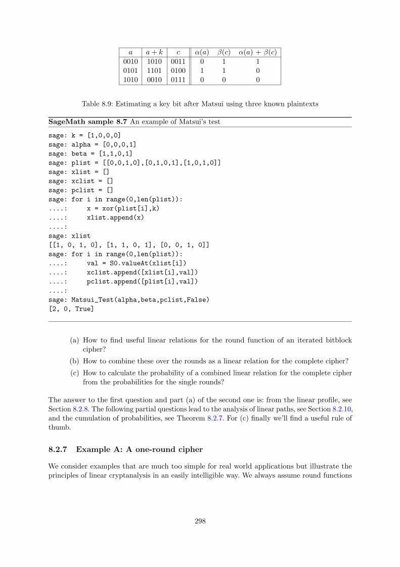
a a+ k c α(a) β(c) α(a) + β(c)
0010 1010 0011 0 1 10101 1101 0100 1 1 01010 0010 0111 0 0 0
Table 8.9: Estimating a key bit after Matsui using three known plaintexts
SageMath sample 8.7 An example of Matsui’s test
sage: k = [1,0,0,0]
sage: alpha = [0,0,0,1]
sage: beta = [1,1,0,1]
sage: plist = [[0,0,1,0],[0,1,0,1],[1,0,1,0]]
sage: xlist = []
sage: xclist = []
sage: pclist = []
sage: for i in range(0,len(plist)):
....: x = xor(plist[i],k)
....: xlist.append(x)
....:
sage: xlist
[[1, 0, 1, 0], [1, 1, 0, 1], [0, 0, 1, 0]]
sage: for i in range(0,len(plist)):
....: val = S0.valueAt(xlist[i])
....: xclist.append([xlist[i],val])
....: pclist.append([plist[i],val])
....:
sage: Matsui_Test(alpha,beta,pclist,False)
[2, 0, True]
(a) How to find useful linear relations for the round function of an iterated bitblockcipher?
(b) How to combine these over the rounds as a linear relation for the complete cipher?
(c) How to calculate the probability of a combined linear relation for the complete cipherfrom the probabilities for the single rounds?
The answer to the first question and part (a) of the second one is: from the linear profile, seeSection 8.2.8. The following partial questions lead to the analysis of linear paths, see Section 8.2.10,and the cumulation of probabilities, see Theorem 8.2.7. For (c) finally we’ll find a useful rule ofthumb.
8.2.7 Example A: A one-round cipher
We consider examples that are much too simple for real world applications but illustrate theprinciples of linear cryptanalysis in an easily intelligible way. We always assume round functions
298
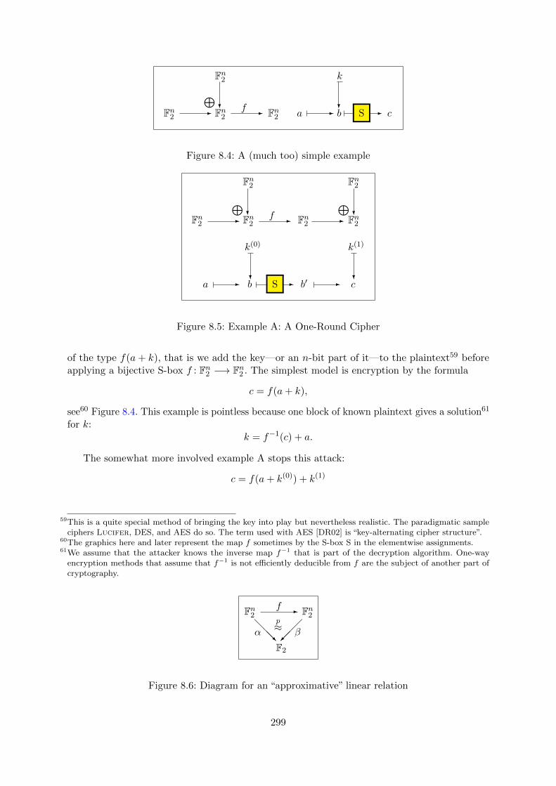
Fn2 - Fn2
⊕Fn2
?-f Fn2 a - b
k
?-S c
Figure 8.4: A (much too) simple example
Fn2 - Fn2
⊕Fn2
?-f Fn2 -
Fn2
?⊕
Fn2
a - b
k(0)
?-S b′
k(1)
?- c
Figure 8.5: Example A: A One-Round Cipher
of the type f(a+ k), that is we add the key—or an n-bit part of it—to the plaintext59 beforeapplying a bijective S-box f : Fn2 −→ Fn2 . The simplest model is encryption by the formula
c = f(a+ k),
see60 Figure 8.4. This example is pointless because one block of known plaintext gives a solution61
for k:k = f−1(c) + a.
The somewhat more involved example A stops this attack:
c = f(a+ k(0)) + k(1)
59This is a quite special method of bringing the key into play but nevertheless realistic. The paradigmatic sampleciphers Lucifer, DES, and AES do so. The term used with AES [DR02] is “key-alternating cipher structure”.
60The graphics here and later represent the map f sometimes by the S-box S in the elementwise assignments.61We assume that the attacker knows the inverse map f−1 that is part of the decryption algorithm. One-way
encryption methods that assume that f−1 is not efficiently deducible from f are the subject of another part ofcryptography.
Fn2 -f Fn2
F2
@@@R
α�
��β
p≈
Figure 8.6: Diagram for an “approximative” linear relation
299
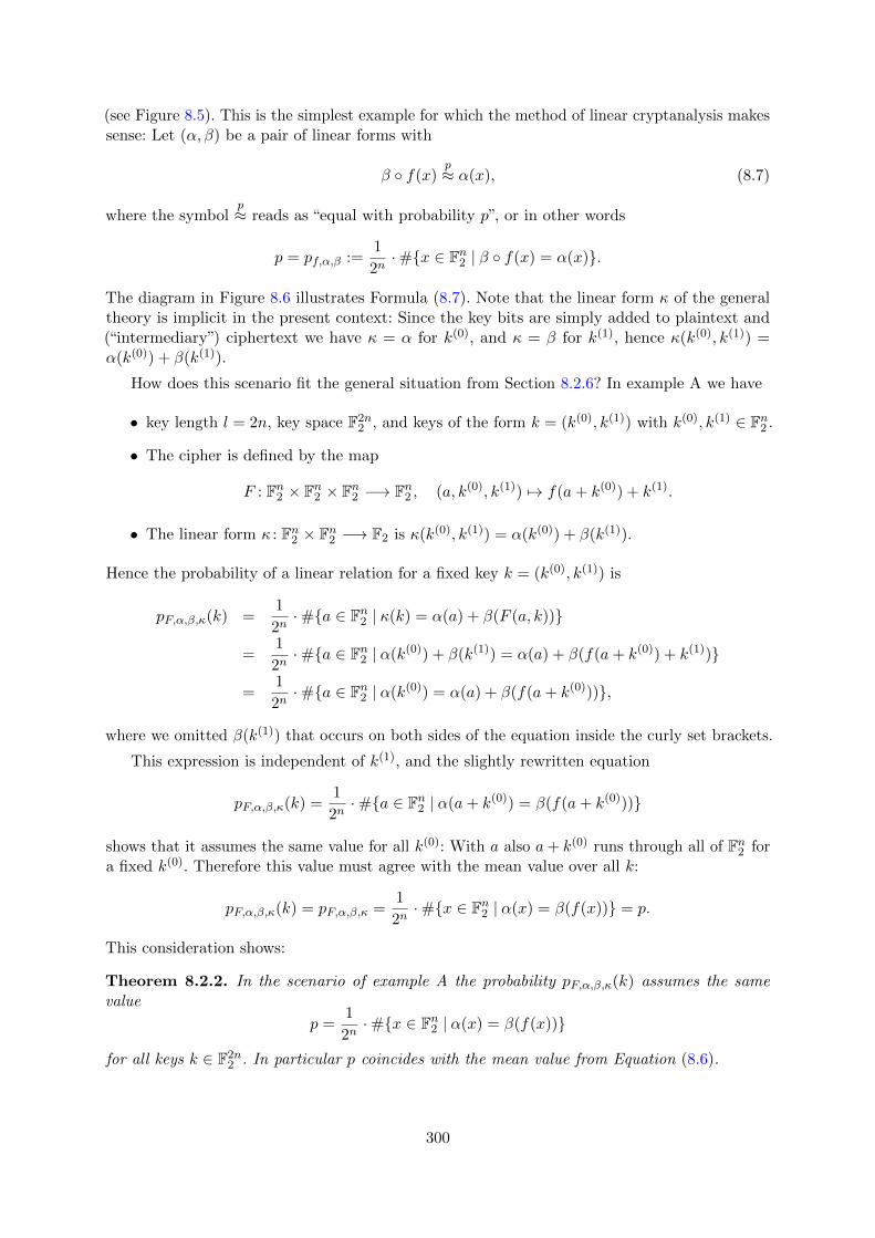
(see Figure 8.5). This is the simplest example for which the method of linear cryptanalysis makessense: Let (α, β) be a pair of linear forms with
β ◦ f(x)p≈ α(x), (8.7)
where the symbolp≈ reads as “equal with probability p”, or in other words
p = pf,α,β :=1
2n·#{x ∈ Fn2 | β ◦ f(x) = α(x)}.
The diagram in Figure 8.6 illustrates Formula (8.7). Note that the linear form κ of the generaltheory is implicit in the present context: Since the key bits are simply added to plaintext and(“intermediary”) ciphertext we have κ = α for k(0), and κ = β for k(1), hence κ(k(0), k(1)) =α(k(0)) + β(k(1)).
How does this scenario fit the general situation from Section 8.2.6? In example A we have
• key length l = 2n, key space F2n2 , and keys of the form k = (k(0), k(1)) with k(0), k(1) ∈ Fn2 .
• The cipher is defined by the map
F : Fn2 × Fn2 × Fn2 −→ Fn2 , (a, k(0), k(1)) 7→ f(a+ k(0)) + k(1).
• The linear form κ : Fn2 × Fn2 −→ F2 is κ(k(0), k(1)) = α(k(0)) + β(k(1)).
Hence the probability of a linear relation for a fixed key k = (k(0), k(1)) is
pF,α,β,κ(k) =1
2n·#{a ∈ Fn2 | κ(k) = α(a) + β(F (a, k))}
=1
2n·#{a ∈ Fn2 | α(k(0)) + β(k(1)) = α(a) + β(f(a+ k(0)) + k(1))}
=1
2n·#{a ∈ Fn2 | α(k(0)) = α(a) + β(f(a+ k(0)))},
where we omitted β(k(1)) that occurs on both sides of the equation inside the curly set brackets.
This expression is independent of k(1), and the slightly rewritten equation
pF,α,β,κ(k) =1
2n·#{a ∈ Fn2 | α(a+ k(0)) = β(f(a+ k(0)))}
shows that it assumes the same value for all k(0): With a also a+ k(0) runs through all of Fn2 fora fixed k(0). Therefore this value must agree with the mean value over all k:
pF,α,β,κ(k) = pF,α,β,κ =1
2n·#{x ∈ Fn2 | α(x) = β(f(x))} = p.
This consideration shows:
Theorem 8.2.2. In the scenario of example A the probability pF,α,β,κ(k) assumes the samevalue
p =1
2n·#{x ∈ Fn2 | α(x) = β(f(x))}
for all keys k ∈ F2n2 . In particular p coincides with the mean value from Equation (8.6).
300
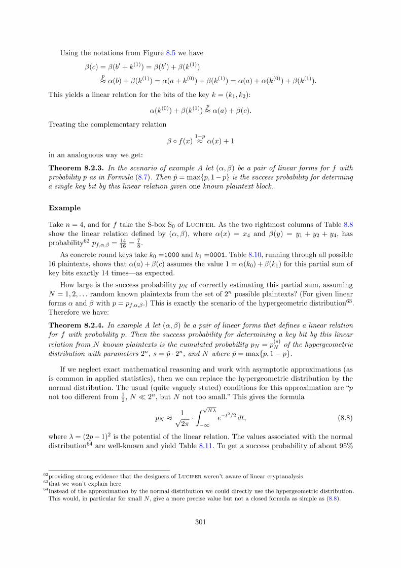
Using the notations from Figure 8.5 we have
β(c) = β(b′ + k(1)) = β(b′) + β(k(1))p≈ α(b) + β(k(1)) = α(a+ k(0)) + β(k(1)) = α(a) + α(k(0)) + β(k(1)).
This yields a linear relation for the bits of the key k = (k1, k2):
α(k(0)) + β(k(1))p≈ α(a) + β(c).
Treating the complementary relation
β ◦ f(x)1−p≈ α(x) + 1
in an analoguous way we get:
Theorem 8.2.3. In the scenario of example A let (α, β) be a pair of linear forms for f withprobability p as in Formula (8.7). Then p = max{p, 1− p} is the success probability for determinga single key bit by this linear relation given one known plaintext block.
Example
Take n = 4, and for f take the S-box S0 of Lucifer. As the two rightmost columns of Table 8.8show the linear relation defined by (α, β), where α(x) = x4 and β(y) = y1 + y2 + y4, hasprobability62 pf,α,β = 14
16 = 78 .
As concrete round keys take k0 =1000 and k1 =0001. Table 8.10, running through all possible16 plaintexts, shows that α(a) + β(c) assumes the value 1 = α(k0) + β(k1) for this partial sum ofkey bits exactly 14 times—as expected.
How large is the success probability pN of correctly estimating this partial sum, assumingN = 1, 2, . . . random known plaintexts from the set of 2n possible plaintexts? (For given linearforms α and β with p = pf,α,β .) This is exactly the scenario of the hypergeometric distribution63.Therefore we have:
Theorem 8.2.4. In example A let (α, β) be a pair of linear forms that defines a linear relationfor f with probability p. Then the success probability for determining a key bit by this linear
relation from N known plaintexts is the cumulated probability pN = p(s)N of the hypergeometric
distribution with parameters 2n, s = p · 2n, and N where p = max{p, 1− p}.
If we neglect exact mathematical reasoning and work with asymptotic approximations (asis common in applied statistics), then we can replace the hypergeometric distribution by thenormal distribution. The usual (quite vaguely stated) conditions for this approximation are “pnot too different from 1
2 , N � 2n, but N not too small.” This gives the formula
pN ≈1√2π·∫ √Nλ−∞
e−t2/2 dt, (8.8)
where λ = (2p− 1)2 is the potential of the linear relation. The values associated with the normaldistribution64 are well-known and yield Table 8.11. To get a success probability of about 95%
62providing strong evidence that the designers of Lucifer weren’t aware of linear cryptanalysis63that we won’t explain here64Instead of the approximation by the normal distribution we could directly use the hypergeometric distribution.
This would, in particular for small N , give a more precise value but not a closed formula as simple as (8.8).
301

a b b′ c α(a) + β(c)
0000 1000 0010 0011 10001 1001 0110 0111 10010 1010 0011 0010 00011 1011 0001 0000 10100 1100 1001 1000 10101 1101 0100 0101 10110 1110 0101 0100 10111 1111 1000 1001 11000 0000 1100 1101 11001 0001 1111 1110 11010 0010 0111 0110 11011 0011 1010 1011 11100 0100 1110 1111 11101 0101 1101 1100 11110 0110 1011 1010 11111 0111 0000 0001 0
Table 8.10: A linear relation for the key bits (b arises from a by adding k(0), resulting in “flipping”the first bit, b′ from b by applying f , and c from b′ by adding k(1).
Nλ 1 2 3 4 . . . 8 9pN 84, 1% 92, 1% 95, 8% 97, 7% . . . 99, 8% 99, 9%
Table 8.11: Dependence of the success probability on the number of known plaintexts
we need N ≈ 3λ known plaintexts according to the table. In the concrete example above we had
p = 78 , hence λ = 9
16 , and the number of known plaintexts needed for a 95% success probabilityis N ≈ 5. Using Table 8.9 we succeeded with only N = 3 plaintexts. This is no great surprisebecause the a-priori probability of this success is about 90% (for Nλ = 27
16 ≈ 1, 68 . . .)65.
8.2.8 Approximation Table, Correlation Matrix, and Linear Profile
Linear relations for a Boolean map (or S-box) f: Fn2 −→ Fq2 are true with certain frequencies (orprobabilities). We collect these frequencies in a matrix of size 2n×2q, called the approximationtable66 of f . This table gives, for each pair (α, β) of linear forms, the number of arguments xwhere β ◦ f(x) = α(x). Table 8.12 shows the approximation table of the S-box S0 of Lucifer.The entry 16 in the upper left corner says that the relation 0 = 0 is true in all 16 possible cases.At the same time 16 is the common denominator by which we have to divide all other entriesto get the probabilities. In the general case the upper left corner would be 2n. The remaining
65Here the condition “N not too small” for the approximation by the normal distribution is more than arguable.However determining the exact values for the hypergeometric distribution is easy: Consider an urn containing 16balls, 14 black ones and 2 white ones, and draw 3 balls by random. Then the probability of all of them beingblack is 26
40, the probability of two being black and one being white is 13
40. Hence the probability of at least two
balls being black is 3940
= 97, 5%. This is clearly more than the 90% from the approximation (8.8). The remainingprobabilities are 1
40for exactly one black ball, and 0 for three white balls.
66When using references be aware that often all entries are diminished by 2n−1, for example by the SageMathfunction linear_approximation_matrix().
302
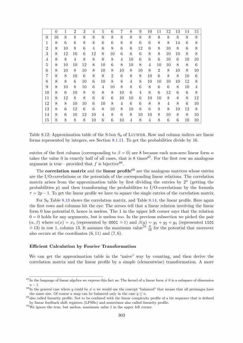
0 1 2 3 4 5 6 7 8 9 10 11 12 13 14 15
0 16 8 8 8 8 8 8 8 8 8 8 8 8 8 8 81 8 6 6 8 8 6 6 8 8 6 6 8 8 14 6 82 8 10 8 6 4 6 8 6 6 12 6 8 10 8 6 83 8 12 10 6 12 8 10 6 6 6 8 8 10 10 8 84 8 8 4 8 8 8 8 4 10 6 6 6 10 6 10 105 8 10 10 12 8 10 6 8 10 8 4 10 10 8 8 66 8 10 8 10 8 10 8 10 8 10 8 2 8 10 8 107 8 8 10 6 8 8 2 6 8 8 10 6 8 8 10 68 8 8 6 10 6 10 8 8 4 8 10 10 10 10 12 89 8 10 8 10 6 4 10 8 8 6 8 6 6 8 10 410 8 6 10 8 6 8 8 10 6 4 8 6 12 6 6 811 8 12 8 8 6 6 6 10 10 6 10 10 8 8 8 1212 8 8 10 10 6 10 8 4 6 6 8 8 4 8 6 1013 8 6 12 6 6 8 10 8 10 8 6 8 8 10 12 814 8 6 10 12 10 4 8 6 8 10 10 8 10 8 8 1015 8 8 8 8 10 6 6 10 4 8 4 8 6 6 10 10
Table 8.12: Approximation table of the S-box S0 of Lucifer. Row and column indices are linearforms represented by integers, see Section 8.1.11. To get the probabilities divide by 16.
entries of the first column (corresponding to β = 0) are 8 because each non-zero linear form αtakes the value 0 in exactly half of all cases, that is 8 times67. For the first row an analogousargument is true—provided that f is bijective68.
The correlation matrix and the linear profile69 are the analogous matrices whose entriesare the I/O-correlations or the potentials of the corresponding linear relations. The correlationmatrix arises from the approximation table by first dividing the entries by 2n (getting theprobabilities p) and then transforming the probabilities to I/O-correlations by the formulaτ = 2p− 1. To get the linear profile we have to square the single entries of the correlation matrix.
For S0 Table 8.13 shows the correlation matrix, and Table 8.14, the linear profile. Here againthe first rows and columns hit the eye: The zeroes tell that a linear relation involving the linearform 0 has potential 0, hence is useless. The 1 in the upper left corner says that the relation0 = 0 holds for any arguments, but is useless too. In the previous subsection we picked the pair(α, β) where α(x) = x4 (represented by 0001 = 1) and β(y) = y1 + y2 + y4 (represented 1101
= 13) in row 1, column 13. It assumes the maximum value70 916 for the potential that moreover
also occurs at the coordinates (6, 11) and (7, 6).
Efficient Calculation by Fourier Transformation
We can get the approximation table in the “naive” way by counting, and then derive thecorrelation matrix and the linear profile by a simple (elementwise) transformation. A more
67In the language of linear algebra we express this fact as: The kernel of a linear form 6= 0 is a subspace of dimensionn− 1.
68In the general case where q could be 6= n we would use the concept “balanced” that means that all preimages havethe same size. Of course a map can be balanced only in the case q ≤ n.
69also called linearity profile. Not to be confused with the linear complexity profile of a bit sequence that is definedby linear feedback shift registers (LFSRs) and sometimes also called linearity profile.
70We ignore the true, but useless, maximum value 1 in the upper left corner.
303
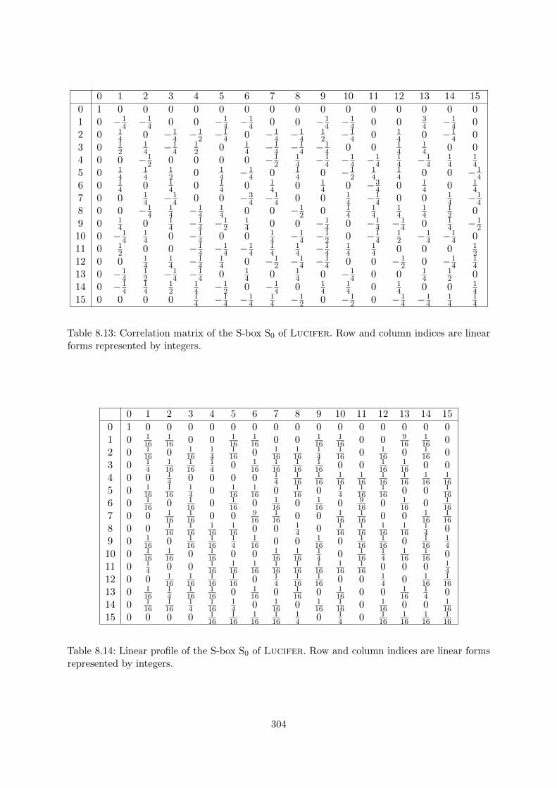
0 1 2 3 4 5 6 7 8 9 10 11 12 13 14 15
0 1 0 0 0 0 0 0 0 0 0 0 0 0 0 0 01 0 −1
4 −14 0 0 −1
4 −14 0 0 −1
4 −14 0 0 3
4 −14 0
2 0 14 0 −1
4 −12 −1
4 0 −14 −1
412 −1
4 0 14 0 −1
4 03 0 1
214 −1
412 0 1
4 −14 −1
4 −14 0 0 1
414 0 0
4 0 0 −12 0 0 0 0 −1
214 −1
4 −14 −1
414 −1
414
14
5 0 14
14
12 0 1
4 −14 0 1
4 0 −12
14
14 0 0 −1
46 0 1
4 0 14 0 1
4 0 14 0 1
4 0 −34 0 1
4 0 14
7 0 0 14 −1
4 0 0 −34 −1
4 0 0 14 −1
4 0 0 14 −1
48 0 0 −1
414 −1
414 0 0 −1
2 0 14
14
14
14
12 0
9 0 14 0 1
4 −14 −1
214 0 0 −1
4 0 −14 −1
4 0 14 −1
210 0 −1
414 0 −1
4 0 0 14 −1
4 −12 0 −1
412 −1
4 −14 0
11 0 12 0 0 −1
4 −14 −1
414
14 −1
414
14 0 0 0 1
212 0 0 1
414 −1
414 0 −1
2 −14 −1
4 0 0 −12 0 −1
414
13 0 −14
12 −1
4 −14 0 1
4 0 14 0 −1
4 0 0 14
12 0
14 0 −14
14
12
14 −1
2 0 −14 0 1
414 0 1
4 0 0 14
15 0 0 0 0 14 −1
4 −14
14 −1
2 0 −12 0 −1
4 −14
14
14
Table 8.13: Correlation matrix of the S-box S0 of Lucifer. Row and column indices are linearforms represented by integers.
0 1 2 3 4 5 6 7 8 9 10 11 12 13 14 15
0 1 0 0 0 0 0 0 0 0 0 0 0 0 0 0 01 0 1
16116 0 0 1
16116 0 0 1
16116 0 0 9
16116 0
2 0 116 0 1
1614
116 0 1
16116
14
116 0 1
16 0 116 0
3 0 14
116
116
14 0 1
16116
116
116 0 0 1
16116 0 0
4 0 0 14 0 0 0 0 1
4116
116
116
116
116
116
116
116
5 0 116
116
14 0 1
16116 0 1
16 0 14
116
116 0 0 1
166 0 1
16 0 116 0 1
16 0 116 0 1
16 0 916 0 1
16 0 116
7 0 0 116
116 0 0 9
16116 0 0 1
16116 0 0 1
16116
8 0 0 116
116
116
116 0 0 1
4 0 116
116
116
116
14 0
9 0 116 0 1
16116
14
116 0 0 1
16 0 116
116 0 1
1614
10 0 116
116 0 1
16 0 0 116
116
14 0 1
1614
116
116 0
11 0 14 0 0 1
16116
116
116
116
116
116
116 0 0 0 1
412 0 0 1
16116
116
116 0 1
4116
116 0 0 1
4 0 116
116
13 0 116
14
116
116 0 1
16 0 116 0 1
16 0 0 116
14 0
14 0 116
116
14
116
14 0 1
16 0 116
116 0 1
16 0 0 116
15 0 0 0 0 116
116
116
116
14 0 1
4 0 116
116
116
116
Table 8.14: Linear profile of the S-box S0 of Lucifer. Row and column indices are linear formsrepresented by integers.
304
efficient algorithm uses the Fourier71 transformation. In the binary case it is especially simple,and due to historically independent inventions is also called Hadamard72 transformation, orWalsh73 transformation. It transforms a real valued (!) function ϕ : Fm2 −→ R into another realvalued function ϕ : Fm2 −→ R defined by74
ϕ(u) :=∑x∈Fm2
ϕ(x) · (−1)u·x.
Here u ·x is the canonical scalar product in Fm2 . The exponents are not integers but bits, howeverthis is OK since over the basis −1 for integer exponents only the residue classes modulo 2 matter.
Now consider a Boolean map f : Fn2 −→ Fq2 and its indicator function ϑf : Fn2 × Fq2 −→ R,
ϑf (x, y) :=
{1, if y = f(x),0 else.
Let us calculate its Fourier transform; set m = n+ q and split the variables into blocks of lengthsn and q:
ϑf (u, v) =∑x∈Fn2
∑y∈Fq2
ϑf (x, y)(−1)u·x+v·y
=∑x∈Fn2
(−1)u·x+v·f(x).
In the exponent we see the linear forms x 7→ u ·x on Fn2 that we denote by α, and y 7→ v · y on Fq2that we denote by β. Then u is the bitblock representation of α, and v, of β, and the exponent is
α(x) + β ◦ f(x).
an expression familiar from linear cryptanalysis. If α(x) = β ◦ f(x), then the exponent is 0, hencethe summand is 1. Otherwise the exponent is 1, the summand is −1. Thus we sum up 2n · pf,α,βones and 2n − 2n · pf,α,β “minus ones”, and the sum is
2n · [pf,α,β − (1− pf,α,β)] = 2n · τf,α,β .
Hence ϑf (u, v) is the I/O-correlation of (α, β) up to a normalizing factor 2n.
The Fourier transform ϑf : Fn2 × Fq2 −→ R of the indicator function of a Boolean mapf: Fn2 −→ Fq2 is called the (Walsh-) spectrum of f . We have shown:
Theorem 8.2.5. The spectrum of a Boolean map f : Fn2 −→ Fq2 coincides with 2n times thecorrelation matrix.
This theorem is of eminent theoretical and practical importance:
• On the theoretical side it leads to very elegant and short proofs of statements about thecorrelation matrix and related objects [Pom14].
71Joseph Fourier, French mathematician and physicist, March 21, 1768 – May 16, 183072Jacques Hadamard, French mathematician, December 8, 1865 – October 17, 196373Joseph L. Walsh, American mathematician, September 21, 1895 – December 6, 197374This is a special case of the discrete Fourier transformation. In the general case we would use the complex N -th
root of unity ζ = e2πi/N instead of −1, and transform complex valued functions over the ring Z/NZ, instead overF2 = Z/2Z—or functions on Zm that have period N in each of the variables. In the binary case N = 2, and the2nd root of unity −1 is real, so we only need to consider real valued functions.
305

• On the practical side it allows the calculation of the correlation matrix (and consequentlyalso of the approximation table and of the linear profile) by the fast Fourier transformation75
that drops the cost by a factor of (essentially) 2n using binary recursion.
How large is the net effect of FFT? For simplicity we only consider the case n = q. The naiveprocedure counts 2n arguments in determining pf,α,β (and thereby also τf,α,β) for fixed α and β,the map being given by the value table. Hence the total cost is 2n · 2n · 2n.
We won’t explain the FFT (see [Pom14]). It is at the heart of the function wtr() fromAppendix 8.4.5. We remark without proof that the FFT of a real valued function Fm2 −→ R takes3m · 2m simple operations with real numbers that we may count in the naive way for functionswith values in {−1, 1} noting that the calculation involves only integers of moderate size. Thismakes a total of 3 · 2n · 22n operations.
The fair way to describe the cost of an algorithm is as function of the size N of its input.Here the input is the value table of a Boolean map Fn2 −→ Fn2 . Hence N = n · 2n—the valuetable describes n component functions each at 2n arguments. From this point of view the cost ofthe naive algorithm is (essentially) cubic, the cost of the fast algorithm (essentially) quadratic.
Anyway the cryptologist’s preferred parameter is block length. From this point of view thecost grows exponentially in both cases although with a different rate. By the fast algorithm thecalculation is feasible for “small” S-boxes, say up to a block length of 10.
SageMath sample 8.8 shows the calculation of the correlation matrix, the approximationtable76, and the linear profile of S0. (Remember to divide the entries of the resulting matrixSpec by 16, those of linProf by 256.)
SageMath sample 8.8 Correlation matrix, approximation table, and linear profile of the S-boxS0
sage: Spec = S0.wspec()
sage: ApprT = S0.linApprTable()
sage: linProf = S0.linProf()
If we call the method linProf() with the additional parameter extended=True, as inSageMath sample 8.9, then it outputs the maximal entry, as well as all index pairs where itoccurs. A look at the approximation table or the correlation matrix then shows whether thecorresponding linear relation has probability larger or smaller than 1
2 , specifying whether theresulting bit has to be complemented.
8.2.9 Example B: A two-round cipher
As a next step we iterate the round map
f : Fn2 × Fq2 −→ Fn2of a bitblock cipher over two rounds using round keys k(i) ∈ Fq2 as illustrated in Figure 8.777.
We consider linear relations
κ1(k(1))
p1≈ α1(c(0)) + β1(c
(1))
75abbreviated as FFT76For calculating the approximation table the SageMath class sage.crypto.mq.sbox.SBox of-
fers the function S0.linear_approximation_matrix() where the S-box has the definition S0 =
306

SageMath sample 8.9 Linear profile of the S-box S0 with evaluation
sage: lProf = S0.linProf(extended=True)
sage: lProf[0]
[...]
sage: print("Maximum entry:", lProf[1], "| with denominator:", lProf[2])
(’Maximum entry:’, 144, ’| with denominator:’, 256)
sage: print("at indices:", lProf[3])
(’at indices:’, [[1, 13], [6, 11], [7, 6]])
sage: Spec = S0.wspec()
sage: for coord in lProf[3]:
....: if (Spec[coord[0]][coord[1]] < 0):
....: print ("For relation at", coord, "take complement.")
....:
(’For relation at’, [6, 11], ’take complement.’)
(’For relation at’, [7, 6], ’take complement.’)
with probability p1, I/O-correlation τ1 = 2p1 − 1, and potential λ1 = τ21 , and
κ2(k(2))
p2≈ α2(c(1)) + β2(c
(2))
with probability p2, I/O-correlation τ2 = 2p2 − 1, and potential λ2 = τ22 . We can combine thesetwo linear relations if α2 = β1, thereby getting a linear relation for some key bits expressed bythe (known) plaintext c(0) = a and the ciphertext c(2) = c,
κ1(k(1)) + κ2(k
(2))p≈ α1(c
(0)) + β2(c(2)),
that holds with a certain probability p, and has I/O-correlation τ and potential λ, that in generaldepend on k = (k(1), k(2)) and are difficult to determine. Therefore we again consider a simplifiedexample B, see Figure 8.8. Encryption is done step by step by the formulas
b(0) = a+ k(0), a(1) = f1(b(0)), b(1) = a(1) + k(1), a(2) = f2(b
(1)), c = a(2) + k(2).
(Here f1 is given by the S-box S0, and f2, by the S-box S1 that could be identical with S078.) As
for example A adding some key bits after the last round prevents the “stripping off” of f2.
Comparing example B with the general settings in Section 8.2.6 we have:
• key length l = 3n, key space F3n2 , and keys of the form k = (k(0), k(1), k(2)) with
k(0), k(1), k(2) ∈ Fn2 .
• Encryption is defined by the map
F : Fn2 × Fn2 × Fn2 × Fn2 −→ Fn2 ,(a, k(0), k(1), k(2)) 7→ f2(f1(a+ k(0)) + k(1)) + k(2).
mq.SBox(12,15,7,10,14,13,11,0,2,6,3,1,9,4,5,8). Warning: see the footnote on page 302.77In a certain sense example A already was a two-round cipher since we used two partial keys. Adding one more
S-box at the right side of Figure 8.5 would be cryptologically irrelevant, because this non-secret part of thealgorithm would be known to the cryptanalyst who simply could “strip it off” (that is, apply its inverse to thecipher text) and be left with example A. In a similar way we could interpret example B as a three-round cipher.However this would be a not so common counting of rounds.
78We allow that the round functions of the different rounds differ. The reason is that usually the round functionconsists of several parallel S-boxes and the permutations direct an input bit through different S-boxes on its waythrough the rounds, see Section 8.2.12.
307

a = c(0)
?f� ��� k(1)
?
f(c(0), k(1)) = c(1)
?f� ��� k(2)
?
c = f(c(1), k(2)) = c(2)
linear relation (α1, β1, κ1)
with κ1(k(1))
p1≈ α1(c(0)) + β1(c
(1))
linear relation (α2, β2, κ2)
with κ2(k(2))
p2≈ α2(c(1)) + β2(c
(2))
Figure 8.7: General two-round cipher
• The linear form κ: Fn2 × Fn2 × Fn2 −→ F2 is given by
κ(k(0), k(1), k(2)) = α(k(0)) + β(k(1)) + γ(k(2)).
Here (α, β) is a linear relation for f1 with probability p1, I/O-correlation τ1, and potential λ1,and (β, γ), a linear relation for f2 with probability p2, I/O-correlation τ2, and potential λ2 (thesame β since we want to combine the linear relations), where
p1 =1
2n·#{x ∈ Fn2 | β ◦ f1(x) = α(x)}
p2 =1
2n·#{y ∈ Fn2 | γ ◦ f2(y) = β(y)}
With the notations of Figure 8.8 we have
γ(c) = γ(a(2)) + γ(k(2))p2≈ β(b(1)) + γ(k(2)) = β(a(1)) + β(k(1)) + γ(k(2))
p1≈ α(b(0)) + β(k(1)) + γ(k(2)) = α(a) + α(k(0)) + β(k(1)) + γ(k(2))
Hence we get a linear relation for the key bits as a special case of Equation (8.5) in the form
α(k(0)) + β(k(1)) + γ(k(2))p≈ α(a) + γ(c)
with a certain probability p that is defined by the formula
p = pF,α,β,γ(k)
=1
2n·#{a ∈ Fn2 | α(k(0)) + β(k(1)) + γ(k(2)) = α(a) + γ(F (a, k))}.
We try to explicitly determine p. As for the one-round case we first ask how p depends on k.Insert the definition of F (a, k) into the defining equation inside the set brackets. Then γ(k(2))cancels out and we are left with
pF,α,β,γ(k) =1
2n·#{a ∈ Fn2 | α(k(0) + a) + β(k(1)) = γ(f2(k
(1) + f1(k(0) + a)))}.
308

Fn2 - Fn2
⊕Fn2
?-f1 Fn2 -
Fn2
?⊕
Fn2 -f2 Fn2 -
Fn2
?⊕
Fn2
F2
@@@R
α�
��β
p1≈
F2
@@@R
β�
��γ
p2≈
a - b(0)
k(0)
?-S0 a(1)
k(1)
?- b(1) -S1 a(2)
k(2)
?- c
Figure 8.8: Example B: a two-round cipher
This is independent of k(2), and for all k(0) assumes the same value
pF,α,β,γ(k) =1
2n·#{x ∈ Fn2 | α(x) = β(k(1)) + γ(f2(k
(1) + f1(x)))}
because x = k(0) + a runs through Fn2 along with a. This value indeed depends on k, but only onthe middle component k(1). Now form the mean value p := pF,α,β,γ over all keys:
p =1
22n·#{(x, k(1)) ∈ F2n
2 | α(x) = β(k(1)) + γ(f2(k(1) + f1(x)))}.
Inside the brackets we see the expression γ(f2(k(1) + f1(x))), and we know:
γ(f2(k(1) + f1(x))) =
{β(k(1) + f1(x)) with probability p2,
1 + β(k(1) + f1(x)) with probability 1− p2.
Here “probability p2” means that the statement is true for p2 · 22n of all possible (x, k(1)) ∈ F2n2 .
Substituting this we get
p =1
22n·[p2 ·#{(x, k(1)) ∈ F2n
2 | α(x) = β(f1(x))}
+(1− p2) ·#{(x, k(1)) ∈ F2n2 | α(x) 6= β(f1(x))}
]where now the defining equations of both sets are also independent of k(1). We recognize thedefinition of p1 and substitute it getting
p = p1p2 + (1− p1)(1− p2) = 2p1p2 − p1 − p2 + 1.
This formula looks much more beautiful if expressed in terms of the I/O-correlations τ = 2p− 1and τi = 2pi − 1 for i = 1 and 2:
τ = 2p− 1 = 4p1p2 − 2p1 − 2p2 + 1 = (2p1 − 1)(2p2 − 1) = τ1τ2.
In summary we have proved:
309

a b(0) a(1) b(1) a(2) c β(b(1)) γ(a(2)) α(a) + γ(c)
0000 1000 0010 0011 1001 1111 1 1 00001 1001 0110 0111 0100 0010 0 1 10010 1010 0011 0010 1110 1000 0 0 10011 1011 0001 0000 0111 0001 0 1 10100 1100 1001 1000 1100 1010 1 0 10101 1101 0100 0101 1011 1101 0 1 10110 1110 0101 0100 0011 0101 1 0 10111 1111 1000 1001 1101 1011 0 0 01000 0000 1100 1101 1111 1001 1 0 11001 0001 1111 1110 1000 1110 0 1 11010 0010 0111 0110 0000 0110 1 0 11011 0011 1010 1011 1010 1100 0 1 11100 0100 1110 1111 0101 0011 1 1 01101 0101 1101 1100 0110 0000 0 1 11110 0110 1011 1010 0001 0111 1 0 11111 0111 0000 0001 0010 0100 1 0 0
Table 8.15: The data flow in the concrete example for B, and some linear forms
Theorem 8.2.6. For example B we have:
(i) The probability pF,α,β,γ(k) depends only on the middle component k(1) of the key k =(k(0), k(1), k(2)) ∈ Fn2 × Fn2 × Fn2 .
(ii) The mean value of these probabilities over all keys k is pF,α,β,γ = p = 2p1p2 − p1 − p2 + 1.
(iii) The I/O-correlations and the potentials are multiplicative:
τF,α,β,γ = τ1τ2 and λF,α,β,γ = λ1λ2.
In Matsui’s test we face the decision whether to use the linear relation or its negation forestimating a bit. We can’t do better than use the mean value pF,α,β,γ since the key and the trueprobability pF,α,β,γ(k) are unknown. This could be an error since these two probabilities mightlie on different sides of 1
2 .
SageMath sample 8.10 A Boolean map (S-box S1 of Lucifer)
g1 = BoolF([0,0,1,1,0,1,0,0,1,1,0,1,0,1,1,0])
g2 = BoolF([1,0,1,0,0,0,0,1,1,1,0,0,1,1,0,1])
g3 = BoolF([1,1,1,0,1,1,0,0,0,0,0,1,1,1,0,0])
g4 = BoolF([1,0,0,1,1,1,0,0,0,1,1,0,0,1,0,1])
S1 = BoolMap([g1,g2,g3,g4])
Example
Let n = 4, S0 as in 8.2.7, and S1 as defined in SageMath sample 8.1079 and as given in Table 8.15(in different order) as transition from column b(1) to column a(2). (This table is easily calculated
79By the way this is the second S-box of Lucifer.
310
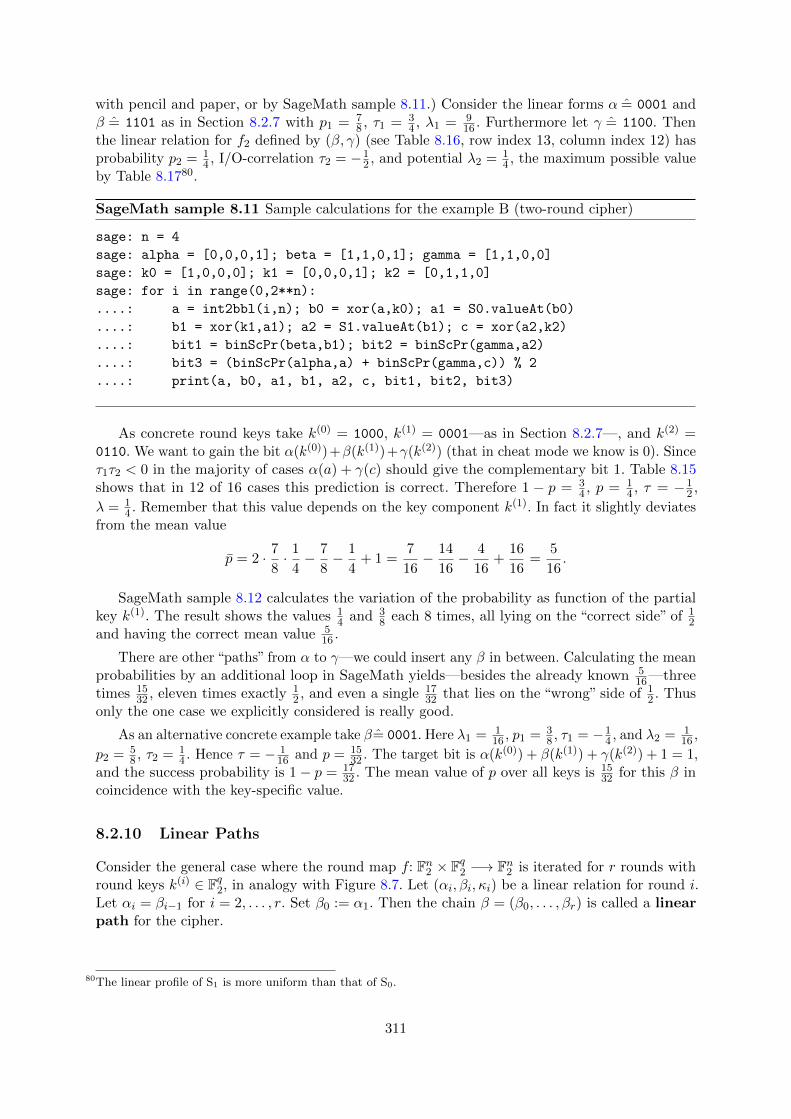
with pencil and paper, or by SageMath sample 8.11.) Consider the linear forms α = 0001 andβ = 1101 as in Section 8.2.7 with p1 = 7
8 , τ1 = 34 , λ1 = 9
16 . Furthermore let γ = 1100. Thenthe linear relation for f2 defined by (β, γ) (see Table 8.16, row index 13, column index 12) hasprobability p2 = 1
4 , I/O-correlation τ2 = −12 , and potential λ2 = 1
4 , the maximum possible valueby Table 8.1780.
SageMath sample 8.11 Sample calculations for the example B (two-round cipher)
sage: n = 4
sage: alpha = [0,0,0,1]; beta = [1,1,0,1]; gamma = [1,1,0,0]
sage: k0 = [1,0,0,0]; k1 = [0,0,0,1]; k2 = [0,1,1,0]
sage: for i in range(0,2**n):
....: a = int2bbl(i,n); b0 = xor(a,k0); a1 = S0.valueAt(b0)
....: b1 = xor(k1,a1); a2 = S1.valueAt(b1); c = xor(a2,k2)
....: bit1 = binScPr(beta,b1); bit2 = binScPr(gamma,a2)
....: bit3 = (binScPr(alpha,a) + binScPr(gamma,c)) % 2
....: print(a, b0, a1, b1, a2, c, bit1, bit2, bit3)
As concrete round keys take k(0) = 1000, k(1) = 0001—as in Section 8.2.7—, and k(2) =0110. We want to gain the bit α(k(0))+β(k(1))+γ(k(2)) (that in cheat mode we know is 0). Sinceτ1τ2 < 0 in the majority of cases α(a) + γ(c) should give the complementary bit 1. Table 8.15shows that in 12 of 16 cases this prediction is correct. Therefore 1 − p = 3
4 , p = 14 , τ = −1
2 ,
λ = 14 . Remember that this value depends on the key component k(1). In fact it slightly deviates
from the mean value
p = 2 · 7
8· 1
4− 7
8− 1
4+ 1 =
7
16− 14
16− 4
16+
16
16=
5
16.
SageMath sample 8.12 calculates the variation of the probability as function of the partialkey k(1). The result shows the values 1
4 and 38 each 8 times, all lying on the “correct side” of 1
2and having the correct mean value 5
16 .
There are other “paths” from α to γ—we could insert any β in between. Calculating the meanprobabilities by an additional loop in SageMath yields—besides the already known 5
16—threetimes 15
32 , eleven times exactly 12 , and even a single 17
32 that lies on the “wrong” side of 12 . Thus
only the one case we explicitly considered is really good.
As an alternative concrete example take β= 0001. Here λ1 = 116 , p1 = 3
8 , τ1 = −14 , and λ2 = 1
16 ,
p2 = 58 , τ2 = 1
4 . Hence τ = − 116 and p = 15
32 . The target bit is α(k(0)) + β(k(1)) + γ(k(2)) + 1 = 1,and the success probability is 1− p = 17
32 . The mean value of p over all keys is 1532 for this β in
coincidence with the key-specific value.
8.2.10 Linear Paths
Consider the general case where the round map f: Fn2 × Fq2 −→ Fn2 is iterated for r rounds withround keys k(i) ∈ Fq2, in analogy with Figure 8.7. Let (αi, βi, κi) be a linear relation for round i.Let αi = βi−1 for i = 2, . . . , r. Set β0 := α1. Then the chain β = (β0, . . . , βr) is called a linearpath for the cipher.
80The linear profile of S1 is more uniform than that of S0.
311

0 1 2 3 4 5 6 7 8 9 10 11 12 13 14 15
0 16 8 8 8 8 8 8 8 8 8 8 8 8 8 8 81 8 10 8 10 8 6 12 10 10 4 6 8 10 8 10 82 8 6 4 10 6 8 6 8 8 10 4 6 10 8 10 83 8 8 8 8 6 6 6 6 10 6 6 10 4 8 8 124 8 8 8 4 8 8 8 4 6 6 6 10 10 10 10 65 8 6 8 10 4 6 8 6 8 6 12 6 8 10 8 66 8 10 12 10 6 12 6 8 10 8 6 8 8 10 8 67 8 8 8 12 10 10 10 6 4 8 8 8 6 10 10 108 8 8 6 10 10 6 8 8 10 10 8 12 8 12 6 69 8 6 6 8 6 12 8 10 8 6 10 12 10 8 8 1010 8 6 6 8 12 10 6 8 10 4 8 6 6 8 8 611 8 4 10 10 8 8 10 6 8 8 6 10 8 4 6 612 8 8 6 6 6 10 12 8 8 8 6 6 6 10 4 813 8 10 6 8 6 8 8 10 6 8 8 10 4 6 10 414 8 10 6 8 8 10 10 4 12 10 10 8 8 6 10 815 8 4 10 6 8 8 10 10 10 10 8 8 6 10 12 8
Table 8.16: Approximation table of the S-box S1 of Lucifer. Row and column indices are linearforms represented by integers, see Section 8.1.11. For the probabilities divide by 16.
0 1 2 3 4 5 6 7 8 9 10 11 12 13 14 15
0 1 0 0 0 0 0 0 0 0 0 0 0 0 0 0 01 0 1
16 0 116 0 1
1614
116
116
14
116 0 1
16 0 116 0
2 0 116
14
116
116 0 1
16 0 0 116
14
116
116 0 1
16 03 0 0 0 0 1
16116
116
116
116
116
116
116
14 0 0 1
44 0 0 0 1
4 0 0 0 14
116
116
116
116
116
116
116
116
5 0 116 0 1
1614
116 0 1
16 0 116
14
116 0 1
16 0 116
6 0 116
14
116
116
14
116 0 1
16 0 116 0 0 1
16 0 116
7 0 0 0 14
116
116
116
116
14 0 0 0 1
16116
116
116
8 0 0 116
116
116
116 0 0 1
16116 0 1
4 0 14
116
116
9 0 116
116 0 1
1614 0 1
16 0 116
116
14
116 0 0 1
1610 0 1
16116 0 1
4116
116 0 1
1614 0 1
16116 0 0 1
1611 0 1
4116
116 0 0 1
16116 0 0 1
16116 0 1
4116
116
12 0 0 116
116
116
116
14 0 0 0 1
16116
116
116
14 0
13 0 116
116 0 1
16 0 0 116
116 0 0 1
1614
116
116
14
14 0 116
116 0 0 1
16116
14
14
116
116 0 0 1
16116 0
15 0 14
116
116 0 0 1
16116
116
116 0 0 1
16116
14 0
Table 8.17: Linear profile of the S-box S1 of Lucifer. Row and column indices are linear formsrepresented by integers.
312
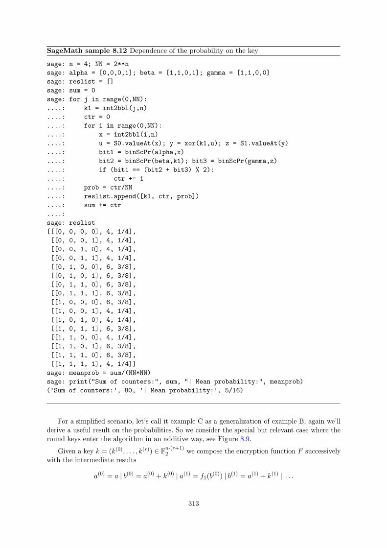
SageMath sample 8.12 Dependence of the probability on the key
sage: n = 4; NN = 2**n
sage: alpha = [0,0,0,1]; beta = [1,1,0,1]; gamma = [1,1,0,0]
sage: reslist = []
sage: sum = 0
sage: for j in range(0,NN):
....: k1 = int2bbl(j,n)
....: ctr = 0
....: for i in range(0,NN):
....: x = int2bbl(i,n)
....: u = S0.valueAt(x); y = xor(k1,u); z = S1.valueAt(y)
....: bit1 = binScPr(alpha,x)
....: bit2 = binScPr(beta,k1); bit3 = binScPr(gamma,z)
....: if (bit1 == (bit2 + bit3) % 2):
....: ctr += 1
....: prob = ctr/NN
....: reslist.append([k1, ctr, prob])
....: sum += ctr
....:
sage: reslist
[[[0, 0, 0, 0], 4, 1/4],
[[0, 0, 0, 1], 4, 1/4],
[[0, 0, 1, 0], 4, 1/4],
[[0, 0, 1, 1], 4, 1/4],
[[0, 1, 0, 0], 6, 3/8],
[[0, 1, 0, 1], 6, 3/8],
[[0, 1, 1, 0], 6, 3/8],
[[0, 1, 1, 1], 6, 3/8],
[[1, 0, 0, 0], 6, 3/8],
[[1, 0, 0, 1], 4, 1/4],
[[1, 0, 1, 0], 4, 1/4],
[[1, 0, 1, 1], 6, 3/8],
[[1, 1, 0, 0], 4, 1/4],
[[1, 1, 0, 1], 6, 3/8],
[[1, 1, 1, 0], 6, 3/8],
[[1, 1, 1, 1], 4, 1/4]]
sage: meanprob = sum/(NN*NN)
sage: print("Sum of counters:", sum, "| Mean probability:", meanprob)
(’Sum of counters:’, 80, ’| Mean probability:’, 5/16)
For a simplified scenario, let’s call it example C as a generalization of example B, again we’llderive a useful result on the probabilities. So we consider the special but relevant case where theround keys enter the algorithm in an additive way, see Figure 8.9.
Given a key k = (k(0), . . . , k(r)) ∈ Fn·(r+1)2 we compose the encryption function F successively
with the intermediate results
a(0) = a | b(0) = a(0) + k(0) | a(1) = f1(b(0)) | b(1) = a(1) + k(1) | . . .
313

Fn2 - Fn2
⊕Fn2
?-f1 Fn2 - . . . -
Fn2
?⊕
Fn2 -fr Fn2 -
Fn2
?⊕
Fn2
F2
@@@R
β0�
��β1
p1≈
F2
@@@R
βr−1�
��βr
pr≈
Figure 8.9: Example C: Multiple rounds, keys entered into the algorithm in an additive way
b(r−1) = a(r−1) + k(r−1) | a(r) = fr(b(r−1)) | b(r) = a(r) + k(r) = c =: F (a, k)
The general formula isb(i) = a(i) + k(i) for i = 0, . . . , r,
a(0) = a and a(i) = fi(b(i−1)) for i = 1, . . . , r.
We consider a linear relationκ(k)
p≈ β0(a) + βr(c),
whereκ(k) = β0(k
(0)) + · · ·+ βr(k(r)),
and p is the probability
pF,β(k) =1
2n·#{a ∈ Fn2 |
r∑i=0
βi(k(i)) = β0(a) + βr(F (a, k))}
that depends on the key k. Denote the mean value of these probabilities over all k by qr. Itdepends on (f1, . . . , fr) and on the linear path β:
qr :=1
2n·(r+2)·#{a, k(0), . . . , k(r) ∈ Fn2 |
r∑i=0
βi(k(i)) = β0(a) + βr(F (a, k))}.
Substitute F (a, k) = a(r) + k(r) = fr(b(r−1)) + k(r) into the defining equation of this set:
β0(k(0)) + · · ·+ βr(k
(r)) = β0(a) + βr(fr(b(r−1))) + βr(k
(r)).
Then βr(k(r)) cancels out, and we see that the count is independent of k(r). The remaining
formula is
qr =1
2n·(r+1)·#{a, k(0), . . . , k(r−1) ∈ Fn2 |
r−1∑i=0
βi(k(i)) = β0(a) + βr(fr(b
(r−1)))}.
In this formula the probability pr is hidden: We have
βr(fr(b(r−1))) =
{βr−1(b
(r−1)) with probability pr,
1 + βr−1(b(r−1)) with probability 1− pr,
314

where “with probability pr” means: in pr · 2n·(r+1) of the 2n·(r+1) possible cases. Hence
qr =1
2n·(r+1)·
[pr ·#{a, k(0), . . . , k(r−1) |
r−1∑i=0
βi(k(i)) = β0(a) + βr−1(b
(r−1))}
+(1− pr) ·#{a, k(0), . . . , k(r−1) |r−1∑i=0
βi(k(i)) = 1 + β0(a) + βr−1(b
(r−1))}
]= pr · qr−1 + (1− pr) · (1− qr−1),
for the final counts exactly correspond to the probabilities for r − 1 rounds.
This is the perfect entry to a proof by induction, showing:
Theorem 8.2.7 (Matsuis Piling-Up Theorem). In example C the mean value pF,β of the
probabilities pF,β(k) over all keys k ∈ Fn(r+1)2 fulfills
2pF,β − 1 =
r∏i=1
(2pi − 1).
In particular the I/O-correlations and the potentials are multiplicative.
ProofThe induction starts with the trivial case81 r = 1.
From the previous consideration we conclude
2qr − 1 = 4prqr−1 − 2pr − 2qr−1 + 1 = (2pr − 1)(2qr−1 − 1),
and the assertion follows by induction on r. 2
For real ciphers in general the round keys are not independent but derive from a “master key”by a specific key schedule. In practice however this effect is negligeable. The method of linearcryptanalysis follows the rule of thumb:
Along a linear path the potentials are multiplicative.
Theorem 8.2.7, although valid only in a special situation and somewhat imprecise for reallife ciphers, gives a good impression of how the cryptanalytic advantage (represented by thepotential) of linear approximations decreases with an increasing number of rounds; note that theproduct of numbers smaller than 1 (and greater than 0) decreases with the number of factors.This means that the security of a cipher against linear cryptanalysis is the better, the morerounds it involves.
8.2.11 Parallel Arrangement of S-Boxes
The round map of an SP-network usually involves several“small”S-boxes in a parallel arrangement.On order to analyze the effect of this construction we again consider a simple example D, seeFigure 8.10.
81Theorem 8.2.6 contains the case r = 2 that we prove here once again. Nevertheless the separate treatment of thiscase was a good introduction and motivation.
315
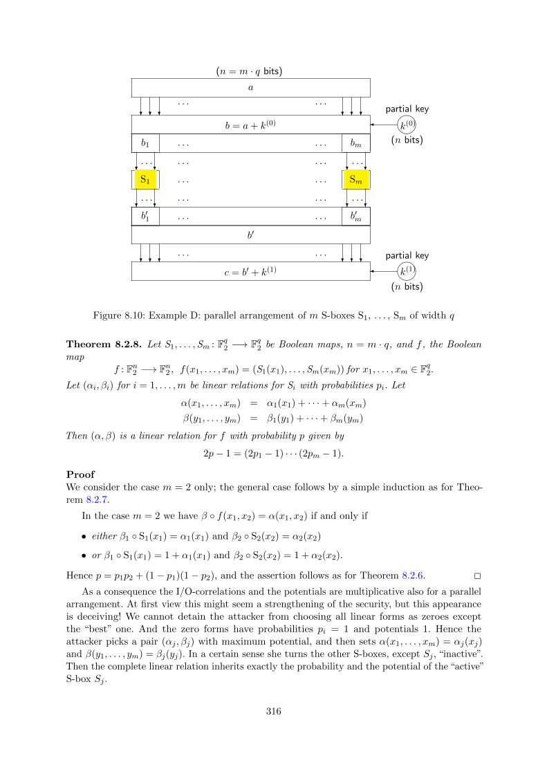
(n = m · q bits)
a
???. . . . . .
??? partial key
k(0)
(n bits)�����b = a+ k(0)
b1 . . . . . . bm
?. . .?
. . . . . .?. . .?
S1
?. . .?
. . . . . .
. . . . . .
Sm
?. . .?
b′1 . . . . . . b′m
b′
c = b′ + k(1)
partial key
k(1)
(n bits)�����
???. . . . . .
???
Figure 8.10: Example D: parallel arrangement of m S-boxes S1, . . . , Sm of width q
Theorem 8.2.8. Let S1, . . . ,Sm : Fq2 −→ Fq2 be Boolean maps, n = m · q, and f , the Booleanmap
f : Fn2 −→ Fn2 , f(x1, . . . , xm) = (S1(x1), . . . ,Sm(xm)) for x1, . . . , xm ∈ Fq2.Let (αi, βi) for i = 1, . . . ,m be linear relations for Si with probabilities pi. Let
α(x1, . . . , xm) = α1(x1) + · · ·+ αm(xm)
β(y1, . . . , ym) = β1(y1) + · · ·+ βm(ym)
Then (α, β) is a linear relation for f with probability p given by
2p− 1 = (2p1 − 1) · · · (2pm − 1).
ProofWe consider the case m = 2 only; the general case follows by a simple induction as for Theo-rem 8.2.7.
In the case m = 2 we have β ◦ f(x1, x2) = α(x1, x2) if and only if
• either β1 ◦ S1(x1) = α1(x1) and β2 ◦ S2(x2) = α2(x2)
• or β1 ◦ S1(x1) = 1 + α1(x1) and β2 ◦ S2(x2) = 1 + α2(x2).
Hence p = p1p2 + (1− p1)(1− p2), and the assertion follows as for Theorem 8.2.6. 2
As a consequence the I/O-correlations and the potentials are multiplicative also for a parallelarrangement. At first view this might seem a strengthening of the security, but this appearanceis deceiving! We cannot detain the attacker from choosing all linear forms as zeroes exceptthe “best” one. And the zero forms have probabilities pi = 1 and potentials 1. Hence theattacker picks a pair (αj , βj) with maximum potential, and then sets α(x1, . . . , xm) = αj(xj)and β(y1, . . . , ym) = βj(yj). In a certain sense she turns the other S-boxes, except Sj , “inactive”.Then the complete linear relation inherits exactly the probability and the potential of the “active”S-box Sj .
316

a a3 c c0 + c1 + c3 estimate
00011110 1 00000010 0 100101100 0 00111111 1 110110010 1 01011101 0 110110100 1 01010000 0 110110101 1 01010111 0 1
Table 8.18: Calculations for example D (parallel arrangement of m S-boxes)
Example
Once again we consider a concrete example with m = 2 and q = 4, hence n = 8. As S-boxes wetake the ones from Lucifer, S0 at the left, and S1 at the right, see Figure 8.10. For the leftS-box S0 we take the linear relation with α = 0001 and β = 1101, that we know has probabilityp1 = 7
8 . For the right S-Box S1 we take the relation (0, 0) (where both linear forms are 0). Sincealways 0 = 0 its probability is 1. The combined linear relation for f = (S0,S1) then also hasprobability p = 7
8 and potential λ = 916 by Theorem 8.2.8, and we know that linear cryptanalysis
with N = 5 pairs of plaintext and ciphertext has (more than) 95% success probability. Wedecompose all relevant bitblocks into bits:
plaintext: a = (a0, . . . , a7) ∈ F82,
ciphertext: c = (c0, . . . , c7) ∈ F82,
key: k = (k0, . . . , k15) ∈ F162 where (k0, . . . , k7) serves as “initial key” (corresponding to k(0) in
Figure 8.10), and (k8, . . . , k15) as “final key” (corresponding to k(1)).
Then α(a) = a3, β(c) = c0 +c1 +c3, and κ(k) = α(k0, . . . , k7)+β(k8, . . . , k15) = k3 +k8 +k9 +k11.Hence the target relation is
k3 + k8 + k9 + k11 = a3 + c0 + c1 + c3.
We use the key k = 1001011000101110 whose relevant bit is k3 +k8 +k9 +k11 = 1, and generatefive random pairs of plaintext and ciphertext82, see Table 8.18. We see that for this exampleMatsui’s algorithm guesses the relevant key bit correctly with no dissentient.
8.2.12 Mini-Lucifer
As a slightly more complex example we define a toy cipher “Mini-Lucifer” that employs theS-boxes and a permutation of the true Lucifer. Here is the construction, see Figure 8.11:
• Before and after each round map we add a partial key. We use two keys k(0) and k(1)
in alternating order. They consist of the first or last 8 bits of the 16 bit master key. Inparticular for r ≥ 3 the round keys are not independent.
• The round function consists of a parallel arrangement of the two S-boxes, as in the exampleof Section 8.2.11, followed by the permutation P.
82We simulate an attacker who knows five pairs of plaintexts and corresponding ciphertexts by generating (arbitrarilyat random) and using these five pairs. Our odds of correctly determining the wanted key bit are very high.
317
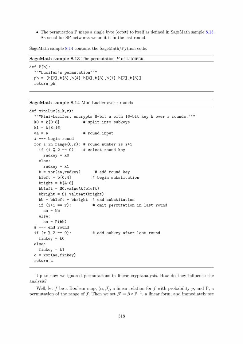
• The permutation P maps a single byte (octet) to itself as defined in SageMath sample 8.13.As usual for SP-networks we omit it in the last round.
SageMath sample 8.14 contains the SageMath/Python code.
SageMath sample 8.13 The permutation P of Lucifer
def P(b):
"""Lucifer’s permutation"""
pb = [b[2],b[5],b[4],b[0],b[3],b[1],b[7],b[6]]
return pb
SageMath sample 8.14 Mini-Lucifer over r rounds
def miniLuc(a,k,r):
"""Mini-Lucifer, encrypts 8-bit a with 16-bit key k over r rounds."""
k0 = k[0:8] # split into subkeys
k1 = k[8:16]
aa = a # round input
# --- begin round
for i in range(0,r): # round number is i+1
if (i % 2 == 0): # select round key
rndkey = k0
else:
rndkey = k1
b = xor(aa,rndkey) # add round key
bleft = b[0:4] # begin substitution
bright = b[4:8]
bbleft = S0.valueAt(bleft)
bbright = S1.valueAt(bright)
bb = bbleft + bbright # end substitution
if (i+1 == r): # omit permutation in last round
aa = bb
else:
aa = P(bb)
# --- end round
if (r % 2 == 0): # add subkey after last round
finkey = k0
else:
finkey = k1
c = xor(aa,finkey)
return c
Up to now we ignored permutations in linear cryptanalysis. How do they influence theanalysis?
Well, let f be a Boolean map, (α, β), a linear relation for f with probability p, and P, apermutation of the range of f . Then we set β′ = β ◦ P−1, a linear form, and immediately see
318

a
?⊕?
round key
k(i) = k(0) or k(1)�
b = a+ k(i)
bli bre
?S0n?
?S1n?
b′li b′re
b′
?Pn . . . except in the last round
?
a′
-
?⊕?
c = a′ + k(r)
k(r) = k(0) or k(1)�
Figure 8.11: Mini-Lucifer over r rounds
319

a
?
b = a+ k(0)
?S0 ?
S1
b′
?P
a′
?
a′ + k(1)
?S0 ?
S1
b′′
?
c = b′′ + k(0)
a0, a1, a2, a3, a4, a5, a6, a7
b0 = a0 + k0, . . . , b7 = a7 + k7
1nb′0 + b′1 + b′3p1≈ a3 + k3
a′0 = b′2, a′1 = b′5, a
′2 = b′4, a
′3 = b′0
a′4 = b′3, a′5 = b′1, a
′6 = b′7, a
′7 = b′6
2na′3 + a′4 + a′5p1≈ a3 + k3
3nb′′0 + b′′1 + b′′3 + b′′5 + b′′6p2≈
a′3 + a′4 + a′5 + k11 + k12 + k13
4nc0 + c1 + c3 + c5 + c6p≈
a3 + k0 + k1 + k5 + k6 + k11 + k12 + k13
Figure 8.12: Mini-Lucifer with 2 rounds
that (α, β′) is a linear relation for P ◦ f with the same probability p:
p =1
2n·#{x ∈ Fn2 | β(f(x)) = α(x)}
=1
2n·#{x ∈ Fn2 | (β ◦ P−1)(P ◦ f(x)) = α(x)}.
The assignment β 7→ β′ simply permutes the linear forms β. In other words: appending apermutation to f permutes the columns of the approximation table, of the correlation matrix,and of the linear profile83.
Inserting a permutation into the round function of an SP-network affects linearcryptanalysis in a marginal way only.
We’ll verify this assertion for a concrete example, and see how “marginal” the effect really is.
Example
The concrete example is specified in Figure 8.12. The relation 1, namely
β(b′)p1≈ α(a+ k(0)), or explicitly b′0 + b′1 + b′3
p1≈ a3 + k3,
holds with probability p1 = 78 between α = 0001 and β = 1101. The permutation P transforms
it to the relation 2, namely
β ◦ P−1(a′)p1≈ α(a+ k(0)) = α(a) + α(k(0)), or explicitly a′3 + a′4 + a′5
p1≈ a3 + k3.
But P also distributes the bits from the left-hand side of the relation over the two S-boxes of thenext round. So the cryptanalytic trick of letting only one S-box per round become active worksonly for the first round.
83By the way the same holds if we replace the permutation by a more general bijective linear map.
320

Inserting a permutation into the round function of an SP-network has the effect thatlinear cryptanalysis has to deal with more than one parallel S-box becoming active inlater rounds.
We’ll soon see in the example that this effect reduces the potential. The relevant bits a′3, a′4, a
′5,
or, after adding the key, a′3 + k11, a′4 + k12, a
′5 + k13, split as input to the left S-box S0 of the
second round (namely a′3 + k11), and to the right one, S1 (namely a′4 + k12 and a′5 + k13).
On the left-hand side, for S0, the linear form for the input is β′1 = 0001 = 1, on the right-handside, for S1, we have β′2 = 1100 = 12. From the linear profile of S0 we see that the maximumpossible potential for β′1 is λ′2 = 9
16 with p′2 = 78 , assumed for γ1 = 13 = 1101.
For β′2 the maximum potential is λ′′2 = 14 . Having two choices we choose γ2 = 6 = 0110 with
probability p′′2 = 34 . The combined linear relation with β′(x) = β′1(x0, . . . , x3) + β′2(x4, . . . , x7)
and, on the output side, γ(y) = γ1(y0, . . . , y3) + γ2(y4, . . . , y7) has I/O-correlation
2p2 − 1 = (2p′2 − 1)(2p′′2 − 1) =3
8
by Theorem 8.2.8, hence p2 = 1116 , λ2 = 9
64 .
The relation between β′(a′ + k(1)) and γ(b′′), namely
γ(b′′)p2≈ β′(a′ + k(1)) = β′(a′) + β′(k(1)),
is labelled by 3 and written in explicit form in Figure 8.12. Combining 2 and 3 (and cancellingk3) yields the relation
γ(c) + γ(k(0)) = γ(c+ k(0)) = γ(b′′)p≈ α(a) + α(k(0)) + β′(k(1)),
given explicitly and labelled by 4 in the figure. Its probability p is given by Theorem 8.2.7 sincethe two round keys are independent. We get
2p− 1 = (2p1 − 1)(2p2 − 1) =3
4· 3
8=
9
32,
whence p = 4164 . The corresponding potential is λ = 81
1024 .
The number N of needed plaintexts for a 95% success probability follows from the approxi-mation in Table 8.11:
N =3
λ=
1024
27≈ 38.
Note that there are only 256 possible plaintexts at all.
In the example the success probability derived from the product of the I/O-correlations (orof the potentials) of all active S-boxes. We had luck since in this example the involved partialkeys were independent. In the general case this is not granted. Nevertheless the cryptanalystrelies on the empirical evidence and ignores the dependencies, trusting the rule of thumb:
The success probability of linear cryptanalysis is (approximately) determined by themultiplicativity of the I/O-correlations (or of the potentials) of all the active S-boxesalong the considered path (including all of its ramifications).
The restriction in this rule of thumb concerns the success probability of linear cryptanalysis butnot the course of action. The cryptanalyst is right if and only if she succeeds, no matter whetherher method had an exact mathematical foundation for all details.
321

Now we obtained a single bit. So what?
Of course we may find more relations, and detect more key bits. However we have to dealwith smaller and smaller potentials, and face an increasing danger of hitting a case where theprobability for the concrete (target) key lies on the “wrong” side of 1
2 . Moreover we run intoa multiple test situation reusing the same known plaintexts several times. This enforces anunpleasant adjustment of the success probabilities.
Systematic Search for Linear Relations
The search for useful linear relations over several rounds has no general elegant solution. Thepublished examples often use linear paths that more or less appear from nowhere, and it is notevident that they are the best ones.
Let n be the block length of the cipher, and r, the number of rounds. Then for each round thechoice is between 2n linear formes, making a total of 2n(r+1) choices. This number also specifiesthe cost of determining the best relation by complete search. There are some simplifications thathowever don’t reduce the order of magnitude of the cost:
• In the first round consider only linear forms that activate only one S-box.
• Then choose the next linear form such that it activates the least possible number of S-boxesof the next round (with high, but not necessarily maximum potential).
• If one of the relations in a linear path has probability 12 , or I/O-correlation 0, then the
total I/O-correlation is 0 by multiplicativity, and this path may be neglected. The same istrue componentwise if the linear forms split among the S-boxes of the respective round.However this negligence could introduce errors since we deal with average probabilities notknowing the key-dependent ones.
For our 2-round example with Mini-Lucifer the systematic search is feasible by pencil andpaper or by a SageMath or Python script. Our example has the following characteristics:
• α = (α1, α2)84 with α1 = 1 = 0001 and α2 = 0 = 0000
• β = (β1, β2) with β1 = 13 = 1101 and β2 = 0 = 0000
• β′ = (β′1, β′2) with β′1 = 1 = 0001, β′2 = 12 = 1100
• γ = (γ1, γ2) with γ1 = 13 = 1101, γ2 = 6 = 0110
• τ1 = 34 , τ ′2 = 3
4 , τ ′′2 = 12 , τ2 = 3
8 , τ = 932 , p = 41
64 = 0, 640625
• c0 + c1 + c3 + c5 + c6p≈ a3 + k0 + k1 + k5 + k6 + k11 + k12 + k13
An alternative choice of γ2 is γ2 = 14 = 1110; this yields a linear path with the characteristics
• α = (1, 0), β = (13, 0), β′ = (1, 12), γ = (13, 14)
– τ = − 932 , p = 23
64 = 0, 359375
– c0 + c1 + c3 + c4 + c5 + c6p≈ a3 + k0 + k1 + k4 + k5 + k6 + k11 + k12 + k13
84α1 was formerly denoted α. Now for uniformity we make both components of all linear forms explicit and indexthem by 1 and 2.
322
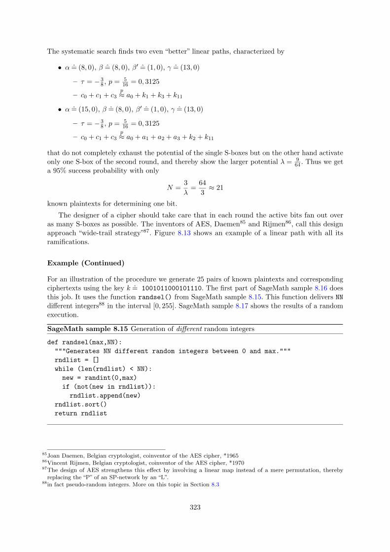
The systematic search finds two even “better” linear paths, characterized by
• α = (8, 0), β = (8, 0), β′ = (1, 0), γ = (13, 0)
– τ = −38 , p = 5
16 = 0, 3125
– c0 + c1 + c3p≈ a0 + k1 + k3 + k11
• α = (15, 0), β = (8, 0), β′ = (1, 0), γ = (13, 0)
– τ = −38 , p = 5
16 = 0, 3125
– c0 + c1 + c3p≈ a0 + a1 + a2 + a3 + k2 + k11
that do not completely exhaust the potential of the single S-boxes but on the other hand activateonly one S-box of the second round, and thereby show the larger potential λ = 9
64 . Thus we geta 95% success probability with only
N =3
λ=
64
3≈ 21
known plaintexts for determining one bit.
The designer of a cipher should take care that in each round the active bits fan out overas many S-boxes as possible. The inventors of AES, Daemen85 and Rijmen86, call this designapproach “wide-trail strategy”87. Figure 8.13 shows an example of a linear path with all itsramifications.
Example (Continued)
For an illustration of the procedure we generate 25 pairs of known plaintexts and correspondingciphertexts using the key k = 1001011000101110. The first part of SageMath sample 8.16 doesthis job. It uses the function randsel() from SageMath sample 8.15. This function delivers NN
different integers88 in the interval [0, 255]. SageMath sample 8.17 shows the results of a randomexecution.
SageMath sample 8.15 Generation of different random integers
def randsel(max,NN):
"""Generates NN different random integers between 0 and max."""
rndlist = []
while (len(rndlist) < NN):
new = randint(0,max)
if (not(new in rndlist)):
rndlist.append(new)
rndlist.sort()
return rndlist
85Joan Daemen, Belgian cryptologist, coinventor of the AES cipher, *196586Vincent Rijmen, Belgian cryptologist, coinventor of the AES cipher, *197087The design of AES strengthens this effect by involving a linear map instead of a mere permutation, thereby
replacing the “P” of an SP-network by an “L”.88in fact pseudo-random integers. More on this topic in Section 8.3
323

SageMath sample 8.16 Linear cryptanalysis of Mini-Lucifer over 2 roundssage: key = str2bbl("1001011000101110")
sage: bit = [0,0,0,0]
sage: bit[0] = (key[0]+key[1]+key[5]+key[6]+key[11]+key[12]+key[13]) % 2
sage: bit[1] = (key[0]+key[1]+key[4]+key[5]+key[6]+key[11]+key[12]+key[13])%2
sage: bit[2] = (key[1]+key[3]+key[11]) % 2
sage: bit[3] = (key[2]+key[11]) % 2
sage: NN = 25
sage: plist = randsel(255,NN)
sage: klist = [[], [], [], []]
sage: for i in range (0,NN):
....: plain = int2bbl(plist[i],8)
....: ciph = miniLuc(plain,key,2)
....: print("pc pair nr", i+1, "is", plain, ciph)
....: kbit = (plain[3]+ciph[0]+ciph[1]+ciph[3]+ciph[5]+ciph[6]) % 2
....: klist[0].append(kbit)
....: kbit = (1+plain[3]+ciph[0]+ciph[1]+ciph[3]+ciph[4]+ciph[5]+ciph[6])%2
....: klist[1].append(kbit)
....: kbit = (1+plain[0]+ciph[0]+ciph[1]+ciph[3]) % 2
....: klist[2].append(kbit)
....: kbit=(1+plain[0]+plain[1]+plain[2]+plain[3]+ciph[0]+ciph[1]+ciph[3])%2
....: klist[3].append(kbit)
[...]
sage: for j in range(0,4):
....: sum = 0
....: for jj in range(0,NN):
....: sum += klist[j][jj]
....: if (bit[j] == 0):
....: sum = NN - sum
....: print("True bit:", bit[j], klist[j])
....: print(" Relation", j+1, ":", sum, "of", NN ,"guesses are correct.")
[...]
The target key bits (that we know in cheat mode) are bit[j] for j = 0, 1, 2, 3. We use all fourgood relations at the same time without fearing the possible reduction of the success probability.All of these relations assert the probable equality of the bits bit[j] and the sums of plain andcipher bits in the rows kbit. For the last three of these sums we have to take the complementarybits since the corresponding I/O-correlations are negative (the probabilities are < 1
2). This isdone by adding the bit 1.
SageMath sample 8.18 shows the result of the analysis. As we see our guess is correct for allfour bits89.
89We didn’t use the function Matsui_Test() in order to gain some insight into the intermediate results.
324

SageMath sample 8.17 25 random pairs of plaintexts and ciphertexts from Mini-Lucifer over2 roundspc pair nr 1 is [0,0,0,0,1,1,1,1] [0,0,0,0,1,0,1,0]
pc pair nr 2 is [0,0,0,1,0,0,0,1] [1,1,0,0,1,1,1,0]
pc pair nr 3 is [0,0,0,1,0,1,1,0] [1,1,0,0,1,0,0,1]
pc pair nr 4 is [0,0,1,1,1,1,0,1] [1,0,1,1,0,0,1,0]
pc pair nr 5 is [0,1,0,0,0,0,0,0] [1,1,1,0,0,1,1,1]
pc pair nr 6 is [0,1,0,0,1,0,0,0] [0,1,0,1,0,1,1,1]
pc pair nr 7 is [0,1,0,0,1,1,0,0] [1,1,1,0,1,0,1,0]
pc pair nr 8 is [0,1,0,0,1,1,0,1] [0,1,0,1,1,1,0,0]
pc pair nr 9 is [0,1,0,0,1,1,1,1] [0,1,1,1,1,0,1,0]
pc pair nr 10 is [0,1,1,0,0,1,1,1] [0,0,1,1,0,0,1,1]
pc pair nr 11 is [1,0,0,0,0,0,1,1] [1,1,1,1,0,1,0,0]
pc pair nr 12 is [1,0,0,1,0,0,1,1] [0,1,1,0,1,0,1,1]
pc pair nr 13 is [1,0,0,1,1,0,0,0] [0,1,1,0,0,1,1,1]
pc pair nr 14 is [1,0,1,0,1,0,1,1] [1,1,0,1,1,0,0,1]
pc pair nr 15 is [1,0,1,1,0,0,0,1] [1,1,0,0,1,0,0,0]
pc pair nr 16 is [1,0,1,1,0,0,1,0] [1,0,1,0,0,1,0,0]
pc pair nr 17 is [1,0,1,1,0,1,1,0] [1,1,0,0,0,1,0,0]
pc pair nr 18 is [1,0,1,1,1,0,0,1] [1,1,0,0,0,0,0,1]
pc pair nr 19 is [1,0,1,1,1,1,0,1] [1,0,1,1,1,1,1,1]
pc pair nr 20 is [1,1,0,0,0,1,0,0] [0,1,0,0,1,1,1,1]
pc pair nr 21 is [1,1,0,0,0,1,1,1] [0,0,1,1,1,1,1,1]
pc pair nr 22 is [1,1,0,1,1,1,1,1] [1,1,0,1,1,0,1,0]
pc pair nr 23 is [1,1,1,0,0,0,0,0] [1,1,1,0,1,1,1,0]
pc pair nr 24 is [1,1,1,0,0,1,0,0] [0,1,1,1,0,0,1,1]
pc pair nr 25 is [1,1,1,1,0,1,0,1] [1,1,1,1,0,1,0,1]
SageMath sample 8.18 Linear cryptanalysis of Mini-Lucifer over 2 rounds
True bit: 1 [1,1,1,0,0,0,1,1,1,0,0,1,0,1,1,1,0,1,1,1,1,1,0,1,1]
Relation 1 : 17 of 25 guesses are correct.
True bit: 1 [1,1,1,1,1,1,1,1,1,1,1,1,1,1,1,0,1,0,1,1,1,1,0,0,0]
Relation 2 : 20 of 25 guesses are correct.
True bit: 1 [1,1,1,1,1,1,1,1,1,0,1,1,1,1,0,1,0,0,0,1,1,1,0,0,1]
Relation 3 : 18 of 25 guesses are correct.
True bit: 0 [1,0,0,1,0,0,0,0,0,0,1,0,0,0,0,1,0,0,0,0,0,1,0,0,0]
Relation 4 : 20 of 25 guesses are correct.
325

As a consequence of our analysis we get a system of four linear equations for the 16 unknownkey bits:
1 = k0 + k1 + k5 + k6 + k11 + k12 + k13
1 = k0 + k1 + k4 + k5 + k6 + k11 + k12 + k13
1 = k1 + k3 + k11
0 = k2 + k11
that allow us to reduce the number of keys for an exhaustion from 216 = 65536 to 212 = 4096.Note the immediate simplifications of the system: k11 = k2 from the last equation, and k4 = 0from the first two.
As a cross-check we run some more simulations. The next four yield
• 15, 16, 19, 16
• 15, 16, 13, 17
• 15, 20, 19, 17
• 19, 19, 20, 18
correct guesses, and so on. Only run number 10 produced a wrong bit (the second one):
• 17, 12, 14, 17
then again run number 25. Thus empirical evidence suggests a success probability of at least90% in this scenario.
Analysis over Four Rounds
Now let’s explore how an increasing number of rounds impedes linear cryptanalysis.
Consider the toy cipher Mini-Lucifer over four rounds. Searching an optimal linear path overfour rounds is somewhat expensive, so we content ourselves with extending the best example fromthe two round case, the third one, over two additional rounds. Slightly adapting the notation weget:
• for the first round β0 = α = (8, 0) and β1 = (8, 0) (the “old” β) with τ1 = −12 ,
• for the second round (applying the permutation P to β1) β′1 = (1, 0) and β2 = (13, 0) (the
“old” γ) with τ2 = 34 ,
• for the third round β′2 = (1, 12) and β3 = (13, 6) with τ3 = 38 ,
• for the fourth round β′3 = (5, 13) and β = β4 = (3, 12) (the “new” β) with τ4 = −14 .
Figure 8.13 shows this linear path with its ramifications.
The repeated round keys we used are not independent. Therefore multiplicativity of I/O-correlations is justified by the rule of thumb only yielding an approximate value for the I/O-correlation of the linear relation (α, β) over all of the four rounds:
τ ≈ 1
2· 3
4· 3
8· 1
4=
9
256≈ 0, 035.
326

1 0 0 0 0 0 0 0 α = β0 = (8, 0)
?St@@R
��
t1 0 0 0 0 0 0 0 β1 = (8, 0)
?P
@@@@R
0 0 0 1 0 0 0 0 β′1 = (1, 0)
?S
��
���� @@R
t t1 1 0 1 0 0 0 0 β2 = (13, 0)
?P
@@@@R
HHHHH
HHj
@@@@R
0 0 0 1 1 1 0 0 β′2 = (1, 12)
?St��
��@@R��
t@@RBBN�� BBN
1 1 0 1 0 1 1 0 β3 = (13, 6)
?P
@@@@R
HHHH
HHHj
@@@@R
����
����
BBBBN
0 1 0 1 1 1 0 1 β′3 = (5, 13)
?StBBN ��
BBN@@R
t@@RBBN ������
0 0 1 1 1 1 0 0 β = β4 = (3, 12)
Figure 8.13: A linear path with ramifications (“trail”). For S the linear form in the range ischosen (for high potential), indicated by a red dot. For P the linear form in the range results byapplying the permutation.
The other characteristics are
p ≈ 265
512≈ 0, 518, λ ≈ 81
65536≈ 0, 0012, N ≈ 65536
27≈ 2427,
the last one being the number of needed known plaintexts for a 95% success probability.
Comparing this with the cost of exhaustion over all 65536 possible keys we seem to havegained an advantage. However there are only 256 different possible plaintexts all together. Solinear cryptanalysis completely lost its sense by the increased number of rounds.
8.2.13 Outlook
As we saw linear cryptanalysis provides some evidence for the security of a cipher, in particularfor choosing the number of rounds. But only some parts of the theory have a mathematicallysatisfying basis. Most existing publications only give ad-hoc analyses of concrete ciphers. Forexample Matsui showed how for DES 243 known plaintexts reveal 14 key bits with high certainty,
327

ciphertext block?
...
?⊕?
f roundfunctionl?
...
?⊕?
plaintext block
keyblock
-partial key k(i−1)
-partial key k(r)
i-th round
Figure 8.14: Structure of AES in the large
reducing the exhaustion to the remaining 42 = 56− 14 key bits, a feasible task (at least if theanalyst gets that many plaintexts).
The treatment of linear cryptanalysis serves as an example of similar analyses. Differentialcryptanalysis as well as generalized and mixed variants follow similar lines of thought. For moreinformation see the book [Sti06] that also explicitly specifies the most important ciphers DESand AES.
AES
Figures 8.14 and 8.15 show the design of AES90 in the large and show the realization of thedesign principles derived in the former subsections.
• The block length is n = 128, the key length, l = 128, 192, or 256, the number of rounds,r = 10, 12, or 14.
• At the beginning of each round and after the last round a partial key is added to thecurrent bitblock, as in examples A, B, C, Figures 8.5, 8.8, 8.9. The complete algorithminvolves r + 1 partial keys.
• The 128-bit “partial keys” k(i) are not partial keys in the proper sense but extractedfrom the master key k by a somewhat involved algorithm (“key schedule”). They are notindependent.
• Each round starts by splitting the current 128-bit block into 16 parts each consistingof 8 bits. Each of this parts is fed into the same S-box S: F8
2 −→ F82. This S-box has a
mathematically quite elegant description that however assumes some advanced knowledge
90in CrypTool 2 found under “modern” / “symmetric”.
328

???. . . . . .
???
decomposition into 8-bit blocks
?. . .?
. . . . . .?. . .?
@@R?��
. . . permutation / linear map . . . @@R?��
???. . . . . .
???
?. . .?
. . . . . .parallel applications of the S-box
. . . . . .?. . .?
S S
Figure 8.15: The round function f of AES
of abstract algebra, hence is omitted here. The linear potential of the S-box is 164 . The
method linProf() of the class boolMap, SageMath sample 8.47, explicitly confirms this,but there is also a “deep” mathematical reason91.
• The “diffusion step” consists of a permutation followed by a linear map. This step is slightlymore complex than for a pure SP-network as in Figure 8.2.
A final remark on the key schedule: If the round keys, k(i) in our notation, are not simplypartial keys but extracted by a more complex procedure, then the true master key is concealed.The cryptanalyst however attacks the “effective” key, consisting of the round keys k(i). Thissuffices to break the cipher. Nevertheless a complex key schedule makes a cipher more securefor it detains the attacker from explicitly utilizing the dependence of the various round keys, inparticular if they consist of overlapping blocks of master key bits.
91that as a mathematical miracle involves counting the points of elliptic curves over finite fields of characteristic 2
329

8.3 Bitstream Ciphers
A bitstream cipher sequentially encrypts each single bit of a bitstring by an individual rule.The two possibilities are: leave the bit unchanged, or negate it. Leaving the bit unchanged isequivalent with (binary) adding 0, negating the bit is equivalent with adding 1. Thus everybitstream cipher may be interpreted as an XOR encryption92 in the sense of the followingsubsection 8.3.1. We distinguish between
synchronous bitstream ciphers where the key stream is generated independently of theplaintext,
asynchronous bitstream ciphers where the key stream depends on the plaintext or othercontext parameters.
In this chapter we only treat synchronous bitstream ciphers. We also exclude stream ciphersover other character sets than the bits 0, 1.
8.3.1 XOR Encryption
plaintext bits
a1a2a3 . . .
k1k2k3 . . .
key bits
c1c2c3 . . .
ciphertext bits
ci = ai + ki
PPPPPPq
������1&%'$XOR -
Figure 8.16: The principle of XOR encryption
The basic method of bitstream encryption is simply denoted by XOR. It interprets plaintexts93
as sequences of bits. Also the key is a bit sequence, called key stream. The encryption algorithmadds the current bit of the plaintext and the current bit of the key stream by XOR. Figure 8.16illustrates the algorithm94, Figure 8.17 shows an example.
a: 01000100011101 ...
k: 10010110100101 ...
------------------
c: 11010010111000 ...
Figure 8.17: Example of XOR encryption
92the key being the “difference” between ciphertext and plaintext as in Figure 8.1993The SageMath method ascii_to_bin() from the module sage.crypto.util converts“ordinary” texts to bitstrings.
The inverse method is bin_to_ascii(). However these bitstrings belong to the class StringMonoidElement, soneed a proper context. Therefore in SageMath sample 8.38 we define functions txt2bbl that transforms ASCIItexts to bitblocks, and bbl2str that transforms bitblocks to bitstrings.
94In CrypTool 2 under “classic”/ “XOR”, in Appendix 8.4.3 as xor, see SageMath sample 8.39.
330

In the twenties of the 20th century XOR ciphers were invented to encrypt teleprinter messages.These messages were written on five-hole punched tapes as in Figure 8.18. Another punched tapeprovided the key stream. Vernam95 filed his U. S. patent in 1918. He used a key tape whose endswere glued together, resulting in a periodic key stream. Mauborgne96 immediately recognizedthat a nonperiodic key is obligatory for security.
�@�@
@�@�
tdtdtdddtdttttddddtdtttttttddtdddttttdtttdtdtdddtdttddt
Figure 8.18: Punched tape—each column represents a five-bit character
In its strongest form, the one-time pad (OTP), XOR encryption is an example for perfectsecurity in the sense of Shannon. As algorithm A5 or E0 XOR helps to secure mobile phones orthe Bluetooth protocol for wireless data transmission. As RC4 it is part of the SSL protocol that(sometimes) encrypts client-server communication in the World Wide Web, and of the PKZIPcompression software. There are many other current applications, not all of them fulfilling theexpected security requirements.
The scope of XOR encryption ranges from simple ciphers that are trivially broken tounbreakable ciphers.
Advantages of XOR ciphers:
• Encryption and decryption are done by the same algorithm: Since ci = ai + ki alsoai = ci + ki. Thus decryption also consists of adding key stream and ciphertext(elementwise binary).
• The method is extremely simple to understand and to implement
• . . . and very fast—provided that the key stream is available. For high transfer ratesone may precompute the key stream at both ends of the line.
• If the key stream is properly chosen the security is high.
Disadvantages of XOR ciphers:
• XOR ciphers are vulnerable for known plaintext attacks: each correctly guessedplaintext bit reveals a key bit.
• If the attacker knows a piece of plaintext she also knows the corresponding piece ofthe key stream, and then is able to exchange this plaintext at will. For example shemight replace “I love you” by “I hate you”, or replace an amout of $1000 by $9999. Inother words the integrity of the message is poorly protected97.
• XOR ciphers provide no diffusion in the sense of Shannon’s criteria since each plaintextbit affects the one corresponding plaintext bit only98.
95Gilbert Vernam, U. S. American engineer, April 3, 1890 – February 7, 196096Joseph Mauborgne, Major General in the U. S. Army, February 26, 1881 – July 7, 197197To protect message integrity the sender has to implement an additional procedure.98Block ciphers in the opposite were designed for using diffusion.
331

• Each reuse of a part of the key sequence (also in form of a periodic repetition) opensthe door for an attack. The historical successes in breaking stream ciphers almostalways used this effect, for example the attacks on encrypted teleprinters in WorldWar II, or the project Venona during the Cold War.
A remark on the first item, the vulnerability for attacks with known plaintext: The commonISO character set for texts has a systematic weakness. The 8-bit codes99 of the lower-case lettersa..z all start with 011, of the upper-case letters A..Z, with 010. A supposed sequence of sixlower-case letters (no matter which) reveals 6 · 3 = 18 key bits.
In other words: We cannot prevent the attacker from getting or guessing a good portionof the plaintext. Thus the security against an attack with known plaintext is a fundamentalrequirement for an XOR cipher, even more than for any other cryptographic procedure.
8.3.2 Generating the Key Stream
The main naive methods for generating the key stream are:
• periodic bit sequence,
• running-text,
• “true” random sequence.
A better method uses a
• pseudo-random sequence
and leads to really useful procedures. The essential criterion is the quality of the pseudo-randomgenerator.
Periodic Bit Sequence
Example We generate a key stream of period 8 by repeating k = 10010110. We representletters by bytes in the ISO character set.
C | o | m | e | | a |
a: 01000011|01101111|01101101|01100101|00100000|01100001|
k: 10010110|10010110|10010110|10010110|10010110|10010110|
-------- -------- -------- -------- -------- --------
c: 11010101|11111001|11111011|11110011|10110110|11110111|
t | | n | i | n | e
01110100|00100000|01101110|01101001|01101110|01100101
10010110|10010110|10010110|10010110|10010110|10010110
-------- -------- -------- -------- -------- --------
11100010|10110110|11111000|11111111|11111000|11110011
99By the way the appearance of many zeroes in the leading bits of the bytes is an important identifying feature oftexts in many european languages.
332

This encryption is easily done by hand, or by SageMath sample 8.19.
If we re-encode the ciphertext bytes in the ISO-8859-1 character set the cryptogram lookslike this:
O u u o ¶ ÷ a ¶ ø y ø o
This might bedazzle laypersons. An expert immediately notes that all characters are from theupper half of the possible 256 bytes. This observation suggests that the plaintext is in naturallanguage, encrypted with a key whose leading bit is 1. If the attacker guesses that the conspicuouscharacter ¶ = 10110110 corresponds to the space character 00100000, she derives the key asthe difference 10010110. This breaks the cryptogram.
Known or probable plaintext easily breaks periodic XOR encryption.
SageMath sample 8.19 XOR encryption in Python/SageMath
sage: testtext = "Come at nine"
sage: bintext = txt2bbl(testtext)
sage: binstr = bbl2str(bintext); binstr
’010000110110111101101101011001010010000001100001
011101000010000001101110011010010110111001100101’
sage: testkey = [1,0,0,1,0,1,1,0]
sage: keystr = bbl2str(testkey); keystr
’10010110’
sage: cipher = xor(bintext,testkey)
sage: ciphstr = bbl2str(cipher); ciphstr
’110101011111100111111011111100111011011011110111
111000101011011011111000111111111111100011110011’
MS Word and Periodic XOR
The following table (generated ad hoc by simple character counts) shows the frequencies of themost frequent bytes in MS Word files.
byte (hexadecimal) bits frequency
00 00000000 7–70%01 00000001 0.8–17%20 (space) 00100000 0.8–12%65 (e) 01100101 1–10%FF 11111111 1–10%
Note that these frequencies relate to the binary files, heavily depend on the type of the document,and may change with every software version. The variation is large, we often find unexpectedpeaks, and all bytes 00–FF occur. But all this doesn’t matter here since we observe
long chains of 00 bytes.
For an MS Word file that is XOR encrypted with a periodically repeated key the ubiquity ofzeroes suggests an efficient attack: Split the stream of ciphertext bits into blocks corresponding to
333

the length of the period100 and add the blocks pairwise. If one of the plaintext blocks essentiallyconsists of zeroes, then the sum is readable plaintext. Why? Consider the situation
. . . block 1 . . . block 2 . . .
plaintext: . . . a1 . . . as . . . 0 . . . 0 . . .key: . . . k1 . . . ks . . . k1 . . . ks . . .
ciphertext: . . . c1 . . . cs . . . c′1 . . . c′s . . .
where ci = ai + ki and c′i = 0 + ki = ki for i = 1, . . . , s. Thus the key reveals itself in block 2,however the attacker doesn’t recognize this yet. But tentatively paarwise adding all blocks shegets (amongst other things)
ci + c′i = ai + ki + ki = ai for i = 1, . . . , s,
that is, a plaintext block. If she realizes this (for example recognizing typical structures), thenshe sees the key k1, . . . , ks.
Should it happen that the sum of two ciphertext blocks is zero then the ciphertext blocksare equal, and so are the corresponding plaintext blocks. The probability that both of them arezero is high. Thus the key could immediately show through. To summarize:
XOR encryption with a periodic key stream is quite easily broken for messages witha known structure.
This is true also for a large period, say 512 bytes = 4096 bits, in spite of the hyperastronomicallyhuge key space of 24096 different possible keys.
Running-Text Encryption
A classical approach to generating an aperiodic key is taking a data stream, or file, or text,that has at least the length of the plaintext. In classical cryptography this method was calledrunning-text encryption, and the keys were taken from books101 beginning at a certain position.The main method of breaking the cipher was finding or guessing the book. The same weaknessaffects the electronic analog that uses a file, or a CD, or DVD: As soon as the attacker knowsthe source of the key bits the key space is much too small—exhausting a file of several gigabytesis easily done, the costs are linear in the size of the file.
But even when the attacker is unable to guess the source of the key bits ciphertext-onlycryptanalysis is possible: Plaintexts as well as keys contain structures that are not completelyconcealed by binary addition. We won’t discuss this here102 but summarize:
XOR encryption with running-text keys is fairly easily broken.
True Random Sequence
The extreme choice for a key is a true random sequence of bits as key stream. Then the cipheris called (binary) one-time pad (OTP). In particular no part of the key stream must be
100If the length of the period is unknown, determine it by the methods for periodic polyalphabetic substitutions fromclassical cryptanalysis named after Kasiski, Friedman, or Sinkov. Or simply try all possible lengths.
101one of several ways of using a book as cryptographic key that in classical cryptography are denoted as “bookciphers”
102JCrypTool offers an automatic recognition of plaintext and key that uses ciphertext only, see “Analysis”/“Viterbianalysis”.
334

repeated at any time. The notation “pad” comes from the idea of a tear-off calendar—each sheetis destroyed after use. This cipher is unbreakable, or “perfectly secure”. Shannon gave a formalproof of this, see [Sti06].
Without mathematical formalism the argument is as follows: The ciphertext divulges noinformation about the plaintext (except the length). It could result from any plaintext of thesame length: simply take the (binary) difference of ciphertext and alleged plaintext as key.Consider the ciphertext c = a+ k with plaintext a and key k, all represented by bitstreams andadded bit by bit as in Figure 8.16. For an arbitrary different plaintext b the formula c = b+ k′
likewise shows a valid encryption using k′ = b+ c as key.
This property of the OTP could be used in a scenario of forced decryption103 to produce aninnocuous plaintext, as exemplified in Figure 8.19.
If the one-time pad is perfect—why not use it in any case?
• The key management is unwieldy: Key agreement becomes a severe problem since the keyis as long as the plaintext and awkwardly to memorize. Thus the communication partnershave to agree on the key stream prior to transmitting the message, and store it. Agreeingon a key only just in time needs a secure communication channel—but if there was onewhy not use it to transmit the plaintext in clear?
• The key management is inappropriate for mass application or multi-party communicationbecause of its complexity that grows with each additional participant.
• The problem of message integrity requires an extended solution for OTP like for any XORcipher.
There is another, practical, problem when encrypting on a computer: How to get randomsequences? “True random” bits arise from physical events like radioactive decay, or thermal noiseon an optical sensor. The apparently deterministic machine “computer” can also generate truerandom bits, for instance by special chips that produce usable noise. Moreover many events areunpredictable, such as the exact mouse movements of the user, or arriving network packets that,although not completey random, contain random ingredients that may be extracted. On Unixsystems these are provided by /dev/random.
However these random bits, no matter how “true”, are not that useful for encryption by OTP.The problem is on the side of the receiver who cannot reproduce the key. Thus the key streammust be transmitted independently.
There are other, useful, cryptographic applications of “true” random bits: Generating keysfor arbitrary encryption algorithms that are unpredictable for the attacker. Many cryptographicprotocols rely on “nonces” that have no meaning except for being random, for example theinitialization vectors of the block cipher modes of operation, or the “challenge” for strongauthentication (“challenge-response protocol”).
For XOR encryption—as approximation to the OTP—algorithmically generated bit sequencesare much more practicable. But the attacker should have no means to distinguish them fromtrue random sequences. This is the essence of the concept “pseudo-randomness”, and generatingpseudo-random sequences is of fundamental cryptologic relevance.
XOR encryption with a pseudo-random key stream spoils the perfect security ofthe one-time pad. But if the pseudo-random sequence is cryptographically strong(Section 8.3.9) the attacker has no chance to exploit this fact.
103also known as “rubber hose cryptanalysis”
335

Plain bits and text:
01010100 01101000 01101001 01110011 00100000 01101101 This m
01100101 01110011 01110011 01100001 01100111 01100101 essage
00100000 01101001 01110011 00100000 01101000 01100001 is ha
01111010 01100001 01110010 01100100 01101111 01110101 zardou
01110011 00101110 s.
Key bits:
11001000 11010110 00110011 11000000 00111011 10001110
00001000 11101111 01001001 11100101 10111100 10111001
00010010 11000110 01110011 11010111 11000100 01100000
11100110 00010111 01101010 10111011 00010101 11011000
11110000 01000010
Cipher bits:
10011100 10111110 01011010 10110011 00011011 11100011
01101101 10011100 00111010 10000100 11011011 11011100
00110010 10101111 00000000 11110111 10101100 00000001
10011100 01110110 00011000 11011111 01111010 10101101
10000011 01101100
Pseudokey bits:
11001000 11010110 00110011 11000000 00111011 10001110
00001000 11101111 01001001 11100101 10111100 10111001
00010010 11000110 01110011 11010111 11000101 01101111
11110010 00011001 01111011 10101010 00010101 11011000
11110000 01000010
Pseudodecrypted bits and text:
01010100 01101000 01101001 01110011 00100000 01101101 This m
01100101 01110011 01110011 01100001 01100111 01100101 essage
00100000 01101001 01110011 00100000 01101001 01101110 is in
01101110 01101111 01100011 01110101 01101111 01110101 nocuou
01110011 00101110 s.
Figure 8.19: XOR encryption of a hazardous message, and an alleged alternative plaintext
336

8.3.3 Pseudo-Random Generators
Pseudo-random generators mimic true random processes by deterministic algorithms. Usuallysuch an algorithm is called random generator, omitting the prefix “pseudo” if there is no danger ofconfusion. The main difference between a pseudo-random sequence and a true random sequenceis its reproducibility.
Cipher designers hope to approximate the ideal properties of the one-time pad by using apseudo-random bit sequence as key stream treating the short start string as “effective key”. Evenfor random generators of modest quality the resulting ciphertexts are immune against statisticalanalyses. The all-dominant problem is the security against known plaintext attacks.
Thus the critical question for a pseudo-random sequence and for a random generator is:
Given a known chunk (maybe fragmented) of the sequence, is there a way to determinesome more bits of the sequence, be it forwards or backwards?
For “classical” random generators that are popular in statistical applications and simulations theanswer is YES, see Section 8.3.4. But we’ll learn about random generators that—presumably—are cryptographically secure. The cipher designer faces the problem of finding a good trade-offbetween efficiency and security.
The main serious methods of generating pseudo-random bit sequences, or key streams, are:
• (feedback) shift registers (FSR) and combinations thereof, with theoretical foundations inBoolean algebra,
• perfect random generators with theoretical foundations in number theory.
Figure 8.20 shows the schematic functionality of a random generator. It hides an inner statethat changes with each step by a given algorithm. This algorithm is controlled by parameterssome of which are “public”, but some of which are secret and serve as components of the key.The initial state (= start value) is a true random value and likewise secret. With each stepthe random generator outputs a value, depending on its current inner state, until an exteriorintervention stops it.
s s
rs
state
state transition algorithm
secret part (“black box”)
internal parameters (secret)
?
initial state -
external parameters (public)
6
-
output(one element per state)
to be used aspseudo-random sequence
Figure 8.20: (Pseudo-)random generator
Thus the random generator transforms a short, truely random, bit sequence, the initial state,into a long pseudo-random sequence. Cryptologists call this effect “key expansion”.
337

Feedback Shift Registers
Feedback shift registers (FSR) are a classical and popular method of generating pseudo-randomsequences. The method goes back to Golomb104 in 1955, but is often named after Tausworthe whopicked up the idea in a 1965 paper. FSRs are especially convenient for hardware implementation.
An FSR of length l is specified by a Boolean function f: Fl2 −→ F2, the “feedback function”.Figure 8.21 shows the mode of operation. The output consists of the rightmost bit u0, all theother bits are shifted to the right by one position, and the leftmost cell is filled by the bitul = f(ul−1, . . . , u0). Thus the recursive formula
un = f(un−1, . . . , un−l) fur n ≥ l (8.9)
represents the complete sequence. SageMath sample 8.20 defines a general FSR with feedbackfunction f , SageMath sample 8.21 uses it to generate a bit sequence by a concrete samplefeedback function. Table 8.19 illustrates the stepping of the register. Note that the result doesn’tlook convincingly random, and take this as warning that the choice of the parameters needssignificantly more care.
The bits u0, . . . , ul−1 form the start value. The key expansion transforms the short sequenceu = (u0, . . . , ul−1) (the effective key) of length l into a key stream u0, u1, . . . of arbitrary length105.Additionally in this context treating the internal parameters, that is the feedback function for some of its coefficients, as components of the key makes sense. This makes the effective keylength larger than l.
In this respect the realization in hardware differs from a software implementation: Hardwareallows using an adjustable feedback function only by complex additional circuits. Thus in thiscase we usually assume an unchangeable feedback function, and (at least in the long run) wecannot prevent the attacker from figuring it out. In contrast a software implementation allows acomfortable change of the feedback function at any time such that it may serve as part of thekey.
ul−1 . . . . . . u2 u1 u0-
ul
- u0
�� ��f
6 6 66
. . . . . .
- ---
Figure 8.21: A feedback shift register (FSR) during the first iteration step. The Boolean functionf calculates a new bit from the current state of the register. This new bit is slid in from the left.
The Period of a Finite-State Machine
In computer science a feedback shift register is a special case of a finite-state machine. Therefore,the sequence of its states is periodic. Here is why.
104Solomon W. Golomb, U. S. American mathematician and engineer, ∗May 30, 1932105In a cryptographic context the bits u0, u1, . . . form the secret key stream. In other contexts there might be no
need to conceal the output bits, but even then hiding the initial state might make sense, starting the outputsequence at ul.
338

SageMath sample 8.20 A feedback shift register (FSR) in Python/SageMath
def fsr(f,x,n):
"""Generate a feedback shift register sequence.
Parameters: Boolean function f, start vector x,
number n of output bits."""
u = x
outlist = []
for i in range (0,n):
b = f.valueAt(u)
c = u.pop()
u.insert(0,b)
outlist.append(c)
return outlist
SageMath sample 8.21 A (very poor) pseudo-random sequence in Python/SageMath
sage: bits = "1000010111001001"
sage: x = str2bbl(bits)
sage: f = BoolF(x)
sage: start = [0,1,1,1]
sage: bitlist = fsr(f, start, 32)
sage: print(bbl2str(bitlist))
11101010101010101010101010101010
Let M be a finite set of m = #M elements. Imagine M as the collection of all possible statesof a machine. Cosider a map (“transition”)
g : M −→M.
For each element (“initial state”) x0 ∈M define a sequence (xi)i≥0 in M by the recursive formulaxi = g(xi−1) for i ≥ 1. After a preperiod of length µ the sequence runs into a period of length ν,see Figure 8.22, an explanation follows.
Since the set M is finite the states must eventually repeat. Thus there are smallest integersµ ≥ 0 and ν ≥ 1 such that xµ+ν = xµ: To see this simply take µ as the first index such that theelement xµ reappears in the sequence at another position, and µ+ ν as the first index wherethis repetition occurs. Then also (by induction)
xi+ν = g(xi+ν−1) = g(xi−1) = xi for i > µ.
feedback state output
start 0111 −→ 1f(0111) = 1 −→ 1011 −→ 1f(1011) = 0 −→ 0101 −→ 1f(0101) = 1 −→ 1010 −→ 0f(1010) = 0 −→ 0101 from here on periodic
Table 8.19: The stepping of a sample FSR
339
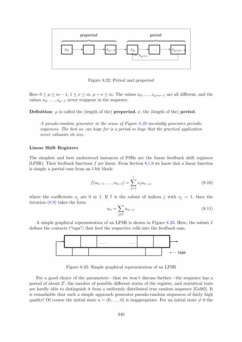
- - - - -x0 . . . xµ−1 xµ= xµ+ν
. . . xµ+ν−1
��6︷ ︸︸ ︷preperiod ︷ ︸︸ ︷period
Figure 8.22: Period and preperiod
Here 0 ≤ µ ≤ m− 1, 1 ≤ ν ≤ m, µ+ ν ≤ m. The values x0, . . . , xµ+ν−1 are all different, and thevalues x0, . . . , xµ−1 never reappear in the sequence.
Definition: µ is called the (length of the) preperiod, ν, the (length of the) period.
A pseudo-random generator in the sense of Figure 8.20 inevitably generates periodicsequences. The best we can hope for is a period so huge that the practical applicationnever exhausts its size.
Linear Shift Registers
The simplest and best understood instances of FSRs are the linear feedback shift registers(LFSR). Their feedback functions f are linear. From Section 8.1.9 we know that a linear functionis simply a partial sum from an l-bit block:
f(un−1, . . . , un−l) =l∑
j=1
sjun−j , (8.10)
where the coefficients sj are 0 or 1. If I is the subset of indices j with sj = 1, then theiteration (8.9) takes the form
un =∑j∈I
un−j . (8.11)
A simple graphical representation of an LFSR is shown in Figure 8.23. Here, the subset Idefines the contacts (“taps”) that feed the respective cells into the feedback sum.
. . . . . .
tapsL99
- -
Figure 8.23: Simple graphical representation of an LFSR
For a good choice of the parameters—that we won’t discuss further—the sequence has aperiod of about 2l, the number of possible different states of the register, and statistical testsare hardly able to distinguish it from a uniformly distributed true random sequence [Gol82]. Itis remarkable that such a simple approach generates pseudo-random sequences of fairly highquality! Of course the initial state u = (0, . . . , 0) is inappropriate. For an initial state 6= 0 the
340

maximum possible period is 2l − 1. Without further explanation we remark that obtaining thisperiod is easy106.
Using an LFSR for bitstream encryption the secret inner parameters—the coefficientss1, . . . , sl—as well as the initial state u0, . . . , ul−1 together constitute the key. In contrast thelength l of the register is assumed as known to the attacker.
SageMath sample 8.22 implements an LFSR107,108 as function lfsr()109; the output is apseudo-random bitstream. A sample call of this function for an LFSR of length 16, generating 1024bits, is in SageMath sample 8.23, the output, in Table 8.20 (without parantheses or delimiters).
We could apply a series of statistical tests to this bitstream, for example tests of uniformdistribution, and would always see good results. Instead we visualize the sequence in Figure 8.24 foroptical inspection—of course an even more insufficient proof. However the superficial impressionshows a quite random sequence. SageMath sample 8.23 generated this picture.
Don’t take offense at the sequence of nine (black) ones in the third to last row: The probabilityof nine ones in nine random bits is (1/2)9 = 1/512. Therefore in a random bitstream of length1024 a “run” of this kind occurs with high probability.
Neither the usual statistical tests nor the visual impression are valid testimonials ofthe quality of a pseudo-random sequence.
As we’ll see the random properties of LFSR sequences are poor. Cryptanalysis detectsdeficiencies that evade standard statistical tests.
SageMath sample 8.22 Defining an LFSR in Python/SageMath
def lfsr(s,x,n):
"""Generate a linear feedback shift register sequence.
Parameters: Coefficient vector s, start vector x, number n of
output bits."""
l = len(s)
assert l == len(x), "lfsr_Error: Bad length of start vector."
u = x # in Python use u = x.copy()
outlist = []
for i in range (0,n):
b = binScPr(s, u)
c = u.pop()
u.insert(0,b)
outlist.append(c)
return outlist
106The necessary and sufficient condition is that the “feedback polynomial” 1 + s1x+ s2x2 + · · ·+ slx
l is primitiveas polynomial over the field F2. Caution: Don’t confuse the feedback polynomial and the feedback function, theformer being a (formal) polynomial in a single variable, the latter a Boolean linear form in l variables.
107or the function sage.crypto.lfsr.lfsr_sequence of SageMath108SageMath sample 8.51 provides a more systematic approach by defining a class LFSR.109It uses binScPr() from SageMath sample 8.39, the “scalar product” of two binary vectors, or the evaluation of the
linear form defined by s at the bitblock u.
341
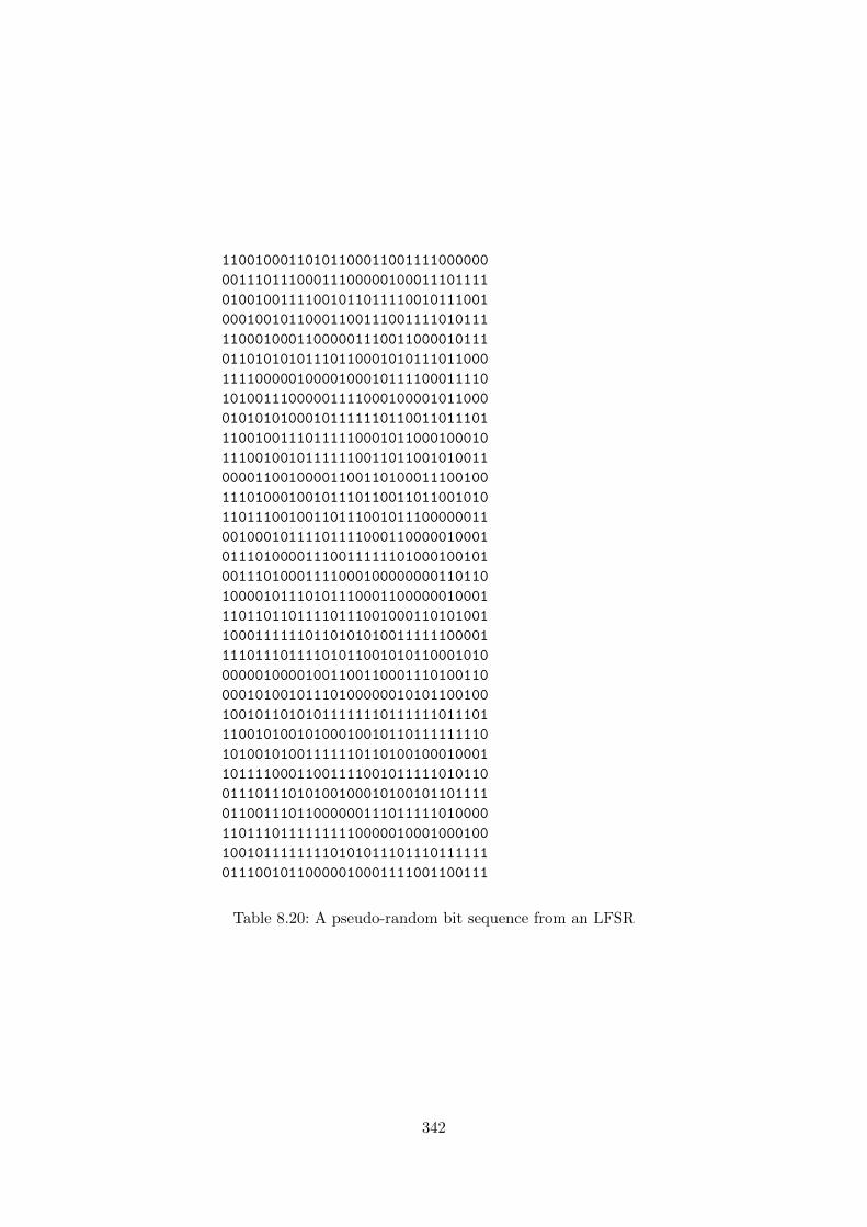
11001000110101100011001111000000
00111011100011100000100011101111
01001001111001011011110010111001
00010010110001100111001111010111
11000100011000001110011000010111
01101010101110110001010111011000
11110000010000100010111100011110
10100111000001111000100001011000
01010101000101111110110011011101
11001001110111110001011000100010
11100100101111110011011001010011
00001100100001100110100011100100
11101000100101110110011011001010
11011100100110111001011100000011
00100010111101111000110000010001
01110100001110011111101000100101
00111010001111000100000000110110
10000101110101110001100000010001
11011011011110111001000110101001
10001111110110101010011111100001
11101110111101011001010110001010
00000100001001100110001110100110
00010100101110100000010101100100
10010110101011111110111111011101
11001010010100010010110111111110
10100101001111110110100100010001
10111100011001111001011111010110
01110111010100100010100101101111
01100111011000000111011111010000
11011101111111110000010001000100
10010111111110101011101110111111
01110010110000010001111001100111
Table 8.20: A pseudo-random bit sequence from an LFSR
342
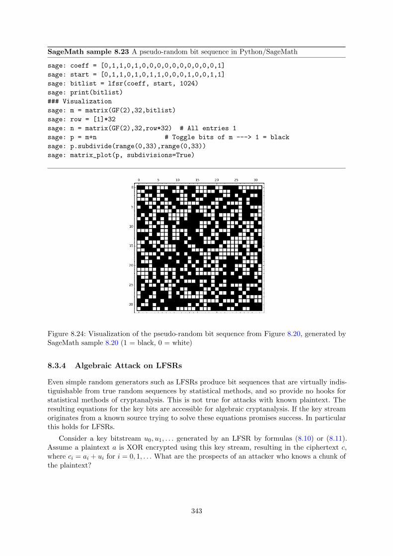
SageMath sample 8.23 A pseudo-random bit sequence in Python/SageMath
sage: coeff = [0,1,1,0,1,0,0,0,0,0,0,0,0,0,0,1]
sage: start = [0,1,1,0,1,0,1,1,0,0,0,1,0,0,1,1]
sage: bitlist = lfsr(coeff, start, 1024)
sage: print(bitlist)
### Visualization
sage: m = matrix(GF(2),32,bitlist)
sage: row = [1]*32
sage: n = matrix(GF(2),32,row*32) # All entries 1
sage: p = m+n # Toggle bits of m ---> 1 = black
sage: p.subdivide(range(0,33),range(0,33))
sage: matrix_plot(p, subdivisions=True)
Figure 8.24: Visualization of the pseudo-random bit sequence from Figure 8.20, generated bySageMath sample 8.20 (1 = black, 0 = white)
8.3.4 Algebraic Attack on LFSRs
Even simple random generators such as LFSRs produce bit sequences that are virtually indis-tiguishable from true random sequences by statistical methods, and so provide no hooks forstatistical methods of cryptanalysis. This is not true for attacks with known plaintext. Theresulting equations for the key bits are accessible for algebraic cryptanalysis. If the key streamoriginates from a known source trying to solve these equations promises success. In particularthis holds for LFSRs.
Consider a key bitstream u0, u1, . . . generated by an LFSR by formulas (8.10) or (8.11).Assume a plaintext a is XOR encrypted using this key stream, resulting in the ciphertext c,where ci = ai + ui for i = 0, 1, . . . What are the prospects of an attacker who knows a chunk ofthe plaintext?
343

Well, assume she knows the first l + 1 bits110 of the plaintext. She immediately derives thecorresponding bits u0, . . . , ul of the key stream, in particular the initial state of the LFSR. Forthe yet unknown coefficients si she knows a linear relation:
s1ul−1 + · · ·+ slu0 = ul.
Each additional known plaintext bit yields one more relation, and having l relations, from 2l bitsof known plaintext, the easy linear algebra over the field F2 (in non-degenerate cases) finds aunique solution. In the next subsections we’ll prove, using some deeper mathematical methods:
Theorem 8.3.1. An LFSR of length l is completely predictable from the first 2l bits for the costof about 1
3 · l3 bit operations.
Prediction of LFSRs
Assume we know the first 2l bits u0, . . . , u2l−1 from an LFSR of length l. For an elegantformulation of the linear algebra methods we introduce the state vectors
u(i) = (ui, . . . , ui+l−1) for i = 0, 1, . . .
The vector u(i) is the register content for step i (in reversed order compared with Figure 8.21).Thus the analysis focusses on the states, not directly on the output. The recursion (8.10) inmatrix form (for n ≥ l) is
un−l+1...
un−1un
=
0 1 . . . 0...
.... . .
...0 0 . . . 1sl sl−1 . . . s1
un−l
...un−2un−1
or more parsimoniously (the indices being substituted by m = n− l + 1)
u(m) = S · u(m−1) for m ≥ 1
where S is the coefficient matrix. As a further step we collect l consecutive state vectorsu(i), . . . , u(i+l−1) in a state matrix
U(i) =
ui ui+1 . . . ui+l−1ui+1 ui+2 . . . ui+l
......
. . ....
ui+l−1 ui+l . . . u2l−2
and set U = U(0), V = U(1). This gives the formula
V = S · U
that expresses the unknown coefficients s1, . . . , sl by the known plaintext bits u0, . . . , u2l−1. Mostnotably it allows us to write down the solution immediately—provided that the matrix U isinvertible:
S = V · U−1.The matrix S explicitly displays the coefficients s1, . . . , sl. We’ll discuss the invertibility later on.
110If she knows any l + 1 bits, even non-contiguous, the idea of attack is the same, only the formalism is slightlymore involved.
344

Example
Assume we are given a ciphertext:
10011100 10100100 01010110 10100110 01011101 10101110
01100101 10000000 00111011 10000010 11011001 11010111
00110010 11111110 01010011 10000010 10101100 00010010
11000110 01010101 00001011 11010011 01111011 10110000
10011111 00100100 00001111 01010011 11111101
We suspect that the cipher is XOR with a key stream from an LFSR of length l = 16. Thecontext suggest that the text is in German and begins with the word “Treffpunkt” (meetingpoint). To solve the cryptogram we need 32 bits of plaintext, that is the first four letters only,presupposed that the theory applies. This gives 32 bits of the key stream:
01010100 01110010 01100101 01100110 = T r e f
10011100 10100100 01010110 10100110 cipher bits
-------- -------- -------- --------
11001000 11010110 00110011 11000000 key bits
SageMath sample 8.24 determines the coefficient matrix. Its last row tells us that all si = 0except s16 = s5 = s3 = s2 = 1.
Now we know the LFSR and the initial state, and can reconstruct the complete key stream—yes, it is the same as in Figure 8.20—and write down the plaintext (that by the way begins a bitdifferently from our guess).
Proof of the Theorem
We have shown that the cofficients are uniquely determined assuming the state matrix U = U(0)
is invertible. As a consequence in this case the LFSR is completely known, and all output bitsare predictable. We have yet to discuss the case where the matrix U is singular.
If one of the first l state vectors (= rows of the matrix U) is zero, then all following statevectors are zero too, and prediction is trivial.
Thus we may assume that none of these vectors are zero, but that they are linearly dependent.Then there is a smallest index k ≥ 1 such that u(k) is contained in the subspace spanned byu(0), . . . , u(k−1), and we find coefficients t1, . . . , tk ∈ F2 such that
u(k) = t1u(k−1) + · · ·+ tku(0).
Then also u(k+1) = S ·u(k) = t1S ·u(k−1) + · · ·+ tkS ·u(0) = t1u(k) + · · ·+ tku(1), and by inductionwe get
u(n) = t1u(n−1) + · · ·+ tku(n−k) for all n ≥ k.This formula predicts all the following bits.
The statement on the cost follows from Theorem 8.1.10.
Discussion
• For a singular state matrix this consideration yields a shorter LFSR (of length k < l) thatgenerates exactly the same sequence. Then our method doesn’t determine the coefficientsof the original register but nevertheless correctly predicts the sequence.
345

SageMath sample 8.24 Determining a coefficient matrix
sage: l = 16
sage: kbits =
[1,1,0,0,1,0,0,0,1,1,0,1,0,1,1,0,0,0,1,1,0,0,1,1,1,1,0,0,0,0,0,0]
sage: ulist = []
sage: for i in range(0,l):
state = kbits[i:(l+i)]
ulist.append(state)
sage: U = matrix(GF(2),ulist)
sage: det(U)
1
sage: W = U.inverse()
sage: vlist = []
sage: for i in range(1,l+1):
state = kbits[i:(l+i)]
vlist.append(state)
sage: V = matrix(GF(2),vlist)
sage: S = V*W
sage: S
[0 1 0 0 0 0 0 0 0 0 0 0 0 0 0 0]
[0 0 1 0 0 0 0 0 0 0 0 0 0 0 0 0]
[0 0 0 1 0 0 0 0 0 0 0 0 0 0 0 0]
[0 0 0 0 1 0 0 0 0 0 0 0 0 0 0 0]
[0 0 0 0 0 1 0 0 0 0 0 0 0 0 0 0]
[0 0 0 0 0 0 1 0 0 0 0 0 0 0 0 0]
[0 0 0 0 0 0 0 1 0 0 0 0 0 0 0 0]
[0 0 0 0 0 0 0 0 1 0 0 0 0 0 0 0]
[0 0 0 0 0 0 0 0 0 1 0 0 0 0 0 0]
[0 0 0 0 0 0 0 0 0 0 1 0 0 0 0 0]
[0 0 0 0 0 0 0 0 0 0 0 1 0 0 0 0]
[0 0 0 0 0 0 0 0 0 0 0 0 1 0 0 0]
[0 0 0 0 0 0 0 0 0 0 0 0 0 1 0 0]
[0 0 0 0 0 0 0 0 0 0 0 0 0 0 1 0]
[0 0 0 0 0 0 0 0 0 0 0 0 0 0 0 1]
[1 0 0 0 0 0 0 0 0 0 0 1 0 1 1 0]
• If the bits the attacker knows aren’t just the first ones but 2l contiguous ones at a laterposition, then the theorem yields only the prediction of the following bits. In the main caseof an invertible state matrix U the LFSR is completely known and may be run backwardsto get the previous bits. For a singular state matrix we achieve the same effect using theshorter LFSR constructed above.
• The situation where 2l bits of the key stream are known but at non-contiguous positionsis slightly more involved. We get linear relations that contain additional (unknown)intermediate bits. If m is the number of these then we get l +m linear equations for l +munknown bits.
• What if the length l of the LFSR is unknown? Exhaustively trying all values l = 1, 2, 3, . . .
346

is nasty but feasible. A better approach is provided by the Berlekamp-Massey111 algorithmthat is efficient also without knowledge of l. We won’t treat it in this chapter.
Summary
Given a random generator as in Figure 8.20 cryptanalytic targets are:
• the secret parameters,
• the initial state,
• additional parts of the output (“prediction problem”),
given some parts of the output. As we saw for LFSRs the prediction problem has a solution evenwhen the internal parameters remain unknown. Thus:
Cryptanalysis of a random generator first of all means solving the prediction problem.A random generator is cryptographically secure if its prediction problem admits noefficient solution.
Linear feedback shift registers are not cryptographically secure.
8.3.5 Approaches to Nonlinearity for Feedback Shift Registers
LFSRs are popular—in particular among electrical engineers and military—for several reasons:
• very easy implementation,
• extreme efficiency in hardware,
• good qualification as random generators for statistical applications and simulations,
• unproblematic operation in parallel even in large quantities.
But unfortunately from a cryptological view they are completely insecure if used naively. Tocapitalize their positive properties while escaping their cryptological weakness there are severalapproaches.
Approach 1, Nonlinear Feedback
Nonlinear feedback follows the scheme from Figure 8.21 with a nonlinear Boolean function f . Wewon’t pursue this approach here. We saw a very simple toy example in SageMath sample 8.21.There is a general proof that in realistic use cases NLFSRs112 are cryptographically useless ifused in the direct naive way [Pom16].
Approach 2, Nonlinear Output Filter
The nonlinear ouput filter (nonlinear feedforward) realizes the scheme from Figure 8.25. Theshift register itself is linear, the Boolean function f , nonlinear.
The nonlinear ouput filter is a special case of a nonlinear combiner.
111in SageMath contained as sage.crypto.lfsr.berlekamp_massey, in CrypTool 2 under“cryptanalysis”/“generic”/“Berlekamp-Massey algorithm”
112for Non Linear Feedback Shift Register
347

����f
. . . . . .-
6
�������
������
������
�����:- -
Figure 8.25: Nonlinear ouput filter for an LFSR
. . . . . .-
. . . . . .-
......
......
-
-
�
�
�
�
-f
Figure 8.26: Nonlinear combiner
Approach 3, Nonlinear Combiner
The nonlinear combiner uses a “battery” of n LFSRs—preferably of different lengths—operated inparallel. The output sequences of the LFSRs serve as input113 of a Boolean function f: Fn2 −→ F2,see Figure 8.26. We’ll see in Section 8.3.7 how to cryptanalyze this random generator.
Approach 4, Output Selection/Decimation/Clocking
There are different ways of controlling a battery of n parallel LFSRs by another LFSR:
• Output selection takes the current output bit of exactly one of the LFSRs from the“battery”, depending on the state of the auxiliary register, and outputs it as the nextpseudo-random bit. More generally we could choose “r from n”.
• For decimation one usually takes n = 1, and outputs the current bit of the one battery
113hence the occasional denotation “nonlinear feedforward”
348
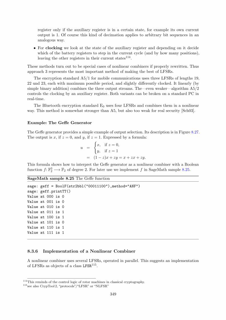
register only if the auxiliary register is in a certain state, for example its own currentoutput is 1. Of course this kind of decimation applies to arbitrary bit sequences in ananalogous way.
• For clocking we look at the state of the auxiliary register and depending on it decidewhich of the battery registers to step in the current cycle (and by how many positions),leaving the other registers in their current states114.
These methods turn out to be special cases of nonlinear combiners if properly rewritten. Thusapproach 3 represents the most important method of making the best of LFSRs.
The encryption standard A5/1 for mobile communications uses three LFSRs of lengths 19,22 und 23, each with maximum possible period, and slightly differently clocked. It linearly (bysimple binary addition) combines the three output streams. The—even weaker—algorithm A5/2controls the clocking by an auxiliary register. Both variants can be broken on a standard PC inreal-time.
The Bluetooth encryption standard E0 uses four LFSRs and combines them in a nonlinearway. This method is somewhat stronger than A5, but also too weak for real security [Sch03].
Example: The Geffe Generator
The Geffe generator provides a simple example of output selection. Its description is in Figure 8.27.The output is x, if z = 0, and y, if z = 1. Expressed by a formula:
u =
{x, if z = 0,
y, if z = 1
= (1− z)x+ zy = x+ zx+ zy.
This formula shows how to interpret the Geffe generator as a nonlinear combiner with a Booleanfunction f: F3
2 −→ F2 of degree 2. For later use we implement f in SageMath sample 8.25.
SageMath sample 8.25 The Geffe function
sage: geff = BoolF(str2bbl("00011100"),method="ANF")
sage: geff.printTT()
Value at 000 is 0
Value at 001 is 0
Value at 010 is 0
Value at 011 is 1
Value at 100 is 1
Value at 101 is 0
Value at 110 is 1
Value at 111 is 1
8.3.6 Implementation of a Nonlinear Combiner
A nonlinear combiner uses several LFSRs, operated in parallel. This suggests an implementationof LFSRs as objects of a class LFSR115.
114This reminds of the control logic of rotor machines in classical cryptography.115see also CrypTool 2, “protocols”/“LFSR” or “NLFSR”
349
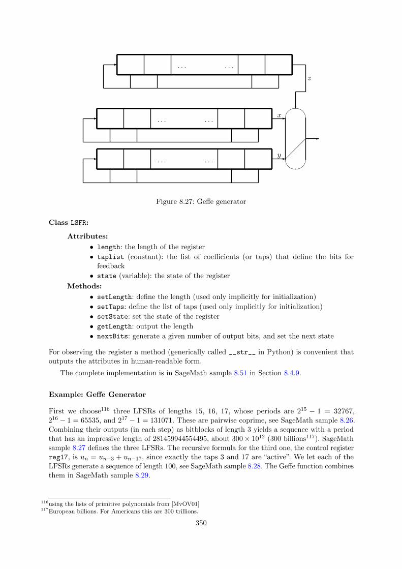
. . . . . .-
. . . . . .-
. . . . . .-
z
?
-x
-y
�
�
�
��
��
-
Figure 8.27: Geffe generator
Class LSFR:
Attributes:
• length: the length of the register
• taplist (constant): the list of coefficients (or taps) that define the bits forfeedback
• state (variable): the state of the register
Methods:
• setLength: define the length (used only implicitly for initialization)
• setTaps: define the list of taps (used only implicitly for initialization)
• setState: set the state of the register
• getLength: output the length
• nextBits: generate a given number of output bits, and set the next state
For observing the register a method (generically called __str__ in Python) is convenient thatoutputs the attributes in human-readable form.
The complete implementation is in SageMath sample 8.51 in Section 8.4.9.
Example: Geffe Generator
First we choose116 three LFSRs of lengths 15, 16, 17, whose periods are 215 − 1 = 32767,216 − 1 = 65535, and 217 − 1 = 131071. These are pairwise coprime, see SageMath sample 8.26.Combining their outputs (in each step) as bitblocks of length 3 yields a sequence with a periodthat has an impressive length of 281459944554495, about 300× 1012 (300 billions117). SageMathsample 8.27 defines the three LFSRs. The recursive formula for the third one, the control registerreg17, is un = un−3 + un−17, since exactly the taps 3 and 17 are “active”. We let each of theLFSRs generate a sequence of length 100, see SageMath sample 8.28. The Geffe function combinesthem in SageMath sample 8.29.
116using the lists of primitive polynomials from [MvOV01]117European billions. For Americans this are 300 trillions.
350

SageMath sample 8.26 Calculating a period
sage: n15 = 2**15 - 1; n15
32767
sage: n15.factor()
7 * 31 * 151
sage: n16 = 2**16 - 1; n16
65535
sage: n16.factor()
3 * 5 * 17 * 257
sage: n17 = 2**17 - 1; n17
131071
sage: n17.factor()
131071
sage: period = n15 * n16 * n17; period
281459944554495
SageMath sample 8.27 Three LFSRs
sage: reg15 = LFSR([1,0,0,0,0,0,0,0,0,0,0,0,0,0,1])
sage: reg15.setState([0,1,1,0,1,0,1,1,0,0,0,1,0,0,1])
sage: print(reg15)
Length: 15 | Taps: 100000000000001 | State: 011010110001001
sage: reg16 = LFSR([0,1,1,0,1,0,0,0,0,0,0,0,0,0,0,1])
sage: reg16.setState([0,1,1,0,1,0,1,1,0,0,0,1,0,0,1,1])
sage: print(reg16)
Length: 16 | Taps: 0110100000000001 | State: 0110101100010011
sage: reg17 = LFSR([0,0,1,0,0,0,0,0,0,0,0,0,0,0,0,0,1])
sage: reg17.setState([0,1,1,0,1,0,1,1,0,0,0,1,0,0,1,1,1])
sage: print(reg17)
Length: 17 | Taps: 00100000000000001 | State: 01101011000100111
351

SageMath sample 8.28 Three LFSR sequences
sage: nofBits = 100
sage: outlist15 = reg15.nextBits(nofBits)
sage: print(outlist15)
[1, 0, 0, 1, 0, 0, 0, 1, 1, 0, 1, 0, 1, 1, 0, 1, 1, 1, 0, 0,
0, 0, 1, 0, 0, 1, 1, 0, 1, 1, 0, 1, 0, 0, 0, 0, 0, 1, 1, 1,
0, 1, 1, 0, 1, 1, 0, 0, 0, 0, 0, 0, 1, 0, 1, 1, 0, 1, 1, 0,
1, 1, 1, 1, 1, 1, 1, 0, 0, 1, 0, 0, 1, 0, 0, 1, 0, 1, 0, 1,
0, 1, 1, 1, 0, 0, 0, 1, 1, 1, 0, 0, 1, 1, 0, 0, 1, 0, 1, 1]
sage: outlist16 = reg16.nextBits(nofBits)
sage: print(outlist16)
[1, 1, 0, 0, 1, 0, 0, 0, 1, 1, 0, 1, 0, 1, 1, 0, 0, 0, 1, 1,
0, 0, 1, 1, 1, 1, 0, 0, 0, 0, 0, 0, 0, 0, 1, 1, 1, 0, 1, 1,
1, 0, 0, 0, 1, 1, 1, 0, 0, 0, 0, 0, 1, 0, 0, 0, 1, 1, 1, 0,
1, 1, 1, 1, 0, 1, 0, 0, 1, 0, 0, 1, 1, 1, 1, 0, 0, 1, 0, 1,
1, 0, 1, 1, 1, 1, 0, 0, 1, 0, 1, 1, 1, 0, 0, 1, 0, 0, 0, 1]
sage: outlist17 = reg17.nextBits(nofBits)
sage: print(outlist17)
[1, 1, 1, 0, 0, 1, 0, 0, 0, 1, 1, 0, 1, 0, 1, 1, 0, 0, 0, 1,
0, 0, 0, 0, 0, 0, 1, 1, 0, 0, 1, 1, 1, 1, 1, 1, 0, 1, 1, 0,
1, 1, 0, 0, 0, 0, 0, 1, 1, 1, 0, 0, 0, 0, 1, 1, 0, 0, 0, 0,
0, 0, 0, 0, 1, 1, 1, 1, 1, 1, 1, 0, 0, 1, 0, 0, 1, 0, 0, 1,
0, 1, 0, 1, 0, 1, 0, 1, 1, 0, 0, 1, 0, 1, 1, 0, 0, 1, 1, 0]
352

SageMath sample 8.29 The combined sequence
sage: outlist = []
sage: for i in range(0,nofBits):
....: x = [outlist15[i],outlist16[i],outlist17[i]]
....: outlist.append(geff.valueAt(x))
....:
sage: print(outlist)
[1, 1, 0, 1, 0, 0, 0, 1, 1, 1, 0, 0, 0, 1, 1, 0, 1, 1, 0, 1,
0, 0, 1, 0, 0, 1, 0, 0, 1, 1, 0, 0, 0, 0, 1, 1, 0, 0, 1, 1,
1, 0, 1, 0, 1, 1, 0, 0, 0, 0, 0, 0, 1, 0, 0, 0, 0, 1, 1, 0,
1, 1, 1, 1, 0, 1, 0, 0, 1, 0, 0, 0, 1, 1, 0, 1, 0, 1, 0, 1,
0, 0, 1, 1, 0, 1, 0, 0, 1, 1, 0, 1, 1, 0, 0, 0, 1, 0, 0, 1]
8.3.7 Correlation Attacks—the Achilles Heels of Combiners
Let f: Fn2 −→ F2 be the combining function of a nonlinear combiner. The number
Kf := #{x = (x1, . . . , xn) ∈ Fn2 | f(x) = x1}
counts the coincidences of the value of the function with its first argument. If it is > 2n−1, thenthe probability of a coincidence,
p =1
2n·Kf >
1
2,
is above average, and the combined output sequence “correlates” with the output of the firstLFSR more then expected by random. If p < 1
2 , then the correlation deviates from the expectedvalue in the other direction.
The cryptanalyst can exploit this effect in an attack with known plaintext. We suppose thatshe knows the “hardware”, that is the taps of the registers, and also the combining function f .She seeks the initial states of all the LFSRs. We assume she knows the bits k0, . . . , kr−1 of thekey stream118. For each of the 2l1 initial states of the first LFSR she generates the sequenceu0, . . . , ur−1, and counts the coincidences. The expected values are
1
r·#{i | ui = ki} ≈
{p for the correct initial state of LFSR 1,12 otherwise.
If r is large enough, she can determine the true initial state of LFSR 1 (with high probability)for a cost of ∼ 2l1 . She continues with the other registers, and finally identifies the complete keywith a cost of ∼ 2l1 + · · ·+ 2ln . Note that the cost is exponential, but significantly lower thanthe cost ∼ 2l1 · · · 2ln of the naive exhaustion of the key space.
In the language of linear cryptanalysis from 8.2.6 she made use of the linear relation
f(x1, . . . , xn)p≈ x1
for f . Clearly she could use any linear relation as well to reduce the complexity of key search119.
118for simplicity of exposition the first ones. The argument works in the same way for any r known key bits.119A more in-depth analysis of the situation leads to the notion of correlation immunity that is related with the
linear potential.
353

Correlations from the Geffe Generator
From the truth table 8.21 we get the correlations produced by the Geffe generator. Thus theprobabilities of coincidences are
p =
34 for register 1 (x),34 for register 2 (y),12 for register 3 (z = control bit).
A correlation attack easily detects the initial states of registers 1 and 2—the battery registers—given only a short piece of an output sequence. Afterwards exhaustion finds the initial state ofregister 3, the control register.
x 0 0 0 0 1 1 1 1y 0 0 1 1 0 0 1 1z 0 1 0 1 0 1 0 1
f(x, y, z) 0 0 0 1 1 1 0 1
Table 8.21: Truth table of the Geffe function (in horizontal order)
We exploit this weakness of the Geffe generator in SageMath sample 8.30 that continuesSageMath sample 8.25. Since we defined the linear profile for objects of the class BoolMap only,we first of all have to interpret the function geff as a Boolean map, that is a one-element listof Boolean functions. Then the linear profile is represented by a matrix of 2 columns and 8rows. The first column [64, 0, 0, 0, 0, 0, 0, 0] shows the coincidences with the linearform 0 in the range. So it contains no useful information, except the denominator 64 that appliesto all entries. The second row [0, 0, 16, 16, 16, 16, 0, 0] yields the list of coincidenceprobabilities p (after dividing it by 64) in Table 8.22, using the formula
p =1
2· (±√λ+ 1).
If λ = 0, then p = 1/2. If λ = 1/4, then p = 1/4 or 3/4. For deciding between these twovalues for p we use Table 8.21.
linear form 0 z y y + z x x+ z x+ y x+ y + zrepresentation 000 001 010 011 100 101 110 111
potential 0 0 1/4 1/4 1/4 1/4 0 0probability p 1/2 1/2 3/4 1/4 3/4 3/4 1/2 1/2
Table 8.22: Coincidence probabilities of the Geffe function
SageMath sample 8.30 Linear profile of the Geffe function
sage: g = BoolMap([geff])
sage: linProf = g.linProf(); linProf
[[64,0], [0,0], [0,16], [0,16], [0,16], [0,16], [0,0], [0,0]]
In SageMath sample 8.31 we apply this finding to the 100 element sequence from SageMathsample 8.29. The function coinc from SageMath sample 8.39 (in the appendix) counts the
354

coincidences. For the first register we find 73 coincidences, for the second one 76, for the thirdone only 41. This confirms the values 75, 75, 50 predicted by our theory (taking into accountstatistical variability).
SageMath sample 8.31 Coincidences for the Geffe generator
sage: coinc(outlist15,outlist)
73
sage: coinc(outlist16,outlist)
76
sage: coinc(outlist17,outlist)
41
Cryptanalysis of the Geffe Generator
These results promise an effortless analysis of our sample sequence. For an assessment of thesuccess probability we consider a bitblock b ∈ Fr2 and first ask how large is the probability that arandom bitblock u ∈ Fr2 coincides with b at exactly t positions. For an answer we have to look atthe symmetric binomial distribution (where p = 1
2 is the probability of coincidence at a singleposition): The probability of exactly t coincidences is
Br, 12(t) =
(rt
)2r.
Hence the cumulated probability of up to T coincidences is
T∑t=0
Br, 12(t) =
1
2r·T∑t=0
(r
t
).
If r is not too large, then we may explicitly calculate this value for a given bound T . If on theother hand r is not too small, then we approximate the value using the normal distribution. Themean value of the number of coincidences is r/2, the variance, r/4, and the standard deviation,√r/2.
In any case for r = 100 the probability of finding at most (say) 65 coincidences is 0.999, theprobability of surpassing this number is 1 h. For the initial state of register 1 we have to try215 = 32786 possibilities (generously including the zero state 0 ∈ F15
2 into the count). So weexpect about 33 oversteppings with at least 66 coincidences. One of these should occur for thetrue initial state of register 1 that we expect to produce about 75 coincidences. Maybe it evenproduces the maximum number of coincidences.
SageMath sample 8.32 shows that this really happens. However the maximum number ofcoincidences, 73, occurs twice in the histogram. The first occurrence happens at index 13705,corresponding to the initial state 011010110001001, the correct solution. The second occurrence,at index 31115, see SageMath sample 8.33, yields the false solution 111100110001011 thateventually leads to a contradiction.
SageMath sample 8.34 shows the analogous analysis of register 2. Here the maximum of coin-cidences, 76, is unique, occurs at index 27411 corresponding to the initial state 0110101100010011,and provides the correct solution.
To complete the analysis we must yet determine the initial state of register 3, the controlregister. The obvious idea is to exhaust the 217 different possibilities. There is a shortcut since
355

SageMath sample 8.32 Analysis of the Geffe generator—register 1
sage: clist = []
sage: histogr = [0] * (nofBits + 1)
sage: for i in range(0,2**15):
....: start = int2bbl(i,15)
....: reg15.setState(start)
....: testlist = reg15.nextBits(nofBits)
....: c = coinc(outlist,testlist)
....: histogr[c] += 1
....: clist.append(c)
....:
sage: print(histogr)
[0, 0, 0, 0, 0, 0, 0, 0, 0, 0, 0, 0, 0, 0, 0, 0, 0, 0, 0, 0, 0,
0, 0, 0, 0, 0, 0, 0, 0, 0, 0, 0, 0, 4, 12, 12, 37, 78, 116, 216,
329, 472, 722, 1003, 1369, 1746, 1976, 2266, 2472, 2531, 2600,
2483, 2355, 2149, 1836, 1574, 1218, 928, 726, 521, 343, 228, 164,
102, 60, 47, 36, 13, 8, 7, 4, 2, 1, 2, 0, 0, 0, 0, 0, 0, 0, 0, 0,
0, 0, 0, 0, 0, 0, 0, 0, 0, 0, 0, 0, 0, 0, 0, 0, 0, 0]
sage: mm = max(clist)
sage: ix = clist.index(mm)
sage: block = int2bbl(ix,15)
sage: print "Maximum =", mm, "at index", ix, ", start value", block
Maximum = 73 at index 13705 , start value\
[0, 1, 1, 0, 1, 0, 1, 1, 0, 0, 0, 1, 0, 0, 1]
SageMath sample 8.33 Analysis of the Geffe generator—continued
sage: ix = clist.index(mm,13706); ix
31115
sage: print int2bbl(ix,15)
[1, 1, 1, 1, 0, 0, 1, 1, 0, 0, 0, 1, 0, 1, 1]
we already know 51 of the first 100 bits of the control register: At a position where the values ofregisters 1 and 2 differ, the control bit is necessarily 0 if the final output coincides with register1, and 1 otherwise. Only at positions where registers 1 and 2 coincide the corresponding bit ofregister 3 is undetermined.
register 1: 10010001101011011100001001101101000001110110110000
register 2: 11001000110101100011001111000000001110111000111000
register 3: -1-00--0-1101-110001---00-1-00-1--1101--110---0---
bitsequence: 11010001110001101101001001001100001100111010110000
... 00101101101111111001001001010101110001110011001011
... 00100011101111010010011110010110111100101110010001
... ----110-------1-1-11-0-100----01--01-1-001-1-00-1-
... 00100001101111010010001101010100110100110110001001
In particular we already know 11 of the 17 initial bits, and are left with only 26 = 64 possibilities
356

SageMath sample 8.34 Analysis of the Geffe generator—register 2
sage: clist = []
sage: histogr = [0] * (nofBits + 1)
sage: for i in range(0,2**16):
....: start = int2bbl(i,16)
....: reg16.setState(start)
....: testlist = reg16.nextBits(nofBits)
....: c = coinc(outlist,testlist)
....: histogr[c] += 1
....: clist.append(c)
....:
sage: print(histogr)
[0, 0, 0, 0, 0, 0, 0, 0, 0, 0, 0, 0, 0, 0, 0, 0, 0, 0, 0, 0,
0, 0, 0, 0, 0, 0, 0, 1, 0, 2, 3, 4, 8, 17, 25, 51, 92, 171,
309, 477, 750, 1014, 1423, 1977, 2578, 3174, 3721, 4452, 4821,
5061, 5215, 5074, 4882, 4344, 3797, 3228, 2602, 1974, 1419,
1054, 669, 434, 306, 174, 99, 62, 38, 19, 10, 3, 0, 1, 0, 0,
0, 0, 1, 0, 0, 0, 0, 0, 0, 0, 0, 0, 0, 0, 0, 0, 0, 0, 0, 0,
0, 0, 0, 0, 0, 0, 0]
sage: mm = max(clist)
sage: ix = clist.index(mm)
sage: block = int2bbl(ix,16)
sage: print "Maximum =", mm, "at index", ix, ", start value", block
Maximum = 76 at index 27411 , start value\
[0, 1, 1, 0, 1, 0, 1, 1, 0, 0, 0, 1, 0, 0, 1, 1]
to try.
But even this may be further simplified, since the known and the unknown bits obey linearrelations of the type un = un−3 + un−17. The unknown bits of the initial state are u0, u2, u5, u6,u8, u13. The solution follows the columns of Table 8.23, that immediately give
u0 = 1, u2 = 1, u6 = 0.
The remaining solutions are
u8 = u22 = u39 = 0, u5 = u22 + 1 = u8 + 1 = 1, u13 = u30 + 1 = 0.
Hence the initial state of the control register is 01101011000100111, and we know this is thecorrect solution. We don’t need to bother with the second possible solution for register 1 sincewe already found a constellation that correctly reproduces the sequence.
8.3.8 Design Criteria for Nonlinear Combiners
From the forgoing discussion we derive design criteria for nonlinear combiners:
• The battery registers should be as long as possible.
• The combining function f should have a low linear potential.
357

u17 = u14 + u0 0 = 1 + u0 u0 = 1u19 = u16 + u2 1 = 0 + u2 u2 = 1u20 = u17 + u3 u20 = 0 + 0 u20 = 0u22 = u19 + u5 u22 = u5 + 1 u5 = u22 + 1u23 = u20 + u6 0 = u20 + u6 u6 = u20 u6 = 0u25 = u22 + u8 u25 = u22 + u8 u8 = u22 + u25 u8 = u22u27 = u24 + u10 u27 = 0 + 1 u27 = 1u28 = u25 + u11 0 = u25 + 0 u25 = 0u30 = u27 + u13 u30 = u27 + u13 u13 = u27 + u30 u13 = u30 + 1u33 = u30 + u16 u33 = u30 + 0 u30 = u33 u30 = 1u36 = u33 + u19 0 = u33 + 1 u33 = 1u39 = u36 + u22 u39 = 0 + u22 u22 = u39u42 = u39 + u25 0 = u39 + u25 u39 = u25 u39 = 0
Table 8.23: Determination of the control register’s initial state
How long should the battery registers be? There are some algorithms for “fast” correlationattacks using the Walsh transformation, in particular against sparse linear feedback functions(that use only a small number of taps) [MS89]. These don’t reduce the complexity class of theattack (“exponential in the length of the shortest register”) but reduce the cost by a significantfactor. So they are able to attack registers whose feedback functions have up to 100 monomialswith coefficients in their ANF. As a consequence
• The single LFSRs should have a length of at least 200 bits, and use about 100 taps each.
To assess the number n of LFSRs we bear in mind that the combining function should be“correlation immune”, in particular have a low linear potential. A well-chosen Boolean functionof 16 variables should suffice120.
Rueppel121 found an elegant way out to make the correlation attack break down: Use a“time-dependent” combining function, that is a family (ft)t∈N. The bit ut of the key stream iscalculated by the function ft. We won’t analyze this approach here.
Observing that the correlation attack needs knowledge of the taps, the security could besomewhat better if the taps are secret. Then the attacker has to perform additional exhaustionsthat multiply the complexity by factors such as 2l1 for the first LFSR alone. This scenarioallows choosing LFSRs of somewhat smaller lengths. But bear in mind that for a hardwareimplementation the taps are parts of the algorithm, not of the key, that is they are publicparameters in the sense of Figure 8.20.
Efficiency
LFSRs and nonlinear combiners allow efficient realizations by special hardware that producesone bit per clock cycle. This rate can be enlarged by parallelization. From this point of viewestimating the cost of execution on a usual PC processor is somewhat inadequate. Splitting eachof the ≥ 200 bit registers into 4 parts of about 64 bits shifting a single register requires at least4 clock cycles, summing up to 64 clock cycles for 16 registers. Add some clock cycles for the
120There are no known recommendations in the literature.121Rainer A. Rueppel, Swiss cryptographer
358

combining function. Thus one single bit would take about 100 clock cycles. A 2-GHz processor,even with optimized implementation, would produce at most 2 · 109/100 = 20 million bits persecond.
As a summary we note:
Using LFSRs and nonlinear combining functions we can build useful and fast randomgenerators, especially in hardware.
Unfortunately there is no satisfying theory for the cryptologic security of this type of randomgenerators, even less a mathematical proof. Security is assessed by plausible criteria that—as forbitblock ciphers—are related to the nonlinearity of Boolean functions.
8.3.9 Perfect (Pseudo-)Random Generators
As we saw the essential cryptologic criterion for random generators is unpredictability. In the1980s cryptographers, guided by an analogy with asymmetric cryptography, found a way ofmodelling this property in terms of complexity theory: Prediction should boil down to a known“hard” algorithmic problem such as factoring or discrete logarithm. This idea established a newquality standard for random generators, much stronger than statistical tests, but eventuallybuilding on unproven mathematical hypotheses. Thus the situation with respect to the securityof random generators is comparable to asymmetric encryption.
As an interesting twist it soon turned out that in a certain sense unpredictability is a universalproperty: For an unpredictable sequence there is no efficient algorithm at all that distinguishesit from a true random sequence, a seemingly much stronger requirement. See Theorem 8.3.2(Yao’s theorem). This universality justifies the denomination “perfect” for the correspondingrandom generators. In particular there is no efficient statistical test that is able to distinguishthe output of a perfect random generator from a true random sequence. Thus, on the theoreticalside, we have a very appropriate model for random generators that are absolutely strong from astatistical viewpoint, and invulnerable from a cryptological viewpoint. In other words:
Perfect random generators are cryptographically secure and statistically undistin-guishable from true random sources.
Presumably perfect random generators exist, but there is no complete mathematicalproof ot their existence.
The first concrete approaches to the construction of perfect random generators, the best knownbeing the BBS generator (for Blum122, Blum123, Shub124), yielded algorithms that were too slowfor most practical uses (given the then current CPUs). But modified approaches soon providedrandom generators that are passably fast und nevertheless (presumably) cryptographically secure.
8.3.10 The BBS Generator
As with the RSA cipher we consider an integer module m that is a product of two large primenumbers. For the BBS generator we choose125 Blum primes p; these are primes ≡ 3 mod 4. Aproduct of two Blum primes is called a Blum integer.
122Lenore Blum, U. S. American mathematician and computer scientist, *December 18, 1942123Manuel Blum, U. S. American mathematician and computer scientist, *April 26, 1938124Michael Shub, U. S. American mathematician, *August 17, 1943125for technical reasons not to be discussed here
359

The BBS generator works in the following way: As a first step choose two large random Blumprimes p and q, and form their product m = pq. As a second step choose a random integer seeds with 1 ≤ s ≤ m− 1, and coprime126,127 with m.
Now we proceed with generating a pseudo-random sequence: Take x0 = s2 mod m as initialstate128, and form the sequence of inner states of the random generator: xi = x2i−1 mod m fori = 1, 2, 3, . . . In each step output that last significant bit of the binary representation, that isui = xi mod 2 for i = 0, 1, 2, . . ., or in other words, the parity of xi.
Example
Of course an example with small numbers is practically irrelevant, but it illustrates the algorithm:Take p = 7, q = 11, m = 77, s = 53. Then s2 = 2809, hence x0 = 37, and u0 = 1 since x0 is odd.The naive SageMath sample 8.35 shows the beginning of the sequence of states:
i 0 1 2 3 . . .
xi 37 60 58 53 . . .ui 1 0 0 1 . . .
SageMath sample 8.35 A (much too) simple example for BBS
sage: p = 7
sage: q = 11
sage: m = p*q; m
77
sage: s = 53
sage: x0 = (s^2) % m; x0
37
sage: x1 = (x0^2) % m; x1
60
sage: x2 = (x1^2) % m; x2
58
sage: x3 = (x2^2) % m; x3
53
Treating the Blum primes p and q as secret is essential for the security of the BBS generator.They serve for forming m only, afterwards they may even be destroyed. In contrast with RSAthere is no further use for them. Likewise all the non-output bits of the inner states xi must besecret.
The standard distribution of SageMath contains the BBS generator. It consists of theprocedures:
• random_blum_prime() in the module sage.crypto.util. To generate a random Blumprime p with a given number k of bits (= digits of the binary representation) call it
126If we catch an s not coprime with m, we have factorized m by hazard. This might happen, but is extremelyunlikely, and can easily be captured at initialization time.
127If xi <√m, then x2
i mod m = x2i , the integer square, so x2
i+1 has the same parity as xi. In order to avoid aconstant segment at the beginning of the output, often the boundary area s <
√m, as well as s > m−
√m, is
excluded. However if we really choose s as a true random value, the probability for s falling into these boundaryareas is extremely low. But to be on the safe side we may require
√m ≤ s ≤ m−
√m.
128We want x0 to be a quadratic residue.
360
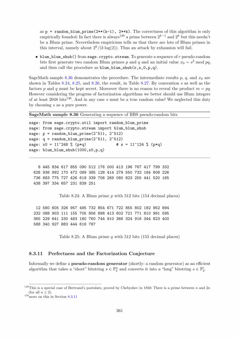
as p = random_blum_prime(2**(k-1), 2**k). The correctness of this algorithm is onlyempirically founded: In fact there is always129 a prime between 2k−1 and 2k but this needn’tbe a Blum prime. Nevertheless empiricism tells us that there are lots of Blum primes inthis interval, namely about 2k/(k log(2)). Thus an attack by exhausion will fail.
• blum_blum_shub() from sage.crypto.stream. To generate a sequence of r pseudo-randombits first generate two random Blum primes p and q and an initial value x0 = s2 mod pq,and then call the procedure as blum_blum_shub(r,x_0,p,q).
SageMath sample 8.36 demonstrates the procedure. The intermediate results p, q, and x0 areshown in Tables 8.24, 8.25, and 8.26, the result, in Table 8.27. By convention s as well as thefactors p and q must be kept secret. Moreover there is no reason to reveal the product m = pq.However considering the progress of factorization algorithms we better should use Blum integersof at least 2048 bits130. And in any case s must be a true random value! We neglected this dutyby choosing s as a pure power.
SageMath sample 8.36 Generating a sequence of BBS pseudo-random bits
sage: from sage.crypto.util import random_blum_prime
sage: from sage.crypto.stream import blum_blum_shub
sage: p = random_blum_prime(2^511, 2^512)
sage: q = random_blum_prime(2^511, 2^512)
sage: x0 = 11^248 % (p*q) # s = 11^124 % (p*q)
sage: blum_blum_shub(1000,x0,p,q)
8 445 834 617 855 090 512 176 000 413 196 767 417 799 332
626 936 992 170 472 089 385 128 414 279 550 732 184 808 226
736 683 775 727 426 619 339 706 269 080 823 255 441 520 165
438 397 334 657 231 839 251
Table 8.24: A Blum prime p with 512 bits (154 decimal places)
12 580 605 326 957 495 732 854 671 722 855 802 182 952 894
232 088 903 111 155 705 856 898 413 602 721 771 810 991 595
365 229 641 230 483 180 760 744 910 366 324 916 344 823 400
588 340 927 883 444 616 787
Table 8.25: A Blum prime q with 512 bits (155 decimal places)
8.3.11 Perfectness and the Factorization Conjecture
Informally we define a pseudo-random generator (shortly: a random generator) as an efficientalgorithm that takes a “short” bitstring s ∈ Fn2 and converts it into a “long” bitstring s ∈ Fr2.
129This is a special case of Bertrand’s postulate, proved by Chebyshev in 1850: There is a prime between n and 2n(for all n ≥ 2).
130more on this in Section 8.3.11
361

1 842 408 460 334 540 507 430 929 434 383 083 145 786 026
412 146 359 363 362 017 837 922 966 741 162 861 257 645 571
680 482 798 249 771 263 305 761 292 545 408 040 659 753 561
970 871 645 393 254 757 072 936 076 922 069 587 163 804 708
256 246 366 137 431 776 175 309 050 064 068 198 002 904 756
218 898 942 856 431 647 438 473 529 312 261 281
Table 8.26: An initial value x0
1010 0110 0011 0100 0000 0111 1111 0100 1111 0111 0010 1001
0000 0100 1111 0000 0010 1010 1011 1111 1000 0101 1110 0011
1110 1000 1001 1100 1000 1000 0110 0111 0011 0011 1010 0011
1100 1111 0011 1000 1011 0110 1011 1110 0110 1110 0111 1000
1101 0011 1101 0010 1000 1101 0000 1100 0100 1011 1110 0011
0110 0010 1011 0000 1010 1001 0110 0000 0011 1010 0011 1111
1010 0110 0101 1000 1011 0100 0100 1111 1010 1011 0001 1100
0000 0011 1101 1001 0001 0000 1111 1010 1001 0111 0111 0111
0000 1010 0101 0111 0111 0001 0110 1001 0011 1011 0000 0011
1000 0000 0111 0110 0110 1010 0110 0011 0111 1100 0010 0110
0011 1001 1010 1111 0001 0010 1111 0010 1100 1111 0110 0100
0001 1000 0101 0011 0000 0101 1111 1100 0101 0000 0100 0100
0100 0101 0010 1110 1010 1011 1011 0110 0101 1011 1111 1110
1100 1001 1011 0110 1001 0111 0111 1110 0101 0111 0011 0100
1101 1110 0011 1111 1101 0100 1111 1011 1010 0010 0111 1111
1010 1000 1100 1001 1010 1001 1010 0111 0100 0100 1010 0110
0011 0010 1110 0111 0101 0111 1101 0000 0110 0000 1110 1100
0101 1010 0111 1000 0101 1111 0010 1101 0110 0100 0010 1101
0000 1101 0111 1011 0010 1010 1000 0110 0100 0111 1100 0000
1101 0000 1011 1111 0101 1011 0011 1110 0010 1110 1101 0001
1110 1111 1000 0111 1010 0000 1100 0101 0110 0001
Table 8.27: 1000 BBS pseudo-random bits
362

The terminology of complexity theory allows us to give a mathematically exact131 definition
by considering parameter-dependent families of Boolean maps Gn : Fn2 −→ Fr(n)2 , and analyzingtheir behaviour when the parameter n grows to infinity. Such an algorithm—represented by thefamily (Gn) of Boolean maps—can be efficient only if the “expanding function” r : N −→ N growsat most polynomially with the parameter n, otherwise even writing down the output sequencein an efficient way is impossible. Then we measure the cost somehow in a meaningful way, forexample count the number of needed bit operations that likewise must be at most polynomialwith respect to the asymptotic behaviour.
On the attacker’s side we consider algorithms that predict further bits, or aim at detectingsome other weaknesses of our random generator. We analyze the costs of these algorithms alsoas functions of n. In case the cost grows faster than any polynomial, say exponentially, we ratethe attack as inefficient.
Pursuing this approach would require a lot of additional formalisms including a model ofprobabilistic algorithms that are essential tools for the cryptanalyst. This would take us tofar apart for the moment being. However we bear in mind that there is a mathematicallycorrect theory formalizing the intuitive idea of efficiency. Relying on this knowledge we don’thesitate to reasoning the naive way, and draft the following definition that in the given form ismathematically incorrect but might be made correct.
Definition 8.3.1. Consider a pseudo-random generator. A next bit predictor is an algorithmthat takes a piece u0, . . . , ur−1 from the beginning of the pseudo-random sequence and calculatesthe next bit ur, without using the internal parameters of the pseudo-random generator.
The pseudo-random generator passes the prediction test if there is no efficient next bitpredictor.
For example LFSRs don’t pass the prediction test: We constructed an efficient next bitpredictor in Theorem 8.3.1.
Definition 8.3.2. Consider a pseudo-random generator. A distinguisher is an algorithmthat decides whether a given sequence is purely random or is generated by the pseudo-randomgenerator, without using the internal parameters of the pseudo-random generator.
The pseudo-random generator is perfect if there is no efficient distinguisher for it.
In particular no efficient statistical test is able to distinguish a perfect pseudo-randomgenerator from a true random source. It is a bit of a surprise that the seemingly much weakerproperty of passing the prediction test already implies perfectness. In other words the predictiontest is “universal”:
Theorem 8.3.2. (Yao’s132 criterion) A pseudo-random generator is perfect if and only if itpasses the prediction test.
Stated without proof.
Unfortunately this approach only gives qualitative results, and so it is somewhat dissatisfying.However, as often in complexity theory, this is the best we can achieve.
The (Conjectured) Perfectness of the BBS Generator
The factorization hypothesis states that there is no efficient algorithm that decomposes largenatural numbers into their prime factors. This hypothesis is the base of the security of RSA, as
131but not completey satisfying from a practical point of view132Andrew Yao (Yao Qızhı), Chinese American computer scientist, *December 24, 1946
363

well, as stated in Theorem 8.3.3, of the perfectness of the BBS generator:
Theorem 8.3.3. (Blum/Blum/Shub/Vazirani133/Vazirani134) Assume the factorization hy-pothesis holds. Then the BBS generator is perfect.
We omit the proof (that is quite involved). Sloppily expressed the theorem says:
Whoever is able to predict a single bit of a BBS sequence given a partial sequence isalso able to factor the module.
This statement assumes that the attacker knows the module m of the BBS generator. Howeverthe module might also be secret, that is, considered as a part of the key. Assuming this thecryptographic security of BBS should even be better—but no proof of this stronger statementseems to be known, not even an informal one.
8.3.12 Examples and Practical Considerations
We saw that the BBS generator is perfect under a plausible but unproven assumption, thefactorization hypothesis. However we don’t know relevant concrete details, for example whatparameters might be inappropriate. We know that certain initial states generate output sequenceswith short periods. Some examples of this effect are known, but we are far from a completeanswer. However the security proof (depending on the factorization hypothesis) doesn’t requireadditional assumptions. Therefore we may confidently use the BBS generator with a pragmaticattitude: randomly choosing the parameters (primes and initial state) the probability of hitting“bad” values is extremely low, much lower then finding a needle in a haystack, or even in theuniverse.
Nevertheless some questions are crucial for getting good pseudo-random sequences from theBBS generator in an efficient way:
• How large should we choose the module m?
• How many bits can we use for a fixed module and initial state without compromising thesecurity?
The provable results—relative to the factorization hypothesis—are qualitative only, notquantitative. The recommendation to choose a module that escapes the known factorizationmethods also rests on heuristic considerations only, and doesn’t seem absolutely mandatory fora module that itself is kept secret. The real quality of the pseudo-random bit sequence, be it forstatistical or for cryptographic applications, can only be assessed by empirical criteria for thetime being. We are confident that the danger of generating a “bad” pseudo-random sequenceis extremely small135, in any case negligeable, for modules that escape the presently knownfactorization algorithms, say at least of a length of 2048 bits, and for a true random choice ofthe module and the initial state.
For the length of the useable output sequence we only know the qualitative criterion “atmost polynomially many” that is useless in a concrete application. But even if we only use
133Umesh Vazirani, Indian-U. S. American computer scientist134Vijay Vazirani, Indian-U. S. American computer scientist, ∗April 20, 1957135Emile Borel (Felix Edouard Justin Emile Borel, French mathematician and politician, January 7, 1871 – February
3, 1956) proposed an informal ranking of negligeability of extremely small probabilities: ≤ 10−6 from a humanview; ≤ 10−15 from a terrestrial view; ≤ 10−45 from a cosmic view. By choosing a sufficiently large module m forRSA or BBS we easily undercut Borel’s bounds by far.
364
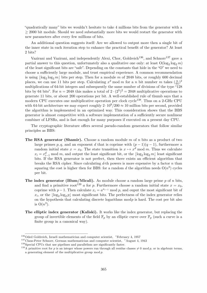
“quadratically many” bits we wouldn’t hesitate to take 4 millions bits from the generator with a≥ 2000 bit module. Should we need substantially more bits we would restart the generator withnew parameters after every few millions of bits.
An additional question suggests itself: Are we allowed to output more then a single bit ofthe inner state in each iteration step to enhance the practical benefit of the generator? At least2 bits?
Vazirani and Vazirani, and independently Alexi, Chor, Goldreich136, and Schnorr137 gave apartial answer to this question, unfortunately also a qualitative one only: at least O(log2 log2m)of the least significant bits are “safe”. Depending on the constants that hide in the “O” we need tochoose a sufficiently large module, and trust empirical experience. A common recommendationis using blog2 log2mc bits per step. Then for a module m of 2048 bits, or roughly 600 decimalplaces, we can use 11 bits per step. Calculating x2 mod m for a n bit number m takes ( n64)2
multiplications of 64-bit integers and subsequently the same number of divisions of the type “128bits by 64 bits”. For n = 2048 this makes a total of 2 · (25)2 = 2048 multiplicative operations togenerate 11 bits, or about 200 operations per bit. A well-established rule of thumb says that amodern CPU executes one multiplicative operation per clock cycle138. Thus on a 2-GHz CPUwith 64-bit architecture we may expect roughly 2 ·109/200 ≈ 10 million bits per second, providedthe algorithm is implemented in an optimized way. This consideration shows that the BBSgenerator is almost competitive with a software implementation of a sufficiently secure nonlinearcombiner of LFSRs, and is fast enough for many purposes if executed on a present day CPU.
The cryptographic literature offers several pseudo-random generators that follow similarprinciples as BBS:
The RSA generator (Shamir). Choose a random module m of n bits as a product of twolarge primes p, q, and an exponent d that is coprime with (p− 1)(q − 1), furthermore arandom initial state x = x0. The state transition is x 7→ xd mod m. Thus we calculatexi = xdi−1 mod m, and output the least significant bit, or the blog2 log2mc least significantbits. If the RSA generator is not perfect, then there exists an efficient algorithm thatbreaks the RSA cipher. Since calculating d-th powers is more expensive by a factor n thansquaring the cost is higher then for BBS: for a random d the algorithm needs O(n3) cyclesper bit.
The index generator (Blum/Micali). As module choose a random large prime p of n bits,and find a primitive root139 a for p. Furthermore choose a random initial state x = x0,coprime with p− 1. Then calculate xi = axi−1 mod p, and ouput the most significant bit ofxi, or the blog2 log2 pc most significant bits. The perfectness of the index generator relieson the hypothesis that calculating discrete logarithms modp is hard. The cost per bit alsois O(n3).
The elliptic index generator (Kaliski). It works like the index generator, but replacing thegroup of invertible elements of the field Fp by an elliptic curve over Fp (such a curve is afinite group in a canonical way).
136Oded Goldreich, Israeli mathematician and computer scientist, ∗February 4, 1957137Claus-Peter Schnorr, German mathematician and computer scientist, ∗August 4, 1943138Special CPUs that use pipelines and parallelism are significantly faster.139A primitive root for p is an integer whose powers run through all residue classes 6= 0 mod p, or in algebraic terms,
a generating element of the multiplicative group mod p.
365
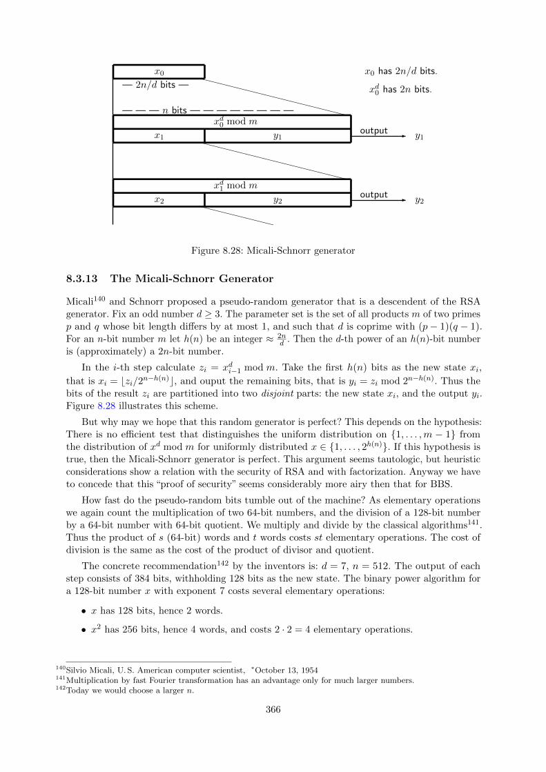
x2 y2
xd1 mod m-output y2
XXXXXXXX
x1 y1
xd0 mod m— — — n bits — — — — — — — —
-output y1XXXXXXXXXXXXXXXX
x0— 2n/d bits —
XXXXXXXXXXXXXXXX
x0 has 2n/d bits.
xd0 has 2n bits.
Figure 8.28: Micali-Schnorr generator
8.3.13 The Micali-Schnorr Generator
Micali140 and Schnorr proposed a pseudo-random generator that is a descendent of the RSAgenerator. Fix an odd number d ≥ 3. The parameter set is the set of all products m of two primesp and q whose bit length differs by at most 1, and such that d is coprime with (p− 1)(q − 1).For an n-bit number m let h(n) be an integer ≈ 2n
d . Then the d-th power of an h(n)-bit numberis (approximately) a 2n-bit number.
In the i-th step calculate zi = xdi−1 mod m. Take the first h(n) bits as the new state xi,
that is xi = bzi/2n−h(n)c, and ouput the remaining bits, that is yi = zi mod 2n−h(n). Thus thebits of the result zi are partitioned into two disjoint parts: the new state xi, and the output yi.Figure 8.28 illustrates this scheme.
But why may we hope that this random generator is perfect? This depends on the hypothesis:There is no efficient test that distinguishes the uniform distribution on {1, . . . ,m − 1} fromthe distribution of xd mod m for uniformly distributed x ∈ {1, . . . , 2h(n)}. If this hypothesis istrue, then the Micali-Schnorr generator is perfect. This argument seems tautologic, but heuristicconsiderations show a relation with the security of RSA and with factorization. Anyway we haveto concede that this “proof of security” seems considerably more airy then that for BBS.
How fast do the pseudo-random bits tumble out of the machine? As elementary operationswe again count the multiplication of two 64-bit numbers, and the division of a 128-bit numberby a 64-bit number with 64-bit quotient. We multiply and divide by the classical algorithms141.Thus the product of s (64-bit) words and t words costs st elementary operations. The cost ofdivision is the same as the cost of the product of divisor and quotient.
The concrete recommendation142 by the inventors is: d = 7, n = 512. The output of eachstep consists of 384 bits, withholding 128 bits as the new state. The binary power algorithm fora 128-bit number x with exponent 7 costs several elementary operations:
• x has 128 bits, hence 2 words.
• x2 has 256 bits, hence 4 words, and costs 2 · 2 = 4 elementary operations.
140Silvio Micali, U. S. American computer scientist, ∗October 13, 1954141Multiplication by fast Fourier transformation has an advantage only for much larger numbers.142Today we would choose a larger n.
366

• x3 has 384 bits, hence 6 words, and costs 2 · 4 = 8 elementary operations.
• x4 has 512 bits, hence 8 words, and costs 4 · 4 = 16 elementary operations.
• x7 has 896 bits, hence 14 words, and costs 6 · 8 = 48 elementary operations.
• x7 mod m has ≤ 512 bits, and likewise costs 6 · 8 = 48 elementary operations.
This makes a total of 124 elementary operations; among them only one reduction mod m (for x7).Our reward consists of 384 pseudo-random bits. Thus we get about 3 bits per elementary operation,or, by the assumptions in Section 8.3.12, about 6 milliards143 bits per second. Compared withthe BBS generator this amounts to a factor of about 1000.
Parallelization increases the speed virtually without limit: The Micali-Schnorr generatorallows complete parallelization. Thus distributing the work among k CPUs brings a profit by thefactor k since the CPUs can work indepedently of each other without need of communication.
8.3.14 Summary and Outlook
Bitstream ciphers need cryptographically secure random generators. These probably exist,however their security—like the security of almost all ciphers—is mathematically not completelyproven.
But implementing a useful bitstream cipher takes more than just a good random generator:
• Message integrity requires additional means such as a combination with a cryptographichash function.
• The operational conditions must prevent the reuse of (parts of) the key stream in areliable way. This means that the key management requires utmost prudence. A possibleapproach144 is using a longtime general key that consists of certain inner parameters ofthe random generator, and use the remaining parameters including the initial state asone-time message key.
In contrast with bitblock ciphers where we have the accepted standard AES (and the outdatedstandard DES) for bitstream ciphers there is no established standard. Closest to standardizationis the eSTREAM portfolio developed in a European project from 2004 until 2008. It recommendsa bunch of several ciphers [Sch03].
Unfortunately several “proprietary” ciphers, mostly bitstream ciphers developed in backrooms by cryptologic amateurs, found their way into security critical applications, relied on“security by obscurity”, but could easily be analyzed by reverse engineering, and teared to shredsby cryptologists. Therefore we finish this chapter with an advice that in an analogous formapplies to all parts of cryptography:
Never trust a random generator whose algorithm is kept secret, or for which noanalysis results are publicly available. Statistical analyses are insufficient as securityproofs, just as little as gargantuan periods, or a gigantic choice of initial states.
143European milliards = American billions144This was a usual approach with the cipher machines of World War II.
367

8.4 Appendix: Boolean Maps in SageMath
8.4.1 What’s in SageMath?
SageMath has several functions for bitblocks and Boolean functions. These are scattered overdifferent modules, use different data types, and have some limitations. We could live with them.Nevertheless in this text we mostly use our own independent (and free) implementation145.
Bitblocks
The SageMath function binary() converts integers into bitstrings. Sample usage:123456789.binary(), result: ’111010110111100110100010101’.
The module sage.crypto.util has the functions ascii_to_bin(), bin_to_ascii(), andascii_integer(). Somewhere else, in sage.crypto.block_cipher.sdes, we find a functionsdes.string_to_list() that converts a bitstring into a list.
Logical Expressions
Functions for logical expressions are in the modules sage.logic.boolformula,sage.sat.converters, sage.sat.solvers, and sage.sat.boolean_polynomials. How-ever these require a mode of thinking different from the approach in this text that is adapted tocryptographic considerations.
Boolean Functions and Maps
For dealing with Boolean functions we may look at the module sage.crypto.boolean_function,and use its functions truth_table(), algebraic_normal_form(), andwalsh_hadamard_transform(), that are implemented as methods of the class BooleanFunction.
For dealing with Boolean maps we have the functions cnf(),linear_approximation_matrix(), and difference_distribution_matrix() as methods ofthe class SBox from the module sage.crypto.mq.sbox.
8.4.2 New SageMath Functions for this Chapter
The SageMath classes and functions defined in the following can be found in the modulebitciphers.sage. They were developed with Python 3.4.1146 under OS X, and tested withSageMath 6.2.
Their usage requires a SageMath installation. In command line mode attach the module viathe SageMath commands
load_attach_path(path=’/my/path’, replace=False)
attach(’bitciphers.sage’)
145This is known as “reinventing the wheel”. Forgive it in view of intended uniformity and consistency. Workingthrough the functions in the SageMath samples should facilitate learning the algorithms. A further aspect: Ourmodules are written in pure Python and may be used without installing SageMath.
146The only relevant difference with Python 2 is the operator // for the division of integers.
368

If you use the worksheet frontend (for a SageMath server), you better copy the single functionseach into an input cell147.
8.4.3 Conversion Routines for Bitblocks
SageMath sample 8.37 Conversion routines for bitblocks
def int2bbl(number,dim):
"""Converts number to bitblock of length dim via base-2
representation."""
n = number # catch input
b = [] # initialize output
for i in range(0,dim):
bit = n % 2 # next base-2 bit
b = [bit] + b # prepend
n = (n - bit)//2
return b
def bbl2int(bbl):
"""Converts bitblock to number via base-2 representation."""
ll = len(bbl)
nn = 0 # initialize output
for i in range(0,ll):
nn = nn + bbl[i]*(2**(ll-1-i)) # build base-2 representation
return nn
147A complete SageMath worksheet containing all samples of this text is available as bitciphers.sws, or in human-readable PDF format as bitciphers_sws.pdf.
369

SageMath sample 8.38 Conversion routines for bitblocks (continued)
def str2bbl(bitstr):
"""Converts bitstring to bitblock."""
ll = len(bitstr)
xbl = []
for k in range(0,ll):
xbl.append(int(bitstr[k]))
return xbl
def bbl2str(bbl):
"""Converts bitblock to bitstring."""
bitstr = ""
for i in range(0,len(bbl)):
bitstr += str(bbl[i])
return bitstr
def txt2bbl(text):
"""Converts ASCII-text to bitblock."""
ll = len(text)
xbl = []
for k in range(0,ll):
n = ord(text[k])
by = int2bbl(n,8)
xbl.extend(by)
return xbl
def bbl2sub(bbl):
"""Converts bitblock to subset."""
ll = len(bbl)
set = []
for i in range(0,ll):
if (bbl[i] == 1):
set.append(i+1)
return set
370

SageMath sample 8.39 Various compositions of bitblocks
def coinc(x,y):
"""Counts coincidences between 2 lists."""
ll = len(x)
assert ll <= len(y), "coinc_Error: Second bitblock too short."
nn = 0
for i in range(0,ll):
if (x[i] == y[i]):
nn += 1
return nn
def binScPr(x,y):
"""Scalar product of two binary vectors (lists) mod 2."""
l = len(x)
assert l == len(y), "binScPr_Error: Blocks have different lengths."
res = 0
for i in range (0,l):
res += x[i] * y[i]
return res %2
def xor(plain,key):
"""Binary addition of bitblocks.
Crops key if longer than plain.
Repeats key if shorter than plain.
"""
lk = len(key)
lp = len(plain)
ciph = []
i = 0
for k in range(0,lp):
cbit = (plain[k] + key[i]) % 2
ciph.append(cbit)
i += 1
if i >= lk:
i = i-lk
return ciph
371

8.4.4 Matsui’s Test
SageMath sample 8.40 Matsui’s test
def Mats_tst(a, b, pc, compl = False):
"""Matsui’s test for linear cryptanalysis"""
NN = len(pc)
results = []
for pair in pc:
ax = binScPr(a,pair[0])
by = binScPr(b,pair[1])
result = (ax + by) % 2
results.append(result)
t_0 = 0
for bb in results:
if bb == 0:
t_0 = t_0 + 1
if 2*t_0 > NN:
if compl:
return [t_0,1,True]
else:
return [t_0,0,True]
elif 2*t_0 < NN:
if compl:
return [t_0,0,True]
else:
return [t_0,1,True]
else:
return [t_0,randint(0,1),False]
372
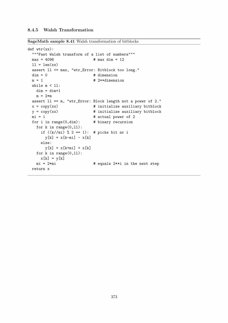
8.4.5 Walsh Transformation
SageMath sample 8.41 Walsh transformation of bitblocks
def wtr(xx):
"""Fast Walsh transform of a list of numbers"""
max = 4096 # max dim = 12
ll = len(xx)
assert ll <= max, "wtr_Error: Bitblock too long."
dim = 0 # dimension
m = 1 # 2**dimension
while m < ll:
dim = dim+1
m = 2*m
assert ll == m, "wtr_Error: Block length not a power of 2."
x = copy(xx) # initialize auxiliary bitblock
y = copy(xx) # initialize auxiliary bitblock
mi = 1 # actual power of 2
for i in range(0,dim): # binary recursion
for k in range(0,ll):
if ((k//mi) % 2 == 1): # picks bit nr i
y[k] = x[k-mi] - x[k]
else:
y[k] = x[k+mi] + x[k]
for k in range(0,ll):
x[k] = y[k]
mi = 2*mi # equals 2**i in the next step
return x
373
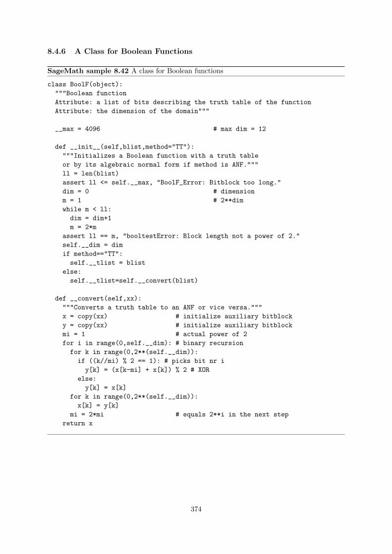
8.4.6 A Class for Boolean Functions
SageMath sample 8.42 A class for Boolean functions
class BoolF(object):
"""Boolean function
Attribute: a list of bits describing the truth table of the function
Attribute: the dimension of the domain"""
__max = 4096 # max dim = 12
def __init__(self,blist,method="TT"):
"""Initializes a Boolean function with a truth table
or by its algebraic normal form if method is ANF."""
ll = len(blist)
assert ll <= self.__max, "BoolF_Error: Bitblock too long."
dim = 0 # dimension
m = 1 # 2**dim
while m < ll:
dim = dim+1
m = 2*m
assert ll == m, "booltestError: Block length not a power of 2."
self.__dim = dim
if method=="TT":
self.__tlist = blist
else:
self.__tlist=self.__convert(blist)
def __convert(self,xx):
"""Converts a truth table to an ANF or vice versa."""
x = copy(xx) # initialize auxiliary bitblock
y = copy(xx) # initialize auxiliary bitblock
mi = 1 # actual power of 2
for i in range(0,self.__dim): # binary recursion
for k in range(0,2**(self.__dim)):
if ((k//mi) % 2 == 1): # picks bit nr i
y[k] = (x[k-mi] + x[k]) % 2 # XOR
else:
y[k] = x[k]
for k in range(0,2**(self.__dim)):
x[k] = y[k]
mi = 2*mi # equals 2**i in the next step
return x
374
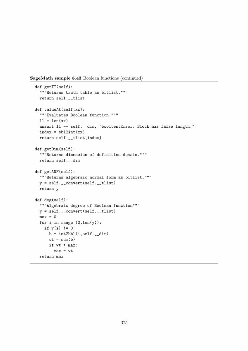
SageMath sample 8.43 Boolean functions (continued)
def getTT(self):
"""Returns truth table as bitlist."""
return self.__tlist
def valueAt(self,xx):
"""Evaluates Boolean function."""
ll = len(xx)
assert ll == self.__dim, "booltestError: Block has false length."
index = bbl2int(xx)
return self.__tlist[index]
def getDim(self):
"""Returns dimension of definition domain."""
return self.__dim
def getANF(self):
"""Returns algebraic normal form as bitlist."""
y = self.__convert(self.__tlist)
return y
def deg(self):
"""Algebraic degree of Boolean function"""
y = self.__convert(self.__tlist)
max = 0
for i in range (0,len(y)):
if y[i] != 0:
b = int2bbl(i,self.__dim)
wt = sum(b)
if wt > max:
max = wt
return max
375

SageMath sample 8.44 Boolean functions: Walsh spectrum and human-readable output
def wspec(self):
"""Calculate Walsh spectrum."""
ff = copy(self.__tlist)
ll = len(ff)
gg = []
for i in range(0,ll):
bit = ff[i]
if (bit):
gg.append(-1)
else:
gg.append(1)
ff = wtr(gg)
return ff
def printTT(self):
"""Prints truth table to stdout."""
for i in range(0,2**(self.__dim)):
bb = int2bbl(i,self.__dim)
print "Value at " + bbl2str(bb) + " is " + repr(self.__tlist[i])
def printANF(self):
"""Prints algebraic normal form to stdout."""
y = self.__convert(self.__tlist)
for i in range(0,2**(self.__dim)):
monom = int2bbl(i,self.__dim)
print "Coefficient at " + bbl2str(monom) + " is " + repr(y[i])
376
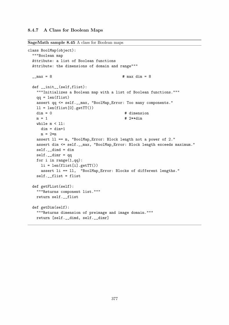
8.4.7 A Class for Boolean Maps
SageMath sample 8.45 A class for Boolean maps
class BoolMap(object):
"""Boolean map
Attribute: a list of Boolean functions
Attribute: the dimensions of domain and range"""
__max = 8 # max dim = 8
def __init__(self,flist):
"""Initializes a Boolean map with a list of Boolean functions."""
qq = len(flist)
assert qq <= self.__max, "BoolMap_Error: Too many components."
ll = len(flist[0].getTT())
dim = 0 # dimension
m = 1 # 2**dim
while m < ll:
dim = dim+1
m = 2*m
assert ll == m, "BoolMap_Error: Block length not a power of 2."
assert dim <= self.__max, "BoolMap_Error: Block length exceeds maximum."
self.__dimd = dim
self.__dimr = qq
for i in range(1,qq):
li = len(flist[i].getTT())
assert li == ll, "BoolMap_Error: Blocks of different lengths."
self.__flist = flist
def getFList(self):
"""Returns component list."""
return self.__flist
def getDim(self):
"""Returns dimension of preimage and image domain."""
return [self.__dimd, self.__dimr]
377
SageMath sample 8.46 Boolean maps (continued)
def getTT(self):
"""Returns truth table as list of bitlists."""
nn = 2**(self.__dimd)
qq = self.__dimr
clist = []
for j in range(0,qq):
clist.append(self.__flist[j].getTT())
transp = []
for j in range(0,nn):
trrow = []
for i in range(0,qq):
trrow.append(clist[i][j])
transp.append(trrow)
return transp
def printTT(self):
"""Prints truth table to stdout."""
nn = 2**(self.__dimd)
qq = self.__dimr
print("Dimensions of truth table:", nn, "by", qq)
clist = []
for j in range(0,qq):
clist.append(self.__flist[j].getTT())
transp = []
for j in range(0,nn):
trrow = []
for i in range(0,qq):
trrow.append(clist[i][j])
transp.append(trrow)
for j in range(0,nn):
bb = int2bbl(j,self.__dimd)
print("Value at", bb, "is", transp[j])
def valueAt(self,xx):
"""Evaluates Boolean map."""
ll = len(xx)
assert ll == self.__dimd, "boolF_Error: Block has false length."
index = bbl2int(xx)
vlist = []
for j in range(0,self.__dimr):
vlist.append(self.__flist[j].getTT()[index])
return vlist
378

SageMath sample 8.47 Boolean maps (continued)
def wspec(self):
"""Calculate Walsh spectrum."""
dd = self.getDim()
tt = self.getTT()
m = 2**(dd[0])
t = 2**(dd[1])
nullv = [0] * t
charF = []
for k in range(0,m):
charF.append(copy(nullv))
for k in range(0,m):
index = bbl2int(tt[k])
charF[k][index] = 1
blist = []
for k in range(0,m):
blist.extend(charF[k])
speclist = wtr(blist)
specmat = []
for k in range(0,m):
specmat.append(speclist[k*t:k*t+t])
return specmat
def linApprTable(self):
"""Calculate the linear approximation table."""
lpr = self.wspec()
dd = self.getDim()
m = 2**(dd[0])
t = 2**(dd[1])
for k in range(0,m):
for i in range(0,t):
lpr[k][i] = (lpr[k][i] + m)//2
return lpr
379
SageMath sample 8.48 Boolean maps: linear profile
def linProf(self, extended=False):
"""Calculate linear profile. If extended is True, also
calculate maximum potential and corresponding linear forms."""
lpr = self.wspec()
dd = self.getDim()
m = 2**(dd[0])
t = 2**(dd[1])
for k in range(0,m):
for i in range(0,t):
lpr[k][i] = lpr[k][i] * lpr[k][i]
if extended:
flatlist = []
for row in lpr:
flatlist.extend(row)
denominator = flatlist.pop(0)
mm = max(flatlist)
ixlist = []
for k in range(0,m):
for i in range(0,t):
if lpr[k][i] == mm:
ixlist.append([k,i])
return [lpr, mm, denominator, ixlist]
else:
return lpr
380

8.4.8 Lucifer and Mini-Lucifer
SageMath sample 8.49 S-boxes and bit permutation of Lucifer
#-------------- Define S0 ----------------------------
f1 = BoolF([1,1,0,1,1,1,1,0,0,0,0,0,1,0,0,1])
f2 = BoolF([1,1,1,0,1,1,0,0,0,1,0,0,0,1,1,0])
f3 = BoolF([0,1,1,1,1,0,1,0,1,1,1,0,0,0,0,0])
f4 = BoolF([0,1,1,0,0,1,1,0,0,0,1,1,1,0,1,0])
S0 = BoolMap([f1,f2,f3,f4])
#-------------- Define S0 inverse -------------------
fi1 = BoolF([0,1,1,1,1,1,1,0,1,1,0,0,0,0,0,0])
fi2 = BoolF([1,0,0,0,1,1,0,0,1,1,0,1,0,1,1,0])
fi3 = BoolF([1,1,0,1,0,1,0,1,1,0,1,1,0,0,0,0])
fi4 = BoolF([1,1,0,0,1,0,1,0,1,0,1,0,0,1,0,1])
S0inv = BoolMap([fi1,fi2,fi3,fi4])
#-------------- Define S1 ----------------------------
g1 = BoolF([0,0,1,1,0,1,0,0,1,1,0,1,0,1,1,0])
g2 = BoolF([1,0,1,0,0,0,0,1,1,1,0,0,1,1,0,1])
g3 = BoolF([1,1,1,0,1,1,0,0,0,0,0,1,1,1,0,0])
g4 = BoolF([1,0,0,1,1,1,0,0,0,1,1,0,0,1,0,1])
S1 = BoolMap([g1,g2,g3,g4])
#-------------- Define S1 inverse -------------------
gi1 = BoolF([0,1,0,0,0,1,1,0,1,0,1,0,1,1,0,1])
gi2 = BoolF([1,0,0,1,1,1,1,0,1,0,0,1,0,0,0,1])
gi3 = BoolF([1,1,0,0,1,1,0,0,1,1,1,0,0,0,1,0])
gi4 = BoolF([0,0,1,0,1,1,0,0,0,1,1,1,0,1,0,1])
S1inv = BoolMap([gi1,gi2,gi3,gi4])
def P(b):
"""Lucifer’s bit permutation"""
pb = [b[2],b[5],b[4],b[0],b[3],b[1],b[7],b[6]]
return pb
381

SageMath sample 8.50 Mini-Lucifer over r rounds
def miniLuc(a,k,r):
"""Mini-Lucifer, encrypts 8-bit a with 16-bit key k over r rounds."""
ll = len(a)
assert ll == 8, "miniLuc_Error: Only blocks of length 8 allowed."
lk = len(k)
assert lk == 16, "miniLuc_Error: Only keys of length 16 allowed."
k0 = k[0:8] # split into subkeys
k1 = k[8:16]
aa = a # round input
# --- begin round
for i in range(0,r): # round number is i+1
if (i % 2 == 0): # select round key
rndkey = k0
else:
rndkey = k1
b = xor(aa,rndkey) # add round key
bleft = b[0:4] # begin substitution
bright = b[4:8]
bbleft = S0.valueAt(bleft)
bbright = S1.valueAt(bright)
bb = bbleft + bbright # end substitution
if (i+1 == r): # omit permutation in last round
aa = bb
else:
aa = P(bb)
# --- end round
if (r % 2 == 0): # add subkey after last round
finkey = k0
else:
finkey = k1
c = xor(aa,finkey)
return c
382

8.4.9 A Class for Linear Feedback Shift Registers
SageMath sample 8.51 A class for linear feedback shift registers
class LFSR(object):
"""Linear Feedback Shift Register
Attributes: the length of the register
a list of bits describing the taps of the register
the state
"""
__max = 1024 # max length
def __init__(self,blist):
"""Initializes a LFSR with a list of taps
and the all 0 state."""
ll = len(blist)
assert ll <= self.__max, "LFSR_Error: Bitblock too long."
self.__length = ll
self.__taplist = blist
self.__state = [0] * ll
def __str__(self):
"""Defines a printable string telling the internals of
the register."""
outstr = "Length: " + str(self.__length)
outstr += " | Taps: " + bbl2str(self.__taplist)
outstr += " | State: " + bbl2str(self.__state)
return outstr
def getLength(self):
"""Returns the length of the LFSR."""
return self.__length
def setState(self,slist):
"""Sets the state."""
sl = len(slist)
assert sl == self.__length, "LFSR_Error: Bitblock has wrong length."
self.__state = slist
383
SageMath sample 8.52 A class for linear feedback shift registers (continued)
def nextBits(self,n):
"""Returns the next n bits as a list and updates the state."""
outlist = []
a = self.__taplist
u = self.__state
for i in range (0,n):
b = binScPr(a,u)
c = u.pop()
u.insert(0,b)
outlist.append(c)
self.__state = u
return outlist
384
Bibliography (Chap BitCiphers)
[Bar09] Bard, Gregory V.: Algebraic Cryptanalysis. Springer, Dordrecht, 2009.
[Bri10] Brickenstein, Michael: Boolean Grobner Bases – Theory, Algorithms and Applications.PhD thesis, TU Kaiserslautern, department of Mathematics, 2010.See also “PolyBoRi – Polynomials over Boolean Rings”, online:http://polybori.sourceforge.net/”.
[CGH+03] Castro, D., M. Giusti, J. Heintz, G. Matera, and L. M. Pardo: The hardness ofpolynomial equation solving. Found. Comput. Math., 3:347–420, 2003.
[CH10] Crama, Yves and Peter L. Hammer (editors): Boolean Models and Methods inMathematics, Computer Science, and Engineering. Cambridge University Press,2010.
[CLO07] Cox, David, John Little, and Donal O’Shea: Ideals, Varieties, and Algorithms.Springer, 3rd edition, 2007.
[CS09] Cusick, Thomas W. and Pantelimon Stanica: Cryptographic Boolean Functions andApplications. Elsevier Academic Press, 2009.
[DR02] Daemen, Joan and Vincent Rijmen: The Design of Rijndael. AES – The AdvancedEncryption Standard. Springer, 2002.
[GJ79] Garey, Michael R. and David S. Johnson: Computers and Intractability. Freeman,1979.
[Gol82] Golomb, Solomon W.: Shift Register Sequences. Aegean Park Press, 1982. RevisedEdition.
[Laz83] Lazard, Daniel: Grobner bases, Gaussian elimination and resolution of systems ofalgebraic equations. In Lecture Notes in Computer Science 162, pages 146–156.Springer, 1983. EUROCAL ’83.
[LV00] Lenstra, Arjen K. and Eric R. Verheul: Selecting Cryptographic Key Sizes. In LectureNotes in Computer Science 558, pages 446–465, 2000. PKC2000.See also “BlueKrypt Cryptographic Key Length Recommendation”, last update 2015,online: http://www.keylength.com/en/2/.
[MS89] Meier, W. and O. Staffelbach: Fast correlation attacks on certain stream ciphers.Journal of Cryptology, 1:159–176, 1989.
[MvOV01] Menezes, Alfred J., Paul C. van Oorschot, and Scott A. Vanstone: Handbook ofApplied Cryptography. Series on Discrete Mathematics and Its Application. CRC
385

Press, 5th edition, 2001, ISBN 0-8493-8523-7. (Errata last update Jan 22, 2014).http://cacr.uwaterloo.ca/hac/,http://www.cacr.math.uwaterloo.ca/hac/.
[Opp11] Oppliger, Rolf: Contemporary Cryptography, Second Edition. Artech House, 2nd edi-tion, 2011. http://books.esecurity.ch/cryptography2e.html.
[Pom08] Pommerening, Klaus: Linearitatsmaße fur Boolesche Abbildungen, 2008. Manuskript,30. Mai 2000. Letzte Revision 4. Juli 2008.English equivalent: Fourier Analysis of Boolean Maps – A Tutorial.http://www.staff.uni-mainz.de/pommeren/Kryptologie/Bitblock/A_Nonlin
/nonlin.pdf.
[Pom14] Pommerening, Klaus: Fourier Analysis of Boolean Maps – A Tutorial, 2014.Manuscript: May 30, 2000. Last revision August 11, 2014.German aequivalent: Linearitatsmaße fur Boolesche Abbildungen.http://www.staff.uni-mainz.de/pommeren/Cryptology/Bitblock/Fourier/Fo
urier.pdf.
[Pom16] Pommerening, Klaus: Cryptanalysis of nonlinear shift registers. Cryptologia, 30,2016.http://www.tandfonline.com/doi/abs/10.1080/01611194.2015.1055385.
[PP09] Paar, Christof and Jan Pelzl: Understanding Cryptography – A Textbook for Studentsand Practioners. Springer, 2009.
[Sch03] Schmeh, Klaus: Cryptography and Public Key Infrastructure on the Internet. JohnWiley, 2003. In German, the 6th edition was published in 2016.
[Sch16] Schmeh, Klaus: Kryptographie – Verfahren, Protokolle, Infrastrukturen. dpunkt.verlag,6th edition, 2016. Sehr gut lesbares, aktuelles und umfangreiches Buch uber Kryptogra-phie. Geht auch auf praktische Probleme (wie Standardisierung oder real existierendeSoftware) ein.
[Seg04] Segers, A. J. M.: Algebraic Attacks from a Grobner Basis Perspective. Master’s thesis,Technische Universiteit Eindhoven, 2004.http://www.win.tue.nl/~henkvt/images/ReportSegersGB2-11-04.pdf.
[SL07] Stamp, Mark and Richard M. Low: Applied Cryptanalysis: Breaking Ciphers in theReal World. Wiley-IEEE Press, 2007.http://cs.sjsu.edu/faculty/stamp/crypto/.
[Sti06] Stinson, Douglas R.: Cryptography – Theory and Practice. Chapman & Hall/CRC,3rd edition, 2006.
[vzGG99] Gathen, Joachim von zur and Jurgen Gerhard: Modern Computer Algebra. CambridgeUniversity Press, 1999.
All links have been confirmed at July 15, 2016.
386
Chapter 9
Homomorphic Ciphers
(Martin Franz, Jan 2013)
9.1 Introduction
Homomorphic ciphers are public-key cryptosystems with special properties. They allow perform-ing certain arithmetic operations on encrypted ciphertexts, without knowing the correspondingplaintexts and without having to decrypt the ciphertexts first. These special properties haveled to a huge amount of applications for homomorphic ciphers, e.g. in the domain of cloudcomputing. A very famous and relatively new cryptosystem with homomorphic properties is thePaillier cryptosystem. But also some of the older and well established cryptosystems, such asElGamal or RSA, have homomorphic properties.
9.2 Origin of the term “homomorphic”
We first clarify the meaning and the origin of the term“homomorphic”. This term in cryptographyis derived from its counterpart in mathematics: in mathematics, a homomorphism is a structure-preserving map between two algebraic structures. In the common sense this means, that ahomomorphism f : X → Y maps the structure of X to the structure of Y . Using an example,this can be easily illustrated: Let (X,+) and (Y, ∗) two algebraic groups with group operations+ and ∗, respectively. A homomorphism f : X → Y maps any given x ∈ X to a value y ∈ Y , ina way that it holds:
f(x1 + x2) = f(x1) ∗ f(x2)
for any two x1, x2 in X. This means, that for any two values x1, x2 it does not matter whetherwe first compute their sum (group operation of X) and then apply f (this is the left side of theabove given equation); or, whether we first apply f to the values x1, x2, and then compute theirproduct in Y , thus apply the group operation of Y . Please note that the operations + and ∗were chosen here only as an example, they always depend on the algebraic group they belongto. Naturally, the same relation holds for homomorphisms between groups with the same groupoperation.
Example: Let X = Z be the set of integer values. The set Z together with the additionoperation forms an algebraic group G1 = (Z,+). Similarly, the real values R without the valuezero together with the multiplication operation form a group G2 = (R\{0}, ∗). The functionf : Z→R\{0}, z→ez is a homomorphism, since for all z1, z2 ∈ Z it holds: f(z1 + z2) = e(z1+z2) =
387

f(z1) ∗ f(z2). On the contrary, f : Z→ R\{0}, z → z2 is an example for a function which is nota homomorphism.
9.3 Decryption function is a homomorphism
In the remainder of this chapter we will consider public-key cryptosystems with a special property,namely that its decryption function is a homomorphism. A public-key cryptosystem with thisproperty will be called homomorphic.
Let us for now assume, the above described homomorphism f is the decryption function ofa known cryptosystem. This means that we can perform certain algebraic operations in theciphertext space, knowing which effects this will have on their plaintexts. Following the abovegiven example:
Y corresponds to the set of cipher texts, X is the set of plaintexts. For two plaintexts x1, x2with corresponding ciphertexts y1, y2 it holds:
f(y1 ∗ y2) = f(y1) + f(y2) = x1 + x2
This equation can be interpreted as follows: If we multiply two ciphertexts y1, y2 with each otherand subsequently decrypt their product, then we will obtain the sum of the originally encryptedvalues x1 and x2. Everybody can – without knowledge of the plaintexts, without having todecrypt and even without knowing the private decryption key – compute a product of the twociphertexts and knows that upon decryption the owner of the private key will obtain the sum ofthe two originally encrypted plaintexts.
9.4 Examples of homomorphic ciphers
9.4.1 Paillier cryptosystem
The most famous cryptosystem with homomorphic properties is the one by Paillier [Pai99]. Firstwe will see how the Paillier key generation process works. After that, we will show that thePaillier cryptosystem indeed has homomorphic properties.
9.4.1.1 Key generation
First, we generate two random prime numbers p, q in a way that their product n = pq forms avalid RSA modulus. As for common RSA, the value n should have a bit length of at least 1024bits.
Using the prime values p and q, we can compute the value λ = lcm(p− 1, q − 1). lcm heredenotes the least common multiple. The RSA modulus n will now be the public key, while theprivate key is the value λ.
9.4.1.2 Encryption
Let m be the message which will be encrypted, where m is taken from the plaintext space Zn. Foreach encryption, we first choose a random element r from the plaintext space Zn. Subsequently,using the public key, we compute the ciphertext n as:
c = E(m, r) = (n+ 1)m ∗ rn mod n2
388

9.4.1.3 Decryption
Given the private key λ and a ciphertext c ∈ Z∗n2 , we first compute S = cλ mod n2 and
subsequently T = φ(n)(−1) mod n2, where φ denotes the Euler function.
Finally, we compute the plaintext m = D(c) = (S − 1)/n ∗ T mod n.
9.4.1.4 Homomorphic property
We will now show that the Paillier cryptosystem has the homomorphic property as describedabove. For this, we will use E to denote the encryption and D to denote the decryption functionof the Paillier cryptosystem. For simplicity, we set g := n+ 1. For any two plaintexts m1,m2
and random values r1, r2 we obtain ciphertexts c1, c2 as
c1 = gm1 ∗ r1n mod n2 and c2 = gm2 ∗ r2n mod n2,
respectively. Now it is easy to see that for the product c3 = c1 ∗ c2 it holds
c3 = (gm1 ∗r1n mod n2)∗ (gm2 ∗r2n mod n2) = gm1+m2 ∗ (r1 ∗r2)n mod n2 = E(m1 +m2, r1 ∗r2)
Thus, the product of two given ciphertexts is in fact a valid ciphertext, namely the encryptionof the sum of the originally encrypted messages. Now it is straightforward to see that thedecryption function is a homomorphism. Given two plaintexts m1,m2 it holds
D(E(m1, r1) ∗ E(m2, r2)) = D(E(m1 +m2, r1r2)) = m1 +m2 = D(E(m1, r1)) +D(E(m2, r2))
9.4.2 Other cryptosystems
Also older public-key cryptosystems can have homomorphic properties. Both the ElGamalcryptosystem and RSA constitute famous examples. We will show their homomorphic propertiesby means of some easy examples.
9.4.2.1 RSA
Let (e, n) be the public RSA key (e the public encryption exponent, n the RSA modulus). For anytwo messages m1,m2 we obtain encryptions c1 = m1
e mod n and c2 = m2e mod n. Now for the
product of these two encryptions it holds: c1 ∗ c2 = m1e ∗m2
e mod n = (m1 ∗m2)e mod n. Thus,we obtain an encryption of the product of the two messages m1 and m2. As it is straightforwardto see, this property holds for any two plaintexts m1,m2 and similar as for Paillier, the decryptionfunction is a homomorphism. As we have seen here, RSA is an example for a homomorphism,where both groups have the same group operation.
9.4.2.2 ElGamal
Similar to RSA we can also show the homomorphic properties of the ElGamal cryptosystem.Let (p, g,K) the public key while the private key is k (thus, it holds gk mod p = K). For anytwo messages m1,m2 and random values r, s we obtain encryptions (R, c1) = (Kr mod p,m1 ∗gr mod p) and (S, c2) = (Ks mod p,m2 ∗ gs mod p). As for RSA, we verify that their product(R ∗ S, c1 ∗ c2) is an encryption of m1 ∗m2. Again it is straightforward to see that the decryptionfunction is a homomorphism.
389
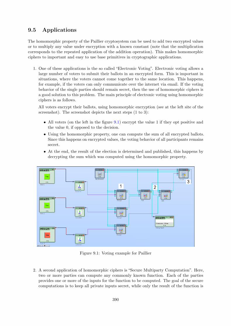
9.5 Applications
The homomorphic property of the Paillier cryptosystem can be used to add two encrypted valuesor to multiply any value under encryption with a known constant (note that the multiplicationcorresponds to the repeated application of the addition operation). This makes homomorphicciphers to important and easy to use base primitives in cryptographic applications.
1. One of these applications is the so called “Electronic Voting”. Electronic voting allows alarge number of voters to submit their ballots in an encrypted form. This is important insituations, where the voters cannot come together to the same location. This happens,for example, if the voters can only communicate over the internet via email. If the votingbehavior of the single parties should remain secret, then the use of homomorphic ciphers isa good solution to this problem. The main principle of electronic voting using homomorphicciphers is as follows.
All voters encrypt their ballots, using homomorphic encryption (see at the left site of thescreenshot). The screenshot depicts the next steps (1 to 3):
• All voters (on the left in the figure 9.1) encrypt the value 1 if they opt positive andthe value 0, if opposed to the decision.
• Using the homomorphic property, one can compute the sum of all encrypted ballots.Since this happens on encrypted values, the voting behavior of all participants remainssecret.
• At the end, the result of the election is determined and published, this happens bydecrypting the sum which was computed using the homomorphic property.
Figure 9.1: Voting example for Paillier
2. A second application of homomorphic ciphers is “Secure Multiparty Computation”. Here,two or more parties can compute any commonly known function. Each of the partiesprovides one or more of the inputs for the function to be computed. The goal of the securecomputations is to keep all private inputs secret, while only the result of the function is
390

revealed. The use of homomorphic encryption helps to perform these computations onencrypted data. However, since the Paillier encryption only allows to compute additions ofencrypted values (and, e.g. no multiplications can be performed), a number of additionalmethods and techniques have to be applied. The Wikipedia page [Wikb] offers a great startfor reading more about this topic and more advanced techniques for Secure MultipartyComputation.
3. Furthermore it is expected, that homomorphic encryption will provide great advantages inthe areas of “Cloud Computing”. Using so called “fully-homomorphic encryption” [Wika] itwill be possible to run large applications on external servers only on encrypted data. Forthis, necessarily one needs to be able to perform both arithmetic operations, the additionand the multiplication, on encrypted data (in contrast to Paillier encryption, which onlyallows performing additions). Such a crypto system was first presented in 2009 [Gen09].
9.6 Homomorphic ciphers in CrypTool
9.6.1 CrypTool 2
In CrypTool 2 you will find an implementation of the Paillier cryptosystem. Among the availablecomponents, there are components for key generation (Paillier Key Generator), an examplefor encryption and decryption with Paillier (called Paillier Text), as well as examples whichillustrate the homomorphic properties of the cryptosystem (Paillier Addition, Paillier Blindingand Paillier Voting).
Figure 9.2: Paillier cryptosystem in CrypTool 2 (CT2)
391

9.6.2 JCrypTool
In JCrypTool there is an implementation (see Figure 9.3), which visualizes the homomorphicproperties of various cryptosystem. For RSA and Paillier it shows, that multiplications, forRSA, and additions for Paillier, respectively, can be performed on encrypted values. For thefully-homomorphic cryptosystem by Gentry it is possible to perform both multiplications, aswell as additions on encrypted values.
Figure 9.3: Visualization of homomorphic properties in JCrypTool (JCT)
392

Bibliography (Chap HE)
[Gen09] Gentry, Craig: Fully Homomorphic Encryption Using Ideal Lattices. In 41st ACMSymposium on Theory of Computing (STOC), 2009.
[Pai99] Paillier, Pascal: Public-Key Cryptosystems Based on Composite Degree ResiduosityClasses. In Advances in Cryptology – EUROCRYPT’99, 1999.
[Wika] Wikipedia: Homomorphic Encryption & Homomorphismus.https://en.wikipedia.org/wiki/Homomorphic_encryption,https://de.wikipedia.org/wiki/Homomorphismus.
[Wikb] Wikipedia: Secure Multiparty Computation.http://en.wikipedia.org/wiki/Secure_multi-party_computation.
All links have been confirmed at July 15, 2016.
393

Chapter 10
Survey on Current AcademicResults for Solving DiscreteLogarithms and for Factoring – AndHow to React in Practice
(Antoine Joux, Arjen Lenstra, & Alexander May; Apr 2014)
Abstract: Recent algorithmic developments for solving discrete logarithms in finite fields ofsmall characteristic led to some uncertainty among cryptographic users fueled by the mediaabout the impact for the security of currently deployed cryptographic schemes (see for instancethe discussion in [PRSS13] using the catchword “cryptocalypse”). This survey provides a broaderpicture about the currently best algorithms for computing discrete logarithms in various groupsand about the status of the factorization problem. Our goal is to clarify what currently canbe done algorithmically and what cannot be done without further major breakthroughs. Inparticular, we currently do not see a way how to extend the current algorithmic progress forfinite fields of small characteristic to either the case of large characteristic finite fields or to theinteger factorization problem.
394

10.1 Generic Algorithms for the Discrete Logarithm Problemin any Group
Management Summary: The hardiness of the Discrete Logarithm Problem dependson the group over which it is defined. In this chapter we review cryptanalyticalalgorithms that work for any group. From a cryptographic point of view it is de-sirable to identify groups for which one is unable to find better algorithms. Onecandidate for these groups are elliptic curve groups.
In this chapter, we describe general cryptanalytical algorithms that apply for any finiteabelian group. That means, any group used in cryptography – e.g. multiplicative groups offinite fields or of elliptic curves – are susceptible to this kind of algorithms. We will see that wecan always compute a discrete logarithm in a group of order n in O(
√n) steps by Pollard’s Rho
Method. This in turn means that for achieving a security level of 2k one has to choose a groupof order at least 22k. E.g. for achieving a security level of 80 bits, one has to choose a group oforder at least 160 bits. This explains why in practice we usually take elliptic curve groups withat least 160 bit order.
Moreover, let G be a group of order n and let n = pe11 · . . . · pe`` be the prime factorization of n.
Then we will see that discrete logarithms in G can be computed in time O(e1√p1 + . . .+ e`
√p`).
Notice that this bound is equal to Pollard’s bound O(√n) if and only if n is a prime. Otherwise,
the complexity of computing the discrete logarithm is mainly determined by the size of thelargest prime divisor of its group order. This explains why e.g. Schnorr/DSA signatures areimplemented in groups which contain by construction a prime factor of size at least 160 bits.This also explains why usually elliptic curve groups have prime order or order containing only avery small smooth co-factor.
10.1.1 Pollard Rho Method
Let G be a finite abelian group. Let g be a generator of some large subgroup G′ = {g, g2, . . . , gn} ⊆G (e.g. g could generate G itself). Let y = gx. Then the discrete logarithm problem is to findon input g and y the output x mod n. We write x = dlogg(y).
Pollard’s Rho method tries to generate elements gaiybi ∈ G′ with ai, bi ∈ N in a pseudo-random but deterministic fashion. Let us assume for simplicity that we generate random elementsfrom the n elements in G′. Then by the birthday paradox, we expect to find after only O(
√n)
steps two elements which are identical. In our case, this means that
gaiybi = gajybj .
This can be rewritten as gai−ajbj−bi = y. This in turn implies that we can recover our discrete
logarithm as x ≡ ai−ajbj−bi mod n.
Hence, with Pollard’s Rho method one can compute discrete logarithms in any finite abeliangroup of order n in O(
√n) steps. By using so-called cycle-finding techniques, one can also show
that Pollard’s Rho Method can be implemented within constant space.
Moreover, it is also possible to improve the efficiency of square root algorithms when multiplediscrete logarithms in the same group are desired: When computing L distinct logarithms, onecan reduce the global cost from O(L
√n) to O(
√Ln) [FJM14].
395

10.1.2 Silver-Pohlig-Hellman Algorithm
As before let y = gx for a generator g of order n. We have to compute the discrete logarithmx mod n. Moreover, let n = pe11 · . . . · p
e`` be the prime factorization of n. Then by the Chinese
Remainder Theorem x mod n is uniquely defined by the system of congruences
x ≡ x1 mod pe11...
x ≡ x` mod pe`` .
(10.1)
The algorithm of Silver-Pohlig-Hellman computes all discrete logarithms xi mod pi in thesubgroups of order pi in O(
√pi) steps by using Pollard’s Rho method. Then it is quite easy to
find a logarithm modulo the prime power xi mod peii by a Hensel lifting process that performs eicalls to the discrete logarithm procedure modulo pi. In a Hensel lifting process, we start by asolution xi mod pi, and then consecutively compute xi mod p2i , xi mod p3i , etc. until xi mod peii(see [May13] for Hensel’s formula).
Finally, one computes the desired discrete logarithm x mod n from the above system ofequations (10.1) by Chinese Remaindering. In total, the running time is mainly determinedby computing xi mod pi for the largest prime factor pi. That is, the running time is roughlyO(maxi{
√pi}).
10.1.3 How to Measure Running Times
Throughout this survey, we want to measure the running time of analysis algorithms for discretelogarithms as a function of the bit-size of n. Note that any integer n can be written with(roughly) log n bits, where log is to base 2. Thus, the bit-size of n is log n.
For expressing our running times we use the notation Ln[b, c] = expc·(lnn)b(ln lnn)1−b for
constants b ∈ [0, 1] and c > 0. Notice that Ln[1, c] = ec·lnn = nc is a function that is forconstant c a polynomial in n. Therefore, we say that Ln[1, c] is polynomial in n. Also notice thatLn[1, c] = nc = (2c)log2 n is a function that is exponential in log n. Therefore, we say that Ln[1, c]is exponential in the bit-size logn of n. So our Pollard Rho algorithm achieves exponentialrunning time L[1, 12 ].
On the other end, Ln[0, c] = ec·ln lnn = (lnn)c is polynomial in the bit-size of n. Notice thatthe first parameter b is more important for the running time than the second parameter c, sinceb interpolates between polynomial and exponential running time. We shortly denote Ln[b] if wedo not want to specify the constant c.
Some of the most important algorithms that we discuss in the subsequent sections achieve arunning time of Ln[12 + o(1)] or Ln[13 + o(1)] (where the o(1)-part vanishes for n→∞), which isa function that grows faster than any polynomial but slower than exponential. For cryptographicschemes, such attacks are completely acceptable, since the desired security level can be easilyachieved by a moderate adjustment of the key sizes.
However, the recent algorithm of Joux et al. for computing discrete logarithms in finite fieldsof small characteristic achieves a running time of Ln[o(1)], where o(1) converges to 0 for n→∞.This means that these algorithms are quasi polynomial time, and the underlying fields are nolonger acceptable for cryptographic applications. A finite field Fpn has small characteristic if p issmall, i.e. the base field Fp is small and its extension degree n is usually large. In the recentalgorithms we need a small p, since the algorithms enumerate over all p elements in the basefield Fp.
396

10.1.4 Insecurity in the Presence of Quantum Computers
In 1995, Shor published an algorithm for computing discrete logarithms and factorizations ona quantum computer. He showed that computing discrete logarithms in any group of order ncan be done in polynomial time which is almost O(logn2). The same running time holds forcomputing the factorization of an integer n. This running time is not only polynomial, but theattacks are even more efficient than the cryptographic schemes themselves! This in turn meansthat the problem cannot be fixed by just adjusting key sizes.
Thus, if we face the development of large-scale quantum computers in the next decades, thenall classical dlog- and factoring-based cryptography has to be replaced. However, one shouldstress that the construction of large quantum computers with many qubits appears to be waymore difficult than its classical counterpart, since most small quantum systems do not scale welland face decoherence problems.
Recommendation: It seems hard to predict the developments in constructing quantum com-puters. But experts in quantum physics currently do not see any mayor obstacle that wouldhinder the development of large quantum computers in the long term. It seems crucial tokeep track of current progress in this area, and to have some alternative quantum-resistantcryptosystems ready to enroll within the next 15 years.
References and further reading: We recommend to read the books of Menezes, van Oorschotand Vanstone [MvOV01], Joux [Jou09] and Galbraith [Gal12] for a survey of cryptanalytictechniques. An introductory course in cryptanalysis is provided by May’s lecture notes oncryptanalysis [May08, May12](German). An introduction to quantum algorithms can be foundin the books of Homeister [Hom07](German) and Mermin [Mer08].
The algorithms of this section were originally presented in the superb works of Pollard [Pol75,Pol00] and Shor [Sho94]. Generic algorithms for multiple dlogs have recently been studiedin [FJM14].
397

10.2 Best Algorithms for Prime Fields Fp
Management Summary: Prime fields Fp are – besides Elliptic Curves – the standardgroup for the discrete logarithm problem. There has been no significant algorith-mic progress for this groups in the last 20 years. They are still a good choice forcryptography.
In Chapter 10.1, we learned that in any finite abelian group of order n, we can determinediscrete logarithms in O(
√n) steps. Notice that both the Pollard Rho Method as well as the
Silver-Pohlig-Hellman algorithm from Chapter 10.1 used no other property of representations ofgroup elements than their uniqueness. In these methods, one simply computes group elements bygroup operations and checks for equality of elements. Algorithms of this type are called genericin the literature.
It is known that generic algorithms cannot compute discrete logarithms in time better thanthe Silver-Pohlig-Hellman algorithm [Sho97]. Thus, the algorithms of Chapter 10.1 can beconsidered optimal if no further information about the group elements is used.
However, when we specify our group G as the multiplicative group of the finite field Fp, wherep is a prime, we can actually exploit the representation of group elements. Natural representativesof Fp are the integer 0, . . . , p− 1. Thus, we can e.g. use the prime factorization of these integers.This is done in the so-called Index Calculus type discrete logarithm algorithms. This type ofalgorithm currently forms the class with the best running times for discrete logarithm over primefields, prime extensions (Chapter 10.3) and for the factorization problem (Chapter 10.4).
We will now illustrate an Index Calculus algorithm with a very easy example.
10.2.1 An Introduction to Index Calculus Algorithms
An Index Calculus algorithm consists of three basic steps.
Factor base: Definition of a factor base F = {f1, . . . , fk}. We want to express group elementsas powers of elements of the factor base.
Relation finding: Find elements zi := gxi ∈ G for some integer xi that can be written in thefactor base, that is
gxi =
k∏j=1
feijj .
When we write this equality to the base g, we obtain a relation
xi ≡k∑j=1
eijdlogg(fj) mod n,
where n is the order of g. A relation is a linear equation in the k unknowns
dlogg(f1), . . . ,dlogg(fk)
. Once we have k linear independent relations of this type, we can compute these unknownsby linear algebra. This means we actually first compute all discrete logarithms of thefactor base elements before we compute our desired individual logarithm of y.
398

Dlog computation: Express ygr = gx+r =∏kj=1 f
ejj in the factor base for some integer r. This
gives us another relation
x+ r ≡k∑j=1
ejdlogg(fj) mod n,
which can be easily solved in the only unknown x = dloggy.
Let us provide an easy example for an Index Calculus algorithm that computes x = dlog2(5)in F∗11. Since 2 generates the multiplicative group F∗11, the order of 2 is 10.
Factor base: Define F = {−1, 2}.
Relation finding: 21 = (−1)021 gives us a first trivial relation
1 ≡ 0 · dlog2(−1) + 1 · dlog2(2) mod 10.
If we compute 26 = 64 ≡ −2 mod 11 we obtain a second relation
6 ≡ 1 · dlog2(−1) + 1 · dlog2(2) mod 10.
Therefore, we can solve the system of linear equations(0 11 1
)·(
dlog2(−1)dlog2(2)
)≡(
16
)mod 10.
We obtain as the unique solution dlog2(−1) ≡ 5 and dlog2(2) ≡ 1.
Dlog computation: Since 5 · 21 = 10 ≡ −1 mod 11 we obtain that
x+ 1 ≡ 1 · dlog(−1) + 0 · dlog(2) mod 10.
This leads to the solution x ≡ 4 mod 10.
Runtime: Choosing a large factor base makes it easier to find relations, since it increases thelikelihood that a certain number splits in the factor base. On the other hand, for a large factorbase we have to find more relations in order to compute the dlogs of all factor base elements.An optimization of this tradeoff leads to a running time of Lp[
12 ] for the relation finding step
and also Lp[12 ] for performing the individual discrete logarithm computation in step 3.
Let us briefly discuss the advantages and disadvantages of the above simple Index Calculusalgorithm from a cryptanalyst’s point of view.
Advantages:
• For gxi =∏kj=1 f
eijj it is trivial to compute the discrete logarithm on the left hand size.
Disadvantages:
• We need to factor relatively large numbers gxi over the integers. One can show that thisintrinsically leads to a running time of Lp[
12 ], and there is no hope to get below the constant
12 .
• We need to compute all discrete logarithms of the factor base elements. This is inherentto all Index Calculus algorithms.
We will eliminate the first disadvantage by allowing factorizations over number fields. Thesecond disadvantage is eliminated by choosing a factor base that allows for very efficient discretelogarithm computations of its elements.
399

10.2.2 The Number Field Sieve for Calculating the Dlog1
A number field Q[α] is a k-dimensional vector space over Q and can be obtained by adjoining aroot α of some irreducible degree-k polynomial f to Q. This means we can write every elementof Q[α] as a0 + a1α+ . . . ak−1α
k−1 with ai ∈ Q. If we restrict the ai to integers we are in thering Z[α].
The number field sieve is also an index calculus algorithm. Compared to the previous approachit has the advantage to involve smaller numbers. This is done by choosing a specific representationof the prime field Fp, which is implicitly defined as a finite field where two polynomials of smalldegree with small coefficients possess a common root. There are several methods that allowto construct such polynomials with a common root modulo p. In particular, for primes of aspecial form, i.e. with a sparse representation, it is possible to construct polynomials which aremuch better than in the general case. One typical construction that works well is to choosea number m and write p in basis m as
∑ti=0 aim
i. We then find that f1(X) = X −m andf2(X) =
∑ti=0 aim
i have m as a common root modulo p.
Equipped with two polynomials f1 and f2 of this form, with m as their common root modulop, we obtain the following commutative diagram:
Z[X]
Q[X]/(f1(X)) Q[X]/(f2(X))
Fp
X 7→mX 7→m
Let r1, r2 be roots of f1, f2, respectively. Then we are working with the number fieldsQ[r1] ' Q[X]/(f1(X)) and Q[r2] ' Q[X]/(f2(X)).
Factor base: Consists of small-norm prime elements in both number fields.
Relation finding: The basic principle of the number field sieve consists of sending elements ofthe form a+ bX to both sides of the diagram and to write a relation when both sides factorinto the factor base. Technically, this is quite challenging, because we need to introduceseveral tools to account for the fact that the left and right sides are not necessarily uniquefactorization domains. As a consequence, we need to factor elements into ideals and takecare of the obstructions that arise from the class groups and unit groups. This proceduregives us the discrete logarithms of the factor base elements
Discrete log computation: Express the desired logarithm as a linear combination of thefactor base elements.
Runtime: The Number Field Sieve is the most efficient currently known algorithm for the largecharacteristic discrete logarithm problem. In the general case – which means that p is not of a
special form, e.g. close to a prime power – its complexity is Lp[13 ,(649
)1/3].
References and further reading: For an introduction to Index Calculus and the involvedmathematical tools see May’s lecture notes on number theory [May13](german) and the number
1When calculating the dlog there is only the term number field sieve and no distinction between general vs.special. This is in the opposite to the number field sieve for factorization in section 10.4.1.
400

theory book by Muller-Stach, Piontkowski [MSP11]. For gaining a deep understanding of theNumber Field Sieve, one has to study the book of Lenstra, Lenstra [LL93] that contains alloriginal works that led to the development of the Number Field Sieve algorithm in the late 80sand early 90s.
As a good start for understanding the Number Field Sieve, we recommend to first study itspredecessors that are described in the original works of Adleman [Adl79], Coppersmith [COS86]and Pomerance [Pom84, Pom96].
401

10.3 Best Known Algorithms for Extension Fields Fpn and Re-cent Advances
Management Summary: The groups over extension fields are attacked by the newalgorithms of Joux et al. Before the invention of these attacks, the security ofextension field groups appeared to be similar to the prime order groups from thelast chapter. The new attacks render these groups completely insecure. However,the new attacks do not affect the security of prime order groups.
We will first discuss the formerly best algorithm from 2006 due to Joux and Lercier thatachieves a running time of Ln[13 ]. We will then describe the recent developments that led to thedramatic improvement in the running time down to Ln[o(1)], which is quasi polynomial time.
10.3.1 The Joux-Lercier Function Field Sieve (FFS)
Any finite field Fpn can be represented by a polynomial ring Fp[x]/f(x), where f(x) is anirreducible polynomial over Fp with degree n. Thus, any element in Fpn can be represented by aunivariate polynomial with coefficients in Fp of degree less than n. Addition of two elements isthe usual addition of polynomials, where the coefficients are reduced modulo p. Multiplicationof two elements is the usual multiplication of polynomials, where the result is reduced modulof(x) in order to again achieve a polynomial of degree less than n.
It is important to notice that the description length of an element is nO(log p). Thus, apolynomial time algorithm achieves a running time which is polynomial in n and log p. We willalso consider fields of small characteristic p, where p is constant. Then polynomial running timemeans polynomial in n.
It is known that for any p there are always polynomials f(x) of degree n that are irreducibleover Fp. Usually, there are many of these polynomials, which in turn means that we obtaindifferent representations of a finite field when choosing different polynomials f(x). However, it isalso known that all of these representations are isomorphic, and the isomorphisms are efficientlycomputable.
This fact is used in the algorithm of Joux and Lercier, who exploit different representationsFp[x]/f(x) and Fp[y]/g(y) of the same field. This is illustrated in the following commutativediagram.
Fp[X,Y ]
Fp[X] Fp[Y ]
Fpn
Y 7→f(X)
X 7→g(Y )
X 7→xY 7→y
Factor base: We choose all degree-1 polynomials x− a and y − b from Fp[x] ∪ Fp[y]. Thus, thefactor base has size 2p.
Relation finding: On both sides, that is for polynomials h from Fp[x]/f(x) and from Fp[y]/g(y),we try to factor into the linear factors from the factor base. This can be done by an easy
402

gcd computation gcd(h, xp − x) in time O(p) for each polynomial. It can be shown thatthe number of polynomials that have to be tested is bounded by Lpn [13 ].
Discrete log computation: This step is done by writing a polynomial as a linear combinationof polynomials of smaller degree and by repeating recursively, until degree-1 is found. Thisrecursion is called a (degree) decent and requires running time Lpn [13 ], just like the relationfinding step.
10.3.2 Recent Improvements for the Function Field Sieve
The first recent improvement upon the Joux-Lercier FFS was presented at Eurocrypt 2013 byJoux, who showed that it is possible to drastically lower the complexity of finding relationsby replacing the classical sieving approach with a new technique based on a linear change ofvariables called pinpointing.
At the Crypto Conference 2013, Gologlu, Granger, McGuire, and Zumbragel presentedanother approach, related to pinpointing that works very efficiently with a characteristic 2subfield. Their paper was considered so important by the cryptographic community that theyreceived the best paper award.
The new results hold for finite fields Fqn of characteristic two, i.e. q = 2`. Notice that we usethe standard convention that denotes primes by p and prime powers by q = p`. For these fieldsFqn the relation finding step in the Joux-Lercier algorithm simplifies, since one can constructpolynomials that split with a higher probability than generic polynomials of the same degree.
Let us give a high-level description of the ideas of their improvement.
Factor base: All degree-1 polynomials as in the Joux-Lercier algorithm.
Relation finding: Gologlu, Granger, McGuire, and Zumbragel show that one can constructa special type of polynomials over Fq[x] – the so-called Bluher polynomials – that byconstruction split over Fq[x]. So similar to our simple version of Index Calculus for integersin Section 10.2.1, we obtain one side of the equation for free. The cost for splitting thepolynomials in Fq[y] is roughly O(q) and the cost for finding the discrete logarithms ofthe factor base elements is roughly O(n · q2). We will explain below why this gives us thediscrete logarithms of the factor base in polynomial time for properly chosen parameters.
Discrete log computation: The individual discrete logarithm computation is similar to theJoux-Lercier algorithm.
Runtime: We are computing in a field Fqn , where q = 2`. Hence, a polynomial time algorithmwould require running time polynomial in the parameters n and log q. However, the relationfinding above takes time O(n · q2), which is polynomial in n but exponential in log q. So actuallythe algorithm performs very poorly with respect to the size of the base field Fq = F2` .
The trick to work around this is to decrease the size of the base q to q′ while slightly increasingthe extension degree n to n′. Our goal is that the new base field size q′ roughly equals thenew extension degree n′, that is q′ ≈ n′. In this case, we again obtain a running time which ispolynomial in n′ and q′, but now q′ is also polynomially bounded by n′. So in total, for step 2our running time is in total polynomially bounded by n′.
Let us give a simple example of how this can be done for concrete parameters. Assumethat we wish to compute a discrete logarithm in F(2100)100 . Then we would lower the base field
403
to q′ = 210 and at the same time increase the extension degree to n′ = 1000, i.e. compute inF(210)1000 . Notice that this can always be done by using the efficiently computable isomorphismsbetween finite fields of the same cardinality.
Warning: One might be tempted to bypass the above with the selection of exponents that donot split appropriately, i.e. by choosing F2p with prime p. However, we can always embed ourfinite field in some larger field – as well as the respective discrete logarithms. Hence finite fieldswith small characteristic have to be considered insecure, independently of the special form of theextension degree n.
While the relation finding in step 2 of Gologlu, Granger, McGuire, and Zumbragel can bedone in polynomial time, the individual log computation is still time-consuming. If one doesit naively, step 3 is even more time-consuming than in Joux-Lercier because of the increasedextension degree n′. If one balances out the running times of step 2 and 3, one ends up with animproved overall running time of Lqn [13 , (
49)
13 ].
10.3.3 Quasi-Polynomial Dlog Computation of Joux et al
In the previous section, it was shown that the discrete logarithms of all elements of a factor basecan be computed in polynomial time. However, it remained a hard problem to use that fact forcomputing individual logarithms.
This problem has been recently solved by Joux [Jou13a] and Barbulesu, Gaudry, Joux andThome [BGJT13]. In the paper of Joux, it was shown that the individual logarithm step can beperformed in L[14 ]. Shortly after, this was improved by Barbulescu, Gaudry, Joux and Thome toL[o(1)], which is a function that grows slower than L[ε] for any ε > 0. So they achieve quasipolynomial time.
Let us briefly describe the modifications of these two papers to the Function Field Sievealgorithm.
Factor base: Consists of degree-1 polynomials as before.
Relation finding: One starts with the trivial initial polynomial
h(x) = xq − x =∏α∈Fq
(x− α)
that obviously factors in the factor base. Now, one applies linear and rational transforma-tions (called homographies) to h(x), which preserve its property to split over the factorbase. One can show that there are sufficiently many independent homographies in order toconstruct sufficiently many relations. So out of one trivial polynomial h(x), we obtain forfree all O(q) relations. This enables us to compute the discrete logarithms of the factorbase elements in time O(q).
Discrete log computation: Barbulescu et al present an efficient degree decent algorithm whichon input of a polynomial p(x) of degree n outputs a linear relation between the discrete logof p(x) and O(nq2) polynomials of degree n
2 in time polynomial in q and D. This impliesthat we get a tree of polynomials, where the degree drops in every level by a factor of two,which in turns implies a tree depth of log n. This results in a running time of O(qO(logn)).
404
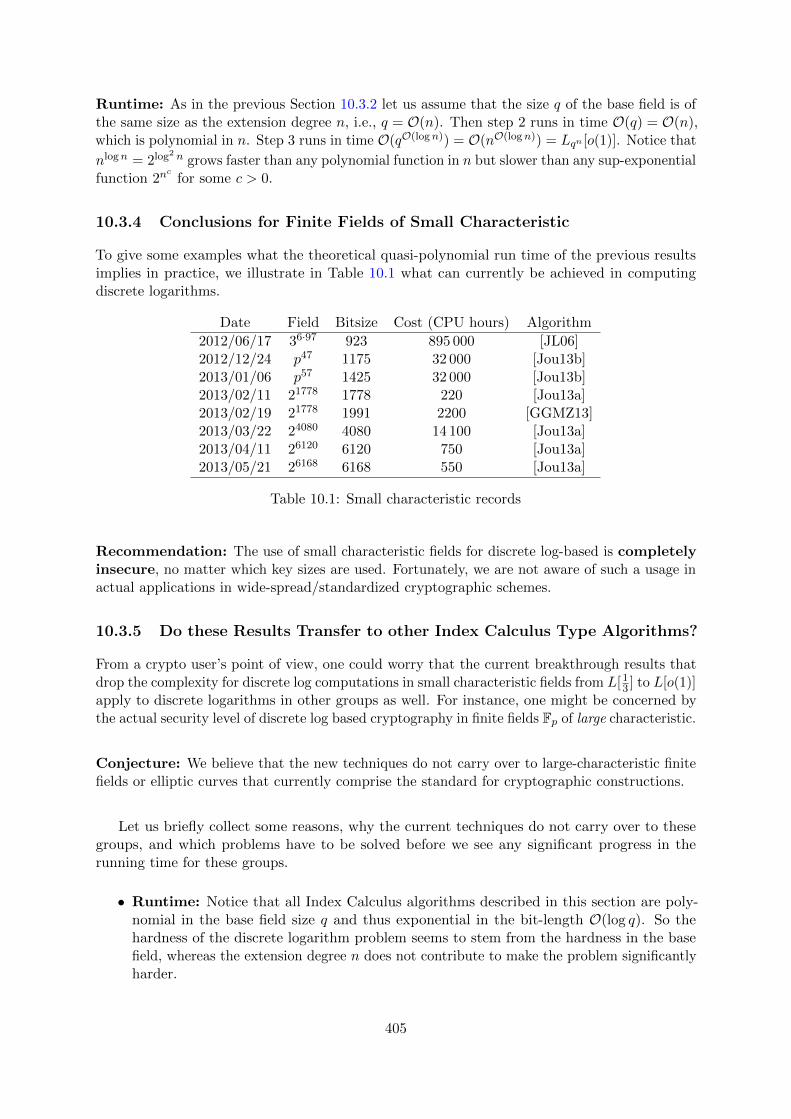
Runtime: As in the previous Section 10.3.2 let us assume that the size q of the base field is ofthe same size as the extension degree n, i.e., q = O(n). Then step 2 runs in time O(q) = O(n),which is polynomial in n. Step 3 runs in time O(qO(logn)) = O(nO(logn)) = Lqn [o(1)]. Notice that
nlogn = 2log2 n grows faster than any polynomial function in n but slower than any sup-exponential
function 2nc
for some c > 0.
10.3.4 Conclusions for Finite Fields of Small Characteristic
To give some examples what the theoretical quasi-polynomial run time of the previous resultsimplies in practice, we illustrate in Table 10.1 what can currently be achieved in computingdiscrete logarithms.
Date Field Bitsize Cost (CPU hours) Algorithm
2012/06/17 36·97 923 895 000 [JL06]2012/12/24 p47 1175 32 000 [Jou13b]2013/01/06 p57 1425 32 000 [Jou13b]2013/02/11 21778 1778 220 [Jou13a]2013/02/19 21778 1991 2200 [GGMZ13]2013/03/22 24080 4080 14 100 [Jou13a]2013/04/11 26120 6120 750 [Jou13a]2013/05/21 26168 6168 550 [Jou13a]
Table 10.1: Small characteristic records
Recommendation: The use of small characteristic fields for discrete log-based is completelyinsecure, no matter which key sizes are used. Fortunately, we are not aware of such a usage inactual applications in wide-spread/standardized cryptographic schemes.
10.3.5 Do these Results Transfer to other Index Calculus Type Algorithms?
From a crypto user’s point of view, one could worry that the current breakthrough results thatdrop the complexity for discrete log computations in small characteristic fields from L[13 ] to L[o(1)]apply to discrete logarithms in other groups as well. For instance, one might be concerned bythe actual security level of discrete log based cryptography in finite fields Fp of large characteristic.
Conjecture: We believe that the new techniques do not carry over to large-characteristic finitefields or elliptic curves that currently comprise the standard for cryptographic constructions.
Let us briefly collect some reasons, why the current techniques do not carry over to thesegroups, and which problems have to be solved before we see any significant progress in therunning time for these groups.
• Runtime: Notice that all Index Calculus algorithms described in this section are poly-nomial in the base field size q and thus exponential in the bit-length O(log q). So thehardness of the discrete logarithm problem seems to stem from the hardness in the basefield, whereas the extension degree n does not contribute to make the problem significantlyharder.
405

In particular, we note that each equation – constructed from the polynomial xq−x as donein the new small characteristic algorithms – contains at least q terms. Thus, whenever qbecomes bigger than L[1/3], even writing a single equation of this type would cost morethan the full complexity of the Number Field Sieve from Section 10.2.2.
Notice that there is a similar situation for discrete logarithms in elliptic curve groups. Whenwe use an elliptic curve over Fq in general the best known algorithm is the generic PollardRho algorithm from Chapter 10.1 with running time O(
√q). However, Gaudry’s algorithm
– that we discuss in Section 10.5.2 – requires for elliptic curves over Fqn only running time
q2−2n , which is way better than the generic bound O(q
n2 ). Like the algorithms in this
Chapter, Gaudry’s algorithm is of Index Calculus type. And similar to the algorithms inthis Chapter, the complexity of the discrete logarithm problem seems to be concentratedin the parameter q rather than the parameter n.
• Polynomials vs Numbers: Notice that the current results make heavy use of polynomialarithmetic and of subfields of Fqn . However, neither is polynomial arithmetic available forFp nor do there exist subfields for prime order groups. We would like to argue that manyproblems are efficiently solvable for polynomials, whereas they appear to be notoriouslyhard for integers. For instance, it is known that polynomials over finite fields and over therationals can be efficiently factored by the algorithms of Berlekamp and Lenstra-Lenstra-Lovasz, whereas there is no equivalent algorithm for the integers. There is also an efficientalgorithm for finding shortest vectors in polynomial rings due to von zur Gathen, whereits integer lattice counterpart is known to be NP-hard.
What makes integers intrinsically harder than polynomials is the effect of carry bits. Whenwe multiply two polynomials, we know by the convolution product exactly which coefficientscontribute to which coefficients in the product, which is not true for integer multiplicationdue to the carry bits.
• Complexity of Steps 2 & 3: Any algorithmic breakthrough for index calculus typediscrete logarithms would have to efficiently solve the discrete logarithms of a well-definedfactor base and express the desired logarithm in terms of this factor base. But currently,we do not have an efficient method for either step in the case of large prime fields Fp.
References and further reading: Coppersmith’s algorithm [Cop84] from the mid 80s wasfor a long time the reference method for computing discrete logarithms in small characteristicfields. The Joux-Lercier Function Field Sieve was introduced 2006 in [JL06].
The recent advances started at Eurocrypt 2013 with Joux’s pinpointing technique [Jou13b].At Crypto 2013, Gologlu, Granger, McGuire and Jens Zumbragel [GGMZ13] already improved theconstant c in the L[13 , c] running time. The improvement to running time L[14 ] was then presentedin the work of Joux [Jou13a]. Eventually, Barbulescu, Gaudry, Joux and Thome [BGJT13]proposed an algorithm for the decent that led to running time L[o(1)].
406

10.4 Best Known Algorithms for Factoring Integers
Management Summary: The best algorithm for factoring shows close similarity tothe best algorithm for computing discrete logarithms in prime order groups. Itseems that the new attacks do not help to improve any of the two algorithms.
The best algorithm for computing the prime factorization of integers, the so-called NumberField Sieve, is very similar to the best algorithm for computing discrete logarithm in Fp fromSection 10.2.2, and much less similar to the algorithm for Fqn from Chapter 10.3.
In a nutshell, all known, sophisticated algorithms that factor RSA moduli n = pq for primesp, q of the same size, rely on the same basic simple idea. Our goal is to construct x, y ∈ Z/nZsuch that
x2 ≡ y2 mod n and x 6≡ ±y mod n.
This immediately yields the factorization of n, since n divides the product x2−y2 = (x+y)(x−y)by the first property, but n does neither divide x+ y nor x− y by the second property. Thusone prime factor of n has to divide x+ y, whereas the other one has to divide x− y. This inturn means that gcd(x± y, n) = {p, q}.
The factorization algorithms only differ in the way in which these x, y are computed. Theintention is to compute x, y with x2 ≡ y2 mod n in an “independent” way. If this independenceis given, it is easy to show that x 6≡ ±y mod n holds with probability 1
2 , since every square inZ/nZ has 4 square roots by the Chinese Remainder Theorem – two different roots modulo pand two different roots modulo q.
10.4.1 The Number Field Sieve for Factorization (GNFS)2
Let n ∈ N be the integer that we want to factor. In the Number Field Sieve algorithm we startby constructing two polynomials f, g that share a common root m modulo N . Usually this isdone by simply defining g(X) = X −m mod n and constructing some low degree polynomialf(X) with f(m) ≡ 0 mod n (e.g. by expanding n in base m as in Section 10.2.2).
Since f and g are different, they define different rings Z[X]/f(X) and Z[X]/g(X). Butsince f and g share the same root m modulo n, both rings are isomorphic to Z/nZ; and thisisomorphism can be explicitely computed by the mapping X 7→ m. This is illustrated in thefollowing commutative diagram.
Z[X]
Q[X]/(f(X)) Q[X]/(g(X))
Z/nZ
X 7→mX 7→m
Factor base: Consists of small-norm prime elements in both number fields.
2The term number field sieve here always means the general number field sieve (GNFS). In the context offactorization there is a difference between a special and a general number field sieve – this is in the opposite tosection 10.2.2.CT2 contains an implementation of GNFS using msieve and YAFU.
407

Relation finding: We look for arguments x such that simultaneously πf := f(x) splits inQ[X]/(f(X)) and πg := g(x) splits in Q[X]/(g(X)) into the factor base. Such elementsare called relations.
Linear Algebra: By linear algebra, we search for a product of the elements πf which is a squareand whose corresponding product of the πg is also a square. If we send these elementsvia our homomorphism X 7→ m to Z/nZ, we obtain elements x2, y2 ∈ Z/nZ such thatx2 ≡ y2 mod n. If we first compute the square roots of πf and πg in their respective numberfields before applying the homomorphism, we obtain x, y ∈ Z/nZ with x2 ≡ y2 mod N , asdesired. The independence of x, y here stems from the different representations in bothnumber fields.
Runtime: The above algorithm is up to some details – e.g. the square root computation in thenumber field – identical to the algorithm of Section 10.2.2 and shares the same running time
L[13 ,(649
)1/3].
10.4.2 Relation to the Index Calculus Algorithm for Dlogs in Fp
Firstly, we know that computing discrete logarithms in composite order groups Z/nZ is at leastas hard as factoring n = pq. This in turn means that any algorithm that computes discretelogarithms in Z/nZ computes the factorization of n:
Dlogs in Z/nZ ⇒ Factoring n.
Let us briefly give the idea of this relation. We compute the order k = ord(a) for an arbitrarya ∈ Z/nZ by our dlog-algorithm, i.e. we compute the smallest positive integer k such that
ak ≡ 1 mod n. If k is even, then ak2 6≡ 1 is a square root of 1. We have a
k2 6≡ −1 with probability
at least 12 , since 1 has 4 square roots modulo n. Set x ≡ a
k2 mod n and y = 1. Then we obtain
x2 ≡ 1 ≡ y2 mod n and x 6≡ ±y mod n. By the discussion at the beginning of the Chapter thisallows us to factor n.
Secondly, we also know that both problems factoring and computing discrete logarithms inFp are together at least as hard as computing discrete logarithms in Z/nZ. In short
Factoring + Dlogs in Fp ⇒ Dlogs in Z/nZ.
This fact can be easily seen by noticing that factoring and dlogs in Fp together immediately givean efficient version of the Silver-Pohlig-Hellman algorithm from Section 10.1. We first factor thegroup order n in prime powers peii , and then compute the discrete logarithms in Fpi for eachi. Just as in the Silver-Pohlig-Hellman algorithm we lift the solution modulo peii and combinethese lifted solutions via Chinese Remaindering.
We would like to stress that these two known relations do not tell much about whether thereis a reduction
Factoring ⇒ Dlog in Fp or Dlog in Fp ⇒ Factoring.
Both directions are a long-standing open problem in cryptography. Notice however that the bestalgorithms for factoring and dlog in Fp from Sections 10.2.2 and 10.4.1 are remarkably similar.Also historically always algorithmic progress for one problem immediately implied progress forthe other problem as well. Although we have no formal proof, it seems to be fair to say thatboth problems seem to be closely linked from an algorithmic perspective.
408

10.4.3 Integer Factorization in Practice
Given the current state of the art of academic integer factorization research, even moderatelysized – but properly chosen – RSA moduli offer a reasonable amount of protection against opencommunity cryptanalytic efforts. The largest RSA challenge number factored by a public efforthas just 768 bits [KAF+10] and required the equivalent of about 2000 years of computing ona single 2 GHz core. Attacking a 1024-bit RSA modulus is about a thousand times harder.Such an effort must be expected to be out of reach for academic efforts for several more years.Doubling the size to 2048-bit moduli increases the computational effort by another factor of 109.Without substantial new mathematical or algorithmic insights 2048-bit RSA must be consideredto be out of reach for at least two more decades.
10.4.4 Relation of Key Size vs. Security for Dlog in Fp and Factoring
The running time of the best algorithm for a problem defines the security level of a cryptosystem.E.g. for 80-bit security, we want that the best algorithm requires at least 280 steps.
As we already noted, the best running time for discrete logs in Fp and for factoring is
L[13 ,(649
)1/3]. The most accurate way to use this formula is to actually measure the running
time for a large real world factorization/dlog computation, and then extrapolate to large values.Assume that we know that it took time T to factor a number n1, then we extrapolate the runningtime for some n2 > n1 by the formula
T ·Ln1 [13 ,
(649
)1/3]
Ln2 [13 ,(649
)1/3].
So, we use the L-formula to estimate the relative factor that we have to spend in addition.Notice that this (slightly) overestimates the security, since the L-formula is asymptotic and thusbecomes more accurate in the numerator than in the denominator – the denominator shouldinclude a larger error term. So in practice, one obtains (only slightly) less security than predictedby this formula.
We computed the formula for several choices of the bit-size of an RSA number n, respectivelya dlog prime p, in Table 10.2. Recall from Section 10.4.1 that the running time of the NumberField Sieve algorithm for factoring is indeed a function of n and not of the prime factors of n.
We start with RSA-768 that has been successfully factored in 2009 [KAF+10]. In order tocount the number of instructions for factoring RSA-768, one has to define what an instructionunit is. It is good practice in cryptography to define as a unit measure the time to evaluate DESin order to obtain comparability of security levels between secret and public key primitives. Thenby definition of this unit measure, DES offers 56-bit security against brute-force key attacks.
In terms of this unit measure, the factorization of RSA-768 required T = 267 instructions.From this starting point, we extrapolated the security level for larger bit-sizes in Table 10.2.
We successively increase the bit-size by 128 up to 2048 bits. We see that in the beginning,this leads to roughly an increase of security of 5 bits per 128-bit step, whereas in the end weonly have an increase of roughly 3 bits per 128-bit step.
By Moore’s law the speed of computers doubles every 1.5 years. Hence after 5 · 1.5 = 7.5years we have an increase of 25, which means that currently we should roughly increase ourbit-size by 128 bits every 7.5 years; and when we come closer to 2000 bits our increase of 128-bitsteps should be in intervals of no later than 4.5 years. For more conservative choices that also
409

bit-size security
768 67.0896 72.41024 77.31152 81.81280 86.11408 90.11536 93.91664 97.51792 100.91920 104.22048 107.4
Table 10.2: Bitsize of n, p versus security level
anticipate some algorithmic progress rather than just an increase in computers’ speed see therecommendations in Chapter 10.7.
References and further reading: An introduction to several factorization algorithms includ-ing the Quadratic Sieve – the predecessor of the Number Field Sieve – can be found in May’slecture notes on number theory [May13]. We recommend Blomer’s lecture notes on algorithmicnumber theory [Blo99] as an introduction to the Number Field Sieve.
The development of the Number Field Sieve is described in the textbook of Lenstra andLenstra [LL93] that includes all original papers. The relation of discrete logarithms and factoringhas been discussed by Bach [Bac84]. Details of the current factorization record for RSA-768 canbe found in [KAF+10].
410

10.5 Best Known Algorithms for Elliptic Curves E
Management Summary: Elliptic curves are the second standard group for the dis-crete logarithm problem. The new attacks do not affect these groups, their securityremains unchanged.
We would like to discuss elliptic curves E[pn] over finite extension fields Fpn and elliptic curvesE[p] over prime fields Fp. The later are usually used for cryptographic purposes. The reason todiscuss the former too is to illustrate – similar to the previous chapters – the vulnerabilities ofextension fields Fpn as opposed to prime field Fp. However, we would like to point out that weassume in the following – in contrast to the previous chapter – that n is fixed. This is because asopposed to the algorithm of Joux et al, the algorithms for E[pn] have complexities which dependexponentially on n.
We present two different approaches for elliptic curves over extension fields: cover (or Weildescent) attacks introduced by Gaudry, Hess and Smart (GHS), and decomposition attacksproposed by Semaev and Gaudry. In some cases, it is possible to combine the two approachesinto an even more efficient algorithm as shown by Joux and Vitse [JV11].
10.5.1 The GHS Approach for Elliptic Curves E[pn]
This approach introduced by Gaudry, Hess and Smart aims at transporting the discrete logarithmproblem from an elliptic curve E defined over an extension field Fpn to an higher genus curvedefined over a smaller field, for example Fp. This can be done by finding a curve H over Fptogether with a surjective morphism from H to E. In this context, we say that the curve H is acover of E. Once such a curve H is obtained, it is possible using the so called coNorm techniqueto pulI back a discrete logarithm problem on E to a discrete logarithm problem on the Jacobianof H. If the genus g of the target curve is not too large, this can lead to an efficient discretelogarithm algorithm. This uses the fact that there exists an index calculus algorithm on highgenus curve of genus g over Fp with complexity max(g! p, p2). This was introduced by Enge,Gaudry and Thome [EGT11].
Ideally, one would like the genus g to be equal to n. However, this is not possible in general.Classifying the possible covers for elliptic curve seems to be a difficult task.
10.5.2 Gaudry-Semaev Algorithm for Elliptic Curves E[pn]
Let Q = αP be a discrete logarithm on an elliptic curve E[pn]. So the goal is to find the integerα ∈ N such that k times the point P ∈ E[pn] added to itself is equal to the point Q ∈ E[pn].
Gaudry’s discrete logarithm algorithm is of index calculus type. We briefly outline the basicsteps.
Factor base: Consists of all points (x, y) on the elliptic curve E[pn] such that x ∈ Fp. That isx lies in the ground field Fp rather than in the extension.
Relation finding: Given a random point R = aP , with a ∈ N, we try to write R as a sum ofexactly n points from the factor base, where n is the extension degree. This is achieved byusing the n-th Semaev polynomial fn+1. This polynomial is a symmetric polynomial ofdegree 2n−2 in n+1 unknowns x1, . . . , xn+1 which encodes the fact that there exists pointswith respective abscissae x1, . . . , xn+1 which sum to zero. Of course, the coefficients of f
411
depend on the curve E. Replacing xn+1 by the abscissa of R, we can find a decompositionof R as a sum of points from the factor base by searching for a solution (x1, · · · , xn) inthe basefield Fp. In order to do this, one first rewrites f as a multivariate system of nequations by decomposing the constants that appear in the polynomial over some basis ofFpn over Fp. This system of n equations in n unknowns can be solved using a Grobnerbasis computation.
Individual Discrete Log Computation: To compute the discrete logarithm of Q, it sufficesto find one additional relation that express a random multiple of Q, namely R = aQ interms of the points in the factor base. This is done in the exact same way as the generationof relations in the previous step.
Runtime: The factor base can be computed in time O(p). Every R can be written as a sumof n factor base elements, i.e. yields a relation, with probability exponentially small in n (butindependent of p). If it yields a solution the running time of a Grobner basis computation isalso exponential in n (but polynomial in log p). In total, we need roughly p relations which canbe computed in time linearly in p and exponentially in n. Since we assumed n to be fixed, we donot care about the bad behavior in n. The linear algebra step on a (p× p)-matrix can then beperformed in O(p2), since the matrix is sparse – every row contains exactly n non-zero entries.
With additional tricks one achieves a running time of O(p2−2n ) for Gaudry’s algorithm.
This should be compared to the generic bound of O(pn2 ) that we achieve when using Pollard’s
Rho algorithm from Chapter 10.1. Similar to Chapter 10.3, almost the whole complexity of theproblem seems to be concentrated in the size of the base field p, and not in the extension degreen. Notice that as in Chapter 10.3, Gaudry’s algorithm is exponential in log p.
10.5.3 Best Known Algorithms for Elliptic Curves E[p] over Prime Fields
Generic discrete log solving: In general, the best algorithm that we know for arbitraryelliptic curves E[p] is Pollard’s Rho method with a running time of O(
√p). For the moment, it
seems that nobody knows how to exploit the structure of an elliptic curve group or its elementsin order to improve over the generic bound.
We would also like to point out that random elliptic curves, i.e. where the elliptic curveparameters a, b in the defining Weierstrass equation y2 ≡ x3 + ax + b mod p are chosen in auniformly random manner, are among the hard instances. To further harden elliptic curves, onechooses for standardization only those curves that have (almost) prime order. This means thatthe co-factor of the largest prime in the group order is usually 1, which abandons the use ofSilver-Pohlig-Hellman’s algorithm.
Embedding E[p] into Fpk : It is known that in general elliptic curves E[p] can be embeddedinto a finite field Fpk , where k is the so-called embedding degree. In Fpk we could use the NumberField Sieve for discrete logarithm computations. Hence such an embedding would be attractiveif Lpk [
13 ] is smaller than
√p, which is the case only if the embedding degree k happens to be
very small. However, for almost all elliptic curves the embedding degree is known to be huge,namely comparable to p itself.
Some constructions in cryptography, e.g. those that make use of bilinear pairings, exploitthe advantages of a small embedding degree. Thus, in these schemes elliptic curves are explicitlychosen with a small embedding degree, e.g. k = 6, which balances out the hardness of thediscrete logarithm problem on E[p] and in Fkp.The xedni calculus algorithm: In 2000, Silverman published his xedni calculus algorithm
412
(read xedni backwards) that uses the group structure of E[p] for discrete logarithm computations,and thus is the only known non-generic algorithm that works directly on E[p]. However, it wassoon after his publication discovered that the so-called lifting process in Silverman’s algorithmhas a negligible probability of succeeding in computing a discrete logarithm.
10.5.4 Relation of Key Size vs. Security for Elliptic Curves E[p]
Similar to the discussion in Section 10.4.4 about key sizes for dlog in Fp and for factoring, wewant to evaluate how key sizes have to be adapted for elliptic curves E[p] in order to guardagainst an increase in computer speed. For elliptic curves, such an analysis is comparably simple.The best algorithm that we know for the dlog in E[p] is Pollard’s Rho method with running time
Lp[1,1
2] =√p = 2
log p2 .
This means that for achieving a security level of k bits, we have to choose a prime p with 2kbits. In other words, increasing the bit-size of our group by 2 bits leads to increase of 1 bitin security. By Moore’s law we loose 1 bit of security every 1.5 years just from an increase ofcomputer’s speed. In order to guard against this loss over 10 years, it thus suffices to increasethe group-size by just 7 · 2 = 14 bits. Notice that as opposed to the case of dlog in Fp andfactoring in Section 10.4.4 this increase is linear and independent of the starting point. Thatmeans to guard against technological speedups over 20 years, an increase of 28 bits is sufficient.
Of course, this analysis only holds if we do not have to face any major breakthrough incomputer technology or algorithms. For a more conservative choice see the advice in Chapter 10.7.
10.5.5 How to Securely Choose Elliptic Curve Parameters
A comprehensive description on how to choose elliptic curve domain parameters over finite fieldscan be found in RFC 5639 “ECC Brainpool Standard Curves and Curve Generation” by ManfredLochter and Johannes Merkle [LM10, LM05]. This RFC defines a publicly verifiable way ofchoosing pseudo-random parameters for elliptic curve parameters, and thus it excludes the mainsource for embedding a trapdoor in the definition of a group. The authors discuss all knownproperties of a curve E[p] that might potentially weaken its security:
• A small embedding degree for the embedding into a finite field. This would allowfor the use of more efficient finite field algorithms. Especially, the requirement excludessupersingular curves of order p+ 1.
• Trace one curves which have order |E[p]| = p. These curves are known to be weak by thediscrete logarithm algorithms of Satoh-Araki [SA98], Semaev [Sem98] and Smart [Sma99].
• Large class number. This excludes that E[p] can be efficiently lifted to a curve definedover some algebraic number field. This requirement is quite conservative, since even forsmall class numbers there is currently no efficient attack known.
Moreover the authors insist on the following useful properties.
• Prime order. This simply rules out subgroup attacks.
• Verifiable pseudo random number generation. The seeds for a pseudo randomnumber generator are chosen in a systematic way by Lochter and Merkle, who use in
413
their construction the first 7 substrings of lenght 160 bit of the fundamental constantπ = 3.141 . . ..
In addition, Lochter and Merkle specify a variety of curves for p’s of bit-lengths in the range 160to 512. For TLS/SSL there is also a new set of proposed Brainpool curves available [LM13].
The work of Bos, Costello, Longa and Naehrig [BCLN14] gives a valuable introduction forpractitioners on how to choose elliptic curve parameters that are secure and also allow forefficient implementation in various coordinate settings (Weierstrass, Edwards, Montgomery).Additionally, Bos et al focus on side-channel resistance against timing attacks by proposingconstant-time scalar multiplications.
We highly recommend the SafeCurve project by Daniel Bernstein and Tanja Lange [BL14]that provides an excellent overview for several selection methods, their benefits and drawbacks.The goal of Bernstein and Lange is to provide security of Elliptic Curve Cryptography – ratherthan just strength of elliptic curves against discrete logarithm attacks. Therefore, they take intoaccount various types of side-channels that may leak secrets in an implementation.
References and further reading: For an introduction to the mathematics of elliptic curvesand their cryptographic applications we refer to the textbooks of Washington [Was08], Gal-braith [Gal12], and Silverman [Sil99].
This section described the results of the original works of Gaudry, Hess, Smart [GHS02],Gaudry [Gau09], Semaev [Sem04], and the xedni algorithm of Silverman [Sil99].
414

10.6 Possibility of Embedded Backdoors in Cryptographic Keys
Management Summary: All cryptography seems to offer the possibility of embed-ding backdoors. Dlog schemes offer some advantage over factoring-based schemesin the sense that carefully chosen system-wide parameters protect all users.
The possibility of embedding trapdoors in cryptographic schemes to bypass cryptography andthus to decrypt/sign/authenticate without the use of a secret key is a long recognized problemthat has been intensively discussed in the cryptographic community – e.g. at the panel discussionat Eurocrypt 1990. However, the wide-spread use of NSA’s backdoors as described by EdwardSnowden has recently renewed the interest in this topic.
It appears that by construction some schemes are way more vulnerable than others. E.g. fordiscrete-log based schemes the definition of the group parameters is a system-wide parameterthat is used by any user in the scheme. Thus, a party that is able to manipulate the definitionof a group in such a way that enables this party to compute discrete logarithms in this groupefficiently, can decrypt all communication. On the other hand, a carefully specified secure groupalso offers security for all users.
Currently, there is some speculation whether the NSA influenced NIST, the U.S. standard-ization agency, to standardize certain elliptic curves. But the definition of a group is not theonly way to embed backdoors. All cryptographic schemes rely inherently on a good source of(pseudo-)random bits. It is well known that so-called semantic security of encryption schemescannot be achieved without randomness, and every cryptographic secret key is assumed tobe randomly chosen. Thus a weak pseudo-random generator opens the door for bypassingcryptography. Such a weak pseudo-random generator was standardized by NIST as SpecialPublication 800-90, although there have been warnings by the cryptographic community.
For factoring-based schemes the situation is slightly different than for discrete log-basedschemes. As opposed to discrete log schemes, there are no system-wide parameters that define agroup. Nevertheless, there are known ways to embed e.g. information about the factorization ofthe RSA modulus N in the RSA public exponent e. Moreover, recent attacks on RSA publickey infrastructures [LHA+12, HDWH12] show that it appears to be a difficult problem togenerate RSA public keys with different primes in the public, mainly due to bad initializationsof pseudo-random generators. This of course does only affect badly chosen keys of individuals asopposed to all users of cryptographic scheme.
Recommendation: Dlog-based schemes seem to be easier to control from a crypto designersperspective, since here all users have to take the same system-wide parameters.
We do not discuss the possibility of malware here – which may render obsolete any crypto-graphic protection method – or how to protect against it. But we would like to stress the follow(somewhat trivial) warning that addresses a crucial point in practice.
Warning: Cryptography can only protect data if it is properly implemented and does not leakits (immanent) secret. So in addition to the mathematical hardness of the underlying problems,we also have to trust in the implementor of a cryptographic scheme. This trust does not onlyinclude that the cryptographic scheme is implemented in the way it was originally designed– without embedding of any backdoors –, but also that the implementor does not reveal the
415

generated secret keys to a third party.
It seems that in the NSA affair, some companies were forced to reveal secret keys. Thus,one has to keep in mind that one has to buy cryptographic schemes from a completely reliablecompany that has not been compromised.
References and further reading: For a nice discussion of how to embed undetectablebackdoors in various cryptographic schemes, see the original works of Young and Yung [YY96,YY97]. See [LHA+12] for a current attack on a significant portion of RSA keys in practice dueto bad pseudo random number generation.
416

10.7 Advice for Cryptographic Infrastructure
Management Summary: Despite of recent discrete logarithm attacks, discretelogarithm-based schemes over prime order groups and elliptic curve groups remainsecure. The same holds for factoring-based schemes. All discrete logarithm-basedgroups with small characteristic are completely insecure. Our suggestion is tochoose elliptic curve groups.
10.7.1 Suggestions for Choice of Scheme
As we saw in the previous Chapters, discrete log-based schemes in Fp and over E[p] remain secure,as well as factoring-based schemes. In the following, we suggest key sizes for these schemes thatprovide a sufficient security level for the next two decades under the assumption that nomajor algorithmic breakthrough occurs.
System Key size in bits
Dlog in Fp 2000 until 2019, then 3000Factoring 2000 until 2019, then 3000
Dlog in E[p] 224 until 2015, then 250
Table 10.3: Security level 100 bit, source: BSI [BSI12], ANSSI [Age13]
Our preference is to use elliptic curve groups E[p] since they offer the following advantages:
• Algorithms for discrete logarithms in Fp and factoring are closely linked. So any progressin one of these two might imply some progress for the other. But such a progress is unlikelyto affect the security of elliptic curve groups.
• The best algorithms for E[p] are those of generic type from Chapter 10.1, which are inferiorto the best algorithms for prime order discrete logarithm and factoring with L[13 ] runningtime. This in turn means that the key growth that compensates technological progress offaster computers is much smaller for E[p] – roughly 2 bits every 1.5 years according toMoore’s law.
• Getting algorithmic progress by using the group structure of E[p] seems to be harder thanfor Fp, since as opposed to Fp we do not even have an initial starting group-structure IndexCalculus algorithm that we could improve.
• If an elliptic curve E[p] is properly chosen, i.e. the group is computationally hard andbackdoor-free, then all users profit from the hardness of the discrete logarithm problem.Notice that this choice is crucial: If the group is not secure, then also all users suffer fromits insecurity.
Warning: One should keep in mind that the suggestions above only hold in a world withoutlarge quantum computers. It seems crucial to keep track of current progress in this area, and tohave some alternative quantum-resistant cryptosystems ready to enroll within the next 15 years.
References and further reading: For a good and conservative choice of key sizes we highlyrecommend to follow the suggestions of the Bundesamt fur Sicherheit in der Informationstechnik(BSI) [BSI12] and the Agence nationale de la securite des systemes d’information [Age13]. Both
417

sources also provide various valuable recommendations how to correctly implement and combinedifferent cryptographic primitives.
Remark from the editor in June 2016: Since April 2014, quite a lot of things have changed(there have been new records in dlog finite fields and some marginal improvements of the L(1/3)algorithms in some contexts). However, this does not affect the overall conclusion that (only)small characteristic finite fields are no longer secure.
418
Bibliography (Chap DLogFact)
[Adl79] Adleman, Leonard M.: A Subexponential Algorithm for the Discrete LogarithmProblem with Applications to Cryptography (Abstract). In FOCS, pages 55–60, 1979.
[Age13] Agence nationale de la securite des systemes d’information: Referentiel general desecurite Version 2.02, 2013.http://www.ssi.gouv.fr/administration/reglementation/.
[Bac84] Bach, Eric: Discrete Logarithms and Factoring. Technical Report UCB/CSD-84-186,EECS Department, University of California, Berkeley, June 1984.http://www.eecs.berkeley.edu/Pubs/TechRpts/1984/5973.html,http://www.eecs.berkeley.edu/Pubs/TechRpts/1984/CSD-84-186.pdf.
[BCLN14] Bos, Joppe W., Craig Costello, Patrick Longa, and Michael Naehrig: SelectingElliptic Curves for Cryptography: An Efficiency and Security Analysis, 2014.Microsoft Research.https://www.microsoft.com/en-us/research/wp-content/uploads/2016/02/
selecting.pdf.
[BGJT13] Barbulescu, Razvan, Pierrick Gaudry, Antoine Joux, and Emmanuel Thome: A quasi-polynomial algorithm for discrete logarithm in finite fields of small characteristic.CoRR, abs/1306.4244, 2013.
[BL14] Bernstein, Daniel and Tanja Lange: SafeCurves: choosing safe curves for elliptic-curve cryptography. http://safecurves.cr.yp.to/, 2014.
[Blo99] Blomer, J.: Vorlesungsskript Algorithmische Zahlentheorie, 1999. Ruhr-UniversityBochum.http://www.math.uni-frankfurt.de/~dmst/teaching/lecture_notes/bloem
er.algorithmische_zahlentheorie.ps.gz.
[BSI12] BSI (Bundesamt fur Sicherheit in der Informationstechnik): BSI TR-02102Kryptographische Verfahren: Empfehlungen und Schlussellangen, 2012.https://www.bsi.bund.de/DE/Publikationen/TechnischeRichtlinien/tr
02102/index_htm.
[Cop84] Coppersmith, Don: Evaluating Logarithms in GF (2n). In STOC, pages 201–207,1984.
[COS86] Coppersmith, Don, Andrew M. Odlyzko, and Richard Schroeppel: Discrete Loga-rithms in GF(p). Algorithmica, 1(1):1–15, 1986.
[EGT11] Enge, Andreas, Pierrick Gaudry, and Emmanuel Thome: An L(1/3) Discrete Loga-rithm Algorithm for Low Degree Curves. J. Cryptology, 24(1):24–41, 2011.
419

[FJM14] Fouque, Pierre Alain, Antoine Joux, and Chrysanthi Mavromati: Multi-user colli-sions: Applications to Discrete Logarithm, Even-Mansour and Prince. CryptologyePrint Archive, 2014. https://eprint.iacr.org/2013/761.
[Gal12] Galbraith, Steven D.: Mathematics of Public Key Cryptography. Cambridge Univer-sity Press, 2012, ISBN 9781107013926.
[Gau09] Gaudry, Pierrick: Index calculus for abelian varieties of small dimension and theelliptic curve discrete logarithm problem. J. Symb. Comput., 44(12):1690–1702, 2009.
[GGMZ13] Gologlu, Faruk, Robert Granger, Gary McGuire, and Jens Zumbragel: On theFunction Field Sieve and the Impact of Higher Splitting Probabilities – Applicationto Discrete Logarithms. In CRYPTO (2), pages 109–128, 2013.
[GHS02] Gaudry, Pierrick, Florian Hess, and Nigel P. Smart: Constructive and DestructiveFacets of Weil Descent on Elliptic Curves. J. Cryptology, 15(1):19–46, 2002.
[HDWH12] Heninger, Nadia, Zakir Durumeric, Eric Wustrow, and J. Alex Halderman: MiningYour Ps and Qs: Detection of Widespread Weak Keys in Network Devices. InProceedings of the 21st USENIX Security Symposium, August 2012.https://factorable.net/paper.html.
[Hom07] Homeister, Matthias: Quantum Computer Science: An Introduction.Vieweg+Teubner Verlag, 2007, ISBN 9780521876582.
[JL06] Joux, Antoine and Reynald Lercier: The Function Field Sieve in the Medium PrimeCase. In EUROCRYPT, pages 254–270, 2006.
[Jou09] Joux, Antoine: Algorithmic Cryptanalysis. CRC Cryptography and Network SecuritySeries. Chapman & Hall, 2009, ISBN 1420070029.
[Jou13a] Joux, Antoine: A new index calculus algorithm with complexity L(1/4+o(1)) in verysmall characteristic. IACR Cryptology ePrint Archive, 2013:95, 2013.
[Jou13b] Joux, Antoine: Faster Index Calculus for the Medium Prime Case Application to1175-bit and 1425-bit Finite Fields. In EUROCRYPT, pages 177–193, 2013.
[JV11] Joux, Antoine and Vanessa Vitse: Cover and Decomposition Index Calculus onElliptic Curves made practical. Application to a seemingly secure curve over Fp6 .IACR Cryptology ePrint Archive, 2011:20, 2011.
[KAF+10] Kleinjung, Thorsten, Kazumaro Aoki, Jens Franke, Arjen K. Lenstra, EmmanuelThome, Joppe W. Bos, Pierrick Gaudry, Alexander Kruppa, Peter L. Montgomery,Dag Arne Osvik, Herman J. J. te Riele, Andrey Timofeev, and Paul Zimmermann:Factorization of a 768-Bit RSA Modulus. In CRYPTO, pages 333–350, 2010.
[LHA+12] Lenstra, Arjen K., James P. Hughes, Maxime Augier, Joppe W. Bos, ThorstenKleinjung, and Christophe Wachter: Public Keys. In CRYPTO, pages 626–642, 2012.
[LL93] Lenstra, A. K. and H. W. Jr. Lenstra: The Development of the Number Field Sieve.Lecture Notes in Mathematics. Springer Verlag, 1993, ISBN 0387570136.
[LM05] Lochter, Manfred and Johannes Merkle: ECC Brainpool Standard Curves and CurveGeneration v. 1.0, 2005.www.ecc-brainpool.org/download/Domain-parameters.pdf.
420

[LM10] Lochter, Manfred and Johannes Merkle: Elliptic Curve Cryptography (ECC) Brain-pool Standard Curves and Curve Generation, 2010. RFC 5639.http://www.rfc-base.org/txt/rfc-5639.txt.
[LM13] Lochter, Manfred and Johannes Merkle: Elliptic Curve Cryptography (ECC) Brain-pool Curves for Transport Layer Security (TLS), 2013. RFC 7027.http://tools.ietf.org/search/rfc7027.
[May08] May, Alexander: Vorlesungsskript Kryptanalyse 1, 2008. Ruhr-University Bochum.http://www.cits.ruhr-uni-bochum.de/imperia/md/content/may/pkk08/skri
pt.pdf.
[May12] May, Alexander: Vorlesungsskript Kryptanalyse 2, 2012. Ruhr-University Bochum.http://www.cits.ruhr-uni-bochum.de/imperia/md/content/may/12/ws1213/
kryptanal12/kryptanalyse_2013.pdf.
[May13] May, Alexander: Vorlesungsskript Zahlentheorie, 2013. Ruhr-University Bochum.http://www.cits.ruhr-uni-bochum.de/imperia/md/content/may/13/ss13/za
hlenss13/zahlentheorie.pdf.
[Mer08] Mermin, David N.: Quantum Computing verstehen. Cambridge University Press,2008, ISBN 3834804363.
[MSP11] Muller-Stach and Piontkowski: Elementare und Algebraische Zahlentheorie. ViewegStudium, 2011, ISBN 3834882631.
[MvOV01] Menezes, Alfred J., Paul C. van Oorschot, and Scott A. Vanstone: Handbook ofApplied Cryptography. Series on Discrete Mathematics and Its Application. CRCPress, 5th edition, 2001, ISBN 0-8493-8523-7. (Errata last update Jan 22, 2014).http://cacr.uwaterloo.ca/hac/,http://www.cacr.math.uwaterloo.ca/hac/.
[Pol75] Pollard, John M.: A Monte Carlo method for factorization. BIT Numerical Mathe-matics 15, 3:331–334, 1975.
[Pol00] Pollard, John M.: Kangaroos, Monopoly and Discrete Logarithms. J. Cryptology,13(4):437–447, 2000.
[Pom84] Pomerance, Carl: The Quadratic Sieve Factoring Algorithm. In Blakley, G.R. andD. Chaum (editors): Proceedings of Crypto ’84, LNCS 196, pages 169–182. Springer,1984.
[Pom96] Pomerance, Carl: A tale of two sieves. Notices Amer. Math. Soc, 43:1473–1485,1996.
[PRSS13] Ptacek, Thomas, Tom Ritter, Javed Samuel, and Alex Stamos: The Factoring Dead– Preparing for the Cryptopocalypse. Black Hat Conference, 2013.
[SA98] Satoh, T. and K. Araki: Fermat Quotients and the Polynomial Time Discrete LogAlgorithm for Anomalous Elliptic Curves. Commentarii Mathematici UniversitatisSancti Pauli 47, 1998.
[Sem98] Semaev, I.: Evaluation of Discrete Logarithms on Some Elliptic Curves. Mathematicsof Computation 67, 1998.
421

[Sem04] Semaev, Igor: Summation polynomials and the discrete logarithm problem on ellipticcurves. IACR Cryptology ePrint Archive, 2004:31, 2004.
[Sho94] Shor, Peter W.: Algorithms for Quantum Computation: Discrete Logarithms andFactoring. In FOCS, pages 124–134, 1994.
[Sho97] Shoup, Victor: Lower Bounds for Discrete Logarithms and Related Problems. InEUROCRYPT, pages 256–266, 1997.
[Sil99] Silverman, Joseph H.: The Xedni Calculus And The Elliptic Curve Discrete LogarithmProblem. Designs, Codes and Cryptography, 20:5–40, 1999.
[Sma99] Smart, N.: The Discrete Logarithm Problem on Elliptic Curves of Trace One. Journalof Cryptology 12, 1999.
[Was08] Washington, Lawrence C.: Elliptic Curves: Number Theory and Cryptography.Discrete Mathematics and its Applications. Chapman and Hall/CRC, 2008,ISBN 9781420071467.
[YY96] Young, Adam L. and Moti Yung: The Dark Side of Black-Box Cryptography, or:Should We Trust Capstone? In CRYPTO, pages 89–103, 1996.
[YY97] Young, Adam L. and Moti Yung: Kleptography: Using Cryptography against Cryp-tography. In EUROCRYPT, pages 62–74, 1997.
All links have been confirmed at July 15, 2016.
422

Chapter 11
Crypto 2020 — Perspectives forLong-Term Cryptographic Security
(Johannes Buchmann, Erik Dahmen, Alexander May, and Ulrich Vollmer, TU Darmstadt,May 2007)
Cryptography is a basic building block of all IT security solutions. Yet, for how long are thecryptographic tools we use today going to remain secure? Is this time long enough to ensure theconfidentiality of medical data, to name just one example? Even in the short-term, the potentialfor havoc is great if certain keys are broken. Just think of the digital signatures that protect theauthenticity of automatic updates for the Windows operating system.
11.1 Widely used schemes
In 1978, Rivest, Shamir and Adleman suggested the RSA public key encryption and signatureschemes [RSA78]. RSA is still the most widely used public key scheme. The security of RSAdepends on the difficulty of factoring so-called RSA moduli which are products of two largeprime numbers. In their 1978 paper, the inventors of RSA suggested the use of RSA moduliwith 200 decimal digits for long-term security. Later, the company RSA Security publisheda list of RSA moduli of increasing size, the RSA Challenge numbers. RSA Security offeredprizes totaling $ 635,000 for the factorization of these numbers, cf. http://www.emc.com/emc-plus/rsa-labs/historical/the-rsa-challenge-numbers.htm.
In 2005, that is 27 years after the invention of RSA, Bahr, Boehm, Franke, and Kleinjungfrom Bochum University managed to factor a 200 digit RSA challenge number (www.mat.uniroma2.it/~eal/rsa640.txt). A key with size originally thought to be secure for a very long timewas broken with a computation that took them just five months. This illustrates the tremendousprogress factoring technology has made within the last 30 years. This progress is based onbreak-through mathematical ideas — e.g. the number field sieve proposed by John Pollard — aswell as significant developments in computer hardware and software implementation technology.1
In 2000, Lenstra and Verheul developed an extrapolation formula that is supposed to help usforecast the security one can achieve with RSA and other important cryptographic schemes inthe long term (www.keylength.com). The formula suggests the use of 850 digit RSA moduli if
1Please compare chapter 4.11 Considerations regarding the security of the RSA algorithm, and especially chapters4.11.4 and 4.11.5. For current cryptanalytical results against RSA and Dlog see chapter 10.
423

one wishes to protect data for the next 30 years. This corresponds to a 3072 bit RSA key.
Yet, even a well thought out extrapolation formula is no security guarantee! At any time, abrilliant mathematical idea can allow us to factor large numbers easily, and destroy the securityof RSA. In 1996, Peter Shor showed that a quantum computer — a new type of computerthat leverages the laws of quantum mechanics to speed up certain types of computations —can in principle be used for the fast factorization of large numbers [Sho97]. Despite intensiveresearch in the area, it is still too early to judge whether we are ever going to be able to buildquantum computers of sufficient capacity to apply Shor’s algorithm to numbers of relevant size.2
Recent announcements of significant progress in this area made by the start-up company D-Wave(www.dwavesys.com) have been greeted with a lot of scepticism, even ridicule.
The development of attacks on another frequently used scheme called DSA (Digital SignatureAlgorithm) and the Elliptic Curve Cryptography (ECC) class of schemes moves in analogy tothose on RSA. The security of these schemes depends on the difficulty of computing discretelogarithms. Even today, there is significant algorithmic progress. Quantum computers wouldrender these schemes insecure.
What’s the state of affairs with the so-called secret-key encryption schemes? In 1977, DESwas introduced as the Data Encryption Standard [DES77]. Twenty-one years later, the ElectronicFrontier Foundation (EFF) built the special purpose machine Deep Crack which needed just 56hours to break a DES key. The problem with DES was that it used keys which were too short.It seems that the inventors of DES did not foresee the speed of hardware development. TheAdvanced Encryption Standard AES [AES02], successor to DES, is deemed secure at the momenteven though there are interesting, if still inefficient, methods to attack AES with algebraicmethods.
11.2 Preparation for tomorrow
Is the security of today’s cryptography measuring up to its increasing importance? The experienceshows: Carefully designed and implemented cryptographic schemes have a life time of five totwenty years. Whoever uses RSA, ECC or AES for short-term protection of data may feel safe.Moreover, it is also possible to achieve long-term authenticity, integrity and non-reputability ofdata, e.g., using the multiple signature scheme suggested by Sonke Maseberg [Mas02].
However, current schemes cannot guarantee long-term confidentiality. And what is to be donein twenty years from now? What should we do if, quasi over-night, unexpected mathematicalprogress renders an important cryptographic scheme insecure? Three things are necessary toprepare us for this event:
• a pool of secure alternative cryptographic schemes,
2Required qbits for attacks on RSA, DSA and ECDSA using key with a bit length n:
RSA 2n + 3DSA 2n + 3
ECDSA 2n ˜2n + 8 log nECDSA p ˜4n
Please compare chapter 5.3 in “SicAri – Eine Sicherheitsplattform und deren Werkzeuge fur die ubiquitareInternetnutzung, KB2.1 – Abschlussbericht, Ubersicht uber Angriffe auf relevante kryptographische Verfahren”,version 1.0, Mai 17, 2005, Prof. Dr. Johannes Buchmann et al., TUD-KryptC and cv cryptovision GmbH(http://www.cdc.informatik.tu-darmstadt.de/~schepers/kb_21_angriffe.pdf) and the dissertation of AxelSchmidt at the same faculty.
424

• infrastructures that enable us to exchange one cryptographic scheme for another, easilyand quickly, and
• methods that ensure long-term confidentiality.
For many years, the cryptography group at the Technische Universitat Darmstadt andits spin-off, the company FlexSecure (www.flexsecure.de), have worked to provide thesetools. The trust center software FlexiTrust which is employed by the German National RootCertification Authority and the German Country Signing Authority offers an infrastructure withinwhich cryptographic schemes can be easily exchanged. The open source library FlexiProviderimplements a multitude of cryptographic schemes. Lately, we have intensified our research into“Post Quantum Cryptography” (PQC) seeking cryptographic schemes which remain secure evenin the event that powerful quantum computers are built.
The security of public key cryptography traditionally rests on the difficulty of the solutionof certain mathematical problems. Today, the following alternatives to the factorization anddiscrete logarithm problems are discussed in depth: the decoding problem, the shortest andclosest vector problem in lattices, and the problem of solving large systems of multivariatequadratic equations. It is conjectured that quantum computers offer little advantage if we try tosolve these problems efficiently.
11.3 New mathematical problems
Let us look at these alternatives a little more closely. The first encryption scheme based on thedecoding problem was proposed by McEliece [McE78]. The background: Error-correcting codesare used to transmit or store electronic data in such a way that they remain undistorted even ifa small number of bits are changed in transit or on the storage media. This property is used in,e.g., compact discs (CDs). The data on a CD can be reconstructed even if the disc has beenslightly scratched.
In a code-based encryption scheme a message is encrypted by adding a fixed number of errorsto (i.e. flipping a fixed numbers of bits of) the encoded message. Decoding requires knowledge ofa suitable decoding procedure which eliminates these errors efficiently. This method is the secretkey. Code-based encryption is in general very efficient. At the moment, research focus on thequestion which codes lead to secure encryption schemes with keys which are as small as possible.
Encryption on the basis of lattice problems is very similar to that on the basis of error-correcting codes. Lattices are regular structures of points in space. For instance, the pointswhere the lines on squared paper cross form a two-dimensional lattice. For cryptographic usage,the dimension of the lattices is chosen to be much larger. Encryption works as follows: Theplain-text is used to construct a lattice point which is then slightly distorted in such a way thatit is no longer a lattice point, but close to one. Whoever knows a secret about the lattice is ableto find this lattice point in the vicinity of the given point in space. The lattice point in turnyields the plain text. A particularly efficient lattice-based encryption scheme is NTRU Encrypt(https://www.securityinnovation.com/products/ntru-crypto) . However, because NTRUwas introduced fairly recently (in 1998), and its specification underwent several changes due to avariety of attacks, more cryptanalytic scrutiny is required to achieve confidence in its security.
425

11.4 New signatures
In 1979, Ralph Merkle proposed a remarkable framework for new signature schemes in his PhDthesis [Mer79]. Contrary to all other signature schemes, its security does not rest on the difficultyof a number-theoretic, algebraic or geometric problem. The only thing it requires is somethingwhich other signature schemes need anyway: a cryptographically secure hash function and asecure pseudo-random number generator. Each new hash function leads to a new signaturealgorithm. In consequence, the Merkle scheme has the potential to solve the problem of long-termavailability of digital signature schemes.
Merkle uses in his construction so-called One-Time Signatures: Each new signature requiresa new signing key and a new verification key. The idea Merkle had was to reduce the validity ofmany verification keys using a hash tree to the validity of a unique public hash value. Whengenerating keys for the Merkle scheme one has to determine the number of signatures one canmake with it in advance. For a long time this seemed a significant disadvantage. In [BCD+06],however, a variant of Merkle’s scheme was proposed which allows to compute 240 signatureswith a single key pair.3
11.5 Quantum cryptography – a way out of the impasse?
From the point of view of today’s state of the art of cryptography, the problem of long-termconfidentiality remains unsolved: There is no practical method to protect the confidentiality ofan encrypted message over a very long period of time.
One way out of that dilemma may be to employ quantum cryptography: it allows for keyagreement schemes (of very long keys for one-time pads) whose security is guaranteed by thelaws of quantum mechanics, cf., e.g., [BB85]. At the moment, however, quantum cryptography isstill rather inefficient, and it is unclear which cryptographic functionalities can be implementedon top of it.
11.6 Conclusion
What’s on the balance sheet of today’s cryptography? We have good tools to ensure short andmedium term security. Software developers can employ these tools in their applications withgood conscience as long as they make sure that components can quickly be exchanged whenthey become insecure.
In order to guarantee IT security for the future, too, we need to prepare a portfolio of securecryptographic schemes. This portfolio needs to contain schemes which are suitable for the worldof ubiquitous computing with many less powerful computers. It also needs to contain schemeswhich remain secure in the event that powerful quantum computers are built. Several promisingcandidates have been discussed in this article. They need to be studied carefully and preparedfor use in everyday scenarios. The question how to ensure long-term confidentiality remains animportant open research problem upon which cryptographic research should focus.
3In JCT you can find in the default perspective below the main menu item Visuals several components andvariants of this: the one-time signature WOTS+, the normal Merkle signature (MSS) and the extended Merklesignature scheme (XMSS).
426
Bibliography (Chap Crypto2020)
[AES02] National Institute of Standards and Technology (NIST): Federal Information Pro-cessing Standards Publication 197: Advanced Encyption Standard, 2002.
[BB85] Bennett, Charles H. and Gilles Brassard: An Update on Quantum Cryptography. InBlakley, G. R. and David Chaum (editors): Advances in Cryptology – CRYPTO ’84,volume 196 of Lecture Notes in Computer Science, pages 475–480. Springer-Verlag,1985.
[BCD+06] Buchmann, Johannes, Luis Carlos Coronado Garcıa, Erik Dahmen, Martin Doring,and Elena Klintsevich: CMSS – an improved Merkle signature scheme. In Barua,Rana and Tanja Lange (editors): 7th International Conference on Cryptology in India- Indocrypt’06, number 4392 in Lecture Notes in Computer Science, pages 349–363.Springer-Verlag, 2006.
[DES77] U.S. Department of Commerce, National Bureau of Standards, National TechnicalInformation Service, Springfield, Virginia: Federal Information Processing StandardsPublication 46: Data Encryption Standard, 1977.
[Mas02] Maseberg, Jan Sonke: Fail-Safe-Konzept fur Public-Key-Infrastrukturen. PhD thesis,TU Darmstadt, 2002.
[McE78] McEliece, Robert J.: A public key cryptosystem based on algebraic coding theory. DSNprogress report, 42–44:114–116, 1978.
[Mer79] Merkle, Ralph C.: Secrecy, authentication, and public key systems. PhD thesis,Department of Electrical Engineering, Stanford University, 1979.
[RSA78] Rivest, Ron L., Adi Shamir, and Leonard Adleman: A Method for Obtaining DigitalSignatures and Public-Key Cryptosystems. Communications of the ACM, 21(2):120–126, April 1978.
[Sho97] Shor, Peter W.: Polynomial time algorithms for prime factorization and discretelogarithms on a quantum computer. SIAM Journal on Computing, 26(5):1484–1509,1997.
All links in the article have been confirmed at July 15, 2016.
427

Appendix A
Appendix
1 CrypTool 1 Menu Tree
2 CrypTool 2 Templates
3 JCrypTool Functions
4 CrypTool-Online Functions
5 Bibliography of Movies and Fictional Literature with Relation to Cryptography
6 Learning Tool for Elementary Number Theory
7 Short Introduction into the Computer Algebra System SageMath
8 Authors of the CrypTool Book
428

A.1 CrypTool 1 Menus
This appendix contains at the following page the complete menu tree of CrypTool version 1.4.311.
The main menu of CT1 contains both, generic service functions in the six main menu items
• File
• Edit
• View
• Options
• Window
• Help,
and the actual crypto functions in the following four main menus
• Encrypt / Decrypt
• Digital Signature / PKI
• Individual Procedures
• Analysis.
Within Individual Procedures you find visualizations of single algorithms and of protocols.Some procedures are implemented both for a fast performance (mostly under the main menuEncrypt/Decrypt) and for a step-by-step visualization.
Which of the menu items in CrypTool 1 are active (that means not greyed), depends on thetype of the currently active document window: The brute-force analysis for DES e. g. is onlyavailable, if the active window is opened in the hexadecimal view. On the other hand the menuitem “Generate Random Numbers. . . ” is always available (even if no document is opened).
1Since 2010, changes for the stable CrypTool 1 (CT1) focus mainly on bugfixes. However, many new developmentsgo into the two successor versions CrypTool 2 (CT2) and JCrypTool (JCT):- Web site CT2: http://www.cryptool.org/en/ct2-documentation
- Web site JCT: http://www.cryptool.org/en/jct-volunteerBoth successors offer stable versions. As of February 2017 there is a CT 2.0 release and a CT 2.1 beta-1 plus eachday a nightly build; JCT is there as RC8 and offers each Saturday a new weekly build.
429

File
New
Ope
n...
Clo
se
Sav
e
Sav
e as
...
Doc
umen
t Pro
pert
ies.
..
Prin
t...
Prin
t Set
up...
Rec
ent F
iles
Exi
t
Ed
itU
ndo
Red
o
Cut
Cop
y
Pas
te
Del
ete
Fin
d/R
epla
ce...
Fin
d N
ext
Sel
ect A
ll
Sho
w K
ey...
Par
ent W
indo
w
Vie
wTo
olba
r
Sta
tus
Bar
Sho
w a
s Te
xt
Sho
w a
s H
exD
ump
Bar
Cha
rt
Alp
habe
t
End
of L
ine
Line
Wra
p
Whi
tesp
ace
Fon
t
Aria
l 8
Aria
l 10
Aria
l 12
Aria
l 14
Aria
l 16
Aria
l 18
Aria
l 20
Cou
rier
8
Cou
rier
10
Cou
rier
12
Cou
rier
14
Cou
rier
16
Cou
rier
18
Cou
rier
20
For
mat
Tex
t Doc
umen
t...
Sho
w B
ox (
cube
's b
orde
rline
s)
En
cryp
t/D
ecry
pt
Sym
met
ric (
clas
sic)
Cae
sar
/ Rot
-13.
..
Vig
enèr
e...
Hill
...
Sub
stitu
tion
/ Atb
ash.
..
Pla
yfai
r...
AD
FG
VX
...
Byt
e A
dditi
on...
XO
R...
Ver
nam
/ O
TP.
..
Hom
opho
ne...
Per
mut
atio
n / T
rans
posi
tion.
..
Sol
itaire
...
Scy
tale
/ R
ail F
ence
...
Sym
met
ric (
mod
ern)
IDE
A...
RC
2...
RC
4...
DE
S (
EC
B).
..
DE
S (
CB
C).
..
Trip
le D
ES
(E
CB
)...
Trip
le D
ES
(C
BC
)...
AE
S (
CB
C).
..
Fur
ther
Alg
orith
ms
MA
RS
...
RC
6...
Ser
pent
...
Twof
ish.
..
DE
SX
...
DE
SL.
..
DE
SX
L...
AE
S (
self
extr
actin
g)...
Asy
mm
etric
RS
A E
ncry
ptio
n...
RS
A D
ecry
ptio
n...
RS
A D
emon
stra
tion.
..
Hyb
rid
RS
A-A
ES
Enc
rypt
ion.
..
RS
A-A
ES
Dec
rypt
ion.
..
EC
C-A
ES
Enc
rypt
ion.
..
EC
C-A
ES
Dec
rypt
ion.
..
Dig
ital
Sig
nat
ure
s/P
KI
PK
I
Gen
erat
e/Im
port
Key
s...
Dis
play
/Exp
ort K
eys.
..
Sig
n D
ocum
ent..
.
Ver
ify S
igna
ture
...
Ext
ract
Sig
natu
re
Sig
natu
re D
emon
stra
tion
(Sig
natu
re G
ener
atio
n)...
Ind
iv. P
roce
du
res
Has
h
MD
2
MD
4
MD
5
SH
A
SH
A-1
SH
A-2
56
SH
A-5
12
RIP
EM
D-1
60
Has
h V
alue
of a
File
...
Has
h D
emon
stra
tion.
..
Key
Gen
erat
ion
from
Pas
swor
d (P
KC
S #
5)...
Gen
erat
ion
of H
MA
Cs.
..
RS
A C
rypt
osys
tem
Prim
e N
umbe
r Te
st...
Gen
erat
e P
rime
Num
bers
...
Fac
toriz
atio
n of
a N
umbe
r...
RS
A D
emon
stra
tion.
..
Sig
natu
re D
emon
stra
tion
(Sig
natu
re G
ener
atio
n)...
Latti
ce B
ased
Atta
cks
on R
SA
Fac
torin
g w
ith a
Hin
t...
Atta
ck o
n S
tere
otyp
ed M
essa
ges.
..
Atta
ck o
n S
mal
l Sec
ret K
eys.
..
Pro
toco
ls
Diff
ie-H
ellm
an D
emon
stra
tion.
..
Net
wor
k A
uthe
ntic
atio
n...
Sec
ure
E-M
ail w
ith S
/MIM
E...
Chi
nese
Rem
aind
er T
heor
em A
pplic
atio
ns
Ast
rono
my
and
Pla
neta
ry M
otio
n...
Mod
ular
For
war
d an
d B
ackw
ard
Tra
nsfo
rmat
ion.
..
Sec
ret S
harin
g by
CR
T...
Vis
ualiz
atio
n of
Alg
orith
ms
Cae
sar..
.
Vig
enèr
e...
Nih
ilist
...
DE
S...
AE
S
Rijn
dael
Ani
mat
ion.
..
Rijn
dael
Insp
ecto
r...
Rijn
dael
Flo
w V
isua
lizat
ion.
..
Eni
gma.
..
Sec
ret S
harin
g D
emon
stra
tion
(Sha
mir)
...
Tool
s
Cod
es
Bas
e64
Enc
ode/
Dec
ode
Bas
e64
Enc
ode
Bas
e64
Dec
ode
UU
Enc
ode/
Dec
ode
UU
Enc
ode
UU
Dec
ode
Dec
ode
AS
N.1
Cod
e of
a D
ocum
ent
Com
pres
s
Zip
UnZ
ip
Gen
erat
e R
ando
m N
umbe
rs...
Pas
swor
d Q
ualit
y M
eter
...
Pas
swor
d E
ntro
py...
Leng
th o
f a N
umbe
r...
Edu
catio
nal G
ames
Num
ber
Sha
rk
Num
ber
The
ory
- In
tera
ctiv
e
Lear
ning
Too
l for
Num
ber
The
ory.
..
Poi
nt A
dditi
on o
n E
llipt
ic C
urve
s...
Com
pute
Mer
senn
e N
umbe
rs...
Gen
eric
t-ad
ic N
AF
Key
Gen
erat
or...
An
alys
isTo
ols
for
Ana
lysi
s
Ent
ropy
Flo
atin
g F
requ
ency
His
togr
am
N-G
ram
...
Aut
ocor
rela
tion
Per
iodi
city
Sym
met
ric E
ncry
ptio
n (c
lass
ic)
Cip
hert
ext-
Onl
y
Cae
sar
Vig
enèr
e
Vig
enèr
e (A
naly
sis
acco
rdin
g to
Sch
roed
el).
..
AD
FG
VX
...
Sub
stitu
tion.
..
Sol
itaire
...
Byt
e A
dditi
on
XO
R /
Ver
nam
Kno
wn
Pla
inte
xt
Hill
...
Sin
gle
Col
umn
Tra
nspo
sitio
n...
Man
ual A
naly
sis
Sub
stitu
tion.
..
Pla
yfai
r...
Sol
itaire
...
Sym
met
ric E
ncry
ptio
n (m
oder
n)
IDE
A...
RC
2...
RC
4...
DE
S (
EC
B).
..
DE
S (
CB
C).
..
Trip
le D
ES
(E
CB
)...
Trip
le D
ES
(C
BC
)...
AE
S (
CB
C).
..
Fur
ther
Alg
orith
ms
MA
RS
...
RC
6...
Ser
pent
...
Twof
ish.
..
DE
SX
...
DE
SL.
..
DE
SX
L...
Asy
mm
etric
Enc
rypt
ion
Fac
toriz
atio
n of
a N
umbe
r...
Latti
ce B
ased
Atta
cks
on R
SA
Fac
torin
g w
ith a
Hin
t...
Atta
ck o
n S
tere
otyp
ed M
essa
ges.
..
Atta
ck o
n S
mal
l Sec
ret K
eys.
..
Sid
e-C
hann
el A
ttack
on
"Tex
tboo
k R
SA
"...
Has
h
Atta
ck o
n th
e H
ash
Val
ue o
f the
Dig
ital S
igna
ture
...
Ana
lyze
Ran
dom
ness
Fre
quen
cy T
est..
.
Pok
er T
est..
.
Run
s Te
st...
Ser
ial T
est..
.
FIP
S P
UB
-140
-1 T
est B
atte
ry
Vitá
nyi
3D V
isua
lizat
ion.
..
Op
tio
ns
Plo
t Opt
ions
...
Ana
lysi
s O
ptio
ns...
Text
Opt
ions
...
Sta
rtin
g O
ptio
ns...
Win
do
w Cas
cade
Tile
Arr
ange
Icon
s
Clo
se A
ll
Hel
pS
tart
ing
Pag
e
Inde
x
Sce
nario
s (T
utor
ials
)
Rea
dme
CT
Boo
k
Pre
sent
atio
n
Abo
ut C
rypT
ool..
.
Fig
ure
A.1
:C
omple
teov
ervie
wof
the
men
utr
eeof
CT
1(C
rypT
ool
1.4.
31)
430
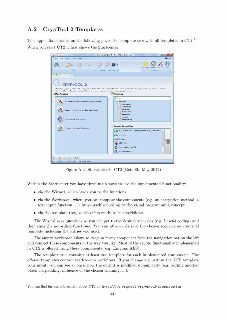
A.2 CrypTool 2 Templates
This appendix contains on the following pages the complete tree with all templates in CT2.2
When you start CT2 it first shows the Startcenter.
Figure A.2: Startcenter in CT2 (Beta 8b, May 2012)
Within the Startcenter you have three main ways to use the implemented functionality:
• via the Wizard, which leads you to the functions.
• via the Workspace, where you can compose the components (e.g. an encryption method, atext input function, ...) by yourself according to the visual programming concept.
• via the template tree, which offers ready-to-run workflows.
The Wizard asks questions so you can get to the desired scenarios (e.g. base64 coding) andthen runs the according functions. You can afterwards save the chosen scenario as a normaltemplate including the entries you used.
The empty workspace allows to drag on it any component from the navigation bar on the leftand connect these components in the way you like. Most of the crypto functionality implementedin CT2 is offered using these components (e.g. Enigma, AES).
The template tree contains at least one template for each implemented component. Theoffered templates contain read-to-run workflows. If you change e.g. within the AES templateyour input, you can see at once, how the output is modified dynamically (e.g. adding anotherblock via padding, influence of the chosen chaining, ...).
2You can find further information about CT2 at: http://www.cryptool.org/en/ct2-documentation
431

Figure A.3: Screenshot of the template tree of CT2 (NB4882.1, July 2012), Part 1
432

A.3 JCrypTool Functions
On the following pages this appendix contains a list of all functions in JCrypTool.3
When you start JCT the first time it shows the Welcome window.
Figure A.4: Welcome screenshot in JCT (RC6, July 2012)
After pressing “Start” you can directly use the different functions. The functions implementedin JCT are presented in two different perspectives:
• Default Perspective
• Algorithm Perspective
All functions of the Default Perspective can be found both in the menus and in thenavigation bar called “Crypto Explorer” (at the right side). The Default Perspective containsall important methods like classic transposition or modern AES, and many visualizations (e.g.Diffie-Hellman key exchange or calculations on elliptic curves).
All functions of the Algorithm Perspective can be found in the navigation bar called“Algorithms” (in this perspective also at the right side). The Algorithm Perspective contains alldetail settings of the various algorithms, it especially offers post-quantum computing algorithms(PQC).
3You can find further information about JCT at: http://www.cryptool.org/en/jct-volunteer
This list was generated using the CT Portal website.
433

Figure A.5: Screenshot of the functions of JCT (RC6, July 2012), Part 1
434

Figure A.6: Screenshot of the functions of JCT (RC6, July 2012), Part 2
435

A.4 CrypTool-Online Functions
This appendix contains a list of all functions in CrypTool-Online (CTO).4
The following screenshot shows the crypto functions implemented on CTO:
4You can find further information about CTO at: www.cryptool-online.org
This list was generated using the functions list at the CT Portal website:https://www.cryptool.org/en/ctp-documentation/ctp-functions
436
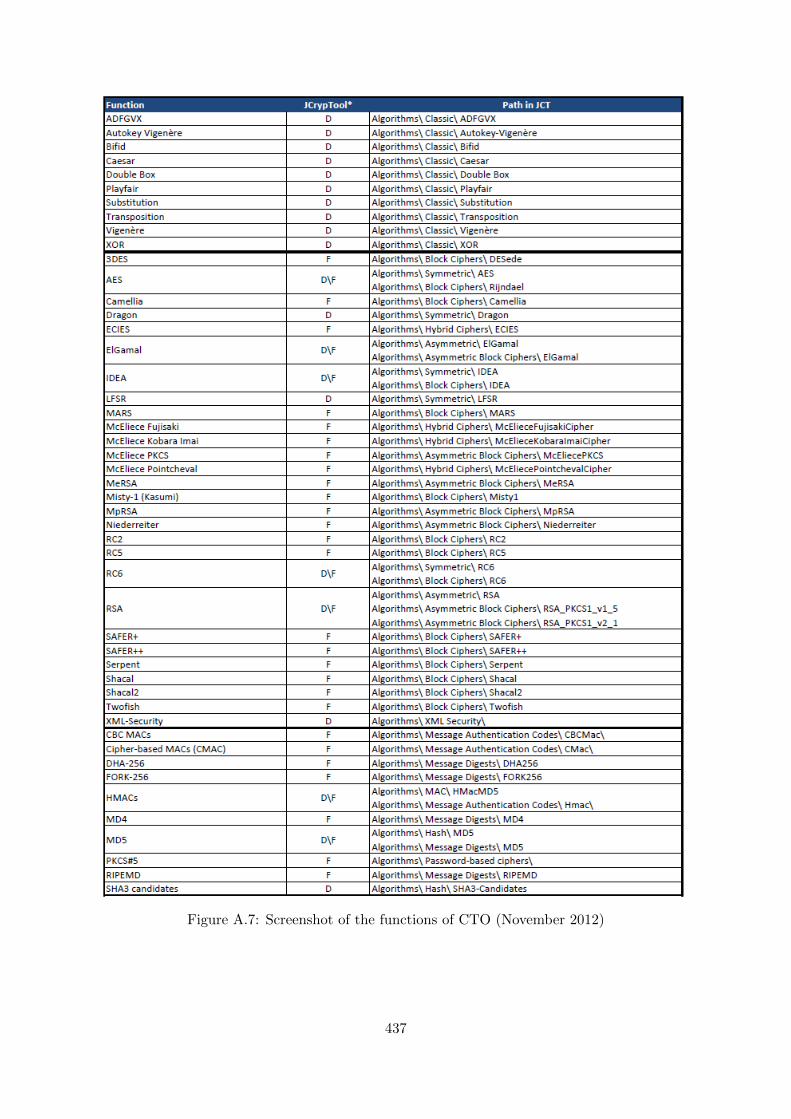
Figure A.7: Screenshot of the functions of CTO (November 2012)
437

A.5 Movies and Fictional Literature with Relation to Cryptog-raphy
Cryptographic applications – classical as well as modern ones – have been used in literature andmovies. In some media they are only mentioned and are a pure admixture; in others they play aprimary role and are explained in detail; and sometimes the purpose of the story, which formsthe framework, is primarily to transport this knowledge and achieve better motivation. Here isthe beginning of an overview.
A.5.1 For Grownups and Teenagers
[Poe1843] Edgar Allan Poe,The Gold Bug, 1843.5
In this short story Poe tells as first-person narrator about his acquaintanceship with thecurious Mr. Legrand. They detect the fabulous treasure of captain Kidd via a gold bugand a vellum found at the coast of New England.The cipher consists of 203 cryptic symbols and it proves to be a general monoalphabeticsubstitution cipher (see chapter 2.2.1). The story tells how they solve the riddle step bystep using a combination of semantic and syntax analysis (frequency analysis of singleletters in English texts).6
In this novel the code breaker Legrand says the famous statement: “Yet it may be roundlyasserted that human ingenuity cannot concoct a cipher which human ingenuity cannotresolve – given the according dedication.”
[Verne1885] Jules Verne,Mathias Sandorf, 1885.This is one of the most famous novels of the French author Jules Verne (1828-1905), whowas called “Father of Science fiction”.In “Mathias Sandorf” he tells the story of the freedom fighter Earl Sandorf, who is betrayedto the police, but finally he can escape.The whistle-blowing worked, because his enemies captured and decrypted a secret messagesent to him. For decryption they needed a special grille, which they stole from him. Thisturning grille was a quadratic piece of jig with 6x6 squares, of which 1/4 (nine) were holes(see the turning grille in chapter 2.1.1).
[Kipling1901] Rudyard Kipling,Kim, 1901.Rob Slade’s review7 of this novel says: “Kipling packed a great deal of information and
5See https://en.wikipedia.org/wiki/The_Gold-Bug.Part 1 of the series RSA & Co. at school: Modern cryptology, old mathematics, and subtle protocols contains a
didactical description for usage at school. Unfortunately this series is currently only available in German. See[WLS98], pp 52 ff (“Das Gold des Gehenkten”).
All material about a gold-bug lesson (double period) can be found at http://www.informatik-im-kontext.de/via “E-Mail (nur?) fur Dich” => “Vertraulichkeit mit Verschlusselungsverfahren”.
Poe not only was a well-known writer, but also a talented cryptographer. His story is also told in the bookCode Breaking [Kip97].
6Part of the learning material above is a Python program which can be used to decrypt the ciphertext with Pythonand with SageMath. See the code example in A.5.3.
7See http://catless.ncl.ac.uk/Risks/24.49.html#subj12.
438

concept into his stories, and in “Kim” we find The Great Game: espionage and spying.Within the first twenty pages we have authentication by something you have, denial ofservice, impersonation, stealth, masquerade, role-based authorization (with ad hoc authen-tication by something you know), eavesdropping, and trust based on data integrity. Lateron we get contingency planning against theft and cryptography with key changes.”The book is out of copyright.8
[Doyle1905] Arthur Conan Doyle,The Adventure of the Dancing Men, 1905.In this Sherlock Holmes short story (first published in 1903 in the “Strand Magazine”, andthen in 1905 in the collection “The Return of Sherlock Holmes” the first time in book-form)Sherlock Holmes has to solve a cipher which at first glance looks like a harmless kid’spicture.But it proves to be the monoalphabetic substitution cipher (see chapter 2.2.1) of thecriminal Abe Slaney. Sherlock Holmes solves the riddle using frequency analysis.
[Sayers1932] Dorothy L. Sayers,Have his carcase, Harper/Victor Gollancz Ltd., 1932.In this novel the writer Harriet Vane finds a dead body at the beach. The police believethe death is suicide. Harriet Vane and the elegant amateur sleuth Lord Peter Wimseytogether clear of the disgusting murder in this second of Sayers’s famous Harriet Vanemystery series.This requires to solve a cryptogram. Surprisingly the novel not only describes the Playfaircipher in detail, but also the cryptanalysis of this cipher (see Playfair in chapter 2.2.3).
[Simmel1970] Johannes Mario Simmel,And Jimmy went to the Rainbow (original title: Und Jimmy ging zum Regenbogen), KnaurVerlag, 1970.The novel plays between 19938 and 1967 in Vienna. The main character Manual Arandauncovers step by step the past of his murdered father. Important for the plot is anencrypted manuscript, which is decrypted in chapter 33. In the novel the cipher is called“25-fold Caesar cipher”. It is actually a Vigenere cipher with a 25 character key.A movie of the novel appeared in 1971.
[Crichton1987] Michael Crichton,Sphere, Pan Books, 1987.A team of different scientists is send to the ground of the ocean in order to investigatea highly developed 900 m long space ship. The human peculiarities and psychologicalproblems of the researchers surface more and more, because of life threatening events andisolation. There are many mysteries: While the space ship lies on the ground for 300 years,it has English markings and a life of its own, and materializing of the researcher’s imagina-tions appear. On a computer screen a cipher text appears, which is completely printed
8You can read it at:http://whitewolf.newcastle.edu.au/words/authors/K/KiplingRudyard/prose/Kim/index.html,http://kipling.thefreelibrary.com/Kim orhttp://www.readprint.com/work-935/Rudyard-Kipling.
439
in the book. The genius mathematician Harry deciphers the simple helical substitution code.
[Seed1990] Directed by Paul Seed,House of Cards, 1990.In this movie Ruth tries to solve the secret, which made her daughter fall silent. Here twoyoung people suffering from autism communicate via 5- and 6-digit primes (see chapter 3).After more than 1 hour the movie contains the following encrypted two series of primes:
21, 383; 176, 081; 18, 199; 113, 933; 150, 377; 304, 523; 113, 933193, 877; 737, 683; 117, 881; 193, 877
[Robinson1992] Directed by Phil Alden Robinson,Sneakers, Universal Pictures Film, 1992.In this movie the “sneakers”, computer experts under their boss Martin Bishop, try toget back the deciphering box SETEC from the “bad guys”. SETEC, invented by a geniusmathematician before he was killed, allows to decrypt all codes from any nation.In the movie the code is not described in any way9.
[Baldacci1997] David Baldacci,Total Control, Mass Market Paperback, 1997.Jason Archer, executive with a technology company suddenly disappears. Sidney Archertries to find out about her husband’s surprising death. She gets a clue how the globalfinancial system is abused and that the real control belongs to those with the most money.Here even good passwords don’t help ...
[Natali1997] Directed by Vincenzo Natali,Cube, Mehra Meh Film, 1997.In this Canadian low-budget-movie 7 complete strangers of widely varying personalitycharacteristics are involuntarily placed in an kafkaesque maze of cubical rooms containingdeadly traps.To get out the persons have to move through these rooms. To find out which roomsare dangerous, mathematics is crucial: Each cubic room has at its entrance a numericalmarking consisting of three sets of three digits. First they deduce that all rooms markedat their entrance with at least one prime number are trapped. Later it comes out that atrapped room can also be marked by a number which is a power of a prime (so traps arepn, e.g. 128 = 27 or 101 = 1011 = prime, but not 517 = 11 ∗ 47).
[Becker1998] Directed by Harold Becker,Mercury Rising, Universal Pictures Film, 1998.The NSA developed a new cipher, which is pretended to be uncrackable by humans andcomputers. To test its reliability some programmers hide a message encrypted with thiscipher in a puzzle magazine.
9Leonard Adleman (the “A” within RSA) worked as mathematical consultant for “Sneakers”. He describes the funnystory about his contribution at his homepage http://www.usc.edu/dept/molecular-science/fm-sneakers.htm.It is assumed that the cipher used everywhere is RSA. According to that within the chip a fast, unknownfactorization method is implemented.
440

Simon, a nine year old autistic boy, cracks the code. Instead of fixing the code, a govern-ment agent sends a killer. FBI agent Art Jeffries (Bruce Willis) protects the boy and setsa snare for the killers.The code is not described in any way.
[Brown1998] Dan Brown,Digital Fortress, E-Book, 1998.Dan Brown’s first novel was published in 1998 as e-book, but it was largely unsuccessfulthen.The National Security Agency (NSA) uses a huge computer, which enables it to decryptall messages (needless to say only of criminals and terrorists) within minutes even if theyuse the most modern encryption methods.An apostate employee invents an unbreakable code and his computer program Diabolusforces the super computer to do self destructing operations. The plot, where also thebeautiful computer expert Susan Fletcher has a role, is rather predictable.The idea, that the NSA or another secret service is able to decrypt any code, is currentlya popular topic. In “Digital Fortress” the super computer has 3 million processors – never-theless from today’s view this is by no means sufficient to hack modern ciphers.
[Elsner1999] Dr. C. Elsner,The Dialogue of the Sisters, c’t, Heise, 1999.In this short story, which is included in the CrypTool package as PDF file, the sistersconfidentially communicate using a variant of RSA (see chapter 4.10 and the following).They are residents of a madhouse being under permanent surveillance.
[Stephenson1999] Neal Stephenson,Cryptonomicon, Harper, 1999.This very thick novel deals with cryptography both in WW2 and today. The two heroesfrom the 40ies are the excellent mathematician and cryptanalyst Lawrence Waterhouse,and the overeager and morphine addicted US marine Bobby Shaftoe. They both aremembers of the special allied unit 2702, which tries to hack the enemy’s communicationcodes and at the same time to hide the own existence.This secretiveness also happens in the present plot, where the grandchildren of the warheroes – the dedicated programmer Randy Waterhouse and the beautiful Amy Shaftoe –team up.Cryptonomicon is notably heavy for non-technical readers in parts. Several pages arespent explaining in detail some of the concepts behind cryptography. Stephenson added adetailed description of the Solitaire cipher (see chapter 2.4), a paper and pencil encryptionalgorithm developed by Bruce Schneier which is called “Pontifex” in the book. Another,modern algorithm called “Arethusa” is not explained in detail.
[Elsner2001] Dr. C. Elsner,The Chinese Labyrinth, c’t, Heise, 2001.In this short story, which is included in the CrypTool package as PDF file, Marco Polo hasto solve problems from number theory within a competition to become a major consultantof the Great Khan. All solutions are included and explained.
441

[Colfer2001] Eoin Colfer,Artemis Fowl, Viking, 2001.In this book for young people the 12 year old Artemis, a genius thief, gets a copy of thetop secret “Book of the Elfs”. After he decrypted it with his computer, he finds out things,men never should have known.The used code is not described in detail or revealed.
[Howard2001] Directed Ron Howard,A Beautiful Mind, 2001.This is the film version of Sylvia Nasar’s biography of the game theorist John Nash. Afterthe brilliant but asocial mathematician accepts secret work in cryptography, his life takesa turn to the nightmarish. His irresistible urge to solve problems becomes a danger forhimself and his family. Nash is – within his belief – a most important hacker working forthe government.Details of his way analysing code are not described in any way.
[Apted2001] Directed by Michael Apted,Enigma, 2001.This is the film version of Robert Harris’ “historical fiction” Enigma (Hutchinson, London,1995) about the World War II code-breaking work at Bletchley Park in early 1943, whenthe actual inventor of the analysis Alan Turing (after Polish pre-work) already was in theUS. So the fictional mathematician Tom Jericho is the lead character in this spy-thriller.Details of his way analysing the code are not described.
[Isau2003] Ralf Isau,The Museum of the stolen memories (original title: Das Museum der gestohlenen Erin-nerungen), Thienemann-Verlag, 1997/2003.In this exciting novel the last part of the oracle can only be solved with the joined help ofthe computer community.The book got several awards and exists in 8 different languages, but not in English yet.
[Brown2003] Dan Brown,The Da Vinci Code, Doubleday, 2003.The director of the Louvre is found murdered in his museum in front of a picture ofLeonardo da Vinci. And the symbol researcher Robert Langdon is involved in a conspiracy.The plot mentions different classic codes (substitution like Caesar or Vigenere, as well astransposition and number codes). Also there are hints about Schneier and the sunflower.The second part of the book contains a lot of theological considerations.This book has become one of the most widely read books of all time.
[Hill2003] Tobias Hill,The Cryptographer, Faber & Faber, 2003.London 2021: The company SoftMark developed and establish an electronic curreny, whichguarantees highest security standards by an unbreakable code. The inventor and companyfounder, called the cryptographer because of his mathematical talent, has become the
442

richest man in the world. But the code was hacked, and in a worldwide economic cri-sis his company goes bankrupt. Additionally the tax investigator Anna Moore is set on him.
[McBain2004] Scott McBain,Final Solution, manuscript not published by Harper Collins, 2004 (German version hasbeen published in 2005).In a near future politicians, chiefs of military and secret services of many different countriestake over all the power. With a giant computer network called “Mother” and completesurveillance they want to cement their power and commercialisation of life forever. Humansare only assessed according to their credit rating and globally acting companies elude ofany democratic control. Within the thriller the obvious injustice, but also the realisticlikelihood of this development are considered again and again.With the help of a cryptographer a code to destroy was built into the super computer“Mother”: In a race several people try to start the deactivation (Lars Pedersen, OswaldPlevy, the female American president, the British prime minister and an unknown Finishnamed Pia, who wants to take revenge for the death of her brother). On the opposite sidea killing group acts under the special guidance of the British foreign minister and the bossof the CIA.
[Preston2005] Douglas Preston,Tyrannosaur Canyon, Forge Books, 2005.A very exciting thriller which also struggles with the question why the dinosaurs died off.
Archeologist Stem Weathers is shot in a canyon. Before his murderer appears he gives hisnotebook to Tom Broadbent, a local animal doctor, coming by accidentally.
The notebook contains on 60 pages only digits. Therefore Tom takes it to Wyman Ford anex-CIA cryptanalyst, who now lives in a nearby abbey, after his wife was killed in action.Wyman first declines and says that self-invented code are “idiot ciphers” – devised by anidiot and easily crackable by each idiot. The notebook then proves to be not that easy.After intensive analysis he finds out that the digits are no code but the output of an earthradar device showing the picture of a well-preserved T.rex.
After around 250 pages of endless chases a surprising turn comes up: Masago, head ofa so-called black-detachment unit of the CIA. He explains: New weapons invented oncealways have been used. Mankind will kill herself, but its his task to postpone that as faras possible. As head of the LS480 department he will prevent by any means possible thatterrorists get any new dangerous biological weapon.
When scanning the dead body of Weathers the murder only found some rock cuttingshe took. These rocks are investigated by a young reseacher named Melody Crookshankalthough she doesn’t know where the rock cuttings come from. She finds within them avery special kind of virus apparently coming from outer-space.
[Burger2006] Wolfgang Burger,Heidelberg Lies (original title: Heidelberger Lugen), Piper, 2006.This detective story playing in the Rhein-Neckar area in Germany has several independentstrands and local stories, but mainly it is about Kriminalrat Gerlach from Heidelberg. Onpage 207 f. the cryptographic reference for one strand is shortly explained: The soldierHorrle had copied circuit diagrams of a new digital NATO decryption device and the
443
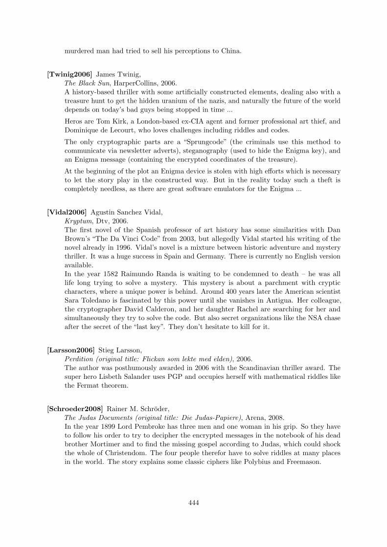
murdered man had tried to sell his perceptions to China.
[Twinig2006] James Twinig,The Black Sun, HarperCollins, 2006.A history-based thriller with some artificially constructed elements, dealing also with atreasure hunt to get the hidden uranium of the nazis, and naturally the future of the worlddepends on today’s bad guys being stopped in time ...
Heros are Tom Kirk, a London-based ex-CIA agent and former professional art thief, andDominique de Lecourt, who loves challenges including riddles and codes.
The only cryptographic parts are a “Sprungcode” (the criminals use this method tocommunicate via newsletter adverts), steganography (used to hide the Enigma key), andan Enigma message (containing the encrypted coordinates of the treasure).
At the beginning of the plot an Enigma device is stolen with high efforts which is necessaryto let the story play in the constructed way. But in the reality today such a theft iscompletely needless, as there are great software emulators for the Enigma ...
[Vidal2006] Agustin Sanchez Vidal,Kryptum, Dtv, 2006.The first novel of the Spanish professor of art history has some similarities with DanBrown’s “The Da Vinci Code” from 2003, but allegedly Vidal started his writing of thenovel already in 1996. Vidal’s novel is a mixture between historic adventure and mysterythriller. It was a huge success in Spain and Germany. There is currently no English versionavailable.In the year 1582 Raimundo Randa is waiting to be condemned to death – he was alllife long trying to solve a mystery. This mystery is about a parchment with crypticcharacters, where a unique power is behind. Around 400 years later the American scientistSara Toledano is fascinated by this power until she vanishes in Antigua. Her colleague,the cryptographer David Calderon, and her daughter Rachel are searching for her andsimultaneously they try to solve the code. But also secret organizations like the NSA chaseafter the secret of the “last key”. They don’t hesitate to kill for it.
[Larsson2006] Stieg Larsson,Perdition (original title: Flickan som lekte med elden), 2006.The author was posthumously awarded in 2006 with the Scandinavian thriller award. Thesuper hero Lisbeth Salander uses PGP and occupies herself with mathematical riddles likethe Fermat theorem.
[Schroeder2008] Rainer M. Schroder,The Judas Documents (original title: Die Judas-Papiere), Arena, 2008.In the year 1899 Lord Pembroke has three men and one woman in his grip. So they haveto follow his order to try to decipher the encrypted messages in the notebook of his deadbrother Mortimer and to find the missing gospel according to Judas, which could shockthe whole of Christendom. The four people therefor have to solve riddles at many placesin the world. The story explains some classic ciphers like Polybius and Freemason.
444
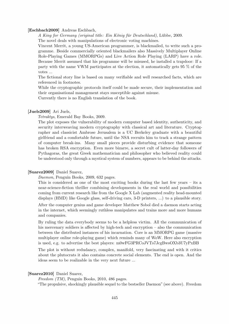
[Eschbach2009] Andreas Eschbach,A King for Germany (original title: Ein Konig fur Deutschland), Lubbe, 2009.The novel deals with manipulations of electronic voting machines.Vincent Merrit, a young US-American programmer, is blackmailed, to write such a pro-gramme. Beside commercially oriented blackmailers also Massively Multiplayer OnlineRole-Playing Games (MMORPGs) and Live Action Role Playing (LARP) have a role.Because Merrit assumed that his programme will be misused, he installed a trapdoor: If aparty with the name VWM participates at the election, it automatically gets 95 % of thevotes ...The fictional story line is based on many verifiable and well researched facts, which arereferenced in footnotes.While the cryptographic protocols itself could be made secure, their implementation andtheir organisational management stays susceptible against misuse.Currently there is no English translation of the book.
[Juels2009] Ari Juels,Tetraktys, Emerald Bay Books, 2009.The plot exposes the vulnerability of modern computer based identity, authenticity, andsecurity interweaving modern cryptography with classical art and literature. Cryptog-rapher and classicist Ambrose Jerusalem is a UC Berkeley graduate with a beautifulgirlfriend and a comfortable future, until the NSA recruits him to track a strange patternof computer break-ins. Many small pieces provide disturbing evidence that someonehas broken RSA encryption. Even more bizarre, a secret cult of latter-day followers ofPythagoras, the great Greek mathematician and philosopher who believed reality couldbe understood only through a mystical system of numbers, appears to be behind the attacks.
[Suarez2009] Daniel Suarez,Daemon, Penguin Books, 2009, 632 pages.This is considered as one of the most exciting books during the last few years – its anear-science-fiction thriller combining developments in the real world and possibilitiescoming from current research like from the Google X Lab (augmented reality head-mounteddisplays (HMD) like Google glass, self-driving cars, 3-D printers, ...) to a plausible story.
After the computer genius and game developer Matthew Sobol died a daemon starts actingin the internet, which seemingly ruthless manipulates and trains more and more humansand companies.
By ruling the data everybody seems to be a helpless victim. All the communication ofhis mercenary soldiers is affected by high-tech and encryption – also the communicationbetween the distributed instances of his incarnation. Core is an MMORPG game (massivemultiplayer online role-playing game) which reminds many of WoW. Here also encryptionis used, e.g. to advertise the best players: m0wFG3PRCoJVTs7JcgBwsOXb3U7yPxBB
The plot is without redudancy, complex, manifold, very fascinating and with it criticsabout the plutocrats it also contains concrete social elements. The end is open. And theideas seem to be realizable in the very next future ...
[Suarez2010] Daniel Suarez,Freedom (TM), Penguin Books, 2010, 486 pages.“The propulsive, shockingly plausible sequel to the bestseller Daemon”(see above). Freedom
445

(TM) (Daemon #2) patches a number of holes the writer left in the first book. The proseis tighter, the descriptions more direct, the characters are fleshed out, especially Loki.Having laid the groundwork in “Daemon”, Suarez uses this foundation in order to explorea new concept of social organization based on empowering information technology andthe reasoning why and how the battle runs between the old potentates and the Daemonsociety, which also evolves further already during the story. Cryptography is a naturalpart of modern technology and modern warfare as described in this book. The new societyemerging in “Freedom (TM)” is based on the darknet, an alternative to the internet usingfast wireless meshes in order to increase the durability and availability of the network.Despite the story is shocking in some parts, it appears to be realistic and not far awayfrom the parallel usage of modern technology integrated into our modern lives as a virtualworld overlaying our real world.
[Olsberg2011] Karl Olsberg,Rafael 2.0 (original title: Rafael 2.0), Thienemann Verlag, 2011, 240 pages.Michael and Rafael Ogilvy are talented twins who get along very well. Before the terminallyill Rafael dies, his father developed a virtual computer effigy of him, an artificial intelligence(AI). This is a good kept secret until Michael one day finds out what his father is hidingbefore him. However, his first horror soon turns into joy. So he still has something thatreminds him of his brother.But this computer system is also interesting for the military. One day Michael’s father iskidnapped and the company and thus also the computer program Rafael 2.0 fall into thewrong hands. Michael is banished by his uncle in a boarding school, from which he canflee. Henceforth, Michael and his friends try their best to find his father, of whom theyassume that he was abducted by a competing company. From here the story gets reallyexciting ... Michael learns that there is another artificial intelligence, Metraton, which isnot so well-disposed to the people. Nothing is too much engrossed, young teenagers arethe target audience. Nevertheless, depth and substance are created when for instance themachinations in acquisitions are discussed.From a crypto perspective,the section about factoring is thrilling: With a variant Michaelcan detect whether the computer is cheating ...
[Burger2011] Wolfgang Burger,The fifth murderer (original title: Der funfte Morder), Piper, 2011.Location & time of the story: Germany / Heidelberg, 1990 - 2009. Episode 7 of theAlexander-Gerlach series. Inspector Alexander Gerlach became almost a victim of a bombblast when the sport utility vehicle (SUV) of a Bulgarian panderer exploded. Gerlach startsinvestigating because he wants to prevent a gang warfare, but then his bosses call him off.When the journalist Machatschek supports Gerlach, he communicates with him only viaSkype using an add-on encryption program which he believes is the most secure in the world.
[Eschbach2011] Andreas Eschbach,Master of the universe – master of all staff (original title: Herr aller Dinge), Lubbe, 2011.This novel would have deserved a much broader audience: The idea in it of the “mostterrific of all crimes”, which is the origin of the whole story, is new and almost revolutionary,but also infinitely sad. Along the failing partnership of Hiroshi (inventor genius) andCharlotte important topics like justice, human wealth and power are dealt with.
446
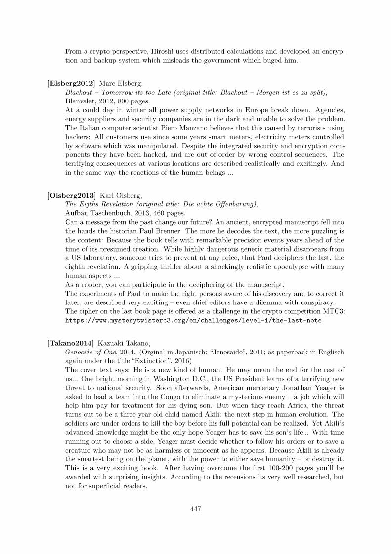
From a crypto perspective, Hiroshi uses distributed calculations and developed an encryp-tion and backup system which misleads the government which buged him.
[Elsberg2012] Marc Elsberg,Blackout – Tomorrow its too Late (original title: Blackout – Morgen ist es zu spat),Blanvalet, 2012, 800 pages.At a could day in winter all power supply networks in Europe break down. Agencies,energy suppliers and security companies are in the dark and unable to solve the problem.The Italian computer scientist Piero Manzano believes that this caused by terrorists usinghackers: All customers use since some years smart meters, electricity meters controlledby software which was manipulated. Despite the integrated security and encryption com-ponents they have been hacked, and are out of order by wrong control sequences. Theterrifying consequences at various locations are described realistically and excitingly. Andin the same way the reactions of the human beings ...
[Olsberg2013] Karl Olsberg,The Eigths Revelation (original title: Die achte Offenbarung),Aufbau Taschenbuch, 2013, 460 pages.Can a message from the past change our future? An ancient, encrypted manuscript fell intothe hands the historian Paul Brenner. The more he decodes the text, the more puzzling isthe content: Because the book tells with remarkable precision events years ahead of thetime of its presumed creation. While highly dangerous genetic material disappears froma US laboratory, someone tries to prevent at any price, that Paul deciphers the last, theeighth revelation. A gripping thriller about a shockingly realistic apocalypse with manyhuman aspects ...As a reader, you can participate in the deciphering of the manuscript.The experiments of Paul to make the right persons aware of his discovery and to correct itlater, are described very exciting – even chief editors have a dilemma with conspiracy.The cipher on the last book page is offered as a challenge in the crypto competition MTC3:https://www.mysterytwisterc3.org/en/challenges/level-i/the-last-note
[Takano2014] Kazuaki Takano,Genocide of One, 2014. (Orginal in Japanisch: “Jenosaido”, 2011; as paperback in Englischagain under the title “Extinction”, 2016)The cover text says: He is a new kind of human. He may mean the end for the rest ofus... One bright morning in Washington D.C., the US President learns of a terrifying newthreat to national security. Soon afterwards, American mercenary Jonathan Yeager isasked to lead a team into the Congo to eliminate a mysterious enemy – a job which willhelp him pay for treatment for his dying son. But when they reach Africa, the threatturns out to be a three-year-old child named Akili: the next step in human evolution. Thesoldiers are under orders to kill the boy before his full potential can be realized. Yet Akili’sadvanced knowledge might be the only hope Yeager has to save his son’s life... With timerunning out to choose a side, Yeager must decide whether to follow his orders or to save acreature who may not be as harmless or innocent as he appears. Because Akili is alreadythe smartest being on the planet, with the power to either save humanity – or destroy it.This is a very exciting book. After having overcome the first 100-200 pages you’ll beawarded with surprising insights. According to the recensions its very well researched, butnot for superficial readers.
447

From a crypto perspective, RSA and OTP are directly drivers of the story and are explainedcorrectly. Breaking RSA by factorization is so important that the CIA wouldn’t acceptthat this knowledge isn’t in their ownership ...
[Elsberg2014] Marc Elsberg,ZERO – They Know what you are Doing (original title: ZERO – Sie wissen, was du tust),Blanvalet Verlag, 2014, 480 pages.London. In a pursuit a boy is shot. His death takes the journalist Cynthia Bonsant tothe acclaimed internet platform Freemee. Freemee collects and analyzes data, and thuspromises its millions of users – rightly – a better life and more success. There is only onewho warns about Freemee and about the power that the online newcomer could give just afew: ZERO, the most searched online activist in the world. As Cynthia begins precisely toresearch, she’s becoming the quarry. And in a world of cameras, headsets and smartphonesthere is no escape ...Highly topical and menacing: the transparent person under control. The novel takesplace in the near future (near fiction) and contains many contemporary references such asPRISM, predictive analytics, gamification. By the way, references to well-known sciencefiction media like “The Running Man”, “Monkey Wrench Gang”, “V as Vendetta” (V wearsa Guy Fawkes mask, now the hallmark of Anonymous), “Network” and “Body Snatchers”are processed.Technologically / cryptologically the protagonists move on the highest level, which is notfurther explained: Alice Kinkaid communicates with a Raspberry Pi. Cynthia’s daughterVi uses mesh networks. Seehttps://de.wikipedia.org/wiki/Zero_%E2%80%93_Sie_wissen,_was_du_tust,http://www.zero-das-buch.de/actiontrailer.php
[Lagercrantz2015] David Lagercrantz,The Girl in the Spider’s Web, Quercus, 2015.This is the 4th novel in the Millennium series, and the first not written by Stieg Larsson.While Mikael Blomkvist’s print medium is struggling to survive the reader gets more andmore insight in the inner structures and the combinations of publishers, secret services,public agencies, organized crime, and industrial espionage. Here, no care is taken for singlehumans, and normal humans would have no chance aginst this mix of interests. However,the special skills of Lisbeth Salander makes a difference, and so the NSA is informed, thatparts of it are led and misused by organized crime. The characters of the Millenium trilogyhave been developed further in a credible way. Very exiting.From a crypto perspective, Lisbeth and the autist August deal with elliptic curves to crackRSA.See https://en.wikipedia.org/wiki/The_Girl_in_the_Spider%27s_Web.
Remark 1: A long list of (partly commented) samples of cryptology in fictional literature canbe found on the following German web page:http://www.staff.uni-mainz.de/pommeren/Kryptologie/Klassisch/0_Unterhaltung/
For some older authors (e.g. Jules Verne, Karl May, Arthur Conan Doyle, Edgar Allen Poe)there are links to the original and relevant text pieces.
448

Remark 2: You can find title pages of some of these books on the web site of Tobias Schrodel,who collects classic books about cryptography:
http://tobiasschroedel.com/crypto_books.php
Remark 3: If you know of further books and movies, where cryptography has a major rolethen we would be very glad if you could send us the exact title and a short explanation aboutthe movie/book’s content. We will insinuate your possible enthusiasm for a title. Thanks a lot.
449

A.5.2 For Kids and Teenagers
The following list contains movies and “kid books”. The kid books contain both stories, andcollections of simple ciphers, prepared in a didactic and exciting manner (please send us similarEnglish kid books and kid movies, because at the moment our list contains mostly German kidbooks):
[Mosesxxxx] [no named author],Top secret – The Book for Detectives and Spies (original title: Streng geheim – Das Buchfur Detektive und Agenten), Edition moses, [no year named].This is a thin book for small kids with Inspector Fox and Dr. Chicken.
[Arthur196x] Robert Arthur,The Three Investigators: The Secret Key (German version: Die 3 ???: Der geheimeSchlussel nach Alfred Hitchcock (volume 119), Kosmos-Verlag (from 1960)The three detectives Justus, Peter and Bob have to decrypt covered and encrypted messageswithin this story to find out what is behind the toys of the Copperfield company.
[Para1988] Para,Ciphers (original title: Geheimschriften), Ravensburger Taschenbuch Verlag, 1988 (1stedition 1977).On 125 pages filled with a small font this mini format book explains many methods whichyoung children can apply directly to encrypt or hide their messages. A little glossary and ashort overview about the usage of encryption methods in history complete this little book.
Right at page 6 it summarizes for beginners in an old fashion style “The Important ThingsFirst” about paper&pencil encryption (compare chapter 2):
- “It must be possible to encrypt your messages at any place and at any location withthe easiest measures and a small effort in a short time.
- Your cipher must be easy to remember and easy to read for your partners. Butstrangers should not be able to decrypt them.Remember: Fastness before finesse, security before carelessness.
- Your message must always be as short and precise as a telegram. Shortness outranksgrammar and spelling. Get rid of all needless like salutations or punctuation marks.Preferably use only small or only capital letters.”
[Muller-Michaelis2002] Matthias Muller-Michaelis,The manual for detectives. Everything you need to know about ciphers, codes, readingtracks and the biggest detectives of the world (original title: Das Handbuch fur Detektive.Alles uber Geheimsprachen, Codes, Spurenlesen und die großen Detektive dieser Welt),Sudwest, 2002.
[Kippenhahn2002] Rudolf Kippenhahn,Top secret! – How to encrypt messages and to hack codes (original title: Streng geheim! –Wie man Botschaften verschlusselt und Zahlencodes knackt), rororo, 2002.In this novel a grandpa, an expert for secret writings teaches his four grandchildren and
450

their friends, how to encrypt messages which nobody should read. Because there is some-one who hacks their secrets, the grandpa has to teach them more and more complicatedmethods.Within this story, which forms the framework, the most important classic encryptionmethods and its analysis are explained in a manner exciting and appropriate for children.
[Harder2003] Corinna Harder and Jens Schumacher,Top secret. The big book for detectives (original title: Streng geheim. Das große Buch derDetektive), Moses, 2003.
[Talke-Baisch2003] Helga Talke and Milena Baisch,Your mission in the weird villa. Riddle thriller (original title: Dein Auftrag in der unheim-lichen Villa. Kennwort Ratselkrimi), Loewe, 2003.From 4th form, http://www.antolin.de
Young detectives are faced simple ciphers and codes during their missions.
[Flessner2004] Bernd Flessner,The Three Investigators: Manual for Secret Messages (original title: Die 3 ???: HandbuchGeheimbotschaften), Kosmos, 2004.On 127 pages you learn in an easy and exciting manner, structured by the method types,which secret languages (like the one of the Navajo Indians or dialects) and which secretwritings (real encryption or hiding via technical or linguistic steganography) existed andhow simple methods can be decrypted.The author tells where in history the methods were used and in which novel authors usedencryption methods [like in Edgar Allan Poe’s “The Gold Bug”, like with Jules Verne’shero Mathias Sandorf or like with Astrid Lindgren’s master detective Blomquist who usedthe ROR language (similar inserting ciphers are the spoon or the B language)].This is a didactically excellent introduction for younger teens.
[Zubert2005] Directed by Christian Zubert,The Treasure of the White Hawks (original title: Der Schatz der weißen Falken) , 2005.This exciting adventure movie for kids ties in with the tradition of classics like “TomSawyer and Huckleberry Finn” or Enid Blytons “Five Friendse”. The plot happens insummer 1981. In an old half tumbledown villa three young kids find the treasure map ofthe “White Hawks”, which they decrypt with the help of a computer. Traced by anothergang they aim to go to an old castle.
[Dittert2011] Christoph Dittert,The Three Investigators: Secret Messages (German version: Die 3 ???: GeheimnisvolleBotschaften) (volume 160), Kosmos, 2011In the house of Professor Mathewson an old hand-made book was stolen. The threedetectives Justus, Peter and Bob are getting attacked by a ruthless opponent, who seemsto be always a step ahead. A major part in this story is played by a palimpsest, an ancientmanuscript page, written upon newly. Using X-rays they can make visible again the oldtext below. Its not only the story which is exciting, but also the way, how the instructionfor a treasure hunt is encrypted. Despite using the simple railfence cipher it’s not easy
451

to solve it, as the message is distributed onto two slips and as the printed symbols don’tmean single letters.
Remark 1: You can find title pages of many of these kid books on the web site of TobiasSchrodel, who collects classic books about cryptography:
http://tobiasschroedel.com/crypto_books.php
Remark 2: If you know of further books, which address cryptography in a didactic and forchildren adequate way, then we would be very glad if you could send us the exact book title anda short explanation about the book’s content. Thanks a lot.
452

A.5.3 Code for the light fiction books
Chapter A.5.1 lists as first book “The Gold Bug” by E.A. Poe.
Using the following Python code10 you can decrypt the ciphertext of Captain Kidd (see theoriginal text of “The Gold Bug” in http://pinkmonkey.com/dl/library1/gold.pdf, page 21)with Python or with SageMath.
The code already contains the ascii characters of the ciphertext and the correlated alphabetsfor the plaintext and the ciphertext of this monoalphabetic cipher.
The easiest way to perform the decryption is using the SageMathCell server (http://sagecell.sagemath.org/) in a browser: There you can switch between the programming languagesSage and Python. The code can be executed by insering it with “copy and paste” and thenpressing “Evaluate”.
SageMath sample A.1 Decryption of the Gold-Bug ciphertext from the novel of E.A. Poe(with Python)
# Hier geht’s los ... Start here
import string
PA = ’ETHSONAIRDGLBVPFYMUC’
print ’Plaintext alphabet PA: ’, PA, ’ Length of PA’, len(PA)
CA = "8;4)+*56(!302’.1:9?-"
print ’Ciphertext alphabet CA: ’, CA, ’ Length of CA’, len(CA)
codetableC2P = string.maketrans(CA,PA)
C = ’’’53++!305))6*;4826)4+.)4+);806*;48!8’60))85;1+(;:+*8!83(88)5*!;46
(;88*96*?;8)*+(;485);5*!2:*+(;4956*2(5*-4)8’8*;4069285);)6!8)4++;1(+9;4
8081;8:8+1;48!85;4)485!528806*81(+9;48;(88;4(+?34;48)4+;161;:188;+?;’’’
P = string.translate(C, codetableC2P);
print ’Kidd decrypted:’, P
# ... und hier sind wir schon fertig ... and here we are done!
Remark 1: When printing the ciphertext of Poe, Pinkmonkey “cheated” similarly like thecode author by using only ascii characters.
In the archive of an original publication (e.g. at https://archive.org/details/goldbu
g00poegoog at page 95) you can see, that Poe used characters which were common in theletterpress printing (and most of them are also part of the ascii set). It is very unlikely that anuntaught pirate would use just such characters for his ciphertext ...
Remark 2: The code uses the Python functions “maketrans” und “translate” from the Stringpackage (see e.g. the Python 2.7 documentation, section “functions”).
So both alphabets (for the plaintext and the ciphertext) are inserted as a simple string, and“maketrans” creates a mapping table. The actual encryption is done by “translate”. For thedecryption you just have to switch the arguments of “maketrans” for the two alphabets. Theotherwise necessary transformations between characters and their ascii numbers (using “str” and“ord”) can be avoided. This is ideal for monoalphabetic ciphers – especially for lessons at thejunior high school.
10See [WLS98] and the file 2_MonoKidd.zip at http://bscw.schule.de/pub/bscw.cgi/159132.
453

Remark 3: The following screenshot shows the execution of the Python code on the Sage-MathCell server (http://sagecell.sagemath.org/).
SageMathCell is the browser interface for Sage. Its functions are delivered for free on theSage cell server (Sage is a comprehensive open-source math software system).
Figure A.8: Usage of SageMathCell to decipher Poe’s Gold Bug (with Python)
As result we get:
Plaintext alphabet PA: ETHSONAIRDGLBVPFYMUC Length of PA 20
Ciphertext alphabet CA: 8;4)+*56(!302’.1:9?- Length of CA 20
Kidd decrypted: AGOODGLASSINTHEBISHOPSHOSTELINTHEDEVILSSEATFORTYONEDEGREES
ANDTHIRTEENMINUTESNORTHEASTANDBYNORTHMAINBRANCHSEVENTHLIMB
EASTSIDESHOOTFROMTHELEFTEYEOFTHEDEATHSHEADABEELINEFROMTHE
TREETHROUGHTHESHOTFIFTYFEETOUT
It’s evident how less code is needed with Python or Sage for such tasks. In the above samplethere were 2 unnecessary comment lines, 3 lines for input, 3 lines of real code, and 3 lines for theoutput; really necessary were only 7 lines of code.
454

A.6 Learning Tool for Elementary Number Theory
CT1 contains an interactive educational tool for elementary number theory, called “NT”.11
The educational tool “NT” (number theory) by Martin Ramberger introduces number theoryand visualizes many of the methods and concepts. Where necessary it show the accordingmathematical formulas. Often you can apply the mathematical methods dynamically with yourown small numerical examples.
The content of this educational tool is mainly based on the books by J. Buchmann and H.Scheid [Buc16, Sch06].
This visualized educational tool was build with Authorware 4.12
Request for enhancement/upgrade: It would be desirable to update it to a new versionAuthorware or to use another development platform. If there are developers interested to dothis, I’d be more than happy (please send an email at the author of this CrypTool script).
Figures: The figures A.9 till A.16 give you an impression of the educational tool “NT”:
Figure A.9: Each common divisor of two integers also divides all its linear combinations
11NT can be called in CT1 via the menu path Indiv. Procedures \ Number Theory Interactive \ LearningTool for Number Theory.
12As Authorware is outdated and as the vendor didn’t make tools available to easily port it to his successor products,the program ZT will not be further developed.
455

Figure A.10: Euklid’s algorithm to determine gcd
Figure A.11: Distribution of primes and its differences
456
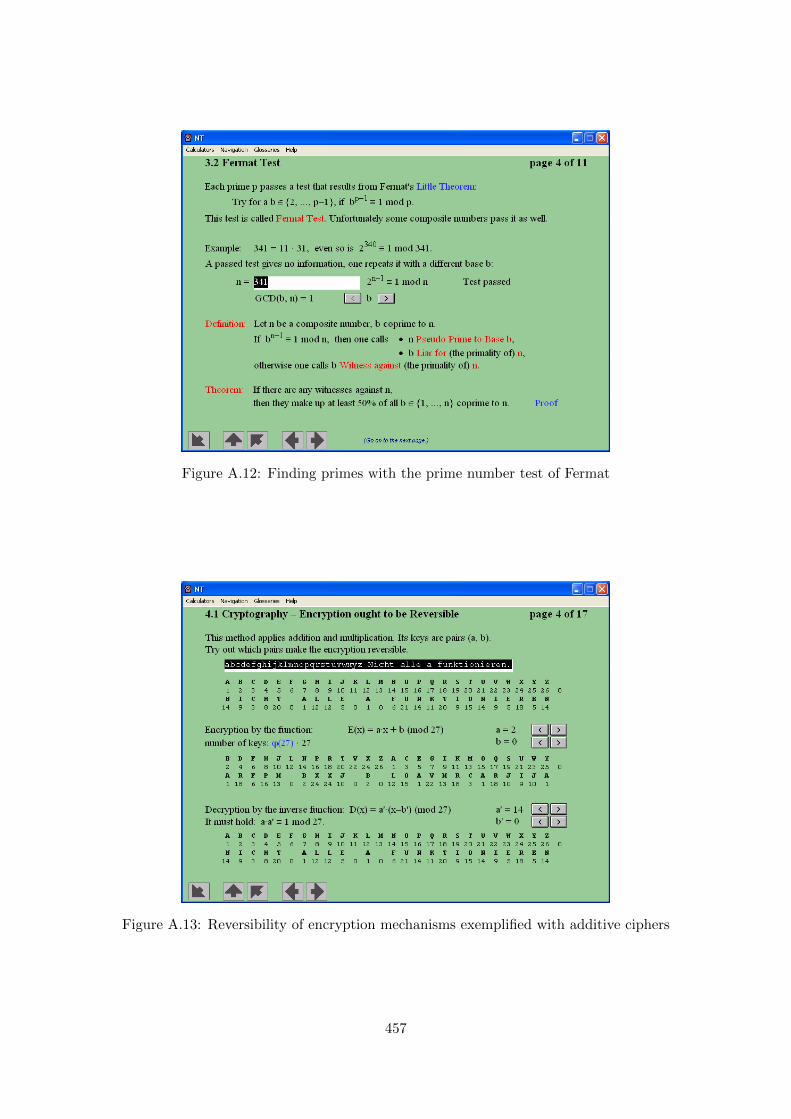
Figure A.12: Finding primes with the prime number test of Fermat
Figure A.13: Reversibility of encryption mechanisms exemplified with additive ciphers
457

Figure A.14: Fermat factorization using the third binomial formula
Figure A.15: Fermat factorization: detecting squares
458

Figure A.16: Pollard’s rho factorization: Floyd’s cycle finding algorithm
459

Bibliography (Appendix LearnTool)
[Buc16] Buchmann, Johannes: Einfuhrung in die Kryptographie. Springer, 6th edition, 2016.Paperback.
[Kip97] Kippenhahn, Rudolf: Verschlusselte Botschaften: Geheimschrift, Enigma und Chipkarte.rowohlt, 1st edition, 1997. New edition 2012, Paperback, Verschlusselte Botschaften:Geheimschrift, Enigma und digitale Codes.
[Sch06] Scheid, Harald: Zahlentheorie. Spektrum Akademischer Verlag, 4th edition, 2006.
[WLS98] Witten, Helmut, Irmgard Letzner, and Ralph Hardo Schulz: RSA & Co. in der Schule:Moderne Kryptologie, alte Mathematik, raffinierte Protokolle, Teil 1: Sprache undStatistik. LOG IN, 1998(3/4):57–65, 1998.http://bscw.schule.de/pub/bscw.cgi/d637160/RSA_u_Co_T1.pdf.
460

A.7 Short Introduction into the CAS SageMath
This book includes numerous code samples using SageMath. SageMath is an open sourcecomputer algebra system (CAS) that supports teaching, study and research in mathematics. Itcombines many high-quality open source packages13 and provides access to their functionalitiesvia a common interface, namely, a Python14 based programming language.
SageMath can be used as a powerful desktop calculator, as a tool to help (undergraduate)students study mathematics, or as a programming environment for prototyping algorithms andresearch in algorithmic aspects of mathematics.
You can get a quick impression of SageMath e.g. with the references in this footnote15.
The official SageMath online documentation16 is available at: http://www.sagemath.org.
In the meantime there are lots of PDF and HTML documents about using SageMath, so wename only a few of them as a good starting point17.
With respect to studying cryptography, SageMath modules can be used to complement a firstcourse in cryptography18.
Comprehensive introductions into cryptography are in this footnote19.
SageMath user interfaces
SageMath is available free of charge and can be downloaded from the following website:
http://www.sagemath.org
13To get an impression of how big SageMath is: After downloading the source of SageMath 4.1, it took around 5hours on an average Linux PC to compile the whole system including all libraries. The compiled version occupied1.8 GB disk space.
14There is also an easy interface to the C language, called Cython, which can be used to substantially speed upfunctions in SageMath.See http://openwetware.org/wiki/Open_writing_projects/Sage_and_cython_a_brief_introduction.
15- “Invitation to Sage” by David Joyner, last update 2009http://sage.math.washington.edu/home/wdj/teaching/calc1-sage/an-invitation-to-sage.pdf
- “The SDSU Sage Tutorial”,http://www-rohan.sdsu.edu/~mosulliv/sagetutorial/
http://www-rohan.sdsu.edu/~mosulliv/sagetutorial/sagecalc.html
- “SAGE For Newbies” by Ted Kosan, 2007,http://sage.math.washington.edu/home/tkosan/newbies_book/sage_for_newbies_v1.23.pdf
16The corresponding official PDF documents can be downloaded athttp://www.sagemath.org/help.html, http://www.sagemath.org/doc and http://planet.sagemath.org.
17- “Library”: http://www.sagemath.org/library/index.html,- “Documentation Project”: http://wiki.sagemath.org/DocumentationProject,- “Teaching”: http://wiki.sagemath.org/Teaching_with_SAGE.
18- Module sources in the directory SAGE_ROOT/devel/sage-main/sage/crypto.- Overview, what crypto currently is in SageMath:http://www.sagemath.org/doc/reference/sage/crypto/
- Discussions about teaching related aspects of development crypto in SageMath:http://groups.google.com/group/sage-devel/browse_thread/thread/c5572c4d8d42d081
19- David Kohel’s notes from 2008 are a ready courcehttp://www.sagemath.org/library/crypto.pdf or the same eventually newer athttp://sage.math.washington.edu/home/wdj/teaching/kohel-crypto.pdf .- “Introduction to Cryptography with Open-Source Software, a very good book from Alasdair McAndrew, CRC,2011
461

The default interface to SageMath is command line based, as shown in figure A.17. However,there is a graphical user interface to the software as well in the form of the SageMath notebook(see figure A.18). We can even use SageMath notebooks20 online at different servers, withouthaving to install SageMath locally, e.g:
http://www.sagenb.org orhttp://sage.mathematik.uni-siegen.de:8000
SageMath runs under many Linux distributions, Mac OS X, and Windows. For the Windowsplatform, a complete distribution of SageMath currently only runs as a VMware image.
Figure A.17: SageMath command line interface
20Further details about SageMath notebooks can be found at chapter 7.9.2 (“Implementing elliptic curves foreducational purposes”⇒ “SageMath”).
21To start the SageMath gui locally: Enter notebook() at the SageMath prompt, and then your favorite browser(Iceweasel, Firefox, IE, ...) is started e.g. with the URL http://localhost:8000.
462

Figure A.18: SageMath notebook interface21
Getting help with using SageMath
Upon loading SageMath from the command line, we are presented with something similar to thefollowing:
mnemonic:~$ sage
----------------------------------------------------------------------
| Sage Version 4.1, Release Date: 2009-07-09 |
| Type notebook() for the GUI, and license() for information. |
----------------------------------------------------------------------
sage: help
Type help() for interactive help, or help(object) for help about object.
sage:
sage:
sage: help()
Welcome to Python 2.6! This is the online help utility.
If this is your first time using Python, you should definitely check out
the tutorial on the Internet at http://docs.python.org/tutorial/.
Enter the name of any module, keyword, or topic to get help on writing
Python programs and using Python modules. To quit this help utility and
return to the interpreter, just type "quit".
To get a list of available modules, keywords, or topics, type "modules",
"keywords", or "topics". Each module also comes with a one-line summary
463

of what it does; to list the modules whose summaries contain a given word
such as "spam", type "modules spam".
Plenty of help is provided in the form of the official SageMath documentation that is distributedwith every release of SageMath (see Figure A.19). The official SageMath standard documentation
Figure A.19: The SageMath standard documentation
includes the following documents:
• Tutorial — This tutorial is designed to help SageMath beginners become familiar withSageMath. It covers many features that beginners should be familiar with, and takes oneto three hours to go through.
• Constructions — This document is in the style of a SageMath “cookbook”. It is a collectionof answers to questions about constructing various objects in SageMath.
• Developers’ Guide — This guide is for developers who want to contribute to the developmentof SageMath. Among other issues, it covers coding style and conventions, modifying thecore SageMath libraries, modifying the SageMath standard documentation, and codereview and distribution.
• Reference Manual — This manual provides complete documentation on the major featuresof SageMath. The description of a class is accompanied by numerous code samples. Allcode samples in the reference manual are tested before each SageMath release.
• Installation Guide — This guide explains how to install SageMath under various platforms.
464

• A Tour of Sage — This is a tour of SageMath that showcases various features of SageMaththat are useful for beginners.
• Numerical Sage — This document introduces tools available under SageMath that areuseful for numerical computation.
• Three Lectures about Explicit Methods in Number Theory Using Sage — This documentis about using SageMath to perform computations in advanced number theory.
From within a SageMath session, we can obtain a list of commands matching some pattern. Todo so, we type the first few characters and then press the “Tab” key:
sage: Su[TAB]
Subsets Subwords SuzukiGroup
SubstitutionCryptosystem SupersingularModule
If we know the exact name of a command, we can use the help function to obtain furtherinformation on that command, or append the question mark “?” to the command name. Forexample, the command help(SubstitutionCryptosystem) provides documentation on thebuilt-in class SubstitutionCryptosystem. We can get documentation on this class with thequestion mark as follows:
sage: SubstitutionCryptosystem?
Type:type
Base Class:<type ’type’>
String Form:<class ’sage.crypto.classical.SubstitutionCryptosystem’>
Namespace:Interactive
File:/home/mvngu/usr/bin/sage-3.4.1/local/lib/python2.5/site-packages/sage/crypto/classical.py
Docstring:
Create a substitution cryptosystem.
INPUT:
- ‘‘S‘‘ - a string monoid over some alphabet
OUTPUT:
- A substitution cryptosystem over the alphabet ‘‘S‘‘.
EXAMPLES::
sage: M = AlphabeticStrings()
sage: E = SubstitutionCryptosystem(M)
sage: E
Substitution cryptosystem on Free alphabetic string monoid
on A-Z
sage: K = M([ 25-i for i in range(26) ])
sage: K
ZYXWVUTSRQPONMLKJIHGFEDCBA
sage: e = E(K)
sage: m = M(‘‘THECATINTHEHAT’’)
sage: e(m)
GSVXZGRMGSVSZG
TESTS::
sage: M = AlphabeticStrings()
465

sage: E = SubstitutionCryptosystem(M)
sage: E == loads(dumps(E))
True
For further assistance on specific problems, we can also search the archive of the sage-support
mailing list at
http://groups.google.com/group/sage-support
466

Examples using the built-in mathematical functions in SageMath
Here are a few little examples22 (all in console mode, for ease) to see what you can do withSageMath:
SageMath sample A.2 Some small general samples in SageMath from different areas inmathematics# * Calculus:
sage: x=var(’x’)
sage: p=diff(exp(x^2),x,10)*exp(-x^2)
sage: p.simplify_exp()
1024 x^10 + 23040 x^8 + 161280 x^6 + 403200 x^4 + 302400 x^2 + 30240
# * Linear Algebra:
sage: M=matrix([[1,2,3],[4,5,6],[7,8,10]])
sage: c=random_matrix(ZZ,3,1);c
[ 7 ]
[-2 ]
[-2 ]
sage: b=M*c
sage: M^-1*b
[ 7 ]
[-2 ]
[-2 ]
# * Number theory:
sage: p=next_prime(randint(2^49,2^50));p
1022095718672689
sage: r=primitive_root(p);r
7
sage: pl=log(mod(10^15,p),r);pl
1004868498084144
sage: mod(r,p)^pl
1000000000000000
# * Finite Fields (\url{http://en.wikipedia.org/wiki/Finite_field}):
sage: F.<x>=GF(2)[]
sage: G.<a>=GF(2^4,name=’a’,modulus=x^4+x+1)
sage: a^2/(a^2+1)
a^3 + a
sage: a^100
a^2 + a + 1
sage: log(a^2,a^3+1)
13
sage: (a^3+1)^13
a^2
22The examples are from the blog of Dr. Alasdair McAndrew, Victoria University,http://amca01.wordpress.com/2008/12/19/sage-an-open-source-mathematics-software-system
467

Writing code samples with SageMath
When you start using a CAS (computer algebra system) you normally type in the single commandson the command line as in the above example23.
But if you develop your own functions, modify them and call them, then it is much easierto do the development in your own editor, save it to a script file and execute the functionsnon-interactively on the command line manually. Both ways to develop code were appliedin chapter 1.8 (“Appendix: Examples using SageMath”), chapter 2.5 (“Appendix: Examplesusing SageMath”), chapter 3.14 (“Appendix: Examples using SageMath”) and in chapter 4.19(“Appendix: Examples using SageMath”).
To program and test SageMath code using an editor there are two useful commands: load()
and attach()24.Suppose you have a function definition like this:
def function(var1):
r"""
DocText.
"""
...
return (L)
which has been saved to the file primroots.sage.
To load this function into SageMath (and do a syntax check at once), use load() as follows:
sage: load primroots.sage
and you can then proceed to use on the command line any variable or function defined in thatSageMath script25.
Normally we also want to edit our own SageMath script and reload the content of the changedscript into SageMath again. In that case, you can use the command attach() (you also canapply attach() directly after loading the script, even before having changed the script; and youcan even omit load(), as this is contained in attach()):
23The standard way for presenting SageMath code starts the lines with “sage:” and “...”.
sage: m = 11
sage: for a in xrange(1, m):
....: print [power_mod(a, i, m) for i in xrange(1, m)]
....:
This script usually uses the above convention for presenting SageMath code, if the code doesn’t come from aSageMath script. When people copy and paste the SageMath code from this script, in order to enter it at thecommand line, they should leave out “sage:” and “...’ from the script (nevertheless in most cases the commandprompt can deal with these prefixes correctly).
24See SageMath tutorial about Programming, chapter “Loading and Attaching Sage files”,http://www.sagemath.org/doc/tutorial/programming.html#loading-and-attaching-sage-files.
25Notes:- Don’t use white spaces in your file name.- Its recommended that your SageMath script has the file extension “.sage”, instead of “.py”. With a SageMath
script whose file name ends in “.sage”, when you load it into SageMath then the default SageMath environmentis also loaded to make sure that it works as if you have defined your function from the SageMath command line.This also applies if you run the script from a bash shell using $ sage primroots.sage.
- If you run your script as above, then SageMath first parses your script, writes it to another file called“primroots.py”(note the “.py” extension), adds all necessary variables to “primroots.py” as well as writing any import statementsto that file. That way, your SageMath script is executed as if you had typed the definitions in your script to theSageMath command line. An important difference is that all output needs a print statement.
468

sage: attach primroots.sage
Now edit the SageMath script in a text editor, but don’t exit SageMath. After you saved itwithin your text editor, the changed function definition is reloaded into the running SageMathsession after the next typing of Enter (and a syntax check is done at once). This reloading isdone automatically for you, provided that all changes to your script have been saved. You canthink of the command attach() as a way of telling SageMath to watch for all changes to afile, and reloading the file again once SageMath notices that there have been changes. Withthis command, you don’t have to copy and paste between your text editor and the SageMathcommand line interface.
Here is a picture of SageMath code in the editor GVIM with activated code highlighting (seefigure A.20).
Figure A.20: SageMath sample shown in an editor with code highlighting
If you prefer to see the output of an attached file as if you would have typed in the commandson the commandline directly (not only what is shown via print) then you could use the commandiload(): Each line is loaded one at a time. To load the next line, you have to press the Enter
key. You have to repeatedly press the Enter key until all lines of the SageMath script are loadedinto the SageMath session.
sage: iload primroots.sage
469

Some more hints:
• To get the version of your SageMath environment: version()
• To move quickly to the SageMath code examples in this script,
– either look in the index at SageMath -> Code examples,
– or have a look at the appendix “List of SageMath Code Examples”.
• The SageMath samples in this script are delivered with CrypTool.For further details see the end of the overview “List of SageMath Code Examples”.
470
A.8 Authors of the CrypTool Book
This appendix lists the authors of this document.Please refer to the top of each individual chapter for their contribution.
Bernhard EsslingerInitiator of the CrypTool project, editor and main author of this book. Professor for ITsecurity and cryptography at the University of Siegen. Formerly: CISO of SAP AG, andhead IT security and head Crypto Competence Center at Deutsche Bank.E-mail: [email protected], [email protected]
———
Matthias BugerContributor to chapter 7 (“Elliptic Curves”), research analyst at Deutsche Bank.
Bartol FilipovicOriginal author of the CT1 elliptic curve implementation and author of the correspondingchapter in this book.
Martin FranzAuthor of chapter 9 (“Homomorphic Ciphers”). Works and carries out research in the areaof applied cryptography.
Henrik KoyMain developer and co-ordinator of CT1 development version 1.3 and 1.4; book reviewerand TEX guru; cryptographer and project leader IT at Deutsche Bank.
Roger OyonoImplementer of the CT1 factorization dialog and original author of chapter 5 (“TheMathematical Ideas behind Modern Cryptography”).
Klaus PommereningAuthor of chapter 8 (“Introduction to Bitblock and Bitstream Ciphers”), Professor formathematics and computer science at Johannes-Gutenberg-Universitat. Retired.
Jorg Cornelius SchneiderDesign and long-term support of CrypTool; crypto enthusiast, IT architect and seniorproject leader IT at Deutsche Bank.
Christine StotzelMaster of Business and Computer Science at the University of Siegen.
———
Johannes BuchmannCo-author of chapter 11 (“Crypto 2020 — Perspectives for Long-Term CryptographicSecurity”). Johannes Buchmann holds the Chair for Theoretical Computer Science (Cryp-tography and Computer Algebra) at the department of Computer Science of the TechnischeUniversitat Darmstadt TUD). He is also a Professor at the department of Mathematics,and vice-president of the university.
Alexander MayCo-author of chapter 11 (“Crypto 2020 — Perspectives for Long-Term Cryptographic
471

Security”) and of chapter 10 (“Survey on Current Academic Results for Solving DiscreteLogarithms and for Factoring”). Full professor at the department of mathematics (chair forcryptology and IT Security) of the Ruhr-Universitat Bochum, and currently head of theHorst-Gortz Institute for IT Security. His research focusses on algorithms for cryptanalysis,especially on methods for attacking the RSA cryptosystem.
Erik DahmenCo-author of chapter 11 (“Crypto 2020 — Perspectives for Long-Term CryptographicSecurity”). Researcher at the Chair for Theoretical Computer Science (Cryptography andComputer Algebra), department of Computer Science, Technische Universitat Darmstadt,Germany.
Ulrich VollmerCo-author of chapter 11 (“Crypto 2020 — Perspectives for Long-Term CryptographicSecurity”). Researcher at the Chair for Theoretical Computer Science (Cryptography andComputer Algebra), department of Computer Science, Technische Universitat Darmstadt,Germany.
———
Antoine JouxCo-author of chapter 10 (“Survey on Current Academic Results for Solving DiscreteLogarithms and for Factoring”). Antoine Joux is the holder of the Cryptology chair ofthe Foundation of the University Pierre et Marie Curie (Paris 6) and a senior securityexpert at CryptoExperts, Paris. He worked in various fields of cryptanalysis, and he isthe key player in the recent advances in computing discrete logarithms in fields of smallcharacteristic.
Arjen LenstraCo-author of chapter 10 (“Survey on Current Academic Results for Solving DiscreteLogarithms and for Factoring”). Arjen Lenstra is a full professor at Ecole PolytechniqueFederale de Lausanne (EPFL) and head of the laboratory for cryptological algorithms. Heis one of the inventors of the currently best algorithm for factoring integers, the NumberField Sieve. He was also involved in many practical factoring records.
———
Minh Van NguyenSageMath developer and documentation quality reviewer.
472

GNU Free Documentation License
Version 1.3, 3 November 2008
Copyright c© 2000, 2001, 2002, 2007, 2008 Free Software Foundation, Inc.
http://fsf.org/
Everyone is permitted to copy and distribute verbatim copies of this license document, butchanging it is not allowed.
Preamble
The purpose of this License is to make a manual, textbook, or other functional and usefuldocument “free” in the sense of freedom: to assure everyone the effective freedom to copyand redistribute it, with or without modifying it, either commercially or noncommercially.Secondarily, this License preserves for the author and publisher a way to get credit for theirwork, while not being considered responsible for modifications made by others.
This License is a kind of “copyleft”, which means that derivative works of the document mustthemselves be free in the same sense. It complements the GNU General Public License, which isa copyleft license designed for free software.
We have designed this License in order to use it for manuals for free software, because freesoftware needs free documentation: a free program should come with manuals providing thesame freedoms that the software does. But this License is not limited to software manuals; itcan be used for any textual work, regardless of subject matter or whether it is published as aprinted book. We recommend this License principally for works whose purpose is instruction orreference.
1. APPLICABILITY AND DEFINITIONS
This License applies to any manual or other work, in any medium, that contains a noticeplaced by the copyright holder saying it can be distributed under the terms of this License. Sucha notice grants a world-wide, royalty-free license, unlimited in duration, to use that work underthe conditions stated herein. The “Document”, below, refers to any such manual or work. Anymember of the public is a licensee, and is addressed as “you”. You accept the license if you copy,modify or distribute the work in a way requiring permission under copyright law.
A “Modified Version” of the Document means any work containing the Document ora portion of it, either copied verbatim, or with modifications and/or translated into anotherlanguage.
473
A “Secondary Section” is a named appendix or a front-matter section of the Documentthat deals exclusively with the relationship of the publishers or authors of the Document to theDocument’s overall subject (or to related matters) and contains nothing that could fall directlywithin that overall subject. (Thus, if the Document is in part a textbook of mathematics, aSecondary Section may not explain any mathematics.) The relationship could be a matterof historical connection with the subject or with related matters, or of legal, commercial,philosophical, ethical or political position regarding them.
The “Invariant Sections” are certain Secondary Sections whose titles are designated, asbeing those of Invariant Sections, in the notice that says that the Document is released underthis License. If a section does not fit the above definition of Secondary then it is not allowed tobe designated as Invariant. The Document may contain zero Invariant Sections. If the Documentdoes not identify any Invariant Sections then there are none.
The “Cover Texts” are certain short passages of text that are listed, as Front-Cover Textsor Back-Cover Texts, in the notice that says that the Document is released under this License.A Front-Cover Text may be at most 5 words, and a Back-Cover Text may be at most 25 words.
A “Transparent” copy of the Document means a machine-readable copy, represented in aformat whose specification is available to the general public, that is suitable for revising thedocument straightforwardly with generic text editors or (for images composed of pixels) genericpaint programs or (for drawings) some widely available drawing editor, and that is suitable forinput to text formatters or for automatic translation to a variety of formats suitable for input totext formatters. A copy made in an otherwise Transparent file format whose markup, or absenceof markup, has been arranged to thwart or discourage subsequent modification by readers is notTransparent. An image format is not Transparent if used for any substantial amount of text. Acopy that is not “Transparent” is called “Opaque”.
Examples of suitable formats for Transparent copies include plain ASCII without markup,Texinfo input format, LaTeX input format, SGML or XML using a publicly available DTD,and standard-conforming simple HTML, PostScript or PDF designed for human modification.Examples of transparent image formats include PNG, XCF and JPG. Opaque formats includeproprietary formats that can be read and edited only by proprietary word processors, SGML orXML for which the DTD and/or processing tools are not generally available, and the machine-generated HTML, PostScript or PDF produced by some word processors for output purposesonly.
The “Title Page” means, for a printed book, the title page itself, plus such following pagesas are needed to hold, legibly, the material this License requires to appear in the title page. Forworks in formats which do not have any title page as such, “Title Page” means the text near themost prominent appearance of the work’s title, preceding the beginning of the body of the text.
The “publisher” means any person or entity that distributes copies of the Document to thepublic.
A section “Entitled XYZ” means a named subunit of the Document whose title either is pre-cisely XYZ or contains XYZ in parentheses following text that translates XYZ in another language.(Here XYZ stands for a specific section name mentioned below, such as “Acknowledgements”,“Dedications”, “Endorsements”, or “History”.) To “Preserve the Title” of such a sectionwhen you modify the Document means that it remains a section “Entitled XYZ” according tothis definition.
The Document may include Warranty Disclaimers next to the notice which states that thisLicense applies to the Document. These Warranty Disclaimers are considered to be included byreference in this License, but only as regards disclaiming warranties: any other implication that
474
these Warranty Disclaimers may have is void and has no effect on the meaning of this License.
2. VERBATIM COPYING
You may copy and distribute the Document in any medium, either commercially or non-commercially, provided that this License, the copyright notices, and the license notice sayingthis License applies to the Document are reproduced in all copies, and that you add no otherconditions whatsoever to those of this License. You may not use technical measures to obstructor control the reading or further copying of the copies you make or distribute. However, youmay accept compensation in exchange for copies. If you distribute a large enough number ofcopies you must also follow the conditions in section 3.
You may also lend copies, under the same conditions stated above, and you may publiclydisplay copies.
3. COPYING IN QUANTITY
If you publish printed copies (or copies in media that commonly have printed covers) ofthe Document, numbering more than 100, and the Document’s license notice requires CoverTexts, you must enclose the copies in covers that carry, clearly and legibly, all these Cover Texts:Front-Cover Texts on the front cover, and Back-Cover Texts on the back cover. Both coversmust also clearly and legibly identify you as the publisher of these copies. The front cover mustpresent the full title with all words of the title equally prominent and visible. You may addother material on the covers in addition. Copying with changes limited to the covers, as long asthey preserve the title of the Document and satisfy these conditions, can be treated as verbatimcopying in other respects.
If the required texts for either cover are too voluminous to fit legibly, you should put the firstones listed (as many as fit reasonably) on the actual cover, and continue the rest onto adjacentpages.
If you publish or distribute Opaque copies of the Document numbering more than 100, youmust either include a machine-readable Transparent copy along with each Opaque copy, or statein or with each Opaque copy a computer-network location from which the general network-usingpublic has access to download using public-standard network protocols a complete Transparentcopy of the Document, free of added material. If you use the latter option, you must takereasonably prudent steps, when you begin distribution of Opaque copies in quantity, to ensurethat this Transparent copy will remain thus accessible at the stated location until at least oneyear after the last time you distribute an Opaque copy (directly or through your agents orretailers) of that edition to the public.
It is requested, but not required, that you contact the authors of the Document well beforeredistributing any large number of copies, to give them a chance to provide you with an updatedversion of the Document.
4. MODIFICATIONS
You may copy and distribute a Modified Version of the Document under the conditions ofsections 2 and 3 above, provided that you release the Modified Version under precisely thisLicense, with the Modified Version filling the role of the Document, thus licensing distributionand modification of the Modified Version to whoever possesses a copy of it. In addition, youmust do these things in the Modified Version:
475

A. Use in the Title Page (and on the covers, if any) a title distinct from that of the Document,and from those of previous versions (which should, if there were any, be listed in theHistory section of the Document). You may use the same title as a previous version if theoriginal publisher of that version gives permission.
B. List on the Title Page, as authors, one or more persons or entities responsible for authorshipof the modifications in the Modified Version, together with at least five of the principalauthors of the Document (all of its principal authors, if it has fewer than five), unless theyrelease you from this requirement.
C. State on the Title page the name of the publisher of the Modified Version, as the publisher.
D. Preserve all the copyright notices of the Document.
E. Add an appropriate copyright notice for your modifications adjacent to the other copyrightnotices.
F. Include, immediately after the copyright notices, a license notice giving the public permissionto use the Modified Version under the terms of this License, in the form shown in theAddendum below.
G. Preserve in that license notice the full lists of Invariant Sections and required Cover Textsgiven in the Document’s license notice.
H. Include an unaltered copy of this License.
I. Preserve the section Entitled “History”, Preserve its Title, and add to it an item stating atleast the title, year, new authors, and publisher of the Modified Version as given on theTitle Page. If there is no section Entitled “History” in the Document, create one statingthe title, year, authors, and publisher of the Document as given on its Title Page, thenadd an item describing the Modified Version as stated in the previous sentence.
J. Preserve the network location, if any, given in the Document for public access to aTransparent copy of the Document, and likewise the network locations given in theDocument for previous versions it was based on. These may be placed in the “History”section. You may omit a network location for a work that was published at least fouryears before the Document itself, or if the original publisher of the version it refers to givespermission.
K. For any section Entitled “Acknowledgements” or “Dedications”, Preserve the Title of thesection, and preserve in the section all the substance and tone of each of the contributoracknowledgements and/or dedications given therein.
L. Preserve all the Invariant Sections of the Document, unaltered in their text and in theirtitles. Section numbers or the equivalent are not considered part of the section titles.
M. Delete any section Entitled “Endorsements”. Such a section may not be included in theModified Version.
N. Do not retitle any existing section to be Entitled “Endorsements” or to conflict in titlewith any Invariant Section.
O. Preserve any Warranty Disclaimers.
476
If the Modified Version includes new front-matter sections or appendices that qualify asSecondary Sections and contain no material copied from the Document, you may at your optiondesignate some or all of these sections as invariant. To do this, add their titles to the list ofInvariant Sections in the Modified Version’s license notice. These titles must be distinct fromany other section titles.
You may add a section Entitled “Endorsements”, provided it contains nothing but endorse-ments of your Modified Version by various parties—for example, statements of peer review orthat the text has been approved by an organization as the authoritative definition of a standard.
You may add a passage of up to five words as a Front-Cover Text, and a passage of up to25 words as a Back-Cover Text, to the end of the list of Cover Texts in the Modified Version.Only one passage of Front-Cover Text and one of Back-Cover Text may be added by (or througharrangements made by) any one entity. If the Document already includes a cover text for thesame cover, previously added by you or by arrangement made by the same entity you are actingon behalf of, you may not add another; but you may replace the old one, on explicit permissionfrom the previous publisher that added the old one.
The author(s) and publisher(s) of the Document do not by this License give permission touse their names for publicity for or to assert or imply endorsement of any Modified Version.
5. COMBINING DOCUMENTS
You may combine the Document with other documents released under this License, underthe terms defined in section 4 above for modified versions, provided that you include in thecombination all of the Invariant Sections of all of the original documents, unmodified, and listthem all as Invariant Sections of your combined work in its license notice, and that you preserveall their Warranty Disclaimers.
The combined work need only contain one copy of this License, and multiple identicalInvariant Sections may be replaced with a single copy. If there are multiple Invariant Sectionswith the same name but different contents, make the title of each such section unique by addingat the end of it, in parentheses, the name of the original author or publisher of that section ifknown, or else a unique number. Make the same adjustment to the section titles in the list ofInvariant Sections in the license notice of the combined work.
In the combination, you must combine any sections Entitled “History” in the various originaldocuments, forming one section Entitled “History”; likewise combine any sections Entitled“Acknowledgements”, and any sections Entitled “Dedications”. You must delete all sectionsEntitled “Endorsements”.
6. COLLECTIONS OF DOCUMENTS
You may make a collection consisting of the Document and other documents released underthis License, and replace the individual copies of this License in the various documents with asingle copy that is included in the collection, provided that you follow the rules of this Licensefor verbatim copying of each of the documents in all other respects.
You may extract a single document from such a collection, and distribute it individuallyunder this License, provided you insert a copy of this License into the extracted document, andfollow this License in all other respects regarding verbatim copying of that document.
7. AGGREGATION WITH INDEPENDENT WORKS
477

A compilation of the Document or its derivatives with other separate and independentdocuments or works, in or on a volume of a storage or distribution medium, is called an“aggregate” if the copyright resulting from the compilation is not used to limit the legal rightsof the compilation’s users beyond what the individual works permit. When the Document isincluded in an aggregate, this License does not apply to the other works in the aggregate whichare not themselves derivative works of the Document.
If the Cover Text requirement of section 3 is applicable to these copies of the Document, thenif the Document is less than one half of the entire aggregate, the Document’s Cover Texts maybe placed on covers that bracket the Document within the aggregate, or the electronic equivalentof covers if the Document is in electronic form. Otherwise they must appear on printed coversthat bracket the whole aggregate.
8. TRANSLATION
Translation is considered a kind of modification, so you may distribute translations of theDocument under the terms of section 4. Replacing Invariant Sections with translations requiresspecial permission from their copyright holders, but you may include translations of some orall Invariant Sections in addition to the original versions of these Invariant Sections. You mayinclude a translation of this License, and all the license notices in the Document, and anyWarranty Disclaimers, provided that you also include the original English version of this Licenseand the original versions of those notices and disclaimers. In case of a disagreement between thetranslation and the original version of this License or a notice or disclaimer, the original versionwill prevail.
If a section in the Document is Entitled “Acknowledgements”, “Dedications”, or “History”,the requirement (section 4) to Preserve its Title (section 1) will typically require changing theactual title.
9. TERMINATION
You may not copy, modify, sublicense, or distribute the Document except as expresslyprovided under this License. Any attempt otherwise to copy, modify, sublicense, or distribute itis void, and will automatically terminate your rights under this License.
However, if you cease all violation of this License, then your license from a particular copyrightholder is reinstated (a) provisionally, unless and until the copyright holder explicitly and finallyterminates your license, and (b) permanently, if the copyright holder fails to notify you of theviolation by some reasonable means prior to 60 days after the cessation.
Moreover, your license from a particular copyright holder is reinstated permanently if thecopyright holder notifies you of the violation by some reasonable means, this is the first timeyou have received notice of violation of this License (for any work) from that copyright holder,and you cure the violation prior to 30 days after your receipt of the notice.
Termination of your rights under this section does not terminate the licenses of parties whohave received copies or rights from you under this License. If your rights have been terminatedand not permanently reinstated, receipt of a copy of some or all of the same material does notgive you any rights to use it.
10. FUTURE REVISIONS OF THIS LICENSE
478
The Free Software Foundation may publish new, revised versions of the GNU Free Doc-umentation License from time to time. Such new versions will be similar in spirit to thepresent version, but may differ in detail to address new problems or concerns. See http:
//www.gnu.org/copyleft/.
Each version of the License is given a distinguishing version number. If the Documentspecifies that a particular numbered version of this License “or any later version” applies to it,you have the option of following the terms and conditions either of that specified version or ofany later version that has been published (not as a draft) by the Free Software Foundation. Ifthe Document does not specify a version number of this License, you may choose any versionever published (not as a draft) by the Free Software Foundation. If the Document specifiesthat a proxy can decide which future versions of this License can be used, that proxy’s publicstatement of acceptance of a version permanently authorizes you to choose that version for theDocument.
11. RELICENSING
“Massive Multiauthor Collaboration Site” (or “MMC Site”) means any World Wide Webserver that publishes copyrightable works and also provides prominent facilities for anybody toedit those works. A public wiki that anybody can edit is an example of such a server. A “MassiveMultiauthor Collaboration” (or “MMC”) contained in the site means any set of copyrightableworks thus published on the MMC site.
“CC-BY-SA” means the Creative Commons Attribution-Share Alike 3.0 license published byCreative Commons Corporation, a not-for-profit corporation with a principal place of businessin San Francisco, California, as well as future copyleft versions of that license published by thatsame organization.
“Incorporate” means to publish or republish a Document, in whole or in part, as part ofanother Document.
An MMC is “eligible for relicensing” if it is licensed under this License, and if all worksthat were first published under this License somewhere other than this MMC, and subsequentlyincorporated in whole or in part into the MMC, (1) had no cover texts or invariant sections, and(2) were thus incorporated prior to November 1, 2008.
The operator of an MMC Site may republish an MMC contained in the site under CC-BY-SAon the same site at any time before August 1, 2009, provided the MMC is eligible for relicensing.
ADDENDUM: How to use this License for your documents
To use this License in a document you have written, include a copy of the License in thedocument and put the following copyright and license notices just after the title page:
Copyright c© YEAR YOUR NAME. Permission is granted to copy, distribute and/ormodify this document under the terms of the GNU Free Documentation License,Version 1.3 or any later version published by the Free Software Foundation; with noInvariant Sections, no Front-Cover Texts, and no Back-Cover Texts. A copy of thelicense is included in the section entitled “GNU Free Documentation License”.
If you have Invariant Sections, Front-Cover Texts and Back-Cover Texts, replace the “with. . . Texts.” line with this:
479

with the Invariant Sections being LIST THEIR TITLES, with the Front-Cover Textsbeing LIST, and with the Back-Cover Texts being LIST.
If you have Invariant Sections without Cover Texts, or some other combination of the three,merge those two alternatives to suit the situation.
If your document contains nontrivial examples of program code, we recommend releasingthese examples in parallel under your choice of free software license, such as the GNU GeneralPublic License, to permit their use in free software.
480

List of Figures
1.1 Common notations when using ciphers . . . . . . . . . . . . . . . . . . . . . . . . 1
1.2 Illustration for the information-theoretically secure OTP scheme . . . . . . . . . 5
1.3 Symmetric or secret-key encryption . . . . . . . . . . . . . . . . . . . . . . . . . . 6
1.4 AES visualization by Enrique Zabala from CT1 (part 1) . . . . . . . . . . . . . . 8
1.5 AES visualization by Enrique Zabala from CT1 (part 2) . . . . . . . . . . . . . . 8
1.6 AES encryption (of exactly 1 block and without padding) in CT2 . . . . . . . . . 9
1.7 Asymmetric or public-key encryption . . . . . . . . . . . . . . . . . . . . . . . . . 14
2.1 Structure and naming convention of the SageMath cipher code examples . . . . . 48
2.2 Hill dialog in CT1 with the operations and options available . . . . . . . . . . . . 64
3.1 Primes within the first 390 integers – marked with color . . . . . . . . . . . . . . 68
3.2 Primes within the first 999 integers – as Ulam spiral . . . . . . . . . . . . . . . . 68
3.3 Primes within the first 4000 integers – as Ulam spiral . . . . . . . . . . . . . . . 68
3.4 Number of digits of largest known prime by year since 1975 . . . . . . . . . . . . 73
3.5 The sieve of Eratosthenes, applied to the first 120 numbers . . . . . . . . . . . . 89
3.6 Graph of the functions x and 10x . . . . . . . . . . . . . . . . . . . . . . . . . . . 107
3.7 Graph of the function lnx till 100 and till 1010 . . . . . . . . . . . . . . . . . . . 107
3.8 The functions x (blue), lnx (red) and xlnx (green) . . . . . . . . . . . . . . . . . . 107
3.9 Numbers of primes in the interval [1, 10x] (blue) and in the interval [10x−1, 10x](red) for different exponents x . . . . . . . . . . . . . . . . . . . . . . . . . . . . . 108
4.1 Number-theoretic functions in CT2 . . . . . . . . . . . . . . . . . . . . . . . . . . 137
4.2 Comparison between the published factorization records (blue) and the predicteddevelopment (red) [Source Fox 2001; last addition 2011] . . . . . . . . . . . . . . 154
4.3 Algorithm and figure to compute all gcd pairs efficiently . . . . . . . . . . . . . . 166
4.4 Screenshot RSA Presentation (PDF) . . . . . . . . . . . . . . . . . . . . . . . . . 186
4.5 The number of primitive roots of all primes between 1 and 100,000. . . . . . . . . 202
4.6 The smallest primitive roots of all primes between 1 and 100,000. . . . . . . . . . 203
4.7 The largest primitive roots of all primes between 1 and 100,000. . . . . . . . . . . 203
4.8 An empirical estimate of the quantity of fixed points for growing moduli . . . . . 212
7.1 Prognosis of the key lengths regarded to be safe for RSA and for elliptic curves . 244
7.2 Comparison between signing and verification time for RSA and elliptic curves . . 245
481

7.3 Example of an elliptic curve with the real numbers as underlying field . . . . . . 250
7.4 Doubling of a point . . . . . . . . . . . . . . . . . . . . . . . . . . . . . . . . . . . 253
7.5 Summing up two different points over the real number field . . . . . . . . . . . . 253
8.1 Example of a circuit . . . . . . . . . . . . . . . . . . . . . . . . . . . . . . . . . . 267
8.2 A single round of a bitblock cipher (S is a, maybe varying, S-box, P , a permutation,k, the key) . . . . . . . . . . . . . . . . . . . . . . . . . . . . . . . . . . . . . . . . 289
8.3 The relation between the probability p, the I/O-correlation τ , and the potential λ 294
8.4 A (much too) simple example . . . . . . . . . . . . . . . . . . . . . . . . . . . . . 299
8.5 Example A: A One-Round Cipher . . . . . . . . . . . . . . . . . . . . . . . . . . 299
8.6 Diagram for an “approximative” linear relation . . . . . . . . . . . . . . . . . . . 299
8.7 General two-round cipher . . . . . . . . . . . . . . . . . . . . . . . . . . . . . . . 308
8.8 Example B: a two-round cipher . . . . . . . . . . . . . . . . . . . . . . . . . . . . 309
8.9 Example C: Multiple rounds, keys entered into the algorithm in an additive way 314
8.10 Example D: parallel arrangement of m S-boxes S1, . . . , Sm of width q . . . . . . 316
8.11 Mini-Lucifer over r rounds . . . . . . . . . . . . . . . . . . . . . . . . . . . . . . . 319
8.12 Mini-Lucifer with 2 rounds . . . . . . . . . . . . . . . . . . . . . . . . . . . . . . 320
8.13 A linear path with ramifications (“trail”). For S the linear form in the range ischosen (for high potential), indicated by a red dot. For P the linear form in therange results by applying the permutation. . . . . . . . . . . . . . . . . . . . . . 327
8.14 Structure of AES in the large . . . . . . . . . . . . . . . . . . . . . . . . . . . . . 328
8.15 The round function f of AES . . . . . . . . . . . . . . . . . . . . . . . . . . . . . 329
8.16 The principle of XOR encryption . . . . . . . . . . . . . . . . . . . . . . . . . . . 330
8.17 Example of XOR encryption . . . . . . . . . . . . . . . . . . . . . . . . . . . . . . 330
8.18 Punched tape—each column represents a five-bit character . . . . . . . . . . . . . 331
8.19 XOR encryption of a hazardous message, and an alleged alternative plaintext . . 336
8.20 (Pseudo-)random generator . . . . . . . . . . . . . . . . . . . . . . . . . . . . . . 337
8.21 A feedback shift register (FSR) during the first iteration step. The Booleanfunction f calculates a new bit from the current state of the register. This newbit is slid in from the left. . . . . . . . . . . . . . . . . . . . . . . . . . . . . . . . 338
8.22 Period and preperiod . . . . . . . . . . . . . . . . . . . . . . . . . . . . . . . . . . 340
8.23 Simple graphical representation of an LFSR . . . . . . . . . . . . . . . . . . . . . 340
8.24 Visualization of the pseudo-random bit sequence from Figure 8.20, generated bySageMath sample 8.20 (1 = black, 0 = white) . . . . . . . . . . . . . . . . . . . . 343
8.25 Nonlinear ouput filter for an LFSR . . . . . . . . . . . . . . . . . . . . . . . . . . 348
8.26 Nonlinear combiner . . . . . . . . . . . . . . . . . . . . . . . . . . . . . . . . . . . 348
8.27 Geffe generator . . . . . . . . . . . . . . . . . . . . . . . . . . . . . . . . . . . . . 350
8.28 Micali-Schnorr generator . . . . . . . . . . . . . . . . . . . . . . . . . . . . . . . . 366
9.1 Voting example for Paillier . . . . . . . . . . . . . . . . . . . . . . . . . . . . . . 390
9.2 Paillier cryptosystem in CrypTool 2 (CT2) . . . . . . . . . . . . . . . . . . . . . 391
482

9.3 Visualization of homomorphic properties in JCrypTool (JCT) . . . . . . . . . . . 392
A.1 Complete overview of the menu tree of CT1 (CrypTool 1.4.31) . . . . . . . . . . 430
A.2 Startcenter in CT2 (Beta 8b, May 2012) . . . . . . . . . . . . . . . . . . . . . . . 431
A.3 Screenshot of the template tree of CT2 (NB4882.1, July 2012), Part 1 . . . . . . 432
A.4 Welcome screenshot in JCT (RC6, July 2012) . . . . . . . . . . . . . . . . . . . . 433
A.5 Screenshot of the functions of JCT (RC6, July 2012), Part 1 . . . . . . . . . . . . 434
A.6 Screenshot of the functions of JCT (RC6, July 2012), Part 2 . . . . . . . . . . . . 435
A.7 Screenshot of the functions of CTO (November 2012) . . . . . . . . . . . . . . . . 437
A.8 Usage of SageMathCell to decipher Poe’s Gold Bug (with Python) . . . . . . . . 454
A.9 Each common divisor of two integers also divides all its linear combinations . . . 455
A.10 Euklid’s algorithm to determine gcd . . . . . . . . . . . . . . . . . . . . . . . . . 456
A.11 Distribution of primes and its differences . . . . . . . . . . . . . . . . . . . . . . . 456
A.12 Finding primes with the prime number test of Fermat . . . . . . . . . . . . . . . 457
A.13 Reversibility of encryption mechanisms exemplified with additive ciphers . . . . . 457
A.14 Fermat factorization using the third binomial formula . . . . . . . . . . . . . . . 458
A.15 Fermat factorization: detecting squares . . . . . . . . . . . . . . . . . . . . . . . 458
A.16 Pollard’s rho factorization: Floyd’s cycle finding algorithm . . . . . . . . . . . . . 459
A.17 SageMath command line interface . . . . . . . . . . . . . . . . . . . . . . . . . . 462
A.18 SageMath notebook interface . . . . . . . . . . . . . . . . . . . . . . . . . . . . . 463
A.19 The SageMath standard documentation . . . . . . . . . . . . . . . . . . . . . . . 464
A.20 SageMath sample shown in an editor with code highlighting . . . . . . . . . . . . 469
483
List of Tables
2.1 Rail Fence cipher . . . . . . . . . . . . . . . . . . . . . . . . . . . . . . . . . . . . 27
2.2 8x8 turning grille . . . . . . . . . . . . . . . . . . . . . . . . . . . . . . . . . . . . 28
2.3 Simple columnar transposition . . . . . . . . . . . . . . . . . . . . . . . . . . . . 29
2.4 Columnar transposition (General Luigi Sacco) . . . . . . . . . . . . . . . . . . . . 29
2.5 Nihilist transposition . . . . . . . . . . . . . . . . . . . . . . . . . . . . . . . . . . 30
2.6 Cadenus . . . . . . . . . . . . . . . . . . . . . . . . . . . . . . . . . . . . . . . . . 31
2.7 Nihilist substitution . . . . . . . . . . . . . . . . . . . . . . . . . . . . . . . . . . 33
2.8 Straddling checkerboard with password “Keyword” . . . . . . . . . . . . . . . . . 34
2.9 Variant of the straddling checkerboard . . . . . . . . . . . . . . . . . . . . . . . . 34
2.10 Baconian cipher . . . . . . . . . . . . . . . . . . . . . . . . . . . . . . . . . . . . . 35
2.11 5x5 Playfair matrix with password “Keyword” . . . . . . . . . . . . . . . . . . . . 37
2.12 Four square cipher . . . . . . . . . . . . . . . . . . . . . . . . . . . . . . . . . . . 37
2.13 Vigenere tableau . . . . . . . . . . . . . . . . . . . . . . . . . . . . . . . . . . . . 38
2.14 Autokey variant of Vigenere . . . . . . . . . . . . . . . . . . . . . . . . . . . . . . 39
2.15 Ragbaby cipher . . . . . . . . . . . . . . . . . . . . . . . . . . . . . . . . . . . . . 40
2.16 Bifid cipher . . . . . . . . . . . . . . . . . . . . . . . . . . . . . . . . . . . . . . . 41
2.17 Bazeries cipher . . . . . . . . . . . . . . . . . . . . . . . . . . . . . . . . . . . . . 42
2.18 Digrafid cipher . . . . . . . . . . . . . . . . . . . . . . . . . . . . . . . . . . . . . 43
2.19 Nicodemus cipher . . . . . . . . . . . . . . . . . . . . . . . . . . . . . . . . . . . . 44
3.1 The 30+ largest known primes and its particular number types (as of Jan 2018) 72
3.2 The largest primes found by the GIMPS project (as of January 2018) . . . . . . 77
3.3 Arithmetic prime number sequences with minimal difference (as of Aug. 2012) . 93
3.4 Products of the first primes <= k (called k primorial or k#) . . . . . . . . . . . 94
3.5 How many primes exist within the first intervals of tens, of hundreds and ofthousands? . . . . . . . . . . . . . . . . . . . . . . . . . . . . . . . . . . . . . . . 102
3.6 How many primes exist within the first intervals of dimensions? . . . . . . . . . . 102
3.7 List of particular n-th prime numbers P(n) . . . . . . . . . . . . . . . . . . . . . 103
3.8 Likelihoods and dimensions from physics and everyday life . . . . . . . . . . . . . 104
3.9 Special values of the binary and decimal systems . . . . . . . . . . . . . . . . . . 105
4.1 Addition table modulo 5 . . . . . . . . . . . . . . . . . . . . . . . . . . . . . . . . 127
484

4.2 Multiplication table modulo 5 . . . . . . . . . . . . . . . . . . . . . . . . . . . . . 128
4.3 Multiplication table modulo 6 . . . . . . . . . . . . . . . . . . . . . . . . . . . . . 129
4.4 Multiplication table modulo 17 (for a = 5 and a = 6) . . . . . . . . . . . . . . . . 130
4.5 Multiplication table modulo 13 (for a = 5 and a = 6) . . . . . . . . . . . . . . . . 130
4.6 Multiplication table modulo 12 (for a = 5 and a = 6) . . . . . . . . . . . . . . . . 131
4.7 Values of ai mod 11, 1 ≤ a, i < 11 and according order of a mod 11 . . . . . . . . 141
4.8 Values of ai mod 45, 1 ≤ a, i < 13 and according order of a mod 45 . . . . . . . . 142
4.9 Values of ai mod 46, 1 ≤ a, i < 24 and according order of a mod 46 . . . . . . . . 143
4.10 Values of ai mod 14, 1 ≤ a < 17, i < 14 . . . . . . . . . . . . . . . . . . . . . . . . 145
4.11 Values of ai mod 22, 1 ≤ a < 26, i < 22 . . . . . . . . . . . . . . . . . . . . . . . . 146
4.12 The current factoring records (as of Nov. 2012) . . . . . . . . . . . . . . . . . . . 155
4.13 Capital letters alphabet . . . . . . . . . . . . . . . . . . . . . . . . . . . . . . . . 173
4.14 RSA ciphertext A . . . . . . . . . . . . . . . . . . . . . . . . . . . . . . . . . . . 178
4.15 RSA ciphertext B . . . . . . . . . . . . . . . . . . . . . . . . . . . . . . . . . . . . 179
5.1 Euler phi function . . . . . . . . . . . . . . . . . . . . . . . . . . . . . . . . . . . 227
5.2 L(N) value table [factorization effort related to the modul length] . . . . . . . . 228
5.3 Procedures for calculating the discrete logarithm over Z∗p . . . . . . . . . . . . . . 229
8.1 The most important compositions of bits. The logical XOR is identical with thealgebraic +, the logical AND with the algebraic · (multiplication). . . . . . . . . 265
8.2 Transformation of algebraic operations to logical ones and vice versa . . . . . . . 265
8.3 Example of a truth table . . . . . . . . . . . . . . . . . . . . . . . . . . . . . . . . 267
8.4 The 16 operations on two bits (= Boolean functions of 2 variables), using Table 8.2(The order of the first column is lexicographic if a, b, c, d are considered in reverseorder.) . . . . . . . . . . . . . . . . . . . . . . . . . . . . . . . . . . . . . . . . . . 273
8.5 The value table of a sample Boolean map . . . . . . . . . . . . . . . . . . . . . . 275
8.6 Interpretations of bitblocks of length 3 . . . . . . . . . . . . . . . . . . . . . . . . 282
8.7 An extended truth table [for f0(x1, x2, x3) = x1 ∧ (x2 ∨ x3)] with n = 3 and 2n = 8282
8.8 Value table of a Boolean map f : F42 −→ F4
2, and two linear forms . . . . . . . . . 297
8.9 Estimating a key bit after Matsui using three known plaintexts . . . . . . . . . . 298
8.10 A linear relation for the key bits (b arises from a by adding k(0), resulting in“flipping” the first bit, b′ from b by applying f , and c from b′ by adding k(1). . . . 302
8.11 Dependence of the success probability on the number of known plaintexts . . . . 302
8.12 Approximation table of the S-box S0 of Lucifer. Row and column indices arelinear forms represented by integers, see Section 8.1.11. To get the probabilitiesdivide by 16. . . . . . . . . . . . . . . . . . . . . . . . . . . . . . . . . . . . . . . 303
8.13 Correlation matrix of the S-box S0 of Lucifer. Row and column indices arelinear forms represented by integers. . . . . . . . . . . . . . . . . . . . . . . . . . 304
8.14 Linear profile of the S-box S0 of Lucifer. Row and column indices are linearforms represented by integers. . . . . . . . . . . . . . . . . . . . . . . . . . . . . . 304
8.15 The data flow in the concrete example for B, and some linear forms . . . . . . . 310
485

8.16 Approximation table of the S-box S1 of Lucifer. Row and column indices arelinear forms represented by integers, see Section 8.1.11. For the probabilitiesdivide by 16. . . . . . . . . . . . . . . . . . . . . . . . . . . . . . . . . . . . . . . 312
8.17 Linear profile of the S-box S1 of Lucifer. Row and column indices are linearforms represented by integers. . . . . . . . . . . . . . . . . . . . . . . . . . . . . . 312
8.18 Calculations for example D (parallel arrangement of m S-boxes) . . . . . . . . . . 317
8.19 The stepping of a sample FSR . . . . . . . . . . . . . . . . . . . . . . . . . . . . 339
8.20 A pseudo-random bit sequence from an LFSR . . . . . . . . . . . . . . . . . . . . 342
8.21 Truth table of the Geffe function (in horizontal order) . . . . . . . . . . . . . . . 354
8.22 Coincidence probabilities of the Geffe function . . . . . . . . . . . . . . . . . . . 354
8.23 Determination of the control register’s initial state . . . . . . . . . . . . . . . . . 358
8.24 A Blum prime p with 512 bits (154 decimal places) . . . . . . . . . . . . . . . . . 361
8.25 A Blum prime q with 512 bits (155 decimal places) . . . . . . . . . . . . . . . . . 361
8.26 An initial value x0 . . . . . . . . . . . . . . . . . . . . . . . . . . . . . . . . . . . 362
8.27 1000 BBS pseudo-random bits . . . . . . . . . . . . . . . . . . . . . . . . . . . . . 362
10.1 Small characteristic records . . . . . . . . . . . . . . . . . . . . . . . . . . . . . . 405
10.2 Bitsize of n, p versus security level . . . . . . . . . . . . . . . . . . . . . . . . . . 410
10.3 Security level 100 bit, source: BSI [BSI12], ANSSI [Age13] . . . . . . . . . . . . . 417
486

List of Crypto Procedures withPseudo Code
5.1 Solving knapsack problems with super-increasing weights . . . . . . . . . . . . . 2255.2 Merkle-Hellman (based on knapsack problems) . . . . . . . . . . . . . . . . . . . 2265.3 RSA (based on the factorization problem) . . . . . . . . . . . . . . . . . . . . . . 2265.4 Rabin (based on the factorization problem) . . . . . . . . . . . . . . . . . . . . . 2285.5 Diffie-Hellman key agreement . . . . . . . . . . . . . . . . . . . . . . . . . . . . . 2305.6 ElGamal (based on the discrete logarithm problem) . . . . . . . . . . . . . . . . 2315.7 Generalized ElGamal (based on the factorization problem) . . . . . . . . . . . . . 2336.1 DSA signature . . . . . . . . . . . . . . . . . . . . . . . . . . . . . . . . . . . . . 239
487
List of Quotes
1 Saying from India . . . . . . . . . . . . . . . . . . . . . . . . . . . . . . . . . . . . 22 Paul Watzlawick . . . . . . . . . . . . . . . . . . . . . . . . . . . . . . . . . . . . 43 Daniel Suarez . . . . . . . . . . . . . . . . . . . . . . . . . . . . . . . . . . . . . . 64 IETF . . . . . . . . . . . . . . . . . . . . . . . . . . . . . . . . . . . . . . . . . . . 175 Edgar Allan Poe . . . . . . . . . . . . . . . . . . . . . . . . . . . . . . . . . . . . 256 Albert Einstein . . . . . . . . . . . . . . . . . . . . . . . . . . . . . . . . . . . . . 667 Carl Friedrich Gauss . . . . . . . . . . . . . . . . . . . . . . . . . . . . . . . . . . 1188 Joanne K. Rowling . . . . . . . . . . . . . . . . . . . . . . . . . . . . . . . . . . . 1209 Seneca . . . . . . . . . . . . . . . . . . . . . . . . . . . . . . . . . . . . . . . . . . 12710 Eric Berne . . . . . . . . . . . . . . . . . . . . . . . . . . . . . . . . . . . . . . . . 13611 Hermann Hesse . . . . . . . . . . . . . . . . . . . . . . . . . . . . . . . . . . . . . 15512 Joanne K. Rowling . . . . . . . . . . . . . . . . . . . . . . . . . . . . . . . . . . . 16813 Daniel Suarez . . . . . . . . . . . . . . . . . . . . . . . . . . . . . . . . . . . . . . 17214 Daniel Suarez . . . . . . . . . . . . . . . . . . . . . . . . . . . . . . . . . . . . . . 18715 Georg Christoph Lichtenberg . . . . . . . . . . . . . . . . . . . . . . . . . . . . . 22216 Stanislaw Lem . . . . . . . . . . . . . . . . . . . . . . . . . . . . . . . . . . . . . 23517 Daniel Suarez . . . . . . . . . . . . . . . . . . . . . . . . . . . . . . . . . . . . . . 238
488

List of OpenSSL Examples
1.1 AES encryption (of exactly one block and without padding) in OpenSSL . . . . . 9
489

List of SageMath Code Examples
1.1 Encryption and decryption with Mini-AES . . . . . . . . . . . . . . . . . . . . . 192.1 Simple transposition by shifting (key and inverse key explicitly given) . . . . . . 492.2 Simple transposition by shifting (key and inverse key constructed with “range”) . 502.3 Simple column transposition with randomly generated (permutation) key . . . . 512.4 Simple column transposition (showing the size of the key space) . . . . . . . . . . 522.5 Monoalphabetic substitution with randomly generated key . . . . . . . . . . . . . 532.6 Caesar (substitution by shifting the alphabet; key explicitly given, step-by-step
approach) . . . . . . . . . . . . . . . . . . . . . . . . . . . . . . . . . . . . . . . . 542.7 Caesar (substitution by shifting the alphabet; substitution key generated) . . . . 552.8 A shift cipher over the upper-case letters of the English alphabet . . . . . . . . . 562.9 Constructing the Caesar cipher using the shift cipher . . . . . . . . . . . . . . . . 562.10 An affine cipher with key (3, 13) . . . . . . . . . . . . . . . . . . . . . . . . . . . 572.11 Constructing a shift cipher using the affine cipher . . . . . . . . . . . . . . . . . . 572.12 Constructing the Caesar cipher using the affine cipher . . . . . . . . . . . . . . . 582.13 Monoalphabetic substitution with a binary alphabet . . . . . . . . . . . . . . . . 592.14 Monoalphabetic substitution with a hexadecimal alphabet (and decoding in Python) 602.15 Vigenere cipher . . . . . . . . . . . . . . . . . . . . . . . . . . . . . . . . . . . . . 612.16 Hill cipher with randomly generated key matrix . . . . . . . . . . . . . . . . . . . 633.1 Special values of the binary and decimal systems . . . . . . . . . . . . . . . . . . 1053.2 Generation of the graphs of the three functions x, log(x) and x/log(x) . . . . . . 1093.3 Some basic functions about primes . . . . . . . . . . . . . . . . . . . . . . . . . . 1103.4 Verify the primality of integers generated by a quadratic function . . . . . . . . . 1114.1 Comparing the runtime of calculating a gcd and performing a factorization . . . 1654.2 Sample with small numbers: calculating the discrete logs a and b in order to
attack DH . . . . . . . . . . . . . . . . . . . . . . . . . . . . . . . . . . . . . . . . 1714.3 Multiplication tables for a× i (mod m) with m = 17, a = 5 and a = 6 . . . . . . 1874.4 Fast exponentiation mod m = 103 . . . . . . . . . . . . . . . . . . . . . . . . . . 1874.5 Table with all powers ai (mod m) for m = 11, a = 1, ..., 10 . . . . . . . . . . . . . 1884.6 Table with all powers ai (mod 45) for a = 1, ..., 12 plus the order of a . . . . . . 1894.7 Table with all powers ai (mod 46) for a = 1, ..., 23 plus the order of a . . . . . . 1904.8 Code for tables with all powers ai (mod m) for variable a and i plus order of a
and Eulerphi of m . . . . . . . . . . . . . . . . . . . . . . . . . . . . . . . . . . . 1914.9 Calculating one primitive root for a given prime . . . . . . . . . . . . . . . . . . . 1924.10 Function “enum PrimitiveRoots of an Integer” to calculate all primitive roots for
a given number . . . . . . . . . . . . . . . . . . . . . . . . . . . . . . . . . . . . . 1934.11 Table with all primitive roots for the given prime 541 . . . . . . . . . . . . . . . 1944.12 Function “count PrimitiveRoots of an IntegerRange” to calculate all primitive
roots for a given range of integers . . . . . . . . . . . . . . . . . . . . . . . . . . . 1954.13 Function “count PrimitiveRoots of an IntegerRange”: testcases and output . . . 196
490
4.14 Function “count PrimitiveRoots of a PrimesRange” to calculate the number ofprimitive roots for a given range of primes . . . . . . . . . . . . . . . . . . . . . . 197
4.15 Code to generate the database with all primitive roots for all primes between 1and 100,000 . . . . . . . . . . . . . . . . . . . . . . . . . . . . . . . . . . . . . . . 198
4.16 Code to generate the database with the smallest primitive root for all primesbetween 1 and 1,000,000 . . . . . . . . . . . . . . . . . . . . . . . . . . . . . . . . 199
4.17 Code to generate the graphics about the primitive roots . . . . . . . . . . . . . . 2014.18 Factoring a number . . . . . . . . . . . . . . . . . . . . . . . . . . . . . . . . . . . 2044.19 RSA encryption by modular exponentiation of a number (used as message) . . . 2044.20 How many private RSA keys d are there if you know a range for the public key n?2064.21 Determining all fixed points for a specific public RSA key . . . . . . . . . . . . . 2148.1 Solution of a system of linear equations over Q . . . . . . . . . . . . . . . . . . . 2788.2 Solution of a system of Boolean linear equations . . . . . . . . . . . . . . . . . . 2808.3 A Boolean function with truth table and ANF . . . . . . . . . . . . . . . . . . . 2838.4 Plot of I/O-correlation and potential . . . . . . . . . . . . . . . . . . . . . . . . . 2958.5 Matsui’s test. The linear forms are a for α, and b for β. The list pc consists of
N pairs of plaintexts and corresponding ciphertexts. The Boolean value compl
indicates if the resulting bit must be inverted. The output is a triple consisting ofthe count t of zeros, the guessed bit, and the Boolean value that indicates whetherthe bit is deterministic (True) or (in the limit case) randomized (False). We usethe function binScPr (“binary scalar product”) from SageMath sample 8.39 inAppendix 8.4.3. . . . . . . . . . . . . . . . . . . . . . . . . . . . . . . . . . . . . . 296
8.6 A Boolean map (the S-box S0 of Lucifer) . . . . . . . . . . . . . . . . . . . . . 2978.7 An example of Matsui’s test . . . . . . . . . . . . . . . . . . . . . . . . . . . . . . 2988.8 Correlation matrix, approximation table, and linear profile of the S-box S0 . . . . 3068.9 Linear profile of the S-box S0 with evaluation . . . . . . . . . . . . . . . . . . . . 3078.10 A Boolean map (S-box S1 of Lucifer) . . . . . . . . . . . . . . . . . . . . . . . . 3108.11 Sample calculations for the example B (two-round cipher) . . . . . . . . . . . . . 3118.12 Dependence of the probability on the key . . . . . . . . . . . . . . . . . . . . . . 3138.13 The permutation P of Lucifer . . . . . . . . . . . . . . . . . . . . . . . . . . . . 3188.14 Mini-Lucifer over r rounds . . . . . . . . . . . . . . . . . . . . . . . . . . . . . . . 3188.15 Generation of different random integers . . . . . . . . . . . . . . . . . . . . . . . 3238.16 Linear cryptanalysis of Mini-Lucifer over 2 rounds . . . . . . . . . . . . . . . . . 3248.17 25 random pairs of plaintexts and ciphertexts from Mini-Lucifer over 2 rounds . 3258.18 Linear cryptanalysis of Mini-Lucifer over 2 rounds . . . . . . . . . . . . . . . . . 3258.19 XOR encryption in Python/SageMath . . . . . . . . . . . . . . . . . . . . . . . . 3338.20 A feedback shift register (FSR) in Python/SageMath . . . . . . . . . . . . . . . . 3398.21 A (very poor) pseudo-random sequence in Python/SageMath . . . . . . . . . . . 3398.22 Defining an LFSR in Python/SageMath . . . . . . . . . . . . . . . . . . . . . . . 3418.23 A pseudo-random bit sequence in Python/SageMath . . . . . . . . . . . . . . . . 3438.24 Determining a coefficient matrix . . . . . . . . . . . . . . . . . . . . . . . . . . . 3468.25 The Geffe function . . . . . . . . . . . . . . . . . . . . . . . . . . . . . . . . . . . 3498.26 Calculating a period . . . . . . . . . . . . . . . . . . . . . . . . . . . . . . . . . . 3518.27 Three LFSRs . . . . . . . . . . . . . . . . . . . . . . . . . . . . . . . . . . . . . . 3518.28 Three LFSR sequences . . . . . . . . . . . . . . . . . . . . . . . . . . . . . . . . . 3528.29 The combined sequence . . . . . . . . . . . . . . . . . . . . . . . . . . . . . . . . 3538.30 Linear profile of the Geffe function . . . . . . . . . . . . . . . . . . . . . . . . . . 3548.31 Coincidences for the Geffe generator . . . . . . . . . . . . . . . . . . . . . . . . . 3558.32 Analysis of the Geffe generator—register 1 . . . . . . . . . . . . . . . . . . . . . . 356
491

8.33 Analysis of the Geffe generator—continued . . . . . . . . . . . . . . . . . . . . . 3568.34 Analysis of the Geffe generator—register 2 . . . . . . . . . . . . . . . . . . . . . . 3578.35 A (much too) simple example for BBS . . . . . . . . . . . . . . . . . . . . . . . . 3608.36 Generating a sequence of BBS pseudo-random bits . . . . . . . . . . . . . . . . . 3618.37 Conversion routines for bitblocks . . . . . . . . . . . . . . . . . . . . . . . . . . . 3698.38 Conversion routines for bitblocks (continued) . . . . . . . . . . . . . . . . . . . . 3708.39 Various compositions of bitblocks . . . . . . . . . . . . . . . . . . . . . . . . . . 3718.40 Matsui’s test . . . . . . . . . . . . . . . . . . . . . . . . . . . . . . . . . . . . . . 3728.41 Walsh transformation of bitblocks . . . . . . . . . . . . . . . . . . . . . . . . . . 3738.42 A class for Boolean functions . . . . . . . . . . . . . . . . . . . . . . . . . . . . . 3748.43 Boolean functions (continued) . . . . . . . . . . . . . . . . . . . . . . . . . . . . . 3758.44 Boolean functions: Walsh spectrum and human-readable output . . . . . . . . . 3768.45 A class for Boolean maps . . . . . . . . . . . . . . . . . . . . . . . . . . . . . . . 3778.46 Boolean maps (continued) . . . . . . . . . . . . . . . . . . . . . . . . . . . . . . . 3788.47 Boolean maps (continued) . . . . . . . . . . . . . . . . . . . . . . . . . . . . . . . 3798.48 Boolean maps: linear profile . . . . . . . . . . . . . . . . . . . . . . . . . . . . . . 3808.49 S-boxes and bit permutation of Lucifer . . . . . . . . . . . . . . . . . . . . . . . 3818.50 Mini-Lucifer over r rounds . . . . . . . . . . . . . . . . . . . . . . . . . . . . . . . 3828.51 A class for linear feedback shift registers . . . . . . . . . . . . . . . . . . . . . . 3838.52 A class for linear feedback shift registers (continued) . . . . . . . . . . . . . . . . 384A.1 Decryption of the Gold-Bug ciphertext from the novel of E.A. Poe (with Python) 453A.2 Some small general samples in SageMath from different areas in mathematics . . 467
• The source code of the SageMath samples in this script is delivered as SageMath programfiles within the CT1 setup program. All samples within one chapter are collected in onefile. After installing CrypTool 1 you find the SageMath samples within the subdirectorysagemath in the following 4 files: - SageMath-Samples-in-Chap01.sage- SageMath-Samples-in-Chap02.sage- SageMath-Samples-in-Chap03.sage- SageMath-Samples-in-Chap04.sage
• All samples have been tested with SageMath Version 5.3 (Release Date 2012-09-08).
492

All References from All Chapters(numbered by babplain)
[1] Aaronson, Scott: The Prime Facts: From Euclid to AKS, 2003.http://www.scottaaronson.com/writings/prime.pdf.
[2] ACA: Length and Standards for all ACA Ciphers. Technical report, American CryptogramAssociation, 2002.http://www.cryptogram.org/cdb/aca.info/aca.and.you/chap08.html#,http://www.und.edu/org/crypto/crypto/.chap08.html.
[3] Adleman, L.: On breaking the iterated Merkle-Hellman public-key Cryptosystem. In Ad-vances in Cryptologie, Proceedings of Crypto 82, pages 303–308. Plenum Press, 1983.
[4] Adleman, Leonard M.: A Subexponential Algorithm for the Discrete Logarithm Problemwith Applications to Cryptography (Abstract). In FOCS, pages 55–60, 1979.
[5] Agence nationale de la securite des systemes d’information: Referentiel general de securiteVersion 2.02, 2013.http://www.ssi.gouv.fr/administration/reglementation/.
[6] Agrawal, M., N. Kayal, and N. Saxena: PRIMES in P, August 2002. Corrected version.http://www.cse.iitk.ac.in/~manindra/algebra/primality_v6.pdf,http://fatphil.org/maths/AKS/.
[7] Bach, Eric: Discrete Logarithms and Factoring. Technical Report UCB/CSD-84-186, EECSDepartment, University of California, Berkeley, June 1984.http://www.eecs.berkeley.edu/Pubs/TechRpts/1984/5973.html,http://www.eecs.berkeley.edu/Pubs/TechRpts/1984/CSD-84-186.pdf.
[8] Balcazar, J. L., J. Daaz, and J. Gabarr: Structural Complexity I. Springer, 1998.
[9] Barbulescu, Razvan, Pierrick Gaudry, Antoine Joux, and Emmanuel Thome: A quasi-polynomial algorithm for discrete logarithm in finite fields of small characteristic. CoRR,abs/1306.4244, 2013.
[10] Bard, Gregory V.: Algebraic Cryptanalysis. Springer, Dordrecht, 2009.
[11] Bartholome, A., J. Rung, and H. Kern: Zahlentheorie fur Einsteiger. Vieweg, 2nd edition,1996.
[12] Bauer, Friedrich L.: Entzifferte Geheimnisse. Springer, 1995.
[13] Bauer, Friedrich L.: Decrypted Secrets. Springer, 2nd edition, 2000.
493

[14] Bennett, Charles H. and Gilles Brassard: An Update on Quantum Cryptography. In Blakley,G. R. and David Chaum (editors): Advances in Cryptology – CRYPTO ’84, volume 196 ofLecture Notes in Computer Science, pages 475–480. Springer-Verlag, 1985.
[15] Bernstein, Daniel and Tanja Lange: SafeCurves: choosing safe curves for elliptic-curvecryptography. http://safecurves.cr.yp.to/, 2014.
[16] Bernstein, Daniel J.: Circuits for integer factorization: a proposal.http://cr.yp.to/papers/nfscircuit.ps,http://cr.yp.to/djb.html, 2001.
[17] Bernstein, Daniel J.: Factoring into coprimes in essentially linear time. Journal of Algo-rithms, 54, 2005. http://cr.yp.to/lineartime/dcba-20040404.pdf.
[18] Beutelspacher, Albrecht: Kryptologie. Vieweg, 5th edition, 1996.
[19] Beutelspacher, Albrecht, Jorg Schwenk, and Klaus Dieter Wolfenstetter: Moderne Verfahrenin der Kryptographie. Vieweg, 2nd edition, 1998.
[20] Biryukov, Alex and Dmitry Khovratovich: Related-key Cryptanalysis of the Full AES-192and AES-256. Cryptology ePrint Archive, 2009. http://eprint.iacr.org/2009/317.
[21] Blum, W.: Die Grammatik der Logik. dtv, 1999.
[22] Blomer, J.: Vorlesungsskript Algorithmische Zahlentheorie, 1999. Ruhr-University Bochum.http://www.math.uni-frankfurt.de/~dmst/teaching/lecture_notes/bloemer.alg
orithmische_zahlentheorie.ps.gz.
[23] Bos, Joppe W., Craig Costello, Patrick Longa, and Michael Naehrig: Selecting EllipticCurves for Cryptography: An Efficiency and Security Analysis, 2014. Microsoft Research.https://www.microsoft.com/en-us/research/wp-content/uploads/2016/02/sele
cting.pdf.
[24] Bourseau, F., D. Fox, and C. Thiel: Vorzuge und Grenzen des RSA-Verfahrens. Datenschutzund Datensicherheit (DuD), 26:84–89, 2002.http://www.secorvo.de/publikationen/rsa-grenzen-fox-2002.pdf.
[25] Brands, Gilbert: Verschlusselungsalgorithmen – Angewandte Zahlentheorie rund um Si-cherheitsprotokolle. Vieweg, 2002.
[26] Brickell, E. F.: Breaking Iterated Knapsacks. In Advances in Cryptology: Proc. CRYPTO’84,Lecture Notes in Computer Science, vol. 196, pages 342–358. Springer, 1985.
[27] Brickenstein, Michael: Boolean Grobner Bases – Theory, Algorithms and Applications.PhD thesis, TU Kaiserslautern, department of Mathematics, 2010.See also “PolyBoRi – Polynomials over Boolean Rings”, online:http://polybori.sourceforge.net/”.
[28] BSI: Angaben des BSI fur die Algorithmenkataloge der Vorjahre, Empfehlungen zurWahl der Schlussellangen. Technical report, BSI (Bundesamt fur Sicherheit in derInformationstechnik), 2016.https://www.bsi.bund.de/DE/Themen/DigitaleGesellschaft/ElektronischeSignat
ur/TechnischeRealisierung/Kryptoalgorithmen/kryptoalg.html
- Vgl.: BNetzA (Bundesnetzagentur): Jahrlich erscheinende Veroffentlichung zu Algorith-men und Parametern im Umfeld elektronischer Signaturen:
494

http://www.bundesnetzagentur.de/cln_1411/DE/Service-Funktionen/Elektronis
cheVertrauensdienste/QES/WelcheAufgabenhatdieBundesnetzagentur/GeeigneteAl
gorithmenfestlegen/geeignetealgorithmenfestlegen_node.html
- Vgl.: Eine Stellungnahme zu diesen Empfehlungen:http://www.secorvo.de/publikationen/stellungnahme-algorithmenempfehlung-
020307.pdf .
[29] BSI (Bundesamt fur Sicherheit in der Informationstechnik): BSI TR-02102 Kryptographi-sche Verfahren: Empfehlungen und Schlussellangen, 2012.https://www.bsi.bund.de/DE/Publikationen/TechnischeRichtlinien/tr02102/in
dex_htm.
[30] Buchmann, Johannes: Einfuhrung in die Kryptographie. Springer, 6th edition, 2016.Paperback.
[31] Buchmann, Johannes, Luis Carlos Coronado Garcıa, Erik Dahmen, Martin Doring, andElena Klintsevich: CMSS – an improved Merkle signature scheme. In Barua, Rana andTanja Lange (editors): 7th International Conference on Cryptology in India - Indocrypt’06,number 4392 in Lecture Notes in Computer Science, pages 349–363. Springer-Verlag, 2006.
[32] Buhler, J. P., H. W. Lenstra, and C. Pomerance: Factoring integers with the number fieldsieve. In Lenstra, K. and H.W. Lenstra (editors): The Development of the Number FieldSieve, Lecture Notes in Mathematics, Vol. 1554, pages 50–94. Springer, 1993.
[33] Bundschuh, Peter: Einfuhrung in die Zahlentheorie. Springer, 4th edition, 1998.
[34] Cassels, J. W. S.: Lectures on Elliptic Curves. Cambridge University Press, 1991.
[35] Castro, D., M. Giusti, J. Heintz, G. Matera, and L. M. Pardo: The hardness of polynomialequation solving. Found. Comput. Math., 3:347–420, 2003.
[36] Coppersmith, Don: Evaluating Logarithms in GF (2n). In STOC, pages 201–207, 1984.
[37] Coppersmith, Don: Re: Impact of Courtois and Pieprzyk results. Journal unknown, 2002.http://csrc.nist.gov/archive/aes/ Former link from the AES Discussion Groups.
[38] Coppersmith, Don, Andrew M. Odlyzko, and Richard Schroeppel: Discrete Logarithms inGF(p). Algorithmica, 1(1):1–15, 1986.
[39] Costello, Craig, Patrick Longa, and Michael Naehrig: A brief discussion on selecting newelliptic curves, 2015. Microsoft Research.https://www.microsoft.com/en-us/research/wp-content/uploads/2016/02/NIST.
pdf.
[40] Courtois, Nicolas and Josef Pieprzyk: Cryptanalysis of Block Ciphers with OverdefinedSystems of Equations. Cryptology ePrint Archive, 2002.A different, so called compact version of the first XSL attack, was published in theproceedings for Asiacrypt Dec 2002. http://eprint.iacr.org/2002/044.
[41] Cox, David, John Little, and Donal O’Shea: Ideals, Varieties, and Algorithms. Springer,3rd edition, 2007.
[42] Crama, Yves and Peter L. Hammer (editors): Boolean Models and Methods in Mathematics,Computer Science, and Engineering. Cambridge University Press, 2010.
495

[43] Crandell, Richard and Carl Pomerance: Prime Numbers. A Computational Perspective.Springer, 2001.
[44] Crowley, Paul: Mirdek: A card cipher inspired by “Solitaire”, 2000. http://www.ciphergoth.org/crypto/mirdek/.
[45] Cusick, Thomas W. and Pantelimon Stanica: Cryptographic Boolean Functions and Appli-cations. Elsevier Academic Press, 2009.
[46] Daemen, Joan and Vincent Rijmen: The Design of Rijndael. AES – The Advanced En-cryption Standard. Springer, 2002.
[47] Doxiadis, Apostolos: Onkel Petros und die Goldbachsche Vermutung. Lubbe, 2001.
[48] Drobick, Jorg: Abriss DDR-Chiffriergeschichte: SAS- und Chiffrierdienst, 2015. http:
//scz.bplaced.net/m.html#dwa.
[49] Eckert, Claudia: IT-Sicherheit: Konzepte-Verfahren-Protokolle. De Gruyter Oldenbourg,9th edition, 2014. Paperback.
[50] Enge, Andreas, Pierrick Gaudry, and Emmanuel Thome: An L(1/3) Discrete LogarithmAlgorithm for Low Degree Curves. J. Cryptology, 24(1):24–41, 2011.
[51] Ertel, Wolfgang: Angewandte Kryptographie. Fachbuchverlag Leipzig FV, 2001.
[52] Esslinger, B., J. Schneider, and V. Simon: RSA – Sicherheit in der Praxis. KES Zeitschriftfur Informationssicherheit, 2012(2):22–27, April 2012.https://www.cryptool.org/images/ctp/documents/kes_2012_RSA_Sicherheit.pdf.
[53] Esslinger, B., J. Schneider, and V. Simon: Krypto + NSA = ? – Kryptografische Folgerungenaus der NSA-Affare. KES Zeitschrift fur Informationssicherheit, 2014(1):70–77, March2014.https://www.cryptool.org/images/ctp/documents/krypto_nsa.pdf.
[54] Ferguson, Niels, Richard Schroeppel, and Doug Whiting: A simple algebraic representationof Rijndael, 2001.http://citeseerx.ist.psu.edu/viewdoc/summary?doi=10.1.1.28.4921.
[55] Fouque, Pierre Alain, Antoine Joux, and Chrysanthi Mavromati: Multi-user collisions:Applications to Discrete Logarithm, Even-Mansour and Prince. Cryptology ePrint Archive,2014. https://eprint.iacr.org/2013/761.
[56] Galbraith, Steven D.: Mathematics of Public Key Cryptography. Cambridge UniversityPress, 2012, ISBN 9781107013926.
[57] Garey, Michael R. and David S. Johnson: Computers and Intractability. Freeman, 1979.
[58] Gathen, Joachim von zur and Jurgen Gerhard: Modern Computer Algebra. CambridgeUniversity Press, 1999.
[59] Gaudry, Pierrick: Index calculus for abelian varieties of small dimension and the ellipticcurve discrete logarithm problem. J. Symb. Comput., 44(12):1690–1702, 2009.
[60] Gaudry, Pierrick, Florian Hess, and Nigel P. Smart: Constructive and Destructive Facetsof Weil Descent on Elliptic Curves. J. Cryptology, 15(1):19–46, 2002.
496

[61] Gentry, Craig: Fully Homomorphic Encryption Using Ideal Lattices. In 41st ACM Sympo-sium on Theory of Computing (STOC), 2009.
[62] Goebel, Greg: Codes, Ciphers and Codebreaking, 2014. Version 2.3.2. http://www.vectorsite.net/ttcode.html.
[63] Goebel, Greg: A Codes & Ciphers Primer, 2015. Version 1.0.5.http://www.vectorsite.net/ttcode.html.
[64] Gologlu, Faruk, Robert Granger, Gary McGuire, and Jens Zumbragel: On the FunctionField Sieve and the Impact of Higher Splitting Probabilities – Application to DiscreteLogarithms. In CRYPTO (2), pages 109–128, 2013.
[65] Golomb, Solomon W.: Shift Register Sequences. Aegean Park Press, 1982. Revised Edition.
[66] Graham, R. E., D. E. Knuth, and O. Patashnik: Concrete Mathemathics, a Foundation ofComputer Science. Addison Wesley, 6th edition, 1994.
[67] Haan, Kristian Laurent: Advanced Encryption Standard (AES), 2008. http://www.codeplanet.eu/tutorials/cpp/51-advanced-encryption-standard.html.
[68] Heninger, Nadia, Zakir Durumeric, Eric Wustrow, and J. Alex Halderman: Mining YourPs and Qs: Detection of Widespread Weak Keys in Network Devices. In Proceedings of the21st USENIX Security Symposium, August 2012.https://factorable.net/paper.html.
[69] Hesselink, Wim H.: The borderline between P and NP, February 2001. http://www.cs.rug.nl/~wim/pub/whh237.pdf.
[70] Hill, Lester S.: Cryptography in an Algebraic Alphabet. The American MathematicalMonthly, 36(6):306–312, 1929.
[71] Hill, Lester S.: Concerning Certain Linear Transformation Apparatus of Cryptography.The American Mathematical Monthly, 38(3):135–154, 1931.
[72] Hoffman, Nick: A SIMPLIFIED IDEA ALGORITHM, 2006. http://www.nku.edu/~christensen/simplified%20IDEA%20algorithm.pdf.
[73] Homeister, Matthias: Quantum Computer Science: An Introduction. Vieweg+TeubnerVerlag, 2007, ISBN 9780521876582.
[74] ITU-T: X.509 (1993) Amendment 1: Certificate Extensions, The Directory AuthenticationFramework. Technical report, International Telecommunication Union ITU-T, July 1995.(equivalent to amendment 1 to ISO/IEC 9594-8).
[75] ITU-T: ITU-T Recommendation X.509 (1997 E): Information Technology – Open SystemsInterconnection – The Directory: Authentication Framework. Technical report, Interna-tional Telecommunication Union ITU-T, June 1997.
[76] Joux, Antoine: Algorithmic Cryptanalysis. CRC Cryptography and Network SecuritySeries. Chapman & Hall, 2009, ISBN 1420070029.
[77] Joux, Antoine: A new index calculus algorithm with complexity L(1/4+o(1)) in very smallcharacteristic. IACR Cryptology ePrint Archive, 2013:95, 2013.
497
[78] Joux, Antoine: Faster Index Calculus for the Medium Prime Case Application to 1175-bitand 1425-bit Finite Fields. In EUROCRYPT, pages 177–193, 2013.
[79] Joux, Antoine and Reynald Lercier: The Function Field Sieve in the Medium Prime Case.In EUROCRYPT, pages 254–270, 2006.
[80] Joux, Antoine and Vanessa Vitse: Cover and Decomposition Index Calculus on EllipticCurves made practical. Application to a seemingly secure curve over Fp6 . IACR CryptologyePrint Archive, 2011:20, 2011.
[81] Katzenbeisser, Stefan: Recent Advances in RSA Cryptography. Springer, 2001.
[82] Kippenhahn, Rudolf: Verschlusselte Botschaften: Geheimschrift, Enigma und Chipkarte.rowohlt, 1st edition, 1997. New edition 2012, Paperback, Verschlusselte Botschaften:Geheimschrift, Enigma und digitale Codes.
[83] Kippenhahn, Rudolph: Code Breaking – A History and Exploration. Constable, 1999.
[84] Klee, V. and S. Wagon: Ungeloste Probleme in der Zahlentheorie und der Geometrie derEbene. Birkhauser Verlag, 1997.
[85] Kleinjung, Thorsten, Kazumaro Aoki, Jens Franke, Arjen K. Lenstra, Emmanuel Thome,Joppe W. Bos, Pierrick Gaudry, Alexander Kruppa, Peter L. Montgomery, Dag ArneOsvik, Herman J. J. te Riele, Andrey Timofeev, and Paul Zimmermann: Factorization ofa 768-Bit RSA Modulus. In CRYPTO, pages 333–350, 2010.
[86] Kleinjung, Thorsten et al.: Factorization of a 768-bit RSA modulus, version 1.4, 2010.http://eprint.iacr.org/2010/006.pdf.
[87] Knuth, Donald E.: The Art of Computer Programming, vol 2: Seminumerical Algorithms.Addison-Wesley, 3rd edition, 1998.
[88] Koblitz, N.: Introduction to Elliptic Curves and Modular Forms. Graduate Texts inMathemathics, Springer, 1984.
[89] Koblitz, N.: Algebraic Aspects of Cryptography. With an appendix on Hyperelleptic Curvesby Alfred J. Menezes, Yi Hong Wu, and Robert J. Zuccherato. Springer, 1998.
[90] Labs, RSA: PKCS #1 v2.1 Draft 3: RSA Cryptography Standard. Technical report, RSALaboratories, April 2002.
[91] Lagarias, J. C.: Knapsack public key Cryptosystems and diophantine Approximation. InAdvances in Cryptology, Proceedings of Crypto 83. Plenum Press, 1983.
[92] Lazard, Daniel: Grobner bases, Gaussian elimination and resolution of systems of algebraicequations. In Lecture Notes in Computer Science 162, pages 146–156. Springer, 1983.EUROCAL ’83.
[93] Lenstra, A. and H. Lenstra: The development of the Number Field Sieve. Lecture Notes inMathematics 1554. Springer, 1993.
[94] Lenstra, A. K. and H. W. Jr. Lenstra: The Development of the Number Field Sieve. LectureNotes in Mathematics. Springer Verlag, 1993, ISBN 0387570136.
[95] Lenstra, Arjen K., James P. Hughes, Maxime Augier, Joppe W. Bos, Thorsten Kleinjung,and Christophe Wachter: Public Keys. In CRYPTO, pages 626–642, 2012.
498

[96] Lenstra, Arjen K., James P. Hughes, Maxime Augier, Joppe W. Bos, Thorsten Kleinjung,and Christophe Wachter: Ron was wrong, Whit is right, A Sanity Check of Public KeysCollected on the Web. Cryptology ePrint Archive, February 2012.http://eprint.iacr.org/2012/064.pdf.
[97] Lenstra, Arjen K., Adi Shamir, Jim Tomlinson, and Eran Tromer: Analysis of Bernstein’sFactorization Circuit, 2002.http://tau.ac.il/~tromer/papers/meshc.pdf.
[98] Lenstra, Arjen K. and Eric R. Verheul: Selecting Cryptographic Key Sizes. In LectureNotes in Computer Science 558, pages 446–465, 2000. PKC2000.See also “BlueKrypt Cryptographic Key Length Recommendation”, last update 2015,online: http://www.keylength.com/en/2/.
[99] Lenstra, Arjen K. and Eric R. Verheul: Selecting Cryptographic Key Sizes (1999 + 2001).Journal of Cryptology, 14:255–293, 2001.http://www.cs.ru.nl/E.Verheul/papers/Joc2001/joc2001.pdf,http://citeseerx.ist.psu.edu/viewdoc/download?doi=10.1.1.20.69&rep=rep1&ty
pe=pdf.
[100] Lenstra, H. W.: Factoring Integers with Elliptic Curves. Annals of Mathematics, 126:649–673, 1987.
[101] Lochter, Manfred and Johannes Merkle: ECC Brainpool Standard Curves and CurveGeneration v. 1.0, 2005.www.ecc-brainpool.org/download/Domain-parameters.pdf.
[102] Lochter, Manfred and Johannes Merkle: Elliptic Curve Cryptography (ECC) BrainpoolStandard Curves and Curve Generation, 2010. RFC 5639.http://www.rfc-base.org/txt/rfc-5639.txt.
[103] Lochter, Manfred and Johannes Merkle: Elliptic Curve Cryptography (ECC) BrainpoolCurves for Transport Layer Security (TLS), 2013. RFC 7027.http://tools.ietf.org/search/rfc7027.
[104] Lorenz, F.: Algebraische Zahlentheorie. BI Wissenschaftsverlag, 1993.
[105] Lucks, Stefan and Rudiger Weis: Neue Ergebnisse zur Sicherheit des Verschlusselungsstan-dards AES. DuD, December 2002.
[106] Mansoori, S. Davod and H. Khaleghei Bizaki: On the vulnerability of Simplified AESAlgorithm Against Linear Cryptanalysis. IJCSNS International Journal of ComputerScience and Network Security, 7(7):257–263, 2007.http://paper.ijcsns.org/07_book/200707/20070735.pdf.
[107] Maseberg, Jan Sonke: Fail-Safe-Konzept fur Public-Key-Infrastrukturen. PhD thesis, TUDarmstadt, 2002.
[108] Massacci, Fabio and Laura Marraro: Logical Cryptanalysis as a SAT Problem: Encodingand Analysis. Journal of Automated Reasoning Security, 24:165–203, 2000.
[109] May, Alexander: Vorlesungsskript Kryptanalyse 1, 2008. Ruhr-University Bochum.http://www.cits.ruhr-uni-bochum.de/imperia/md/content/may/pkk08/skript.p
df.
499
[110] May, Alexander: Vorlesungsskript Kryptanalyse 2, 2012. Ruhr-University Bochum.http://www.cits.ruhr-uni-bochum.de/imperia/md/content/may/12/ws1213/kryp
tanal12/kryptanalyse_2013.pdf.
[111] May, Alexander: Vorlesungsskript Zahlentheorie, 2013. Ruhr-University Bochum.http://www.cits.ruhr-uni-bochum.de/imperia/md/content/may/13/ss13/zahlen
ss13/zahlentheorie.pdf.
[112] McDonald, Cameron, Philip Hawkes, and Josef Pieprzyk: Differential Path for SHA-1 withcomplexity O(252). Cryptology ePrint Archive, 2012. http://eprint.iacr.org/2009/259.
[113] McEliece, Robert J.: A public key cryptosystem based on algebraic coding theory. DSNprogress report, 42–44:114–116, 1978.
[114] Meier, W. and O. Staffelbach: Fast correlation attacks on certain stream ciphers. Journalof Cryptology, 1:159–176, 1989.
[115] Menezes, A. J.: Elliptic Curve Public Key Cryptosystems. Kluwer Academic Publishers,1993.
[116] Menezes, Alfred J., Paul C. van Oorschot, and Scott A. Vanstone: Handbook of AppliedCryptography. Series on Discrete Mathematics and Its Application. CRC Press, 5th edition,2001, ISBN 0-8493-8523-7. (Errata last update Jan 22, 2014).http://cacr.uwaterloo.ca/hac/,http://www.cacr.math.uwaterloo.ca/hac/.
[117] Merkle, R. and M. Hellman: Hiding information and signatures in trapdoor knapsacks.IEEE Trans. Information Theory, IT-24, 24, 1978.
[118] Merkle, Ralph C.: Secrecy, authentication, and public key systems. PhD thesis, Departmentof Electrical Engineering, Stanford University, 1979.
[119] Mermin, David N.: Quantum Computing verstehen. Cambridge University Press, 2008,ISBN 3834804363.
[120] Mironov, Ilya and Lintao Zhang: Applications of SAT Solvers to Cryptanalysis of HashFunctions. Springer, 2006.
[121] Murphy, S. P. and M. J. B. Robshaw: Comments on the Security of the AES and the XSLTechnique, September 2002. http://crypto.rd.francetelecom.com/people/Robshaw/
rijndael/rijndael.html.
[122] Murphy, S. P. and M. J. B. Robshaw: Essential Algebraic Structure within the AES.Technical report, Crypto 2002, 2002. http://crypto.rd.francetelecom.com/people
/Robshaw/rijndael/rijndael.html.
[123] Musa, Mohammad A., Edward F. Schaefer, and Stephen Wedig: A simplified AES algorithmand its linear and differential cryptanalyses. Cryptologia, 17(2):148–177, April 2003.http://www.rose-hulman.edu/~holden/Preprints/s-aes.pdf,http://math.scu.edu/eschaefe/ Ed Schaefer’s homepage.
[124] Muller-Stach and Piontkowski: Elementare und Algebraische Zahlentheorie. Vieweg Studi-um, 2011, ISBN 3834882631.
500
[125] National Institute of Standards and Technology (NIST): Federal Information ProcessingStandards Publication 197: Advanced Encyption Standard, 2002.
[126] Nguyen, Minh Van: Exploring Cryptography Using the Sage Computer Algebra System.Master’s thesis, Victoria University, 2009.http://www.sagemath.org/files/thesis/nguyen-thesis-2009.pdf,http://www.sagemath.org/library-publications.html.
[127] Nguyen, Minh Van: Number Theory and the RSA Public Key Cryptosystem – An intro-ductory tutorial on using SageMath to study elementary number theory and public keycryptography, 2009. http://faculty.washington.edu/moishe/hanoiex/Number%20Theory%20Applications/numtheory-crypto.pdf.
[128] Nichols, Randall K.: Classical Cryptography Course, Volume 1 and 2. Technical report,Aegean Park Press 1996, 1996. 12 lessons.www.apprendre-en-ligne.net/crypto/bibliotheque/lanaki/lesson1.htm.
[129] NIST: Entity authentication using public key cryptography. Technical report, NIST (U.S.Department of Commerce), 1997. No more valid (withdrawal date: October 2015).
[130] NIST: Digital Signature Standard (DSS). Technical report, NIST (U.S. Department ofCommerce), 2013. Change note 4.http://nvlpubs.nist.gov/nistpubs/FIPS/NIST.FIPS.186-4.pdf,http://csrc.nist.gov/publications/PubsFIPS.html.
[131] NIST: Secure Hash Standard (SHS). Technical report, NIST (U.S. Department of Com-merce), August 2015. FIPS 180-4 supersedes FIPS 180-2.http://nvlpubs.nist.gov/nistpubs/FIPS/NIST.FIPS.180-4.pdf,http://csrc.nist.gov/publications/PubsFIPS.html.
[132] Oechslin, Philippe: Making a Faster Cryptanalytic Time-Memory Trade-Off. Technicalreport, Crypto 2003, 2003.http://lasecwww.epfl.ch/pub/lasec/doc/Oech03.pdf.
[133] Oppliger, Rolf: Contemporary Cryptography, Second Edition. Artech House, 2nd edition,2011. http://books.esecurity.ch/cryptography2e.html.
[134] Paar, Christof and Jan Pelzl: Understanding Cryptography – A Textbook for Students andPractioners. Springer, 2009.
[135] Padberg, Friedhelm: Elementare Zahlentheorie. Spektrum Akademischer Verlag, 2nd edition,1996.
[136] Paillier, Pascal: Public-Key Cryptosystems Based on Composite Degree Residuosity Classes.In Advances in Cryptology – EUROCRYPT’99, 1999.
[137] Pfleeger, Charles P.: Security in Computing. Prentice-Hall, 2nd edition, 1997.
[138] Phan, Raphael Chung Wei: Mini Advanced Encryption Standard (Mini-AES): A Testbedfor Cryptanalysis Students. Cryptologia, 26(4):283–306, 2002.
[139] Phan, Raphael Chung Wei: Impossible differential cryptanalysis of Mini-AES. Cryptologia,2003.http://www.tandfonline.com/doi/abs/10.1080/0161-110391891964.
501

[140] Pieper, H.: Zahlen aus Primzahlen. Verlag Harri Deutsch, 3rd edition, 1983.
[141] Pollard, John M.: A Monte Carlo method for factorization. BIT Numerical Mathematics15, 3:331–334, 1975.
[142] Pollard, John M.: Kangaroos, Monopoly and Discrete Logarithms. J. Cryptology, 13(4):437–447, 2000.
[143] Pomerance, Carl: The Quadratic Sieve Factoring Algorithm. In Blakley, G.R. and D.Chaum (editors): Proceedings of Crypto ’84, LNCS 196, pages 169–182. Springer, 1984.
[144] Pomerance, Carl: A tale of two sieves. Notices Amer. Math. Soc, 43:1473–1485, 1996.
[145] Pommerening, Klaus: Linearitatsmaße fur Boolesche Abbildungen, 2008. Manuskript, 30.Mai 2000. Letzte Revision 4. Juli 2008.English equivalent: Fourier Analysis of Boolean Maps – A Tutorial.http://www.staff.uni-mainz.de/pommeren/Kryptologie/Bitblock/A_Nonlin/non
lin.pdf.
[146] Pommerening, Klaus: Fourier Analysis of Boolean Maps – A Tutorial, 2014. Manuscript:May 30, 2000. Last revision August 11, 2014.German aequivalent: Linearitatsmaße fur Boolesche Abbildungen.http://www.staff.uni-mainz.de/pommeren/Cryptology/Bitblock/Fourier/Fourie
r.pdf.
[147] Pommerening, Klaus: Cryptanalysis of nonlinear shift registers. Cryptologia, 30, 2016.http://www.tandfonline.com/doi/abs/10.1080/01611194.2015.1055385.
[148] Ptacek, Thomas, Tom Ritter, Javed Samuel, and Alex Stamos: The Factoring Dead –Preparing for the Cryptopocalypse. Black Hat Conference, 2013.
[149] Rempe, L. and R. Waldecker: Primzahltests fur Einsteiger. Vieweg+Teubner, 2009.Dieses Buch entstand aus einem Kurs an der
”Deutschen Schulerakademie“. Es stellt den
AKS-Beweis vollstandig dar, ohne viel mathematisches Vorwissen zu erwarten.
[150] Richstein, J.: Verifying the Goldbach Conjecture up to 4∗1014. Mathematics of Computation,70:1745–1749, 2001.
[151] Rivest, Ron L., Adi Shamir, and Leonard Adleman: A Method for Obtaining DigitalSignatures and Public-Key Cryptosystems. Communications of the ACM, 21(2):120–126,April 1978.
[152] Satoh, T. and K. Araki: Fermat Quotients and the Polynomial Time Discrete Log Algorithmfor Anomalous Elliptic Curves. Commentarii Mathematici Universitatis Sancti Pauli 47,1998.
[153] Sautoy, Marcus du: Die Musik der Primzahlen: Auf den Spuren des großten Ratsels derMathematik. Beck, 4th edition, 2005.
[154] Savard, John J. G.: A Cryptographic Compendium, 1999.http://www.quadibloc.com/crypto/jscrypt.htm.
[155] Schaefer, Edward F.: A Simplified Data Encryption Standard Algorithm. Cryptologia,20(1):77–84, 1996.
502
[156] Scheid, Harald: Zahlentheorie. Spektrum Akademischer Verlag, 4th edition, 2006.
[157] Schmeh, Klaus: Cryptography and Public Key Infrastructure on the Internet. John Wiley,2003. In German, the 6th edition was published in 2016.
[158] Schmeh, Klaus: Codeknacker gegen Codemacher. Die faszinierende Geschichte der Ver-schlusselung. W3L Verlag Bochum, 2nd edition, 2007.Dieses Buch ist bis dato das aktuellste unter denen, die sich mit der Geschichte derKryptographie beschaftigen.Das Buch enthalt auch eine kleine Sammlung geloster und ungeloster Krypto-Ratsel. Eineder Challenges nutzt den
”Doppelwurfel“ (doppelte Spaltentransposition) mit zwei langen
Schlusseln, die unterschiedlich sind.Siehe die Challenge auf MTC3: https://www.mysterytwisterc3.org/de/challenges/level-x-kryptographie-challenges/doppelwuerfel .
[159] Schmeh, Klaus: Kryptographie – Verfahren, Protokolle, Infrastrukturen. dpunkt.verlag,6th edition, 2016. Sehr gut lesbares, aktuelles und umfangreiches Buch uber Kryptographie.Geht auch auf praktische Probleme (wie Standardisierung oder real existierende Software)ein.
[160] Schmidt, Jurgen: Kryptographie in der IT – Empfehlungen zu Verschlusselung undVerfahren. c’t, 2016(1), 2016.Dieser Artikel erschien ursprunglich in c’t 01/2016, Seite 174. Danach veroffentlicht am17.06.2016 in:http://www.heise.de/security/artikel/Kryptographie-in-der-IT-Empfehlungen-
zu-Verschluesselung-und-Verfahren-3221002.html.
[161] Schneider, Matthias: Analyse der Sicherheit des RSA-Algorithmus. Mogliche Angriffe,deren Einfluss auf sichere Implementierungen und okonomische Konsequenzen. Master’sthesis, Universitat Siegen, 2004.
[162] Schneier, Bruce: Applied Cryptography, Protocols, Algorithms, and Source Code in C.Wiley, 2nd edition, 1996.
[163] Schneier, Bruce: The Solitaire Encryption Algorithm, 1999. v. 1.2.https://www.schneier.com/academic/solitaire/.
[164] Schneier, Bruce: A Self-Study Course in Block-Cipher Cryptanalysis. Cryptologia, 24:18–34,2000. www.schneier.com/paper-self-study.pdf.
[165] Schroeder, M. R.: Number Theory in Science and Communication. Springer, 3rd edition,1999.
[166] Schulz, Ralph Hardo and Helmut Witten: Zeitexperimente zur Faktorisierung. Ein Beitragzur Didaktik der Kryptographie. LOG IN, 166/167:113–120, 2010.http://bscw.schule.de/pub/bscw.cgi/d864899/Schulz_Witten_Zeit-Experimente.
pdf.
[167] Schulz, Ralph Hardo, Helmut Witten, and Bernhard Esslinger: Rechnen mit Punkteneiner elliptischen Kurve. LOG IN, 2015(181/182):103–115, 2015. Geschrieben fur Lehrer;didaktisch aufbereitet, leicht verstandlich, mit vielen SageMath-Beispielen.http://bscw.schule.de/pub/nj_bscw.cgi/d1024028/Schulz_Witten_Esslinger-
Rechnen_mit_Punkten_einer_elliptischen_Kurve.pdf.
503

[168] Schwenk, Jorg: Conditional Access. taschenbuch der telekom praxis. B. Seiler, VerlagSchiele und Schon, 1996.
[169] Schwenk, Jorg: Sicherheit und Kryptographie im Internet. Vieweg, 2002.
[170] Security, RSA: Has the RSA algorithm been compromised as a result of Bernstein’sPaper? Technical report, RSA Security, April 2002. http://www.emc.com/emc-plus/rsa-labs/historical/has-the-rsa-algorithm-been-compromised.htm.
[171] Sedgewick, Robert: Algorithms in C. Addison-Wesley, 1990.
[172] Segers, A. J. M.: Algebraic Attacks from a Grobner Basis Perspective. Master’s thesis,Technische Universiteit Eindhoven, 2004.http://www.win.tue.nl/~henkvt/images/ReportSegersGB2-11-04.pdf.
[173] Semaev, I.: Evaluation of Discrete Logarithms on Some Elliptic Curves. Mathematics ofComputation 67, 1998.
[174] Semaev, Igor: Summation polynomials and the discrete logarithm problem on elliptic curves.IACR Cryptology ePrint Archive, 2004:31, 2004.
[175] Shamir, A.: A polynomial time algorithm for breaking the basic Merkle-Hellman Cryptosys-tem. In Symposium on Foundations of Computer Science, pages 145–152, 1982.
[176] Shamir, Adi and Eran Tromer: Factoring Large Numbers with the TWIRL Device, 2003.http://www.tau.ac.il/~tromer/papers/twirl.pdf.
[177] Shamir, Adi and Eran Tromer: On the Cost of Factoring RSA-1024. RSA LaboratoriesCryptoBytes, 6(2):11–20, 2003.http://www.tau.ac.il/~tromer/papers/cbtwirl.pdf.
[178] Shor, Peter W.: Algorithms for Quantum Computation: Discrete Logarithms and Factoring.In FOCS, pages 124–134, 1994.
[179] Shor, Peter W.: Polynomial time algorithms for prime factorization and discrete logarithmson a quantum computer. SIAM Journal on Computing, 26(5):1484–1509, 1997.
[180] Shoup, Victor: Lower Bounds for Discrete Logarithms and Related Problems. In EURO-CRYPT, pages 256–266, 1997.
[181] Shoup, Victor: A Computational Introduction to Number Theory and Algebra. CambridgeUniversity Press, 2nd edition, 2008. http://shoup.net/ntb/.
[182] Silverman, J. and J. Tate: Rational Points on Elliptic Curves. Springer, 1992.
[183] Silverman, Joe: The Arithmetic of Elliptic Curves. Graduate Texts in Mathematics 106.Springer, 2nd edition, 2009, ISBN 978-0-387-09493-9.
[184] Silverman, Joseph H.: The Xedni Calculus And The Elliptic Curve Discrete LogarithmProblem. Designs, Codes and Cryptography, 20:5–40, 1999.
[185] Silverman, Robert D.: A Cost-Based Security Analysis of Symmetric and Asymmetric KeyLengths. RSA Laboratories Bulletin, 13:1–22, April 2000.
[186] Singh, Simon: The Code Book: The Science of Secrecy from Ancient Egypt to QuantumCryptography. Anchor, 1999.
504

[187] Singh, Simon: Geheime Botschaften. Die Kunst der Verschlusselung von der Antike bis indie Zeiten des Internet. dtv, 2001.
[188] Smart, N.: The Discrete Logarithm Problem on Elliptic Curves of Trace One. Journal ofCryptology 12, 1999.
[189] Stallings, William: Cryptography and Network Security. Pearson, 2014.http://williamstallings.com/Cryptography/.
[190] Stamp, Mark: Information Security: Principles and Practice. Wiley, 2nd edition, 2011.
[191] Stamp, Mark and Richard M. Low: Applied Cryptanalysis: Breaking Ciphers in the RealWorld. Wiley-IEEE Press, 2007.http://cs.sjsu.edu/faculty/stamp/crypto/.
[192] Stinson, Douglas R.: Cryptography – Theory and Practice. Chapman & Hall/CRC, 3rd edi-tion, 2006.
[193] Swenson, Christopher: Modern Cryptanalysis: Techniques for Advanced Code Breaking.Wiley, 2008.
[194] ThinkQuest Team 27158: Data Encryption, 1999.
[195] Tietze, H.: Geloste und ungeloste mathematische Probleme. C.H. Beck, 6th edition, 1973.
[196] U.S. Department of Commerce, National Bureau of Standards, National Technical Informa-tion Service, Springfield, Virginia: Federal Information Processing Standards Publication46: Data Encryption Standard, 1977.
[197] Wang, Xiaoyun, Andrew Yao, and Frances Yao: New Collision Search for SHA-1. Technicalreport, Crypto 2005, Rump Session, 2005.http://www.iacr.org/conferences/crypto2005/rumpSchedule.html.
[198] Wang, Xiaoyun, Yiqun Yin, and Hongbo Yu: Finding Collisions in the Full SHA-1.Advances in Cryptology-Crypto, LNCS 3621, pages 17–36, 2005.
[199] Washington, Lawrence C.: Elliptic Curves: Number Theory and Cryptography. DiscreteMathematics and its Applications. Chapman and Hall/CRC, 2008, ISBN 9781420071467.
[200] Weis, Rudiger, Stefan Lucks, and Andreas Bogk: Sicherheit von 1024 bit RSA-Schlusselngefahrdet. Datenschutz und Datensicherheit (DuD), 27(6):360–362, 2003.
[201] Welschenbach, Michael: Kryptographie in C und C++. Springer, 2001.
[202] Wikipedia: Homomorphic Encryption & Homomorphismus.https://en.wikipedia.org/wiki/Homomorphic_encryption,https://de.wikipedia.org/wiki/Homomorphismus.
[203] Wikipedia: Secure Multiparty Computation.http://en.wikipedia.org/wiki/Secure_multi-party_computation.
[204] Wiles, Andrew: Modular elliptic curves and fermat’s last theorem. Annals of Mathematics,141, 1995.
505
[205] Witten, Helmut, Irmgard Letzner, and Ralph Hardo Schulz: RSA & Co. in der Schule:Moderne Kryptologie, alte Mathematik, raffinierte Protokolle, Teil 1: Sprache und Statistik.LOG IN, 1998(3/4):57–65, 1998.http://bscw.schule.de/pub/bscw.cgi/d637160/RSA_u_Co_T1.pdf.
[206] Witten, Helmut, Irmgard Letzner, and Ralph Hardo Schulz: RSA & Co. in der Schule:Moderne Kryptologie, alte Mathematik, raffinierte Protokolle. Teil 3: Flusschiffren, perfekteSicherheit und Zufall per Computer. LOG IN, 1999(2):50–57, 1999. http://bscw.schule.de/pub/nj_bscw.cgi/d637156/RSA_u_Co_T3.pdf.
[207] Witten, Helmut and Ralph Hardo Schulz: RSA & Co. in der Schule: Moderne Kryptologie,alte Mathematik, raffinierte Protokolle. NF Teil 2: RSA fur große Zahlen. LOG IN,2006(143):50–58, 2006.http://bscw.schule.de/pub/bscw.cgi/d404410/RSA_u_Co_NF2.pdf.
[208] Witten, Helmut and Ralph Hardo Schulz: RSA & Co. in der Schule: Moderne Kryptologie,alte Mathematik, raffinierte Protokolle. NF Teil 3: RSA und die elementare Zahlentheorie.LOG IN, 2008(152):60–70, 2008.http://bscw.schule.de/pub/nj_bscw.cgi/d533821/RSA_u_Co_NF3.pdf.
[209] Witten, Helmut and Ralph Hardo Schulz: RSA & Co. in der Schule: Moderne Kryptologie,alte Mathematik, raffinierte Protokolle. NF Teil 4: Gibt es genugend Primzahlen fur RSA?LOG IN, 2010(163):97–103, 2010.http://bscw.schule.de/pub/nj_bscw.cgi/d864891/RSA_u_Co_NF4.pdf.
[210] Witten, Helmut and Ralph Hardo Schulz: RSA & Co. in der Schule: Moderne Kryptologie,alte Mathematik, raffinierte Protokolle. NF Teil 5: Der Miller-Rabin-Primzahltest oder:Fallturen fur RSA mit Primzahlen aus Monte Carlo. LOG IN, 2010(166/167):92–106,2010.http://bscw.schule.de/pub/nj_bscw.cgi/d864895/RSA_u_Co_NF5.pdf.
[211] Witten, Helmut, Ralph Hardo Schulz, and Bernhard Esslinger: RSA & Co. in der Schule:Moderne Kryptologie, alte Mathematik, raffinierte Protokolle, NF Teil 7: Alternativen zuRSA oder Diskreter Logarithmus statt Faktorisierung. LOG IN, 2010(181-182):85–102,2015.Hierin werden u.a. DH und Elgamal in einem breiteren Kontext behandelt. Die Verfahrenwerden mit Codebeispielen in Python und SageMath erlautert.http://bscw.schule.de/pub/nj_bscw.cgi/d1024013/RSA_u_Co_NF7.pdf,http://www.log-in-verlag.de/wp-content/uploads/2015/07/Internetquellen-
LOG-IN-Heft-Nr.181-182.doc.
[212] Wobst, Reinhard: Angekratzt – Kryptoanalyse von AES schreitet voran. iX, December2002. (Und der Leserbrief dazu von Johannes Merkle in der iX 2/2003).
[213] Wobst, Reinhard: New Attacks Against Hash Functions. Information Security Bulletin,April 2005.
[214] Yan, Song Y.: Number Theory for Computing. Springer, 2000.
[215] Young, Adam L. and Moti Yung: The Dark Side of Black-Box Cryptography, or: ShouldWe Trust Capstone? In CRYPTO, pages 89–103, 1996.
[216] Young, Adam L. and Moti Yung: Kleptography: Using Cryptography against Cryptography.In EUROCRYPT, pages 62–74, 1997.
506

All References from All Chapters(sorted by babalpha)
[Aar03] Aaronson, Scott: The Prime Facts: From Euclid to AKS, 2003.http://www.scottaaronson.com/writings/prime.pdf.
[ACA02] ACA: Length and Standards for all ACA Ciphers. Technical report, AmericanCryptogram Association, 2002.http://www.cryptogram.org/cdb/aca.info/aca.and.you/chap08.html#,http://www.und.edu/org/crypto/crypto/.chap08.html.
[Adl79] Adleman, Leonard M.: A Subexponential Algorithm for the Discrete LogarithmProblem with Applications to Cryptography (Abstract). In FOCS, pages 55–60, 1979.
[Adl83] Adleman, L.: On breaking the iterated Merkle-Hellman public-key Cryptosystem. InAdvances in Cryptologie, Proceedings of Crypto 82, pages 303–308. Plenum Press,1983.
[AES02] National Institute of Standards and Technology (NIST): Federal Information Pro-cessing Standards Publication 197: Advanced Encyption Standard, 2002.
[Age13] Agence nationale de la securite des systemes d’information: Referentiel general desecurite Version 2.02, 2013.http://www.ssi.gouv.fr/administration/reglementation/.
[AKS02] Agrawal, M., N. Kayal, and N. Saxena: PRIMES in P, August 2002. Correctedversion.http://www.cse.iitk.ac.in/~manindra/algebra/primality_v6.pdf,http://fatphil.org/maths/AKS/.
[Bac84] Bach, Eric: Discrete Logarithms and Factoring. Technical Report UCB/CSD-84-186,EECS Department, University of California, Berkeley, June 1984.http://www.eecs.berkeley.edu/Pubs/TechRpts/1984/5973.html,http://www.eecs.berkeley.edu/Pubs/TechRpts/1984/CSD-84-186.pdf.
[Bar09] Bard, Gregory V.: Algebraic Cryptanalysis. Springer, Dordrecht, 2009.
[Bau95] Bauer, Friedrich L.: Entzifferte Geheimnisse. Springer, 1995.
[Bau00] Bauer, Friedrich L.: Decrypted Secrets. Springer, 2nd edition, 2000.
[BB85] Bennett, Charles H. and Gilles Brassard: An Update on Quantum Cryptography. InBlakley, G. R. and David Chaum (editors): Advances in Cryptology – CRYPTO ’84,
507

volume 196 of Lecture Notes in Computer Science, pages 475–480. Springer-Verlag,1985.
[BCD+06] Buchmann, Johannes, Luis Carlos Coronado Garcıa, Erik Dahmen, Martin Doring,and Elena Klintsevich: CMSS – an improved Merkle signature scheme. In Barua,Rana and Tanja Lange (editors): 7th International Conference on Cryptology inIndia - Indocrypt’06, number 4392 in Lecture Notes in Computer Science, pages349–363. Springer-Verlag, 2006.
[BCLN14] Bos, Joppe W., Craig Costello, Patrick Longa, and Michael Naehrig: SelectingElliptic Curves for Cryptography: An Efficiency and Security Analysis, 2014.Microsoft Research.https://www.microsoft.com/en-us/research/wp-content/uploads/2016/02/
selecting.pdf.
[BDG98] Balcazar, J. L., J. Daaz, and J. Gabarr: Structural Complexity I. Springer, 1998.
[Ber01] Bernstein, Daniel J.: Circuits for integer factorization: a proposal.http://cr.yp.to/papers/nfscircuit.ps,http://cr.yp.to/djb.html, 2001.
[Ber05] Bernstein, Daniel J.: Factoring into coprimes in essentially linear time. Journal ofAlgorithms, 54, 2005. http://cr.yp.to/lineartime/dcba-20040404.pdf.
[Beu96] Beutelspacher, Albrecht: Kryptologie. Vieweg, 5th edition, 1996.
[BFT02] Bourseau, F., D. Fox, and C. Thiel: Vorzuge und Grenzen des RSA-Verfahrens.Datenschutz und Datensicherheit (DuD), 26:84–89, 2002.http://www.secorvo.de/publikationen/rsa-grenzen-fox-2002.pdf.
[BGJT13] Barbulescu, Razvan, Pierrick Gaudry, Antoine Joux, and Emmanuel Thome: A quasi-polynomial algorithm for discrete logarithm in finite fields of small characteristic.CoRR, abs/1306.4244, 2013.
[BK09] Biryukov, Alex and Dmitry Khovratovich: Related-key Cryptanalysis of the FullAES-192 and AES-256. Cryptology ePrint Archive, 2009. http://eprint.iacr.org/2009/317.
[BL14] Bernstein, Daniel and Tanja Lange: SafeCurves: choosing safe curves for elliptic-curve cryptography. http://safecurves.cr.yp.to/, 2014.
[BLP93] Buhler, J. P., H. W. Lenstra, and C. Pomerance: Factoring integers with the numberfield sieve. In Lenstra, K. and H.W. Lenstra (editors): The Development of theNumber Field Sieve, Lecture Notes in Mathematics, Vol. 1554, pages 50–94. Springer,1993.
[Blu99] Blum, W.: Die Grammatik der Logik. dtv, 1999.
[Blo99] Blomer, J.: Vorlesungsskript Algorithmische Zahlentheorie, 1999. Ruhr-UniversityBochum.http://www.math.uni-frankfurt.de/~dmst/teaching/lecture_notes/bloem
er.algorithmische_zahlentheorie.ps.gz.
[Bra02] Brands, Gilbert: Verschlusselungsalgorithmen – Angewandte Zahlentheorie rund umSicherheitsprotokolle. Vieweg, 2002.
508

[Bri85] Brickell, E. F.: Breaking Iterated Knapsacks. In Advances in Cryptology: Proc.CRYPTO’84, Lecture Notes in Computer Science, vol. 196, pages 342–358. Springer,1985.
[Bri10] Brickenstein, Michael: Boolean Grobner Bases – Theory, Algorithms and Applica-tions. PhD thesis, TU Kaiserslautern, department of Mathematics, 2010.See also “PolyBoRi – Polynomials over Boolean Rings”, online:http://polybori.sourceforge.net/”.
[BRK96] Bartholome, A., J. Rung, and H. Kern: Zahlentheorie fur Einsteiger. Vieweg,2nd edition, 1996.
[BSI12] BSI (Bundesamt fur Sicherheit in der Informationstechnik): BSI TR-02102Kryptographische Verfahren: Empfehlungen und Schlussellangen, 2012.https://www.bsi.bund.de/DE/Publikationen/TechnischeRichtlinien/tr
02102/index_htm.
[BSI16] BSI: Angaben des BSI fur die Algorithmenkataloge der Vorjahre, Empfehlungen zurWahl der Schlussellangen. Technical report, BSI (Bundesamt fur Sicherheit in derInformationstechnik), 2016.https://www.bsi.bund.de/DE/Themen/DigitaleGesellschaft/Elektronisch
eSignatur/TechnischeRealisierung/Kryptoalgorithmen/kryptoalg.html
- Vgl.: BNetzA (Bundesnetzagentur): Jahrlich erscheinende Veroffentlichung zuAlgorithmen und Parametern im Umfeld elektronischer Signaturen:http://www.bundesnetzagentur.de/cln_1411/DE/Service-Funktionen/Elek
tronischeVertrauensdienste/QES/WelcheAufgabenhatdieBundesnetzagentu
r/GeeigneteAlgorithmenfestlegen/geeignetealgorithmenfestlegen_node.
html
- Vgl.: Eine Stellungnahme zu diesen Empfehlungen:http://www.secorvo.de/publikationen/stellungnahme-algorithmenempfehl
ung-020307.pdf .
[BSW98] Beutelspacher, Albrecht, Jorg Schwenk, and Klaus Dieter Wolfenstetter: ModerneVerfahren in der Kryptographie. Vieweg, 2nd edition, 1998.
[Buc16] Buchmann, Johannes: Einfuhrung in die Kryptographie. Springer, 6th edition, 2016.Paperback.
[Bun98] Bundschuh, Peter: Einfuhrung in die Zahlentheorie. Springer, 4th edition, 1998.
[Cas91] Cassels, J. W. S.: Lectures on Elliptic Curves. Cambridge University Press, 1991.
[CGH+03] Castro, D., M. Giusti, J. Heintz, G. Matera, and L. M. Pardo: The hardness ofpolynomial equation solving. Found. Comput. Math., 3:347–420, 2003.
[CH10] Crama, Yves and Peter L. Hammer (editors): Boolean Models and Methods inMathematics, Computer Science, and Engineering. Cambridge University Press,2010.
[CLN15] Costello, Craig, Patrick Longa, and Michael Naehrig: A brief discussion on selectingnew elliptic curves, 2015. Microsoft Research.https://www.microsoft.com/en-us/research/wp-content/uploads/2016/02/
NIST.pdf.
509

[CLO07] Cox, David, John Little, and Donal O’Shea: Ideals, Varieties, and Algorithms.Springer, 3rd edition, 2007.
[Cop84] Coppersmith, Don: Evaluating Logarithms in GF (2n). In STOC, pages 201–207,1984.
[Cop02] Coppersmith, Don: Re: Impact of Courtois and Pieprzyk results. Journal unknown,2002.http://csrc.nist.gov/archive/aes/ Former link from the AES DiscussionGroups.
[COS86] Coppersmith, Don, Andrew M. Odlyzko, and Richard Schroeppel: Discrete Loga-rithms in GF(p). Algorithmica, 1(1):1–15, 1986.
[CP01] Crandell, Richard and Carl Pomerance: Prime Numbers. A Computational Perspec-tive. Springer, 2001.
[CP02] Courtois, Nicolas and Josef Pieprzyk: Cryptanalysis of Block Ciphers with Overde-fined Systems of Equations. Cryptology ePrint Archive, 2002.A different, so called compact version of the first XSL attack, was published in theproceedings for Asiacrypt Dec 2002. http://eprint.iacr.org/2002/044.
[Cro00] Crowley, Paul: Mirdek: A card cipher inspired by “Solitaire”, 2000. http://www.ciphergoth.org/crypto/mirdek/.
[CS09] Cusick, Thomas W. and Pantelimon Stanica: Cryptographic Boolean Functions andApplications. Elsevier Academic Press, 2009.
[DES77] U.S. Department of Commerce, National Bureau of Standards, National TechnicalInformation Service, Springfield, Virginia: Federal Information Processing StandardsPublication 46: Data Encryption Standard, 1977.
[Dox01] Doxiadis, Apostolos: Onkel Petros und die Goldbachsche Vermutung. Lubbe, 2001.
[DR02] Daemen, Joan and Vincent Rijmen: The Design of Rijndael. AES – The AdvancedEncryption Standard. Springer, 2002.
[Dro15] Drobick, Jorg: Abriss DDR-Chiffriergeschichte: SAS- und Chiffrierdienst, 2015.http://scz.bplaced.net/m.html#dwa.
[dS05] Sautoy, Marcus du: Die Musik der Primzahlen: Auf den Spuren des großten Ratselsder Mathematik. Beck, 4th edition, 2005.
[Eck14] Eckert, Claudia: IT-Sicherheit: Konzepte-Verfahren-Protokolle. De Gruyter Olden-bourg, 9th edition, 2014. Paperback.
[EGT11] Enge, Andreas, Pierrick Gaudry, and Emmanuel Thome: An L(1/3) Discrete Loga-rithm Algorithm for Low Degree Curves. J. Cryptology, 24(1):24–41, 2011.
[Ert01] Ertel, Wolfgang: Angewandte Kryptographie. Fachbuchverlag Leipzig FV, 2001.
[ESS12] Esslinger, B., J. Schneider, and V. Simon: RSA – Sicherheit in der Praxis. KESZeitschrift fur Informationssicherheit, 2012(2):22–27, April 2012.https://www.cryptool.org/images/ctp/documents/kes_2012_RSA_Sicherhe
it.pdf.
510

[ESS14] Esslinger, B., J. Schneider, and V. Simon: Krypto + NSA = ? – Kryptografi-sche Folgerungen aus der NSA-Affare. KES Zeitschrift fur Informationssicherheit,2014(1):70–77, March 2014.https://www.cryptool.org/images/ctp/documents/krypto_nsa.pdf.
[FJM14] Fouque, Pierre Alain, Antoine Joux, and Chrysanthi Mavromati: Multi-user colli-sions: Applications to Discrete Logarithm, Even-Mansour and Prince. CryptologyePrint Archive, 2014. https://eprint.iacr.org/2013/761.
[FSW01] Ferguson, Niels, Richard Schroeppel, and Doug Whiting: A simple algebraic repre-sentation of Rijndael, 2001.http://citeseerx.ist.psu.edu/viewdoc/summary?doi=10.1.1.28.4921.
[Gal12] Galbraith, Steven D.: Mathematics of Public Key Cryptography. Cambridge Univer-sity Press, 2012, ISBN 9781107013926.
[Gau09] Gaudry, Pierrick: Index calculus for abelian varieties of small dimension and theelliptic curve discrete logarithm problem. J. Symb. Comput., 44(12):1690–1702, 2009.
[Gen09] Gentry, Craig: Fully Homomorphic Encryption Using Ideal Lattices. In 41st ACMSymposium on Theory of Computing (STOC), 2009.
[GGMZ13] Gologlu, Faruk, Robert Granger, Gary McGuire, and Jens Zumbragel: On theFunction Field Sieve and the Impact of Higher Splitting Probabilities – Applicationto Discrete Logarithms. In CRYPTO (2), pages 109–128, 2013.
[GHS02] Gaudry, Pierrick, Florian Hess, and Nigel P. Smart: Constructive and DestructiveFacets of Weil Descent on Elliptic Curves. J. Cryptology, 15(1):19–46, 2002.
[GJ79] Garey, Michael R. and David S. Johnson: Computers and Intractability. Freeman,1979.
[GKP94] Graham, R. E., D. E. Knuth, and O. Patashnik: Concrete Mathemathics, a Founda-tion of Computer Science. Addison Wesley, 6th edition, 1994.
[Goe14] Goebel, Greg: Codes, Ciphers and Codebreaking, 2014. Version 2.3.2. http://www.vectorsite.net/ttcode.html.
[Goe15] Goebel, Greg: A Codes & Ciphers Primer, 2015. Version 1.0.5.http://www.vectorsite.net/ttcode.html.
[Gol82] Golomb, Solomon W.: Shift Register Sequences. Aegean Park Press, 1982. RevisedEdition.
[Haa08] Haan, Kristian Laurent: Advanced Encryption Standard (AES), 2008. http://www.codeplanet.eu/tutorials/cpp/51-advanced-encryption-standard.html.
[HDWH12] Heninger, Nadia, Zakir Durumeric, Eric Wustrow, and J. Alex Halderman: MiningYour Ps and Qs: Detection of Widespread Weak Keys in Network Devices. InProceedings of the 21st USENIX Security Symposium, August 2012.https://factorable.net/paper.html.
[Hes01] Hesselink, Wim H.: The borderline between P and NP, February 2001. http:
//www.cs.rug.nl/~wim/pub/whh237.pdf.
511

[Hil29] Hill, Lester S.: Cryptography in an Algebraic Alphabet. The American MathematicalMonthly, 36(6):306–312, 1929.
[Hil31] Hill, Lester S.: Concerning Certain Linear Transformation Apparatus of Cryptogra-phy. The American Mathematical Monthly, 38(3):135–154, 1931.
[Hof06] Hoffman, Nick: A SIMPLIFIED IDEA ALGORITHM, 2006. http://www.nku.edu/~christensen/simplified%20IDEA%20algorithm.pdf.
[Hom07] Homeister, Matthias: Quantum Computer Science: An Introduction.Vieweg+Teubner Verlag, 2007, ISBN 9780521876582.
[IT95] ITU-T: X.509 (1993) Amendment 1: Certificate Extensions, The Directory Au-thentication Framework. Technical report, International Telecommunication UnionITU-T, July 1995. (equivalent to amendment 1 to ISO/IEC 9594-8).
[IT97] ITU-T: ITU-T Recommendation X.509 (1997 E): Information Technology – OpenSystems Interconnection – The Directory: Authentication Framework. Technicalreport, International Telecommunication Union ITU-T, June 1997.
[JL06] Joux, Antoine and Reynald Lercier: The Function Field Sieve in the Medium PrimeCase. In EUROCRYPT, pages 254–270, 2006.
[Jou09] Joux, Antoine: Algorithmic Cryptanalysis. CRC Cryptography and Network SecuritySeries. Chapman & Hall, 2009, ISBN 1420070029.
[Jou13a] Joux, Antoine: A new index calculus algorithm with complexity L(1/4+o(1)) in verysmall characteristic. IACR Cryptology ePrint Archive, 2013:95, 2013.
[Jou13b] Joux, Antoine: Faster Index Calculus for the Medium Prime Case Application to1175-bit and 1425-bit Finite Fields. In EUROCRYPT, pages 177–193, 2013.
[JV11] Joux, Antoine and Vanessa Vitse: Cover and Decomposition Index Calculus onElliptic Curves made practical. Application to a seemingly secure curve over Fp6 .IACR Cryptology ePrint Archive, 2011:20, 2011.
[KAF+10] Kleinjung, Thorsten, Kazumaro Aoki, Jens Franke, Arjen K. Lenstra, EmmanuelThome, Joppe W. Bos, Pierrick Gaudry, Alexander Kruppa, Peter L. Montgomery,Dag Arne Osvik, Herman J. J. te Riele, Andrey Timofeev, and Paul Zimmermann:Factorization of a 768-Bit RSA Modulus. In CRYPTO, pages 333–350, 2010.
[Kat01] Katzenbeisser, Stefan: Recent Advances in RSA Cryptography. Springer, 2001.
[Kip97] Kippenhahn, Rudolf: Verschlusselte Botschaften: Geheimschrift, Enigma und Chip-karte. rowohlt, 1st edition, 1997. New edition 2012, Paperback, VerschlusselteBotschaften: Geheimschrift, Enigma und digitale Codes.
[Kip99] Kippenhahn, Rudolph: Code Breaking – A History and Exploration. Constable,1999.
[Kle10] Kleinjung, Thorsten et al.: Factorization of a 768-bit RSA modulus, version 1.4,2010. http://eprint.iacr.org/2010/006.pdf.
[Knu98] Knuth, Donald E.: The Art of Computer Programming, vol 2: SeminumericalAlgorithms. Addison-Wesley, 3rd edition, 1998.
512

[Kob84] Koblitz, N.: Introduction to Elliptic Curves and Modular Forms. Graduate Texts inMathemathics, Springer, 1984.
[Kob98] Koblitz, N.: Algebraic Aspects of Cryptography. With an appendix on HyperellepticCurves by Alfred J. Menezes, Yi Hong Wu, and Robert J. Zuccherato. Springer,1998.
[KW97] Klee, V. and S. Wagon: Ungeloste Probleme in der Zahlentheorie und der Geometrieder Ebene. Birkhauser Verlag, 1997.
[Lab02] Labs, RSA: PKCS #1 v2.1 Draft 3: RSA Cryptography Standard. Technical report,RSA Laboratories, April 2002.
[Lag83] Lagarias, J. C.: Knapsack public key Cryptosystems and diophantine Approximation.In Advances in Cryptology, Proceedings of Crypto 83. Plenum Press, 1983.
[Laz83] Lazard, Daniel: Grobner bases, Gaussian elimination and resolution of systemsof algebraic equations. In Lecture Notes in Computer Science 162, pages 146–156.Springer, 1983. EUROCAL ’83.
[Len87] Lenstra, H. W.: Factoring Integers with Elliptic Curves. Annals of Mathematics,126:649–673, 1987.
[LHA+12a] Lenstra, Arjen K., James P. Hughes, Maxime Augier, Joppe W. Bos, ThorstenKleinjung, and Christophe Wachter: Public Keys. In CRYPTO, pages 626–642,2012.
[LHA+12b] Lenstra, Arjen K., James P. Hughes, Maxime Augier, Joppe W. Bos, ThorstenKleinjung, and Christophe Wachter: Ron was wrong, Whit is right, A Sanity Checkof Public Keys Collected on the Web. Cryptology ePrint Archive, February 2012.http://eprint.iacr.org/2012/064.pdf.
[LL93a] Lenstra, A. and H. Lenstra: The development of the Number Field Sieve. LectureNotes in Mathematics 1554. Springer, 1993.
[LL93b] Lenstra, A. K. and H. W. Jr. Lenstra: The Development of the Number Field Sieve.Lecture Notes in Mathematics. Springer Verlag, 1993, ISBN 0387570136.
[LM05] Lochter, Manfred and Johannes Merkle: ECC Brainpool Standard Curves and CurveGeneration v. 1.0, 2005.www.ecc-brainpool.org/download/Domain-parameters.pdf.
[LM10] Lochter, Manfred and Johannes Merkle: Elliptic Curve Cryptography (ECC) Brain-pool Standard Curves and Curve Generation, 2010. RFC 5639.http://www.rfc-base.org/txt/rfc-5639.txt.
[LM13] Lochter, Manfred and Johannes Merkle: Elliptic Curve Cryptography (ECC) Brain-pool Curves for Transport Layer Security (TLS), 2013. RFC 7027.http://tools.ietf.org/search/rfc7027.
[Lor93] Lorenz, F.: Algebraische Zahlentheorie. BI Wissenschaftsverlag, 1993.
[LSTT02] Lenstra, Arjen K., Adi Shamir, Jim Tomlinson, and Eran Tromer: Analysis ofBernstein’s Factorization Circuit, 2002.http://tau.ac.il/~tromer/papers/meshc.pdf.
513

[LV00] Lenstra, Arjen K. and Eric R. Verheul: Selecting Cryptographic Key Sizes. In LectureNotes in Computer Science 558, pages 446–465, 2000. PKC2000.See also “BlueKrypt Cryptographic Key Length Recommendation”, last update2015, online: http://www.keylength.com/en/2/.
[LV01] Lenstra, Arjen K. and Eric R. Verheul: Selecting Cryptographic Key Sizes (1999 +2001). Journal of Cryptology, 14:255–293, 2001.http://www.cs.ru.nl/E.Verheul/papers/Joc2001/joc2001.pdf,http://citeseerx.ist.psu.edu/viewdoc/download?doi=10.1.1.20.69&rep=
rep1&type=pdf.
[LW02] Lucks, Stefan and Rudiger Weis: Neue Ergebnisse zur Sicherheit des Verschlusse-lungsstandards AES. DuD, December 2002.
[Mas02] Maseberg, Jan Sonke: Fail-Safe-Konzept fur Public-Key-Infrastrukturen. PhD thesis,TU Darmstadt, 2002.
[May08] May, Alexander: Vorlesungsskript Kryptanalyse 1, 2008. Ruhr-University Bochum.http://www.cits.ruhr-uni-bochum.de/imperia/md/content/may/pkk08/skri
pt.pdf.
[May12] May, Alexander: Vorlesungsskript Kryptanalyse 2, 2012. Ruhr-University Bochum.http://www.cits.ruhr-uni-bochum.de/imperia/md/content/may/12/ws1213/
kryptanal12/kryptanalyse_2013.pdf.
[May13] May, Alexander: Vorlesungsskript Zahlentheorie, 2013. Ruhr-University Bochum.http://www.cits.ruhr-uni-bochum.de/imperia/md/content/may/13/ss13/za
hlenss13/zahlentheorie.pdf.
[MB07] Mansoori, S. Davod and H. Khaleghei Bizaki: On the vulnerability of Simplified AESAlgorithm Against Linear Cryptanalysis. IJCSNS International Journal of ComputerScience and Network Security, 7(7):257–263, 2007.http://paper.ijcsns.org/07_book/200707/20070735.pdf.
[McE78] McEliece, Robert J.: A public key cryptosystem based on algebraic coding theory.DSN progress report, 42–44:114–116, 1978.
[Men93] Menezes, A. J.: Elliptic Curve Public Key Cryptosystems. Kluwer Academic Pub-lishers, 1993.
[Mer79] Merkle, Ralph C.: Secrecy, authentication, and public key systems. PhD thesis,Department of Electrical Engineering, Stanford University, 1979.
[Mer08] Mermin, David N.: Quantum Computing verstehen. Cambridge University Press,2008, ISBN 3834804363.
[MH78] Merkle, R. and M. Hellman: Hiding information and signatures in trapdoor knapsacks.IEEE Trans. Information Theory, IT-24, 24, 1978.
[MHP12] McDonald, Cameron, Philip Hawkes, and Josef Pieprzyk: Differential Path forSHA-1 with complexity O(252). Cryptology ePrint Archive, 2012. http://eprint.iacr.org/2009/259.
514

[MM00] Massacci, Fabio and Laura Marraro: Logical Cryptanalysis as a SAT Problem:Encoding and Analysis. Journal of Automated Reasoning Security, 24:165–203,2000.
[MR02a] Murphy, S. P. and M. J. B. Robshaw: Comments on the Security of the AES andthe XSL Technique, September 2002. http://crypto.rd.francetelecom.com/people/Robshaw/rijndael/rijndael.html.
[MR02b] Murphy, S. P. and M. J. B. Robshaw: Essential Algebraic Structure within the AES.Technical report, Crypto 2002, 2002. http://crypto.rd.francetelecom.com/people/Robshaw/rijndael/rijndael.html.
[MS89] Meier, W. and O. Staffelbach: Fast correlation attacks on certain stream ciphers.Journal of Cryptology, 1:159–176, 1989.
[MSP11] Muller-Stach and Piontkowski: Elementare und Algebraische Zahlentheorie. ViewegStudium, 2011, ISBN 3834882631.
[MSW03] Musa, Mohammad A., Edward F. Schaefer, and Stephen Wedig: A simplified AESalgorithm and its linear and differential cryptanalyses. Cryptologia, 17(2):148–177,April 2003.http://www.rose-hulman.edu/~holden/Preprints/s-aes.pdf,http://math.scu.edu/eschaefe/ Ed Schaefer’s homepage.
[MvOV01] Menezes, Alfred J., Paul C. van Oorschot, and Scott A. Vanstone: Handbook ofApplied Cryptography. Series on Discrete Mathematics and Its Application. CRCPress, 5th edition, 2001, ISBN 0-8493-8523-7. (Errata last update Jan 22, 2014).http://cacr.uwaterloo.ca/hac/,http://www.cacr.math.uwaterloo.ca/hac/.
[MZ06] Mironov, Ilya and Lintao Zhang: Applications of SAT Solvers to Cryptanalysis ofHash Functions. Springer, 2006.
[Ngu09a] Nguyen, Minh Van: Exploring Cryptography Using the Sage Computer AlgebraSystem. Master’s thesis, Victoria University, 2009.http://www.sagemath.org/files/thesis/nguyen-thesis-2009.pdf,http://www.sagemath.org/library-publications.html.
[Ngu09b] Nguyen, Minh Van: Number Theory and the RSA Public Key Cryptosystem – Anintroductory tutorial on using SageMath to study elementary number theory andpublic key cryptography, 2009. http://faculty.washington.edu/moishe/hanoiex/Number%20Theory%20Applications/numtheory-crypto.pdf.
[Nic96] Nichols, Randall K.: Classical Cryptography Course, Volume 1 and 2. Technicalreport, Aegean Park Press 1996, 1996. 12 lessons.www.apprendre-en-ligne.net/crypto/bibliotheque/lanaki/lesson1.htm.
[NIS97] NIST: Entity authentication using public key cryptography. Technical report, NIST(U.S. Department of Commerce), 1997. No more valid (withdrawal date: October2015).
[NIS13] NIST: Digital Signature Standard (DSS). Technical report, NIST (U.S. Departmentof Commerce), 2013. Change note 4.http://nvlpubs.nist.gov/nistpubs/FIPS/NIST.FIPS.186-4.pdf,http://csrc.nist.gov/publications/PubsFIPS.html.
515

[NIS15] NIST: Secure Hash Standard (SHS). Technical report, NIST (U.S. Department ofCommerce), August 2015. FIPS 180-4 supersedes FIPS 180-2.http://nvlpubs.nist.gov/nistpubs/FIPS/NIST.FIPS.180-4.pdf,http://csrc.nist.gov/publications/PubsFIPS.html.
[Oec03] Oechslin, Philippe: Making a Faster Cryptanalytic Time-Memory Trade-Off. Tech-nical report, Crypto 2003, 2003.http://lasecwww.epfl.ch/pub/lasec/doc/Oech03.pdf.
[Opp11] Oppliger, Rolf: Contemporary Cryptography, Second Edition. Artech House, 2nd edi-tion, 2011. http://books.esecurity.ch/cryptography2e.html.
[Pad96] Padberg, Friedhelm: Elementare Zahlentheorie. Spektrum Akademischer Verlag,2nd edition, 1996.
[Pai99] Paillier, Pascal: Public-Key Cryptosystems Based on Composite Degree ResiduosityClasses. In Advances in Cryptology – EUROCRYPT’99, 1999.
[Pfl97] Pfleeger, Charles P.: Security in Computing. Prentice-Hall, 2nd edition, 1997.
[Pha02] Phan, Raphael Chung Wei: Mini Advanced Encryption Standard (Mini-AES): ATestbed for Cryptanalysis Students. Cryptologia, 26(4):283–306, 2002.
[Pha03] Phan, Raphael Chung Wei: Impossible differential cryptanalysis of Mini-AES. Cryp-tologia, 2003.http://www.tandfonline.com/doi/abs/10.1080/0161-110391891964.
[Pie83] Pieper, H.: Zahlen aus Primzahlen. Verlag Harri Deutsch, 3rd edition, 1983.
[Pol75] Pollard, John M.: A Monte Carlo method for factorization. BIT Numerical Mathe-matics 15, 3:331–334, 1975.
[Pol00] Pollard, John M.: Kangaroos, Monopoly and Discrete Logarithms. J. Cryptology,13(4):437–447, 2000.
[Pom84] Pomerance, Carl: The Quadratic Sieve Factoring Algorithm. In Blakley, G.R. andD. Chaum (editors): Proceedings of Crypto ’84, LNCS 196, pages 169–182. Springer,1984.
[Pom96] Pomerance, Carl: A tale of two sieves. Notices Amer. Math. Soc, 43:1473–1485,1996.
[Pom08] Pommerening, Klaus: Linearitatsmaße fur Boolesche Abbildungen, 2008. Manuskript,30. Mai 2000. Letzte Revision 4. Juli 2008.English equivalent: Fourier Analysis of Boolean Maps – A Tutorial.http://www.staff.uni-mainz.de/pommeren/Kryptologie/Bitblock/A_Nonlin
/nonlin.pdf.
[Pom14] Pommerening, Klaus: Fourier Analysis of Boolean Maps – A Tutorial, 2014.Manuscript: May 30, 2000. Last revision August 11, 2014.German aequivalent: Linearitatsmaße fur Boolesche Abbildungen.http://www.staff.uni-mainz.de/pommeren/Cryptology/Bitblock/Fourier/
Fourier.pdf.
516
[Pom16] Pommerening, Klaus: Cryptanalysis of nonlinear shift registers. Cryptologia, 30,2016.http://www.tandfonline.com/doi/abs/10.1080/01611194.2015.1055385.
[PP09] Paar, Christof and Jan Pelzl: Understanding Cryptography – A Textbook for Studentsand Practioners. Springer, 2009.
[PRSS13] Ptacek, Thomas, Tom Ritter, Javed Samuel, and Alex Stamos: The Factoring Dead– Preparing for the Cryptopocalypse. Black Hat Conference, 2013.
[Ric01] Richstein, J.: Verifying the Goldbach Conjecture up to 4 ∗ 1014. Mathematics ofComputation, 70:1745–1749, 2001.
[RSA78] Rivest, Ron L., Adi Shamir, and Leonard Adleman: A Method for Obtaining DigitalSignatures and Public-Key Cryptosystems. Communications of the ACM, 21(2):120–126, April 1978.
[RW09] Rempe, L. and R. Waldecker: Primzahltests fur Einsteiger. Vieweg+Teubner, 2009.Dieses Buch entstand aus einem Kurs an der
”Deutschen Schulerakademie“. Es stellt
den AKS-Beweis vollstandig dar, ohne viel mathematisches Vorwissen zu erwarten.
[SA98] Satoh, T. and K. Araki: Fermat Quotients and the Polynomial Time Discrete LogAlgorithm for Anomalous Elliptic Curves. Commentarii Mathematici UniversitatisSancti Pauli 47, 1998.
[Sav99] Savard, John J. G.: A Cryptographic Compendium, 1999.http://www.quadibloc.com/crypto/jscrypt.htm.
[Sch96a] Schaefer, Edward F.: A Simplified Data Encryption Standard Algorithm. Cryptologia,20(1):77–84, 1996.
[Sch96b] Schneier, Bruce: Applied Cryptography, Protocols, Algorithms, and Source Code inC. Wiley, 2nd edition, 1996.
[Sch96c] Schwenk, Jorg: Conditional Access. taschenbuch der telekom praxis. B. Seiler, VerlagSchiele und Schon, 1996.
[Sch99a] Schneier, Bruce: The Solitaire Encryption Algorithm, 1999. v. 1.2.https://www.schneier.com/academic/solitaire/.
[Sch99b] Schroeder, M. R.: Number Theory in Science and Communication. Springer, 3rd edi-tion, 1999.
[Sch00] Schneier, Bruce: A Self-Study Course in Block-Cipher Cryptanalysis. Cryptologia,24:18–34, 2000. www.schneier.com/paper-self-study.pdf.
[Sch02] Schwenk, Jorg: Sicherheit und Kryptographie im Internet. Vieweg, 2002.
[Sch03] Schmeh, Klaus: Cryptography and Public Key Infrastructure on the Internet. JohnWiley, 2003. In German, the 6th edition was published in 2016.
[Sch04] Schneider, Matthias: Analyse der Sicherheit des RSA-Algorithmus. Mogliche Angrif-fe, deren Einfluss auf sichere Implementierungen und okonomische Konsequenzen.Master’s thesis, Universitat Siegen, 2004.
[Sch06] Scheid, Harald: Zahlentheorie. Spektrum Akademischer Verlag, 4th edition, 2006.
517

[Sch07] Schmeh, Klaus: Codeknacker gegen Codemacher. Die faszinierende Geschichte derVerschlusselung. W3L Verlag Bochum, 2nd edition, 2007.Dieses Buch ist bis dato das aktuellste unter denen, die sich mit der Geschichte derKryptographie beschaftigen.Das Buch enthalt auch eine kleine Sammlung geloster und ungeloster Krypto-Ratsel.Eine der Challenges nutzt den
”Doppelwurfel“ (doppelte Spaltentransposition) mit
zwei langen Schlusseln, die unterschiedlich sind.Siehe die Challenge auf MTC3: https://www.mysterytwisterc3.org/de/chall
enges/level-x-kryptographie-challenges/doppelwuerfel .
[Sch16a] Schmeh, Klaus: Kryptographie – Verfahren, Protokolle, Infrastrukturen.dpunkt.verlag, 6th edition, 2016. Sehr gut lesbares, aktuelles und umfangreichesBuch uber Kryptographie. Geht auch auf praktische Probleme (wie Standardisierungoder real existierende Software) ein.
[Sch16b] Schmidt, Jurgen: Kryptographie in der IT – Empfehlungen zu Verschlusselung undVerfahren. c’t, 2016(1), 2016.Dieser Artikel erschien ursprunglich in c’t 01/2016, Seite 174. Danach veroffentlichtam 17.06.2016 in:http://www.heise.de/security/artikel/Kryptographie-in-der-IT-
Empfehlungen-zu-Verschluesselung-und-Verfahren-3221002.html.
[Sec02] Security, RSA: Has the RSA algorithm been compromised as a result of Bernstein’sPaper? Technical report, RSA Security, April 2002. http://www.emc.com/emc-
plus/rsa-labs/historical/has-the-rsa-algorithm-been-compromised.htm.
[Sed90] Sedgewick, Robert: Algorithms in C. Addison-Wesley, 1990.
[Seg04] Segers, A. J. M.: Algebraic Attacks from a Grobner Basis Perspective. Master’sthesis, Technische Universiteit Eindhoven, 2004.http://www.win.tue.nl/~henkvt/images/ReportSegersGB2-11-04.pdf.
[Sem98] Semaev, I.: Evaluation of Discrete Logarithms on Some Elliptic Curves. Mathematicsof Computation 67, 1998.
[Sem04] Semaev, Igor: Summation polynomials and the discrete logarithm problem on ellipticcurves. IACR Cryptology ePrint Archive, 2004:31, 2004.
[Sha82] Shamir, A.: A polynomial time algorithm for breaking the basic Merkle-HellmanCryptosystem. In Symposium on Foundations of Computer Science, pages 145–152,1982.
[Sho94] Shor, Peter W.: Algorithms for Quantum Computation: Discrete Logarithms andFactoring. In FOCS, pages 124–134, 1994.
[Sho97a] Shor, Peter W.: Polynomial time algorithms for prime factorization and discretelogarithms on a quantum computer. SIAM Journal on Computing, 26(5):1484–1509,1997.
[Sho97b] Shoup, Victor: Lower Bounds for Discrete Logarithms and Related Problems. InEUROCRYPT, pages 256–266, 1997.
[Sho08] Shoup, Victor: A Computational Introduction to Number Theory and Algebra. Cam-bridge University Press, 2nd edition, 2008. http://shoup.net/ntb/.
518

[Sil99] Silverman, Joseph H.: The Xedni Calculus And The Elliptic Curve Discrete LogarithmProblem. Designs, Codes and Cryptography, 20:5–40, 1999.
[Sil00] Silverman, Robert D.: A Cost-Based Security Analysis of Symmetric and AsymmetricKey Lengths. RSA Laboratories Bulletin, 13:1–22, April 2000.
[Sil09] Silverman, Joe: The Arithmetic of Elliptic Curves. Graduate Texts in Mathematics106. Springer, 2nd edition, 2009, ISBN 978-0-387-09493-9.
[Sin99] Singh, Simon: The Code Book: The Science of Secrecy from Ancient Egypt toQuantum Cryptography. Anchor, 1999.
[Sin01] Singh, Simon: Geheime Botschaften. Die Kunst der Verschlusselung von der Antikebis in die Zeiten des Internet. dtv, 2001.
[SL07] Stamp, Mark and Richard M. Low: Applied Cryptanalysis: Breaking Ciphers in theReal World. Wiley-IEEE Press, 2007.http://cs.sjsu.edu/faculty/stamp/crypto/.
[Sma99] Smart, N.: The Discrete Logarithm Problem on Elliptic Curves of Trace One. Journalof Cryptology 12, 1999.
[ST92] Silverman, J. and J. Tate: Rational Points on Elliptic Curves. Springer, 1992.
[ST03a] Shamir, Adi and Eran Tromer: Factoring Large Numbers with the TWIRL Device,2003. http://www.tau.ac.il/~tromer/papers/twirl.pdf.
[ST03b] Shamir, Adi and Eran Tromer: On the Cost of Factoring RSA-1024. RSA Laborato-ries CryptoBytes, 6(2):11–20, 2003.http://www.tau.ac.il/~tromer/papers/cbtwirl.pdf.
[Sta11] Stamp, Mark: Information Security: Principles and Practice. Wiley, 2nd edition,2011.
[Sta14] Stallings, William: Cryptography and Network Security. Pearson, 2014.http://williamstallings.com/Cryptography/.
[Sti06] Stinson, Douglas R.: Cryptography – Theory and Practice. Chapman & Hall/CRC,3rd edition, 2006.
[SW10] Schulz, Ralph Hardo and Helmut Witten: Zeitexperimente zur Faktorisierung. EinBeitrag zur Didaktik der Kryptographie. LOG IN, 166/167:113–120, 2010.http://bscw.schule.de/pub/bscw.cgi/d864899/Schulz_Witten_Zeit-
Experimente.pdf.
[Swe08] Swenson, Christopher: Modern Cryptanalysis: Techniques for Advanced Code Break-ing. Wiley, 2008.
[SWE15] Schulz, Ralph Hardo, Helmut Witten, and Bernhard Esslinger: Rechnen mit Punkteneiner elliptischen Kurve. LOG IN, 2015(181/182):103–115, 2015. Geschrieben furLehrer; didaktisch aufbereitet, leicht verstandlich, mit vielen SageMath-Beispielen.http://bscw.schule.de/pub/nj_bscw.cgi/d1024028/Schulz_Witten_Esslin
ger-Rechnen_mit_Punkten_einer_elliptischen_Kurve.pdf.
[Thi99] ThinkQuest Team 27158: Data Encryption, 1999.
519
[Tie73] Tietze, H.: Geloste und ungeloste mathematische Probleme. C.H. Beck, 6th edition,1973.
[vzGG99] Gathen, Joachim von zur and Jurgen Gerhard: Modern Computer Algebra. Cam-bridge University Press, 1999.
[Was08] Washington, Lawrence C.: Elliptic Curves: Number Theory and Cryptography.Discrete Mathematics and its Applications. Chapman and Hall/CRC, 2008,ISBN 9781420071467.
[Wel01] Welschenbach, Michael: Kryptographie in C und C++. Springer, 2001.
[Wika] Wikipedia: Homomorphic Encryption & Homomorphismus.https://en.wikipedia.org/wiki/Homomorphic_encryption,https://de.wikipedia.org/wiki/Homomorphismus.
[Wikb] Wikipedia: Secure Multiparty Computation.http://en.wikipedia.org/wiki/Secure_multi-party_computation.
[Wil95] Wiles, Andrew: Modular elliptic curves and fermat’s last theorem. Annals of Mathe-matics, 141, 1995.
[WLB03] Weis, Rudiger, Stefan Lucks, and Andreas Bogk: Sicherheit von 1024 bit RSA-Schlusseln gefahrdet. Datenschutz und Datensicherheit (DuD), 27(6):360–362, 2003.
[WLS98] Witten, Helmut, Irmgard Letzner, and Ralph Hardo Schulz: RSA & Co. in derSchule: Moderne Kryptologie, alte Mathematik, raffinierte Protokolle, Teil 1: Spracheund Statistik. LOG IN, 1998(3/4):57–65, 1998.http://bscw.schule.de/pub/bscw.cgi/d637160/RSA_u_Co_T1.pdf.
[WLS99] Witten, Helmut, Irmgard Letzner, and Ralph Hardo Schulz: RSA & Co. in der Schule:Moderne Kryptologie, alte Mathematik, raffinierte Protokolle. Teil 3: Flusschiffren,perfekte Sicherheit und Zufall per Computer. LOG IN, 1999(2):50–57, 1999. http://bscw.schule.de/pub/nj_bscw.cgi/d637156/RSA_u_Co_T3.pdf.
[Wob02] Wobst, Reinhard: Angekratzt – Kryptoanalyse von AES schreitet voran. iX, December2002. (Und der Leserbrief dazu von Johannes Merkle in der iX 2/2003).
[Wob05] Wobst, Reinhard: New Attacks Against Hash Functions. Information SecurityBulletin, April 2005.
[WS06] Witten, Helmut and Ralph Hardo Schulz: RSA & Co. in der Schule: ModerneKryptologie, alte Mathematik, raffinierte Protokolle. NF Teil 2: RSA fur großeZahlen. LOG IN, 2006(143):50–58, 2006.http://bscw.schule.de/pub/bscw.cgi/d404410/RSA_u_Co_NF2.pdf.
[WS08] Witten, Helmut and Ralph Hardo Schulz: RSA & Co. in der Schule: ModerneKryptologie, alte Mathematik, raffinierte Protokolle. NF Teil 3: RSA und dieelementare Zahlentheorie. LOG IN, 2008(152):60–70, 2008.http://bscw.schule.de/pub/nj_bscw.cgi/d533821/RSA_u_Co_NF3.pdf.
[WS10a] Witten, Helmut and Ralph Hardo Schulz: RSA & Co. in der Schule: ModerneKryptologie, alte Mathematik, raffinierte Protokolle. NF Teil 4: Gibt es genugendPrimzahlen fur RSA? LOG IN, 2010(163):97–103, 2010.http://bscw.schule.de/pub/nj_bscw.cgi/d864891/RSA_u_Co_NF4.pdf.
520
[WS10b] Witten, Helmut and Ralph Hardo Schulz: RSA & Co. in der Schule: ModerneKryptologie, alte Mathematik, raffinierte Protokolle. NF Teil 5: Der Miller-Rabin-Primzahltest oder: Fallturen fur RSA mit Primzahlen aus Monte Carlo. LOG IN,2010(166/167):92–106, 2010.http://bscw.schule.de/pub/nj_bscw.cgi/d864895/RSA_u_Co_NF5.pdf.
[WSE15] Witten, Helmut, Ralph Hardo Schulz, and Bernhard Esslinger: RSA & Co. in derSchule: Moderne Kryptologie, alte Mathematik, raffinierte Protokolle, NF Teil 7:Alternativen zu RSA oder Diskreter Logarithmus statt Faktorisierung. LOG IN,2010(181-182):85–102, 2015.Hierin werden u.a. DH und Elgamal in einem breiteren Kontext behandelt. DieVerfahren werden mit Codebeispielen in Python und SageMath erlautert.http://bscw.schule.de/pub/nj_bscw.cgi/d1024013/RSA_u_Co_NF7.pdf,http://www.log-in-verlag.de/wp-content/uploads/2015/07/Internetquel
len-LOG-IN-Heft-Nr.181-182.doc.
[WYY05a] Wang, Xiaoyun, Andrew Yao, and Frances Yao: New Collision Search for SHA-1.Technical report, Crypto 2005, Rump Session, 2005.http://www.iacr.org/conferences/crypto2005/rumpSchedule.html.
[WYY05b] Wang, Xiaoyun, Yiqun Yin, and Hongbo Yu: Finding Collisions in the Full SHA-1.Advances in Cryptology-Crypto, LNCS 3621, pages 17–36, 2005.
[Yan00] Yan, Song Y.: Number Theory for Computing. Springer, 2000.
[YY96] Young, Adam L. and Moti Yung: The Dark Side of Black-Box Cryptography, or:Should We Trust Capstone? In CRYPTO, pages 89–103, 1996.
[YY97] Young, Adam L. and Moti Yung: Kleptography: Using Cryptography against Cryp-tography. In EUROCRYPT, pages 62–74, 1997.
521

Index
A5, 331, 349addition, 127, 134ADFGVX, 41Adleman, Leonard, 15, 225AES, 6, 7, 10, 16, 17, 288, 290, 299, 323, 328,
367Mini-AES, 17mini-AES, 18S-AES, 17
affine, 272, 276affine cipher, 32, 57agreement, 27AKS, 95, 163algebra
Boolean, 264, 337linear, 276, 277, 287, 303, 344
algebraic attack, 292, 343algebraic cryptanalysis, 286, 343algebraic degree, 274, 284algebraic geometry, 286algebraic immunity, 288, 292algebraic normal form, 272, 274, 282Alice, 14, 169AMSCO, 28analysis
statistical, 337AND, 265, 266, 269, 270ANF, 272, 282, 284, 374, 375approximation table, 302, 303, 306, 320Apted 2001, 442arithmetic progression
primes in, 91Arthur 196x, 450associative law, 125asynchronous bitstream cipher, 330Atbash cipher, 32attack
algebraic, 11, 292, 343birthday, 237brute-force, 7, 10–12, 429chosen-ciphertext, 228
ciphertext-only, 180known plaintext, 180man-in-the-middle, 240pre-image
1st, 2362nd, 236
statistical, 292authenticity, 15, 240
user, 235Authors, 471avalanche effect, 292
baby-step-giant-step, 229, 232backdoors, 415Baconian cipher, 35balance, 292balanced, 303Baldacci 1997, 440BBS, 366BBS generator, 359, 360, 364, 365, 367BC, 171, 220BDD, 287Beale cipher, 35Beaufort, 39Becker 1998, 440Benford’s law, 95Berne, Eric, 136Bernstein, 414Bertrand’s postulate, 361bias, 294big theorem, see Fermat, last theoremBiham, Eli, 292binary recursion, 283, 306binomial distribution, 355Bion, 25birthday paradox, 286bit, 265bitblock, 268, 269, 275, 281, 330, 368–371bitblock cipher, 285, 286, 288, 292, 293, 297bitstream cipher, 285, 330, 367
asynchronous, 330synchronous, 330
522

bitstring, 268, 281, 285, 330, 361, 368, 369black box, 266, 337block cipher, 264, 289block length, 173–175Bluetooth, 331Blum integer, 359, 361Blum prime, 359Blum, Lenore, 359, 364Blum, Manuel, 359, 364, 365Bob, 14, 169book cipher, 36Boole, George, 264Boolean algebra, 264, 337Boolean function, 264, 266, 268–272, 284, 287,
338, 347, 348, 359, 368, 374Boolean map, 274, 284–286, 302, 305, 306, 363,
368, 377Brickell, Ernst, 225Brown 1998, 441Brown 2003, 442brute force, 285BSI, see GISABurger 2006, 443Burger 2011, 446byte, 265, 268
C158, 156C307, 159Cadenus cipher, 30Caesar cipher, 32, 54Caldwell Chris, 114Caldwell, Chris, 73capital letters alphabet, 173, 180CAS, 105cascade cipher, 10, 41Catalan Eugene, 86CBC, 291Certicom, 251, 263certificate, 14certification
public key, 240certification authority (CA), 240Che Guevara, 34challenge, 12, 155, see crypto challengeChebyshev, Pafnuty Lvovich, 361cipher
XOR, 331, 333–335, 343, 345cipher challenge, 155, see crypto challengecircuit, 267, 269clocking, 349
closeness, 126, 134, 183CNF, 270, 287Cole, Frank Nelson, 74Colfer 2001, 442collision, 236, 237, 286collision resistance, 236combiner, 348, 349, 353, 357, 358commutative law, 125complexity, 116, 151, 223, 232, 246complexity profile
linear, 303complexity theory, 359, 363confusion, 289congruence, 122, 123conjunction, 269conjunctive normal form, 270convention, 27, 119, 403correlation, 294correlation attack, 353correlation immunity, 353correlation matrix, 302, 303, 305, 306, 320cousin prime, 99Crandall, Richard, 76Crichton 1987, 439CRT, 207CrypCloud, 13, 75cryptanalysis, 10, 17, 174, 177, 180
algebraic, 286, 343differential, 292, 328linear, 292, 293, 298, 300, 301, 305, 315,
318, 326, 327, 353crypto challenge, 12, 17, 155crypto wars, 3cryptocalypse, 394cryptography
classic, 25modern, 66, 168, 222post quantum, 425public key, 66, 147, 224
CrypTool, ii, iii, xvii, xviii, 7, 12, 15, 17, 122,220, 258, 429, 441, 471
CrypTool-Online, see CTOCrypTool 1, see CT1CrypTool 2, see CT2CT1, iii, xvi, xviii, 6–8, 12, 14, 16, 25, 27, 28,
32, 35, 36, 38, 39, 41, 46, 62, 71, 75,78, 89, 140, 148, 152, 156, 159, 169,172–175, 177, 180, 181, 222, 225, 229,230, 235–237, 258, 429, 455, 492
523

CT2, iii, xviii, 6, 7, 9, 11–14, 16, 17, 25, 27, 28,30, 32, 36, 38, 39, 41, 46, 62, 68, 75, 78,89, 122, 137, 152, 156, 159, 181, 222,225, 236, 237, 391, 407, 429, 431
CTO, iii, xviii, 25, 436CTR, 291Cunningham project, 81, 114, 156, 159, 221curve
elliptic, 329, 365cycle length, 144
Daemen, Joan, 323decimation, 348Dedekind, Julius, 118degree
algebraic, 272, 274, 284, 375partial, 272, 286
DES, 7, 12, 17, 210, 288, 295, 296, 299, 327,328, 367
SDES, 17Triple-DES, 10, 12
deterministic, 4differential cryptanalysis, 292, 328differential potential, 288, 292differential profile, 292Diffie, Whitfield, 15, 169, 230Diffie-Hellman, 117, 169, 230, 255diffusion, 289, 291, 292, 331discrete logarithm, 133, 170, 171, 229, 359, 365,
394disjunction, 269disjunctive normal form, 270distinguisher, 363distribution
hypergeometric, 301, 302normal, 301, 302
distributive law, 125Dittert 2011, 451divisibility, 122division modulo n, 125, 127divisor, 122DL problem, 133DNF, 270domain parameter, 255double column transposition, 28Doyle 1905, 439Doyle, Sir Arthur Conan, 439DPLL algorithm, 287DSA, 15, 255, 258
signature, 239
e-learning, iiiE0, 331, 349ECB, 290ECC, see elliptic curveECDLP, 254, 255ECMNET, 256educational tool NT, 78, 89, 122, 140, 152, 181,
222, 229, 455EFF, 77ElGamal
public key, 230ElGamal, Tahir, 15elimination, 278, 279, 287, 293, 295elliptic curve, 243, 329, 365, 411, 412
ECC notebook, 258Elsberg 2012, 447Elsberg 2014, 448Elsner 1999, 441Elsner 2001, 441encryption, 1
asymmetric, 14, 116, 222cascade cipher, 10, 41classic, 25code-based, 425ElGamal public key, 230homomorphic, 387hybrid, 16lattice problems, 425
NTRU, 425McEliece, 425Merkle-Hellman, 225product algorithm, 10, 41public key, 222symmetric, 6, 25, 264XOR, 330, 331, 333–335, 343, 345
equationlinear, 277, 278, 288nonlinear, 288
Eratosthenessieve, 78, 89
Erdos, Paul, 91Eschbach 2009, 445Eschbach 2011, 446eSTREAM, 367Euclid, 69Euclid’s proof by contradiction, 70Euclidean algorithm, 256
extended, 129, 138, 181Euclidean number, 83
524
Euler(phi), 160(phi) function, 129, 133, 136, 137, 225, 227
Euler, Leonhard, 136Euler, Leonhard, 138exhaustion, 285, 292, 295exponential function
calculation, 231discrete, 229
expressionlogical, 269, 273, 287, 368monomial, 270polynomial, 269–273
extension fields, 402
factor, 122factoring, 359, 407, 409factorisation, 394factorization, 75, 156, 246, 440
factoring challenges, 221factoring records, 75, 96, 155, 221, 256factorization hypothesis, 363factorization problem, 139, 149, 161, 180,
225forecast, 153
Fast Fourier Transformation, see FFTfeedback, 347feedback function, 338, 340feedback shift register, 337, 338
linear, 340, 347nonlinear, 347
Fermatbig theorem, see Fermat, last theoremlast theorem, 118, 245little theorem, 78, 129, 138number, 78
generalized, 71, 82prime number, 81second theorem, see Fermat, last theorem
Fermat, Pierre, 78, 118, 138, 245FFT, 306Fibonacci, 117, 220field, 246, 265
characteristic, 247finite, 248, 264, 265, 329
finite field, 264, 329finite-state machine, 338fixpoint, 136, 207Flessner 2004, 451FlexiProvider, 425
Fourier transformation, 305, 306discrete, 305fast, 306
Fourier, Joseph, 305Fox, Dirk, 153FSR, see feedback shift registerfunction
affine, 272, 276Boolean, 264, 266, 268–272, 284, 287, 338,
347, 348, 359, 368, 374nonlinear, 272
function field sieve (FFS), 402–404, 406
Godel, Kurt, 97Gallot, Yves, 81, 82Galois, Evariste, 265gate, 269Gauss bracket, 91, 181Gauss, Carl Friedrich, 81, 88, 116, 118, 121,
147, 278gcd, 117, 129, 133, 181, 226Geffe generator, 349, 350, 354, 355general number field sieve (GNFS), 151, 152,
156–158, 161, 162, 230GIMPS, 76, 114GISA, 148, 153, 157, 221, 243, 244, 263GnuPG, 9Goldbach conjecture, 96, 97
strong, 97weak, 96
Goldbach project, 114Goldbach, Christian, 95Goldreich, Oded, 365Golomb, Solomon, 338Google
recruitment, 100gpg, see GnuPGGraham 1994, 117Granit, 45grid computing, 153Groebner basis, 287, 412group, 116, 134, 231, 246
cyclic, 247Guy’s law of small numbers, 86
Hadamard transformation, 305, 368, 373Hadamard, Jacques, 305Harder 2003, 451Hardy, Godfrey Harold, 91, 92hash function, 236, 264, 367
525

hash value, 236Hellman, Martin, 15, 169, 225, 229, 230heuristic, 4Hill, 62Hill 2003, 442homomorphic ciphers, 387Howard 2001, 442hybrid procedure, 16hypergeometric distribution, 301, 302
I/O-correlation, 293–295, 303, 305, 307, 309,310, 315, 316, 321, 326
IBM, 292IDEA, 7, 17identity, 125IETF, 17immunity
algebraic, 288, 292impersonation attack, 240index calculus, 398, 405, 408index generator, 365indicator function, 305integrity, 331, 367inverse
additive, 125, 128multiplicative, 125, 128
invertibility, 135Isau 1997, 442ISO character set, 332IVBB, 260
JCrypTool, see JCTJCT, iii, xviii, 6, 14, 16, 25, 28, 36, 38, 39, 148,
169, 174, 181, 210, 222, 225, 230, 235,236, 258, 392, 426, 429, 433
Juels 2009, 445
Katzenbeisser 2001, 208Keccak, 16, 237key
private, 222public, 14, 222secret, 14weak, 210
key agreement (key exchange)Diffie-Hellman, see Diffie-Hellman
key expansion, 337key length, 285, 288key management, 15, 16, 367key schedule, 329
key stream, 330–332, 334, 338, 343, 367Kipling 1901, 438Kipling, Rudyard, 438Kippenhahn 2002, 450Knapsack, 224
Merkle-Hellman, 225Knott, Ron, 117, 220known plaintext, 286, 288, 291–293, 299, 301,
302, 322, 323, 327, 331–333, 337, 343,353
Koblitz, Neal, 246Kronecker, Leopold, 118
Lagarias, Jeff, 225Lagercrantz 2015, 448Larsson 2006, 444last theorem, see Fermat, last theoremlattice reduction, 153law of small numbers, 86LCG, 16Legendre, Adrien-Marie, 88, 147Lem, Stanislaw, 235Lenstra/Verheul, 423letter box, 15lexicographic, 269LFSR, 303, 340–344, 347, 349, 358, 363, 383,
384Lichtenberg, Georg Christoph, 222LiDIA, 171LiDIA 2000, 220linear algebra, 276, 277, 287, 303, 344linear complexity profile, 303linear cryptanalysis, 292, 293, 298, 300, 301,
305, 315, 318, 326, 327, 353linear equation, 277, 278, 288linear feedback shift register, see LFSRlinear form, 275, 276, 281, 300–303, 305, 320,
341linear map, 276, 287, 290linear path, 298, 311, 315, 322, 323, 326, 327linear potential, 288, 292, 353, 357linear profile, 292, 298, 302, 303, 306, 307, 320,
354, 380linear relation, 294, 295, 297, 299, 301–303, 310,
311, 316, 318, 322, 353linearity, 292linearity profile, 303list, 268, 281, 282literature, 438little theorem, see Fermat, little theorem
526

logarithm, 133, 230discrete, 359, 365, 394natural, 100
logarithm problemdiscrete, 133, 170, 171, 229, 231, 239, 246record, 229
logical calculus, 264, 267logical expression, 269, 273, 287, 368long integer, 132LP-network, 290Lucas, Edouard, 74, 78Lucifer, 296, 299, 301–304, 310, 312, 317, 318,
381
M1039, 159Muller-Michaelis 2002, 450machine
finite-state, 338map
Boolean, 274, 284–286, 302, 305, 306, 368,377
linear, 276, 287, 290map cipher, 33Massierer, Maike, 258Mathematica, 171, 220Matsui’s test, 296, 298, 310, 372Matsui, Mitsuru, 292, 294, 295, 315, 327Mauborgne, Joseph, 331maximum likelihood estimation, 295McBain 2004, 443Merkle signatur, 426Merkle, Ralph, 225Mersenne
number, 74, 75generalized, 71, 81, 82
prime number, 74, 75, 80, 95, 114M-37, 76M-38, 76M-39, 76, 80
theorem, 74Mersenne, Marin, 74, 78message integrity, 235message key, 367Micali, Silvio, 365, 366Micali-Schnorr generator, 366, 367Miller, Gary L., 79Miller, Victor, 246Mini-Lucifer, 317–319, 322, 326, 382mobile phone, 331mode of operation, 290
modulus, 122monomial, 270, 272, 281, 282monomial expression, 270Moore’s law, 153Moore, Gordon E., 153Moses xxxx, 450movies, 100, 438MS Word, 333MSS, 426MTC3, xviii, 12, 17, 29, 45, 155multiple test, 322multiplication, 127, 135Munchenbach, Carsten, 220Murphy, Sean, 292MysteryTwister C3, see crypto challenge, see
MTC3
Natali 1997, 440Nguyen, Minh Van , 172Nihilist substitution, 32Nihilist transposition, 30NIST, 237, 239NLFSR, 347noise
thermal, 335Noll, Landon Curt, 75Nomenclator, 33nonce, 335nonlinear, 289nonlinear combiner, 365nonlinear equation, 288nonlinearity, 347, 359normal distribution, 301, 302, 355normal form
algebraic, 272, 274, 282conjunctive, 270disjunctive, 270
NOT, 269NP-complete, 287, 288NSA, 7, 17, 292NT, Learning Tool for Number Theory, 78, 89,
122, 140, 152, 181, 222, 229, 455number
bi prime, 92Carmichael, 79, 82Catalan, 86co-prime, 125, 129, 130, 138, 140, 141, 182,
189, 224, 226, 227composite, 67, 120Fermat, 78
527
Mersenne, 74natural, 66, 118nothing-up-my-sleeve, 4prime, 66, 67Proth, 81pseudo prime, 79, 82relative prime, 83, 129, 130, 139, 143, 205,
226semi prime, 92, 155Sierpinski, 71, 81strong pseudo prime, 79, 82
number field sieve, 400, 407number theory, 337
elementary, 116, 120fundamental theorem, 69, 121, 133introduction, 118modern, 118
Nyberg, Kaisa, 294
octet, 268OFB, 291Olsberg 2011, 446Olsberg 2013, 447one-time pad, see OTPone-way encryption, 299one-way function, 134, 168, 222
with trapdoor, 223open source, 148OpenSSL, 9
sample, 489OR, 269, 270order
lexicographic, 269maximum, 140
OTP, 2, 5, 34, 39, 331, 334, 335, 337, 367output filter, 347output selection, 348
P(n), 87, 103padding, 290Palladium, 162paper and pencil methods, 25, 441Para 1988, 450Pari-GP, 171, 220, 221partial degree, 272, 286patent, 148, 260path
linear, 298, 311, 315, 322, 323, 326, 327perfect, 359, 363–366perfect pseudo-random generator, 363
perfect random generator, 337, 359, 363performance, 66, 153, 236, 243period, 332, 334, 338–340, 367
preperiod, 339, 340permutation, 27, 130, 143, 224, 289, 290, 318,
320, 321phi function, see Euler, (phi) functionPI(x), Π(x), 87, 106, 107Pilcrow, Phil, 25piling-up, 315PKCS#1, 239PKCS#5, 236PKI, 240PKZIP, 331plaintext
known, 286, 288, 291–293, 299, 301, 302,322, 323, 327, 331–333, 337, 343, 353
Playfair, 36Poe 1843, 438, 453Poe, Edgar Allan, 25, 438Pohlig, S. C., 229Pollard, John M., 256Pollard-Rho, 395polyalphabetic substitution, 285polygraphic substitution, 285polynomial, 85, 95, 151, 163, 223–225, 249polynomial equation, 286, 288polynomial expression, 269–273post-quantum computing, 425, 433potential, 293–295, 301, 303, 307, 310, 315, 316,
321, 322differential, 288, 292linear, 288, 292, 353, 357
power, 131, 132PQC, see post-quantum computingpre-image attack
1st, 2362nd, 236
prediction problem, 347prediction test, 363predictor, 363Preston 2005, 443primality testing, 96, 160, 163prime
shared, 164prime factor, 121
decomposition, 121, 133, 136, 225prime field, 398prime number, 66, 120
528

bi prime, 92density, 87Fermat, 81formula, 80gigantic, 75half prime, 92, 205k primorial, 94k#, 94Mersenne, 75, 80, 95near prime, 92number of, 147pseudo prime, 79, 82records, 71relative prime, 83, 129, 130, 139, 143, 205,
226semi prime, 92, 205strong pseudo prime, 79, 82test, 75, 78, 246theorem, 88titanic, 75
prime sequencearithmetic, 91
primitive root, 140, 171, 192, 365PRNG, see random generatorproblem of discrete logarithm, 255product algorithm, 10, 41profile
differential, 292linear, 292, 298, 302, 303, 306, 307, 320,
354, 380proof
constructive, 92of existence, 92
proof by contradiction, 70, 74pseudo-random, 335pseudo-random generator, see random genera-
torpseudo-random sequence, 332, 337, 339, 341,
343punched tape, 331pupil’s crypto, xixPython, xix, 60, 79, 164, 168, 220, 268, 281–283,
318, 322, 333, 339, 341, 343, 350, 368,438, 453, 454, 461
quadratic sieve algorithm (QS), 152quantum computer, 397, 414, 417, 424–426quantum cryptography, 426Quotes, 488
Rabinpublic key procedure, 228
Rabin, Michael O., 79, 228rail fence cipher, 27raising to the power, 131random, 4, 16, 239random bits, 335random generator, 16, 337, 340, 343, 347, 359,
361, 367perfect, 337, 359, 363
random sequence, 332, 363RC4, 331RC5, 12recursion
binary, 283, 306reducibility, 125Reed-Muller transformation, 283relation
linear, 294, 295, 297, 299, 301–303, 310,311, 316, 318, 322, 353
remainder class, 122remainder set
full, 135reduced, 135
Richstein 1999, 97Riemann hypothesis, 95Riemann, Bernhard, 95Rijmen, Vincent, 323RIPEMD-160, 237Rivest, Ronald, 15, 225Robinson 1992, 440root, 133root of unity, 207, 305rotor machine, 349round, 289, 297, 322round key, 301, 306, 311, 313, 315, 317, 321,
326, 329Rowling, Joanne, 120, 168RSA, 2, 15, 17, 66, 117, 132, 138, 139, 147, 148,
172, 225, 359, 360, 363–366, 423cipher challenge, 177, 180fixpoint, 207modulus, 255multi-prime, 148RSA procedure, 147signature, 238
RSA & Co. at school, 15, 34, 78, 88, 95, 117,118, 168, 181, 246, 438
RSA generator, 365
529

RSA Laboratories, 263RSA-155, 156RSA-160, 157RSA-200, 158RSA-768, 158running-text encryption, 334runtime
efficient, 223not polynomial NP, 224polynomial, 223
S-box, 284, 289, 292, 296, 302, 315active, 316, 321, 322
SafeCurve project, 414SageMath, ii, xix, 25, 48, 84, 86, 105, 106, 110,
111, 171, 172, 187, 191, 220, 221, 258,263, 438, 453, 461
code examples, 18, 48, 106, 110, 187, 258,461, 492
instructions interactive notebook, 258latex(), 191
SAT, 287SAT solver, 11, 287satisfiability, 287Sayers 1932, 439scalar product, 305, 341, 371Schnorr, Claus-Peter, 15, 365Schroedel, Tobias, 449, 452Schroeder 2008, 444Scytale, 27second theorem, see Fermat, last theoremsecurity
forecast, 423long-term, 423
security definitions, 2Sedgewick 1990, 148Seed 1990, 440Seneca, 127session key, 16Seventeen or Bust SoB, 71SHA-1, 237, 239SHA-2, 237SHA-3, 237Shamir, Adi, 15, 225, 292, 295, 365Shannon, Claude, 267, 289, 290, 331, 335shift cipher, 56shift register, see feedback shift registershort integer, 132Shub, Michael, 359, 364signature
digital, 15, 150, 235, 238, 239Merkle, 426
signature procedure, 235Silver, 229Silver-Pohlig-Hellman, 396Simmel 1970, 439Snowden, Edward, 3, 415Solitaire, 46SP-network, 290, 292, 315, 321, 329special number field sieve (SNFS), 156, 159spectrum, 305, 376, 379square and multiply, 133, 177SSL, 331state vector, 344statistical analysis, 337statistical attack, 292statistical test, 341, 359steganography, 33Stephenson 1999, 441straddling checkerboard, 33, 34stream cipher, 264, 330structure, 126, 134, 136, 140Suarez 2009, 445Suarez 2010, 445Suarez, Daniel, 6, 172, 187, 238substitution, 32, 53, 59, 287, 289
homophonic, 35monoalphabetic, 32polyalphabetic, 38, 285polygraphic, 36, 285
superexponential, 268superposition, 39synchronous bitstream cipher, 330
Takano 2014, 447Talke-Baisch 2003, 451Tao, Terence, 92, 96tap, 340teleprinter, 331test
Matsui’s, 296multiple, 322statistical, 341, 359
thermal noise, 335transition, 339transitivity, 126transposition, 27, 49, 289Triple-DES, see DES, Triple-DEStruth table, 267, 269, 281, 282, 284, 287truth value, 265
530

tuple, 268turning grille, 28twin prime, 98Twinig 2006, 444TWIRL device, 162
unpredictable, 359
value table, 306Vazirani, Umesh, 364, 365Vazirani, Vijay, 364, 365vector, 268, 281, 371vector space, 268Venona, 39, 332Vernam, Gilbert, 331Verne 1885, 438Verne, Jules, 438Vidal 2006, 444Vigenere, 38, 61visual programming, 431
Walsh spectrum, 305, 376, 379Walsh transformation, 305, 358, 368, 373Walsh, Joseph L., 305Watzlawick, Paul, 4Weierstrass, Karl, 249, 250wide-trail strategy, 323Wiles, Andrew, 118, 245Woltman, George, 76word, 265, 268WOTS, 426
X.509, 240XMSS, 426XOR, 265, 297, 330, 331, 333–335, 343, 345
YAFU, 75, 152Yan 2000, 180Yates, Samual, 75
Zn, 134Z∗n, 135Zubert 2005, 451Zemeckis 1997, 100Zhang, Yitang, 99
531


