76
SAS/QC ® 13.2 User’s Guide The CUSUM Procedure

SAS/QC® 13.2 User’s GuideThe CUSUM Procedure

This document is an individual chapter from SAS/QC® 13.2 User’s Guide.
The correct bibliographic citation for the complete manual is as follows: SAS Institute Inc. 2014. SAS/QC® 13.2 User’s Guide. Cary,NC: SAS Institute Inc.
Copyright © 2014, SAS Institute Inc., Cary, NC, USA
All rights reserved. Produced in the United States of America.
For a hard-copy book: No part of this publication may be reproduced, stored in a retrieval system, or transmitted, in any form or byany means, electronic, mechanical, photocopying, or otherwise, without the prior written permission of the publisher, SAS InstituteInc.
For a Web download or e-book: Your use of this publication shall be governed by the terms established by the vendor at the timeyou acquire this publication.
The scanning, uploading, and distribution of this book via the Internet or any other means without the permission of the publisher isillegal and punishable by law. Please purchase only authorized electronic editions and do not participate in or encourage electronicpiracy of copyrighted materials. Your support of others’ rights is appreciated.
U.S. Government License Rights; Restricted Rights: The Software and its documentation is commercial computer softwaredeveloped at private expense and is provided with RESTRICTED RIGHTS to the United States Government. Use, duplication ordisclosure of the Software by the United States Government is subject to the license terms of this Agreement pursuant to, asapplicable, FAR 12.212, DFAR 227.7202-1(a), DFAR 227.7202-3(a) and DFAR 227.7202-4 and, to the extent required under U.S.federal law, the minimum restricted rights as set out in FAR 52.227-19 (DEC 2007). If FAR 52.227-19 is applicable, this provisionserves as notice under clause (c) thereof and no other notice is required to be affixed to the Software or documentation. TheGovernment’s rights in Software and documentation shall be only those set forth in this Agreement.
SAS Institute Inc., SAS Campus Drive, Cary, North Carolina 27513.
August 2014
SAS provides a complete selection of books and electronic products to help customers use SAS® software to its fullest potential. Formore information about our offerings, visit support.sas.com/bookstore or call 1-800-727-3228.
SAS® and all other SAS Institute Inc. product or service names are registered trademarks or trademarks of SAS Institute Inc. in theUSA and other countries. ® indicates USA registration.
Other brand and product names are trademarks of their respective companies.

SAS and all other SAS Institute Inc. product or service names are registered trademarks or trademarks of SAS Institute Inc. in the USA and other countries. ® indicates USA registration. Other brand and product names are trademarks of their respective companies. © 2013 SAS Institute Inc. All rights reserved. S107969US.0613
Discover all that you need on your journey to knowledge and empowerment.
support.sas.com/bookstorefor additional books and resources.
Gain Greater Insight into Your SAS® Software with SAS Books.


Chapter 6
The CUSUM Procedure
ContentsIntroduction: CUSUM Procedure . . . . . . . . . . . . . . . . . . . . . . . . . . . . . . . 540
Learning about the CUSUM Procedure . . . . . . . . . . . . . . . . . . . . . . . . . 541PROC CUSUM Statement . . . . . . . . . . . . . . . . . . . . . . . . . . . . . . . . . . . 541
Overview: PROC CUSUM Statement . . . . . . . . . . . . . . . . . . . . . . . . . . 541Syntax: PROC CUSUM Statement . . . . . . . . . . . . . . . . . . . . . . . . . . . 542
BY Statement . . . . . . . . . . . . . . . . . . . . . . . . . . . . . . . . . . 544Input and Output Data Sets: CUSUM Procedure . . . . . . . . . . . . . . . . . . . . 545
XCHART Statement: CUSUM Procedure . . . . . . . . . . . . . . . . . . . . . . . . . . . 546Overview: XCHART Statement . . . . . . . . . . . . . . . . . . . . . . . . . . . . . 546Getting Started: XCHART Statement . . . . . . . . . . . . . . . . . . . . . . . . . . 547
Creating a V-Mask Cusum Chart from Raw Data . . . . . . . . . . . . . . . 547Creating a V-Mask Cusum Chart from Subgroup Summary Data . . . . . . . 550Saving Summary Statistics . . . . . . . . . . . . . . . . . . . . . . . . . . . 552Creating a One-Sided Cusum Chart with a Decision Interval . . . . . . . . . 553Saving Cusum Scheme Parameters . . . . . . . . . . . . . . . . . . . . . . . 557Reading Cusum Scheme Parameters . . . . . . . . . . . . . . . . . . . . . . 559
Syntax: XCHART Statement . . . . . . . . . . . . . . . . . . . . . . . . . . . . . . 561Summary of Options . . . . . . . . . . . . . . . . . . . . . . . . . . . . . . 563Dictionary of Special Options . . . . . . . . . . . . . . . . . . . . . . . . . 570
Details: XCHART Statement . . . . . . . . . . . . . . . . . . . . . . . . . . . . . . 576Basic Notation for Cusum Charts . . . . . . . . . . . . . . . . . . . . . . . . 576Formulas for Cumulative Sums . . . . . . . . . . . . . . . . . . . . . . . . . 577Defining the Decision Interval for a One-Sided Cusum Scheme . . . . . . . . 579Defining the V-Mask for a Two-Sided Cusum Scheme . . . . . . . . . . . . 580Designing a Cusum Scheme . . . . . . . . . . . . . . . . . . . . . . . . . . 582Cusum Charts Compared with Shewhart Charts . . . . . . . . . . . . . . . . 586Methods for Estimating the Standard Deviation . . . . . . . . . . . . . . . . 586Output Data Sets . . . . . . . . . . . . . . . . . . . . . . . . . . . . . . . . 588ODS Tables . . . . . . . . . . . . . . . . . . . . . . . . . . . . . . . . . . . 591ODS Graphics . . . . . . . . . . . . . . . . . . . . . . . . . . . . . . . . . 591Input Data Sets . . . . . . . . . . . . . . . . . . . . . . . . . . . . . . . . . 592Missing Values . . . . . . . . . . . . . . . . . . . . . . . . . . . . . . . . . 594
Examples: XCHART Statement . . . . . . . . . . . . . . . . . . . . . . . . . . . . . 594Example 6.1: Cusum and Standard Deviation Charts . . . . . . . . . . . . . . . . . . 594Example 6.2: Upper and Lower One-Sided Cusum Charts . . . . . . . . . . . . . . . 597Example 6.3: Combined Shewhart–Cusum Scheme . . . . . . . . . . . . . . . . . . 599

540 F Chapter 6: The CUSUM Procedure
INSET Statement: CUSUM Procedure . . . . . . . . . . . . . . . . . . . . . . . . . . . . . 601Overview: INSET Statement . . . . . . . . . . . . . . . . . . . . . . . . . . . . . . . 601Getting Started: INSET Statement . . . . . . . . . . . . . . . . . . . . . . . . . . . . 602Syntax: INSET Statement . . . . . . . . . . . . . . . . . . . . . . . . . . . . . . . . 604
References . . . . . . . . . . . . . . . . . . . . . . . . . . . . . . . . . . . . . . . . . . . 605
Introduction: CUSUM ProcedureThe CUSUM procedure creates cumulative sum control charts, also known as cusum charts, which displaycumulative sums of the deviations of measurements or subgroup means from a target value. Cusum chartsare used to decide whether a process is in statistical control by detecting a shift in the process mean.
You can use the CUSUM procedure to
• apply a one-sided cusum scheme, also referred to as a decision interval scheme, which detects a shift inone direction from the target mean. You can specify the scheme with the decision interval h and thereference value k.
• apply a two-sided cusum scheme with a V-mask, which detects a shift in either direction from the targetmean. You can specify the scheme with geometric parameters (h and k) for the V-mask or with errorprobabilities (˛ and ˇ ).
• implement cusum schemes graphically or computationally
• specify the shift to be detected as a multiple of standard error or in data units
• estimate the process standard deviation � using a variety of methods
• compute average run lengths (ARLs)
• read raw data (actual measurements) or summarized data (subgroup means and standard deviations)
• analyze multiple process variables. If used with a BY statement, PROC CUSUM produces chartsseparately for groups of observations.
• save cusums and cusum scheme parameters in output data sets
• tabulate the information displayed on the chart
• read cusum scheme parameters from an input data set
• read numeric- or character-valued subgroup variables
• display subgroups with date and time formats
• enhance cusum charts with special legends and symbol markers that indicate the levels of stratificationvariables
• superimpose plotted points with stars (polygons) whose vertices indicate the values of multivariatedata related to the process

Learning about the CUSUM Procedure F 541
• display a trend chart below the cusum chart that plots a systematic or fitted trend in the data
• produce charts as traditional graphics, ODS Graphics output, or legacy line printer charts. Line printercharts can use special formatting characters that improve the appearance of the chart. Traditionalgraphics can be annotated, saved, and replayed.
Learning about the CUSUM ProcedureIf you are using the CUSUM procedure for the first time, begin by reading “PROC CUSUM Statement” onpage 541 to learn about input data sets. Then turn to “Getting Started: XCHART Statement” on page 547 in“XCHART Statement: CUSUM Procedure” on page 546. This chapter also provides syntax information andadvanced examples.
If you are not familiar with cusum charts, read “Formulas for Cumulative Sums” on page 577 “Defining theDecision Interval for a One-Sided Cusum Scheme” on page 579 and “Defining the V-Mask for a Two-SidedCusum Scheme” on page 580 in the section “Details: XCHART Statement” on page 576. References listsarticles and textbooks that provide more detailed information on cusum charts. The expository articles byLucas (1976) and Goel (1982) and the textbooks by Montgomery (1996) and Ryan (1989) are recommendedintroductory reading.
PROC CUSUM Statement
Overview: PROC CUSUM StatementThe PROC CUSUM statement starts the CUSUM procedure and it identifies input data sets.
After the PROC CUSUM statement, you provide an XCHART statement that specifies the cusum chart youwant to create and the variables in the input data set that you want to analyze. For example, the followingstatements request a one-sided (decision interval) cusum chart:
proc cusum data=values;xchart weight*lot / scheme = onesided
mu0 = 8.100sigma0 = 0.050delta = 1h = 2.2k = 0.5;
run;
In this example, the DATA= option specifies an input data set (values) that contains the process measurementvariable weight and the subgroup-variable lot.
You can use options in the PROC CUSUM statement to do the following:
• specify input data sets containing variables to be analyzed, parameters for cusum schemes, or annotationinformation

542 F Chapter 6: The CUSUM Procedure
• specify a graphics catalog for saving traditional graphics output
• specify that line printer charts are to be produced
• define characters used for features on line printer charts
In addition to the XCHART statement, you can provide BY statements, ID statements, TITLE statements,and FOOTNOTE statements. If you are producing traditional graphics, you can also provide graphicsenhancement statements, such as SYMBOLn statements, which are described in SAS/GRAPH: Reference.
See Chapter 3, “SAS/QC Graphics,” for a detailed discussion of the alternatives available for producingcharts with SAS/QC procedures.
NOTE: If you are using the CUSUM procedure for the first time, you should read both this chapter and thesection “Getting Started: XCHART Statement” on page 547 in “XCHART Statement: CUSUM Procedure”on page 546.
Syntax: PROC CUSUM StatementThe syntax for the PROC CUSUM statement is as follows:
PROC CUSUM < options > ;
The PROC CUSUM statement starts the CUSUM procedure, and it optionally identifies various data sets.You can specify the following options in the PROC CUSUM statement.
ANNOTATE=SAS-data-set
ANNO=SAS-data-setspecifies an input data set that contains appropriate annotate variables, as described in SAS/GRAPH:Reference. The ANNOTATE= option enables you to add features to a cusum chart (for example, labelsthat explain out-of-control points). The ANNOTATE= data set is used only when the chart is createdas traditional graphics; it is ignored when the LINEPRINTER option is specified or ODS Graphics isenabled. The data set specified with the ANNOTATE= option in the PROC CUSUM statement is a“global” annotate data set in the sense that the information in this data set is displayed on every chartproduced in the current run of the CUSUM procedure.
ANNOTATE2=SAS-data-set
ANNO2=SAS-data-setspecifies an input data set that contains appropriate annotate variables that add features to the trendchart (secondary chart) produced with the TRENDVAR= option in the XCHART statement. Thisoption applies only when you produce traditional graphics.
DATA=SAS-data-setnames an input data set that contains raw data (measurements) as observations. If the values of thesubgroup-variable are numeric, you need to sort the data set so that these values are in increasing order(within BY groups). The DATA= data set can contain more than one observation for each value of thesubgroup-variable.
You cannot use a DATA= data set with a HISTORY= data set. If you do not specify a DATA= orHISTORY= data set, PROC CUSUM uses the most recently created data set as a DATA= data set. Formore information, see “DATA= Data Set” on page 592

Syntax: PROC CUSUM Statement F 543
FORMCHAR(index)=‘string’defines characters used for features on legacy line printer charts, where index is a list of numbersranging from 1 to 17 and string is a character or hexadecimal string. This option applies only if youalso specify the LINEPRINTER option.
The index identifies which features are controlled with the string characters, as described in thefollowing table. If you specify the FORMCHAR= option and omit the index, the string controls all 17features.
Value of index Description of Character Chart Feature
1 vertical bar frame2 horizontal bar frame, central line3 box character (upper left) frame4 box character (upper middle) serifs, tick (horizontal axis)5 box character (upper right) frame6 box character (middle left) not used7 box character (middle middle) serifs8 box character (middle right) tick (vertical axis)9 box character (lower left) frame
10 box character (lower middle) serifs11 box character (lower right) frame12 vertical bar control limits13 horizontal bar control limits14 box character (upper right) control limits15 box character (lower left) control limits16 box character (lower right) control limits17 box character (upper left) control limits
Not all printers can produce the characters in the preceding list. By default, the form character listspecified by the SAS system option FORMCHAR= is used; otherwise, the default is FORMCHAR=’j—-j+j—j=====’. If you print to a PC screen or if your device supports the ASCII symbol set (1 or 2), thefollowing is recommended:
formchar='B3,C4,DA,C2,BF,C3,C5,B4,C0,C1,D9,BA,CD,BB,C8,BC,D9'X
Note that you can use the FORMCHAR= option to temporarily override the values of the SAS systemFORMCHAR= option. The values of the SAS system FORMCHAR= option are not altered by theFORMCHAR= option in the PROC CUSUM statement.
GOUT=graphics-catalogspecifies the graphics catalog for traditional graphics output from PROC CUSUM. This is useful if youwant to save the output. The GOUT= option is used only when the chart is created using traditionalgraphics; it is ignored when the LINEPRINTER option is specified or ODS Graphics is enabled.
HISTORY=SAS-data-set
HIST=SAS-data-setnames an input data set that contains subgroup summary statistics (means, standard deviations, andsample sizes). Typically, this data set is created as an OUTHISTORY= data set in a previous run of

544 F Chapter 6: The CUSUM Procedure
PROC CUSUM or PROC SHEWHART, but it can also be created with a SAS summarization proceduresuch as PROC MEANS.
If the values of the subgroup-variable are numeric, you need to sort the data set so that these values arein increasing order (within BY groups). A HISTORY= data set can contain only one observation foreach value for the subgroup-variable.
You cannot use a HISTORY= data set together with a DATA= data set. If you do not specify aHISTORY= or DATA= data set, PROC CUSUM uses the most recently created data set as a DATA=data set. For more information on HISTORY= data sets, see “HISTORY= Data Set” on page 593.
LIMITS=SAS-data-setnames an input data set that contains a set of decision interval or V-mask parameters. Each observationin a LIMITS= data set contains the parameters for a process.
If you are using SAS 6.09 or an earlier release of SAS/QC software, you must specify the optionsREADLIMITS or READINDEX= in the XCHART statement to read the parameters from the LIMITS=data set. In SAS 6.10 and later releases, these options are not needed.
For details about the variables needed in a LIMITS= data set, see “LIMITS= Data Set” on page 592. Ifyou do not provide a LIMITS= data set, you must specify the parameters with options in the XCHARTstatement.
LINEPRINTERrequests that legacy line printer charts be produced.
BY Statement
BY variables ;
You can specify a BY statement with PROC CUSUM to obtain separate analyses of observations in groupsthat are defined by the BY variables. When a BY statement appears, the procedure expects the input dataset to be sorted in order of the BY variables. If you specify more than one BY statement, only the last onespecified is used.
If your input data set is not sorted in ascending order, use one of the following alternatives:
• Sort the data by using the SORT procedure with a similar BY statement.
• Specify the NOTSORTED or DESCENDING option in the BY statement for the CUSUM procedure.The NOTSORTED option does not mean that the data are unsorted but rather that the data are arrangedin groups (according to values of the BY variables) and that these groups are not necessarily inalphabetical or increasing numeric order.
• Create an index on the BY variables by using the DATASETS procedure (in Base SAS software).
For more information about BY-group processing, see the discussion in SAS Language Reference: Concepts.For more information about the DATASETS procedure, see the discussion in the Base SAS Procedures Guide.
Input and Output Data Sets: CUSUM Procedure F 545
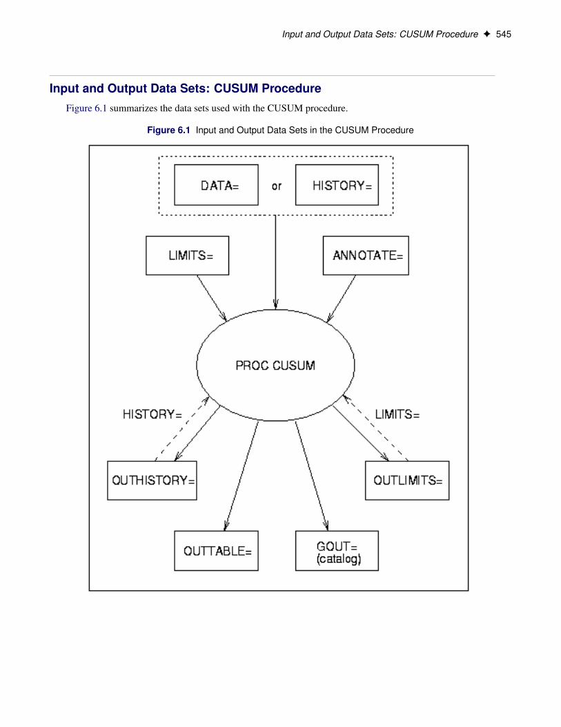
Input and Output Data Sets: CUSUM ProcedureFigure 6.1 summarizes the data sets used with the CUSUM procedure.
Figure 6.1 Input and Output Data Sets in the CUSUM Procedure

546 F Chapter 6: The CUSUM Procedure
XCHART Statement: CUSUM Procedure
Overview: XCHART StatementThe XCHART statement creates cumulative sum control charts from subgroup means or individual mea-surements. You can create these charts for one-sided cusum (decision interval) schemes or for two-sided(V-mask) schemes. A one-sided scheme is designed to detect either a positive or a negative shift from thetarget mean, and a two-sided scheme is designed to detect positive and negative shifts from the target mean.
You can use options in the XCHART statement to
• specify parameters for a decision interval or V-mask
• specify the shift ı to be detected
• specify the target mean �0
• specify a known (standard) value �0 for the process standard deviation or estimate the standarddeviation from the data using various methods
• tabulate the information displayed on the chart
• save the information displayed on the chart in an output data set
• read parameters for the cusum scheme from a data set
• display a secondary chart that plots a time trend that has been removed from the data
• add block legends and special symbol markers to reveal stratification in process data
• superimpose stars at each point to represent related multivariate factors
• display vertical and horizontal reference lines
• modify the axis values and labels
• modify the chart layout and appearance
You have three alternatives for producing cumulative sum control charts with the XCHART statement:
• ODS Graphics output is produced if ODS Graphics is enabled, for example by specifying the ODSGRAPHICS ON statement prior to the PROC statement.
• Otherwise, traditional graphics are produced by default if SAS/GRAPH® is licensed.
• Legacy line printer charts are produced when you specify the LINEPRINTER option in the PROCstatement.
See Chapter 3, “SAS/QC Graphics,” for more information about producing these different kinds of graphs.

Getting Started: XCHART Statement F 547
Getting Started: XCHART StatementThis section introduces the XCHART statement with simple examples that illustrate the most commonlyused options. Complete syntax for the XCHART statement is presented in the section “Syntax: XCHARTStatement” on page 561, and advanced examples are given in the section “Examples: XCHART Statement”on page 594.
Creating a V-Mask Cusum Chart from Raw Data
NOTE: See Two-sided Cusum Chart with V-Mask in the SAS/QC Sample Library.
A machine fills eight-ounce cans of two-cycle engine oil additive. The filling process is believed to be instatistical control, and the process is set so that the average weight of a filled can is �0 D 8:100 ounces.Previous analysis shows that the standard deviation of fill weights is �0 D 0:050 ounces. A two-sided cusumchart is used to detect shifts of at least one standard deviation in either the positive or negative direction fromthe target mean of 8.100 ounces.
Subgroup samples of four cans are selected every hour for twelve hours. The cans are weighed, and theirweights are saved in a SAS data set named Oil.
data Oil;label Hour = 'Hour';input Hour @;do i=1 to 4;
input Weight @;output;
end;drop i;datalines;
1 8.024 8.135 8.151 8.0652 7.971 8.165 8.077 8.1573 8.125 8.031 8.198 8.0504 8.123 8.107 8.154 8.0955 8.068 8.093 8.116 8.1286 8.177 8.011 8.102 8.0307 8.129 8.060 8.125 8.1448 8.072 8.010 8.097 8.1539 8.066 8.067 8.055 8.059
10 8.089 8.064 8.170 8.08611 8.058 8.098 8.114 8.15612 8.147 8.116 8.116 8.018;
The data set Oil is partially listed in Figure 6.2.

548 F Chapter 6: The CUSUM Procedure
Figure 6.2 Partial Listing of the Data Set Oil
Hour Weight
1 8.024
1 8.135
1 8.151
1 8.065
2 7.971
2 8.165
2 8.077
2 8.157
3 8.125
3 8.031
3 8.198
3 8.050
4 8.123
4 8.107
Each observation contains one value of Weight along with its associated value of Hour, and the values ofHour are in increasing order. The CUSUM procedure assumes that DATA= input data sets are sorted in this“strung-out” form.
The following statements request a two-sided cusum chart with a V-mask for the average weights:
ods graphics off;title 'Cusum Chart for Average Weights of Cans';proc cusum data=Oil;
xchart Weight*Hour /mu0 = 8.100 /* Target mean for process */sigma0 = 0.050 /* Known standard deviation */delta = 1 /* Shift to be detected */alpha = 0.10 /* Type I error probability */vaxis = -5 to 3 ;
label Weight = 'Cumulative Sum';run;
The CUSUM procedure is invoked with the PROC CUSUM statement. The DATA= option in the PROCCUSUM statement specifies that the SAS data set Oil is to be read. The variables to be analyzed are specifiedin the XCHART statement. The process measurement variable (Weight) is specified before the asterisk(this variable is referred to more generally as a process). The time variable (Hour) is specified after theasterisk (this variable is referred to more generally as a subgroup-variable because it determines how themeasurements are classified into rational subgroups).
The option ALPHA=0.10 specifies the probability of a Type 1 error for the cusum scheme (the probability ofdetecting a shift when none occurs).
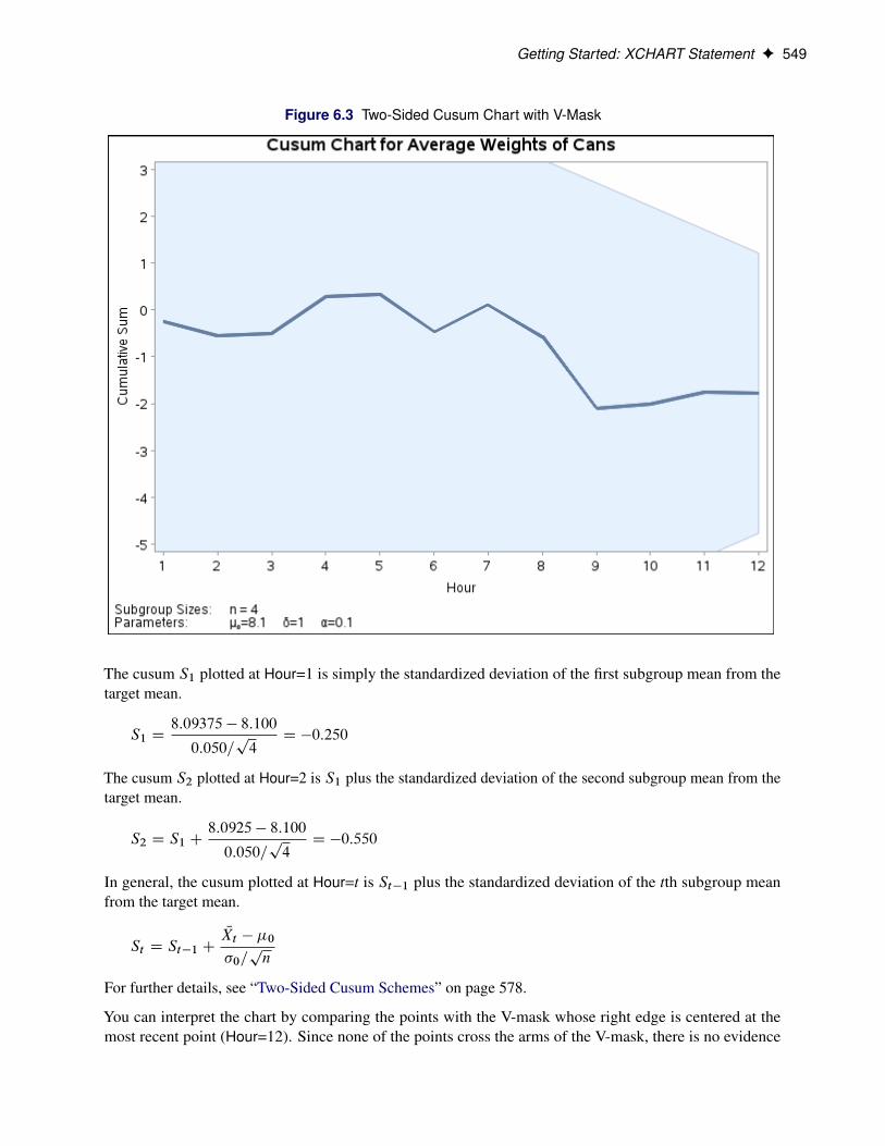
The cusum chart is shown in Figure 6.3.
Getting Started: XCHART Statement F 549
Figure 6.3 Two-Sided Cusum Chart with V-Mask
The cusum S1 plotted at Hour=1 is simply the standardized deviation of the first subgroup mean from thetarget mean.
S1 D8:09375 � 8:100
0:050=p4
D �0:250
The cusum S2 plotted at Hour=2 is S1 plus the standardized deviation of the second subgroup mean from thetarget mean.
S2 D S1 C8:0925 � 8:100
0:050=p4D �0:550
In general, the cusum plotted at Hour=t is St�1 plus the standardized deviation of the tth subgroup meanfrom the target mean.
St D St�1 CNXt � �0
�0=pn
For further details, see “Two-Sided Cusum Schemes” on page 578.
You can interpret the chart by comparing the points with the V-mask whose right edge is centered at themost recent point (Hour=12). Since none of the points cross the arms of the V-mask, there is no evidence

550 F Chapter 6: The CUSUM Procedure
that a shift has occurred, and the fluctuations in the cusums can be attributed to chance variation. In general,crossing the lower arm is evidence of an increase in the process mean, whereas crossing the upper arm isevidence of a decrease in the mean.
Creating a V-Mask Cusum Chart from Subgroup Summary Data
NOTE: See Two-sided Cusum Chart with V-Mask in the SAS/QC Sample Library.
The previous example illustrates how you can create a cusum chart using raw process measurements readfrom a DATA= data set. In many applications, however, the data are provided in summarized form as subgroupmeans. This example illustrates the use of the XCHART statement when the input data set is a HISTORY=data set.
The following data set provides the subgroup means, standard deviations, and sample sizes corresponding tothe variable Weight in the data set Oil (see the section “Creating a V-Mask Cusum Chart from Raw Data” onpage 547:
data Oilstat;label Hour = 'Hour';input Hour WeightX WeightS WeightN;datalines;
1 8.0938 0.0596 42 8.0925 0.0902 43 8.1010 0.0763 44 8.1198 0.0256 45 8.1013 0.0265 46 8.0800 0.0756 47 8.1145 0.0372 48 8.0830 0.0593 49 8.0618 0.0057 4
10 8.1023 0.0465 411 8.1065 0.0405 412 8.0993 0.0561 4;
The data set Oilstat is listed in Figure 6.4.
Figure 6.4 Listing of the Data Set Oilstat
Obs Hour WeightX WeightS WeightN
1 1 8.0938 0.0596 4
2 2 8.0925 0.0902 4
3 3 8.1010 0.0763 4
4 4 8.1198 0.0256 4
5 5 8.1013 0.0265 4
6 6 8.0800 0.0756 4
7 7 8.1145 0.0372 4
8 8 8.0830 0.0593 4
9 9 8.0618 0.0057 4
10 10 8.1023 0.0465 4
11 11 8.1065 0.0405 4
12 12 8.0993 0.0561 4
Getting Started: XCHART Statement F 551
Since the data set contains a subgroup variable, a mean variable, a standard deviation variable, and a samplesize variable, it can be read as a HISTORY= data set. Note that the names WeightX, WeightS, and WeightNsatisfy the naming conventions for summary variables since they begin with a common prefix (Weight) andend with the suffix letters X, S, and N.
The following statements create the cusum chart:
title 'Cusum Chart for Average Weights of Cans';proc cusum history=Oilstat;
xchart Weight*Hour /mu0 = 8.100 /* target mean */sigma0 = 0.050 /* known standard deviation */delta = 1 /* shift to be detected */alpha = 0.10 /* Type 1 error probability */vaxis = -5 to 3 ;
label WeightX = 'Cumulative Sum';run;
Note that the process Weight specified in the XCHART statement is the prefix of the summary variable namesin Oilstat. Also note that the vertical axis label is specified by associating a variable label with the subgroupmean variable (WeightX). The chart (not shown here) is identical to the one in Figure 6.2.
In general, a HISTORY= input data set used with the XRCHART statement must contain the following fourvariables:
• subgroup variable
• subgroup mean variable
• subgroup range variable
• subgroup sample size variable
Furthermore, the names of subgroup mean, standard deviation, and sample size variables must begin with theprefix process specified in the XRCHART statement and end with the special suffix characters X, S, and N,respectively.
Note that the interpretation of process depends on the input data set specified in the PROC CUSUM statement.
• If raw data are read using the DATA= option (as in the previous example), process is the name of theSAS variable containing the process measurements.
• If summary data are read using the HISTORY= option (as in this example), process is the commonprefix for the names containing the summary statistics.
For more information, see “DATA= Data Set” on page 592 and “HISTORY= Data Set” on page 593.

552 F Chapter 6: The CUSUM Procedure
Saving Summary Statistics
NOTE: See Two-sided Cusum Chart with V-Mask in the SAS/QC Sample Library.
In this example, the CUSUM procedure is used to save summary statistics and cusums in an output dataset. The summary statistics can subsequently be analyzed by the CUSUM procedure (as in the precedingexample). The following statements read the raw measurements from the data set Oil (see “Creating a V-MaskCusum Chart from Raw Data” on page 547) and create a summary data set named Oilhist:
title 'Cusum Chart for Average Weights of Cans';proc cusum data=Oil;
xchart Weight*Hour /nochartouthistory = Oilhistmu0 = 8.100 /* Target mean for process */sigma0 = 0.050 /* Known standard deviation */delta = 1 /* Shift to be detected */alpha = 0.10 /* Type I error probability */vaxis = -5 to 3 ;
label Weight = 'Cumulative Sum';run;
The OUTHISTORY= option names the SAS data set containing the summary information, and the NOCHARToption suppresses the display of the charts (since the purpose here is simply to create an output data set).Figure 6.5 lists the data set Oilhist.
Figure 6.5 Listing of the Data Set Oilhist
Cusum Chart for Average Weights of CansCusum Chart for Average Weights of Cans
Obs Hour WeightX WeightS WeightC WeightN
1 1 8.0938 0.0596 -.2500 4
2 2 8.0925 0.0902 -.5500 4
3 3 8.1010 0.0763 -.5100 4
4 4 8.1198 0.0256 0.2800 4
5 5 8.1013 0.0265 0.3300 4
6 6 8.0800 0.0756 -.4700 4
7 7 8.1145 0.0372 0.1100 4
8 8 8.0830 0.0593 -.5700 4
9 9 8.0618 0.0057 -2.100 4
10 10 8.1023 0.0465 -2.010 4
11 11 8.1065 0.0405 -1.750 4
12 12 8.0993 0.0561 -1.780 4
There are five variables in the data set.
• Hour contains the subgroup index
• WeightX contains the subgroup means
• WeightS contains the subgroup standard deviations
• WeightC contains the cumulative sums

Getting Started: XCHART Statement F 553
• WeightN contains the subgroup sample sizes
Note that the variables in the OUTHISTORY= data set are named by adding the suffix characters X, S, N, andC to the process Weight specified in the XCHART statement. In other words, the variable naming conventionfor OUTHISTORY= data sets is the same as for HISTORY= data sets.
For more information, see “OUTHISTORY= Data Set” on page 589.
Creating a One-Sided Cusum Chart with a Decision Interval
NOTE: See One-sided Cusum Chart in the SAS/QC Sample Library.
An alternative to the V-mask cusum chart is the one-sided cusum chart with a decision interval, which issometimes referred to as the “computational form of the cusum chart.” This example illustrates how you cancreate a one-sided cusum chart for individual measurements.
A can of oil is selected every hour for fifteen hours. The cans are weighed, and their weights are saved in aSAS data set named Cans:1
data Cans;length comment $16;label Hour = 'Hour';input Hour Weight comment $16. ;datalines;
1 8.0242 7.9713 8.1254 8.1235 8.0686 8.177 Pump Adjusted7 8.229 Pump Adjusted8 8.0729 8.066
10 8.08911 8.05812 8.14713 8.14114 8.04715 8.125;
Suppose the problem is to detect a positive shift in the process mean of one standard deviation (ı D 1) fromthe target of 8.100 ounces. Furthermore, suppose that
• a known value �0 D 0:050 is available for the process standard deviation
• an in-control average run length (ARL) of approximately 100 is required
• an ARL of approximately five is appropriate for detecting the shift
1This data set is used by later examples in this chapter.

554 F Chapter 6: The CUSUM Procedure
Table 6.4 indicates that these ARLs can be achieved with the decision interval h = 3 and the reference value k= 0.5. The following statements use these parameters to create the chart and tabulate the cusum scheme:
options nogstyle;goptions ftext=swiss;symbol v=dot color=salmon h=1.8 pct;title "One-Sided Cusum Analysis";proc cusum data=Cans;
xchart Weight*Hour /mu0 = 8.100 /* target mean for process */sigma0 = 0.050 /* known standard deviation */delta = 1 /* shift to be detected */h = 3 /* cusum parameter h */k = 0.5 /* cusum parameter k */scheme = onesided /* one-sided decision interval */tableall /* table */cinfill = ywhcframe = bigbcout = salmoncconnect = salmonclimits = blackcoutfill = bilg;
label Weight = 'Cusum of Weight';run;options gstyle;
The NOGSTYLE system option causes ODS styles not to affect traditional graphics. Instead, the SYMBOLstatement, GOPTIONS, and XCHART statement options control the appearance of the graph. The GSTYLEsystem option restores the use of ODS styles for traditional graphics produced subsequently. The chart isshown in Figure 6.6.
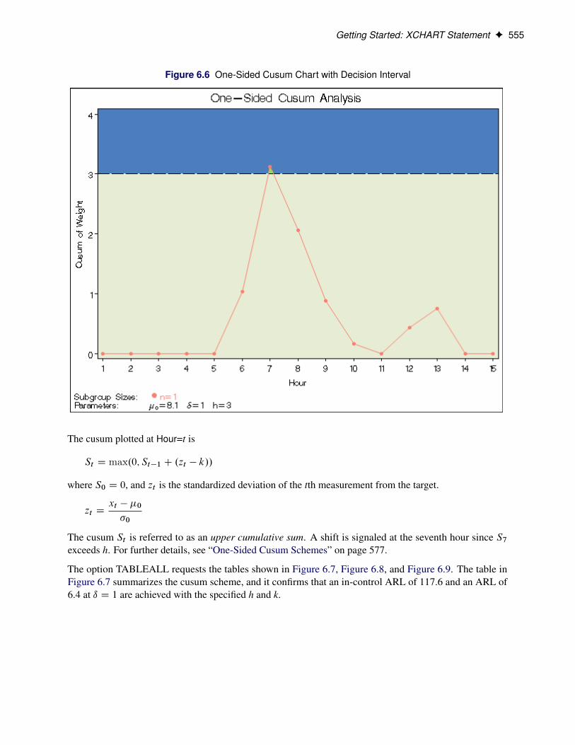
Getting Started: XCHART Statement F 555
Figure 6.6 One-Sided Cusum Chart with Decision Interval
The cusum plotted at Hour=t is
St D max.0; St�1 C .zt � k//
where S0 D 0, and zt is the standardized deviation of the tth measurement from the target.
zt Dxt � �0
�0
The cusum St is referred to as an upper cumulative sum. A shift is signaled at the seventh hour since S7exceeds h. For further details, see “One-Sided Cusum Schemes” on page 577.
The option TABLEALL requests the tables shown in Figure 6.7, Figure 6.8, and Figure 6.9. The table inFigure 6.7 summarizes the cusum scheme, and it confirms that an in-control ARL of 117.6 and an ARL of6.4 at ı D 1 are achieved with the specified h and k.

556 F Chapter 6: The CUSUM Procedure
Figure 6.7 Summary Table
Cusum Parameters
Process Variable Weight (Cusum of Weight)
Subgroup Variable Hour (Hour)
Scheme One-Sided
Target Mean (Mu0) 8.1
Sigma0 0.05
Delta 1
Nominal Sample Size 1
h 3
k 0.5
Average Run Length (Delta) 6.40390895
Average Run Length (0) 117.595692
The table in Figure 6.8 tabulates the information displayed in Figure 6.6.
Figure 6.8 Tabulation of One-Sided Chart
One-Sided Cusum Analysis
The CUSUM Procedure
One-Sided Cusum Analysis
The CUSUM Procedure
Cumulative Sum Chart Summary for Weight
Hour
SubgroupSample
SizeIndividual
Value CusumDecision
Interval
DecisionInterval
Exceeded
1 1 8.0240000 0.0000000 3.0000
2 1 7.9710000 0.0000000 3.0000
3 1 8.1250000 0.0000000 3.0000
4 1 8.1230000 0.0000000 3.0000
5 1 8.0680000 0.0000000 3.0000
6 1 8.1770000 1.0400000 3.0000
7 1 8.2290000 3.1200000 3.0000 Upper
8 1 8.0720000 2.0600000 3.0000
9 1 8.0660000 0.8800000 3.0000
10 1 8.0890000 0.1600000 3.0000
11 1 8.0580000 0.0000000 3.0000
12 1 8.1470000 0.4400000 3.0000
13 1 8.1410000 0.7600000 3.0000
14 1 8.0470000 0.0000000 3.0000
15 1 8.1250000 0.0000000 3.0000
The table in Figure 6.9 presents the computational form of the cusum scheme described by Lucas (1976).

Getting Started: XCHART Statement F 557
Figure 6.9 Computational Form of Cusum Scheme
One-Sided Cusum Analysis
The CUSUM Procedure
One-Sided Cusum Analysis
The CUSUM Procedure
Computational Cumulative Sum for Weight
Hour
SubgroupSample
SizeIndividual
ValueUpper
Cusum
Number ofConsecutive
Upper Sums > 0
1 1 8.0240000 0.0000000 0
2 1 7.9710000 0.0000000 0
3 1 8.1250000 0.0000000 0
4 1 8.1230000 0.0000000 0
5 1 8.0680000 0.0000000 0
6 1 8.1770000 1.0400000 1
7 1 8.2290000 3.1200000 2
8 1 8.0720000 2.0600000 3
9 1 8.0660000 0.8800000 4
10 1 8.0890000 0.1600000 5
11 1 8.0580000 0.0000000 0
12 1 8.1470000 0.4400000 1
13 1 8.1410000 0.7600000 2
14 1 8.0470000 0.0000000 0
15 1 8.1250000 0.0000000 0
Following the method of Lucas (1976), the process average at the out-of-control point (Hour=7) can beestimated as
�0 C �0.N7k C S7/=.N7pn/
D 8:10C 0:05.2.0:5/C 3:12/=2
D 8:203 ounces
where S7 D 3:12 is the upper sum at Hour=7, and N7 D 2 is the number of successive positive upper sumsat Hour=7.
Saving Cusum Scheme Parameters
NOTE: See One-sided Cusum Chart in the SAS/QC Sample Library.
This example is a continuation of the previous example that illustrates how to save cusum scheme parametersin a data set specified with the OUTLIMITS= option. This enables you to apply the parameters to future dataor to subsequently modify the parameters with a DATA step program.

558 F Chapter 6: The CUSUM Procedure
ods graphics on;title 'One-Sided Cusum Analysis';proc cusum data=Cans;
xchart Weight*Hour /mu0 = 8.100 /* target mean for process */sigma0 = 0.050 /* known standard deviation */delta = 1 /* shift to be detected */h = 3 /* cusum parameter h */k = 0.5 /* cusum parameter k */scheme = onesided /* one-sided decision interval */outlimits = cusparmodstitle = titlemarkers;
label Weight = 'Cusum of Weight';run;
The chart, shown in Figure 6.10, is similar to the one in Figure 6.6 but is created by using ODS Graphicsbecause the ODS GRAPHICS ON statement is specified before the PROC CUSUM statement.
Figure 6.10 One-Sided Cusum Scheme with Decision Interval
The OUTLIMITS= data set is listed in Figure 6.11.

Getting Started: XCHART Statement F 559
Figure 6.11 Listing of the OUTLIMITS= Data Set cusparm
One-Sided Cusum AnalysisOne-Sided Cusum Analysis
Obs _VAR_ _SUBGRP_ _TYPE_ _LIMITN_ _H_ _K_ _SCHEME_ _MU0_ _DELTA_
1 Weight Hour STANDARD 1 3 0.5 ONESIDED 8.1 1
Obs _MEAN_ _STDDEV_ _ARLIN_ _ARLOUT_
1 8.09747 0.05 117.596 6.40391
The data set contains one observation with the parameters for process Weight. The variables _TYPE_, _H_,_K_, _MU0_, _DELTA_, and _STDDEV_ save the parameters specified with the options SCHEME=, H=, K=,MU0=, DELTA=, and SIGMA0=, respectively. The variable _MEAN_ saves an estimate of the process mean,and the variable _LIMITN_ saves the nominal sample size. The variables _ARLIN_ and _ARLOUT_ save theaverage run lengths for ı D 0 and for ı D 1.
The variables _VAR_ and _SUBGRP_ save the process and subgroup-variable. The variable _TYPE_ is abookkeeping variable that indicates whether the value of _STDDEV_ is an estimate or a standard value.
For more information, see “OUTLIMITS= Data Set” on page 588.
Reading Cusum Scheme Parameters
NOTE: See One-sided Cusum Chart in the SAS/QC Sample Library.
This example shows how the cusum parameters saved in the previous example can be applied to newmeasurements saved in a data set named Cans2:
data Cans2;length pump $ 8;label Hour = 'Hour';input Hour Weight pump $ 8. ;datalines;
16 8.1765 Pump 317 8.0949 Pump 318 8.1393 Pump 319 8.1491 Pump 320 8.0473 Pump 121 8.1602 Pump 122 8.0633 Pump 123 8.0921 Pump 124 8.1573 Pump 125 8.1304 Pump 126 8.0979 Pump 127 8.2407 Pump 128 8.0730 Pump 129 8.0986 Pump 230 8.0785 Pump 231 8.2308 Pump 232 8.0986 Pump 233 8.0782 Pump 234 8.1435 Pump 235 8.0666 Pump 2;
560 F Chapter 6: The CUSUM Procedure
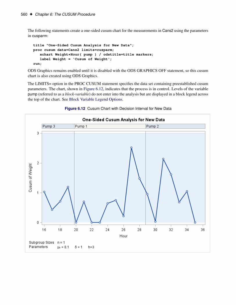
The following statements create a one-sided cusum chart for the measurements in Cans2 using the parametersin cusparm:
title "One-Sided Cusum Analysis for New Data";proc cusum data=Cans2 limits=cusparm;
xchart Weight*Hour( pump ) / odstitle=title markers;label Weight = 'Cusum of Weight';
run;
ODS Graphics remains enabled until it is disabled with the ODS GRAPHICS OFF statement, so this cusumchart is also created using ODS Graphics.
The LIMITS= option in the PROC CUSUM statement specifies the data set containing preestablished cusumparameters. The chart, shown in Figure 6.12, indicates that the process is in control. Levels of the variablepump (referred to as a block-variable) do not enter into the analysis but are displayed in a block legend acrossthe top of the chart. See Block Variable Legend Options.
Figure 6.12 Cusum Chart with Decision Interval for New Data

Syntax: XCHART Statement F 561
In general, the parameters for a specified process and subgroup-variable are read from the first observation inthe LIMITS= data set for which
• the value of _VAR_ matches the process (in this case, Weight)
• the value of _SUBGRP_ matches the subgroup-variable name (in this case, Hour)
If you are maintaining more than one set of cusum parameters for a particular process, you will find itconvenient to include a special identifier variable named _INDEX_ in the LIMITS= data set. This must be acharacter variable of length 16. Then, if you specify READINDEX=’value’ in the XCHART statement, theparameters for a specified process and subgroup-variable are read from the first observation in the LIMITS=data set for which
• the value of _VAR_ matches process
• the value of _SUBGRP_ matches the subgroup-variable name
• the value of _INDEX_ matches value
In this example, the LIMITS= data set was created in a previous run of the CUSUM procedure. You can alsocreate a LIMITS= data set with the DATA step. See “LIMITS= Data Set” on page 592 for details concerningthe variables that you must provide.
Syntax: XCHART StatementThe basic syntax for a one-sided (decision interval) scheme using the XCHART statement is as follows:
XCHART process � subgroup-variable / SCHEME=ONESIDED MU0=target DELTA=shift H=h< options > ;
The general form of this syntax is as follows:
XCHART processes � subgroup-variable < (block-variables) >< =symbol-variable =’character ’ > / SCHEME=ONESIDED MU0=target DELTA=shift H=h< options > ;
Note that the options SCHEME=ONESIDED, MU0=, DELTA=, and H= are required unless their values areread from a LIMITS= data set.
The basic syntax for a two-sided (V-mask) scheme is as follows:
XCHART process � subgroup-variable / MU0=target DELTA=shift ALPHA=alpha H=h < options > ;
The general form of this syntax is as follows:
XCHART processes � subgroup-variable < (block-variables) >< =symbol-variable | = ’character ’ > / MU0=target DELTA=shift ALPHA=alpha H=h< options > ;
Note that the options MU0=, DELTA=, and either ALPHA= or H= are required unless their values are readfrom a LIMITS= data set.
You can use any number of XCHART statements in the CUSUM procedure. The components of the XCHARTstatement are described as follows.

562 F Chapter 6: The CUSUM Procedure
process
processesidentify one or more processes to be analyzed. The specification of process depends on the input dataset specified in the PROC CUSUM statement.
• If raw data are read from a DATA= data set, process must be the name of the variable containingthe raw measurements. For an example, see “Creating a V-Mask Cusum Chart from Raw Data”on page 547.
• If summary data are read from a HISTORY= data set, process must be the common prefix of thesummary variables in the HISTORY= data set. For an example, see “Creating a V-Mask CusumChart from Subgroup Summary Data” on page 550.
A process is required. If more than one process is specified, enclose the list in parentheses. Theparameters specified in the XCHART statement are applied to all of the processes.2
subgroup-variableis the variable that classifies the data into subgroups. The subgroup-variable is required. In theexamples “Creating a V-Mask Cusum Chart from Raw Data” on page 547 and “Creating a V-MaskCusum Chart from Subgroup Summary Data” on page 550, Hour is the subgroup variable.
block-variablesare optionally specified variables that group the data into blocks of consecutive subgroups. Theblocks are labeled in a legend, and each block-variable provides one level of labels in the legend. SeeFigure 6.12 for an example.
symbol-variableis an optionally specified variable whose levels (unique values) determine the plotting character orsymbol marker used to plot the cusums.
• If you produce a line printer chart, an ‘A’ marks points corresponding to the first level of thesymbol-variable, a ‘B’ marks points corresponding to the second level, and so on.
• If you produce traditional graphics, distinct symbol markers are displayed for points correspond-ing to the various levels of the symbol-variable. You can specify the symbol markers withSYMBOLn statements.
characterspecifies a plotting character for line printer charts. See Figure 6.10 for an example.
optionsspecify optional cusum parameters, enhance the appearance of the chart, request additional analyses,save results in data sets, and so on. The section “Summary of Options”, which follows, lists all optionsby function.
2For this reason, it may be preferable to read distinct cusum parameters for each process from a LIMITS= data set.

Syntax: XCHART Statement F 563
Summary of Options
The following tables list the XCHART statement options by function. Options unique to the CUSUMprocedure are listed in Table 6.1, and are described in detail in the section “Dictionary of Special Options” onpage 570. Options that are common to both the CUSUM and SHEWHART procedures are listed in Table 6.2.They are described in detail in “Dictionary of Options: SHEWHART Procedure” on page 1946.
Table 6.1 XCHART Statement Special Options
Option Description
Options for Specifying a One-Sided (Decision Interval) Cusum SchemeDELTA= specifies shift to be detected as a multiple of standard errorH= specifies decision interval h (h > 0) as a multiple of standard
errorHEADSTART= specifies headstart value S0 as a multiple of standard errorK= specifies reference value k (k > 0)LIMITN= specifies fixed nominal sample size for cusum schemeLIMITN= specifies that cusums are to be computed for all subgroups
regardless of sample sizeMU0= specifies target �0 for meanNOREADLIMITS specifies that cusum parameters are not to be read from LIM-
ITS= data set (SAS 6.10 and later releases)READINDEX= reads cusum scheme parameters from a LIMITS= data setREADLIMITS specifies that cusum parameters are to be read from LIMITS=
data set (SAS 6.09 and earlier releases)SCHEME=ONESIDED specifies a one-sided schemeSHIFT= specifies shift to be detected in data unitsSIGMA0= specifies standard (known) value �0 for process standard devia-
tionOptions for Specifying a Two-Sided (V-Mask) Cusum SchemeALPHA= specifies probability of Type 1 errorBETA= specifies probability of Type 2 errorH= specifies vertical distance between V-mask origin and upper (or
lower) armK= specifies slope of lower arm of V-maskLIMITN= specifies fixed nominal sample size for cusum schemeLIMITN= specifies that cusums are to be computed for all subgroups
regardless of sample sizeNOREADLIMITS specifies that cusum parameters are not to be read from LIM-
ITS= data set (SAS 6.10 and later releases)READINDEX= reads cusum scheme parameters from a LIMITS= data setREADLIMITS specifies that cusum parameters are to be read from LIMITS=
data set (SAS 6.09 and earlier releases)READSIGMAS reads _SIGMAS_ instead of _ALPHA_ from LIMITS= data set
when both variables are availableSIGMAS= specifies probability of Type 1 error as probability that standard
normally distributed variable exceeds value in absolute value

564 F Chapter 6: The CUSUM Procedure
Table 6.1 continued
Option Description
Options for Estimating Process Standard DeviationSMETHOD= specifies method for estimating process standard deviation �TYPE= identifies whether _STDDEV_ in OUTLIMITS= data set is
an estimate or standard, and specifies value of _TYPE_ inOUTLIMITS= data set
Options for Displaying Decision Interval or V-MaskCINFILL= specifies color for area under decision interval line or inside
V-maskCLIMITS= specifies color of decision interval lineCMASK= specifies color of V-mask outlineLLIMITS= specifies line type for decision intervalLMASK= specifies line type for V-mask armsNOMASK suppresses display of V-maskORIGIN= specifies value of subgroup-variable locating origin of V-maskWLIMITS= specifies line width for decision intervalWMASK= specifies line width for V-maskTabulation OptionsTABLEALL specifies the options TABLECHART, TABLECOMP,
TABLEID, TABLEOUT, and TABLESUMMARYTABLECHART tabulates the information displayed in the cusum chartTABLECOMP tabulates the computational form of the cusum scheme as de-
scribed by Lucas (1976) and Lucas and Crosier (1982)TABLEID augments TABLECHART and TABLECOMP tables with
columns for ID variablesTABLEOUT augments TABLECHART table with a column indicating if the
decision interval or V-mask was exceededTABLESUMMARY tabulates the parameters for the cusum scheme and the average
run lengths corresponding to shifts of zero and ı
Table 6.2 XCHART Statement General Options
Option Description
Options for Plotting and Labeling PointsALLLABEL= labels every point on cusum chartALLLABEL2= labels every point on trend chartCLABEL= specifies color for labelsCCONNECT= specifies color for line segments that connect points on
chartCFRAMELAB= specifies fill color for frame around labeled pointsCOUT= specifies color for portions of line segments that connect
points outside control limitsCOUTFILL= specifies color for shading areas between the connected
points and control limits outside the limitsLABELANGLE= specifies angle at which labels are drawn

Syntax: XCHART Statement F 565
Table 6.2 continued
Option Description
LABELFONT= specifies software font for labelsLABELHEIGHT= specifies height of labelsNOCONNECT suppresses line segments that connect points on chartNOTRENDCONNECT suppresses line segments that connect points on trend
chartOUTLABEL= labels points outside control limitsSYMBOLLEGEND= specifies LEGEND statement for levels of symbol-
variableSYMBOLORDER= specifies order in which symbols are assigned for levels
of symbol-variableTURNALL|TURNOUT turns point labels so that they are strung out verticallyAxis and Axis Label OptionsCAXIS= specifies color for axis lines and tick marksCFRAME= specifies fill colors for frame for plot areaCTEXT= specifies color for tick mark values and axis labelsDISCRETE produces horizontal axis for discrete numeric group val-
uesHAXIS= specifies major tick mark values for horizontal axisHEIGHT= specifies height of axis label and axis legend textHMINOR= specifies number of minor tick marks between major tick
marks on horizontal axisHOFFSET= specifies length of offset at both ends of horizontal axisINTSTART= specifies first major tick mark value on horizontal axis
when a date, time, or datetime format is associated withnumeric subgroup variable
NOHLABEL suppresses label for horizontal axisNOTICKREP specifies that only the first occurrence of repeated, adja-
cent subgroup values is to be labeled on horizontal axisNOVANGLE requests vertical axis labels that are strung out verticallySKIPHLABELS= specifies thinning factor for tick mark labels on horizontal
axisSPLIT= specifies splitting character for axis labelsTURNHLABELS requests horizontal axis labels that are strung out verti-
callyVAXIS= specifies major tick mark values for vertical axis of cusum
chartVAXIS2= specifies major tick mark values for vertical axis of trend
chartVFORMAT= specifies format for primary vertical axis tick mark labelsVFORMAT2= specifies format for secondary vertical axis tick mark
labelsVMINOR= specifies number of minor tick marks between major tick
marks on vertical axisVOFFSET= specifies length of offset at both ends of vertical axis

566 F Chapter 6: The CUSUM Procedure
Table 6.2 continued
Option Description
WAXIS= specifies width of axis linesPlot Layout OptionsALLN plots means for all subgroupsBILEVEL creates control charts using half-screens and half-pagesEXCHART creates control charts for a process only when exceptions
occurINTERVAL= natural time interval between consecutive subgroup po-
sitions when time, date, or datetime format is associatedwith a numeric subgroup variable
MAXPANELS= maximum number of pages or screens for chartNMARKERS requests special markers for points corresponding to sam-
ple sizes not equal to nominal sample size for fixed con-trol limits
NOCHART suppresses creation of chartNOFRAME suppresses frame for plot areaNOLEGEND suppresses legend for subgroup sample sizesNPANELPOS= specifies number of subgroup positions per panel on each
chartREPEAT repeats last subgroup position on panel as first subgroup
position of next panelTOTPANELS= specifies number of pages or screens to be used to display
chartTRENDVAR= specifies list of trend variablesYPCT1= specifies length of vertical axis on cusum chart as a per-
centage of sum of lengths of vertical axes for cusum andtrend charts
Reference Line OptionsCHREF= specifies color for lines requested by HREF= and
HREF2= optionsCVREF= specifies color for lines requested by VREF= and
VREF2= optionsHREF= specifies position of reference lines perpendicular to hori-
zontal axis on cusum chartHREF2= specifies position of reference lines perpendicular to hori-
zontal axis on trend chartHREFDATA= specifies position of reference lines perpendicular to hori-
zontal axis on cusum chartHREF2DATA= specifies position of reference lines perpendicular to hori-
zontal axis on trend chartHREFLABELS= specifies labels for HREF= linesHREF2LABELS= specifies labels for HREF2= linesHREFLABPOS= specifies position of HREFLABELS= and
HREF2LABELS= labelsLHREF= specifies line type for HREF= and HREF2= lines

Syntax: XCHART Statement F 567
Table 6.2 continued
Option Description
LVREF= specifies line type for VREF= and VREF2= linesNOBYREF specifies that reference line information in a data set
applies uniformly to charts created for all BY groupsVREF= specifies position of reference lines perpendicular to ver-
tical axis on cusum chartVREF2= specifies position of reference lines perpendicular to ver-
tical axis on trend chartVREFLABELS= specifies labels for VREF= linesVREF2LABELS= specifies labels for VREF2= linesVREFLABPOS= position of VREFLABELS= and VREF2LABELS= la-
belsGrid OptionsCGRID= specifies color for grid requested with GRID or END-
GRID optionENDGRID adds grid after last plotted pointGRID adds grid to control chartLENDGRID= specifies line type for grid requested with the ENDGRID
optionLGRID= specifies line type for grid requested with the GRID op-
tionWGRID= specifies width of grid linesGraphical Enhancement OptionsANNOTATE= specifies annotate data set that adds features to cusum
chartANNOTATE2= specifies annotate data set that adds features to trend chartDESCRIPTION= specifies description of cusum chart’s GRSEG catalog
entryFONT= specifies software font for labels and legends on chartsNAME= specifies name of cusum chart’s GRSEG catalog entryPAGENUM= specifies the form of the label used in paginationPAGENUMPOS= specifies the position of the page number requested with
the PAGENUM= optionWTREND= specifies width of line segments connecting points on
trend chart
Options for Producing Graphs Using ODS StylesBLOCKVAR= specifies one or more variables whose values define colors
for filling background of block-variable legendCFRAMELAB draws a frame around labeled pointsCOUT draw portions of line segments that connect points outside
control limits in a contrasting colorCSTAROUT specifies that portions of stars exceeding inner or outer
circles are drawn using a different color

568 F Chapter 6: The CUSUM Procedure
Table 6.2 continued
Option Description
OUTFILL shades areas between control limits and connected pointslying outside the limits
STARFILL= specifies a variable identfying groups of stars filled withdifferent colors
STARS= specifies a variable identfying groups of stars whose out-lines are drawn with different colors
Options for ODS GraphicsBLOCKREFTRANSPARENCY= specifies the wall fill transparency for blocks and phasesINFILLTRANSPARENCY= specifies the control limit infill transparencyMARKERS plots subgroup points with markersNOBLOCKREF suppresses block and phase reference linesNOBLOCKREFFILL suppresses block and phase wall fillsNOFILLLEGEND suppresses legend for levels of a STARFILL= variableNOPHASEREF suppresses block and phase reference linesNOPHASEREFFILL suppresses block and phase wall fillsNOREF suppresses block and phase reference linesNOREFFILL suppresses block and phase wall fillsNOSTARFILLLEGEND suppresses legend for levels of a STARFILL= variableNOTRANSPARENCY disables transparency in ODS Graphics outputODSFOOTNOTE= specifies a graph footnoteODSFOOTNOTE2= specifies a secondary graph footnoteODSLEGENDEXPAND specifies that legend entries contain all levels observed in
the dataODSTITLE= specifies a graph titleODSTITLE2= specifies a secondary graph titleOUTFILLTRANSPARENCY= specifies control limit outfill transparencyOVERLAYURL= specifies URLs to associate with overlay pointsOVERLAY2URL= specifies URLs to associate with overlay points on sec-
ondary chartPHASEPOS= specifies vertical position of phase legendPHASEREFLEVEL= associates phase and block reference lines with either
innermost or the outermost levelPHASEREFTRANSPARENCY= specifies the wall fill transparency for blocks and phasesREFFILLTRANSPARENCY= specifies the wall fill transparency for blocks and phasesSIMULATEQCFONT draws central line labels using a simulated software fontSTARTRANSPARENCY= specifies star fill transparencyURL= specifies a variable whose values are URLs to be associ-
ated with subgroupsURL2= specifies a variable whose values are URLs to be associ-
ated with subgroups on secondary chartInput Data Set OptionsMISSBREAK specifies that observations with missing values are not to
be processed

Syntax: XCHART Statement F 569
Table 6.2 continued
Option Description
Output Data Set OptionsOUTHISTORY= creates output data set containing subgroup summary
statisticsOUTINDEX= specifies value of _INDEX_ in the OUTLIMITS= data setOUTLIMITS= creates output data set containing control limitsOUTTABLE= creates output data set containing subgroup summary
statistics and control limitsSpecification Limit OptionsCIINDICES specifies ˛ value and type for computing capability index
confidence limitsLSL= specifies list of lower specification limitsTARGET= specifies list of target valuesUSL= specifies list of upper specification limits
Block Variable Legend OptionsBLOCKLABELPOS= specifies position of label for block-variable legendBLOCKLABTYPE= specifies text size of block-variable legendBLOCKPOS= specifies vertical position of block-variable legendBLOCKREP repeats identical consecutive labels in block-variable leg-
endCBLOCKLAB= specifies fill colors for frames enclosing variable labels
in block-variable legendCBLOCKVAR= specifies one or more variables whose values are colors
for filling background of block-variable legendPhase OptionsCPHASELEG= specifies text color for phase legendOUTPHASE= specifies value of _PHASE_ in the OUTHISTORY= data
setPHASEBREAK disconnects last point in a phase from first point in next
phasePHASELABTYPE= specifies text size of phase legendPHASELEGEND displays phase labels in a legend across top of chartPHASELIMITS labels control limits for each phase, provided they are
constant within that phasePHASEREF delineates phases with vertical reference linesREADPHASES= specifies phases to be read from an input data setStar OptionsCSTARCIRCLES= specifies color for STARCIRCLES= circlesCSTARFILL= specifies color for filling starsCSTAROUT= specifies outline color for stars exceeding inner or outer
circlesCSTARS= specifies color for outlines of starsLSTARCIRCLES= specifies line types for STARCIRCLES= circles

570 F Chapter 6: The CUSUM Procedure
Table 6.2 continued
Option Description
LSTARS= specifies line types for outlines of STARVERTICES=stars
STARBDRADIUS= specifies radius of outer bound circle for vertices of starsSTARCIRCLES= specifies reference circles for starsSTARINRADIUS= specifies inner radius of starsSTARLABEL= specifies vertices to be labeledSTARLEGEND= specifies style of legend for star verticesSTARLEGENDLAB= specifies label for STARLEGEND= legendSTAROUTRADIUS= specifies outer radius of starsSTARSPECS= specifies method used to standardize vertex variablesSTARSTART= specifies angle for first vertexSTARTYPE= specifies graphical style of starSTARVERTICES= superimposes star at each point on cusum chartWSTARCIRCLES= specifies width of STARCIRCLES= circlesWSTARS= specifies width of STARVERTICES= starsOptions for Interactive Control ChartsHTML= specifies a variable whose values create links to be asso-
ciated with subgroupsHTML2= specifies variable whose values create links to be associ-
ated with subgroups on secondary chartHTML_LEGEND= specifies a variable whose values create links to be asso-
ciated with symbols in the symbol legendWEBOUT= creates an OUTTABLE= data set with additional graphics
coordinate dataOptions for Line Printer ChartsCONNECTCHAR= specifies character used to form line segments that con-
nect points on chartHREFCHAR= specifies line character for HREF= and HREF2= linesSYMBOLCHARS= specifies characters indicating symbol-variableVREFCHAR= specifies line character for VREF= and VREF2= lines
Dictionary of Special Options
General OptionsYou can specify the following options when you use either ODS Graphics or traditional graphics:
ALPHA=valuespecifies the probability ˛ of incorrectly deciding that a shift has occurred when the process meanis equal to the target mean. This is known as the probability of a Type 1 error. The value must bebetween zero and one, and it is typically set at 0.05 or 0.10. If you specify the ALPHA= option, theerror probability approach is used to determine the V-mask. For details, see “Defining the V-Mask fora Two-Sided Cusum Scheme” on page 580.
The ALPHA= option is applicable only with two-sided cusum schemes. As an alternative to theALPHA= value, you can specify the percentile z1�˛=2 from a standard normal distribution with the

Syntax: XCHART Statement F 571
SIGMAS= option. As a second alternative, you can specify the geometric parameter h for the V-mask(in standard error units) with the H= option.
In addition to the ALPHA= option, you can optionally specify the probability of a Type 2 error withthe BETA= option.
BETA=valuespecifies the probability ˇ of failing to discover that the specified shift has occurred. This is known asthe probability of a Type 2 error. The value must be between zero and one. The BETA= option is usedin conjunction with either the ALPHA= option or the SIGMAS= option.
The interpretation of ˇ is based on the analogy between cusum charts and sequential probability ratiotests, and it is inexact since the cusum chart does not provide an acceptance region. Refer to Johnson(1961) and van Dobben de Bruyn (1968) for further details.
DATAUNITScomputes cumulative sums without standardizing the subgroup means or individual measurements. Asa result, the vertical axis of the cusum chart is scaled in the same units as the data.
The DATAUNITS option requires constant subgroup sample sizes. If your data do not have constantsubgroup sample sizes, you need to specify a constant nominal sample size n for the V-mask or decisioninterval with the LIMITN= option or with the variable _LIMITN_ in the LIMITS= data set.
DELTA=valuespecifies the absolute value of the smallest shift to be detected as a multiple ı of the process standarddeviation � or the standard error � NX , depending on whether ı is viewed as a shift in the populationmean or a shift in the sampling distribution of the subgroup mean NX , respectively.
If you specify SCHEME=ONESIDED (see the SCHEME= option later in this list) and the value ispositive, a shift above the process mean is to be detected, whereas if the value is negative, a shift belowthe process mean is to be detected.
As an alternative to specifying the DELTA= option, you can specify the shift in the same units as thedata with the SHIFT= option.
H=valuespecifies the decision interval h for a one-sided cusum scheme. This type of scheme is completelyspecified by the parameters h and k (see the K= option later in this list). You can also specify the H=option as an alternative to the ALPHA= or SIGMAS= options for a two-sided cusum scheme with aV-mask. In this case, the H= option specifies the vertical distance h between the origin for the V-maskand the upper or lower arm of the V-mask. In either case, the H=value must be positive and must beexpressed as a multiple of standard error.
You can use a table of average run lengths to choose h (this is typically between zero and 10). SeeTable 6.4 and Table 6.5
HEADSTART=value
HSTART=valuespecifies a headstart value S0 for a one-sided cusum scheme. The value must be expressed as a multipleof standard error. See the section “Headstart Values” on page 578,and refer to Lucas and Crosier(1982), Ryan (1989), and Montgomery (1996).

572 F Chapter 6: The CUSUM Procedure
K=valuespecifies the reference value k for a one-sided (decision interval) cusum scheme. This type of schemeis completely specified by the parameters k and h (see the H= option earlier in this list). You can alsospecify the K= and H= options as geometric parameters for a two-sided cusum scheme with a V-mask. In this case, the K= option specifies the slope of the lower arm of the V-mask, and the K= and H=options together are alternatives to the error probability options ALPHA=, SIGMAS=, and BETA=. Ineither case, the K= value must be positive and must be expressed as a multiple of standard error.
You can use a table of average run lengths to choose k and h (k is typically between zero and two). SeeTable 6.4 and Table 6.5.
For a one-sided scheme, the default K= value is ı=2, which is referred to as the central reference value.For a two-sided scheme where the V-mask is specified geometrically with the H= option, the defaultK= value is ı=2. If, however, the V-mask is specified by an error probability with the ALPHA= option,then the K= option should not be specified.
CAUTION: The interpretation of the K= value depends on the subgroup-variable and the intervalbetween subgroups that is specified with the INTERVAL= option. For a two-sided scheme, the value isthe increase in the lower V-mask arm per unit change on the subgroup axis, so the value depends onhow the subgroup-variable is scaled.
• If integer values are assigned to the subgroup-variable, then a unit change is defined as one.
• If the subgroup-variable has character values, then a unit change is defined as the incrementbetween adjacent values of the subgroup-variable.
• If the subgroup-variable is numeric and is formatted with a SAS date or time format, then a unitchange is defined as the default value for the INTERVAL= option. For example, if a DATE7.format is associated with the subgroup-variable, then a unit change is defined as one day.
You can use the INTERVAL= option to modify the definition of a unit change. For example, if aDATE7. format is associated with the subgroup-variable but subgroups are collected hourly, thenINTERVAL=HOUR defines a unit change as one hour rather than one day.
LIMITN=n
LIMITN=VARYINGspecifies either a fixed or varying nominal sample size for the control limits. If you specify LIMITN=n,cusums are calculated and displayed only for those subgroups with a sample size equal to n, althoughyou can specify the ALLN option to force all cusums to be plotted. If you specify LIMITN=VARYING,cusums are calculated and displayed for all subgroups, regardless of sample size.
MU0=valuespecifies the target mean �0 for the process. The target mean must be scaled in the same units as thedata.
NOARLsuppresses calculation of average run lengths. By default, this calculation is performed if you specifythe TABLESUMMARY option or an OUTLIMITS= data set.

Syntax: XCHART Statement F 573
NOMASKsuppresses the display of the V-mask on charts for two-sided schemes. This option does not affectcomputations of cusums or V-mask parameters.
NOREADLIMITSspecifies that the cusum scheme parameters for each process listed in the chart statement are not to beread from the LIMITS= data set specified in the PROC CUSUM statement. The NOREADLIMITSoption is available only in SAS 6.10 and later releases. See the READLIMITS option later in this list.
ORIGIN=valuespecifies the origin of the V-mask, which is defined as the horizontal coordinate of the right edge of theV-mask. If a date, time, or datetime format is associated with the subgroup-variable, you must specifythe value as a date, time, or datetime constant, respectively. If the subgroup variable is character,you must specify the value as a quoted string. The default value is the last (most recent) value of thesubgroup-variable.
Note that estimates for the process mean and standard deviation are calculated only from subgroups upto and including the origin subgroup.
READINDEX=’value’reads cusum scheme parameters from a LIMITS= data set (specified in the PROC CUSUM statement)for each process listed in the chart statement. The ith set of control limits for a particular process isread from the first observation in the LIMITS= data set for which
• the value of _VAR_ matches process
• the value of _SUBGRP_ matches the subgroup-variable
• the value of _INDEX_ matches value
The value can be up to 16 characters and must be enclosed in quotes.
READLIMITSspecifies that cusum scheme parameters are to be read from a LIMITS= data set specified in the PROCCUSUM statement. The parameters for a particular process are read from the first observation in theLIMITS= data set for which
• the value of _VAR_ matches process
• the value of _SUBGRP_ matches the subgroup variable
The use of the READLIMITS option depends on which release of SAS/QC software you are using.
• In SAS 6.10 and later releases, the READLIMITS option is not necessary. To read cusumscheme parameters as described previously, you simply specify a LIMITS= data set. However,even though the READLIMITS option is redundant, it continues to function as in earlier releases.
• In SAS 6.09 and earlier releases, you must specify the READLIMITS option to read cusumscheme parameters as described previously. If you specify a LIMITS= data set without speci-fying the READLIMITS option (or the READINDEX= option), the cusum scheme parametersare computed from the data.

574 F Chapter 6: The CUSUM Procedure
READSIGMASspecifies that the variable _SIGMAS_ (instead of _ALPHA_) is to be read from a LIMITS= data setthat contains both variables. The variables _SIGMAS_ and _ALPHA_ provide the same parameters asthe SIGMAS= and ALPHA= options. By default, _ALPHA_ is read from the LIMITS= data set.
SCHEME=ONESIDED
SCHEME=TWOSIDEDindicates whether the cusum scheme is a one-sided (decision interval) scheme or a two-sided schemewith a V-mask. By default, SCHEME=TWOSIDED.
SHIFT=valuespecifies the shift to be detected in the same units as the data. The value is interpreted as the shift inthe mean of the sampling distribution of the subgroup mean. The SHIFT= option is an alternative tothe DELTA= option. To specify the SHIFT= option, one of the following must be true:
• The subgroup sample sizes are constant.
• A constant nominal sample size n is provided for the cusum scheme with the LIMITN= option orthe _LIMITN_ variable in a LIMITS= data set.
The relationship between the SHIFT= value (denoted by �) and the DELTA= value (denoted by ı) isı D �=.�=
pn/, where � is the process standard deviation.
SIGMA0=valuespecifies a known standard deviation �0 for the process standard deviation � . The value must bepositive. By default, PROC CUSUM estimates � from the data using the formulas given in “Methodsfor Estimating the Standard Deviation” on page 586. You can use the variable _STDDEV_ in aLIMITS= data set as an alternative to the SIGMA0= option.
SIGMAS=valuespecifies the probability ˛ of false detection for a two-sided cusum scheme with a V-mask as theprobability that the absolute value of a standard normally distributed variable is greater than the value.For example, SIGMAS=3 corresponds to the probability ˛ =0.0027. The value must be positive. TheSIGMAS= option is an alternative to the ALPHA= and H= options, and only one of these three optionscan be specified.
The SIGMAS= option is useful for defining cusum charts that correspond to Shewhart charts whosecontrol limits are defined with the same value as the multiple of � . Refer to Johnson and Leone(1962, 1974).
SMETHOD=NOWEIGHT | MVLUE | RMSDFspecifies a method for estimating the process standard deviation from subgroup observations, � , assummarized by the following table.
Keyword Method for Estimating Standard Deviation
NOWEIGHT estimates � as an unweighted average of unbiased subgroupestimates of �
MVLUE calculates a minimum variance linear unbiased estimate for �RMSDF calculates a root-mean square estimate for �
For formulas, see “Methods for Estimating the Standard Deviation” on page 586.

Syntax: XCHART Statement F 575
TABLEALLrequests all the tables specified by the options TABLECHART, TABLECOMP, TABLEID, TABLEOUT,and TABLESUMMARY.
TABLECHART < (EXCEPTIONS) >creates a table of the subgroup variable, the subgroup sample sizes, the subgroup means, the cumulativesums, and the decision interval or V-mask limits. A table is produced for each process specified in theXCHART statement. The keyword EXCEPTIONS (enclosed in parentheses) is optional and restrictsthe tabulation to those subgroups for which the decision interval or V-mask values are exceeded.
TABLECOMPtabulates the computational form of the cusum scheme as described by Lucas (1976) and Lucas andCrosier (1982). Upper or lower cumulative sums (or both) are tabulated for each process given in theXCHART statement. See “Formulas for Cumulative Sums” on page 577 for more information.
TABLEIDaugments the tables specified by the TABLECHART and TABLECOMP options with a column foreach of the ID variables.
TABLEOUTaugments the table specified by the TABLECHART option with a column indicating whether thedecision interval or V-mask values are exceeded.
TABLESUMMARYproduces a table that summarizes the cusum scheme. The table lists the parameters of the scheme andthe average run lengths corresponding to shifts of zero and ı. The average run lengths are computedusing the method of Goel and Wu (1971). A table is produced for each process. You can save thesummary in a data set by specifying the OUTLIMITS= option. See “OUTLIMITS= Data Set” onpage 588 for details.
TYPE=ESTIMATE
TYPE=STANDARDspecifies the value of _TYPE_ in an OUTLIMITS= data set. The variable _TYPE_ indicates whetherthe variable _STDDEV_ in the OUTLIMITS= data set represents an estimate or a standard (known)value. The default is ‘STANDARD’ if the SIGMA0= option is specified; otherwise, the default is‘ESTIMATE’.
Options for Traditional GraphicsYou can specify the following options when you produce traditional graphics:
CINFILL=colorspecifies the color for the area under the decision interval or inside the V-mask arms. See also theCOUTFILL= option.
CLIMITS=colorspecifies the color for the decision interval line.

576 F Chapter 6: The CUSUM Procedure
CMASK=colorspecifies the color for the V-mask arms.
LLIMITS=linetypespecifies the line type for the decision interval.
LMASK=linetypespecifies the line type for the V-mask arms.
WLIMITS=linetypespecifies the width (in pixels) of the decision interval line.
WMASK=linetypespecifies the width (in pixels) of the V-mask arms.
Details: XCHART Statement
Basic Notation for Cusum Charts
The following notation is used in this chapter:
� denotes the mean of the population, also referred to as the process mean orthe process level.
�0 denotes the target mean (goal) for the population. Goel and Wu (1971) referto �0 as the “acceptable quality level” and use the symbol �a instead. Thesymbol NX0 is used for �0 in Glossary and Tables for Statistical QualityControl. You can provide �0 with the MU0= option or with the variable_MU0_ in a LIMITS= data set.
� denotes the population standard deviation. You can provide � with thevariable _STDDEV_ in a LIMITS= data set (where _TYPE_=‘STANDARD’).
�0 denotes a known standard deviation. You can provide �0 with the SIGMA0=option or the variable _STDDEV_ in a LIMITS= data set.
O� denotes an estimate of � . You can provide O� with the SIGMA0= option orthe variable _STDDEV_ in a LIMITS= data set. To identify this value as anestimate, specify TYPE=ESTIMATE or assign the value ‘ESTIMATE’ to thevariable _TYPE_ in a LIMITS= data set.
n denotes the nominal sample size for the cusum scheme. You can provide nwith the LIMITN= option or the variable _LIMITN_ in a LIMITS= data set.
ı denotes the shift in � to be detected, expressed as a multiple of the stan-dard deviation. You can provide ı with the DELTA= option or the variable_DELTA_ in a LIMITS= data set.

Details: XCHART Statement F 577
� denotes the shift in � to be detected, expressed in data units. If the samplesize n is constant across subgroups, then � D ı� NX D .ı�/=
pn.
Some authors use the symbol D instead of �; for example, refer to Johnsonand Leone (1962, 1974) and Wadsworth, Stephens, and Godfrey (1986). Youcan provide � with the SHIFT= option. Although it may be more natural tospecify the shift in data units, it is preferable to specify the shift as ı, sincethis generalizes to data with unequal subgroup sample sizes.
Formulas for Cumulative Sums
One-Sided Cusum SchemesPositive Shifts If the shift ı to be detected is positive, the cusum computed for the tth subgroup is
St D max.0; St�1 C .zt � k//
for t=1, 2, . . . , n, where S0=0, zt is defined as for two-sided schemes, and the parameter k, termed thereference value, is positive. The cusum St is referred to as an upper cumulative sum. Since St can be writtenas
max
0; St�1 C
NXi � .�0 C k� NXi/
� NXi
!
the sequence St cumulates deviations in the subgroup means greater than k standard errors from �0. If Stexceeds a positive value h (referred to as the decision interval), a shift or out-of-control condition is signaled.This formulation follows that of Lucas (1976), Lucas and Crosier (1982), and Montgomery (1996).
Negative Shifts If the shift ı to be detected is negative, the cusum computed for the tth subgroup is
St D max.0; St�1 � .zt C k//
for t=1, 2, . . . , n, where S0=0, zt is defined as for two-sided cusum schemes, and the parameter k, termedthe reference value, is positive. The cusum St is referred to as a lower cumulative sum. Since St can bewritten as
max
0; St�1 �
NXi � .�0 � k� NXi/
� NXi
!
the sequence St cumulates the absolute value of deviations in the subgroup means less than k standard errorsfrom �0. If St exceeds a positive value h (referred to as the decision interval), a shift or out-of-controlcondition is signaled.
This formulation follows that of Lucas (1976), Lucas and Crosier (1982), and Montgomery (1996). Note thatSt is always positive and h is always positive, regardless of whether ı is positive or negative. For schemesdesigned to detect a negative shift, some authors, including van Dobben de Bruyn (1968) and Wadsworth,Stephens, and Godfrey (1986), define a reflected version of St for which a shift is signaled when St is lessthan a negative limit.

578 F Chapter 6: The CUSUM Procedure
Headstart Values Lucas and Crosier (1982) describe the properties of a fast initial response (FIR) featurefor cusum schemes in which the initial cusum S0 is set to a “headstart” value. Average run length calculationsgiven by Lucas and Crosier (1982) show that the FIR feature has little effect when the process is in controland that it leads to a faster response to an initial out-of-control condition than a standard cusum scheme. Youcan provide headstart value S0 with the HEADSTART= option or the variable _HSTART_ in a LIMITS= dataset.
Constant Sample Sizes When the subgroup sample sizes are constant ( = n), it may be preferable tocompute cusums that are scaled in the same units as the data. Refer to Montgomery (1996) and Wadsworth,Stephens, and Godfrey (1986). To request this, specify the DATAUNITS option. Cusums are then computedas
St D max.0; St�1 C . NXi � .�0 C k�=pn///
for ı >0 and the equation
St D max.0; St�1 � . NXi � .�0 � k�=pn///
for ı < 0. In either case, a shift is signaled if St exceeds h0 D h�=pn. Wadsworth, Stephens, and Godfrey
(1986) use the symbol H for h0.
If the subgroup sample sizes are not constant, you can specify a constant nominal sample size n with theLIMITN= option or the variable _LIMITN_ in a LIMITS= data set. In this case, only those subgroups withsample size n are analyzed unless you also specify the option ALLN. You can further specify the optionNMARKERS to request special symbol markers for points corresponding to sample sizes not equal to n.
Two-Sided Cusum SchemesIf the cusum scheme is two-sided, the cumulative sum St plotted for the tth subgroup is
St D St�1 C zt
for t=1, 2, . . . , n. Here S0=0, and the term zt is calculated as
zt D . NXt � �0/=.�=pnt /
where NXt is the tth subgroup average, and nt is the tth subgroup sample size. If the subgroup samples consistof individual measurements xt , the term zt simplifies to
zt D .xt � �0/=�
Since the first equation can be rewritten as
St D
tXiD1
zi D
tXiD1
. NXi � �0/=� NXi
the sequence St cumulates standardized deviations of the subgroup averages from the target mean �0.

Details: XCHART Statement F 579
In many applications, the subgroup sample sizes ni are constant (ni D n), and the equation for St can besimplified.
St D .1=� NX /
tXiD1
. NXi � �0/ D .pn=�/
tXiD1
. NXi � �0/
In some applications, it may be preferable to compute St as
St D
tXiD1
. NXi � �0/
which is scaled in the same units as the data. Refer to Montgomery (1996), Wadsworth, Stephens, andGodfrey (1986), and American Society for Quality Control (1983). If the subgroup sample sizes are constant(= n) and if you specify the DATAUNITS option in the XCHART statement, the CUSUM procedure computescusums using the final equation above. In this case, the procedure rescales the V-mask parameters h and k toh0 D h�=
pn and k0 D k�=
pn, respectively. Wadsworth, Stephens, and Godfrey (1986) use the symbols F
for k0 and H for h0.
If the subgroup sample sizes are not constant, you can specify a constant nominal sample size n with theLIMITN= option or with the variable _LIMITN_ in a LIMITS= data set. In this case, only those subgroupswith sample size n are analyzed unless you also specify the option ALLN. You can further specify the optionNMARKERS to request special symbol markers for points corresponding to sample sizes not equal to n.
If the process is in control and the mean � is at or near the target �0, the points will not exhibit a trend sincepositive and negative displacements from �0 tend to cancel each other. If � shifts in the positive direction,the points exhibit an upward trend, and if � shifts in the negative direction, the points exhibit a downwardtrend.
Defining the Decision Interval for a One-Sided Cusum Scheme
The height of the decision interval is h, expressed as a multiple of the standard error of the subgroup mean.You can specify h with the H= option in the XCHART statement or with the variable _H_ in a LIMITS= dataset. The decision interval is displayed as a horizontal line on the cusum chart, as illustrated in Figure 6.13.

580 F Chapter 6: The CUSUM Procedure
Figure 6.13 Decision Interval
Interpreting One-Sided Cusum ChartsA shift or out-of-control condition is signaled at time t if the cusum St plotted at time t exceeds the decisioninterval line.
Defining the V-Mask for a Two-Sided Cusum Scheme
The dimensions of the V-mask can be specified using two distinct sets of two parameters.
• � , defined as half of the angle formed by the V-mask arms, and d, the distance between the origin andthe vertex, as shown in Figure 6.14. This parameterization is used by many authors, including Johnsonand Leone (1962, 1974) and Montgomery (1996).
• h, the vertical distance between the origin and the upper (or lower) V-mask arm, and k, the rise (drop)in the lower (upper) arm corresponding to an interval of one subgroup unit on the horizontal axis. Youcan specify the definition of an interval with the INTERVAL= option. This parameterization is used byLucas (1976) and Wadsworth, Stephens, and Godfrey (1986). Lucas (1976) uses the symbols h� for hand k� for k, and Wadsworth, Stephens, and Godfrey (1986) use the symbol f in place of k.
The two parameterizations are related by the equations
� D arctan.k=a/
d D h=k

Details: XCHART Statement F 581
where the aspect ratio a is the number of units on the vertical axis corresponding to one unit on the horizontalaxis. The CUSUM procedure uses the h and k parameterization because it eliminates the need for workingwith aspect ratios. Furthermore, h and k are also useful for average run length computations and forparameterizing one-sided cusum schemes.
Figure 6.14 V-Mask Parameters
You can specify the V-mask in two ways:
• geometrically, by providing h and k (or simply h) with the H= and K= options or with the variables_H_ and _K_ in a LIMITS= data set
• in terms of error probabilities, by providing ˛ and ˇ (or simply ˛) with the ALPHA= and BETA=options or with the variables _ALPHA_ and _BETA_ in a LIMITS= data set. The SIGMAS= optionis an alternative to the ALPHA= option, and the variable _SIGMAS_ is an alternative to the variable_ALPHA_ (if the READSIGMAS option is specified).
If you provide ˛ and ˇ, h and k are computed using the formulas
h D jıj�1 log..1 � ˇ/=.˛=2//

582 F Chapter 6: The CUSUM Procedure
k D jıj=2
If you provide ˛ but not ˇ, h and k are computed using the formulas
h D �jıj�1 log.˛=2/
k D jıj=2
In the preceding equations, the error probability ˛ is divided by two because two-sided deviations from thetarget mean are detected. Refer to Johnson and Leone (1962, 1974).
Interpreting Two-Sided Cusum ChartsThe origin of the V-mask is located at the most recently plotted point, as illustrated in Figure 6.14. Asadditional data are collected and the cumulative sum sequence is updated, the origin is relocated at the newestpoint. A shift or out-of-control condition is signaled at time t if one or more of the points plotted up to time tcross an arm of the V-mask. An upward shift is signaled by points crossing the lower arm, and a downwardshift is signaled by points crossing the upper arm. The time at which the shift occurred corresponds to thetime at which a distinct change is observed in the slope of the plotted points.
Designing a Cusum Scheme
There are three main methods for designing a cusum scheme: the average run length (ARL) approach, theerror probability approach, and the economic design approach.
Average Run Length (ARL) ApproachWith the ARL approach, the parameters h and k are chosen to yield desired average run lengths when theprocess is operating at the target mean and when a shift of magnitude ı has occurred. The average run lengthis the expected number of samples taken before an out-of-control condition is signaled. Ideally, the ARLshould be long when � D �0 and short when � shifts away from �0.
The ARL method typically involves the use of a table or nomogram. Refer to Kemp (1961), van Dobben deBruyn (1968), Goel and Wu (1971), Duncan (1974), Lucas (1976), Montgomery (1996), and Wadsworth,Stephens, and Godfrey (1986).
For one-sided charts, average run lengths are tabulated as a function of h, k, and ı in Table 6.4. No headstartis assumed in this table. For two-sided charts, average run lengths are tabulated as a function of h, k, and ı inTable 6.5, which is formatted similarly to Table 2 given by Lucas (1976).
The ARLs in Table 6.4 and Table 6.5 were calculated with the DATA step function CUSUMARL (see thesection “CUSUMARL Function” on page 2176). This function uses the method of Goel and Wu (1971). Youcan use this function to generate more detailed, interpolated versions of the tables or to compute ARLs withheadstart values.

Details: XCHART Statement F 583
It can be shown that the two-sided (V-mask) cusum scheme parameterized by h and k is equivalent totwo simultaneously operating one-sided cusum schemes, one that computes an upper cusum and one thatcomputes a lower cusum. Both one-sided schemes use the same parameters h and k.
You can specify h, k, and ı with the options H=, K=, and DELTA= or with the variables _H_, _K_, and_DELTA_ in a LIMITS= data set. The reference value k is optional, and its default value is k D jıj=2, referredto as the central reference value.
Error Probability ApproachThis approach is available only for two-sided cusum schemes. Values of ˛ (the probability of incorrectlysignaling the occurrence of a shift) and ˇ (the probability of failing to detect a shift) are specified, and hand k are computed from ˛ and ˇ as described in “Defining the V-Mask for a Two-Sided Cusum Scheme”on page 580. The error probability approach interprets the cusum as a sequence of reversed sequentialprobability ratio tests. Refer to Johnson (1961), Johnson and Leone (1962, 1974), van Dobben de Bruyn(1968), Montgomery (1996), and Wadsworth, Stephens, and Godfrey (1986).
Although the error probability method is intuitively appealing, the actual error probabilities achieved maynot be close to those specified since the V-mask does not provide for an acceptance region. This has beenpointed out by various authors, including Johnson (1961) and van Dobben de Bruyn (1968). If you followthis approach, it is recommended that you examine the average run lengths for the cusum scheme (these aretabulated by the TABLESUMMARY option and are saved in OUTLIMITS= data sets).
You can specify ˛ and ˇ with the ALPHA= and BETA= options or with the variables _ALPHA_ and _BETA_in a LIMITS= data set. It is not necessary to specify ˇ, and the interpretation of ˇ is somewhat questionable.The SIGMAS= option is an alternative to the ALPHA= option, and the variable _SIGMAS_ is an alternativeto the variable _ALPHA_ (if you specify the READSIGMAS option).
Economic DesignThe parameters n, h, and k are chosen so that the long-run average cost of the cusum scheme is minimized.Refer to Chiu (1974), Montgomery (1980), Svoboda (1991), and Ho and Case (1994) for reviews of theliterature on economic design. This approach typically requires numerical optimization techniques, whichare available in SAS/IML software and in the NLP procedure in SAS/OR software.
You can pass the optimal parameters to the CUSUM procedure as values of the variables _LIMITN_, _H_,and _K_ in a LIMITS= data set.

584 F Chapter 6: The CUSUM Procedure
Table 6.4 Average Run Lengths for One-Sided V-Mask Cusum Charts as a Function of h, k, and ı.
Parameters ı (shift in mean)
h k 0.00 0.25 0.50 0.75 1.00 1.50 2.00 2.50 3.00 4.00 5.00
2.50 0.25 27.27 13.43 7.96 5.42 4.06 2.71 2.06 1.68 1.42 1.11 1.014.00 0.25 77.08 26.68 13.29 8.38 6.06 3.91 2.93 2.38 2.05 1.61 1.236.00 0.25 350.80 51.34 20.90 12.37 8.73 5.51 4.07 3.26 2.74 2.13 1.908.00 0.25 736.78 84.00 28.76 16.37 11.39 7.11 5.21 4.15 3.48 2.67 2.14
10.00 0.25 2071.51 124.66 36.71 20.37 14.06 8.71 6.36 5.04 4.20 3.20 2.65
2.00 0.50 38.55 18.19 10.00 6.32 4.45 2.74 1.99 1.58 1.32 1.07 1.013.00 0.50 117.60 39.47 17.35 9.68 6.40 3.75 2.68 2.12 1.77 1.31 1.074.00 0.50 335.37 77.08 26.68 13.29 8.38 4.75 3.34 2.62 2.19 1.71 1.315.00 0.50 930.89 141.69 38.01 17.05 10.38 5.75 4.01 3.11 2.57 2.01 1.696.00 0.50 2553.11 250.80 51.34 20.90 12.37 6.75 4.68 3.62 2.98 2.24 1.95
1.50 0.75 42.57 21.09 11.59 7.09 4.78 2.73 1.90 1.48 1.24 1.04 1.002.25 0.75 139.71 51.46 22.38 11.66 7.13 3.73 2.51 1.91 1.56 1.16 1.023.00 0.75 442.80 117.60 39.47 17.35 9.68 4.73 3.12 2.36 1.93 1.41 1.113.75 0.75 1375.71 258.96 65.65 24.16 12.37 5.73 3.71 2.79 2.27 1.72 1.314.50 0.75 4251.69 559.95 105.12 32.09 15.15 6.73 4.31 3.21 2.59 1.97 1.60
1.00 1.00 35.29 19.22 11.21 7.03 4.75 2.63 1.78 1.38 1.17 1.02 1.001.50 1.00 93.85 42.57 21.09 11.59 7.09 3.50 2.24 1.66 1.34 1.07 1.012.00 1.00 258.67 94.34 38.55 18.19 10.00 4.45 2.74 1.99 1.58 1.16 1.022.50 1.00 716.00 205.97 68.19 27.27 13.43 5.42 3.25 2.34 1.85 1.31 1.073.00 1.00 1962.79 442.80 117.60 39.47 17.35 6.40 3.75 2.68 2.12 1.52 1.163.50 1.00 5341.40 943.73 199.57 55.69 21.76 7.39 4.25 3.01 2.37 1.73 1.31
0.70 1.50 67.72 36.03 20.26 12.07 7.63 3.66 2.18 1.55 1.25 1.04 1.001.10 1.50 184.28 86.36 42.72 22.50 12.74 5.17 2.80 1.86 1.43 1.08 1.011.50 1.50 549.69 221.49 93.85 42.57 21.09 7.09 3.50 2.24 1.66 1.16 1.021.90 1.50 1762.09 595.61 210.95 80.54 34.26 9.38 4.26 2.64 1.92 1.29 1.052.30 1.50 5897.30 1638.15 476.90 151.04 54.47 12.00 5.03 3.04 2.20 1.45 1.12

Details: XCHART Statement F 585
Table 6.5 Average Run Lengths for Two-Sided V-Mask Cusum Charts as a Function of h, k, and ı.
Parameters ı (shift in mean)
h k 0.00 0.25 0.50 0.75 1.00 1.50 2.00 2.50 3.00 4.00 5.00
2.50 0.25 13.64 11.22 7.67 5.38 4.06 2.71 2.06 1.68 1.42 1.11 1.014.00 0.25 38.54 24.71 13.20 8.38 6.06 3.91 2.93 2.38 2.05 1.61 1.236.00 0.25 125.40 50.33 20.89 12.37 8.73 5.51 4.07 3.26 2.74 2.13 1.908.00 0.25 368.39 83.63 28.76 16.37 11.39 7.11 5.21 4.15 3.48 2.67 2.14
10.00 0.25 1035.75 124.55 36.71 20.37 14.06 8.71 6.36 5.04 4.20 3.20 2.65
2.00 0.50 19.27 15.25 9.63 6.27 4.44 2.74 1.99 1.58 1.32 1.07 1.013.00 0.50 58.80 36.24 17.20 9.67 6.40 3.75 2.68 2.12 1.77 1.31 1.074.00 0.50 167.68 74.22 26.63 13.29 8.38 4.75 3.34 2.62 2.19 1.71 1.315.00 0.50 465.44 139.49 38.00 17.05 10.38 5.75 4.01 3.11 2.57 2.01 1.696.00 0.50 1276.55 249.26 51.34 20.90 12.37 6.75 4.68 3.62 2.98 2.24 1.95
1.50 0.75 21.28 17.22 11.01 7.00 4.77 2.73 1.90 1.48 1.24 1.04 1.002.25 0.75 69.85 45.97 22.04 11.63 7.13 3.73 2.51 1.91 1.56 1.16 1.023.00 0.75 221.40 110.95 39.31 17.34 9.68 4.73 3.12 2.36 1.93 1.41 1.113.75 0.75 687.85 251.56 65.58 24.16 12.37 5.73 3.71 2.79 2.27 1.72 1.314.50 0.75 2125.85 552.11 105.09 32.09 15.15 6.73 4.31 3.21 2.59 1.97 1.60
1.00 1.00 17.65 15.03 10.39 6.88 4.72 2.63 1.78 1.38 1.17 1.02 1.001.50 1.00 46.92 35.70 20.31 11.49 7.07 3.50 2.24 1.66 1.34 1.07 1.012.00 1.00 129.34 84.00 37.93 18.14 10.00 4.45 2.74 1.99 1.58 1.16 1.022.50 1.00 358.00 191.48 67.76 27.25 13.43 5.42 3.25 2.34 1.85 1.31 1.073.00 1.00 981.39 423.29 117.32 39.47 17.35 6.40 3.75 2.68 2.12 1.52 1.163.50 1.00 2670.70 917.89 199.40 55.69 21.76 7.39 4.25 3.01 2.37 1.73 1.31
0.70 1.50 33.86 28.41 18.90 11.84 7.59 3.66 2.18 1.55 1.25 1.04 1.001.10 1.50 92.14 71.41 40.91 22.29 12.71 5.17 2.80 1.86 1.43 1.08 1.011.50 1.50 274.84 191.58 91.58 42.39 21.07 7.09 3.50 2.24 1.66 1.16 1.021.90 1.50 881.05 536.07 208.31 80.41 34.25 9.38 4.26 2.64 1.92 1.29 1.052.30 1.50 2948.65 1523.15 474.09 150.96 54.47 12.00 5.03 3.04 2.20 1.45 1.12

586 F Chapter 6: The CUSUM Procedure
Cusum Charts Compared with Shewhart Charts
Although cusum charts and Shewhart charts are both used to detect shifts in the process mean, there areimportant differences in the two methods.
• Each point on a Shewhart chart is based on information for a single subgroup sample or measurement.Each point on a cusum chart is based on information from all samples (measurements) up to andincluding the current sample (measurement).
• On a Shewhart chart, upper and lower control limits are used to decide whether a point signals anout-of-control condition. On a cusum chart, the limits take the form of a decision interval or a V-mask.
• On a Shewhart chart, the control limits are commonly computed as 3� limits. On a cusum chart,the limits are determined from average run length specifications, specified error probabilities, or aneconomic design.
A cusum chart offers several advantages over a Shewhart chart.
• A cusum chart is more efficient for detecting small shifts in the process mean, in particular, shifts of0.5 to 2 standard deviations from the target mean (refer to Montgomery 1996). Lucas (1976) noted that“a V-mask designed to detect a 1� shift will detect it about four times as fast as a competing Shewhartchart.”
• Shifts in the process mean are visually easy to detect on a cusum chart since they produce a change inthe slope of the plotted points. The point at which the slope changes is the point at which the shift hasoccurred.
These advantages are not as pronounced if the Shewhart chart is augmented by the tests for special causesdescribed by Nelson (1984, 1985). Also see “Tests for Special Causes: SHEWHART Procedure” onpage 2073. Moreover,
• cusum schemes are more complicated to design.
• a cusum chart can be slower to detect large shifts in the process mean.
• it can be difficult to interpret point patterns on a cusum chart since the cusums are correlated.
Methods for Estimating the Standard Deviation
It is recommended practice to provide a stable estimate or standard value for � with either the SIGMA0=option or the variable _STDDEV_ in a LIMITS= data set. However, if such a value is not available, you cancompute an estimate O� from the data, as described in this section.
This section provides formulas for various methods used to estimate the standard deviation � . One method isapplicable with individual measurements, and three are applicable with subgrouped data. The methods canbe requested with the SMETHOD= option.

Details: XCHART Statement F 587
Method for Individual MeasurementsWhen the cumulative sums are calculated from individual observations
x1; x2; : : : ; xN
rather than subgroup samples of two or more observations, the CUSUM procedure estimates � aspO�2,
where
O�2 D1
2.N � 1/
N�1XiD1
.xiC1 � xi /2
where N is the number of observations. Wetherill (1977) states that the estimate of the variance is biased ifthe measurements are autocorrelated.
Note that you can compute alternative estimates (for instance, robust estimates or estimates based on variancecomponents models) by analyzing the data with SAS modeling procedures or your own DATA step program.Such estimates can be passed to the CUSUM procedure as values of the variable _STDDEV_ in a LIMITS=data set.
NOWEIGHT Method for Subgroup SamplesThis method is the default for cusum charts for subgrouped data. The estimate is
O� D.s1=c4.n1//C � � � C .sN =c4.nN //
N
where ni is the sample size of the ith subgroup, N is the number of subgroups for which ni � 2, si is thesample standard deviation of the observations xi1; : : : ; xini
in the ith subgroup.
si Dq.1=.ni � 1//
Pni
jD1 .xij �NXi /2
and
c4.ni / D�.ni=2/
p2=.ni � 1/
�..ni � 1/=2/
where �.�/ denotes the gamma function, and NXi denotes the ith subgroup mean. A subgroup standarddeviation si is included in the calculation only if ni � 2. If the observations are normally distributed, thenthe expected value of si is
E.si / D c4.ni /�
Thus, O� is the unweighted average of N unbiased estimates of � . This method is described in the ASTMManual on Presentation of Data and Control Chart Analysis.
MVLUE Method for Subgroup SamplesIf you specify SMETHOD=MVLUE, a minimum variance linear unbiased estimate (MVLUE) is computed,as introduced by Burr (1969, 1976). This estimate is a weighted average of unbiased estimates of � of theform
si=c4.ni /

588 F Chapter 6: The CUSUM Procedure
where
si is the standard deviation of the ith subgroup.c4.ni / is the unbiasing factor defined previously.ni is the ith subgroup sample size, i D 1; 2; : : : ; N .N is the number of subgroups for which ni � 2.
The estimate is
O� Dh1s1=c4.n1/C � � � C hN sN =c4.nN /
h1 C � � � C hN
where hi D c24.ni /=.1 � c24.ni // . A subgroup standard deviation si is included in the calculation only if
ni � 2.
The MVLUE assigns greater weight to estimates of � from subgroups with larger sample sizes and is intendedfor situations where the subgroup sample sizes vary. If the subgroup sample sizes are constant, the MVLUEreduces to the default estimate (NOWEIGHT).
RMSDF Method for Subgroup SamplesIf you specify SMETHOD=RMSDF, a weighted root-mean-square estimate is computed:
O� D
q.n1 � 1/s
21 C � � � C .nN � 1/s
2N
c4.n/pn1 C � � � C nN �N
where
ni is the sample size of the ith subgroup.N is the number of subgroups for which ni � 2.si is the sample standard deviation of the ith subgroup.c4.ni / is the unbiasing factor defined previously.n is equal to .n1 C � � � C nN / � .N � 1/ :
The weights in the root-mean-square expression are the degrees of freedom ni � 1. A subgroup standarddeviation si is included in the calculation only if ni � 2.
If the unknown standard deviation � is constant across subgroups, the root-mean-square estimate is moreefficient than the minimum variance linear unbiased estimate. However, as noted by Burr (1969), “theconstancy of � is the very thing under test,” and if � varies across subgroups, the root-mean-square estimatetends to be more inflated than the MVLUE.
Output Data Sets
OUTLIMITS= Data SetWhen you save the parameters for the cusum scheme in an OUTLIMITS= data set, the following variablesare included:

Details: XCHART Statement F 589
Table 6.6 OUTLIMITS= Data Set
Variable Description_ALPHA_ probability (˛) of Type 1 error_ARLIN_ average run length for zero shift_ARLOUT_ average run length for shift of ı_BETA_ probability (ˇ) of Type 2 error_DELTA_ shift (ı) to be detected_H_ decision interval h for one-sided scheme; distance h between origin
and upper arm V-mask for two-sided scheme_HSTART_ headstart value_INDEX_ optional identifier for cusum parameters (if the OUTINDEX= op-
tion is specified)_K_ reference value k for one-sided scheme; slope of lower V-mask arm
for two-sided scheme_LIMITN_ nominal sample size for cusum scheme
_MEAN_ estimated process mean (X )_MU0_ target mean �0_ORIGIN_ origin of V-mask_SCHEME_ type of scheme (‘ONESIDED’ or ‘TWOSIDED’)_SIGMAS_ z1�˛=2_STDDEV_ estimated or known standard deviation ( O� or �0)_SUBGRP_ subgroup-variable specified in XCHART statement_TYPE_ type (‘ESTIMATE’ or ‘STANDARD’) of _STDDEV__VAR_ process specified in XCHART statement
Notes:
1. If the subgroup sample sizes vary, the special missing value V is assigned to the variable _LIMITN_.
2. If a V-mask is specified with SIGMAS=k, _ALPHA_ is computed as ˛ D 2.1 �ˆ.k//, where ˆ.�/ isthe standard normal distribution function.
3. If a V-mask is specified with ALPHA=˛, _SIGMAS_ is computed as k D ˆ�1.1 � ˛=2/, where ˆ�1
is the inverse standard normal distribution function.
4. BY variables are saved in the OUTLIMITS= data set.
The OUTLIMITS= data set contains one observation for each process specified in the XCHART statement.For an example, see “Saving Cusum Scheme Parameters” on page 557.
OUTHISTORY= Data SetWhen you save subgroup summary statistics in an OUTHISTORY= data set, the following variables areincluded:
• the subgroup-variable
• a subgroup mean variable named by process suffixed with X

590 F Chapter 6: The CUSUM Procedure
• a subgroup sample size variable named by process suffixed with N
• a subgroup standard deviation variable named by process suffixed with S
• a cusum variable named by process suffixed with C
Given a process name that contains 32 characters, the procedure first shortens the name to its first 16characters and its last 15 characters, and then it adds the suffix.
Variables containing subgroup summary statistics are created for each process specified in the XCHARTstatement. For example, consider the following statements:
proc cusum data=Steel limits=Stparm;xchart (Width Diameter)*Lot / outhistory=Summary;
run;
The data set Summary would contain nine variables named Lot, WidthX, WidthS, WidthN, WidthC, DiameterX,DiameterS, DiameterN, and DiameterC.
Additionally, if specified, the following variables are included:
• BY variables
• block-variables
• symbol-variable
• ID variables
• _PHASE_ (if the OUTPHASE= option is specified)
For an example creating an OUTHISTORY= data set, see “Saving Summary Statistics” on page 552.
OUTTABLE= Data SetThe OUTTABLE= data set saves subgroup means, subgroup sample sizes, cusums, and cusum limits. Thefollowing variables are included:
Variable Description_CUSUM_ cumulative sum_EXLIM_ decision interval or V-mask arm exceeded_H_ decision interval_MASKL_ lower arm of V-mask_MASKU_ upper arm of V-masksubgroup values of the subgroup variable_SUBN_ subgroup sample size_SUBX_ subgroup mean_SUBS_ subgroup standard deviation_VAR_ process specified in XCHART statement

Details: XCHART Statement F 591
In addition, the following variables are saved if specified:
• BY variables
• block-variables
• ID variables
• _PHASE_ (if the READPHASES= option is specified)
• _TREND_ (if the TRENDVAR= option is specified)
• symbol-variable
Note that the variables _VAR_ and _EXLIM_ are character variables of length eight. The variable _PHASE_is a character variable of length 16.
ODS Tables
The following table summarizes the ODS tables that you can request with the XCHART statement.
Table 6.7 ODS Tables Produced with the XCHART Statement
Table Name Description OptionsCompCusum computational form of the
cusum schemeTABLEALL, TABLECOMP
Parameters cusum parameters and com-puted average run lengths
TABLEALL,TABLESUMMARY
XCHART cusum chart summary statis-tics
TABLEALL, TABLECHART,TABLEOUT
ODS Graphics
Before you create ODS Graphics output, ODS Graphics must be enabled (for example, by using the ODSGRAPHICS ON statement). For more information about enabling and disabling ODS Graphics, see thesection “Enabling and Disabling ODS Graphics” (Chapter 21, SAS/STAT User’s Guide). NOTE: In SAS/QC13.1 the CUSUM procedure does not support the creation of graphs that are editable with the ODS GraphicsEditor.
The appearance of a graph produced with ODS Graphics is determined by the style associated with the ODSdestination where the graph is produced. XCHART options used to control the appearance of traditionalgraphics are ignored for ODS Graphics output. Options for Producing Graphs Using ODS Styles lists optionsthat can be used to control the appearance of graphs produced with ODS Graphics or with traditional graphicsusing ODS styles. Options for ODS Graphics lists options to be used exclusively with ODS Graphics.Detailed descriptions of these options are provided in “Dictionary of Options: SHEWHART Procedure” onpage 1946.
When ODS Graphics is in effect, the XCHART statement assigns a name to the graph it creates. You can usethis name to reference the graph when using ODS. The name is listed in Table 6.8.

592 F Chapter 6: The CUSUM Procedure
Table 6.8 ODS Graphics Produced by the XCHART Statement
ODS Graph Name Plot Description
XChart cusum chart
See Chapter 3, “SAS/QC Graphics,” for more information about ODS Graphics and other methods forproducing charts.
Input Data Sets
DATA= Data SetYou can read raw data (measurements) from a DATA= data set specified in the PROC CUSUM statement.Each process specified in the XCHART statement must be a SAS variable in the DATA= data set. The valuesof this variable are typically measurements of a quality characteristic taken on items in subgroup samplesindexed by the values of the subgroup variable. The subgroup-variable specified in the XCHART statementmust also be a SAS variable in the DATA= data set. Other variables that can be read from a DATA= data setinclude
• _PHASE_ (if the READPHASES= option is specified)
• block-variables
• symbol-variable
• BY variables
• ID variables
Each observation in a DATA= data set should contain a raw measurement for each process and a value forthe subgroup variable. If the ith subgroup contains ni items, there should be ni consecutive observationsfor which the value of the subgroup variable is the index of the ith subgroup. For example, if each of 30subgroup samples contains five items, the DATA= data set should contain 150 observations.
By default, the CUSUM procedure reads all of the observations in a DATA= data set. However, if the DATA=data set includes the variable _PHASE_, you can read selected groups of observations (referred to as phases)by specifying the READPHASES= option in the XCHART statement.
For an example of a DATA= data set, see “Creating a V-Mask Cusum Chart from Raw Data” on page 547.
LIMITS= Data SetYou can read cusum scheme parameters from a LIMITS= data set specified in the PROC CUSUM statement.As an alternative to specifying the parameters with options, a LIMITS= data set provides the followingadvantages: it facilitates reusing a permanently saved set of parameters, reading a distinct set of parametersfor each process specified in the XCHART statement, and keeping track of multiple sets of parameters forthe same process over time.
The LIMITS= data set can be an OUTLIMITS= data set that was created in a previous run of the CUSUMprocedure. Such data sets always contain the variables required for a LIMITS= data set; consequently, this isthe easiest way to construct a LIMITS= data set.

Details: XCHART Statement F 593
A LIMITS= data set can also be created directly using a DATA step. The variables required for the data setdepend on the type of cusum scheme and how the scheme is specified. The following restrictions apply:
• The variables _VAR_, _SUBGRP_, _DELTA_, and _MU0_ are required.
• For a one-sided cusum scheme, _H_ is required.
• For a two-sided cusum scheme, one of the following three variables is required: _ALPHA_, _H_, or_SIGMAS_.
• If you plan to use the READINDEX= option, the variable _INDEX_ is required; otherwise, it isoptional.
• For a one-sided scheme, the variable _SCHEME_ is required; otherwise, it is optional.
• If you want to provide a value for the process standard deviation � , the variable _STDDEV_ is required;otherwise, it is optional.
Variable names in a LIMITS= data set are predefined; the procedure reads only variables with these predefinednames. With the exception of BY variables, all names start and end with an underscore. In addition, note thefollowing:
• The variables _VAR_, _SUBGRP_, _TYPE_, and _SCHEME_ must be character variables of lengtheight. The variable _INDEX_ must be a character variable of length 16.
• The variable _TYPE_ is a bookkeeping variable that uses the values ‘ESTIMATE’ and ‘STANDARD’to record whether the value of _STDDEV_ represents an estimate or standard (known) value.
• BY variables are required if specified with a BY statement.
For an example of reading control limit information from a LIMITS= data set, see “Reading Cusum SchemeParameters” on page 559.
HISTORY= Data SetInstead of reading raw data from a DATA= data set, you can read subgroup summary statistics from aHISTORY= data set specified in the PROC CUSUM statement. This enables you to reuse OUTHISTORY=data sets that have been created in previous runs of the CUSUM, MACONTROL, or SHEWHART proceduresor to read output data sets created with SAS summarization procedures such as PROC MEANS. A HISTORY=data set must contain the following variables:
• subgroup-variable
• subgroup mean variable for each process
• subgroup standard deviation variable for each process
• subgroup sample size variable for each process
The names of the subgroup mean, subgroup standard deviation, and subgroup sample size variables must bethe process concatenated with the special suffix characters X, S, and N respectively.
For example, consider the following statements:

594 F Chapter 6: The CUSUM Procedure
proc cusum history=Steel limits=Steelparm;xchart (Weight Yieldstrength)*Batch;
run;
The data set Steel must contain the variables Batch, WeightX, WeightS, WeightN, YieldstrengthX, Yield-strengthS, and YieldstrengthN.
Note that if you specify a process name that contains 32 characters, the names of the summary variablesmust be formed from the first 16 characters and the last 15 characters of the process name, suffixed with theappropriate character.
Other variables that can be read from a HISTORY= data set include
• _PHASE_ (if the READPHASES= option is specified)
• block-variables
• symbol-variable
• BY variables
• ID variables
By default, the CUSUM procedure reads all of the observations in a HISTORY= data set. However, if theHISTORY= data set includes the variable _PHASE_, you can read selected groups of observations (referredto as phases) by specifying the READPHASES= option.
For an example of reading summary information from a HISTORY= data set, see “Creating a V-Mask CusumChart from Subgroup Summary Data” on page 550.
Missing Values
An observation read from a DATA= or HISTORY= data set is not analyzed if the value of the subgroupvariable is missing. For a particular process variable, an observation read from a DATA= data set is notanalyzed if the value of the process variable is missing. Missing values of process variables generally lead tounequal subgroup sample sizes. For a particular process variable, an observation read from a HISTORY=data set is not analyzed if the values of any of the corresponding summary variables are missing.
Examples: XCHART StatementThis section provides advanced examples of the XCHART statement.
Example 6.1: Cusum and Standard Deviation ChartsNOTE: See Cusum and Standard Deviation Charts in the SAS/QC Sample Library.
When you are working with subgrouped data, it can be helpful to accompany a cusum chart for means with aShewhart s chart for monitoring the variability of the process. This example creates this combination for thevariable Weight in the data set Oil (see “Creating a V-Mask Cusum Chart from Raw Data” on page 547).

Example 6.1: Cusum and Standard Deviation Charts F 595
The first step is to create a one-sided cusum chart for means that detects a shift of one standard error (ı D �1)below the target mean.
proc cusum data=Oil;xchart Weight*Hour /
nochartmu0=8.100 /* target mean for process */sigma0=0.050 /* known standard deviation */delta=-1 /* shift to be detected */h=3 /* cusum parameter h */k=0.5 /* cusum parameter k */scheme=onesidedouttable = Tabcusum
( drop = _var_ _subn_ _subx_ _exlim_rename = ( _cusum_ = _subx_ _h_ = _uclx_ ) )
;run;
The results are saved in an OUTTABLE= data set named Tabcusum. The cusum variable (_CUSUM_) andthe decision interval variable (_H_) are renamed to _SUBX_ and _LCLX_ so that they can later be read by theSHEWHART procedure.
The next step is to construct a Shewhart NX and s chart for Weight and save the results in a data set namedTabxscht.
proc shewhart data=Oil;xschart Weight*Hour /
nochartouttable = Tabxscht
( drop = _subx_ _uclx_ );run;
Note that the variables _SUBX_ and _UCLX_ are dropped from Tabxscht.
The third step is to merge the data sets Tabcusum and Tabxscht.
data taball;merge Tabxscht Tabcusum; by Hour;_mean_ = _uclx_ * 0.5;_lclx_ = 0.0;
run;
The variable _LCLX_ is assigned the role of the lower limit for the cusums, and the variable _MEAN_ isassigned a dummy value. Now, TABALL, which is listed in Output 6.1.1, has the structure required for aTABLE= data set used with the XSCHART statement in the SHEWHART procedure (see “TABLE= DataSet” on page 1917).

596 F Chapter 6: The CUSUM Procedure
Output 6.1.1 Listing of the Data Set TABALL
Obs _VAR_ Hour _SIGMAS_ _LIMITN_ _SUBN_ _LCLX_ _MEAN_ _STDDEV_ _EXLIM_ _LCLS_
1 Weight 1 3 4 4 0 1.5 0.05 0
2 Weight 2 3 4 4 0 1.5 0.05 0
3 Weight 3 3 4 4 0 1.5 0.05 0
4 Weight 4 3 4 4 0 1.5 0.05 0
5 Weight 5 3 4 4 0 1.5 0.05 0
6 Weight 6 3 4 4 0 1.5 0.05 0
7 Weight 7 3 4 4 0 1.5 0.05 0
8 Weight 8 3 4 4 0 1.5 0.05 0
9 Weight 9 3 4 4 0 1.5 0.05 0
10 Weight 10 3 4 4 0 1.5 0.05 0
11 Weight 11 3 4 4 0 1.5 0.05 0
12 Weight 12 3 4 4 0 1.5 0.05 0
Obs _SUBS_ _S_ _UCLS_ _EXLIMS_ _subx_ _uclx_
1 0.059640 0.049943 0.11317 0.00 3
2 0.090220 0.049943 0.11317 0.00 3
3 0.076346 0.049943 0.11317 0.00 3
4 0.025552 0.049943 0.11317 0.00 3
5 0.026500 0.049943 0.11317 0.00 3
6 0.075617 0.049943 0.11317 0.30 3
7 0.037242 0.049943 0.11317 0.00 3
8 0.059290 0.049943 0.11317 0.18 3
9 0.005737 0.049943 0.11317 1.21 3
10 0.046522 0.049943 0.11317 0.62 3
11 0.040542 0.049943 0.11317 0.00 3
12 0.056103 0.049943 0.11317 0.00 3
The final step is to use the SHEWHART procedure to read TABALL as a TABLE= data set and to display thecusum and s charts.
ods graphics on;title 'Cusum Chart for Mean and s chart';proc shewhart table=taball;
xschart Weight * Hour /nolimitslegenducllabel = 'h=3.0'odstitle = titlemarkersnoctlsplit = '/'nolegend ;
label _subx_ = 'Lower Cusum/Std Dev';run;
The central line for the primary (cusum) chart is suppressed with the NOCTL option, and the default 3�Limits legend is suppressed with the NOLIMITLEGEND option. The charts are shown in Output 6.1.2.

Example 6.2: Upper and Lower One-Sided Cusum Charts F 597
Output 6.1.2 Combined Cusum Chart and s Chart
The process variability is stable, and there is no signal of a downward shift in the process mean.
Example 6.2: Upper and Lower One-Sided Cusum ChartsNOTE: See Upper and Lower One-Sided Cusum Charts in the SAS/QC Sample Library.
This example illustrates how to combine upper and lower one-sided cusum charts for means in the samedisplay. As in the preceding example, OUTTABLE= data sets are created with the CUSUM procedure, andthe display is created with the SHEWHART procedure.
The following statements analyze the variable Weight in the data set Oil (see “Creating a V-Mask CusumChart from Raw Data” on page 547). The first step is to compute and save upper and lower one-sided cusumsfor shifts of one standard error in the positive and negative directions.
proc cusum data=Oil;xchart Weight*Hour /
nochartmu0=8.100 /* target mean for process */sigma0=0.050 /* known standard deviation */

598 F Chapter 6: The CUSUM Procedure
delta=1 /* shift to be detected */h=3 /* cusum parameter h */k=0.5 /* cusum parameter k */scheme=onesidedouttable = tabupper
( drop = _subx_ _subs_ _exlim_rename = ( _cusum_ = _subx_ _h_ = _uclx_ ) )
;xchart Weight*Hour /
nochartmu0=8.100 /* target mean for process */sigma0=0.050 /* known standard deviation */delta=-1 /* shift to be detected */h=3 /* cusum parameter h */k=0.5 /* cusum parameter k */scheme=onesidedouttable = tablower
( drop = _var_ _subn_ _subx_ _subs_ _exlim_rename = ( _cusum_ = _subs_ _h_ = _ucls_ ) )
;run;
Next, the OUTTABLE= data sets are merged.
data Tabboth;merge tabupper tablower; by Hour;_mean_ = _uclx_ * 0.5;_s_ = _ucls_ * 0.5;_lclx_ = 0.0;_lcls_ = 0.0;
run;
The variables _LCLX_ and _UCLX_ are assigned lower limits of zero for the cusums, and the variables_MEAN_ and _S_ are assigned dummy values. Now, Tabboth has the structure required for a TABLE=data set used with the XSCHART statement in the SHEWHART procedure (see “TABLE= Data Set” onpage 1917).
The final step is to read Tabboth as a TABLE= data set with the SHEWHART procedure.
ods graphics on;title 'Upper and Lower Cusums';proc shewhart table=Tabboth;
xschart Weight * Hour /nolimitslegendmarkersodstitle = titleucllabel = 'h=3.0'ucllabel2 = 'h=3.0'ypct1 = 50vref = 1 2vref2 = 1 2noctlnoctl2split = '/'nolegend ;
label _subx_ = 'Upper Sum/Lower Sum';run;

Example 6.3: Combined Shewhart–Cusum Scheme F 599
The combined display is shown in Output 6.2.1. There is no evidence of a shift in either direction.
Output 6.2.1 Upper and Lower One-Sided Cusum Charts
Example 6.3: Combined Shewhart–Cusum SchemeNOTE: See Combined Shewhart-Cusum Scheme in the SAS/QC Sample Library.
Lucas and Crosier (1982) introduced a combined Shewhart-cusum scheme that is illustrated in this example.Also refer to Ryan (1989). The data set used here is Cans, which is created in “Creating a One-Sided CusumChart with a Decision Interval” on page 553.
The first step is to compute and save one-sided cusums to detect a positive shift from the mean.
proc cusum data=Cans;xchart Weight*Hour /
nochartmu0 = 8.100 /* target mean for process */sigma0 = 0.050 /* known standard deviation */delta = 1 /* shift to be detected */h = 3 /* cusum parameter h */

600 F Chapter 6: The CUSUM Procedure
k = 0.5 /* cusum parameter k */scheme = onesidedouttable = Tabcus
( drop = _var_ _subn_ _exlim_rename = ( _cusum_ = _subr_ _h_ = _uclr_ ) )
;run;
Note that a headstart value is not used here but can be specified with the HSTART= option. Several variablesin the OUTTABLE= data set are dropped or renamed so that they can later be read by the SHEWHARTprocedure.
The next step is to construct a Shewhart chart (not shown) for individual measurements.
proc shewhart data=Cans;irchart Weight*Hour /
nochartmu0 = 8.100sigma0 = 0.050outtable = Tabx
( drop = _subr_ _lclr_ _r_ _uclr_ );id comment;
run;
By default, 3� limits are computed, but the multiple of � can be modified with the SIGMAS= option. Asbefore, the results are saved in an OUTTABLE= data set.
Next, the two OUTTABLE= data sets are merged.
data Combine;merge Tabx Tabcus; by Hour;_lclr_ = 0.0;_r_ = 0.5 * _uclr_;
run;
The data set Combine has the structure required for a TABLE= data set used with the IRCHART statement inthe SHEWHART procedure (see the section “TABLE= Data Set” on page 1503).
Finally, the combined scheme is displayed with the SHEWHART procedure.
ods graphics on;title "Combined Shewhart-Cusum Analysis for Weight";proc shewhart table=Combine;
irchart Weight*Hour /odstitle = titleypct1 = 50noctl2markersucllabel2 = 'h=0.3'outlabel = ( comment )outlabel2 = ( comment )split = '/';
label _subi_ = 'Shewhart/Cusum';run;
The chart is shown in Output 6.3.1.

INSET Statement: CUSUM Procedure F 601
Output 6.3.1 Combined Shewhart–Cusum Scheme
Note that a shift is detected by the cusum scheme but not by the Shewhart chart. The point exceeding thedecision interval is labeled with the variable comment created in the data set Cans.
Lucas and Crosier (1982) tabulates average run lengths for combined Shewhart-cusum schemes. The schemeused here has an ARL of 111.1 for ı D 0 and an ARL of 6.322 for ı D 1.
INSET Statement: CUSUM Procedure
Overview: INSET StatementThe INSET statement enables you to enhance a cusum chart by adding a box or table (referred to as an inset)of summary statistics directly to the graph. A possible application of an inset is to present cusum parameterson the chart rather than displaying them in a legend. An inset can also display arbitrary values provided in aSAS data set.

602 F Chapter 6: The CUSUM Procedure
Note that the INSET statement by itself does not produce a display but must be used in conjunction with anXCHART statement. Insets are not available with line printer charts, so the INSET statement is not applicablewhen the LINEPRINTER option is specified in the PROC CUSUM statement.
You can use options in the INSET statement to do the following:
• specify the position of the inset
• specify a header for the inset table
• specify graphical enhancements, such as background colors, text colors, text height, text font, and dropshadows
Getting Started: INSET StatementThis section introduces the INSET statement with a basic example showing how it is used. See the section“INSET and INSET2 Statements: SHEWHART Procedure” on page 1928 in Chapter 17, “The SHEWHARTProcedure,” for a complete description of the INSET statement.
This example is based on the same scenario as the first example in the “Getting Started” subsection of“XCHART Statement: CUSUM Procedure” on page 546. A machine fills cans with oil additive and atwo-sided cusum chart is used to detect shifts from the target mean of 8.100 ounces. The following statementscreate the data set Oil and request a two-sided cusum chart with an inset:
data Oil;label Hour = 'Hour';input Hour @;do i=1 to 4;
input Weight @;output;
end;drop i;datalines;
1 8.024 8.135 8.151 8.0652 7.971 8.165 8.077 8.1573 8.125 8.031 8.198 8.0504 8.123 8.107 8.154 8.0955 8.068 8.093 8.116 8.1286 8.177 8.011 8.102 8.0307 8.129 8.060 8.125 8.1448 8.072 8.010 8.097 8.1539 8.066 8.067 8.055 8.059
10 8.089 8.064 8.170 8.08611 8.058 8.098 8.114 8.15612 8.147 8.116 8.116 8.018;

Getting Started: INSET Statement F 603
title 'Cusum Chart for Average Weights of Cans';ods graphics on;proc cusum data=Oil;
xchart Weight*Hour /mu0 = 8.100 /* Target mean for process */sigma0 = 0.050 /* Known standard deviation */delta = 1 /* Shift to be detected */alpha = 0.10 /* Type I error probability */vaxis = -5 to 3odstitle = titlemarkersnolegend;
label Weight = 'Cumulative Sum';inset arl0 ualpha udelta h k shift sigmas / pos = sw;
run;
The ODS GRAPHICS ON statement specified before the PROC CUSUM statement enables ODS Graphics,so the cusum chart is created using ODS Graphics instead of traditional graphics.
The resulting cusum chart is shown in Figure 6.3.2.
Output 6.3.2 Two-Sided Cusum Chart with an Inset

604 F Chapter 6: The CUSUM Procedure
Syntax: INSET StatementThe syntax for the INSET statement is as follows:
INSET keyword-list < / options > ;
You can use any number of INSET statements in the CUSUM procedure. However, when ODS Graphicsis enabled, at most two insets are displayed inside the plot area and at most two are displayed in the chartmargins. Each INSET statement produces a separate inset and must follow an XCHART statement. The insetappears on every panel (page) produced by the last XCHART statement preceding it.
Keywords specify the statistics to be displayed in an inset; options control the inset’s location and appearance.A complete description of the INSET statement syntax is given in the section “Syntax: INSET and INSET2Statements” on page 1934 of Chapter 17, “The SHEWHART Procedure.” The INSET statement optionsare identical in the CUSUM and SHEWHART procedures, but the available keywords are different. Theoptions are listed in Table 17.87. The keywords available with the CUSUM procedure are listed in Table 6.9to Table 6.12.
Table 6.9 Summary Statistics
Keyword Description
ARL0 average run length for zero shiftARLDELTA average run length for shift of ıDATA= arbitrary values from SAS-data-setN nominal subgroup sizeNMIN minimum subgroup sizeNMAX maximum subgroup size
Table 6.10 Parameters for One-Sided (Decision Interval) Cusum Scheme
Keyword Description
DELTA shift to be detected as multiple of standard errorH decision interval h as a multiple of standard errorHEADSTART headstart value S0 as a multiple of standard errorK reference value kMU0 target mean �0SHIFT shift to be detected in data unitsSTDDEV estimated or specified process standard deviation

References F 605
Table 6.11 Parameters for Two-Sided (V-Mask) Cusum Scheme
Keyword Description
ALPHA probability of Type 1 errorBETA probability of Type 2 errorH vertical distance between V-mask origin and upper (or
lower) armK slope of lower arm of V-maskSIGMAS probability of Type 1 error as probability that standard
normally distributed variable exceeds a specified valuein absolute value
You can use the keywords in Table 6.12 only when producing ODS Graphics output. The labels for thestatistics use Greek letters.
Table 6.12 Keywords Specific to ODS Graphics Output
Keyword Description
UALPHA probability of Type 1 errorUARLDELTA average run length for shift of ıUBETA probability of Type 2 errorUDELTA shift to be detected as multiple of standard errorUMU0 target mean �0USIGMA estimated or specified process standard deviation
References
American Society for Quality Control (1983), ASQC Glossary and Tables for Statistical Quality Control,Milwaukee: ASQC.
Burr, I. W. (1969), “Control Charts for Measurements with Varying Sample Sizes,” Journal of QualityTechnology, 1, 163–167.
Burr, I. W. (1976), Statistical Quality Control Methods, New York: Marcel Dekker.
Chiu, W. K. (1974), “The Economic Design of Cusum Charts for Controlling Normal Means,” AppliedStatistics, 23, 420–433.
Duncan, A. J. (1974), Quality Control and Industrial Statistics, 4th Edition, Homewood, IL: Richard D.Irwin.
Goel, A. L. (1982), “Cumulative Sum Control Charts,” in S. Kotz, N. L. Johnson, and C. B. Read, eds.,Encyclopedia of Statistical Sciences, volume 2, 233–241, New York: John Wiley & Sons.

606 F Chapter 6: The CUSUM Procedure
Goel, A. L. and Wu, S. M. (1971), “Determination of A.R.L. and a Contour Nomogram for Cusum Charts toControl Normal Mean,” Technometrics, 13, 221–230.
Ho, C. and Case, K. E. (1994), “Economic Design of Control Charts: A Literature Review for 1981–1991,”Journal of Quality Technology, 26, 39–53.
Johnson, N. L. (1961), “A Simple Theoretical Approach to Cumulative Sum Control Chart,” Journal of theAmerican Statistical Association, 56, 835–840.
Johnson, N. L. and Leone, F. C. (1962), “Cumulative Sum Control Charts: Mathematical Principles Appliedto Their Construction and Use,” Industrial Quality Control, 18, June, 15–21; July, 29–36; August, 22–28.
Johnson, N. L. and Leone, F. C. (1974), Statistics and Experimental Design, volume 1, 2nd Edition, NewYork: John Wiley & Sons.
Kemp, K. W. (1961), “The Average Run Length of the Cumulative Sum Control Chart When a ‘V’ Mask IsUsed,” Journal of the Royal Statistical Society, Series B, 23, 149–153.
Lucas, J. M. (1976), “The Design and Use of V-Mask Control Schemes,” Journal of Quality Technology, 8,1–12.
Lucas, J. M. and Crosier, R. B. (1982), “Fast Initial Response for CUSUM Quality Control Schemes: GiveYour CUSUM a Head Start,” Technometrics, 24, 199–205.
Montgomery, D. C. (1980), “The Economic Design of Control Charts: A Review and Literature,” Journal ofQuality Technology, 12, 75–87.
Montgomery, D. C. (1996), Introduction to Statistical Quality Control, 3rd Edition, New York: John Wiley &Sons.
Nelson, L. S. (1984), “The Shewhart Control Chart—Tests for Special Causes,” Journal of Quality Technology,15, 237–239.
Nelson, L. S. (1985), “Interpreting Shewhart NX Control Charts,” Journal of Quality Technology, 17, 114–116.
Ryan, T. P. (1989), Statistical Methods for Quality Improvement, New York: John Wiley & Sons.
Svoboda, L. (1991), “Economic Design of Control Charts: A Review and Literature Survey (1979–1989),” inJ. B. Keats and D. C. Montgomery, eds., Statistical Process Control in Manufacturing, New York: MarcelDekker.
van Dobben de Bruyn, C. S. (1968), Cumulative Sum Tests: Theory and Practice, Griffin’s StatisticalMonographs & Courses, No. 24, New York: Hafner Publishing.
Wadsworth, H. M., Stephens, K. S., and Godfrey, A. B. (1986), Modern Methods for Quality Control andImprovement, New York: John Wiley & Sons.
Wetherill, G. B. (1977), Sampling Inspection and Quality Control, 2nd Edition, New York: Chapman & Hall.

Subject Index
average run lengths (cusum charts), see cumulativesum control charts
computational form of the cusum chart, see cumulativesum control charts
cumulative sum control chartsannotating, 542average run length approach, 582–584central reference value, 583color, options, 575compared with Shewhart charts, 586computational form, 553, 554, 556, 557cusum schemes, specifying, 574decision interval, defining, 579, 580designing a cusum scheme, 582–584detecting shifts, 571, 574economic design, 583error probability approach, 583examples, advanced, 594examples, introductory, 547FIR (fast initial response) feature, 578graphics catalog, specifying, 543headstart values, 571, 578interpreting one-sided charts, 580interpreting two-sided charts, 549, 582introduction, 540learning about, 541line printer features, 543line types, options, 576line widths, options, 576lineprinter plots, using, 544lower cumulative sum, 577missing values, 594monitoring variability, example, 594–596negative shifts, 577nonstandardized data, 571notation, 576ODS tables, 591one-sided (decision interval) schemes, 553, 554,
556, 557, 577options summarized by function, 563, 570origin, specifying, 573overview, 546plotting character, 562positive shifts, 577process mean, specifying, 572process standard deviation, specifying, 574
reading cusum scheme parameters, 544, 559, 561,592, 593
reading raw measurements, 542, 547–549, 592reading subgroup summary statistics, 543, 544,
550, 551, 593, 594reference values, specifying, 572saving cusum scheme parameters, 557, 558, 588,
589saving subgroup summary statistics, 552, 553,
589saving summary statistics and cusum parameters,
590Shewhart charts, combined with, 599, 600standard deviation, estimating, 574, 586–588suppressing average run length calculation, 572suppressing display of V-mask, 573syntax, 542, 561two-sided (V-mask) schemes, 578, 579two-sided (V-mask) schemes, examples, 547–551Type 1 error probabilities, 570, 574Type 2 error probabilities, 571upper and lower cumulative sum charts,
combining, 597, 599upper cumulative sum, 577V-mask, defining, 580–582
cusum charts, see cumulative sum control charts
FIR (fast initial response) feature, see cumulative sumcontrol charts
getting started, CUSUM procedureadding insets to plots, 602
insetsgetting started, 602overview, 601
missing valuesCUSUM procedure, 594
V-mask charts, see cumulative sum control charts


Syntax Index
ALPHA= optionCUSUM procedure, 570
BETA= optionCUSUM procedure, 571
block-variables, CUSUM procedureXCHART statement, 562
BY statementCUSUM procedure, 544
CINFILL= optionCUSUM procedure, 575
CLIMITS= optionCUSUM procedure, 575
CMASK= optionCUSUM procedure, 576
CUSUM procedure, 542ANNOTATE2= option, 542ANNOTATE= option, 542DATA= data set, 542FORMCHAR= option, 543GOUT= option, 543GRAPHICS option, 558HISTORY= data set, 543, 544introduction, 540LIMITS= data set, 544LINEPRINTER option, 544overview, 541syntax, 542
CUSUM procedure, BY statement, 544CUSUM procedure, XCHART statement
ALLN option, 578ALPHA= option, 548, 561, 570, 581BETA= option, 571, 581CINFILL= option, 575CLIMITS= option, 575CMASK= option, 576DATA= data set, 547–549, 592DATAUNITS option, 571, 578DELTA= option, 548, 561, 571, 576H= option, 554, 556, 561, 571, 581HEADSTART= option, 571, 578HISTORY= data set, 550, 551, 593, 594INTERVAL= option, 580K= option, 554, 556, 572, 581LIMITN= option, 572, 576, 578LIMITS= data set, 559, 561, 592, 593LLIMITS= option, 576LMASK= option, 576
missing values, 594MU0= option, 548, 561, 572, 576NOARL option, 572NOMASK option, 573NOREADLIMITS option, 573ORIGIN= option, 573OUTHISTORY= data set, 552, 553, 589OUTLIMITS= data set, 557, 558, 588, 589OUTTABLE= data set, 590, 594, 597READINDEX= option, 573READLIMITS option, 573READSIGMAS option, 574SCHEME= option, 554, 556, 561, 574SHIFT= option, 574, 576SIGMA0= option, 548, 574SIGMAS= option, 574SMETHOD= option, 574, 586–588TABLEALL option, 554, 556, 575TABLECHART option, 575TABLECOMP option, 575TABLEID option, 575TABLEOUT option, 575TABLESUMMARY option, 575TYPE= option, 575, 576VAXIS= option, 548WLIMITS= option, 576WMASK= option, 576
DATAUNITS optionCUSUM procedure, 571
DELTA= optionCUSUM procedure, 571
H= optionCUSUM procedure, 571
HEADSTART= optionCUSUM procedure, 571
INSET and INSET2 statements, see CUSUMprocedure, INSET statement
INSET statementgetting started, 602overview, 601syntax, 604
K= optionCUSUM procedure, 572
LIMITN= option

CUSUM procedure, 572LLIMITS= option
CUSUM procedure, 576LMASK= option
CUSUM procedure, 576
MU0= optionCUSUM procedure, 572
NOARL optionCUSUM procedure, 572
NOMASK optionCUSUM procedure, 573
NOREADLIMITS optionCUSUM procedure, 573
ORIGIN= optionCUSUM procedure, 573
processes, CUSUM procedureXCHART statement, 562
READINDEX= optionCUSUM procedure, 573
READLIMITS optionCUSUM procedure, 573
READSIGMAS optionCUSUM procedure, 574
SCHEME= optionCUSUM procedure, 574
SHIFT= optionCUSUM procedure, 574
SIGMA0= optionCUSUM procedure, 574
SIGMAS= optionCUSUM procedure, 574
SMETHOD= optionCUSUM procedure, 574
subgroup-variable, CUSUM procedureXCHART statement, 562
symbol-variable, CUSUM procedureXCHART statement, 562
TABLEALL optionCUSUM procedure, 575
TABLECHART optionCUSUM procedure, 575
TABLECOMP optionCUSUM procedure, 575
TABLEID optionCUSUM procedure, 575
TABLEOUT optionCUSUM procedure, 575
TABLESUMMARY option
CUSUM procedure, 575TYPE= option
CUSUM procedure, 575
WLIMITS= optionCUSUM procedure, 576
WMASK= optionCUSUM procedure, 576
XCHART statement, CUSUM procedure, see alsoCUSUM procedure, XCHART statement
examples, advanced, 594examples, introductory, 547notation, 576overview, 546syntax, 561


![Multivariate Mixed EWMA-CUSUM Control Chart for Monitoring the Process … · trol charts that monitor the mean vector. Lowry et al. [7] developed a Multivariate EWMA (MEWMA) control](https://static.documents.pub/doc/80x56/6133a5fedfd10f4dd73b3988/multivariate-mixed-ewma-cusum-control-chart-for-monitoring-the-process-trol-charts.jpg)

