39
| Date post: | 13-Feb-2017 |
| Category: |
Economy & Finance |
| Upload: | jean-blaise-nlemfu-mukoko |
| View: | 85 times |
| Download: | 1 times |

The Cyclical Behavior of the Markups in theNew Keynesian Models
Jean Blaise Nlemfu M.
June 2015
Jean Blaise Nlemfu M. 1 / 39
Outline
1 Introduction
Background
What This Paper Does
Findings
2 The Model
Firms and Price setting
Households and Wage setting
Monetary Policy
Aggregation
3 Calibration
4 Results
Staggered Price-Setting Model
Staggered Wage - Setting Model
Staggered Price-Setting and Staggered Wage-Setting Model
5 Conclusion
Jean Blaise Nlemfu M. 2 / 39

Background
"How markups move, in response to what, and why, is however nearly terra
incognita for macro. ... Some of these theories imply pro-cyclical markups,
..... Some imply, however, counter-cyclical markups, with the opposite
implication. ... But we are a long way from having either a clear picture or
convincing theories and this is clearly an area where research is urgently
needed." � Blanchard (2008), p.18
Jean Blaise Nlemfu M. 3 / 39
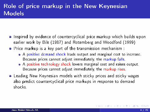
Role of price markup in the New KeynesianModels
Inspired by evidence of countercyclical price markup which builds upon
earlier work by Bils (1987) and Rotemberg and Woodford (1999)
Price markup is a key part of the transmission mechanism :
A positive demand shock leads output and marginal cost to increase.Because prices cannot adjust immediately, the markup falls.A positive technology shock lowers marginal cost and raises output.Because prices cannot adjust immediately, the markup rises.
Leading New Keynesian models with sticky prices and sticky wages
also predict countercyclical price markups in response to demand
shocks.
Jean Blaise Nlemfu M. 4 / 39
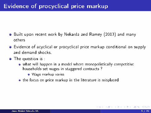
Evidence of procyclical price markup
Built upon recent work by Nekarda and Ramey (2013) and many
others
Evidence of acyclical or procyclical price markup conditional on supply
and demand shocks.
The question is :what will happen in a model where monopolistically competitivehouseholds set wages in staggered contracts ?
Wage markup varies
the focus on price markup in the literature is misplaced
Jean Blaise Nlemfu M. 5 / 39

What This Paper Does
Analyzes markup cyclicality using a medium-scale DSGE model
Inspired by Ascari, Phaneuf and Sims (2015) which built upon earlierwork by CEE (2005)An extended version with :
Non-zero steady-state in�ation
Roundabout production structure
trend growth in IST and neutral technology
aggregate �uctuations are driven by neutral technology, MEI and
monetary policy shocks
and most importantly both price and wage markups vary
assesses how positive trend in�ation a�ects the responses of price and
wage markups to shocks
Identi�es alternative sources of price and wage markups cyclical
behavior
Jean Blaise Nlemfu M. 6 / 39
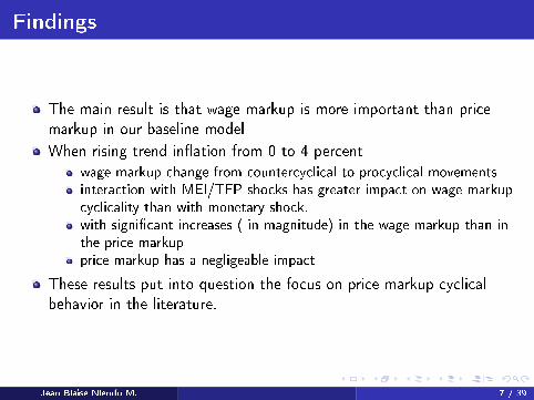
Findings
The main result is that wage markup is more important than price
markup in our baseline model
When rising trend in�ation from 0 to 4 percent
wage markup change from countercyclical to procyclical movementsinteraction with MEI/TFP shocks has greater impact on wage markupcyclicality than with monetary shock.with signi�cant increases ( in magnitude) in the wage markup than inthe price markupprice markup has a negligeable impact
These results put into question the focus on price markup cyclical
behavior in the literature.
Jean Blaise Nlemfu M. 7 / 39

Outline
1 Introduction
Background
What This Paper Does
Findings
2 The Model
Firms and Price setting
Households and Wage setting
Monetary Policy
Aggregation
3 Calibration
4 Results
Staggered Price-Setting Model
Staggered Wage - Setting Model
Staggered Price-Setting and Staggered Wage-Setting Model
5 Conclusion
Jean Blaise Nlemfu M. 8 / 39
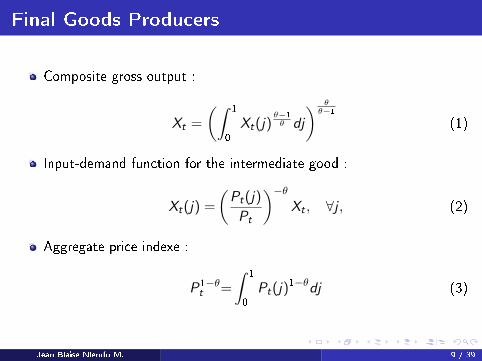
Final Goods Producers
Composite gross output :
Xt =
(∫1
0
Xt(j)θ−1
θ dj
) θθ−1
(1)
Input-demand function for the intermediate good :
Xt(j) =
(Pt(j)
Pt
)−θXt , ∀j , (2)
Aggregate price indexe :
P1−θt =
∫1
0
Pt(j)1−θdj (3)
Jean Blaise Nlemfu M. 9 / 39

Intermediate Producers
The production function for a typical intermediate producer j :
Xt(j) = max
{AtΓt(j)
φ(Kt(j)
αLt(j)1−α)1−φ
−ΥtF , 0
}, (4)
F is a �xed cost, and production is required to be non-negative.
Υt is a growth factor and F is chosen to keep pro�ts zero along a
balanced growth path.
At follows a process with both a trending and stationary component :
At = AtAτt , (5)
Aτt = gAAτt−1 (6)
The stochastic process driving the detrended level of technology At is
given by
At =(At−1
)ρAexp(sAu
At
), 0 ≤ ρA< 1 (7)
Jean Blaise Nlemfu M. 10 / 39

Pro�t Maximization and Price Setting
Firms set their price according to Calvo pricing
Since all updating �rms will choose the same reset price, the optimal
reset price relative to the aggregate price index is p∗t ≡P∗t
Pt.
The optimal pricing condition can be written:
p∗t =θ
θ − 1
x1,tx2,t
. (8)
The auxiliary variables x1,t and x2,t can be written recursively :
x1,t = λrtνtXt + βξpEt(πt+1)θx1,t+1, (9)
x2,t = λrtXt + βξpEt(πt+1)θ−1x1,t+1. (10)
Jean Blaise Nlemfu M. 11 / 39
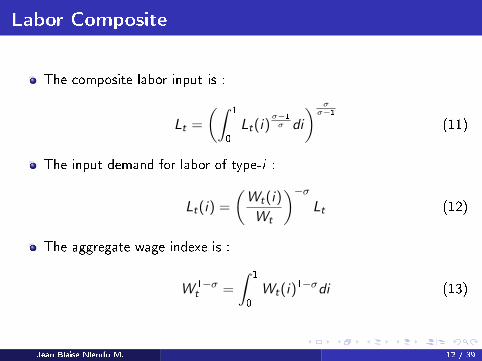
Labor Composite
The composite labor input is :
Lt =
(∫1
0
Lt(i)σ−1
σ di
) σσ−1
(11)
The input demand for labor of type-i :
Lt(i) =
(Wt(i)
Wt
)−σLt (12)
The aggregate wage indexe is :
W 1−σt =
∫1
0
Wt(i)1−σdi (13)
Jean Blaise Nlemfu M. 12 / 39
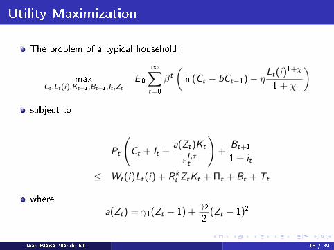
Utility Maximization
The problem of a typical household :
maxCt ,Lt(i),Kt+1,Bt+1,It ,Zt
E 0
∞∑t=0
βt(ln (Ct − bCt−1)− ηLt(i)
1+χ
1 + χ
)subject to
Pt
(Ct + It +
a(Zt)Kt
εI ,τt
)+
Bt+1
1 + it
≤ Wt(i)Lt(i) + Rkt ZtKt + Πt + Bt + Tt
where
a(Zt) = γ1(Zt − 1) +γ22
(Zt − 1)2
Jean Blaise Nlemfu M. 13 / 39
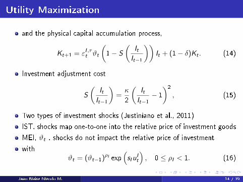
Utility Maximization
and the physical capital accumulation process,
Kt+1 = εI ,τt ϑt
(1− S
(ItIt−1
))It + (1− δ)Kt . (14)
Investment adjustment cost
S
(ItIt−1
)=κ
2
(ItIt−1− 1
)2
, (15)
Two types of investment shocks (Justiniano et al., 2011)
IST, shocks map one-to-one into the relative price of investment goods
MEI, ϑt , shocks do not impact the relative price of investment
with
ϑt = (ϑt−1)ρI exp(sIu
It
), 0 ≤ ρI < 1. (16)
Jean Blaise Nlemfu M. 14 / 39
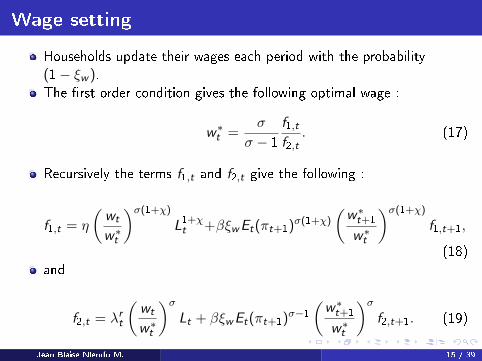
Wage setting
Households update their wages each period with the probability
(1− ξw ).
The �rst order condition gives the following optimal wage :
w∗t =σ
σ − 1
f1,tf2,t
. (17)
Recursively the terms f1,t and f2,t give the following :
f1,t = η
(wt
w∗t
)σ(1+χ)L1+χt +βξwEt(πt+1)σ(1+χ)
(w∗t+1
w∗t
)σ(1+χ)f1,t+1,
(18)
and
f2,t = λrt
(wt
w∗t
)σLt + βξwEt(πt+1)σ−1
(w∗t+1
w∗t
)σf2,t+1. (19)
Jean Blaise Nlemfu M. 15 / 39
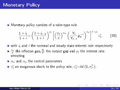
Monetary Policy
Monetary policy consists of a talor-type rule
1 + it1 + i
=
(1 + it−11 + i
)ρi [(πtπ
)απ(
Yt
Yt−1g−1Y
)αy]1−ρi
εrt . (20)
with it and i the nominal and steady state interest rate respectevelyπtπ the in�ation gap,Yt
Y the output gap and ρi the interest rate
smooting
απ and αy the control parameters
εrt an exogenous shock to the policy rule, εrt∼iid(0, σ2εr
).
Jean Blaise Nlemfu M. 16 / 39
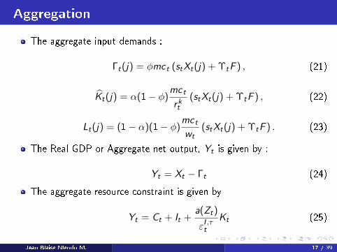
Aggregation
The aggregate input demands :
Γt(j) = φmct (stXt(j) + ΥtF ) , (21)
Kt(j) = α(1− φ)mct
rkt(stXt(j) + ΥtF ) , (22)
Lt(j) = (1− α)(1− φ)mctwt
(stXt(j) + ΥtF ) . (23)
The Real GDP or Aggregate net output, Yt is given by :
Yt = Xt − Γt (24)
The aggregate resource constraint is given by
Yt = Ct + It +a(Zt)
εI ,τtKt (25)
Jean Blaise Nlemfu M. 17 / 39
Outline
1 Introduction
Background
What This Paper Does
Findings
2 The Model
Firms and Price setting
Households and Wage setting
Monetary Policy
Aggregation
3 Calibration
4 Results
Staggered Price-Setting Model
Staggered Wage - Setting Model
Staggered Price-Setting and Staggered Wage-Setting Model
5 Conclusion
Jean Blaise Nlemfu M. 18 / 39

Calibration
Shock and Non-Shock Parameters borrowed from Ascari, Phaneuf and
Sims (2015)
Table: Non-Shock Parameters
β δ α η χ b κ γ20.99 0.025 1/3 6 1 0.7 3 0.05
θ σ ξp ξw φ ρi απ αy
6 6 0.66 0.66 0.61 0.8 1.5 0.2
Table: Shock Parameters
gA gI ρr sr ρI sI ρA sA1.00221−φ 1.0047 0 0.0020 0.95 0.0272 0.95 0.0029
Jean Blaise Nlemfu M. 19 / 39

Moments
Moments borrowed from Ascari, Phaneuf and Sims (2015)
Table: Moments
E (∆Y ) σ(∆Y ) σ(∆I ) σ(∆C ) ρ1(∆Y )
Model 0.0057 0.0078 0.0247 0.0048 0.539
Data (0.0057) (0.0078) (0.0202) (0.0047) (0.363)
σ(Y hp) σ(Chp) σ(I hp) σ(π) ρ1(π)Model 0.0169 0.0089 0.0555 0.0064 0.892
Data (0.0162) (0.0086) (0.0386) (0.0064) (0.907)
Jean Blaise Nlemfu M. 20 / 39
Outline
1 Introduction
Background
What This Paper Does
Findings
2 The Model
Firms and Price setting
Households and Wage setting
Monetary Policy
Aggregation
3 Calibration
4 Results
Staggered Price-Setting Model
Staggered Wage - Setting Model
Staggered Price-Setting and Staggered Wage-Setting Model
5 Conclusion
Jean Blaise Nlemfu M. 21 / 39
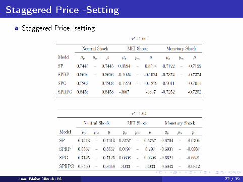
Staggered Price -Setting
Staggered Price -setting
Jean Blaise Nlemfu M. 22 / 39

Staggered Wage -Setting
Staggered wage -setting
Jean Blaise Nlemfu M. 23 / 39
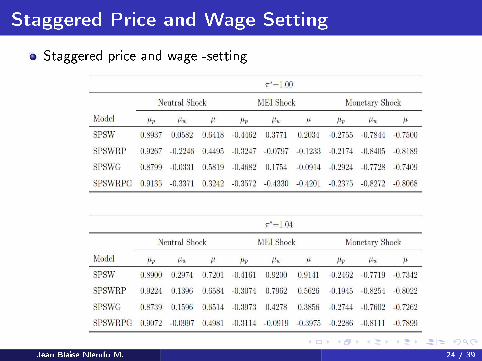
Staggered Price and Wage Setting
Staggered price and wage -setting
Jean Blaise Nlemfu M. 24 / 39

Outline
1 Introduction
Background
What This Paper Does
Findings
2 The Model
Firms and Price setting
Households and Wage setting
Monetary Policy
Aggregation
3 Calibration
4 Results
Staggered Price-Setting Model
Staggered Wage - Setting Model
Staggered Price-Setting and Staggered Wage-Setting Model
5 Conclusion
Jean Blaise Nlemfu M. 25 / 39
Conclusion
This paper analyzes markups cyclical behavior in a positive trend
in�ation medium-scale DSGE model
in a Staggered price-setting and staggered wage-setting model with
imperfect competition and trend in�ation rising from 0 to 4 percent,
wage markup is more important than price markup
The focus on the price markup in the literature is misplaced
More resarch is needed on the role of the wage markup
Jean Blaise Nlemfu M. 26 / 39
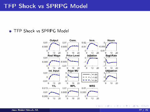
TFP Shock vs SPRPG Model
TFP Shock vs SPRPG Model
Jean Blaise Nlemfu M. 27 / 39
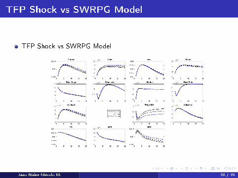
TFP Shock vs SWRPG Model
TFP Shock vs SWRPG Model
Jean Blaise Nlemfu M. 28 / 39
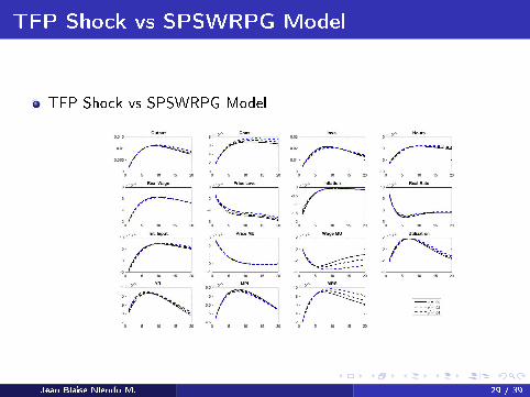
TFP Shock vs SPSWRPG Model
TFP Shock vs SPSWRPG Model
Jean Blaise Nlemfu M. 29 / 39

MEI Shock vs SPRPG Model
MEI Shock vs SPRPG Model
Jean Blaise Nlemfu M. 30 / 39

MEI Shock vs SWRPG Model
MEI Shock vs SWRPG Model
Jean Blaise Nlemfu M. 31 / 39
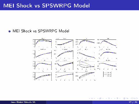
MEI Shock vs SPSWRPG Model
MEI Shock vs SPSWRPG Model
Jean Blaise Nlemfu M. 32 / 39
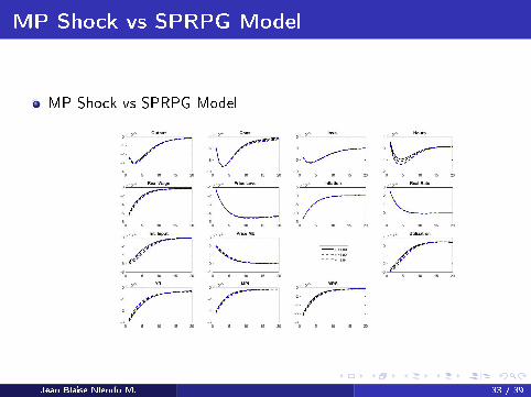
MP Shock vs SPRPG Model
MP Shock vs SPRPG Model
Jean Blaise Nlemfu M. 33 / 39
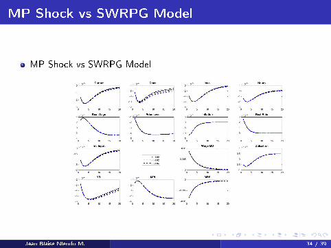
MP Shock vs SWRPG Model
MP Shock vs SWRPG Model
Jean Blaise Nlemfu M. 34 / 39
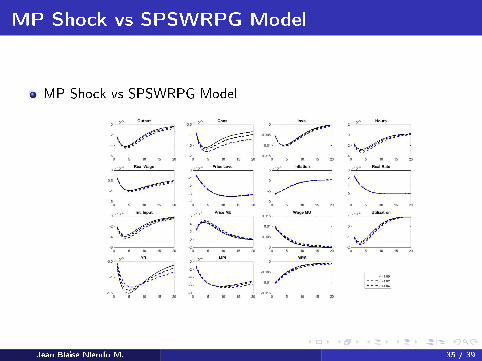
MP Shock vs SPSWRPG Model
MP Shock vs SPSWRPG Model
Jean Blaise Nlemfu M. 35 / 39

MP Shock vs SPSWRPG Model
MP Shock vs SPSWRPG Model
Jean Blaise Nlemfu M. 36 / 39

Staggered Price -Setting (FD �ltered)
Staggered Price -setting
Jean Blaise Nlemfu M. 37 / 39

Staggered Wage -Setting (FD �ltered)
Staggered wage -setting
Jean Blaise Nlemfu M. 38 / 39

Staggered Price and Wage Setting (FD �ltered)
Staggered price and wage -setting
Jean Blaise Nlemfu M. 39 / 39


