The Dan Snyder Problem: The Current State of the ... · The Current State of the Washington...

The Dan Snyder Problem: The Current State of the

Washington Redskins How a simple change in ownership managed to

change the entire trajectory of a National Football League franchise

Eliana Rae Eitches

4/26/2012

Eitches 1

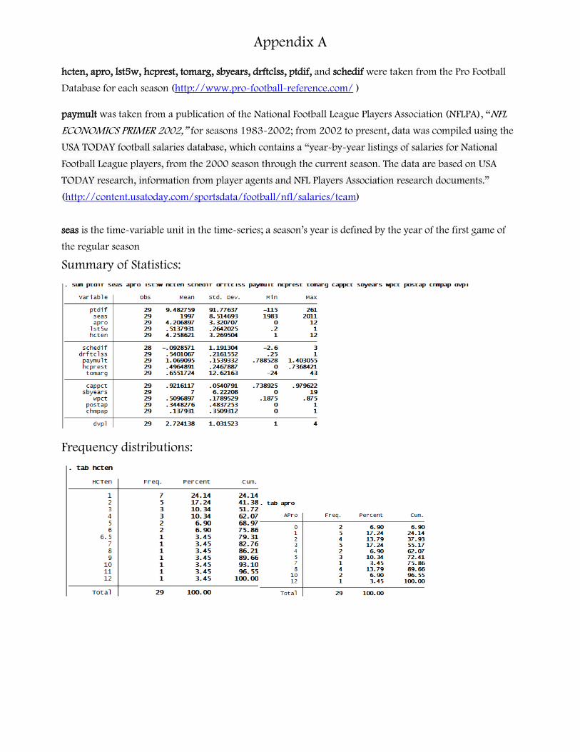
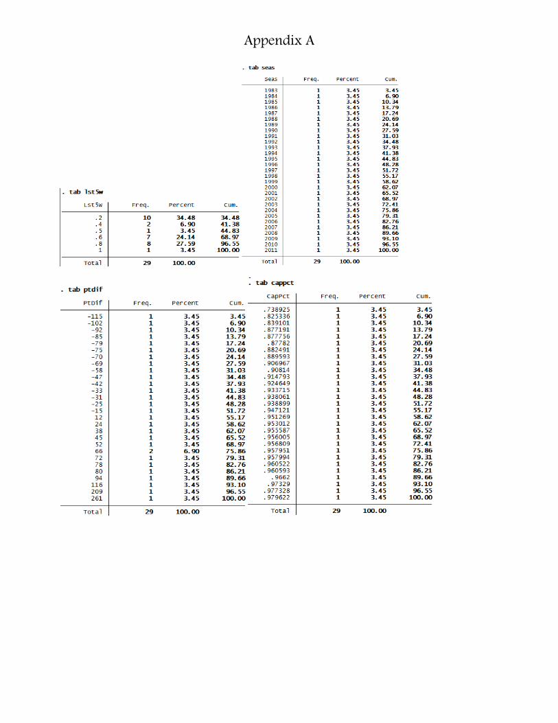
Although the Washington Redskins have not received the number one seed in the National Football Conference (NFC) of the National Football League (NFL) since the 1991 season, coincidentally the last season the team won a Super Bowl, Redskins owner since 1997, Daniel Snyder, received the top seed in the 2011 Athalon Sports’ “Worst Football Owners Bracket.”i In 2010, Washington City Paper writer and lifelong Redskins fan, Dave McKenna, wrote an article entitled “The Cranky Redskins Fan’s Guide to Dan Snyder: From A to Z (for Zorn), an encyclopedia of the owner’s many failings,” prompting Snyder to sue the paper and McKenna for “libel and defamation;” billionaire Snyder sought $2 million in “general damages” until he eventually dropped the lawsuit.ii Snyder has been criticized for rash hiring (and subsequently firing) decisions, overspending on “big-name” free agents, and inflating fan costs. Although seemingly a poor owner, Snyder remains an exceptional business man: while purchasing the Redskins for $800 million, the franchise is now worth $1.55 billion to rank as the second most valuable NFL team and fourth most valuable sports franchise worldwide.iii This paper aims to ascertain whether the Snyder criticism is valid by examining data on the Washington Redskins from the 1983 season, when the team was owned by Jack Kent Cooke, to 2011. This paper posits that a time-series regression model (causal path diagram, data sources, and frequency distributions for variables in Appendix A) with the year of the season (var:seas) as the time-variable unit (time period beginning with the 1983 season and ending with the 2011 season) will display a precipitous decline in team quality as the year increases: the poor health and eventual death of Cooke preceding the purchase of the team by Snyder will manifest as an overall negative trend in team quality, influenced by ten exogenous variables representing franchise management, quality of players, capability of coaches, and fan support.

Overall team quality, the endogenous variable in the model, is quantified by the team’s point differential (var: ptdif; total points scored by the team – total points scored by opponents) throughout the 16 regular season games; a quality team is the culmination of a multitude of factors, but the best teams are those that obliterate all competition on a consistent basis. Franchise management is represented by four variables: years since the last Super Bowl appearance (var: sbyears), draft class quality (var:drftclss), pay multitude (var:paymult). When a team is run by effective managers, they usually accrue the designation of a “dynasty” because of their perennial post-season appearances and victories with the most dynastic franchises earning frequent Conference championships and, resultantly, trips to the Super Bowl. The Detroit Lions are the only franchise in the NFL continuously in operation during the Super Bowl era (since 1965) to have never reached the Super Bowl, due in part to notorious managerial incompetence; incidentally, in 2007, the Lions became the first franchise to lose all 16 regular season games in history. Between 2001 and 2011, the New England Patriots reached the Super Bowl four times and, in 2007, became the first team to be undefeated in the 16 regular season games; accordingly, the Patriots are well-known for their superb personnel decisions and management. A hallmark of good management is recognizing and drafting quality players that remain with the team, contributing to sustained success. drftclss is given by the percentage of players taken in the first five rounds of the NFL draft occurring four years prior to a given season (ex. for 1983, the 1979 NFL draft) that remain on the squad; the four-year period was chosen because draftees typically have either four- or five-year contracts with opt-out clauses in the third year to eliminate high salary payments to proven ineffective players. Salary management, especially in the era of the salary cap, is crucial for effective management. paymult is the total player expenditure (base salary and bonuses) for the team at the start of the season divided by the league average. Higher player expenditures have two primary sources: bonuses to free agent acquisitions (indicating that members of the squad had to be released in order to meet salary cap requirements without the guarantee that a star player on a different team will transition efficiently and be productive in the new system) and high veteran salaries (veterans have higher minimum salaries yet are typically less athletic and have a shorter shelf-life than younger players).

Player quality is given by three variables: turnover margin (var:tomarg; number of takeaways – giveaways/turnovers in a given season) because a high turnover margin indicates proficiency on both offense (few interceptions and other miscues) and defense (adept at limiting opportunities for the other

Eitches 2

team to score); the win percentage of the last five games of the regular season (var: lst5w) as it indicates that players likely retained both their overall health and a desire to win during the season; and the number players selected to the All-Pro team during the previous three seasons (var:apro; the season of 1983 would have an apro equal to the number of players designated All-Pro at the culmination of the 1980, 1981, and 1982 seasons) since All-Pro designations are bestowed following a season. Coaching competence is represented by three variables: schedule difficulty (var:schedif; average strength of opposing teams based on their win-loss records for the season) as superior coaches formulate their game plan by dissecting the information about an opponent to play to their team’s strengths; number of continuous seasons under a given head coach (var:hcten; a coach entering their first season with the team receives a value of 1) since intimate acquaintance with their players will foster both trust and resourceful utilization of available personnel; and a head coach’s lifetime winning percentage prior to entering a given season (var: hcprest; a first-year head coach receives a value of 0) as prestigious coaches should have their prior successes carry from team-to-team and from season-to-season. Fan approval is given by average capacity of the stadium filled throughout the eight home games in a season (var:cappct) because rational disenchanted fans will not pay premium dollars to see a team; because of floundering capacity percentages, Snyder removed 9,704 seats from the Redskins stadium (FedEx Field) prior to the 2011 season to amount in an artificially high cappct value for that season in the data.iv Aside from the foreseeable outlier year in cappct, all variables are expected to have high face validity for the measures; the unit of analysis for the paper is the Washington Redskins.

Our time series model aims to uncover the stochastic process underlying trends in team quality (through ptdif) observed between the 1983 and 2011 seasons, allowing for inferences about the future team quality to be made. Graphing ptdif over time (Appendix B) displays a cyclical pattern with an overall downward trajectory; ergo, further tests must be conducted to determine whether our model is a stationary or nonstationary. A stationary stochastic process would signify that ptdif is “time-invariant”: ptdif exhibits constant variance and autovariance between time lags, cyclically fluctuating around and reverting to its mean, so its expression in one time period does not have an independent causal effect on the next (ptdif’s disturbance terms are uncorrelated). On the contrary, a nonstationary stochastic process involves a time-varying mean and/or a time-varying variance, denoting that a variable’s inconsistent behavior between time periods queries the validity of predictive forecasting. Thus, if random variables (encompassed by the disturbance term) within a given time lag trigger a “random shock” in ptdif unexplained by the model, two classical linear regression model assumptions (CLRM) about disturbance terms are violated: 1) constant variance, because disturbance term variance changes in response to the new values created by the shock, and 2) uncorrelation, as ptdif in a given time lag is determined by the value ptdif assumes in the previous time lag and as “shock” distorts ptdif’s expected disturbance value, each successive time lag iteration of ptdif’s disturbance term (starting with the shock’s time period and continuing for infinite periods) will be serially correlated with a proportion of the original shock-influenced disturbance term. Serial correlation among a variable’s disturbance terms in a nonstationary time series follows either a negative trend (negative serial correlation), implying vacillation between high and low values of a variable between adjacent time lags; or a positive trend (positive serial correlation), implying that a disturbance term’s positivity or negativity in a given period configures an identical unidirectional movement in a variable’s expression until a “shock” interpolates a later time lag.

Casinos can consistently profit from football wagers because of serial autocorrelation: even a highly predictive model cannot confidently estimate the magnitude of causal effect conferred by a disturbance term modified by “shocks” that, by definition, arise according to the randomness of chance. Consequently, only a stationary time series (exhibiting constant variance, mean, and covariance) abides by CLRM assumptions, signifying that inferences made through the interpretation of Ordinary Least Squares Regression (OLS) parameter estimations are valid. OLS on a non-stationary model yields unbiased and consistent parameter estimation; however, increased variability in the disturbance term causes OLS estimations to be inefficient predictors of a variable’s actual value. Accordingly, the model of the paper

Eitches 3

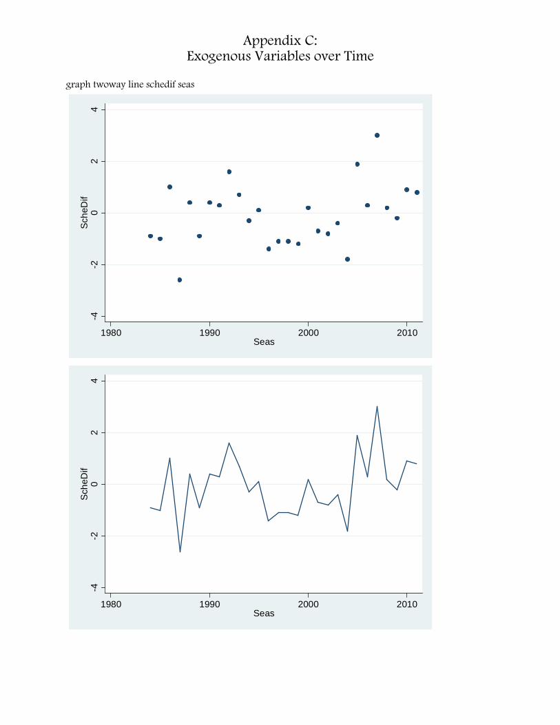
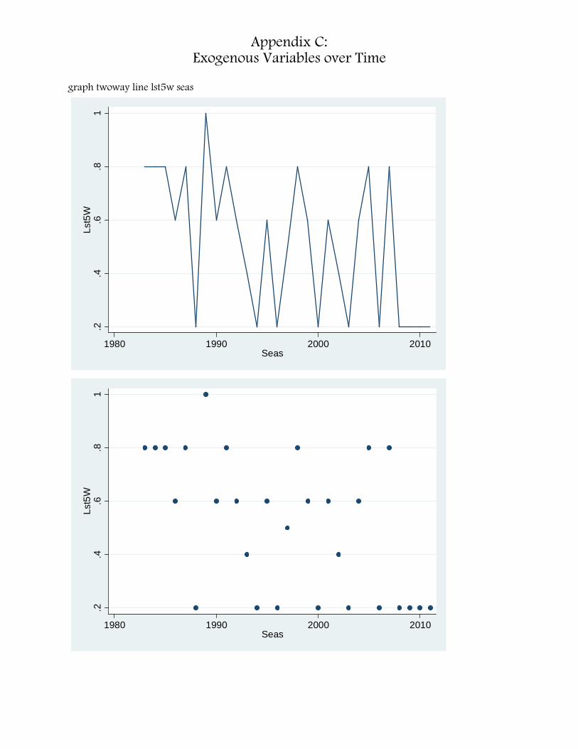
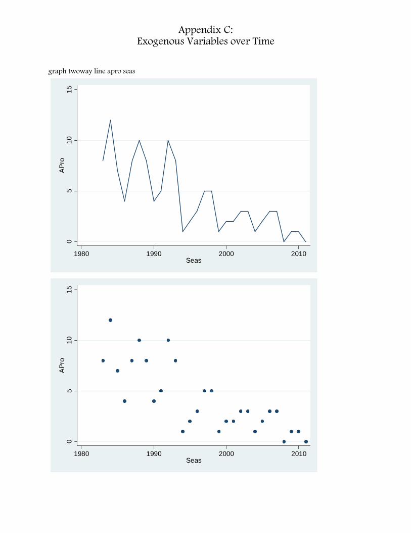
must first be evaluated for stationarity. Examining the graph of a variable over time will preliminarily suggest non-stationarity if the mean value of the variable appears to change alongside time (Appendix C); none of the variables appear to be completely time-invariant but, concurrently, trends in the data are difficult to ascertain. apro, for example, displays non-stationarity through an overall tendency to decrease with time; its oscillation between high and low values in adjacent time lags may signify stationarity as its mean value could be constant throughout the time series. cappct is the variable most likely to exhibit stationarity as it assumes relatively constant values throughout time.

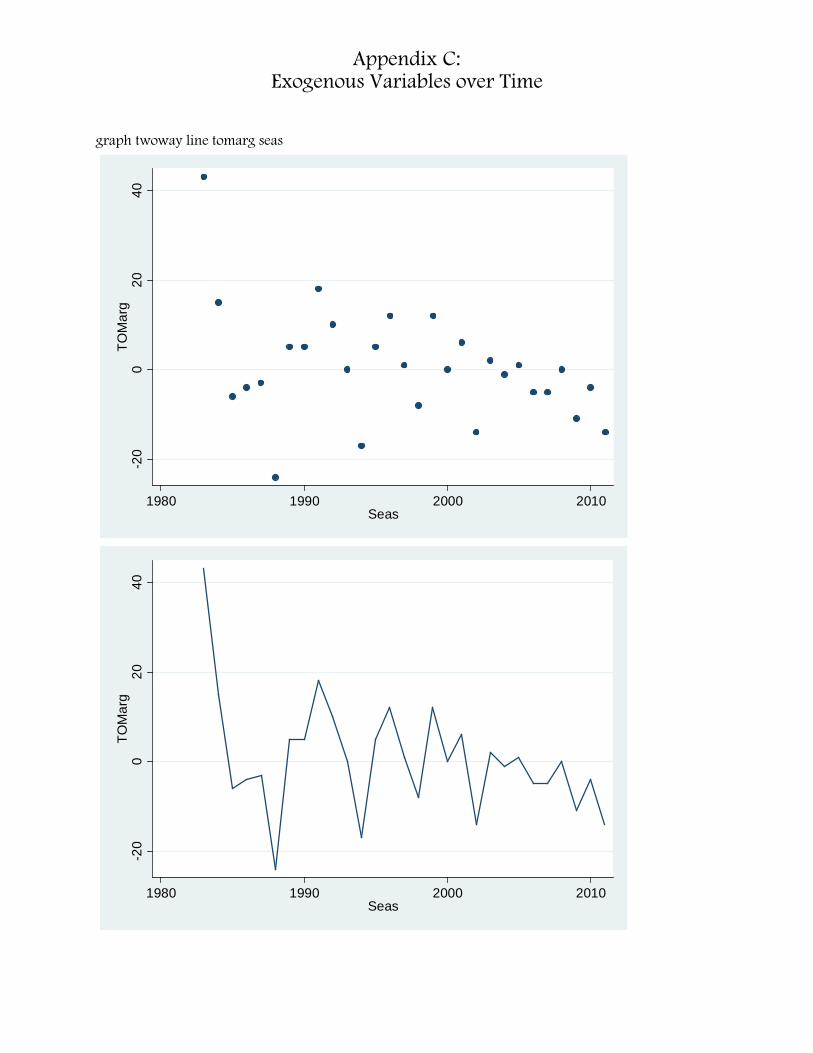
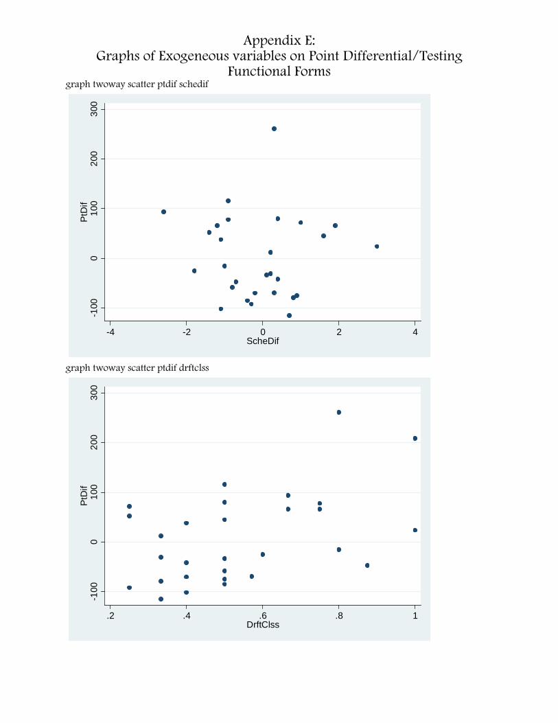
Covariance, as presented in a zero-order correlation matrix (Appendix D) to elucidate the magnitude and direction with which any two variables change together; a covariance of 0 would signify a time-invariant model that is intrinsically stationary. Covariance coefficients “-1” and “1” signal perfect serial correlation in the direction of the coefficient. With all non-zero coefficients that assume the proposed directionality of the relationships, the data is less likely to be classified as “stationary:” an increase in apro, lst5w, hcten, drftclss, hcprest, tomarg, and cappct appear to increase ptdif while increases in schedif, paymult, and sbyears result in a decrease. Scatterplots of the exogeneous variables on ptdif (Appendix E) lack an indication that model variables would significantly benefit from adopting a different functional form; as specification error does not impart its effect on the model, it cannot indicate impure serial correlation. Moreover, much of the sample was gleaned from a dataset issued by the National Football League Players Union (NFLPA) or is of public team record, conveying the legitimacy of the source data. An outlying point is perceptible across all graphs, galvanizing the belief that its degree of distinction likens it to a leverage point: the 1991 Redskins, considered one of the top 10 greatest teams in the history of the NFL by amassing the second highest point differential ever at +261; 52 points greater than our model’s next highest total)v, decreased the model’s accuracy yet exemplified its theoretical purpose, causing it to be inextricable from the data. The 1983 Redskins, setting an NFL record for number of turnovers (tomarg=43), will similarly be left in the data.

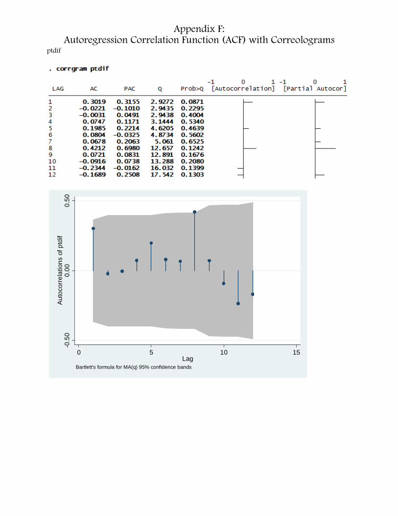
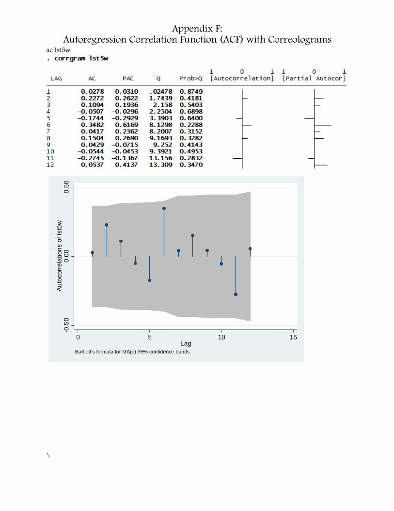
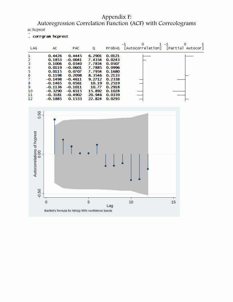
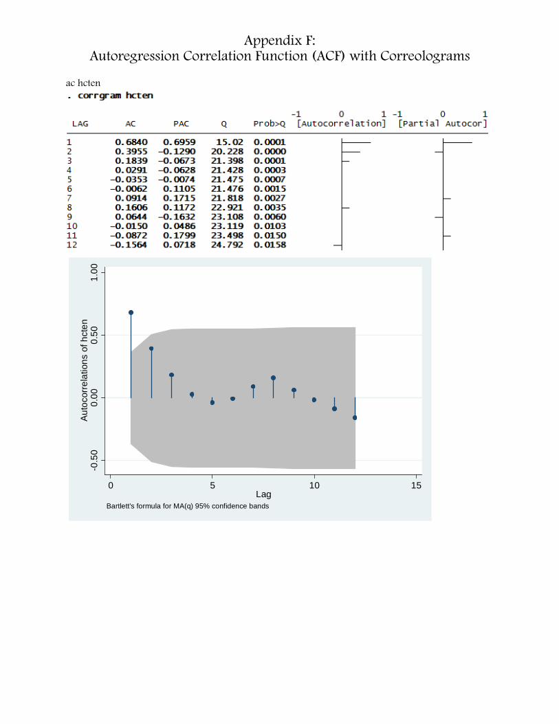
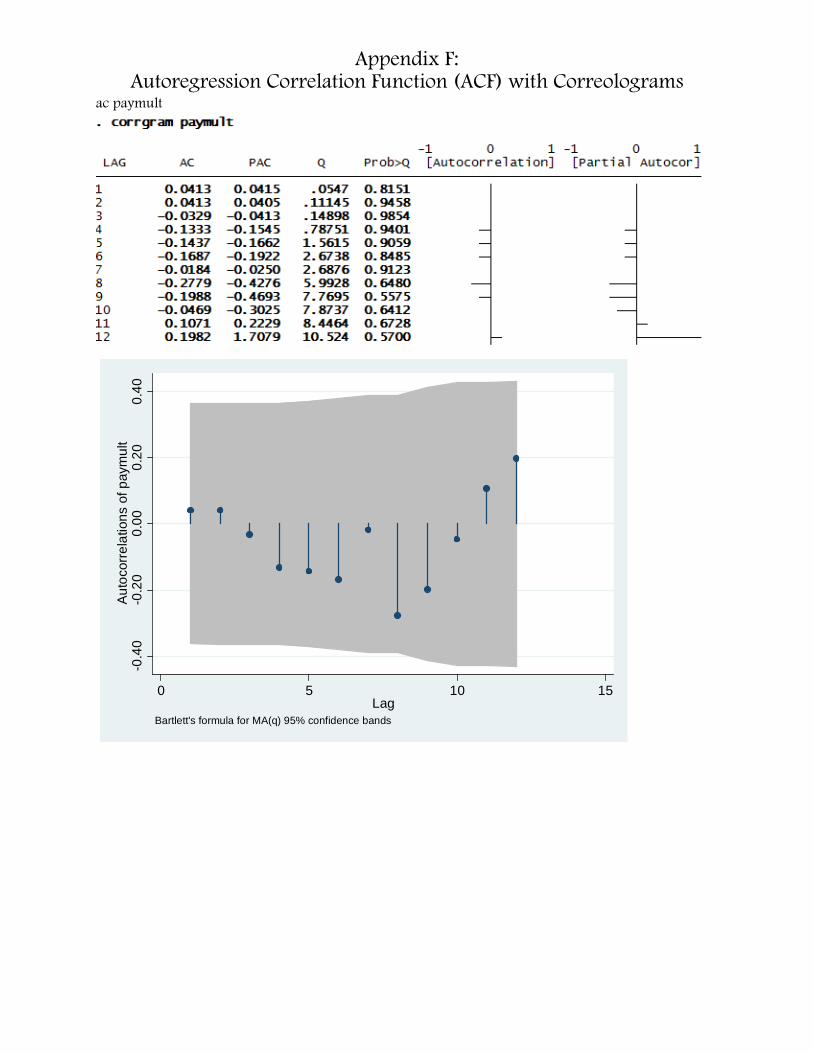
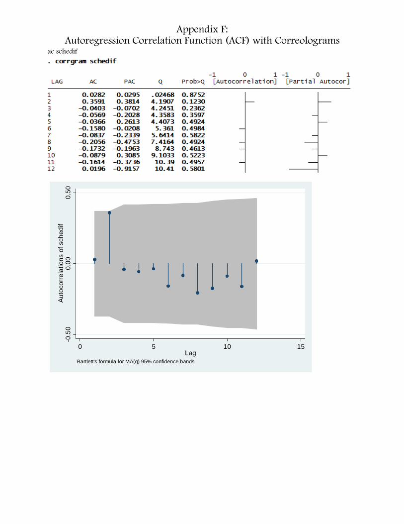
Without the threat of specification error, a first-order autoregressive scheme (AR (1) may be able to transform serially correlated data if possessing sufficiently high autocorrelation coefficient; although its variance estimations will likely differ from those presented by OLS, the problems posed by biased standard errors (leading to inaccurate hypothesis testing) are ameliorated. AR(1) remedies the forecasting barriers activated by indeterminable disturbance terms, characteristic in non-stationary models, performing a “first-difference transformation” to a stationary model: removing stochastic trends by expressing a disturbance term in a given time period as a linear function of the term in the previous period. As correlation coefficients within the matrix profess an absolute value < 1, the correlogram representing a variable’s autocorrelation function (AFC) would illustrate decay over time that eventually converges to zero (a white noise error term with constant variance, normal distribution, zero mean, and serial uncorrelation). Appendix F displays AFC and corresponding correlograms for each variable with a time lag equal to one season (lag=1), revealing the stationarity and the covariance within time period-specific iterations of a variable. The correlograms for lst5w, schedif, paymult, cappct, and tomarg do not display a statistically significant (at confidence level α=.05) difference between the residuals of those variables and 0 serial correlation (random white noise error) at any time lag, thus, their time series is stationary. Statistically significant autocorrelation (at α=.05) is found for all time lags of hcten, apro, and sbyears. drftclss exhibits statistically significant deviation (α=.05) from 0 mean serial correlation in its error terms except in the 1st and 4th lag, hcprest is significantly statistically different (α=.05) during its first and last pair of lags, while ptdif is not significantly different with 95% confidence. Stationary trends indicated in the corrollograms for hcten, sbyears,

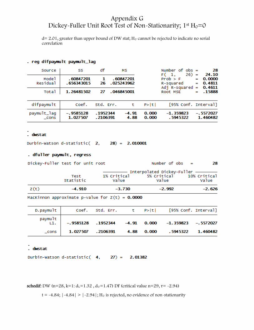
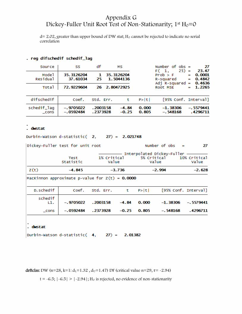
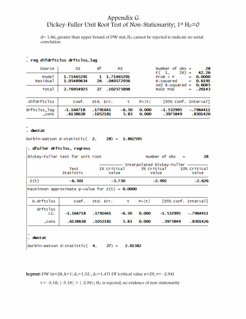
Since only four variables indicate definite stationarity and the remainder retain an implication of serially correlated disturbance terms, the unit root test (a model of a completely random stochastic trend) is utilized to unearth the model’s stationarity before inferences can be made. The test, named the Dickey-Fuller (DF) test (Appendix G), encompasses three null hypotheses: 1) a variable is a random walk (random variances concentrated within a period), 2) a variable is a random walk with drift (nonstationary with a

Eitches 4

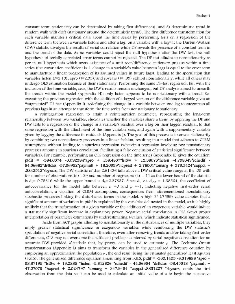
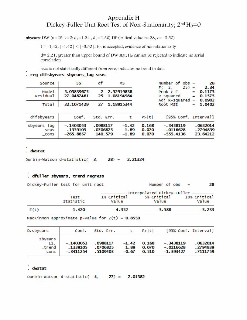
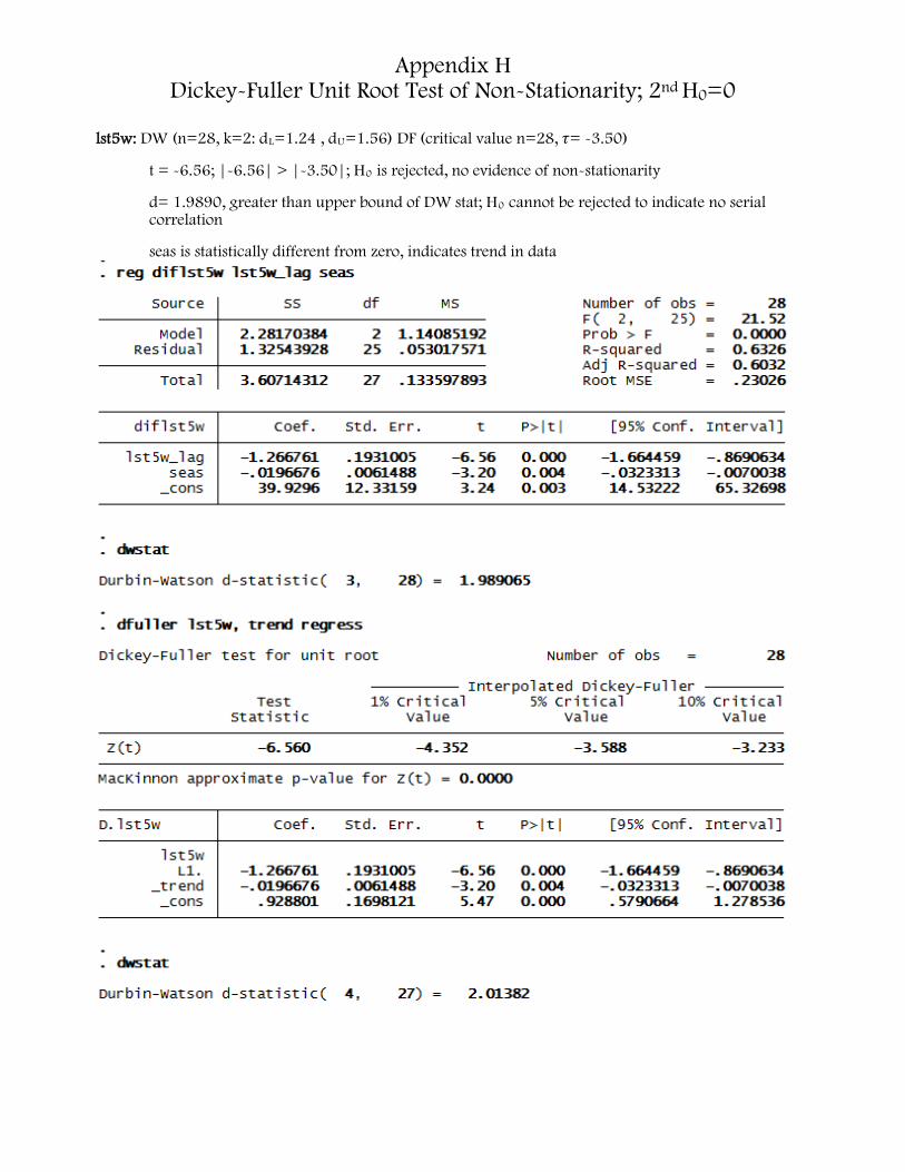
constant term; stationarity can be determined by taking first differences), and 3) deterministic trend in random walk with drift (stationary around the deterministic trend). The first difference transformation for each variable manifests critical data about the time series by performing tests on s regression of the difference term (between a variable before and after a lag) on a variable with a lag=1: the Durbin-Watson (DW) statistic divulges the results of serial correlation while DF reveals the presence of a constant term in and the trend of the data. As no variables could reject the null hypothesis after the DW test; the null hypothesis of serially correlated error terms cannot be rejected. The DF test alludes to nonstationarity as per its null hypothesis which avers existence of a unit root/difference stationary process within a time series (the covariation coefficient is 1, change in a variable’s value between lags is equal to the error term to manufacture a linear progression of its assumed values in future lags), leading to the speculation that variables hcten (t=2.13), apro (t=2.33), and sbyears (t= .99) exhibit nonstationarity, while all others may undergo OLS estimation because of their stationarity. Performing the same DF-test regression but with the inclusion of the time variable, seas, the DW’s results remain unchanged, but DF analysis aimed to unearth the trends within the model (Appendix H): only hcten appears to be nonstationary with a trend. Re-executing the previous regression with the addition of a lagged version on the difference variable gives an “augmented” DF test (Appendix I), redefining the change in a variable between one lag to encompass all previous lags in an attempt to transform the time series from nonstationary to stationary.

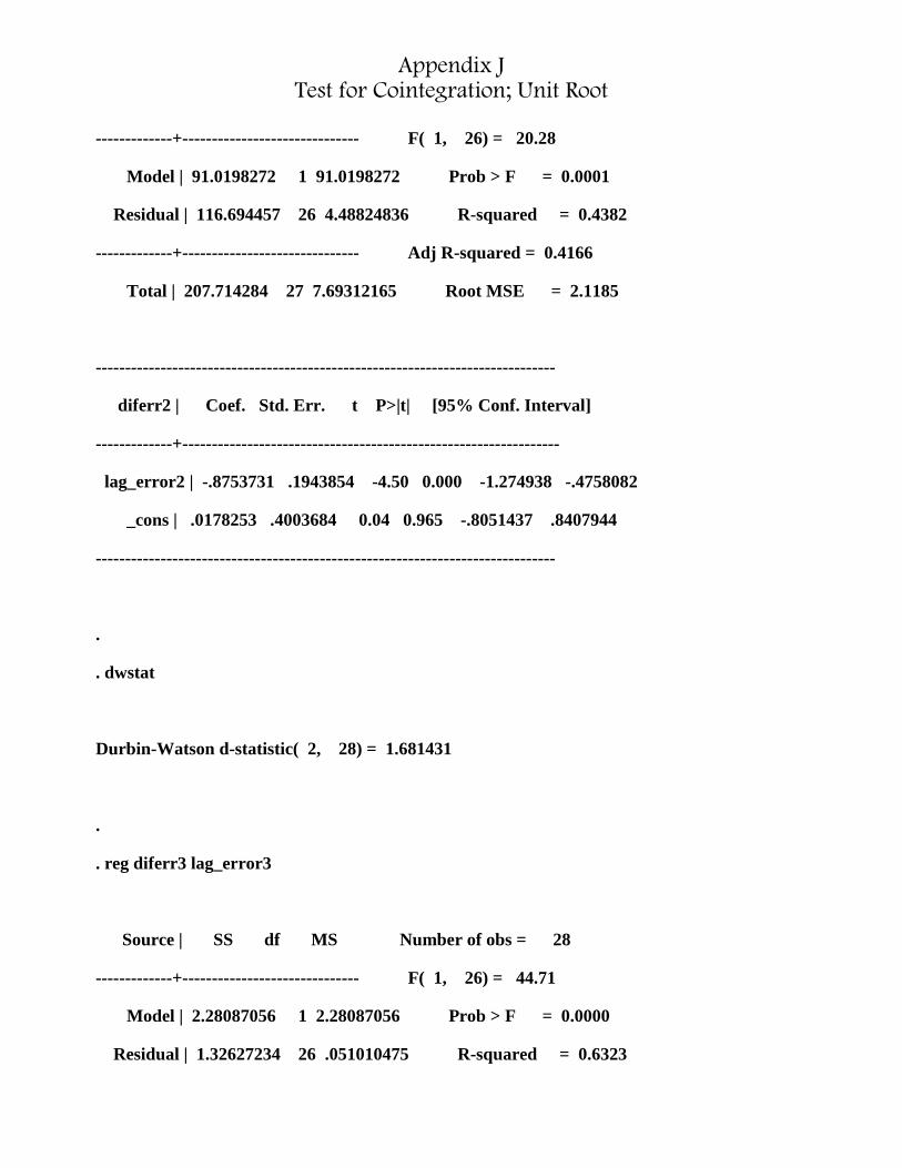
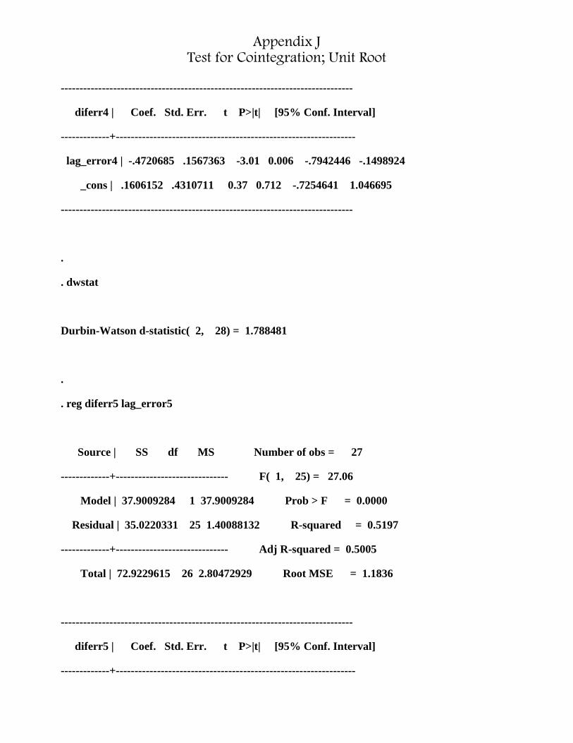
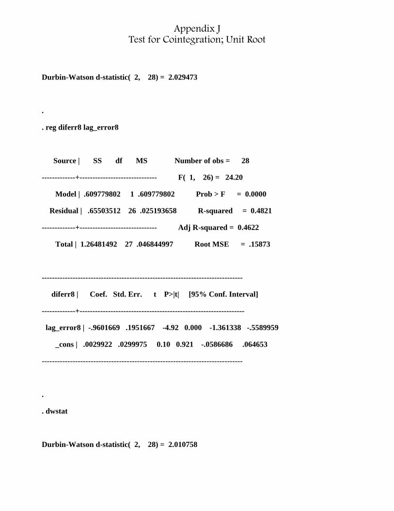
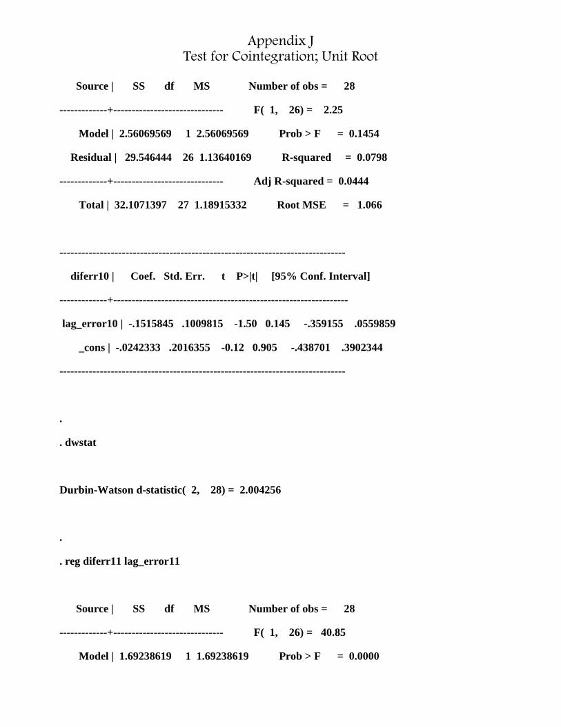
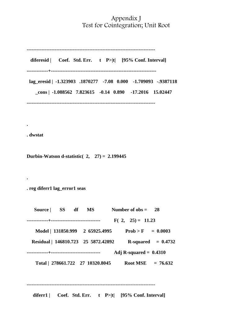
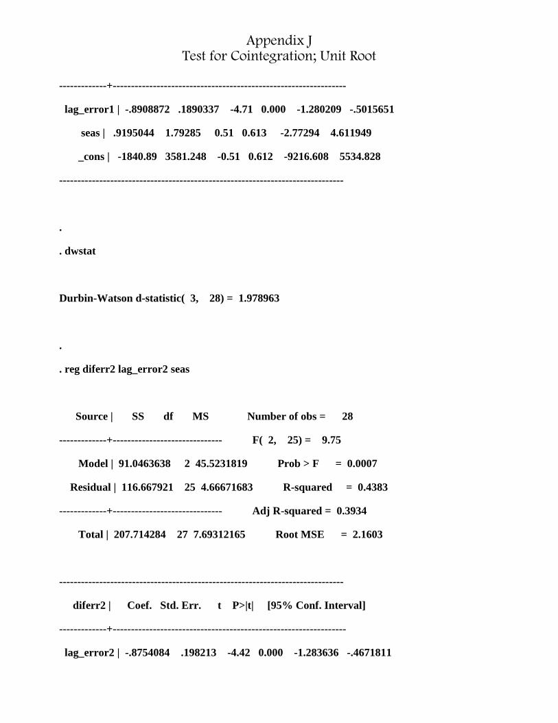
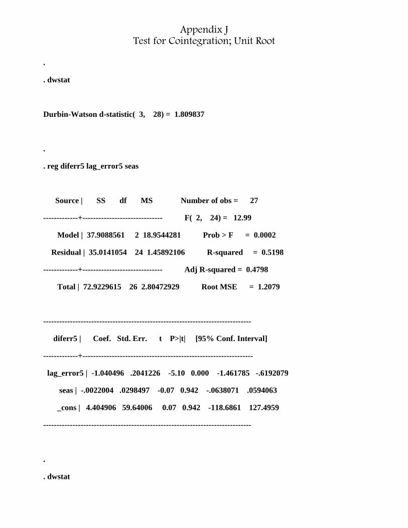
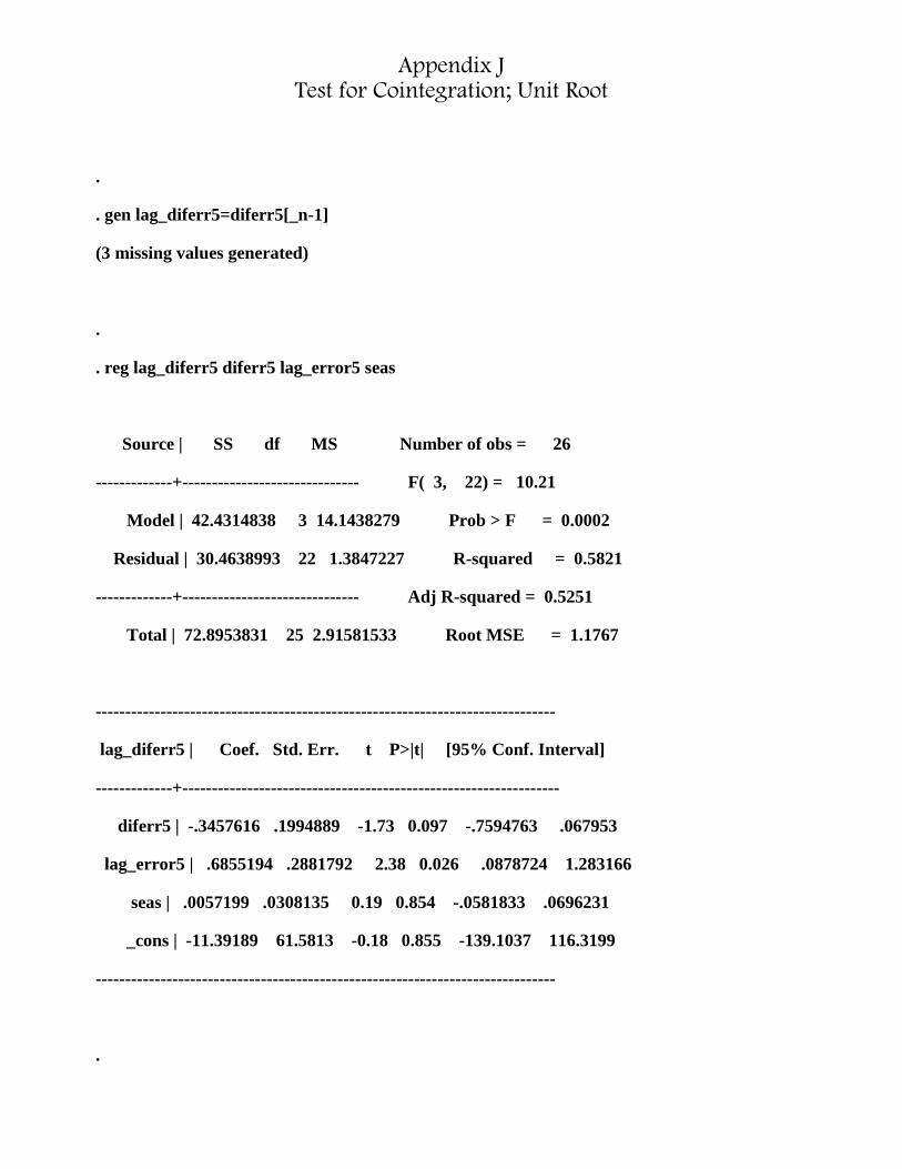
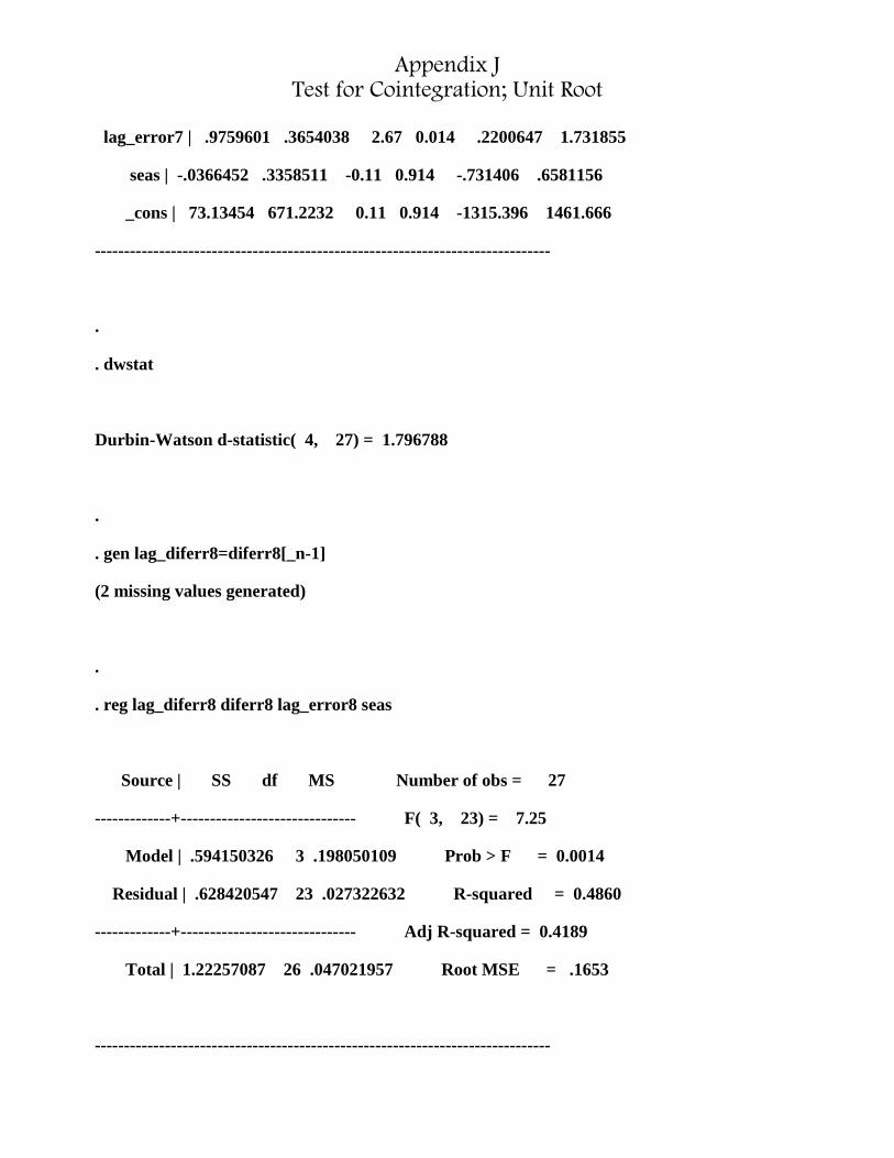
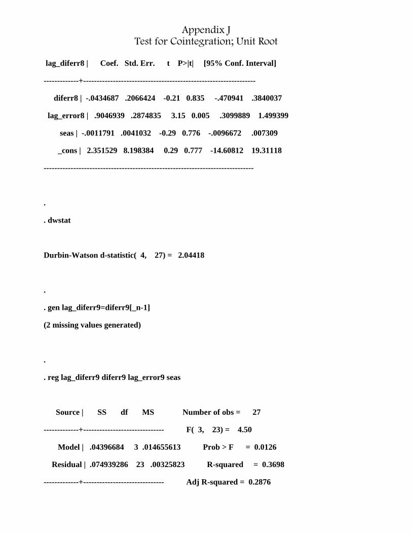
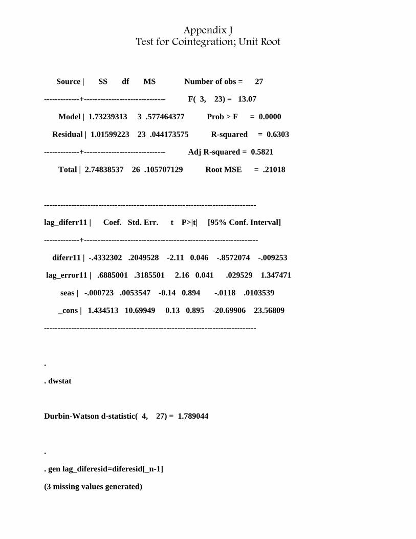
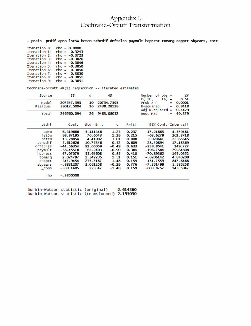
A cointegration regression to attain a cointengration parameter, representing the long-term relationship between two variables, elucidates whether the variables share a trend by applying the DF and DW tests to a regression of the change in a variable’s residual over a lag on their lagged residual, to that same regression with the attachment of the time variable seas, and again with a supplementary variable given by lagging the difference in residuals (Appendix J). The goal of this process is to create stationarity by combining two nonstationary processes in a linear fashion, resulting in a model that adheres to CLRM assumptions without leading to a spurious regression (wherein a regression involving two nonstationary processes amounts in spurious correlation, facilitating a false conclusion of statistical significance between variables). For example, performing an OLS regression on the time series (Appendix K) gives the equation: ptdif = -364.0574 -3.092384*apro + 136.4837*lst5w + 12.58075*hcten -4.798549*schedif -84.56662*drftclss -57.96952*paymult + 18.20999*hcprest + 2.76001*tomarg + 379.3424*cappct + .8842512*sbyears. The DW statistic of dOLS 2.61436 falls above a DW critical value range at the .05 with for number of observations (n) =29 and number of regressors (k) = 11 as the lower bound of the statistic is dL= 0.75316 while the upper bound is dU=2.27837. Since dU >4-dOLS = 1.38564, the coefficient of autocovariance for the model falls between ρ =0 and ρ =-1, indicting negative first-order serial autocorrelation, a violation of CLRM assumptions, consequences from aforementioned nonstationary stochastic processes linking the disturbance terms in the model. A high R2 (.7559) value denotes that a significant amount of variation in ptdif is explained by the variables delineated in the model, so it is highly unlikely that the transformation of a given variable or the addition of an exogenous variable would induce a statistically significant increase in explanatory power. Negative serial correlation in OLS skews proper interpretation of parameter estimations by underestimating t-values, which indicate statistical significance. Aside from ACF graphs alluding to nonstationarity in the disturbances of multiple variables, they imply greater statistical significance in exogenous variables while reinforcing the DW statistic’s speculation of negative serial correlation; therefore, even after removing trends and/or taking first-order differences, OLS may not overcome the sufficient problems conferred by serial negative correlation for an accurate DW-provided d-statistic that, by proxy, can be used to estimate ρ. The Cochrane-Orcutt transformation (Appendix L) aims to transform the variables in the generalized difference equation by employing an approximation the population ρ , the end result being the estimated generalized least squares (EGLS). The generalized difference equation amounting from EGLS, ptdif = -330.1405 -6.319686 *apro + 98.87195 *lst5w + 13.2885 *hcten -5.612626 *schedif - 44.56354 *drftclss -58.45518 *paymult + 47.07079 *hcprest + 2.024797 *tomarg + 347.9454 *cappct-.8831207 *sbyears, omits the first observation from the data so it can be used to calculate an initial value of ρ to begin the successive

Eitches 5

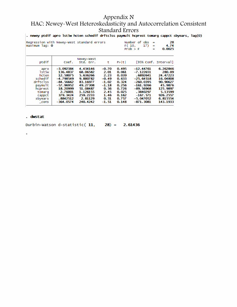
approximation of ρ for later time lags. The whole process amounts in a ρ population estimation = -.3850508, and a transformed DW statistic of 2.195050, within the boundaries mandated in a 28 =n, 10=k sample, but places d in the zone of indecision: dL=.72265, dU=2.30862. The regression also displays insignificance of parameter estimations as a result absolute values of the t statistic for every variable except for statistically significant hcten (t=3.01). The Prais-Winsten transformation (Appendix M) also involves a regression equation in difference form, subtracting a proportion=p from the value of the variable in the previous time period to appraise tits value in a given time period: ptdif = -360.2216-3.92472* apro + 112.6407*lst5w + 11.65253 *hcten -6.129222 *schedif -70.3803*drftclss -65.47841*paymult + 53.00176hcprest + 2.519868 *tomarg + 386.4624*cappct-.2144049*sbyears. Its DW statistic equals 2.326292 (dL= 0.75316 , dU=2.27837 to say with 95% confidence that the model does not reject the null hypothesis of negative serial correlation) and population parameter =-.4030286. The t-statistics for only two variables proved statistically significant: tomarg (t= 2.09) and hcten (t=2.94). In comparison with EGLS, its F-value is greater (9.18 versus 8.51), displaying the magnitude to which statistical significance within a model varies in relation to its number of observations. As sample size increases, it would logically conclude that a “full” estimated GLS (Prais-Winsten) will convergence alongside EGLS (Cochrane-Orcutt) on a specific result for population estimators. A small sample size like that of the data will exhibit a palpable difference in regression coefficient (F-statistic=8.51 with EGLS v. 9.18 with Full GLS) wherein the inclusion of the 1983 season accounted for 7.88% greater F-statistic and %1.196968 in R2 (perhaps indicating that the model estimations were nearing the end of the convergence process). Furthermore, the ρ is 4.6689% less, indicating less serial correlation in the model through less carryover between lags. Adding the 1983 to the model perhaps credits the urban legend of “Super Bowl Hangover:” wherein the great success of a Super Bowl appearance is succeeded by great team failure because of traded players, assistant coaches hired for head coaching positions elsewhere, and less effort during training camp/the preseason. Thus, it is logical to assume that a serial correlation correction method most efficient with large, like the Newey-West heteroskedasticity and autocorrelation consistent standard errors (HAC) samples, will not be an efficient predictors with a sufficiently small p value. HAC (Appendix N) gives the regression equation ptdif= -364.0574 -3.092384*apro + 136.4837 *lst5w+ 12.58075*hcten -4.798549*schedif -84.56662*drftclss -57.96952*paymult + 18.20999*hcprest + 2.76001*tomarg + 379.3424*cappct .8842512*sbyears, including three statistically significant exogenous variables yet a low F-statistic (4.74). A head coach’s number of years as the head coach (hcten) was the only variable with statistical significance across all regression models, exhibited a nonstationary process, and exhibited serial correlation (negative trend); the fact that the highest t-value for hcten was the result of the EGLS method proposes an interesting conclusion: as time increases, head coaching tenure becomes more predicative of point differential while a head coach’s lifetime win percentage does not exhibit the same trend. Perhaps, this posits, the most important factor in a team’s success is continuity: stability, not prestige, breed success. In the Dan Snyder era, though, stability has been noticeably absent at FedEx Field in all facets of team success. Reexamining the trends in variables over time, the trend mostly points downward after 1997. Accordingly, the reason for little explanatory power within the model is more the result of the unpredictability of winning and success versus the relative predictable nature of losing. The team exhibited a trend of a mostly random walk in terms of team successes and failures from 1983 to 1997, but the deterministic quality of the model from 1997 to 2011 shrouded substitutive conclusions gleaned through regression analysis. Snyder, it follows, likely the root cause of the lack of substantive conclusions forged by the model while ensuring a deterministic process downward will persist.

i http://www.athlonsports.com/nfl/worst-sports-owners-tournament-football-round-1 ii http://www.washingtoncitypaper.com/blogs/citydesk/2011/09/10/dan-snyder-drops-lawsuit-against-washington-city-paper-dave-mckenna/

http://www.athlonsports.com/nfl/worst-sports-owners-tournament-football-round-1

http://www.washingtoncitypaper.com/blogs/citydesk/2011/09/10/dan-snyder-drops-lawsuit-against-washington-city-paper-dave-mckenna/

http://www.washingtoncitypaper.com/blogs/citydesk/2011/09/10/dan-snyder-drops-lawsuit-against-washington-city-paper-dave-mckenna/

Eitches 6

iii http://www.washingtonpost.com/blogs/football-insider/post/forbes-redskins-are-4th-most-valuable-sports-franchise/2011/07/14/gIQAAr0TEI_blog.html iv http://www.washingtonpost.com/sports/redskins/redskins-say-they-were-unable-to-sell-season-tickets-for-seats-removed-from-fedex-field/2011/07/14/gIQA1vbwEI_story.html v http://sports.espn.go.com/espn/page2/story?page=super/rankings/1-20

http://www.washingtonpost.com/blogs/football-insider/post/forbes-redskins-are-4th-most-valuable-sports-franchise/2011/07/14/gIQAAr0TEI_blog.html

http://www.washingtonpost.com/blogs/football-insider/post/forbes-redskins-are-4th-most-valuable-sports-franchise/2011/07/14/gIQAAr0TEI_blog.html

http://www.washingtonpost.com/sports/redskins/redskins-say-they-were-unable-to-sell-season-tickets-for-seats-removed-from-fedex-field/2011/07/14/gIQA1vbwEI_story.html

http://www.washingtonpost.com/sports/redskins/redskins-say-they-were-unable-to-sell-season-tickets-for-seats-removed-from-fedex-field/2011/07/14/gIQA1vbwEI_story.html

http://sports.espn.go.com/espn/page2/story?page=super/rankings/1-20

Appendix A

tomarg: the difference between the number of times the Redskins ended an opponent’s possession by creating a turnover minus the number of times the Redskins turned the ball over to their opponent during the previous season

(ex. intercepted opponent passes - fumbles team lost)

apro: Number of Players selected for the All Pro 1st or 2nd team during the previous two seasons on the roster for a given season

hcten: Head coach’s tenure in Washington (where “new coach” assumes a value of 1)

lst5w: win percentage over the last five games of the season (%)

hcprest: “prestige” of the head coach, given by the lifetime winning percentage of a coach prior to entering a given season; new coaches assume the value 0

cappct percentage attended game/stadium capacity; represents overall fan enthusiasm toward team (1983, RFK Memorial Stadium, Capacity: 55,045; 1984, RFK Stadium, Capacity: 55,431; 1985-1991, RFK Stadium, Capacity: 55,750; 1997-1999, Jack Kent Cooke Stadium, Capacity: 91,704; 2000-2010, Fed-Ex Field, Capacity: 91,704; 2011-Present, Fed-Ex Field, Capacity: 82,000)

paymult: the ratio of the team’s total player expenditure (bonus + salary) in a given season to the league’s average player expenditure

sbyears: the number of seasons since the team’s last Super Bowl appearance (denoting victory in their conference’s championship game) where winning the Super Bowl in the prior season assumes a sbyears=0

drftclss: the ratio of the number of players on the roster in a given season that were drafted by the team in the first five rounds in the NFL draft occurring four seasons prior (ex. players drafted in the 2000 season that were on the roster in 2004) to the total number selected by the team in the first five rounds of the NFL draft four years prior

schedif: the predicted strength of a team’s schedule in a given season as determined by the average “strength” of all opponents as exhibited during the prior season; 0 indicates an “average” team; the algorithm is calculated by Pro Football Reference

http://www.pro-football-reference.com/blog/?p=37

ptdif: the point differential; the total number of points scored by a team throughout a given season’s 16 game schedule minus the total number of points scored against a given team by opponents in regular-season games

(points for-points against)


Appendix A

hcten, apro, lst5w, hcprest, tomarg, sbyears, drftclss, ptdif, and schedif were taken from the Pro Football

Database for each season (http://www.pro-football-reference.com/ )

paymult was taken from a publication of the National Football League Players Association (NFLPA), “NFL

ECONOMICS PRIMER 2002,” for seasons 1983-2002; from 2002 to present, data was compiled using the

USA TODAY football salaries database, which contains a “year-by-year listings of salaries for National

Football League players, from the 2000 season through the current season. The data are based on USA

TODAY research, information from player agents and NFL Players Association research documents.”

(http://content.usatoday.com/sportsdata/football/nfl/salaries/team)

seas is the time-variable unit in the time-series; a season’s year is defined by the year of the first game of

the regular season

Summary of Statistics:

Frequency distributions:


http://content.usatoday.com/sportsdata/football/nfl/salaries/team

Appendix A

Appendix A

Appendix A

Appendix B: Point Differential over Time

graph twoway line ptdif apro lst5w hcten schedif drftclss paymult hcprest tomarg cappct sbyears seas

x-axis: “seas;” season year

y-axis: “ptsif;” point differential

-100

010

020

030

0

1980 1990 2000 2010Seas

PtDif AProLst5W HCTenScheDif DrftClssPayMult HCPrestTOMarg CapPctSBYears

Appendix B: Point Differential over Time

The graphs below of the ptdif alone over time seem to display an overall negative trend yet cyclically occurring peaks and valleys

-100

010

020

030

0P

tDif

1980 1990 2000 2010Seas

-100

010

020

030

0P

tDif

1980 1990 2000 2010Seas

Appendix C: Exogenous Variables over Time

graph twoway line schedif seas

-4-2

02

4S

cheD

if

1980 1990 2000 2010Seas

-4-2

02

4S

cheD

if

1980 1990 2000 2010Seas


graph twoway line lst5w seas

.2.4

.6.8

1Ls

t5W

1980 1990 2000 2010Seas

.2.4

.6.8

1Ls

t5W

1980 1990 2000 2010Seas


graph twoway line drftclss seas

.2.4

.6.8

1D

rftC

lss

1980 1990 2000 2010Seas

.2.4

.6.8

1D

rftC

lss

1980 1990 2000 2010Seas


graph twoway line hcten seas

05

1015

HC

Ten

1980 1990 2000 2010Seas

05

1015

HC

Ten

1980 1990 2000 2010Seas


graph twoway line paymult seas

.81

1.2

1.4

Pay

Mul

t

1980 1990 2000 2010Seas

.81

1.2

1.4

Pay

Mul

t

1980 1990 2000 2010Seas


graph twoway line apro seas

05

1015

AP

ro

1980 1990 2000 2010Seas

05

1015

AP

ro

1980 1990 2000 2010Seas


graph twoway line hcprest seas

0.2

.4.6

.8H

CP

rest

1980 1990 2000 2010Seas

0.2

.4.6

.8H

CP

rest

1980 1990 2000 2010Seas


graph twoway line tomarg seas

-20

020

40TO

Mar

g

1980 1990 2000 2010Seas

-20

020

40TO

Mar

g

1980 1990 2000 2010Seas


graph twoway line cappct seas

.75

.8.8

5.9

.95

1C

apP

ct

1980 1990 2000 2010Seas

.75

.8.8

5.9

.95

1C

apP

ct

1980 1990 2000 2010Seas


graph twoway line sbyears se

05

1015

20S

BY

ears

1980 1990 2000 2010Seas

05

1015

20S

BY

ears

1980 1990 2000 2010Seas

Appendix D: Zero-Order Correlation Matrix

Displays Bivariate Coefficients of Covariance

wpt, postap, chmpap, and dvpl were not estimated within the paper

Appendix E: Graphs of Exogeneous variables on Point Differential/Testing

Functional Forms graph twoway scatter ptdif schedif

graph twoway scatter ptdif drftclss

-100

010

020

030

0P

tDif

-4 -2 0 2 4ScheDif

-100

010

020

030

0P

tDif

.2 .4 .6 .8 1DrftClss


Functional Forms graph twoway scatter ptdif apro

graph twoway scatter ptdif lst5w

-100

010

020

030

0P

tDif

0 5 10 15APro

-100

010

020

030

0P

tDif

.2 .4 .6 .8 1Lst5W


Functional Forms graph twoway scatter ptdif hcten

graph twoway scatter ptdif paymult

-100

010

020

030

0P

tDif

0 5 10 15HCTen

-100

010

020

030

0P

tDif

.8 1 1.2 1.4PayMult


Functional Forms graph twoway scatter ptdif hcprest

graph twoway scatter ptdif tomarg

-100

010

020

030

0P

tDif

0 .2 .4 .6 .8HCPrest

-100

010

020

030

0P

tDif

-20 0 20 40TOMarg


Functional Forms graph twoway scatter ptdif cappct

graph twoway scatter ptdif sbyears

-100

010

020

030

0P

tDif

.75 .8 .85 .9 .95 1CapPct

-100

010

020

030

0P

tDif

0 5 10 15 20SBYears

Appendix F: Autoregression Correlation Function (ACF) with Correolograms

ptdif

-0.5

00.

000.

50A

utoc

orre

latio

ns o

f ptd

if

0 5 10 15Lag

Bartlett's formula for MA(q) 95% confidence bands


apro

-1.0

0-0

.50

0.00

0.50

1.00

Aut

ocor

rela

tions

of a

pro

0 5 10 15Lag



ac lst5w

\

-0.5

00.

000.

50A

utoc

orre

latio

ns o

f lst

5w

0 5 10 15Lag



ac hcprest

-0.5

00.

000.

50A

utoc

orre

latio

ns o

f hcp

rest

0 5 10 15Lag



ac hcten

-0.5

00.

000.

501.

00A

utoc

orre

latio

ns o

f hct

en

0 5 10 15Lag



ac paymult

-0.4

0-0

.20

0.00

0.20

0.40

Aut

ocor

rela

tions

of p

aym

ult

0 5 10 15Lag



ac schedif

-0.5

00.

000.

50A

utoc

orre

latio

ns o

f sch

edif

0 5 10 15Lag



ac drftclss

-0.5

00.

000.

50A

utoc

orre

latio

ns o

f drft

clss

0 5 10 15Lag



ac tomarg

-0.5

00.

000.

50A

utoc

orre

latio

ns o

f tom

arg

0 5 10 15Lag



ac cappct

-0.4

0-0

.20

0.00

0.20

0.40

Aut

ocor

rela

tions

of c

appc

t

0 5 10 15Lag



ac sbyears

-1.0

0-0

.50

0.00

0.50

1.00

Aut

ocor

rela

tions

of s

byea

rs

0 5 10 15Lag


Appendix G Dickey-Fuller Unit Root Test of Non-Stationarity; 1st H0=0

Null Hypothesis #1: Variable is a random walk with a ρ=1; δ=0 (where δ is the drift parameter of the random walk and a ρ is the coefficient of covariation; a disturbance term is a difference stationary process to signify that the nonstationarity in a variable is eliminated after taking first differences in the time series

ptdif;: DW (n=28, k=1: dL=1.32 , dU=1.47) DF (critical value n=29, 𝜏= -2.94)

t = -4.02; |-4.02| > |-2.94|; H0 is rejected, no evidence of non-stationarity

d= 2.0048, greater than upper bound of DW stat; H0 cannot be rejected to indicate no serial correlation

cappct: DW (n=28, k=1: dL=1.32 , dU=1.47) DF (critical value n=29, 𝜏= -2.94)




sbyears: DW (n=28, k=1: dL=1.32 , dU=1.47) DF (critical value n=29, 𝜏= -2.94)


t = 0.99; |0.99| < |-2.94|; H0 is accepted, evidence of non-stationarity


apro: DW (n=28, k=1: dL=1.32 , dU=1.47) DF (critical value n=29, 𝜏= -2.94)


t = -2.33; |-2.33| <|-2.94|; H0 is accepted, evidence of non-stationarity

d=1.73, greater than upper bound of DW stat; H0 cannot be rejected to indicate no serial correlation

tomarg: DW (n=28, k=1: dL=1.32 , dU=1.47) DF (critical value n=29, 𝜏= -2.94)




lst5w: DW (n=28, k=1: dL=1.32 , dU=1.47) DF (critical value n=29, 𝜏= -2.94)




hcten: DW (n=28, k=1: dL=1.32 , dU=1.47) DF (critical value n=29, 𝜏= -2.94)

t = -2.13; |-2.13|<|-2.94|; H0 is accepted, evidence of non-stationarity


d = 1.87, greater than upper bound of DW stat; H0 cannot be rejected to indicate no serial correlation

paymult: DW (n=28, k=1: dL=1.32 , dU=1.47) DF (critical value n=29, 𝜏= -2.94)




schedif: DW (n=28, k=1: dL=1.32 , dU=1.47) DF (critical value n=29, 𝜏= -2.94)




drftclss: DW (n=28, k=1: dL=1.32 , dU=1.47) DF (critical value n=29, 𝜏= -2.94)




hcprest: DW (n=28, k=1: dL=1.32 , dU=1.47) DF (critical value n=29, 𝜏= -2.94)




Appendix H Dickey-Fuller Unit Root Test of Non-Stationarity; 2nd H0=0

Null Hypothesis #2: a random walk for a variable has a stochastic trend in a direction dictated by trending in the time-variable; non-stationary

ptdif: DW (n=28, k=2: dL=1.24 , dU=1.56) DF (critical value n=28, 𝜏= -3.50) t = -4.71; |-4.71| > |-3.50|; H0 is rejected, no evidence of non-stationarity d= 1.978963, greater than upper bound of DW stat; H0 cannot be rejected to indicate no serial correlation seas is statistically different from zero, indicates trend in data





seas is not statistically different from zero, indicates no trend in data



t = -1.42; |-1.42| < |-3.50|; H0 is accepted, evidence of non-stationarity





t = -4.42; |-4.42| >|-3.50|; H0 is rejected, no evidence of non-stationarity


seas is statistically different from zero, indicates trend in data













t = -2.98; |-2.98|<|-3.50|; H0 is accepted, evidence of non-stationarity

d = 1.809837, greater than upper bound of DW stat; H0 cannot be rejected to indicate no serial correlation













drftclss: DW (n=28, k=2: dL=1.24 , dU=1.56) DF (critical value n=28, 𝜏= -3.50)









Appendix I Augmented Dickey-Fuller Unit Root Test of Non-Stationarity

Null Hypothesis #3: a random walk for a variable has a unit root throughout time lags and is nonstationary ptdif: DW (n=27, k=3: dL=1.16 , dU=1.65) DF (critical value n=27, 𝜏= -3.50)

t =-4.63; |-4.63| > |-3.50|; H0 is rejected, no evidence of non-stationarity d= 2.01, greater than upper bound of DW stat; H0 cannot be rejected to indicate no serial correlation


t = -3.34; |-3.34|< |-3.50|; H0 is accepted, evidence of non-stationarity d= 2.01, greater than upper bound of DW stat; H0 cannot be rejected to indicate no serial correlation



t = -1.19; |-1.19| < |-3.50|; H0 is accepted, evidence of non-stationarity d= 2.0138, greater than upper bound of DW stat; H0 cannot be rejected to indicate no serial correlation


t = -7.58; |-7.58| >|-3.50|; H0 is rejected, no evidence of non-stationarity d=2.01, greater than upper bound of DW stat; H0 cannot be rejected to indicate no serial correlation



t = -4.55; |-4.55|> |-3.50|; H0 is rejected, no evidence of non-stationarity



t = -3.8; |-3.8| > |-3.50|; H0 is rejected, no evidence of non-stationarity d= 2.013, greater than upper bound of DW stat; H0 cannot be rejected to indicate no serial correlation



t = -3.16; |-3.16|<|-3.50|; H0 is accepted, evidence of non-stationarity d = 2.013, greater than upper bound of DW stat; H0 cannot be rejected to indicate no serial correlation


t = -4.83; |-4.83| > |-3.50|; H0 is rejected, no evidence of non-stationarity d= 2.012, greater than upper bound of DW stat; H0 cannot be rejected to indicate no serial correlation



t =- 2.35; |-2.35| < |-3.50|; H0 is accepted, evidence of non-stationarity d=2.013, greater than upper bound of DW stat; H0 cannot be rejected to indicate no serial correlation

drftclss: DW (n=27, k=3: dL=1.16 , dU=1.65) DF (critical value n=27, 𝜏= -3.50) t = -2.57; |-2.57| < |-3.50|; H0 is accepted, evidence of non-stationarity d= 2.01, greater than upper bound of DW stat; H0 cannot be rejected to indicate no serial correlation





Appendix J Test for Cointegration; Unit Root

reg diferr1 lag_error1

Source | SS df MS Number of obs = 28

-------------+------------------------------ F( 1, 26) = 22.84

Model | 130306.323 1 130306.323 Prob > F = 0.0001

Residual | 148355.398 26 5705.97686 R-squared = 0.4676

-------------+------------------------------ Adj R-squared = 0.4471

Total | 278661.722 27 10320.8045 Root MSE = 75.538

------------------------------------------------------------------------------

diferr1 | Coef. Std. Err. t P>|t| [95% Conf. Interval]

-------------+----------------------------------------------------------------

lag_error1 | -.890448 .1863335 -4.78 0.000 -1.273462 -.5074341

_cons | -4.180048 14.27537 -0.29 0.772 -33.52349 25.1634

------------------------------------------------------------------------------

.

. dwstat

Durbin-Watson d-statistic( 2, 28) = 1.958543

.

. reg diferr2 lag_error2



-------------+------------------------------ F( 1, 26) = 20.28

Model | 91.0198272 1 91.0198272 Prob > F = 0.0001


-------------+------------------------------ Adj R-squared = 0.4166

Total | 207.714284 27 7.69312165 Root MSE = 2.1185

------------------------------------------------------------------------------


-------------+----------------------------------------------------------------

lag_error2 | -.8753731 .1943854 -4.50 0.000 -1.274938 -.4758082

_cons | .0178253 .4003684 0.04 0.965 -.8051437 .8407944

------------------------------------------------------------------------------

.

. dwstat


.



-------------+------------------------------ F( 1, 26) = 44.71

Model | 2.28087056 1 2.28087056 Prob > F = 0.0000

Residual | 1.32627234 26 .051010475 R-squared = 0.6323


-------------+------------------------------ Adj R-squared = 0.6182

Total | 3.6071429 27 .133597885 Root MSE = .22585

------------------------------------------------------------------------------


-------------+----------------------------------------------------------------

lag_error3 | -1.266149 .1893495 -6.69 0.000 -1.655362 -.8769354

_cons | -.0013465 .0426868 -0.03 0.975 -.0890905 .0863975

------------------------------------------------------------------------------

.

. dwstat


.



-------------+------------------------------ F( 1, 26) = 9.07

Model | 47.195047 1 47.195047 Prob > F = 0.0057


-------------+------------------------------ Adj R-squared = 0.2301

Total | 182.464287 27 6.75793655 Root MSE = 2.2809


------------------------------------------------------------------------------


-------------+----------------------------------------------------------------

lag_error4 | -.4720685 .1567363 -3.01 0.006 -.7942446 -.1498924

_cons | .1606152 .4310711 0.37 0.712 -.7254641 1.046695

------------------------------------------------------------------------------

.

. dwstat


.



-------------+------------------------------ F( 1, 25) = 27.06

Model | 37.9009284 1 37.9009284 Prob > F = 0.0000


-------------+------------------------------ Adj R-squared = 0.5005

Total | 72.9229615 26 2.80472929 Root MSE = 1.1836

------------------------------------------------------------------------------


-------------+----------------------------------------------------------------


lag_error5 | -1.040206 .199984 -5.20 0.000 -1.452081 -.6283315

_cons | .0085492 .2277948 0.04 0.970 -.4606029 .4777013

------------------------------------------------------------------------------

.

. dwstat


.



-------------+------------------------------ F( 1, 26) = 10.61

Model | .542803611 1 .542803611 Prob > F = 0.0031


-------------+------------------------------ Adj R-squared = 0.2626

Total | 1.87256812 27 .069354375 Root MSE = .22615

------------------------------------------------------------------------------


-------------+----------------------------------------------------------------

lag_error6 | -.5915341 .1815763 -3.26 0.003 -.9647695 -.2182987

_cons | .0014665 .0427572 0.03 0.973 -.0864222 .0893551

------------------------------------------------------------------------------


.

. dwstat


.



-------------+------------------------------ F( 1, 26) = 28.97

Model | 2810.45385 1 2810.45385 Prob > F = 0.0000


-------------+------------------------------ Adj R-squared = 0.5088

Total | 5332.96417 27 197.517192 Root MSE = 9.8499

------------------------------------------------------------------------------


-------------+----------------------------------------------------------------

lag_error7 | -.8620684 .1601708 -5.38 0.000 -1.191304 -.5328327

_cons | -1.267513 1.86186 -0.68 0.502 -5.094623 2.559596

------------------------------------------------------------------------------

.

. dwstat



.



-------------+------------------------------ F( 1, 26) = 24.20

Model | .609779802 1 .609779802 Prob > F = 0.0000

Residual | .65503512 26 .025193658 R-squared = 0.4821

-------------+------------------------------ Adj R-squared = 0.4622

Total | 1.26481492 27 .046844997 Root MSE = .15873

------------------------------------------------------------------------------


-------------+----------------------------------------------------------------

lag_error8 | -.9601669 .1951667 -4.92 0.000 -1.361338 -.5589959

_cons | .0029922 .0299975 0.10 0.921 -.0586686 .064653

------------------------------------------------------------------------------

.

. dwstat



.



-------------+------------------------------ F( 1, 26) = 15.59

Model | .044958391 1 .044958391 Prob > F = 0.0005


-------------+------------------------------ Adj R-squared = 0.3507

Total | .119955209 27 .004442786 Root MSE = .05371

------------------------------------------------------------------------------


-------------+----------------------------------------------------------------

lag_error9 | -.7421298 .187979 -3.95 0.001 -1.128526 -.3557335

_cons | -.0011949 .0101503 -0.12 0.907 -.0220591 .0196693

------------------------------------------------------------------------------

.

. dwstat


.




-------------+------------------------------ F( 1, 26) = 2.25

Model | 2.56069569 1 2.56069569 Prob > F = 0.1454


-------------+------------------------------ Adj R-squared = 0.0444

Total | 32.1071397 27 1.18915332 Root MSE = 1.066

------------------------------------------------------------------------------


-------------+----------------------------------------------------------------

lag_error10 | -.1515845 .1009815 -1.50 0.145 -.359155 .0559859

_cons | -.0242333 .2016355 -0.12 0.905 -.438701 .3902344

------------------------------------------------------------------------------

.

. dwstat


.



-------------+------------------------------ F( 1, 26) = 40.85

Model | 1.69238619 1 1.69238619 Prob > F = 0.0000



-------------+------------------------------ Adj R-squared = 0.5961

Total | 2.76954938 27 .102575903 Root MSE = .20354

------------------------------------------------------------------------------


-------------+----------------------------------------------------------------

lag_error11 | -1.158902 .1813222 -6.39 0.000 -1.531615 -.7861887

_cons | -.0138963 .0384801 -0.36 0.721 -.0929933 .0652006

------------------------------------------------------------------------------

.

. dwstat


.

. reg diferesid lag_eresid


-------------+------------------------------ F( 1, 25) = 50.11

Model | 82792.4592 1 82792.4592 Prob > F = 0.0000


-------------+------------------------------ Adj R-squared = 0.6538

Total | 124100.114 26 4773.0813 Root MSE = 40.649


------------------------------------------------------------------------------

diferesid | Coef. Std. Err. t P>|t| [95% Conf. Interval]

-------------+----------------------------------------------------------------

lag_eresid | -1.323903 .1870277 -7.08 0.000 -1.709093 -.9387118

_cons | -1.088562 7.823615 -0.14 0.890 -17.2016 15.02447

------------------------------------------------------------------------------

.

. dwstat


.

. reg diferr1 lag_error1 seas


-------------+------------------------------ F( 2, 25) = 11.23

Model | 131850.999 2 65925.4995 Prob > F = 0.0003


-------------+------------------------------ Adj R-squared = 0.4310

Total | 278661.722 27 10320.8045 Root MSE = 76.632

------------------------------------------------------------------------------



-------------+----------------------------------------------------------------

lag_error1 | -.8908872 .1890337 -4.71 0.000 -1.280209 -.5015651

seas | .9195044 1.79285 0.51 0.613 -2.77294 4.611949

_cons | -1840.89 3581.248 -0.51 0.612 -9216.608 5534.828

------------------------------------------------------------------------------

.

. dwstat


.



-------------+------------------------------ F( 2, 25) = 9.75

Model | 91.0463638 2 45.5231819 Prob > F = 0.0007


-------------+------------------------------ Adj R-squared = 0.3934

Total | 207.714284 27 7.69312165 Root MSE = 2.1603

------------------------------------------------------------------------------


-------------+----------------------------------------------------------------

lag_error2 | -.8754084 .198213 -4.42 0.000 -1.283636 -.4671811


seas | -.0038111 .0505403 -0.08 0.940 -.1079008 .1002785

_cons | 7.630574 100.955 0.08 0.940 -200.2902 215.5514

------------------------------------------------------------------------------

.

. dwstat


.



-------------+------------------------------ F( 2, 25) = 21.52

Model | 2.28170366 2 1.14085183 Prob > F = 0.0000


-------------+------------------------------ Adj R-squared = 0.6032

Total | 3.6071429 27 .133597885 Root MSE = .23026

------------------------------------------------------------------------------


-------------+----------------------------------------------------------------

lag_error3 | -1.266761 .1931005 -6.56 0.000 -1.664459 -.8690634

seas | .0006755 .0053886 0.13 0.901 -.0104226 .0117736

_cons | -1.350639 10.76389 -0.13 0.901 -23.51929 20.81802


------------------------------------------------------------------------------

.

. dwstat


.



-------------+------------------------------ F( 2, 25) = 4.57

Model | 48.8747211 2 24.4373606 Prob > F = 0.0203


-------------+------------------------------ Adj R-squared = 0.2093

Total | 182.464287 27 6.75793655 Root MSE = 2.3116

------------------------------------------------------------------------------


-------------+----------------------------------------------------------------

lag_error4 | -.4734001 .1588626 -2.98 0.006 -.8005837 -.1462165

seas | -.0303244 .0540873 -0.56 0.580 -.1417193 .0810706

_cons | 60.73351 108.0403 0.56 0.579 -161.7796 283.2466

------------------------------------------------------------------------------


.

. dwstat


.



-------------+------------------------------ F( 2, 24) = 12.99

Model | 37.9088561 2 18.9544281 Prob > F = 0.0002


-------------+------------------------------ Adj R-squared = 0.4798

Total | 72.9229615 26 2.80472929 Root MSE = 1.2079

------------------------------------------------------------------------------


-------------+----------------------------------------------------------------

lag_error5 | -1.040496 .2041226 -5.10 0.000 -1.461785 -.6192079

seas | -.0022004 .0298497 -0.07 0.942 -.0638071 .0594063

_cons | 4.404906 59.64006 0.07 0.942 -118.6861 127.4959

------------------------------------------------------------------------------

.

. dwstat



.



-------------+------------------------------ F( 2, 25) = 5.12

Model | .544386243 2 .272193122 Prob > F = 0.0137


-------------+------------------------------ Adj R-squared = 0.2340

Total | 1.87256812 27 .069354375 Root MSE = .23049

------------------------------------------------------------------------------


-------------+----------------------------------------------------------------

lag_error6 | -.5898473 .1853198 -3.18 0.004 -.9715207 -.208174

seas | .000932 .0054 0.17 0.864 -.0101895 .0120535

_cons | -1.860233 10.78653 -0.17 0.864 -24.07551 20.35504

------------------------------------------------------------------------------

.

. dwstat



.



-------------+------------------------------ F( 2, 25) = 15.36

Model | 2940.55435 2 1470.27717 Prob > F = 0.0000


-------------+------------------------------ Adj R-squared = 0.5155

Total | 5332.96417 27 197.517192 Root MSE = 9.7825

------------------------------------------------------------------------------


-------------+----------------------------------------------------------------

lag_error7 | -.8690874 .1591886 -5.46 0.000 -1.196943 -.5412323

seas | .2670428 .2290284 1.17 0.255 -.2046499 .7387356

_cons | -534.6839 457.4864 -1.17 0.254 -1476.895 407.527

------------------------------------------------------------------------------

.

. dwstat


.




-------------+------------------------------ F( 2, 25) = 11.66

Model | .610527512 2 .305263756 Prob > F = 0.0003


-------------+------------------------------ Adj R-squared = 0.4413

Total | 1.26481492 27 .046844997 Root MSE = .16178

------------------------------------------------------------------------------


-------------+----------------------------------------------------------------

lag_error8 | -.9607279 .1989459 -4.83 0.000 -1.370465 -.5509912

seas | -.0006398 .0037853 -0.17 0.867 -.0084359 .0071562

_cons | 1.281032 7.561284 0.17 0.867 -14.29172 16.85379

------------------------------------------------------------------------------

.

. dwstat


.




-------------+------------------------------ F( 2, 25) = 7.55

Model | .045155706 2 .022577853 Prob > F = 0.0027


-------------+------------------------------ Adj R-squared = 0.3266

Total | .119955209 27 .004442786 Root MSE = .0547

------------------------------------------------------------------------------


-------------+----------------------------------------------------------------

lag_error9 | -.7412306 .1914814 -3.87 0.001 -1.135594 -.3468673

seas | .0003287 .0012799 0.26 0.799 -.0023074 .0029647

_cons | -.6577473 2.556659 -0.26 0.799 -5.923284 4.60779

------------------------------------------------------------------------------

.

. dwstat


.



-------------+------------------------------ F( 2, 25) = 2.34


Model | 5.05839638 2 2.52919819 Prob > F = 0.1173


-------------+------------------------------ Adj R-squared = 0.0902

Total | 32.1071397 27 1.18915332 Root MSE = 1.0402

------------------------------------------------------------------------------


-------------+----------------------------------------------------------------

lag_error10 | -.1403052 .0988117 -1.42 0.168 -.3438118 .0632013

seas | .0370792 .0244041 1.52 0.141 -.0131821 .0873404

_cons | -74.08894 48.74703 -1.52 0.141 -174.4853 26.30745

------------------------------------------------------------------------------

.

. dwstat


.



-------------+------------------------------ F( 2, 25) = 20.32

Model | 1.71476718 2 .857383588 Prob > F = 0.0000



-------------+------------------------------ Adj R-squared = 0.5887

Total | 2.76954938 27 .102575903 Root MSE = .20541

------------------------------------------------------------------------------


-------------+----------------------------------------------------------------

lag_error11 | -1.165421 .1832007 -6.36 0.000 -1.54273 -.7881117

seas | .0035042 .0048113 0.73 0.473 -.0064048 .0134132

_cons | -7.013504 9.610568 -0.73 0.472 -26.80684 12.77983

------------------------------------------------------------------------------

.

. dwstat


.

. reg diferesid lag_eresid seas


-------------+------------------------------ F( 2, 24) = 24.35

Model | 83126.665 2 41563.3325 Prob > F = 0.0000


-------------+------------------------------ Adj R-squared = 0.6423

Total | 124100.114 26 4773.0813 Root MSE = 41.319


------------------------------------------------------------------------------

diferesid | Coef. Std. Err. t P>|t| [95% Conf. Interval]

-------------+----------------------------------------------------------------

lag_eresid | -1.331126 .1908102 -6.98 0.000 -1.724939 -.9373127

seas | -.4533624 1.02467 -0.44 0.662 -2.568178 1.661453

_cons | 904.7338 2047.316 0.44 0.663 -3320.719 5130.187

------------------------------------------------------------------------------

.

. dwstat


.

. gen lag_diferr1=diferr1[_n-1]

(2 missing values generated)

.

. reg lag_diferr1 diferr1 lag_error1 seas


-------------+------------------------------ F( 3, 23) = 6.98

Model | 132782.474 3 44260.8248 Prob > F = 0.0017



-------------+------------------------------ Adj R-squared = 0.4083

Total | 278620.748 26 10716.1826 Root MSE = 79.629

------------------------------------------------------------------------------

lag_diferr1 | Coef. Std. Err. t P>|t| [95% Conf. Interval]

-------------+----------------------------------------------------------------

diferr1 | .3347291 .2088325 1.60 0.123 -.0972738 .766732

lag_error1 | 1.188495 .2822938 4.21 0.000 .6045255 1.772464

seas | -.4010695 1.995977 -0.20 0.843 -4.530062 3.727923

_cons | 802.0707 3988.22 0.20 0.842 -7448.19 9052.331

------------------------------------------------------------------------------

.

. dwstat


.



.




-------------+------------------------------ F( 3, 23) = 18.02

Model | 145.347657 3 48.4492189 Prob > F = 0.0000


-------------+------------------------------ Adj R-squared = 0.6626

Total | 207.185184 26 7.96866092 Root MSE = 1.6397

------------------------------------------------------------------------------


-------------+----------------------------------------------------------------

diferr2 | .7382015 .1640883 4.50 0.000 .398759 1.077644

lag_error2 | 1.508598 .2060686 7.32 0.000 1.082313 1.934884

seas | -.0146025 .0407957 -0.36 0.724 -.0989948 .0697897

_cons | 29.30165 81.51277 0.36 0.723 -139.3204 197.9237

------------------------------------------------------------------------------

.

. dwstat


.



.




-------------+------------------------------ F( 3, 23) = 13.65

Model | 2.30933756 3 .769779185 Prob > F = 0.0000


-------------+------------------------------ Adj R-squared = 0.5934

Total | 3.60666671 26 .13871795 Root MSE = .2375

------------------------------------------------------------------------------


-------------+----------------------------------------------------------------

diferr3 | -.0014838 .207281 -0.01 0.994 -.4302772 .4273095

lag_error3 | 1.274847 .3307483 3.85 0.001 .590642 1.959052

seas | -.0020656 .0058828 -0.35 0.729 -.0142352 .010104

_cons | 4.119628 11.75406 0.35 0.729 -20.1955 28.43476

------------------------------------------------------------------------------

.

. dwstat


.




.



-------------+------------------------------ F( 3, 23) = 2.31

Model | 42.0327214 3 14.0109071 Prob > F = 0.1027


-------------+------------------------------ Adj R-squared = 0.1316

Total | 181.351853 26 6.97507127 Root MSE = 2.4612

------------------------------------------------------------------------------


-------------+----------------------------------------------------------------

diferr4 | .2235278 .2147715 1.04 0.309 -.2207609 .6678165

lag_error4 | .5278046 .2086507 2.53 0.019 .0961778 .9594314

seas | -.0133533 .0619433 -0.22 0.831 -.1414929 .1147862

_cons | 26.71454 123.7728 0.22 0.831 -229.329 282.7581

------------------------------------------------------------------------------

.

. dwstat



.



.



-------------+------------------------------ F( 3, 22) = 10.21

Model | 42.4314838 3 14.1438279 Prob > F = 0.0002


-------------+------------------------------ Adj R-squared = 0.5251

Total | 72.8953831 25 2.91581533 Root MSE = 1.1767

------------------------------------------------------------------------------


-------------+----------------------------------------------------------------

diferr5 | -.3457616 .1994889 -1.73 0.097 -.7594763 .067953

lag_error5 | .6855194 .2881792 2.38 0.026 .0878724 1.283166

seas | .0057199 .0308135 0.19 0.854 -.0581833 .0696231

_cons | -11.39189 61.5813 -0.18 0.855 -139.1037 116.3199

------------------------------------------------------------------------------

.


. dwstat


.



.



-------------+------------------------------ F( 3, 23) = 3.68

Model | .606951398 3 .202317133 Prob > F = 0.0268


-------------+------------------------------ Adj R-squared = 0.2360

Total | 1.87242452 26 .072016328 Root MSE = .23456

------------------------------------------------------------------------------


-------------+----------------------------------------------------------------

diferr6 | .0255376 .2051138 0.12 0.902 -.3987726 .4498479

lag_error6 | .6372777 .2243658 2.84 0.009 .1731418 1.101414

seas | .0029257 .0058165 0.50 0.620 -.0091067 .0149582

_cons | -5.834237 11.62152 -0.50 0.620 -29.87518 18.20671


------------------------------------------------------------------------------

.

. dwstat


.



.



-------------+------------------------------ F( 3, 23) = 3.62

Model | 1690.79914 3 563.599713 Prob > F = 0.0281


-------------+------------------------------ Adj R-squared = 0.2324

Total | 5267.18507 26 202.584041 Root MSE = 12.47

------------------------------------------------------------------------------


-------------+----------------------------------------------------------------

diferr7 | .1936422 .260607 0.74 0.465 -.3454645 .7327489


lag_error7 | .9759601 .3654038 2.67 0.014 .2200647 1.731855

seas | -.0366452 .3358511 -0.11 0.914 -.731406 .6581156

_cons | 73.13454 671.2232 0.11 0.914 -1315.396 1461.666

------------------------------------------------------------------------------

.

. dwstat


.



.



-------------+------------------------------ F( 3, 23) = 7.25

Model | .594150326 3 .198050109 Prob > F = 0.0014


-------------+------------------------------ Adj R-squared = 0.4189

Total | 1.22257087 26 .047021957 Root MSE = .1653

------------------------------------------------------------------------------



-------------+----------------------------------------------------------------

diferr8 | -.0434687 .2066424 -0.21 0.835 -.470941 .3840037

lag_error8 | .9046939 .2874835 3.15 0.005 .3099889 1.499399

seas | -.0011791 .0041032 -0.29 0.776 -.0096672 .007309

_cons | 2.351529 8.198384 0.29 0.777 -14.60812 19.31118

------------------------------------------------------------------------------

.

. dwstat


.



.



-------------+------------------------------ F( 3, 23) = 4.50

Model | .04396684 3 .014655613 Prob > F = 0.0126


-------------+------------------------------ Adj R-squared = 0.2876


Total | .118906126 26 .004573313 Root MSE = .05708

------------------------------------------------------------------------------


-------------+----------------------------------------------------------------

diferr9 | .1030688 .2103403 0.49 0.629 -.3320534 .5381909

lag_error9 | .8119218 .2570736 3.16 0.004 .2801246 1.343719

seas | -4.10e-06 .0014165 -0.00 0.998 -.0029344 .0029262

_cons | .007883 2.830252 0.00 0.998 -5.84694 5.862706

------------------------------------------------------------------------------

.

. dwstat


.



.



-------------+------------------------------ F( 3, 23) = 1.47


Model | 5.1537925 3 1.71793083 Prob > F = 0.2484


-------------+------------------------------ Adj R-squared = 0.0516

Total | 31.9999969 26 1.23076911 Root MSE = 1.0804

------------------------------------------------------------------------------


-------------+----------------------------------------------------------------

diferr10 | -.1187444 .2079365 -0.57 0.573 -.5488939 .3114051

lag_error10 | .1198478 .1103992 1.09 0.289 -.1085304 .348226

seas | .0457491 .0278925 1.64 0.115 -.011951 .1034492

_cons | -91.40639 55.73067 -1.64 0.115 -206.6941 23.88129

------------------------------------------------------------------------------

.

. dwstat


.



.




-------------+------------------------------ F( 3, 23) = 13.07

Model | 1.73239313 3 .577464377 Prob > F = 0.0000


-------------+------------------------------ Adj R-squared = 0.5821

Total | 2.74838537 26 .105707129 Root MSE = .21018

------------------------------------------------------------------------------


-------------+----------------------------------------------------------------

diferr11 | -.4332302 .2049528 -2.11 0.046 -.8572074 -.009253

lag_error11 | .6885001 .3185501 2.16 0.041 .029529 1.347471

seas | -.000723 .0053547 -0.14 0.894 -.0118 .0103539

_cons | 1.434513 10.69949 0.13 0.895 -20.69906 23.56809

------------------------------------------------------------------------------

.

. dwstat


.

. gen lag_diferesid=diferesid[_n-1]



.

. reg lag_diferesid diferesid lag_eresid seas


-------------+------------------------------ F( 3, 22) = 19.59

Model | 90276.2975 3 30092.0992 Prob > F = 0.0000


-------------+------------------------------ Adj R-squared = 0.6905

Total | 124071.255 25 4962.85021 Root MSE = 39.194

------------------------------------------------------------------------------

lag_difere~d | Coef. Std. Err. t P>|t| [95% Conf. Interval]

-------------+----------------------------------------------------------------

diferesid | .4435017 .1967278 2.25 0.034 .0355132 .8514902

lag_eresid | 1.918707 .3156037 6.08 0.000 1.264185 2.573229

seas | .8281253 1.036141 0.80 0.433 -1.320699 2.97695

_cons | -1655.717 2070.736 -0.80 0.433 -5950.161 2638.728

------------------------------------------------------------------------------

.

. dwstat


Appendix K Ordinary Least Squares Regression without Correction for Serial

Correlation

Appendix L Cochrane-Orcutt Transformation

Appendix M Prais-Winsten Transformation

Appendix N HAC: Newey-West Heteroskedasticity and Autocorrelation Consistent

Standard Errors

Date post:	03-Jul-2018
Category:	Documents
Upload:	duongthu
View:	219 times
Download:	0 times

The Dan Snyder Problem: The Current State of the ... · The Current State of the Washington...

Documents